125
COMPUTATIONAL FLUID DYNAMICS A.E.P. Veldman Lecture Notes in Applied Mathematics Academic year 2012–2013
| Date post: | 11-Apr-2018 |
| Category: |
Documents |
| Upload: | hoangnguyet |
| View: | 223 times |
| Download: | 4 times |

COMPUTATIONALFLUID DYNAMICS
A.E.P. Veldman
Lecture Notes in Applied Mathematics
Academic year 2012–2013


COMPUTATIONAL
FLUID DYNAMICS
Code: WICFD-03
MSc Applied Mathematics
MSc Applied Physics
MSc Mathematics
MSc Physics
Lecturer: A.E.P. Veldman
University of Groningen
Institute for Mathematics and Computer Science
P.O. Box 407
9700 AK Groningen
The Netherlands

The cover picture is a snapshot from a three-dimensional simulation of turbulent flow pasta rectangular cylinder at a Reynolds number of 22,000. The simulation has been carriedout by Roel Verstappen (RUG) using a symmetry-preserving discretization method. Thevisualization of the (instantaneous) streamlines has been carried out by Wim de Leeuw (CWI)using a spot-noise technique. For more details we refer to Section 3.4.1.
iii
Preface
There is fluid flow everywhere around us: air is flowing past airplanes, cars and buildings;water is flowing past ships, through rivers and harbours; oil is flowing through pipelines andin underground reservoirs; blood is flowing through our arteries. And the most importantflow around us has not even been mentioned: the air flow in the atmosphere that determinesour weather.
It will be clear that for weather prediction and for the design of airplanes, cars, ships, etc.knowledge of flow phenomena is essential. Such knowledge can be obtained along three ways:experiment, theory and computer simulation.
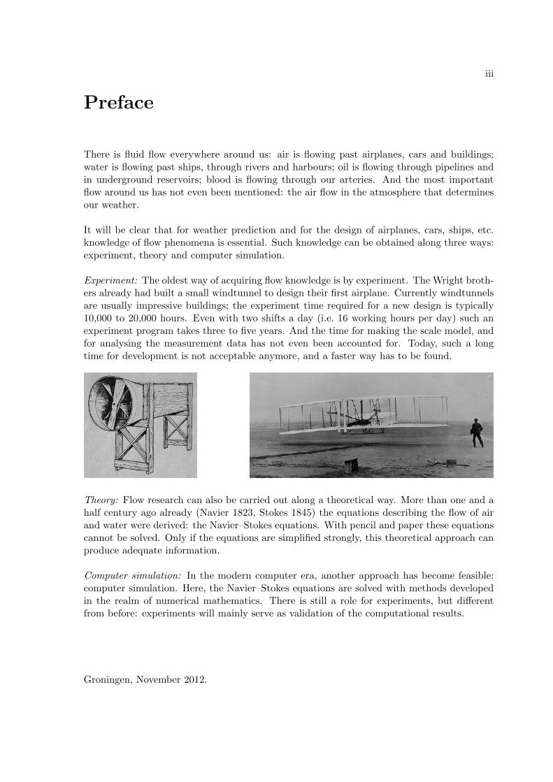
Experiment: The oldest way of acquiring flow knowledge is by experiment. The Wright broth-ers already had built a small windtunnel to design their first airplane. Currently windtunnelsare usually impressive buildings; the experiment time required for a new design is typically10,000 to 20,000 hours. Even with two shifts a day (i.e. 16 working hours per day) such anexperiment program takes three to five years. And the time for making the scale model, andfor analysing the measurement data has not even been accounted for. Today, such a longtime for development is not acceptable anymore, and a faster way has to be found.
Theory: Flow research can also be carried out along a theoretical way. More than one and ahalf century ago already (Navier 1823, Stokes 1845) the equations describing the flow of airand water were derived: the Navier–Stokes equations. With pencil and paper these equationscannot be solved. Only if the equations are simplified strongly, this theoretical approach canproduce adequate information.
Computer simulation: In the modern computer era, another approach has become feasible:computer simulation. Here, the Navier–Stokes equations are solved with methods developedin the realm of numerical mathematics. There is still a role for experiments, but differentfrom before: experiments will mainly serve as validation of the computational results.
Groningen, November 2012.

iv

Contents
1 The convection-diffusion equation 1
1.1 Analytical formulation . . . . . . . . . . . . . . . . . . . . . . . . . . . . . . . 1
1.2 Central versus upwind discretization . . . . . . . . . . . . . . . . . . . . . . . 2
1.2.1 Analytical problem . . . . . . . . . . . . . . . . . . . . . . . . . . . . . 2
1.2.2 Discretization . . . . . . . . . . . . . . . . . . . . . . . . . . . . . . . . 3
1.2.3 Solution with central discretization . . . . . . . . . . . . . . . . . . . . 4
1.2.4 Solution with upwind discretization . . . . . . . . . . . . . . . . . . . 6
1.3 Artificial diffusion . . . . . . . . . . . . . . . . . . . . . . . . . . . . . . . . . 7
1.3.1 Second-order diffusion . . . . . . . . . . . . . . . . . . . . . . . . . . . 7
1.3.2 Higher-order additives . . . . . . . . . . . . . . . . . . . . . . . . . . . 9
1.4 Preliminary trade-off . . . . . . . . . . . . . . . . . . . . . . . . . . . . . . . . 10
1.5 Non-uniform grids . . . . . . . . . . . . . . . . . . . . . . . . . . . . . . . . . 12
1.5.1 Discretization . . . . . . . . . . . . . . . . . . . . . . . . . . . . . . . . 12
1.5.2 Numerical benchmark . . . . . . . . . . . . . . . . . . . . . . . . . . . 14
1.5.3 Discussion: steady . . . . . . . . . . . . . . . . . . . . . . . . . . . . . 15
1.5.4 Discussion: unsteady . . . . . . . . . . . . . . . . . . . . . . . . . . . . 17
1.5.5 Iterative solution . . . . . . . . . . . . . . . . . . . . . . . . . . . . . . 18
1.6 Finite-volume discretization . . . . . . . . . . . . . . . . . . . . . . . . . . . . 19
1.6.1 One space dimension . . . . . . . . . . . . . . . . . . . . . . . . . . . . 19
1.6.2 More space dimensions . . . . . . . . . . . . . . . . . . . . . . . . . . . 21
1.7 Higher-order space discretization . . . . . . . . . . . . . . . . . . . . . . . . . 23
1.8 Time integration . . . . . . . . . . . . . . . . . . . . . . . . . . . . . . . . . . 27
1.8.1 Stability analysis . . . . . . . . . . . . . . . . . . . . . . . . . . . . . . 27
1.8.2 Practical example . . . . . . . . . . . . . . . . . . . . . . . . . . . . . 29
1.9 Burgers’ equation – discontinuous solutions . . . . . . . . . . . . . . . . . . . 31
1.10 ‘Convective’ conclusions . . . . . . . . . . . . . . . . . . . . . . . . . . . . . . 35
1.11 Appendix: Dirichlet–Neumann stability analysis . . . . . . . . . . . . . . . . 35
1.12 References . . . . . . . . . . . . . . . . . . . . . . . . . . . . . . . . . . . . . . 37
2 Incompressible Navier–Stokes equations 39
2.1 The equations for fluid flow . . . . . . . . . . . . . . . . . . . . . . . . . . . . 39
2.2 Choice of the computational grid . . . . . . . . . . . . . . . . . . . . . . . . . 41
2.3 Discretization - explicit . . . . . . . . . . . . . . . . . . . . . . . . . . . . . . 44
2.4 The Poisson equation for the pressure . . . . . . . . . . . . . . . . . . . . . . 47
2.4.1 Boundary conditions . . . . . . . . . . . . . . . . . . . . . . . . . . . . 47
2.4.2 Treatment of div u(n) . . . . . . . . . . . . . . . . . . . . . . . . . . . 50
v
vi CONTENTS
2.4.3 Pressure iteration . . . . . . . . . . . . . . . . . . . . . . . . . . . . . . 512.5 The steady Navier–Stokes equations . . . . . . . . . . . . . . . . . . . . . . . 52
2.5.1 Discrete formulation . . . . . . . . . . . . . . . . . . . . . . . . . . . . 522.5.2 Artificial compressibility . . . . . . . . . . . . . . . . . . . . . . . . . . 532.5.3 SIMPLE . . . . . . . . . . . . . . . . . . . . . . . . . . . . . . . . . . . 53
2.6 Discretization - implicit . . . . . . . . . . . . . . . . . . . . . . . . . . . . . . 542.6.1 Linearization . . . . . . . . . . . . . . . . . . . . . . . . . . . . . . . . 552.6.2 Pressure correction . . . . . . . . . . . . . . . . . . . . . . . . . . . . . 56
2.7 In- and outflow conditions . . . . . . . . . . . . . . . . . . . . . . . . . . . . . 582.8 References . . . . . . . . . . . . . . . . . . . . . . . . . . . . . . . . . . . . . . 59
3 Direct numerical simulation of turbulence 613.1 Computational effort . . . . . . . . . . . . . . . . . . . . . . . . . . . . . . . . 613.2 Navier–Stokes: higher-order space discretization . . . . . . . . . . . . . . . . . 643.3 Refined time integration . . . . . . . . . . . . . . . . . . . . . . . . . . . . . . 663.4 Examples of turbulent-flow simulation . . . . . . . . . . . . . . . . . . . . . . 68
3.4.1 Flow past a square cylinder at Re = 22,000 . . . . . . . . . . . . . . . 683.4.2 Surface mounted cubes . . . . . . . . . . . . . . . . . . . . . . . . . . . 713.4.3 Channel flow . . . . . . . . . . . . . . . . . . . . . . . . . . . . . . . . 74
3.5 References . . . . . . . . . . . . . . . . . . . . . . . . . . . . . . . . . . . . . . 76
A Discretization, integration and iteration 79A.1 Discretization in space . . . . . . . . . . . . . . . . . . . . . . . . . . . . . . . 79
A.1.1 Finite-difference methods . . . . . . . . . . . . . . . . . . . . . . . . . 80A.1.2 Finite-volume methods . . . . . . . . . . . . . . . . . . . . . . . . . . . 80A.1.3 Properties of difference operators . . . . . . . . . . . . . . . . . . . . . 81A.1.4 Discretization error . . . . . . . . . . . . . . . . . . . . . . . . . . . . . 83
A.2 Elementary iterative solution methods . . . . . . . . . . . . . . . . . . . . . . 84A.2.1 Jacobi and JOR . . . . . . . . . . . . . . . . . . . . . . . . . . . . . . 84A.2.2 Gauss-Seidel and SOR . . . . . . . . . . . . . . . . . . . . . . . . . . . 86A.2.3 Some definitions and theorems on eigenvalues . . . . . . . . . . . . . . 88
A.3 Integration in time . . . . . . . . . . . . . . . . . . . . . . . . . . . . . . . . . 89A.3.1 Stability . . . . . . . . . . . . . . . . . . . . . . . . . . . . . . . . . . . 90A.3.2 Matrix analysis . . . . . . . . . . . . . . . . . . . . . . . . . . . . . . . 91A.3.3 Positive time-integration schemes . . . . . . . . . . . . . . . . . . . . . 92A.3.4 Fourier analysis . . . . . . . . . . . . . . . . . . . . . . . . . . . . . . . 93A.3.5 The modified equation . . . . . . . . . . . . . . . . . . . . . . . . . . . 98
A.4 References . . . . . . . . . . . . . . . . . . . . . . . . . . . . . . . . . . . . . . 99
B Computer exercises 101B.1 Exercise 1 – Artificial diffusion . . . . . . . . . . . . . . . . . . . . . . . . . . 101B.2 Exercise 2 – Various discretization methods . . . . . . . . . . . . . . . . . . . 102B.3 Exercise 3 – The JOR and SOR method . . . . . . . . . . . . . . . . . . . . . 104B.4 Exercise 4 – Time integration . . . . . . . . . . . . . . . . . . . . . . . . . . . 107B.5 Exercise 5 – Navier–Stokes solver . . . . . . . . . . . . . . . . . . . . . . . . . 109

Chapter 1
The convection-diffusion equation
1.1 Analytical formulation
The discussion of numerical solution methods for the equations of fluid flow starts with a‘simple’ situation: the transport of a solute in a flowing medium. Two transport mechanismscan be distinguished: convection and diffusion.
convection = transport due to the motion of the medium;diffusion = transport due to differences in concentration.
The concentration of solute is denoted by φ(x, t), where x represents space and t time. Theflowing medium is assumed to be incompressible, with a velocity u(x, t).
The equation describing the concentration as a function of space and time can be derivedfrom a conservation law. Hereto, consider an arbitrary volume Ω with boundary Γ andoutward pointing normal n. A decrease of the amount of solute inside the volume Ω is dueto outward transport of solute through the boundary Γ. The convective transport per unitof time is given by ∫
Γφu · ndΓ;
the diffusive transport by ∫Γ−k gradφ · ndΓ,
where the diffusion has been taken proportional to the gradient of the concentration (diffusioncoefficient k ≥ 0).
Conservation of mass in Ω yields∫Ω
∂φ
∂tdΩ = −
∫Γ(φu− k gradφ) · ndΓ = (Gauss)
= −∫
Ωdiv (φu− k gradφ) dΩ.
As this holds for any arbitrary volume Ω, it follows that
∂φ
∂t+ div (φu− k gradφ) = 0. (1.1)
1

2 CHAPTER 1. THE CONVECTION-DIFFUSION EQUATION
This is called the divergence form of the equation. When divu = 0 (incompressibility condi-tion) the convection-diffusion equation can be rewritten in its more common form
∂φ
∂t+ u · gradφ = div (k gradφ).
Remark 1 Equation (1.1) also describes heat transport in a flowing medium with φ thetemperature. The diffusion corresponds with heat conduction.
Remark 2 The above mass balance can also be considered in discrete form; the finite-volumemethod results. More on this method in Section 1.6 and Appendix A.1.2.
1.2 Central versus upwind discretization
1.2.1 Analytical problem
We start with the steady convection-diffusion equation in one space dimension, with a velocityfield u and a diffusion coefficient k that are taken constant
Lφ ≡ u dφ
dx− k d2φ
dx2= 0 (0 < x < L) φ(0) = T0, φ(L) = TL. (1.2)
The solution to this equation is given by
φ(x) = T0 + (TL − T0)1− eux/k
1− euL/k≡ T0 + (TL − T0)
1− ePe(x/L)
1− ePe, (1.3)
in which
Pe ≡ uL
kis the Peclet number.
For moderate values of Pe the solution φ(x) varies smoothly over the whole domain. WhenPe is large, the solution possesses a boundary-layer character in which φ(x) ≈ T0, except ina thin layer of thickness k/u(= L/Pe) near the outflow boundary x = L where the solutionadapts itself to the outflow condition φ(L) = TL.
0
0.5
1
0 0.2 0.4 0.6 0.8 1x
φ
Pe = 1
Pe = 10
Pe = 50
Exact solution of convection-diffusion equation for variousvalues of the Peclet numberPe.

1.2. CENTRAL VERSUS UPWIND DISCRETIZATION 3
Remark The fastest way to ‘prove’ that the boundary layer thickness is proportional tok/u uses dimensional analysis. First recognise that u has dimension m/sec, whereas k hasdimension m2/sec. Then conclude that k/u is the only combination that can be made withthe physical parameters that has a dimension of length.
1.2.2 Discretization
The convection-diffusion equation (1.2) will be discretized on a grid with grid points xi =ih, h = L/I, i = 0, · · · , I. Various ways exist of discretizing partial differential equations;in these lecture notes we will follow either a finite-difference or a finite-volume approach(see Appendix A.1). Let us start simple with a finite-difference approximation of the partialderivatives occurring in (1.2).
With second-order central discretization we have
dφ
dx=φi+1 − φi−1
2h+O(h2);
d2φ
dx2 =φi+1 − 2φi + φi−1
h2 +O(h2). (1.4)
For the discretized operator Lch this means
(Lchφh)i ≡(u
2h− k
h2
)φi+1 +
2k
h2φi +
(− u
2h− k
h2
)φi−1 = 0. (1.5)
-2
-1
0
1
0 0.2 0.4 0.6 0.8 1x
φ
Pe = 500
Let us first demonstrate the centrally dis-cretized solution for a situation where Pe =500. The grid in this example consists of 10grid points. One observes that the discretesolution shows enthusiastic wiggles. To under-stand this we need the notion of a monotoneoperator, as discussed in Appendix A.1.
Remark In this example, the wiggles are trig-gered by the Dirichlet condition at x = 1 witha value that does not ‘match’ the value of φin the interior. Here, we do this on purpose toshow their occurrence, their origin and somestrategies to prevent them. In Section 2.7 wewill show how these wiggles can be suppressed by choosing a more appropriate boundarycondition. However, it is good to realize that wiggles can also be induced by other reasons,e.g. near shock waves.
If the requirements for being a monotone operator are compared with the properties ofthe discrete scheme given by (1.5), the following can be concluded:
Theorem 1.2.1 The operator Lch is positive if and only if the mesh-Peclet number P satisfies
P ≡ |u|hk≤ 2. (1.6)
It is monotone, i.e. a maximum principle holds, if P < 2.

4 CHAPTER 1. THE CONVECTION-DIFFUSION EQUATION
Proof For a definition of a positive operator we first refer to Appendix A.1. Further it is assumed
that u > 0. In that case the coefficient of φi−1, given in (1.5), clearly is always negative, and only
the coefficient of φi+1 might give troubles. The latter coefficient is given by u/2h − k/h2, which is
non-positive precisely under the condition (1.6). For a maximum principle to hold, the coefficients
have to be strictly negative (Th. A.1.2). 2
The above condition stresses that when using central discretization the mesh width h hasto be sufficiently small in order to obtain a positive operator. In the latter case the solutionwill be wiggle-free. A physicists reaction would be: “If you want to compute the boundarylayer, then the least thing to do is to fit your grid size to the boundary-layer thickness, i.e.choose h = k/u.” This insight is helpful, as for this choice of the grid size the mesh Pecletnumber becomes equal to 1 (which is smaller than 2!).
A small grid size leads to a large number of grid points and hence an expensive calcu-lation. And maybe you are not really interested in the details within the boundary layer,i.e. convection is considered to be much more important than diffusion. In that case ourphysicist friend has an advice concerning the discretization of the convective term: “If thewind is blowing from a particular direction, then you only have to look in that direction tosee what is coming towards you.” With this physical insight, in fact he suggests to consideran alternative, one-sided discretization of the first order derivative
dφ
dx=
φi − φi−1
h+O(h) (u ≥ 0),
φi+1 − φih
+O(h) (u < 0).
(1.7)
(1.7) is called an ‘upwind’ discretization, be-cause it is taken against the direction of theflow velocity u. This discretization is first-order accurate – in contrast with the second-order accuracy of (1.4) – but it always leadsto a (monotone) positive operator irrespec-tive of the mesh width h, as can be easilydeduced (see Exercise 1.2.1). The discreteresults in the same case as above indeed donot possess wiggles! But are they accurate?We will come back to this question later.
0
0.5
1
0 0.2 0.4 0.6 0.8 1x
φ Pe = 500 upwind
Exercise 1.2.1 Prove that, for k > 0, upwind discretization always leads to a positive and monotoneoperator.
1.2.3 Solution with central discretization
The central discretization (1.5) can be rewritten as
P
2(φi+1 − φi−1)− (φi+1 − 2φi + φi−1) = 0 (i = 1, . . . , I − 1), (1.8)

1.2. CENTRAL VERSUS UPWIND DISCRETIZATION 5
in which the mesh-Peclet number P = uh/k dominantly features. In fact, when P becomeslarge and φ remains bounded, this equation simplifies to
φi+1 − φi−1 ≈ 0. (1.9)
In other words, grid points two meshes apart are closely connected to each other, but theyare independent of their direct neighbours. This phenomenon is called odd-even decoupling.
The difference equation (1.8) can be solved analytically by means of the next lemma.
Lemma 1.2.2 When a 6= b, the solution of the difference equation aφi+1−(a+b)φi+b φi−1 =0 (i = 1, . . . , I − 1), with boundary conditions φ0 = T0 and φI = TL, is given by
φi = T0 + (TL − T0)1− ri
1− rIwhere r =
b
a. (1.10)
Note that the solution will oscillate when r < 0, i.e. when a and b have a different sign.Compare this with the wiggles that can appear for non-positive operators (see Appendix A.1).
Proof Find fundamental solutions of the form ri. These satisfy the characteristic equation ar2− (a+
b)r+b = 0, which leads to r1 = 1 and r2 = b/a. Now, the general solution is given by φi = c1ri1 +c2r
i2.
The boundary conditions at i = 0 and i = I fix the coefficients c1 and c2, after which (1.10) follows.
2
Application of the above lemma gives the exact solution of (1.8)
φi = T0 + (TL − T0)1−
(1+P/21−P/2
)i1−
(1+P/21−P/2
)I , (i = 0, . . . , I).
We will consider this solution for large values of P . Introduce ε ≡ 2/P 1 and apply seriesexpansion in ε
φi = T0 + (TL − T0)1− (−1)i(1 + 2iε)
1− (−1)I(1 + 2Iε)+O(ε2). (1.11)
Distinguish the cases I is even/odd and i is even/odd.
• I odd:When I is odd (1.11) becomes
φi ≈ T0 + (TL − T0)1− (−1)i − 2(−1)iiε
2(1 + Iε),
hence
i even: φi ≈ T0 − (TL − T0) iε; i odd: φi ≈ TL − (TL − T0)(I − i)ε.
The solution in even grid points fits to the left-hand-side boundary condition, whereasthe odd points fit to the right-hand-side condition. This is a concrete example of theodd/even decoupling announced above.

6 CHAPTER 1. THE CONVECTION-DIFFUSION EQUATION
• I even:When I is even we have
φi ≈ T0 + (TL − T0)1− (−1)i(1 + 2iε)
−2Iε,
hence
i even: φi ≈ T0 + (TL − T0)i
I; i odd: φi ≈ T0 + (TL − T0)
(−1
Iε− i
I
).
The solution in the even grid points fits to both boundary conditions. Odd grid pointslook awful: the solution there approaches infinity when ε→ 0. Note that φi is no longerbounded, hence (1.9) does not describe the behaviour.
-2
-1
0
1
0 0.2 0.4 0.6 0.8 1x
φ
Pe = 500
-2
-1
0
1
0 0.2 0.4 0.6 0.8 1x
φ
Pe = 500
Central discretization for Pe = 500: I odd (left) and I even (right).
1.2.4 Solution with upwind discretization
When an upwind discretization (1.7) is applied, the discrete equation becomes (assumingu > 0)
P (φi − φi−1)− (φi+1 − 2φi + φi−1) = 0, φ0 = T0, φI = TL.
The solution again follows from (1.10)
φi = T0 + (TL − T0)1− (1 + P )i
1− (1 + P )I.
For P large we have
φi ≈ T0 + (TL − T0)P i−I ,
which for i < I is approximately equal to T0, whereas φI = TL. The solution does not possesswiggles and looks more friendly than the central solution. But the boundary layer is toothick! The two figures below show the upwind solution and the exact solution for a situation

1.3. ARTIFICIAL DIFFUSION 7
with I = 10, k = 0.002, T0 = 0 and TL = 1.
0
0.5
1
0 0.2 0.4 0.6 0.8 1x
φ Pe = 500 upwind
0
0.5
1
0 0.2 0.4 0.6 0.8 1x
φ Pe = 500 exact
Upwind discretization Exact solution
1.3 Artificial diffusion
1.3.1 Second-order diffusion
If we compare the (second-order) central discretization with the (first-order) upwind dis-cretization through
uφi − φi−1
h≡ u φi+1 − φi−1
2h− uh
2
φi+1 − 2φi + φi−1
h2,
it is observed that upwind discretization of (1.2) yields the same discrete equation as centraldiscretization of
udφ
dx−(k +
uh
2
)d2φ
dx2= 0. (1.12)
When comparing the centrally discretized solution of (1.2) with the upwind discretized solu-tion of (1.2), the formulation (1.12) can be used as an intermediate step.
upwinddiscretization
of (1.2)≡
centraldiscretization
of (1.12)←→
centraldiscretization
of (1.2)
It is observed that (1.12) in comparison with (1.2) contains an additional term in whichthe diffusion coefficient is increased with ka = uh/2. This increase is called artificial diffu-sion. When the artificial diffusion dominates the real diffusion, and when one is interested inthe effects of diffusion, then the usefulness of the upwind discretized solution decreases. Butbe aware! We have silently assumed that the other discretization errors are small and thatthey do not play a role in the above. If this is not the case then the judgement on upwinddiscretization can be more positive. Also when diffusion is not relevant for the physics thereis little harm in increasing the diffusion, making upwind discretization an acceptable choice.

8 CHAPTER 1. THE CONVECTION-DIFFUSION EQUATION
The advantage of upwind discretization is that a (monotone) positive operator is created,which is easily treated iteratively (see Appendix A.2). Also other choices for the artificialviscosity ka lead to a positive operator. To investigate this, let us discretize the equation
udφ
dx− (k + ka)
d2φ
dx2= 0 (1.13)
for arbitrary ka using central discretization. We obtain
(Lahφh)i ≡uh
2(φi+1 − φi−1)− (k + ka) (φi+1 − 2φi + φi−1) = 0.
With reference to Theorem 1.2.1, the operator Lah is a positive operator if and only if
k + ka ≥|u|h
2⇔ ka ≥
|u|h2− k.
The upwind discretization with ka = |u|h/2 satisfies this criterion. In the literature also otherchoices can be found. The figure below shows the quantity ka/k, for a number of methods,as a function of P = |u|h/k.
-
6
ka/k
P
UD
ASSp
UD = upwind discretization
Sp = Spalding (1972):
ka = max (0, |u|h2 − k)
AS = Allen & Southwell (1955)
0 2 4 60
1
2
3
A special choice for ka has been described for the first time by Allen & Southwell (1955),and reinvented many times. Gresho & Lee (1981) call it the ‘smart upwind’ method. Othernames are the ‘locally exact’ method, and the ‘exponential scheme’. This special choice of kacan be found by comparing (1.3) and (1.10). One notes that for r = ePe/I = eP the discretesolution (1.10) and the analytic solution (1.3) in the grid points are equal. This situationarises when (1.13) is centrally discretized with an artificial diffusion coefficient (assume u > 0)
ka =uh
2coth
P
2− k = k
(P
2coth
P
2− 1
). (1.14)
Proof After central discretization of (1.13), an equation as in Lemma 1.2.2 is obtained with
a ≡ u
2h− k + ka
h2and b ≡ − u
2h− k + ka
h2.
Requiring that z ≡ b/a = eP , we can work backward to ‘reconstruct’ ka:
− u
2h− k + ka
h2= eP
(u
2h− k + ka
h2
)⇒ k+ka =
uh
2
(eP + 1
eP − 1
)=uh
2
(eP/2 + e−P/2
eP/2 − e−P/2
).
2

1.3. ARTIFICIAL DIFFUSION 9
For small P the expression between parentheses in (1.14) approaches zero, hence in thiscase no artificial diffusion is added. The discrete solution will now approach the solution of thecentrally discretized problem. For large P , ka behaves like ka ≈ 1
2uh− k. The solution thenresembles the upwind discretized solution. Yet, for the above one-dimensional convection-diffusion equation with constant coefficients the exact solution is obtained. In more than onedimension, nothing similar has been found yet.
Artificial diffusion is often applied in situations with P > 2, i.e. 12h > k/u = the boundary-
layer thickness, to obtain a system of discrete equations which is easier tractable numerically.When the solution is smooth - the amount of diffusion is not important then - this does notmatter very much. However, when the solution should possess a boundary-layer characterthe mesh width simply is too large to resolve details in the boundary layer. No choice of kacan repair this situation, not even (1.14) which gives the exact solution! A smooth solution iscreated, however its boundary layer is too thick1. This can be seen only by comparing withthe exact solution. The left-hand-side figure on page 7 looks nice, but comparison with theexact solution shows that the boundary layer is not computed correctly. In such a situationthe centrally discretized solution gives a warning by showing violent wiggles (see the figures onpage 6); compare Gresho & Lee (1981). When the details in the boundary layer are relevant,the only remedy is to refine the mesh width such that at least a few grid points are locatedinside the boundary layer. Then automatically P ≤ 2 inside the boundary layer (check this!).Outside the boundary layer P > 2, but that need not be critical (see Section 1.5).
1.3.2 Higher-order additives
The wiggle-dependence of central discretization of a first-order derivative also can be dimin-ished by adding a term of the form h2 d3φ/dx3 (for u > 0)2
dφ
dx=φi+1 − φi−1
2h− λ φi+1 − 3φi + 3φi−1 − φi−2
h+ τh, (1.15)
with
τh = h2
(λ− 1
6
)φxxx +O(h3).
Here we have a family of upwind-biased λ-schemes3, which all are second-order accurate; forλ = 1/6 we even have a third-order discretization. Special cases are further λ = 0 (centraldiscretization), λ = 1/2 (second-order upwind: the B3-scheme in which φi+1 drops out) andλ = 1/8 (the QUICK method).
Why λ = 1/8 is a special value, can be seen as follows. Consider in the figure below thepoints R and L which lie halfway [i, i + 1], and [i − 1, i], respectively. We approximate the
1With upwind diffusion ka ≡ uh/2, the thickness of the (artificial) boundary layer becomes ka/u = h/2,i.e. it can be resolved by the grid.
2An upwind-biased second-order discretization of a third-order derivative is given by
d3φ
dx3=φi+1 − 3φi + 3φi−1 − φi−2
h3.
3Above upwind-biased schemes are also used, in disguised form, in compressible flow, where they are calledκ-schemes; see e.g. Hirsch (1990) or Wesseling (2001). They are equivalent when κ = 1− 4λ.

10 CHAPTER 1. THE CONVECTION-DIFFUSION EQUATION
derivative in i in a finite-volume fashion through
i− 2 i− 1 i i+ 1L R
dφ
dx=φR − φL
h.
The values φR and φL are determined via quadraticinterpolation on the intervals [i−1, i+1], and [i−2, i]respectively (assuming u > 0). In this way
φR =φi+1 + φi
2− φi+1 − 2φi + φi−1
8,
with a similar formula for φL. QUICK stands for Quadratic Upstream Interpolation for Con-vective Kinematics (Leonard 1979).
After having added a second-order derivative and a third-order derivative to ‘smooth’central discretization, it sounds logical that a fourth-order derivative (multiplied by h3) alsomight be useful. Indeed this is the case. Jameson et al. (1981) have introduced this approachfor solving the inviscid Euler equations, but we will not go into further detail here. Anotherway of getting rid of the wiggles is to apply monotone discretization methods, where keywordslike ‘limiters’ and ‘TVD (total variation diminishing)’ are issues; see e.g. Chapters 20 and 21of Hirsch (1990) or Chapter 9 of Wesseling (2001).
Exercise 1.3.1 Prove that λ ≥ max( 12−
k|u|h , 0) is a sufficient condition for the upwind-biased methods
from (1.15) to be wiggle-free. Show that the QUICK method is wiggle-free for P ≤ 8/3. Hint: Tryfundamental solutions of the form ri, and monitor the sign of r.
1.4 Preliminary trade-off
The trade-off between the methods presented above (and the methods still to be presented)is a delicate matter. An important role is played by the ratio between the mesh size and thelength scales of the solution.
To give a first impression we have compared a number of methods:
i) the first-order upwind method (1.7);ii) the second-order upwind method (1.15) with λ = 1/2;iii) the QUICK method (1.15) with λ = 1/8;iv) the second-order central method (1.4);v) the fourth-order central method (see Section 1.7). s
ssssccc
c ccc ccc c c
The difference stencils of methods ii), iii) and v) are too large near the boundaries. There-fore, where necessary in the first and last grid points a central discretization has been applied.Except for the fourth-order method, the diffusive term has been discretized with the second-order discretization as used in (1.4). Thus, it makes not much sense to include the third-orderλ-scheme with λ = 1/6 in this comparison, as the second-order error from diffusion will dom-inate for small grid sizes; anyway its results do not differ dramatically from those for λ = 1/8.
1.4. PRELIMINARY TRADE-OFF 11
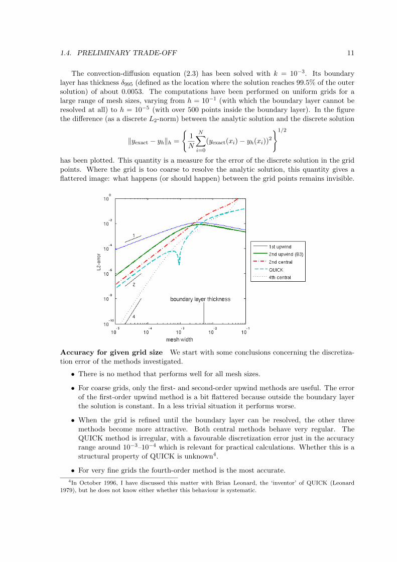
The convection-diffusion equation (2.3) has been solved with k = 10−3. Its boundarylayer has thickness δ995 (defined as the location where the solution reaches 99.5% of the outersolution) of about 0.0053. The computations have been performed on uniform grids for alarge range of mesh sizes, varying from h = 10−1 (with which the boundary layer cannot beresolved at all) to h = 10−5 (with over 500 points inside the boundary layer). In the figurethe difference (as a discrete L2-norm) between the analytic solution and the discrete solution
‖yexact − yh‖h =
1
N
N∑i=0
(yexact(xi)− yh(xi))2
1/2
has been plotted. This quantity is a measure for the error of the discrete solution in the gridpoints. Where the grid is too coarse to resolve the analytic solution, this quantity gives aflattered image: what happens (or should happen) between the grid points remains invisible.
Accuracy for given grid size We start with some conclusions concerning the discretiza-tion error of the methods investigated.
• There is no method that performs well for all mesh sizes.
• For coarse grids, only the first- and second-order upwind methods are useful. The errorof the first-order upwind method is a bit flattered because outside the boundary layerthe solution is constant. In a less trivial situation it performs worse.
• When the grid is refined until the boundary layer can be resolved, the other threemethods become more attractive. Both central methods behave very regular. TheQUICK method is irregular, with a favourable discretization error just in the accuracyrange around 10−3–10−4 which is relevant for practical calculations. Whether this is astructural property of QUICK is unknown4.
• For very fine grids the fourth-order method is the most accurate.
4In October 1996, I have discussed this matter with Brian Leonard, the ‘inventor’ of QUICK (Leonard1979), but he does not know either whether this behaviour is systematic.

12 CHAPTER 1. THE CONVECTION-DIFFUSION EQUATION
Computational effort Next, the effort to solve the discrete system of equations should beconsidered. It will be clear that a larger difference stencil will lead to a less sparse matrix,making direct solution more expensive. Yet, for small (2D) problems direct methods will bethe fastest. When the system is solved iteratively, the upwind method is very easy to handle.The other methods require a more sophisticated iterative treatment, which usually will bemore expensive. However, when this iteration process can be combined with other iterativeprocesses, e.g. treating non-linearity, the computational pain will be relieved. Over the years,many useful methods have been presented in the literature (for the developments at RUG seee.g. Wubs and Thies 2011).
Maintainability A final aspect to be taken into account is the simplicity of the method andherewith the simplicity of the computer code. Methods with a larger stencil require specialmeasures near the boundaries, introducing many exceptional cases, and increasing the chancefor errors: the code becomes less readable and less maintainable.
Trade-off
• For engineering accuracy (say 10−3) I would prefer a second-order central discretization:a small stencil, and easy to implement. Of course, the grid size has to be adapted to thebehaviour of the solution: too coarse meshes can lead to large oscillations, as explainedabove. The QUICK method, with its larger stencil, is still a mystery to me.
• For coarse-grid calculations only the upwind methods qualify. First-order upwind iseasily handled, but its results are accordingly. Second-order upwind is remarkablybetter, but it has the disadvantage of a larger stencil. It is the only method withreasonable performance for a large range of mesh sizes.
• Only when one is interested in four or more figures accuracy the fourth-order methodsare of interest. One should take into account that the equations to be solved oftenwill be an approximation of reality containing modelling errors. There is no sense inreducing the discretization error too far below this modelling error.
In the next sections we will discuss more advanced discretization methods with which theirprice/performance ratio can be improved.
1.5 Non-uniform grids
Thus far grids have been used in which, per coordinate direction, the mesh size is constant.In practice often grids with varying mesh size are used. Their purpose is to describe thesolution, at prescribed accuracy, with as little grid points as possible. In this way the discretesystems to be solved become smaller, and in general – but not always (cf. Exercise 1.5.1)! –can be solved cheaper.
1.5.1 Discretization
We start with a study of the local discretization error on a non-equidistant grid. Hereto we usea one-dimensional example in which a first-order and a second-order derivative are discretized.

1.5. NON-UNIFORM GRIDS 13
Consider the following triple of grid points, with function values φ−, φ0 and φ+, and atmutual distances h− and h+
x− x0 x+
h− h+φ− φ0 φ+u u u
In the middle grid point the derivatives φx and φxx are approximated with finite-differenceformulas in which only φ−, φ0 and φ+ appear. We start with the Taylor series for φ+ andφ−:
φ+ = φ0 + h+φx + 12h
2+φxx + 1
6h3+φxxx + · · · , (1.16)
φ− = φ0 − h−φx + 12h
2−φxx − 1
6h3−φxxx + · · · . (1.17)
When we simply subtract (1.16) and (1.17) we obtain (Method A)
φx =φ+ − φ−h+ + h−
− 12(h+ − h−)φxx − 1
6
h3+ + h3
−h+ + h−
φxxx + · · ·
=h+
h+ + h−φ+ − φ0h+
+h−
h+ + h−φ0 − φ−h−
+ · · · .(1.18)
On uniform grids the term (h+ − h−)φxx vanishes; this term is related to the stretching ofthe grid (see below). Geometrically this estimate for the derivative in the i-th grid pointis generated by means of a linear interpolation of φ between the adjacent grid points (for afinite-volume interpretation see Section 1.6).
tt
tMethod A
Method B
x− x0 x+
- -h− h+
φ−
φ0
φ+
((((((((
((((((
hhhhhhhhhhhhhh
By combining (1.16) and (1.17) in a different way, the term with φxx can be eliminatedbeforehand. Take h2
− × (1.16)− h2+ × (1.17), then one obtains (Method B)
φx =h2− φ+ +
(h2
+ − h2−)φ0 − h2
+ φ−h+h−(h+ + h−)
− 16h+h−φxxx + · · ·
=h−
h+ + h−φ+ − φ0h+
+h+
h+ + h−φ0 − φ−h−
+ · · · .(1.19)
First observe that the weights of the forward and backward derivatives have been interchangedin comparison with (1.18). Further, the local discretization error in (1.19) looks better thanthe one in (1.18). Not only a term with φxx is missing, but also the coefficient of φxxx isless or equal the corresponding coefficient in (1.18). Again a geometric interpretation can begiven. Draw a parabola through the three points φ−, φ0 and φ+ (Lagrange interpolation),then the tangent to this parabola in φ0 gives the estimate (1.19). Note that, because of theseTaylor-series considerations, (1.19) is the ‘standard’ central discretization for a first-orderderivative. However, in the next section we will see that it does possess serious drawbacks.

14 CHAPTER 1. THE CONVECTION-DIFFUSION EQUATION
For the approximation of φxx, only one feasible option is available: combine h−× (1.16) +h+ × (1.17)
φxx =h− φ+ − (h+ + h−)φ0 + h+ φ−
12h+h−(h+ + h−)
− 13(h+ − h−)φxxx + · · · . (1.20)
Again the difference h+ − h− appears. In the literature it is often called a first-order term,but it can equally well be called a second-order term: this depends on the way in which themesh width approaches zero. When h+ and h− approach zero with h+/h− = constant 6= 1,it is a first-order term. It is a second-order term when the grid is obtained through a trans-formation, x = f(ξ), in which the ξ-interval is divided uniform with mesh width ∆. From aTaylor series around ξ0 (corresponding with the central point) we get
h+ ≡ x+ − x0 = ∆f ′(ξ0) + 12∆2f ′′(ξ0) + · · · ,
h− ≡ x0 − x− = ∆f ′(ξ0)− 12∆2f ′′(ξ0) + · · · ,
hence
h+ − h− = ∆2f ′′(ξ0) + · · · andh+
h−= 1 + ∆
f ′′
f ′(ξ0) + · · · .
It will be clear that f ′′(ξ) controls the amount of stretching of the grid.
1.5.2 Numerical benchmark
0
0.5
1
0 0.2 0.4 0.6 0.8 1x
φ
Method B
0
0.5
1
0 0.2 0.4 0.6 0.8 1x
φ
Method A
Discretization according to Method B(1.19) yields the above result.
Discretization by Method A (1.18), whichlooks less promising then (1.19) whenmeasuring the local truncation error, pro-duces much better results.
The difference between both discretization methods A and B will be demonstrated witha few examples. Consider the model problem (1.2) on the interval 0 ≤ x ≤ 1, with u = 1 andk = 0.002 and boundary conditions φ(0) = 0 and φ(1) = 1. The exact solution is shown onpage 7. In the examples we use a grid given by
xi = 0, 0.2− k, 0.4− 2k, 0.6− 3k, 0.8− 4k, 1− 5k, 1− 4k, 1− 3k, 1− 2k, 1− k, 1, (1.21)
hence for k = 0.002 we have five grid cells of size about 0.2 and five grid cells of size 0.002.

1.5. NON-UNIFORM GRIDS 15
For comparison we show the discretesolution from upwind discretization.
0
0.5
1
0 0.2 0.4 0.6 0.8 1x
φ
x
φ
x
φ
upwind
1.5.3 Discussion: steady
The above example gives an impression of the systematic behaviour of both methods; moreexamples can be found in Veldman et al. (1991, 1993) and Verstappen and Veldman (1997,1998, 2003). We will now give a fundamental explanation of the observed behaviour.
To get a feeling of the relation between the local discretization (= truncation) error (as in(1.18) and (1.19)) and the global discretization error we have to consider (see Appendix A.1)
φexact − φh = L−1h τ h. (1.22)
This relation shows that the global error is determined by multiplying the local error withthe inverse of the coefficient matrix. When the diagonal of Lh is weakened, roughly spoken,some eigenvalues may move towards zero herewith ‘increasing’ L−1
h . In the examples shown,for Method B this increase of L−1
h apparently overrules the decrease of τ h. Let us analysethis in more detail.
Consider first the coefficient matrix LA of Method A, defined from (1.18) and (1.20),which will be scaled by a diagonal matrix H incorporating the local grid size
MA = HLA where H = diag
h− + h+
2
. (1.23)
A simple calculation reveals that
2MA =
. . .. . .
. . .
−u− 2kh−−
2k(h−−+h−)h−−h−
u− 2kh−
−u− 2kh−
2k(h−+h+)h−h+
u− 2kh+
−u− 2kh+
2k(h++h++)h+h++
u− 2kh++
. . .. . .
. . .
, (1.24)
where h−−, h−, h+ and h++ are adjacent mesh sizes.
In the matrix MA the diffusive term gives a purely symmetric contribution and the con-vective term gives a purely skew-symmetric contribution, in line with the analytical property

16 CHAPTER 1. THE CONVECTION-DIFFUSION EQUATION
of diffusion and convection5, respectively. Therefore a method with such a property is calledsymmetry preserving. This property allows to prove that the coefficient matrix MA can neverbecome singular, no matter how the grid is chosen. We formulate this in the next theorem.
Theorem 1.5.1 For Method A, the eigenvalues of the scaled coefficient matrix MA lie inthe right half plane (i.e. the matrix is positive-stable); hence this matrix is nonsingular.
Proof Bendixson’s theorem A.2.5 states that all eigenvalues of a matrix lie in the rectangle formed
by the eigenvalues of the symmetric part and the eigenvalues of the skew-symmetric part. As just re-
marked, the symmetric part of MA is generated by the diffusive term. This part is weakly diagonally
dominant, and hence positive definite. Thus the rectangle just mentioned lies fully in the right half
plane, and all eigenvalues of MA have a positive real part. In particular MA is nonsingular. 2
Also several related matrices are nonsingular, as formulated in the following theorem:
Theorem 1.5.2 For Method A, also the eigenvalues of the non-scaled coefficient matrix LAand of the shifted Jacobi matrix (diagLA)−1LA = (diagMA)−1MA are lying in the positivehalf plane. Thus these matrices are positive-stable and hence nonsingular.
Proof First observe that, trivially, the diagonal matrix H is positive definite. Further, the sym-
metric part of MA is positive definite. Then Lemma A.2.8 makes the non-scaled coefficient matrix
LA = H−1MA positive-stable. Also, DA ≡ diagMA is positive definite. This, similarly, makes
D−1A MA positive-stable. 2
In particular, the coefficient matrix LA of Method A is never singular and its global error(1.22) can never become infinite, irrespective of the chosen computational grid. In the RUGlecture notes “Computational Methods of Science” it is explained how this is related to thestability of the discrete operator LA.
Method B does not possess such pleasant properties. On the contrary! The diagonalentries of this method (before scaling) are given by
u (h+ − h−) + 2k
h−h+, (1.25)
from which we see that the convective term contributes to the diagonal. The diagonal caneasily become negative; note that in our example h+ < h−, which is a natural situation foru > 0 in view of the outflow boundary layer that may appear. Hereafter D−1
B MB is foundto be no longer positive-stable (see figure). When the lowering of the diagonal is stronger,some eigenvalues may move to the left half plane and the (scaled) coefficient matrices LB andMB = HLB can even become singular (and the global error (1.22) becomes infinite)!
To illustrate this we show one of the eigenvalues of MB and of D−1B MB as a function of
k, using the grid (1.21). Already for k = 1/20, where the stretching ‘h+/h−’ in the irregulargrid point equals 1/3, the shifted Jacobi matrix is singular (a diagonal element becomes zero).For k = kM ≈ 0.0084, where the stretching is approximately 0.04, the coefficient matrix itselfbecomes singular.
5In one dimension, and omitting boundary effects, the skew-symmetry of convection basically follows fromthe integration-by-parts formula:
∫u′v dx = −
∫uv′ dx, whereas the symmetry of diffusion follows from∫
u′′v dx = −∫u′v′ dx =
∫uv′′ dx.

1.5. NON-UNIFORM GRIDS 17
-8
0
8
0 0.02 0.04 0.06k
λMB
D−1B MB
Re λ
Im λkM
Figure 1.1: One of the eigenvalues of the shifted Jacobi matrix D−1B MB becomes infinite for
k = 0.05. The matrix MB itself becomes singular for k ≈ 0.0084.
Remark Manteuffel and White (1986) have proven theoretically that on grids where theratio between the smallest and the largest mesh size is bounded during grid refinement, bothMethod A and Method B are second-order accurate. In view of the above observations, thisagain is an acknowledgement of the power of Method A, where the local discretization errorat first sight would suggest only first-order accuracy.
Remark In the above approach, the analytic skew-symmetry of the convective operator hasbeen preserved in its discrete counterpart. This is an example of a general strategy to preserve(i.e. to mimic) properties of the analytic equations. In the literature, this general approachis known as mimetic discretization; other names are compatible or symmetry- (or structure-)preserving discretization.
1.5.4 Discussion: unsteady
In an unsteady settingdφhdt
+Lhφh = 0 (1.26)
it is possible to talk about conservation of certain solution properties with time. Let us definethe ‘energy’ ||φh||2h of the solution in such a way that it incorporates the local grid size: inmatrix-vector notation
||φh||2h ≡ φ∗hHφh. (1.27)
When H is positive definite, this is a genuine vector norm.
Theorem 1.5.3 The solution of (1.26) conserves energy (1.27) if and only if the scaled co-efficient matrix HLh is skew-symmetric. Furthermore the energy is decreasing if and only ifHLh is positive real.
Proof The evolution of the energy (1.27) in time reads (note that H is symmetric)
d
dt||φh||2h =
dφ∗hdt
Hφh + φ∗hHdφhdt
= −(Lhφh)∗Hφh − φ∗hHLhφh = −φ∗h(HLh + (HLh)∗)φh.
The right-hand side vanishes if and only if HLh is skew-symmetric. It is negative for all φ 6= 0 if and
only if the symmetric part of HLh is positive definite, i.e. HLh is positive real. 2

18 CHAPTER 1. THE CONVECTION-DIFFUSION EQUATION
The scaled coefficient matrix MA(= HLA) of Method A satisfies the latter condition inthe theorem, once again explaining the favourable properties of this discretization method.On the other hand, the scaled coefficient matrix of Method B does not satisfy the conditionsin the theorem. A fortiori, as soon as one of the eigenvalues of the coefficient matrix becomesnegative (or has negative real part), the semi-discretized time-dependent formulation (1.26)is unstable.
Exercise 1.5.1 Write down the discretization of the unsteady convection-diffusion equation usingforward-Euler in time and Method B in space. Use a grid with only one interior grid point. Show thatthe time integration is unstable when 2k < u(h− − h+). Note that here we have an example wherereduction of the number of grid points in(!)creases the computational effort. Next apply Method Aand choose the single interior grid point as 1− 2k. What do you think of the discrete steady solutionin this case?
1.5.5 Iterative solution
Another consequence of the favourable properties proven in Theorem 1.5.2, in particular forthe shifted Jacobi matrix, is that many iterative methods can be used to solve the discretesystem for Method A, for example JOR and SOR (see Appendix A.2). And also on this issueMethod B gets into trouble. Already when its diagonal becomes singular (see Figure 1.1),SOR and similar iterative solution methods can no longer be used to solve the equations fromMethod B.
As an example, consider the one-dimensional convection-diffusion equation discretizedwith central differences from Section 1.2:
(−P2− 1) φi−1 + 2φi + (
P
2− 1) φi+1 = 0,
with Dirichlet boundary conditions (P is the mesh-Peclet number). The Jacobi matrix “I −D−1A” (see Appendix A.2) reads
diag
[P
4+
1
2, 0, −P
4+
1
2
].
The eigenvalues of this Jacobi matrix are given by (see Lemma A.2.10)
µJ =1
2
√4− P 2 cos(
iπ
I); i = 1, 2, . . . , I − 1.
These eigenvalues are real if and only if P ≤ 2, which corresponds precisely with the ‘wiggle-limit’. For P > 2 they are purely imaginary, with an imaginary part that is proportional toP . From (A.19) we infer that for JOR the optimum relaxation factor decreases quadraticallywith P: ωJOR,opt ∼ 4
P 2 . The spectral radius is correspondingly close to 1, ρJOR,opt ∼ 1 − 2P 2 ,
hence convergence is not really fast.
This example shows that a central discretization of a large convective term causes di-vergence of the Jacobi method. Severe underrelaxation is required to obtain convergence;professional skill is required to determine a suitable relaxation factor. On the other hand, theupwind method does not pose any iterative problem whatsoever (since the matrix remainsdiagonally dominant). For many researchers this iterative convenience is the reason to choose
1.6. FINITE-VOLUME DISCRETIZATION 19
upwind . . . !
The convergence of SOR is also subject to good skills in choosing its relaxation factor,although by comparing (A.19) and (A.21) we see that in this example SOR converges signifi-cantly faster than JOR. The difference is much larger than the factor two between Gauss-Seideland Jacobi. A little arithmetic with (A.21) yields that for large mesh-Peclet numbers P wehave ωSOR,opt ∼ 4
P with ρSOR,opt ∼ 1 − 4P . In the computer exercise in Appendix B.3 we will
see how ‘tricky’ this slow convergence can be.
Many other iterative solution methods require the eigenvalues of eitherM or (diagM)−1Mto lie in the stable right-half plane. For Method B this cannot be guaranteed, but Theo-rem 1.5.2 shows that Method A always satisfies this requirement.
1.6 Finite-volume discretization
In a finite-volume discretization each grid point is surrounded by a cell, or control volume, inwhich the weak form of the conservation law is applied. When applied to a control volumeΩh with boundary Γh a general conservation law can be written as∫
Ωh
∂φ
∂tdΩh +
∫Γh
F (φ) · ndΓh = 0, (1.28)
which forms the basis for the finite-volume method. As an immediate consequence we haveconservation of ‘momentum’
∫Ω φ dΩ as soon as along the outer boundary of the domain the
flux function F vanishes, since all contributions of the fluxes along the interior cell faces cancel.
To investigate conservation of energy it is convenient first to discretize (1.28) further as
Hdφhdt
+MFφh = 0, (1.29)
where H again is a diagonal matrix, now representing the size of the individual controlvolumes. The evolution of energy, defined by (1.27), then obeys
d
dt||φh||2h =
d
dt(φ∗hHφh) = −φ∗h(MF +M∗
F )φh.
Again it is observed that a positive real matrix MF implies a decrease of energy (Theo-rem 1.5.3).
1.6.1 One space dimension
The convection-diffusion equation in one dimension fits in the general framework (1.28) witha flux function given by
F (φ) = uφ− k φx,
where for the moment u and k will be kept constant.
The choice of the control volumes is not straightforward. On uniform grids the controlfaces usually lie halfway the grid points, whereas at the same time the grid points lie in the

20 CHAPTER 1. THE CONVECTION-DIFFUSION EQUATION
centre of the control volumes. On non-uniform grids only one of these properties can hold.Below both variants will be treated, to show that their behaviour is completely different.
Faces halfway between grid points
We will start with a situation where the control faces lie halfway between the grid points; itis sometimes called a vertex-centered method (because in a rectangular setting the verticesof the control volumes lie central between the grid points).
u uui− 1 i i+ 1
+
F (φ)|i+1/2
12(h− + h+)
h+h−
-
- -
In this situation the convective and diffusive fluxes are found immediately with second-order accuracy as (see notation in above figure)
F (φ)|i+1/2 = uφi+1 + φi
2− kφi+1 − φi
h+.
The discrete convection diffusion equation then becomes
12(h− + h+)
dφidt
+ 12u(φi+1 − φi−1)− k
(φi+1 − φi
h+− φi−1 − φi
h−
)= 0.
It is observed that this method equals Method A, and it might give the impression as if thefinite-volume approach automatically results in a good discretization method. But this is nottrue in general, as we will see in the next variant.
Grid points halfway between faces
Next the cell-centered method in which the grid points lie halfway between the cell faceswill be discussed. In this case the faces are not halfway the grid points, and a second-orderapproximation of the convective flux at a cell face becomes more complicated than in theprevious approach.
Referring to the notation in the figure below, a linear interpolation results in a convectiveflux
F |i+1/2 =H0
2h+φi+1 + (1− H0
2h+)φi.
u uui− 1 i i+ 1
+
F (φ)|i+1/2
H0
h+h−
-
- -

1.6. FINITE-VOLUME DISCRETIZATION 21
For the diffusive flux one can do no better than in the previous approach, after which oneends up with
H0dφidt
+ u
H0
2h+φi+1 +
(H0
2h−− H0
2h+
)φi −
H0
2h−φi−1
+ diffusive terms = 0.
We observe that the convective term contributes to the diagonal. Rewriting the terms betweenbraces as an approximation for the derivative gives
φx ≈ 12
φi+1 − φih+
+ 12
φi − φi−1
h−.
By comparison with the bottom lines in (1.18) and (1.19) if follows that, with respect tothe convective term, this method is the ‘average’ of Methods A and B discussed earlier. Onnon-uniform grids it behaves just as bad as Method B, although for this ‘averaged’ methodagain Manteuffel and White (1986) have proven second-order convergence.
Because of this behaviour, Jameson et al. (1981) in their version of the cell-centeredmethod have changed the computation of the convective flux into
F |i+1/2 = 12(φi+1 + φi).
This is a formula we have seen earlier, but as the cell faces are not halfway the grid points,its local truncation error is not second-order accurate. The resulting discretization of theconvective derivative reads
φx =φi+1 − φi−1
2H0+ τh,
where τh is the discretization error given by
τh = (h+ + h−
2H0− 1)φx +
h2+ − h2
−2H0
φxx + · · · .
Note that 2H0 is not the distance between the neighbouring grid points, therefore this methodis not even consistent on arbitrary grids! In fact, also the discretization of the second-orderderivative is inconsistent. On exponential grids with severe stretching this behaviour will showup (Veldman and Botta 1993). Then, why is Jameson’s cell-centered method so popular? Itis because its coefficient matrix can never become singular, just like that of Method A. Oncemore the favourable properties of the coefficient matrix make up for the unfavourable localtruncation error.
Another message to be learned from this section is that, although finite-volume discretiza-tion ensures conservation of a linear quantity like momentum, conservation of a quadraticquantity like energy is not automatic. In the previous section we have seen that the latter isa very crucial property.
1.6.2 More space dimensions
Next the vertex-centered method will be demonstrated in two dimensions. The steadyconvection-diffusion equation in conservation form reads∫
Γ(uφ− k gradφ) · n dΓ = 0, (1.30)
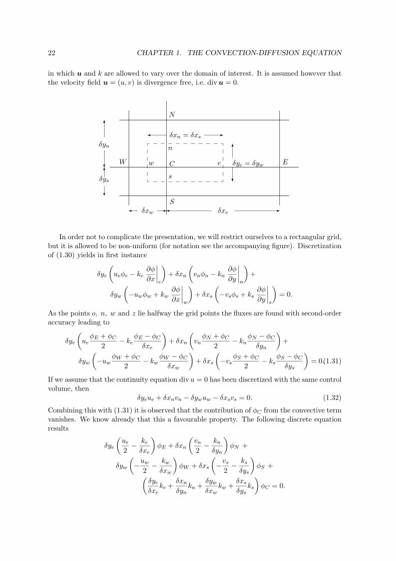
22 CHAPTER 1. THE CONVECTION-DIFFUSION EQUATION
in which u and k are allowed to vary over the domain of interest. It is assumed however thatthe velocity field u = (u, v) is divergence free, i.e. divu = 0.
N
n
W w
S
s
Ee
- -δxw δxe
?
6?
6
δyn
δys
C
-
6
?
δye = δyw
δxn = δxs
In order not to complicate the presentation, we will restrict ourselves to a rectangular grid,but it is allowed to be non-uniform (for notation see the accompanying figure). Discretizationof (1.30) yields in first instance
δye
(ueφe − ke
∂φ
∂x
∣∣∣∣e
)+ δxn
(vnφn − kn
∂φ
∂y
∣∣∣∣n
)+
δyw
(−uwφw + kw
∂φ
∂x
∣∣∣∣w
)+ δxs
(−vsφs + ks
∂φ
∂y
∣∣∣∣s
)= 0.
As the points o, n, w and z lie halfway the grid points the fluxes are found with second-orderaccuracy leading to
δye
(ueφE + φC
2− ke
φE − φCδxe
)+ δxn
(vnφN + φC
2− kn
φN − φCδyn
)+
δyw
(−uw
φW + φC2
− kwφW − φCδxw
)+ δxs
(−vs
φS + φC2
− ksφS − φCδys
)= 0.(1.31)
If we assume that the continuity equation divu = 0 has been discretized with the same controlvolume, then
δyeue + δxnvn − δywuw − δxsvs = 0. (1.32)
Combining this with (1.31) it is observed that the contribution of φC from the convective termvanishes. We know already that this a favourable property. The following discrete equationresults
δye
(ue2− keδxe
)φE + δxn
(vn2− knδyn
)φN +
δyw
(−uw
2− kwδxw
)φW + δxs
(−vs
2− ksδys
)φS +(
δyeδxe
ke +δxnδyn
kn +δywδxw
kw +δxsδys
ks
)φC = 0.

1.7. HIGHER-ORDER SPACE DISCRETIZATION 23
We note that the coefficient of φE depends only on quantities defined in e. When theequation in the neighbouring control volume is constructed, φC in the neighbouring equa-tion obtains the same coefficient, apart from a minus sign in the convective contribution.This makes the contribution of the convective terms skew symmetric, whereas the diffusivecontribution is symmetric. And this is just what one wants!
Remark Generalization of the vertex-centered concept to general grids suggests choosing thecontrol volumes according to a Voronoi tesselation.
1.7 Higher-order space discretization
Inspired by the success of the above second-order symmetry-preserving discretization, inGroningen we have concentrated on their extension to higher-order accuracy. As before, ourchoice of the discretization on non-uniform grids will be explained by studying the convection-diffusion equation. It will be discretized in a finite-volume fashion, as discussed already inSection 1.6, where the control faces are chosen halfway between the grid points (for notationsee Figure 1.2).
i+1 i+2i
h
i−1i−2
h
c
f
Figure 1.2: Fine (hf ) and coarse (hc) control volumes. The volume faces are located halfwaythe grid points (i, i± 1) and (i, i± 2), respectively.
As in Section 1.6, with a second-order flux in xi+1/2 given by
uφi+1 + φi
2− kφi+1 − φi
xi+1 − xi,
the semi-discrete convection-diffusion equation becomes
hfdφidt
+ 12u(φi+1 − φi−1)− k
(φi+1 − φixi+1 − xi
− φi−1 − φixi−1 − xi
)= 0. (1.33)
To turn this method into a fourth-order method, a similar equation on a two-times-largercontrol volume (see Figure 1.2) is written down
hcdφidt
+ 12u(φi+2 − φi−2)− diffusive terms = 0. (1.34)
The leading term in the discretization error can be removed through a Richardson extrapo-lation from (1.33) and (1.34). Since the errors in (1.33) and (1.34) are of third order (notethat these discrete equations are multiplied by h as compared to their usual formulation),on a uniform grid this would mean to make a combination 8*Eq. (1.33)−Eq. (1.34). On anon-uniform grid one would be tempted to tune the weights to the actual mesh sizes, butwe think it important that the skew symmetry of the convective contribution is maintained.

24 CHAPTER 1. THE CONVECTION-DIFFUSION EQUATION
This can only be achieved when the weights are taken independent of the grid location, andhence equal to the uniform weights. In this way the discretization of the convective derivativebecomes
Hi∂φ
∂x≈ 1
2(−φi+2 + 8φi+1 − 8φi−1 + φi−2), (1.35)
whereHi = 8hf − hc = 1
2(−xi+2 + 8xi+1 − 8xi−1 + xi−2).
On a uniform grid, of course, the usual fourth-order method is obtained, but on non-uniformgrids the method differs considerably! In particular, the local truncation error given implicitlyby
2Hi∂φ
∂x= −φi+2 + 8φi+1 − 8φi−1 + φi−2
+ (h2++ − 8h2
+ + 8h2− − h2
−−)φxx + · · ·
(where h++ = xi+2−xi, h+ = xi+1−xi, etc.) does not look very promising at first sight. Onirregular grids it might even behave first-order (instead of fourth-order)!
The diffusive term undergoes a similar treatment leading to
Hi∂2φ
∂x2≈ 8
(φi+1 − φixi+1 − xi
− φi−1 − φixi−1 − xi
)−(φi+2 − φixi+2 − xi
− φi−2 − φixi−2 − xi
). (1.36)
Remark The expressions (1.35) and (1.36) can also be derived through a coordinate trans-formation x = x(ξ) by writing
dφ
dx=
dφ
dξ/
dx
dξand
d2φ
dx2=
d
dξ
(dφ
dξ/
dx
dξ
)/
dx
dξ.
Choose a uniform grid in ξ with mesh size ∆, then
dφ
dξ=−φi+2 + 8φi+1 − 8φi−1 + φi−2
12∆+O(∆4),
dx
dξ=−xi+2 + 8xi+1 − 8xi−1 + xi−2
12∆+O(∆4)
⇒ dφ
dx=−φi+2 + 8φi+1 − 8φi−1 + φi−2
−xi+2 + 8xi+1 − 8xi−1 + xi−2+O(∆4).
Now, fourth-order behaviour looks obvious...
Testcase convection-diffusion
The performance of the above 2nd- and 4th-order methods will be demonstrated by comparingthem with the traditional discretization methods based on Lagrange interpolation (minimisinglocal truncation error). Since on uniform grids the methods are equal, an example witha boundary-layer character is chosen, requiring grid refinement near the outflow boundaryx = 1. Thus, the steady convection-diffusion equation
dφ
dx− kd2φ
dx2= 0 (0 < x < 1) φ(0) = 0, φ(1) = 1 (1.37)

1.7. HIGHER-ORDER SPACE DISCRETIZATION 25
is solved, with a diffusion coefficient equal to k = 0.001.
Two types of grid have been examined. Firstly, we will present results for piecewise-uniform grids where the interval [0, 1] is split into two parts, in each of which the grid is takenuniform. The interface point, denoted by 1−d, is chosen near the edge of the boundary layerwhich has thickness d = O(k). In both parts half of the grid points are positioned. Notethat near the interface point the grid size abruptly changes, and only here the discretizationdiffers from the Lagrangian one. Secondly, we have investigated more smoothly stretchedgrids. Results will be presented for a grid with a constant stretching (obtained through anexponential transformation function), again chosen such that half of the grid points lie in theboundary layer. Four discretization methods have been investigated:
– 2L: The traditional Lagrangian second-order method.
– 2S: The second-order symmetry-preserving method defined by (1.33).
– 4L: The traditional fourth-order Lagrangian method where we have implemented exactboundary conditions to circumvent the problem of a difference molecule that is toolarge near the boundary. In this way the boundary treatment does not interfere withthe internal discretization.
– 4S: In the method defined by (1.35) and (1.36), the problems due to the ‘missing’boundary conditions have been solved by using the second-order discretization (1.33)in the end points.
As the analytical solution to (1.37) is known, we can monitor the global discretization errordefined by ||φh − φexact||h, where the norm is the kinetic energy norm defined in (1.27).
Figure 1.3: The global error as a function of the mean mesh size. Half of the grid pointsis located in the boundary layer of thickness d. Four methods are shown: 2L (second-orderLagrangian), 2S (second-order symmetry-preserving), 4L (fourth-order Lagrangian with exactboundary conditions) and 4S (fourth-order symmetry-preserving with second-order boundarytreatment).

26 CHAPTER 1. THE CONVECTION-DIFFUSION EQUATION
Figure 1.4: The number of eigenvalues located in the (unstable) left halfplane for the La-grangian methods as a function of mean mesh size (2L second-order; 4L fourth-order withexact boundary conditions).
In Fig. 1.3 the global error is presented as a function of the mean mesh size (= 1/N , whereN is the number of grid points). Two abrupt grids have been chosen, one in which d = 5k,which is too narrow to catch the boundary layer accurately, and one with d = 15k. Further,one exponential grid is shown with d = 10k (on a smoothly stretched grid the location of theinterface point is less critical).
A number of observations can be made. Firstly, often the fourth-order Lagrangian methodis not more accurate than its second-order counterpart, especially when the number of gridpoints is not abundant. This explains why thus far fourth-order discretization has not beenvery popular.
Secondly, when the number of grid points is low, Lagrangian discretization is much less ac-curate than symmetry-preserving discretization. Also, on the narrow abrupt grid Lagrangiandiscretization suffers most. In contrast, the symmetry-preserving discretization method be-haves smoothly on all grids; even on the coarsest grids the error does not exceed 10−2.Turbulent-flow simulations will always create the situation where one has to cope with limi-tations on the affordable number of grid points; hence methods that are less sensitive in thisrespect are preferable.
Thirdly, on the exponential grid the fourth-order Lagrangian method nearly breaks downfor N = 28 where the stretching factor is 1.4 (which is large but not extreme). For this classof methods some eigenvalues of the coefficient matrix may be located in the left halfplane.Upon refinement these eigenvalues will cross the imaginary axis, and, for this particular valueof N , one of these eigenvalues almost vanishes, making the system almost singular. Note thatthe symmetry-preserving fourth-order method for this value of N is already very accurate,with an error around 10−5.
When one or more eigenvalues of the coefficient matrix are located in the left halfplane,the semi-discrete system (1.26) is unstable, and cannot be integrated in the time domain;in the above examples the discrete solution has been obtained by a direct matrix solver. Toillustrate how serious this problem is, in Fig. 1.4 the number of eigenvalues that are located inthe unstable left halfplane are presented. Only the Lagrangian methods are shown, since the

1.8. TIME INTEGRATION 27
symmetry-preserving discretization always keeps the eigenvalues in the stable right halfplane.Note that upon grid refinement also all ‘Lagrangian’ eigenvalues will end up in the righthalfplane, since eventually the mesh Peclet numbers will become smaller than 2.
1.8 Time integration
1.8.1 Stability analysis
Before proceeding towards more advanced space discretization methods for the convection-diffusion equation its time integration will be discussed, i.e. we start with the unsteady equa-tion
∂φ
∂t+ u
∂φ
∂x− k ∂
2φ
∂x2= 0, 0 < x < 1. (1.38)
This equation will be discretized explicitly in time and central in space, to obtain
φ(n+1)j − φ(n)
j
δt+ u
φ(n)j+1 − φ
(n)j−1
2h− k
φ(n)j+1 − 2φ
(n)j + φ
(n)j−1
h2= 0.
After introduction of the following abbreviations
η ≡ u δt
h(CFL-number) and d ≡ 2k δt
h2(1.39)
the discrete equation can be rewritten as
φ(n+1)j − φ(n)
j +η
2
(φ
(n)j+1 − φ
(n)j−1
)− d
2
(φ
(n)j+1 − 2φ
(n)j + φ
(n)j−1
)= 0. (1.40)
In case of periodic boundary conditions
φ(0, t) = φ(1, t),
Fourier analysis yields the correct amplification behaviour of the time-integration method (see
Appendix A.3). Thereto φ(n)j = c
(n)θ eijθ is substituted, to find (after division by eijθ)
c(n+1)θ = c
(n)θ
[1 +
d
2
(eiθ − 2 + e−iθ
)− η
2
(eiθ − e−iθ
)]= c
(n)θ [1 + d (cos θ − 1)− iη sin θ] .
The expression between the brackets is the Fourieramplification factor
g(θ) = 1− d (1− cos θ)− i η sin θ. (1.41)
In the complex plane it represents an ellipse withcenter (1− d, 0) and half main axes equal to d andη, respectively.
ηd
1
1
locus of theamplification factor g(θ)

28 CHAPTER 1. THE CONVECTION-DIFFUSION EQUATION
The requirement |g(θ)| ≤ 1 leads to
[1 + d (cos θ − 1)]2 + η2 sin2 θ ≤ 1
⇔ d2(cos θ − 1)2 + 2d (cos θ − 1) + η2(1− cos2 θ) ≤ 0
⇔ d2(1− cos θ)− 2d+ η2(1 + cos θ) ≤ 0
⇔ d2 + η2 − 2d+ (η2 − d2) cos θ ≤ 0. (1.42)
This has to hold for all θ. A simple observation shows that the left-hand side in (1.42) attainsits maximum in either θ = 0 or θ = π. These two values lead to the necessary and sufficientconditions for Fourier stability
η2 ≤ d and 0 ≤ d ≤ 1. (1.43)
The first condition in (1.43) can be rewritten as
η2 ≤ d ⇔ u2δt ≤ 2k ⇔ P ≡ 2η
d≤ 2√
d. (1.44)
We investigate zero-stability (see Appendix A.3) for δt → 0 and h → 0 with d constant.Taking the modulus of (1.41) yields
|g|2 = 1− d (1− cos θ)2 + η2 sin2 θ = 1− d (1− cos θ)2 +u2δt2
h2sin2 θ. (1.45)
The first term (between braces) in the right-hand side is less or equal unity as soon as0 ≤ d ≤ 1. The second term looks small enough anyway, it is even O(δt2), but the factor 1/h2
is misleading. It can become arbitrary large when h → 0. Therefore it has to be ‘tamed’ byone of the factors δt; i.e. δt/h2 should remain bounded. The latter is obviously satisfied whend is bounded, and the desired O(δt) is achieved. Thus, ultimately we find that the scheme iszero-stable when
0 ≤ d ≤ 1, (1.46)
which is a weaker requirement than that for Fourier stability in (1.43). However, the coef-ficient of the δt-term in (1.45) can be large, and herewith |g|. This is a situation which isnot acceptable in practice (as is shown below), and where one uses preferably the strongerconcept of practical Fourier stability (see Appendix A.3).
It is interesting to analyse which of the conditions in (1.43) puts the strongest restrictionon the time step. The diffusive condition d ≤ 1 results in
δt ≤ h2
2k≡ δtdiff ,
whereas rewriting (1.44) gives
δt ≤ δtFour ≡2k
u2=h2
2k
4k2
u2h2= δtdiff
4
P 2.
It follows that for P < 2 the diffusive condition d ≤ 1 is most restrictive, whereas for P > 2the condition η2 ≤ d is most restrictive. A similar comparison holds with the convective

1.8. TIME INTEGRATION 29
condition η ≤ 1 which we would have encountered when upwind discretization would havebeen applied (see the example in Appendix A.3.4):
η ≤ 1 ⇔ δt ≤ δtconv ≡h
u=h2
2k
2k
hu= δtdiff
2
P.
A final aspect to investigate is the positivity of the discrete operator. Hereto the coef-ficients of all neighbouring points (in space as well as in time) have to be considered. Iteasily follows that the discrete operator in our problem is a positive operator if and only ifd ≤ 1 ∧ P ≤ 2: a requirement which is stronger than (1.43).
1.8.2 Practical example
When mixed Dirichlet/Neumann boundary conditions
φ(0, t) = given;∂φ
∂x(1, t) = given, (1.47)
are applied, in Section 1.11 the matrix method predicts absolute stability under the conditions
[η2 ≤ d2 ∧ d+√d2 − η2 ≤ 2] ∨ [d2 ≤ η2 ≤ 2d]. (1.48)
In the adjacent figure the various stability regionshave been indicated. In the ‘white’ area in the bottom-left corner the operator is positive; the discrete solu-tion does not show any wiggles. The requirement ofabsolute stability for periodic boundary conditions al-lows the doubly shaded area top left. Here the time-integration method is practical (Fourier) stable. Zero-stability increases the allowable region to the stripd ≤ 1. Also the Dirichlet–Neumann conditions in-crease the region of absolute stability; this time withthe singly-shaded region given by (1.48).
s s ss s
s s s4
2
00 1 2d ∼ δt
P ∼ h
D E F
A B C
G H
...................................................................
@@@@@@@@@@@
@@@
@@
Next we will show what the discrete solution looks like for various choices of δt and h.The equation (1.38) is solved for u = 2 and k = 0.05, with homogeneous Dirichlet–Neumannboundary conditions (1.47). As initial condition φ(x, 0) = x is chosen. Three choices for thegrid size have been made: h = 1/10, 1/20 and 1/40. At each of these grid sizes the discretesolution has been determined for a number of choices for the time step δt. The various caseshave been indicated in the figure with the letters A through H.
The behaviour of the discrete solution as a function of time is shown by plotting φ(1, t),i.e. the value at the Neumann boundary, for 0 ≤ t ≤ 4.
• Cases A, B and C possess a grid size h = 1/10. For A the time step has been selectedsuch that the scheme is absolutely and practically stable for periodic boundary condi-tions. In B there is only absolute stability with D–N conditions, and in C there is noabsolute stability. For each of these cases the scheme is zero-stable. All three solutionsshow oscillations (we are outside the area where the solution should be wiggle-free).Case A with δt = 0.02 looks quite nice, case C is unacceptable.

30 CHAPTER 1. THE CONVECTION-DIFFUSION EQUATION
0
0.5
1
0 1 2 3 4t
φ A
A : h = 1/10; δt = 0.02(A+ N + P+)
0
0.5
1
0 1 2 3 4t
φ B
B : h = 1/10; δt = 0.04(A+ N + P−)
0
0.5
1
0 1 2 3 4t
φ C
C : h = 1/10; δt = 0.055(A− N + P−)
0
0.5
1
0 1 2 3 4t
φ D
D : h = 1/20; δt = 0.02(A+ N + P+)
-10
0
10
0 1 2 3 4t
φ E
E : h = 1/20; δt = 0.03(A+ N − P−)
-1e+09
0
1e+09
0 1 2 3 4t
φ F
F : h = 1/20; δt = 0.04(A+ N − P−)
0
0.5
1
0 1 2 3 4t
φ G
G : h = 1/40; δt = 0.005(A+ N + P+)
-0.5
0
0.5
1
0 1 2 3 4t
φH
H : h = 1/40; δt = 0.00655(A+ N − P−)
Between parentheses + and − indicate whether for this choice of δt and h the time-integration
method possesses absolute stability (A), zero-stability (N) and/or practical stability (P ).
• In the cases D, E and F the grid size equals h = 1/20. In D a positive operator iscreated, which is absolutely, practically and zero-stable; the solution is monotone. Eand F are only absolutely stable with D–N conditions. An instability develops, whichafter some time (when the Dirichlet condition becomes manifest) is being damped. Butin the mean time the solution has been growing quite a bit (in F : 109). In linear-algebraterms, this (almost ‘fatal’) instability is due to (large) Jordan blocks which cause analgebraic growth; see the growth-estimate (A.16).
• In G and H the grid size equals h = 1/40. Case G satisfies all stability conditionsand produces a nice solution. Case H is just outside the region of zero stability; thisstability boundary is at δt = 0.00625. Just as in cases E and F an instability developswhich eventually gets damped.
The time step in case H is δt = 0.00655; this is a factor of three smaller than in cases Aand D. With respect to accuracy the latter cases are quite good and the larger time stepapparently is small enough. The fact that in cases H and G a much smaller time step has tobe chosen is dictated by the stability of the method, rather than by its accuracy.

1.9. BURGERS’ EQUATION – DISCONTINUOUS SOLUTIONS 31
In conclusion it is remarked that the three best-looking solutions A, D and G preciselycorrespond with the cases where the time-integration method satisfies the criteria for practicalstability, herewith illustrating the usefulness of this notion.
1.9 Burgers’ equation – discontinuous solutions
In this section a first step is made towards solving the compressible Navier–Stokes equations.The main difference between the compressible and the incompressible equations is the possi-bility for discontinuities – shock waves – to develop in the solution. Using the one-dimensionalequation of Burgers as a model, either in non-conservation form
∂u
∂t+ u
∂u
∂x= 0, (1.49)
or in conservation form∂u
∂t+
∂
∂x(1
2u2) = 0, (1.50)
the performance of the thus far treated discrete approximation methods on non-smooth so-lutions will be demonstrated.
Finite-volume discretization
In Section 1.6 we have already encountered the finite-volume method (FVM) for the dis-cretization of a conservation law like∫∫
Ω
∂u
∂tdΩ +
∫ΓF (u) · n dΓ = 0. (1.51)
Consider this approach in a one-dimensional situation on a uniform grid as shown here:
u ppuui− 1 i i+ 1
+
F (u)|i+1/2
h -
The flux through the right-hand face of the control ‘volume’ around the point i is computedas
F (u)|i+1/2 := F (ui+1/2) = F (12(ui + ui+1)), (1.52)
in which the value of u on this face is found through averaging the neighbouring cell valuesof u. For the discretization of the term ∂F/∂x in the differential equation corresponding to(1.51)
∂u
∂t+ divF (u) = 0, (1.53)
this implies∂F
∂x≈F (ui+1/2)− F (ui−1/2)
h. (1.54)
As an alternative to (1.52), we could have averaged F (u)|i+1/2 from neighbouring valuesof F (u):
F (u)|i+1/2 := 12F (ui) + F (ui+1). (1.55)

32 CHAPTER 1. THE CONVECTION-DIFFUSION EQUATION
This results in the discretization
∂F
∂x≈ F (ui+1)− F (ui−1)
2h, (1.56)
where a central finite-difference (FDM) discretization is recognised. In Section 2.3 it is demon-strated that the choice (1.52) is to be preferred, as in the Navier–Stokes equations it corre-sponds with (2.19′) which leads to a skew-symmetric discretization of convection.
An upwind-biased choice of the flux is given by F (u)|i+1/2 := F (ui) (for u > 0), leadingto the upwind discretization
∂F
∂x≈ F (ui)− F (ui−1)
h. (1.57)
Burgers’ equation
We will study Burgers’ equation (named after Johannes Marinus Burgers, a Delft professorof fluid dynamics) in a situation with shock waves. In order to obtain the correct analyticalshock solution it is necessary to employ the conservation form (1.50). It is known that thepropagation speed S of a discontinuity in its solution is given by
−S[u] + [12u
2] = 0, (1.58)
where [·] is the jump of the argument across the discontinuity. For Burgers’ equation thisresults in
S = 12(uLeft + uRight). (1.59)
As initial condition we choose
x ≤ 0 : u = 1; 0 ≤ x ≤ 1 : u = 1− x; 1 ≤ x : u = 0.
The characteristics of Burgers’ equation, along which u = Constant, have a slope dx/dt = u.As uLeft > uRight the waves from the left overtake the other ones and a shock wave is created,with a shock speed S = 1
2 as follows from (1.59). The analytic solution is shown below.
6u
>
-x
t
((((((((((((((((((( ((((
((((((((
(((
((((((((
((((
PPPPPPPPPP
HHHHHHH
ZZZZZ
SSSS
Discretization
We will now solve Burgers’ equation by several discretization methods, globally distinguishedas i) upwind or ii) central (with or without explicitly added diffusion). Moreover, both theconservative form (1.50) and the non-conservative form (1.49) will be considered. Forward

1.9. BURGERS’ EQUATION – DISCONTINUOUS SOLUTIONS 33
Euler is used as time integrator. For all computations the mesh size in x-direction has beenchosen as h = 1/10 with a time step δt = 1/40; the CFL-number becomes η ≡ u δt/h ≤ 1/4.Since there is no diffusion, the mesh-Peclet number P ≡ uh/k is infinite.
In the table below the various discretizations for the convective terms are summarised
non-conservation form conservation form
upwind FDM/FVM uiui−ui−1
h
12u2i−
12u2i−1
h
central FDM uiui+1−ui−1
2h
12u2i+1−
12u2i−1
2h
central FVM not applicable12u2i+1/2
− 12u2i−1/2
h
Below it will be shown that the difference between both columns is essential. The differencebetween both central methods in the right-hand column is less important; both are a discreteconservation law, only the flux computation is slightly different – compare (1.52) with (1.55).
In Section 1.8 the stability of centrally-discretized convection-diffusion equations has beenstudied. Next to the CFL-number η, the quantity d ≡ 2k δt/h2 has been introduced. It wasdemonstrated that forward Euler is zero-stable if and only if d ≤ 1. Practical stability isachieved for (see (1.43)) η2 ≤ d ≤ 1, whereas for Dirichlet/Neumann conditions the regionwith absolute stability is larger than that of practical stability. Without diffusion d = 0,hence central discretization is always zero-stable. At the same time, for no choice of δt > 0the criterion η2 ≤ d can be satisfied (unless u = 0), hence there is no practical stability.
Discrete solution
Let us first observe the difference between upwind discretization and central discretization.The upwind solution is smooth, as was to be expected from the theory of positive operators.The practical stability limit is CFL = 1 which is clearly satisfied.
Remark As u is not constant we cannot perform the ‘accuracy trick for upwind’ CFL ≡ 1(see the example in Section A.3.4).
Clearly visible in the central solution are the strongly growing oscillations induced by thesteep gradient. If we want to suppress these, numerical diffusion has to be added explicitly.Its influence is investigated with ka = 1/20, chosen such that for u ≤ 1 the mesh-Pecletnumber satisfies P ≤ 2. Further it follows that d = 1/4, hence the time integration is stableunder all definitions (we are in the blank bottom-left area in the figure on page 29). As ex-pected theoretically, all oscillations have disappeared, but the discontinuity has been smearedout excessively. Note that in regions with low values of u, this amount of viscosity is muchlarger than the upwind viscosity (which scales with u). In this respect, upwind isn’t that bad...
Next, observe the propagation speed of the shock. In both solutions of the non-conservationform (1.49) the shock does not move; the solutions of the conservation form do have a propershock speed. This holds for both upwind and central solutions. It is concluded that analyticjump conditions, like (1.58), only correctly carry over to the discrete form if we start from the
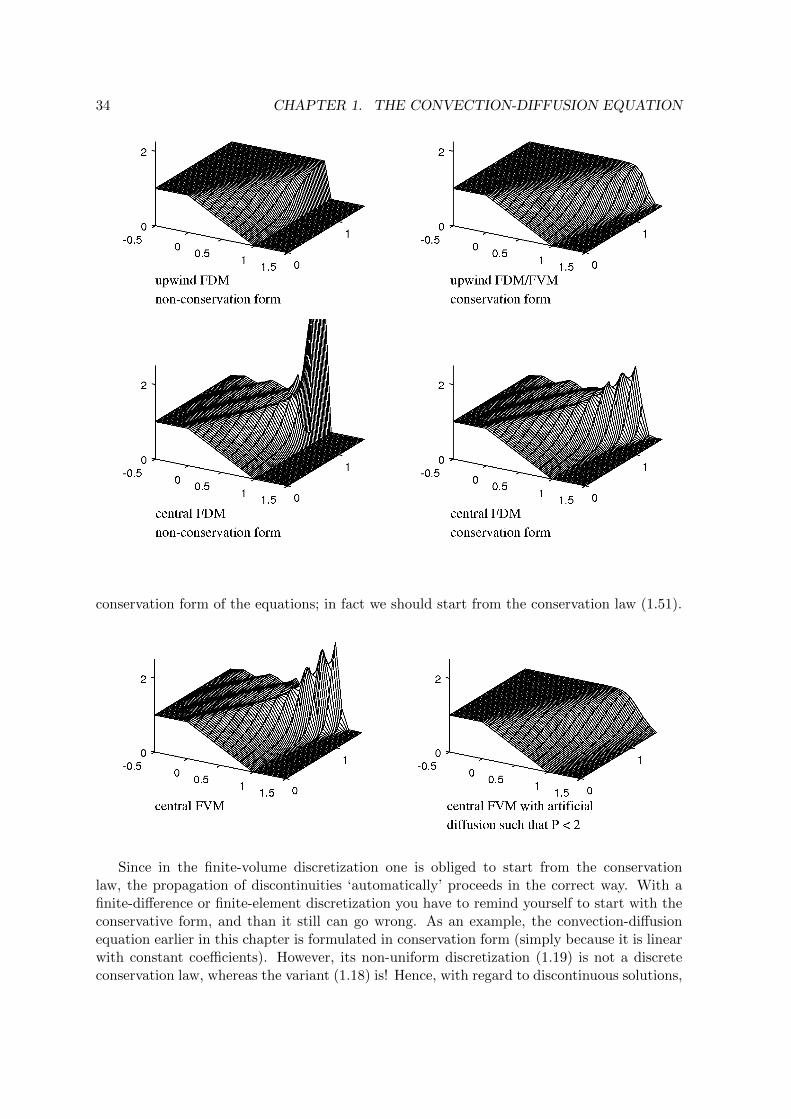
34 CHAPTER 1. THE CONVECTION-DIFFUSION EQUATION
conservation form of the equations; in fact we should start from the conservation law (1.51).
Since in the finite-volume discretization one is obliged to start from the conservationlaw, the propagation of discontinuities ‘automatically’ proceeds in the correct way. With afinite-difference or finite-element discretization you have to remind yourself to start with theconservative form, and than it still can go wrong. As an example, the convection-diffusionequation earlier in this chapter is formulated in conservation form (simply because it is linearwith constant coefficients). However, its non-uniform discretization (1.19) is not a discreteconservation law, whereas the variant (1.18) is! Hence, with regard to discontinuous solutions,

1.10. ‘CONVECTIVE’ CONCLUSIONS 35
the finite-volume discretization is essentially different from the other discretization methods.
The above figures clearly show the influence of using the conservation form or not (left:no, right: yes). The figure below shows the central FVM (by definition in conservation form)with and without adding numerical diffusion. It will be clear that the discrete solutionsfor discontinuous solutions are not yet really convincing. Therefore special methods havebeen developed, e.g. based on the concept of (nonlinear) limiters, to reduce the amount ofoscillations in the solution. The monograph by Hirsch (1990) gives a nice introduction intothis subject.
1.10 ‘Convective’ conclusions
It has been demonstrated that the discretization of convection, just a ‘simple’ first-orderderivative, is very subtle. The major problem with the discretization is that, through itsdiscretization error, it interferes with diffusion: sometimes this poses no serious harm, butsometimes it can also be devastating to the quality of the numerical solution. It is impossibleto give general guidelines, yet I would like to do so.
The question to ask is:
“Is diffusion critical to the flow problem?”
Depending upon the answer, two situations arise:
Yes, diffusion is critical In this case it is necessary to resolve all boundary layers throughgrid refinement. Further, convection is preferably discretized with skew-symmetricmethods.
No, diffusion is not critical In this case diffusion could be neglected (to obtain the Eulerequations), but also there is no problem with (limited) increasing diffusion. Boundarylayers do not have to be resolved, and upwind-biased discretization of convection (im-plicitly adding numerical diffusion) is applicable; explicit addition of diffusion is suitableas well. If necessary, to retain sharp discontinuities or to further suppress oscillations,limiters may be applied.
1.11 Appendix: Dirichlet–Neumann stability analysis
We will here6 give the details of the stability analysis of (1.40) under mixed Dirichlet–Neumann conditions
φ(0, t) = given and∂φ
∂x(1, t) = given.
(1.40) combined with these boundary conditions can be written in following matrix notation
2I φ(n+1) = (2I −A)φ(n) (1.60)
6This section is taken from P. Wesseling and P. Wilders (1984) Numerieke Stromingsleer A, Lecture Notesa110A (in Dutch), TU Delft.

36 CHAPTER 1. THE CONVECTION-DIFFUSION EQUATION
with
A =
2d η − d−η − d 2d η − d
. . .
−η − d 2d η − d−2d 2d
←− here the Dirichlet conditionhas been substituted
←− the Neumann condition
(1.61)
We need two lemmas. The first lemma introduces a similarity transformation with which A can be trans-formed into either a symmetric matrix or the sum of a constant diagonal matrix and a skew-symmetric matrix.The second lemma gives an estimate for the eigenvalues of this type of matrices. We remark that Lemma 1implies that A is non-defect.
Lemma 1 Let A be a tridiagonal matrix with
aii = αi (i = 1, . . . , k);
ai+1,i = γi+1, ai,i+1 = βi+1, γi 6= 0, βi 6= 0 (i = 1, . . . , k − 1).
Let D be a diagonal matrix with
d11 = 1, dii = di−1,i−1
√∣∣∣∣γiβi∣∣∣∣ (i = 2, . . . , k).
Let B = D−1AD. Then B is tridiagonal with
bii = αi (i = 1, . . . , k);
bi+1,i = sgn (γi+1)√|βi+1γi+1|
bi,i+1 = sgn (βi+1)√|βi+1γi+1|
(i = 1, . . . , k − 1).
Proof Is left to the reader. 2
Lemma 2 Let B be a tridiagonal k × k matrix with
bii = d (i = 1, . . . , k);
|bi+1,i| = |bi,i+1| = b (i = 1, . . . , k − 2);
|bk,k−1| = |bk−1,k| = γ where γ ≤ b√
2.
Then each eigenvalue µ of B satisfies |µ− d| ≤ 2b.
Proof Let D be a diagonal matrix with dii = 1 (i = 1, . . . , k − 1), and dkk = b/γ. Let C = D−1BD.We have cij = bij , (i, j) 6= (k, k − 1), (k − 1, k) and ck,k−1 = γ
bbk,k−1 en ck−1,k = b
γbk−1,k. On C Gerschgorin’s
theorem can be applied from which the lemma follows immediately. 2
We can now proceed to estimating the eigenvalues of the matrix A from (1.61). When η2 6= d2 thetransformation from Lemma 1 is applicable. The resulting matrix B becomes
bii = 2d (i = 1, . . . , k);
bi,i+1 = sgn (η − d)√|d2 − η2| , (i = 1, . . . , k − 2);
bi+1,i = sgn (−η − d)√|d2 − η2| , (i = 1, . . . , k − 2);
bk−1,k = sgn (η − d)√
2d |d− η| ;
bk,k−1 = sgn (−2d)√
2d |d− η|.
Since η ≥ 0 we have √2d |d− η| ≤
√2(d+ η) |d− η| =
√2√|d2 − η2|,
with which the matrix B satisfies the conditions from Lemma 2. We remark that the matrices A and B fromLemma 1 possess the same eigenvalues
µ = µR + iµI .

1.12. REFERENCES 37
– For d2 > η2 the matrix B is symmetrical. The eigenvalues µ of B (and of A) are real and, according toLemma 2, satisfy
2d− 2√d2 − η2 ≤ µR ≤ 2d+ 2
√d2 − η2, µI = 0.
– For d2 < η2 we have B = 2dI+ B, where B is skew symmetric. The eigenvalues of B are purely imaginary.Lemma 2 is applicable to B, which yields
µR = 2d, 0 ≤ µI ≤ 2√η2 − d2. (1.62)
Absolute stability requires all eigenvalues λ of the iteration matrix (I − 12A) from (1.60) to satisfy |λ| ≤ 1.
I.e. the eigenvalues of A (and B) have to satisfy
|1− 12µ| ≤ 1 ⇔ µ2
R + µ2I − 4µR ≤ 0. (1.63)
– For d2 > η2 we have µI = 0, after which we only have to show that 0 ≤ µR ≤ 4. From (1.62) it followssimply that
d+√d2 − η2 ≤ 2
is a sufficient condition to satisfy (1.63).– For d2 < η2 we have µR = 2d. The estimate (1.62) now yields that
η2 ≤ 2d
is a sufficient condition for (1.63) to hold.
Herewith the statement in (1.48) has been proven. Moreover it is clear, from a comparison with (1.43), thatthe Dirichlet-Neumann conditions yield additional stability in comparison with periodic boundary conditions.
1.12 References
D.N. de G. Allen and R.V. Southwell (1955) Relaxation methods applied to determine the motion intwo dimensions of a viscous fluid past a fixed cylinder. Quart. J. Mech. Appl. Math. 8, 129
P.M. Gresho and R.L. Lee (1981) Don’t suppress the wiggles - they are telling you something. Comput.Fluids 9, 223–253.
A.C. Hindmarsch, P.M. Gresho and D.F. Griffiths (1984) The stability of explicit Euler time-integrationfor certain finite difference approximations of the multi-dimensional advection-diffusion equa-tion. Int. J. Num. Meth. Fluids 4, 853–897.
C. Hirsch (1990) Numerical Computation of Internal and External Flows, Volume 2. John Wiley.
A. Jameson, W. Schmidt and E. Turkel (1981) Numerical solutions of the Euler equations by finite-volume methods using Runge–Kutta time-stepping schemes. AIAA paper 81-1259.
B.P. Leonard (1979) A stable and accurate convective modelling procedure based on quadraticupstream interpolation. Comput. Meth. Appl. Mech. Eng. 19, 59–98.
B.P. Leonard and J.E. Drummond (1995) Why you should not use ’hybrid’, ’power-law’ or relatedexponential schemes for convective modelling - there are much better alternatives. Int. J. Num.Meth. Fluids 20, 421–442.
T.A. Manteuffel and A.B. White Jr. (1986) The numerical solution of second-order boundary valueproblems on nonuniform meshes. Math. Comput. 47, 511–535.
R.D. Richtmyer and K.W. Morton (1967) Difference Methods for Initial Value Problems. John Wiley.
D. Spalding (1972) A novel finite-difference formulation for differential expressions involving bothfirst and second derivatives. Int. J. Num. Meth. Eng. 4, 551–559.
A.E.P. Veldman and E.F.F. Botta (1993) Grid quality - an interplay of grid and solver. In: M.J.Baines and K.W Morton (eds.) Numerical Methods for Fluid Dynamics 4. Oxford UniversityPress, 329–335.

38 CHAPTER 1. THE CONVECTION-DIFFUSION EQUATION
A.E.P. Veldman and K. Rinzema (1991) Playing with nonuniform grids, J. Eng. Math. 26, 119–130.
R.W.C.P. Verstappen and A.E.P. Veldman (1997) Direct numerical simulation of turbulence at lowercosts. J. Eng. Math. 32, 143–159.
R.W.C.P. Verstappen and A.E.P. Veldman (1998) Spectro-consistent discretization: a challenge toRANS and LES. J. Eng. Math. 34, 163–179.
R.W.C.P. Verstappen and A.E.P. Veldman (2003) Symmetry-preserving discretization for turbulentflow. J. Comput. Phys. 187, 343–368.
P. Wesseling (2001) Principles of Computational Fluid Dynamics. Springer Verlag.
F.W. Wubs and J. Thies (2011) A robust two-level incomplete factorization for (Navier–)Stokessaddle point matrices. SIAM J. Matrix Anal. Appl. 32, 1475–1499.

Chapter 2
Incompressible Navier–Stokesequations
2.1 The equations for fluid flow
The equations of fluid flow are governed by conservation laws for mass, momentum andenergy, completed by a number of thermodynamic relations. The conservation law of mass ina volume Ω reads ∫
Ω
∂ρ
∂tdΩ +
∫Γρu · ndΓ = 0, (2.1)
where ρ denotes the density of the fluid. Conservation of momentum can be written as∫Ω
∂ρu
∂tdΩ +
∫Γρuu · ndΓ =
∫Γσ · ndΓ, (2.2)
where σ = −pI+τ is the internal stress tensor, with p the pressure. The viscous stress tensorτ is defined through
τ = µ[∇u+ (∇u)∗ − 23(∇ · u) I],
with µ the dynamic viscosity of the fluid. The conservation law of energy E = e + 12u · u
reads ∫Ω
∂ρE
∂tdΩ +
∫ΓρE u · ndΓ =
∫Γ(σ · u) · ndΓ +
∫Γk∂T
∂ndΓ,
where heat transport due to temperature (T ) differences has been modelled by Fourier’s law,with k being the thermal conductivity coefficient. Finally, two thermodynamic relations areapplicable
p = ρRT and e = cvT,
where R = cp−cv is the universal gas constant, and cp and cv are the specific heat coefficients.
Several dimensionless parameters are associated with fluid flow. For viscous flow the mostimportant one is the Reynolds number, named after Osborne Reynolds (1842-1912). It isdefined by Re = ρUL/µ, where U is a characteristic velocity of the flow and L a characteristiclength scale. Roughly, this number indicates the relevance of viscous effects in the flow: thelarger Re, the less influence viscosity has on the flow. In this vain, the Reynolds numberforms a useful indicator for the onset of turbulence (see Chapter 3).
39

40 CHAPTER 2. INCOMPRESSIBLE NAVIER–STOKES EQUATIONS
Differential form By applying Gauss’ theorem, the above conservation laws can be trans-formed into differential equations. In particular, conservation of mass (2.1) and momentum(2.2) can be reformulated as
∂ρ
∂t+∇ · (ρu) = 0 (2.3)
and∂ρu
∂t+∇ · (ρuu) = −∇ p+∇ · τ . (2.4)
By combining both equations, conservation of momentum can also be written in the non-conservative form
ρ∂u
∂t+ ρu · ∇u = −∇ p+∇ · τ . (2.4′)
Incompressible flow
In these lecture notes we will focus on incompressible flow. In this case, effectively the energyequation is replaced by the condition of incompressibility
Dρ
Dt≡ ∂ρ
∂t+ u · ∇ ρ = 0,
i.e. the density of a given particle remains constant during its motion (note that in principlethe density does not have to be the same everywhere in the flow). This condition can becombined with the conservation of mass in differential form (2.3) to conclude that the velocityfield is divergence free1
divu = 0. (2.5)
The stress tensor τ now can be simplified, and when moreover ρ and µ are assumed constant,the momentum equation (2.4′) becomes
∂u
∂t+ (u · grad)u = −1
ρgrad p+ ν div gradu, (2.6)
where ν = µ/ρ is the kinematic viscosity. It is remarked that under the incompressibilityconstraint (2.5), the convective term can be written as (u · grad)u = div(uu). Now themomentum equation can again be denoted in conservation form
∂u
∂t+ div(uu) = −1
ρgrad p+ ν div gradu. (2.6′)
When an internal flow is simulated in a domain Ω with a solid boundary Γ only a boundarycondition for the velocity u can be formulated. Usually this will be
u = 0 on Γ. (2.7)
This boundary condition describes two physical effects. Firstly, the impenetrability of thewall requires the normal velocity to vanish. Secondly, the (viscous) shear stress requires thetangential velocity component to vanish (no-slip condition).
1From now on we will use the notation ‘div’ and ‘grad’ instead of the ‘∇’-notation.

2.2. CHOICE OF THE COMPUTATIONAL GRID 41
Acoustical degeneration
Heuristically there does not seem to be an equation for the pressure, unlike in the compress-ible case. It is natural to consider the momentum equation as an equation for the velocity.In the compressible case the continuity equation is an equation for the density, whereas thepressure then follows through an equation of state. In the incompressible case the densitydoes not appear in the continuity equation (2.5), and neither does the pressure. But of course(2.5)+(2.6) together determine velocity and pressure.
To get a feeling for what is going on, we will first consider the one-dimensional isentropicEuler equations
∂ρ
∂t+
∂
∂x(ρu) = 0,
∂u
∂t+ u
∂u
∂x+
1
ρ
∂p
∂x= 0,
(2.8)
where pressure and density are related through
p = p(ρ) withdp
dρ= c2 > 0, (2.9)
in which c is the velocity of sound. Substitution of the p-ρ relation (2.9) in (2.8) yields∂ρ
∂t+ ρ
∂u
∂x+ u
∂ρ
∂x= 0,
∂u
∂t+ u
∂u
∂x+
c2
ρ
∂ρ
∂x= 0.
(2.10)
This system of equations possesses the characteristic directions (found by diagonalizing thecoefficient matrix; see any book on partial differential equations)
dx
dt= u+ c and u− c.
Both directions are real, hence the system is hyperbolic. In the incompressible limit we havec → ∞, therefore the two characteristic directions dx/dt approach ±∞, and hence coincidein the limit with the x-axis and with each other.
The theory on partial differential equations now tells us that the system is degenerating.The acoustical part of the equations, the combination of divu and grad p, is responsible forthis behaviour. Disturbances in the pressure are instantaneously noted everywhere in thedomain. This infinite propagation speed will force us to treat the acoustical part of theNavier–Stokes equations in an implicit manner, as we will see in the sequel.
2.2 Choice of the computational grid
We will start the numerical treatment with a discussion of the spatial discretization. Forconvenience only rectangular domains Ω will be considered, covered by a uniform grid Ω.The grid cells are positioned such that the cell faces coincide with the boundary Γ of Ω. Itseems obvious to define the unknown variables u = (u, v) and p in the corners of the grid cells.However, there are some snakes in the grass. This is not only the case in finite-difference orfinite-volume discretizations, but also in a finite-element approach.

42 CHAPTER 2. INCOMPRESSIBLE NAVIER–STOKES EQUATIONS
A: u, v and p in corner points
When u, v and p are defined in the corner points of the grid cells, it is obvious to applythe momentum equations in these corner points too. For second-order accuracy, the discreteversion of grad p, which we shall denote by Gp, should be computed with central differences.For the grid point indicated with 2 this implies that values of p are used from grid pointsindicated by (for ∂p/∂x) and × (for ∂p/∂y). In this discretization it is possible to con-struct a p 6= Constant for which Gp = 0. To each solution p this p can be added withoutany consequences for the equations of motion. Moreover there is the danger that during thecomputations one encounters (4-fold) singular matrices (i.e. dim Ker(G) = 4), which reflectthis non-uniqueness of the solution.
x
x
2d dΩ
Γ
d
d
d
d
d
d
2
2
2
2
2
2
2
2
2
x x x
x x x
4
4
4
4
In the above figures, the grid points have been divided into 4 groups: 2, , × and 4.Choose p such that in each of the groups p is constant, but the 4 constants are allowed to bearbitrary. Then in a discrete sense Gp = 0, while p shows oscillating behaviour.
Again we encounter an example of odd/even decoupling, caused by discretizing a first-order derivative over two grid cells. When p itself, and not just its gradient, is relevant tothe problem (e.g. one would like to know forces exerted on the solid walls), then some kindof averaging has to be applied to remove the non-physical oscillations. This is not very elegant.
In spite of the above drawback, this spatial positioning is often used, especially for com-pressible flow. Its advantage is that all flow variables (velocity components, pressure, density,temperature, etc.) are defined at the same location. Thus relations between these variables,for instance the thermodynamic relations, are easily implemented without complicated aver-aging procedures. However, to overcome the above decoupling of the pressure a price has tobe paid, for instance some form of artificial ‘pressure diffusion’ (e.g. Rhie and Chow 1983).An alternative is to filter out the pressure component that lies in Ker(G).
B: u and v in corner points, p in cell centres
An alternative is to define p in the centres of the grid cells. In the momentum equationapplied in the point •, second-order discretization of grad p leads to
∂p
∂x≈ 1
2
pNE − pNW
hx+pSE − pSW
hx
=
1
2hxpNE − pSW + pSE − pNW ,
∂p
∂y≈ 1
2
pNE − pSE
hy+pNW − pSW
hy
=
1
2hypNE − pSW − pSE + pNW . (2.11)
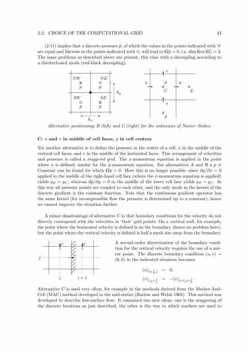
2.2. CHOICE OF THE COMPUTATIONAL GRID 43
(2.11) implies that a discrete pressure p, of which the values in the points indicated with×are equal and likewise in the points indicated with , will lead toGp = 0, i.e. dim Ker(G) = 2.The same problems as described above are present, this time with a decoupling according toa checkerboard mode (red-black decoupling).
6
?
-
hy
hx
x
x
•
p
p
p
p
NW
SE
NE
SW
x x
x
--
6
6
E
S
C
p u
v
u
v
Alternative positionings B (left) and C (right) for the unknowns of Navier–Stokes.
C: u and v in middle of cell faces, p in cell centres
Yet another alternative is to define the pressure in the centre of a cell, u in the middle of thevertical cell faces, and v in the middle of the horizontal faces. This arrangement of velocitiesand pressure is called a staggered grid. The x-momentum equation is applied in the pointwhere u is defined; similar for the y-momentum equation. For alternatives A and B a p 6=Constant can be found for which Gp = 0. Here this is no longer possible, since ∂p/∂x = 0applied in the middle of the right-hand cell face (where the x-momentum equation is applied)yields pE = pC , whereas ∂p/∂y = 0 in the middle of the lower cell face yields pS = pC . Inthis way all pressure points are coupled to each other, and the only mode in the kernel of thediscrete gradient is the constant function. Note that the continuous gradient operator hasthe same kernel (for incompressible flow the pressure is determined up to a constant), hencewe cannot improve the situation further.
A minor disadvantage of alternative C is that boundary conditions for the velocity do notdirectly correspond with the velocities in ‘their’ grid points. On a vertical wall, for example,the point where the horizontal velocity is defined is on the boundary (hence no problem here),but the point where the vertical velocity is defined is half a mesh size away from the boundary.
-
6 6v v
uj
i i+ 1
A second-order discretization of the boundary condi-tion for the vertical velocity requires the use of a mir-ror point. The discrete boundary condition (u, v) =(0, 0) in the indicated situation becomes
(u)i+ 12,j = 0,
(v)i,j+ 12
= −(v)i+1,j+ 12.
Alternative C is used very often, for example in the methods derived from the Marker-And-Cell (MAC) method developed in the mid-sixties (Harlow and Welsh 1965). This method wasdeveloped to describe free-surface flow. It contained two new ideas: one is the staggering ofthe discrete locations as just described, the other is the way in which markers are used to

44 CHAPTER 2. INCOMPRESSIBLE NAVIER–STOKES EQUATIONS
keep track of the liquid. The latter idea gave the method its name. Another early applicationis in meteorology (e.g. Arakawa 1966), where the three above schemes are known as ArakawaA, B and C, respectively.
2.3 Discretization - explicit
In the sequel the computational grid from the MAC method (alternative C) will be used.However, this does not imply that both other alternatives do not have reason for existence(for example on non-orthogonal grids). The grids remain uniform for ease of presentation.
First the equations of motion (2.5)+(2.6) will be written in a more schematic form
divu = 0, (2.12)
∂u
∂t+ grad p = R, (2.13)
where p/ρ is replaced by p (i.e. ρ is normalized at 1). Further
R = −(u · grad)u+ ν div gradu (2.14)
contains all convective and diffusive forces; if desired, also a body force can be included.
In this section, again for simplicity, an explicit time-integration method with two timelevels is applied:
divu(n+1) = 0, (2.15)
u(n+1) − u(n)
δt+ grad p(n+1) = R(n). (2.16)
Equation (2.15) and grad p in (2.16) havereceived an index n + 1 to indicate that theu(n+1) that follows from (2.16) is divergencefree. In fact, the constraint (2.15) determinesthe pressure p(n+1): p is the Lagrange multipliercorresponding with this constraint.
For the discretization in space the followingschemes are applied (for notation see accompa-nying figure):
.
.
.
.
.
.
.
.
.
.
.
.
.
.
.
.
.
.
.
.
.
.
.
.
.
.
.
.
.
.
.
.
.
.
.
.
.
.
.
.
.
.
.
.
.
.
.
.
.
.
.
.
.
.
.
.
.
.
.
.
.
.
.
.
.
.
.
.
.
.
.
.
.
.
.
.
.
.
.
.
.
.
.
.
.
.
.
.
.
.
.
.
.
.
.
.
.
.
.
.
.
.
.
.
.
.
.
.
.
.
.
.
.
.
.
.
.
.
.
.
.
.
.
.
.
.
.
.
.
.
.
.
.
.
.
.
.
.
.
.
.
.
.
.
.
.
.
.
.
.
.
.
.
.
.
.
.
.
.
.
.
.
.
.
.
.
.
.
.
.
.
.
.
.
.
.
.
.
.
.
.
6
6
6
6
- - -
-
-
• •
•
•
S
SW s SE
W w C e E
NW n NE
N
Continuity equation
The continuity equation (2.15) is applied in cell centres. In a natural way it can be discretizedcentrally. The eastern cell with centre e gives a discrete finite-volume conservation law
u(n+1)E hy + v
(n+1)NE hx − u(n+1)
C hy − v(n+1)SE hx = 0. (2.17)
In finite-difference notation it reads
u(n+1)E − u(n+1)
C
hx+v
(n+1)NE − v(n+1)
SE
hy= 0. (2.17′)

2.3. DISCRETIZATION - EXPLICIT 45
Observe that the number of continuity equations equals the number of grid cells. Also thenumber of pressure unknowns equals the number of cells. Hence, there are as many discretecontinuity equations as unknown pressure values! Note that this equality does not hold forpositioning methods A and B.
Momentum equation: convection
The x-momentum equation is applied in the midpoints of the vertical cell faces. In the pointC we obtain (in finite-difference notation)
u(n+1)C − u(n)
C
δt+p
(n+1)e − p(n+1)
w
hx= R
(n)C , (2.18)
where the pressure gradient has been discretized centrally. The term RC contains derivativesfor the convective and diffusive terms; the latter are also discretized centrally. For the dis-cretization of the convective terms several options exist, which will be shortly discussed next.
Written out, the convective term in the x-momentum equation (2.6) reads
u∂u
∂x+ v
∂u
∂y, (2.19)
which, since the velocity is divergence free, is identical to the conservation form
∂
∂x(u2) +
∂
∂y(uv); (2.19′)
compare (2.6′). Both upwind and central discretization can be used. Their pro’s and con’shave been treated in Section 1.4.
In the discretization of (2.19) and (2.19′) some averages have to be computed, since u andv are not defined in the same point. For example the v appearing in v ∂u/∂x in (2.19) iscomputed as
vC = 14(vNE + vNW + vSW + vSE).
Some more remarks on the discretization in conservation form (2.19′) are in order. Thecontrol volume is chosen as indicated in the figure above. The total convective flux throughthe faces is given by
ue ue hy + vn un hx − uw uw hy − vs us hx. (2.20)
Note that we have written ue ue instead of u2e, since one of the factors is regarded as the
transport velocity, while the other is the convected quantity, i.e. x-momentum. For the latterwe choose
ue = 12(uE + uC), un = 1
2(uN + uC), etc. (2.21)
Substitution in (2.20) yields a convective flux
12 [ue(uE + uC)− uw(uW + uC)]hy + 1
2 [vn(uN + uC)− vs(uS + uC)]hx. (2.22)
The coefficient of uC is given by 12 [(ue − uw)hy + (vn − vs)hx]. By once more substituting
(2.21), and using the discrete continuity equations (2.17) in the eastern and western cells,this coefficient is found to vanish. Herewith the discrete version of the convective terms infinite-volume formulation becomes
12hy(ue uE − uw uW ) + 1
2hx(vn uN − vs uS). (2.23)

46 CHAPTER 2. INCOMPRESSIBLE NAVIER–STOKES EQUATIONS
Pressure gradient
Analytically, there exists a relation between the gradient operator and the divergence opera-tor. Hereto, consider one-times differentiable functions defined on a domain Ω, for which atthe boundary Γ of the domain the values of function and derivative vanish (in abstract math-ematical terms, consider the function space H1
0 (Ω) of differentiable functions with compactsupport). Then Gauss’ theorem gives
0 =
∫Γφu · ndΓ =
∫Ω
div (φu) dΩ =
∫Ω
(φ divu+ gradφ · u) dΩ.
It follows that for functions which vanish near the boundary∫Ω
gradφ · u dΩ = −∫
Ωφ divudΩ. (2.24)
Recognizing that the integrals represent inner products, this relation can also be denoted asgrad∗ = −div. In words, relation (2.24) implies that, apart from a minus sign, the gradientoperator and the divergence operator are each others adjoint2. With the current choice ofdiscretization, this analytical relation also holds in the discrete approximation, as shown next.We will see below that this has favourable consequences.
In the discrete version, the inner-product integrals in (2.24) have to be considered ina discrete sense. Hence, firstly the products of the functions appearing in the respectiveintegrands should make sense3. And, indeed with φ = p, the discrete gradient Gp and thediscrete velocity vector u are defined at the same locations in the grid (cell edges). For p andthe discrete divergence Du the same applies (cell centers), hence their respective productsare formed in a natural way. Further, it is not difficult to verify that the discrete matrices Gand −D, where apart from mesh-size scaling each row consists of a ‘1’ and a ‘-1’, are eachothers transpose, i.e. G∗ = −D.
Symmetry-preserving discretization
When the variables with lower case subscripts in (2.23) are considered to be part of the coef-ficient matrix, whereas the upper case subscripts belong to the unknowns, a skew-symmetriccontribution to the coefficients is recognized. With this definition, the discrete Navier–Stokesequation can be written as
Ωdu
dt+C(u)u+ V u+Gp = 0, Du = 0, (2.25)
2Let V and W be two function spaces and let the operator A : V → W. Then the adjoint operatorA∗ : W → V is defined by (Av, w)W = (v,A∗w)V for all v ∈ V and w ∈ W, where 〈·, ·〉. denotes the innerproduct in the respective function spaces.
3In a more mathematical notation, define two discrete function spaces:
i) Vdiv : the space of scalar-valued functions defined in cell centers;
ii) Vgrad : the space of vector-valued functions defined at cell faces.
As an example, we have p ∈ Vdiv and u ∈ Vgrad. Next note that G : Vdiv → Vgrad, hence Gp ∈ Vgrad; similarlyD : Vgrad → Vdiv. With φ ≡ p, the discrete version of (2.24) can be written as 〈Gp,u〉Vgrad
= −〈p,Du〉Vdiv.
In matrix-vector inner product terminology, the notation of this relation can be further simplified to (Gp)∗u =−p∗Du.

2.4. THE POISSON EQUATION FOR THE PRESSURE 47
where Ω is a diagonal matrix representing the sizes of the control volumes, C (u) is builtfrom the convective flux contributions, and V contains the viscous, diffusive fluxes.
Similar to the discussion in Section 1.5, under the functional analytic constraints men-tioned above, the evolution of the discrete energy u∗Ωu is governed by4
d
dt(u∗Ωu) = − (Cu+ V u+Gp)∗ u− u∗ (Cu+ V u+Gp)
= −u∗(C +C∗)u− p∗G∗u− (G∗u)∗p− u∗(V + V ∗)u
= p∗Du+ (Du)∗p− u∗(V + V ∗)u
= −u∗(V + V ∗)u ≤ 0. (2.26)
In the derivation we have used that the convective part of the coefficient matrix is skew sym-metric, and – equally important – that the discrete gradient is the adjoint of the discretedivergence (apart from a minus sign), i.e. G∗ = −D, combined with Du = 0. It followsthat, for non-zero u, the right-hand side of (2.26) is zero if and only if V + V ∗ = 0, i.e. the(discrete) energy is conserved if and only if the diffusion is turned off. With diffusion (i.e.for V + V ∗ 6= 0) the right-hand side is negative for all u 6= 0. As a consequence, the energyof the discrete system (2.25) decreases in time when the symmetry-preserving discretization(2.23) is used: the semi-discrete system is stable, and a solution of (2.25) can be obtained onany grid (see e.g. Verstappen and Veldman 2003). Hence, there is no need to add artificial(numerical) damping in order to stabilize the spatial discretization. It also simplifies the taskto keep time-integration methods for the solution of (2.25) stable (they preferably should alsobe energy preserving).
Apart from the above discrete energy-preserving property, the differences between thediscretizations of (2.19) and (2.19′) are small, but in certain conditions they can have con-sequences. In particular this holds when the solution possesses large gradients; use the con-servation form (2.19′) in those cases, and always discretize in a symmetry-preserving way! Afurther theoretical fundament of the differences is hardly possible because of the non-linearity.In their book, Richtmyer and Morton (1967) pay relatively much attention to the complica-tions that can arise from non-linearity.
2.4 The Poisson equation for the pressure
2.4.1 Boundary conditions
As already remarked, the pressure in (2.16) has to be determined such that (2.15) is satisfied.This can be realized by combining these two equations. We can write (2.16) as
u(n+1) = u(n) + δtR(n) − δt grad p(n+1), (2.27)
and substitute this in (2.15), after which we obtain
div grad p(n+1) = div (u(n)
δt+R(n)). (2.28)
4Physically, this derivation holds when the velocity along the boundary vanishes (e.g. solid walls). Periodicboundary conditions are also allowed, as long as the boundary terms cancel; no nett excitation (i.e. energysupply) from outside is allowed.

48 CHAPTER 2. INCOMPRESSIBLE NAVIER–STOKES EQUATIONS
This is the Poisson equation for the pressure. There are no boundary conditions directlyavailable, since these only contain the velocity u. This is no problem, however. We canfirst discretize (2.15) before we substitute the discrete version of (2.27)5. Note that afterdiscretization of (2.15) the number of velocity unknowns equals the number of discrete mo-mentum equations; and also the number of pressure unknowns is equal to the number ofdiscrete continuity equations, since both are equal to the number of grid cells. Hence suffi-cient equations for all of the unknowns are available!
Thus the apparent lack of a boundary condition for the pressure is an artefact of the ap-proach, which can easily be prevented. For a cell adjacent to a boundary of the computationaldomain this proceeds as follows.
6
6
- -
vS
uW
vN
uE•
(i, j)
Discrete conservation of mass (2.17′) gives
u(n+1)E − u(n+1)
W
hx+v
(n+1)N − v(n+1)
S
hy= 0,
in which u(n+1)E = 0 according to the boundary condition (2.7).
This is substituted first. Thereafter the other three velocitiesare transformed with the discretized (2.27).
In this way a discretization of (2.28) is created in which p(n+1)i,j , p
(n+1)i,j+1 , p
(n+1)i,j−1 and p
(n+1)i−1,j
appear, but not p(n+1)i+1,j corresponding with a cell centre outside the computational domain.
The result is a discretization of (2.28) in which no (visible) boundary conditions are requiredanymore. In fact they have been used the moment when uE = 0 was substituted.
Let us introduce some notation to describe the above formally. In the discrete grid Ω twoparts are distinguished: the grid points in the interior Ω0 and those on the boundary ΩΓ.The grid function for the velocity u is split similarly: u0 is defined in the grid points in Ω0,while uΓ is defined on the boundary ΩΓ.
The discrete divergence operator as defined in (2.17′) is denoted byD; the discrete gradientoperator by G. D acts on velocity components defined in grid points from Ω0 ∪ ΩΓ, i.e. onu0 and uΓ (since divu = 0 is only discretized in interior points). We split the divergenceoperator in two parts
D = D0 +DΓ, (2.29)
where D0 acts on values of u in the interior of Ω (i.e. on u0), and DΓ corresponds with uΓ.The above method can now be written as follows.
First write the discretized version of (2.15) as
D0u(n+1) = −DΓu(n+1), (2.30)
in which the right-hand side can be determined from the boundary condition for u. Discretize
5This is a general strategy: discretize first, substitute the boundary conditions next, and only afterwardsperform other operations on the equations (Veldman 1990). As soon as the discrete system of equations isOK, nothing ‘dangerous’ can happen anymore (what remains is ‘just’ a linear algebra problem).

2.4. THE POISSON EQUATION FOR THE PRESSURE 49
(2.27) in the interior points from Ω0
u(n+1) = u(n) + δtR(n) − δtG p(n+1), (2.31)
where R(n) is the discrete version of R(n). Now substitute (2.31) in the left-hand side of(2.30) and note that only interior points occur for u. The result can be written as
D0Gp(n+1) = D0(u(n)
δt+R(n)) +DΓu
(n+1)
δt. (2.32)
In the left-hand side we have one equation for each cell, corresponding with one unknown pper cell. There are no values of p belonging to cell centres outside Ω.
The operator in the left-hand side of (2.32) is singular, as a pressure p that is constantsatisfies Gp = 0, with which also D0Gp = 0. In turn p = Constant is the only solution ofD0Gp = 0. This is a consequence of the choice of the computational grid; in Section 2.2 wehave discussed this extensively. The fact that the operator in the left-hand side of (2.32) issingular, does imply that there need not be a solution for each right-hand side. The latterhas to satisfy a compatibility relation: it has to be perpendicular to the kernel of (D0G)∗.This leads to a condition for the boundary condition of u on Γ: the discrete nett mass flowthrough the boundary Γ has to be zero (i.e. we must have discrete conservation of mass overthe whole domain Ω). This restriction can usually be satisfied in a discrete sense, since it issatisfied in the continuous case. This compatibility relation corresponds with the relation thathas to be satisfied by the boundary condition in a Neumann problem for the Poisson equation.
Remark In the literature, the combination u(n) + δtR(n) in (2.27) is often referred to as anauxiliary velocity. Some people even try to derive boundary conditions for it, as these seem tobe necessary in the right-hand side of (2.28). The correction with δt grad p(n+1) is called theprojection onto the space of divergence-free functions, whence the approach is often called aprojection method. This is a nice geometric interpretation, but there is no necessity to usesuch fancy words. It is just a straightforward (linear algebra) combination of the originaldiscrete equations (2.15) and (2.16).
Equivalent alternative
In the literature the problem of the missing boundary condition for p is often solved in adifferent way: sometimes this is equivalent to the above approach, sometimes it is not. Anequivalent way is to consider the x-component of (2.16) on the right-hand boundary. Aftersubstitution of the boundary condition for u we have
∂
∂np(n+1) = n · [R(n) − u
(n+1) − u(n)
δt], (2.33)
in which the normal on the wall is indicated with n. This equation can be discretized as in(2.31)
n ·G p(n+1) = n · [R(n) − u(n+1) − u(n)
δt]. (2.33′)
The discretization of R(n) poses problems, because more information from outside the com-putational domain is required (the ‘normal’-velocity one mesh outside the wall). The Poisson

50 CHAPTER 2. INCOMPRESSIBLE NAVIER–STOKES EQUATIONS
equation that is solved is
DGp(n+1) = D(u(n)
δt+R(n)). (2.34)
Here R(n) features as well. We will show that when the R(n) in (2.33′) and (2.34) are treatedin the same way, this does not have consequences for the solution of p(n+1) in the interior ofΩ. It does for values of p(n+1) outside Ω, therefore one has to be careful when the pressure pon the boundary of Ω is obtained through interpolation. Consider both sides of (2.34)
DGp(n+1) = D0Gp(n+1) +DΓGp(n+1) = D0Gp(n+1) +DΓ[R(n) − u(n+1) − u(n)
δt],
and
D(u(n)
δt+R(n)) = D0(
u(n)
δt+R(n)) +DΓu
(n)
δt+DΓR(n),
respectively. Finally, observe that substitution of these relations in (2.34) leads to (2.32).
Despite the correct approach is known for more than forty years, there has been a lotof unclarity in the literature; see e.g. Roache (1988). For a comprehensive discussion of thissubject we refer to Gresho and Sani (1987).
2.4.2 Treatment of div u(n)
When the Poisson equation (2.28) is solved exactly then divu(n+1) = 0. We could substitutethis in the right-hand side of (2.28) on the next time level (i.e. set divu(n) = 0). However,in reality (2.28) is not solved exactly (at most machine accuracy can be reached; we wouldprefer to stop an iterative method earlier), hence an error is made. When divu(n) = 0 is sub-stituted the danger exists that these errors accumulate. Error accumulation can be preventedby leaving the term divu(n) in the equation. The functioning of this correcting term can beseen as follows (Hirt and Harlow 1967):
Start taking the divergence of (2.16)
1
δt(divu(n+1) − divu(n)) + div grad p(n+1) = divR(n). (2.35)
If we were to solve (2.28) with divu(n) = 0 substituted, i.e.
div grad p(n+1) = divR(n), (2.36)
then after substitution in (2.35) this leads to
1
δt(divu(n+1) − divu(n)) = 0. (2.37)
This is a discrete version of ∂∂tdivu = 0, which analytically is equivalent is with divu = 0 (at
t = 0 we start with divu = 0). However, numerical error accumulation is possible, becausean error made in computing divu(n) is fully visible in divu(n+1), through (2.37). Such errorsare made when (2.36) is not solved exactly, but with an error ε(n+1):
div grad p(n+1) = divR(n) + ε(n+1). (2.38)

2.4. THE POISSON EQUATION FOR THE PRESSURE 51
Substitution in (2.35) yields
divu(n+1) = divu(n) − δt ε(n+1).
When, for example, systematically the same error ε is made in solving (2.36), then at a fixedmoment in time t = n δt we have
divu(n) = divu(0) − n δt ε = divu(0) − t ε.
Letting δt → 0 gives no improvement. A fortiori, when we let t → ∞, e.g. when we areinterested in the steady limit, then even divu(n) → ∞. Moreover, when the initial velocityfield is not divergence free, this is not corrected!
If, on the other hand, (2.28) is solved instead of (2.36), then from (2.35) it follows thatdivu(n+1) = 0 (the discrete version of divu = 0). A numerical error like in (2.38) now leadsto
divu(n+1) = −δt ε(n+1),
such that no accumulating effect of these errors is present. Moreover, δt → 0 leads todivu(n) → 0.
The above reasoning6 is also valid for the spatially discretized version (2.30)-(2.32). Whenthe approach without error accumulation is used, less stringent requirements have to beimposed on solving the Poisson equation. Its solution process thus becomes cheaper.
2.4.3 Pressure iteration
Above we have seen how we can solve the problem of the missing boundary condition for pin a safe manner. The formulas become somewhat more complicated in their presentation,which will be neutralized from now on by restricting ourselves to the homogeneous conditionu = 0 on Γ. The equations to be solved become in this case
D0 u(n+1) = 0, (2.39)
u(n+1) + δtGp(n+1) = u(n) + δtR(n). (2.40)
Instead of this system we can also solve (2.40) combined with the Poisson equation
D0Gp(n+1) = D0(u(n)
δt+R(n)). (2.41)
The Poisson equation can be solved in many ways, for example with a direct method. Inrecent years many ‘Fast Poisson Solvers’ have been developed. One has to be aware that theequation is singular - the pressure level is not fixed. Also, often iterative techniques are beingused. Because we will encounter these again, in disguise, in the next sections, we will spendsome attention to them here.
6This approach also fits in the strategy from the footnote on page 48: once (2.15)+(2.16) have beendiscretized, don’t try to be smart but stick to linear algebra.

52 CHAPTER 2. INCOMPRESSIBLE NAVIER–STOKES EQUATIONS
We start with the Jacobi method with relaxation (JOR; see Appendix A.2.1) for solving(2.41). The operator symbols are to be interpreted as matrices now; let Λ be the diagonal ofD0G. Following (A.18c), the JOR method for solving (2.41) becomes
(p(n+1))(k+1) = (p(n+1))(k) − ωΛ−1
D0G(p(n+1))(k) −D0(
u(n)
δt+R(n))
, (2.42)
where ω is the relaxation factor and k the iteration index.
An at first sight different technique results when (2.39) and (2.40) are being used. Supposean estimate (p(n+1))(k) for the pressure is available, then (2.40) yields an estimate for thevelocity
(u(n+1))(k+1) = (u(n) + δtR(n))− δtG(p(n+1))(k). (2.43)
In general this will not satisfy (2.39) and therefore a new pressure estimate is determinedthrough
(p(n+1))(k+1) = (p(n+1))(k) + βD0(u(n+1))(k+1), (2.44)
where β is a relaxation parameter. This iteration process does not contain a Poisson equation,but . . . combine (2.43) with (2.44). Then we have
(p(n+1))(k+1) = (p(n+1))(k) − β δtD0G(p(n+1))(k) + βD0(u(n) + δtR(n)). (2.45)
And this is the same as (2.42), when the relaxation parameters ω and β are being chosen suchthat
ω = λi β δt,
where λi is the diagonal element of the Poisson matrix in the ith grid point. Therefore bothmethods discussed are in fact identical when grid-point dependent values for ω and β areallowed. This is a non-traditional idea, but nevertheless can work extremely well (Botta andVeldman 1982).
2.5 The steady Navier–Stokes equations
2.5.1 Discrete formulation
In the preceding pages an explicit method has been presented to solve the unsteady Navier–Stokes equations (2.12)+(2.13). This method can also be used to determine the steady solu-tion. But, of course, there are other options. In this section we will discuss two methods tosolve
divu = 0, (2.46)
grad p = R(u), (2.47)
where R(u) is an abbreviation, given in (2.14), for the convective and diffusive terms.
After discretization and linearization of (2.46) a system of equations is created with thefollowing matrix-vector structure(
−M GD0 0
)(up
)=
((R−M)(u)
0
), (2.48)

2.5. THE STEADY NAVIER–STOKES EQUATIONS 53
where M is a linearized version of R (e.g. obtained via Newton linearization). The matrixin the left-hand side is singular (because the pressure is determined up to a constant). Moreproblematic is the zero submatrix in the right-bottom corner which is present because thepressure does not appear in the continuity equation. Such a matrix is called a saddle-pointmatrix.
Direct inversion of the left-hand-side matrix in (2.48) is not always possible, as the sys-tem is very large and memory requirements can become prohibitive. Yet, for smaller-sizedproblems direct methods provide the fastest way of solving the system. Further, standarditerative methods are not applicable because of the zero submatrix. Thus there is a needfor more efficient solvers, often a blend between direct and iterative methods. For instance,at RUG research is going on to solve the full system (2.48) with preconditioned conjugategradient methods (Botta and Wubs 1999; Wubs and Thies 2011).
2.5.2 Artificial compressibility
Because solving the compressible equations does have its advantages, it may make sense toapproximate the incompressible equations with the compressible ones. Inspired by (2.9),Chorin (1967) introduced an artificial gas model p = c2 ρ, and substituted it in the continuityequation (after normalizing ρ at 1). In this way one obtains
∂p
∂t+ c2 divu = 0. (2.49)
This equation does not have a physical meaning as far as it concerns the time-dependentbehaviour. But when a limit-solution exists for t → ∞, then ∂p/∂t = 0 after which (2.49)implies the first equation in (2.46). To the second equation in (2.46) we add the ‘normal’time derivative (other choices are possible). After discretization in space and time (explicit)the following algorithm is obtained
p(k+1) = p(k) − c2 δtD0u(k), (2.50)
u(k+1) = u(k) + δtR(k) − δtGp(k). (2.51)
By comparing with (2.43)+(2.44), it is observed that the above method is just an unsteadyversion hereof in which β = −c2δt.
2.5.3 SIMPLE
Spalding & Patankar (see e.g. Patankar 1980) have developed software packages for flow sim-ulation (TEACH, CHAMPION, PHOENICS) in which use is made of the SIMPLE algorithm(or variants hereof) to solve the incompressible equations of motion. SIMPLE stands forSemi-Implicit Method for Pressure Linked Equations. It is one of the most-used algorithmsto solve the steady Navier–Stokes equations, therefore we describe it below.
Start with the discrete version of (2.46) and (2.47) and assume that an estimate for thepressure p(k) is available. Then solve
R(u(k)) = Gp(k). (2.52)

54 CHAPTER 2. INCOMPRESSIBLE NAVIER–STOKES EQUATIONS
In general u(k) will not be divergence free. Therefore introduce a pressure correction δp, witha corresponding velocity correction δu, in other words
R (u(k) + δu) = G (p(k) + δp).
From this relation δu is solved approximately : δu = Gδp, and require next that D0(u(k) +δu) = 0, hence
D0G δp = −D0u(k). (2.53)
Solving this equation provides a new estimate for the pressure
p(k+1) = p(k) + δp; (2.54)
often here relaxation is applied. Finally we can return to (2.52).
In (2.52) as well as (2.53) a system of equations has to be solved. This can be done witha direct method, but also iteratively. This iteration process can then be combined with theiteration process in (2.52)–(2.54). As an example (2.52) and (2.53) are solved with JOR, andapply one JOR iteration per k-iteration. Instead of (2.52) we obtain
u(k+1) = u(k) + ωu R(u(k))−Gp(k). (2.55)
Next, (2.53) is solved approximately with one JOR iteration, while the initial guess δp = 0 ischosen
δp = −ωpD0u(k). (2.56)
The iterative process (2.55)+(2.56) is related to (2.50)+(2.51). The choice ωu = δt andωp = c2δt makes both processes identical. From the optimal δt following from a stabilitystudy of (2.50)+(2.51) a good choice for both ω’s can be deduced.
Simply spoken one can say that in SIMPLE the time integration of the unsteady approach(e.g. MAC) and the iterations of the Poisson equation have been merged together. Thereforeit is somewhat peculiar to apply a SIMPLE-like approach per time step in unsteady problems,as is often done.
In the preceding pages some frequently used iterative methods have been discussed. Closerinspection has revealed that they are intimately related.
2.6 Discretization - implicit
When fully implicit (backward Euler) discretized in time, the incompressible Navier–Stokesequations read
divu(n+1) = 0, (2.57)
1
δt(u(n+1) − u(n)) + grad p(n+1) −R(n+1) = 0. (2.58)
Combination of these two equations gives the Poisson equation
div grad p(n+1) − divR(n+1) = divu(n)
δt. (2.59)

2.6. DISCRETIZATION - IMPLICIT 55
After discretization in spatial direction, where the boundary condition u = uΓ on Γ hasalready been substituted as in Section 2.4.1, we obtain
D0 u(n+1) = −DΓ uΓ, (2.60)
u(n+1) − δtR(u(n+1)) + δtGp(n+1) = u(n). (2.61)
The discrete Poisson equation reads
D0Gp(n+1) −D0R(u(n+1)) = D0 u(n)
δt+DΓ u
Γ
δt(2.62)
Remark 1 For the following presentation it is not relevant which time-integration methodfor R is applied. Despite the time index has been written as n+ 1, R(n+1) may also containcontributions from earlier time levels, such that e.g. the method of Crank-Nicolson is alsocovered.
Remark 2 In (2.33) and further an alternative way to treat the boundary condition for thePoisson equation has been described. For explicit time-integration it could be proved thatthis is equivalent; for implicit time-integration this can no longer be proved, as the equationsat the new time level are not solved exactly.
Remark 3 Due to the time derivative, solving the momentum equation for the velocity isusually cheap compared to solving the Poisson equation for the pressure. Therefore, theprice for calculating an implicit time step is not much higher than that for an explicit timestep, where the pressure is calculated implicitly anyway. Hence, at almost the same costlarger time steps can be taken (but watch out for the accuracy). In algorithms for computingcompressible flow (not discussed in these lecture notes) this balance is different.
2.6.1 Linearization
The term R(n+1) contains the discrete convective and diffusive terms; the former are non-linear. We will next present some methods for treating this non-linearity. As an example wewill treat a generic term uφx, which we write after discretization as
u(n+1)φ(n+1)x . (2.63)
We leave open whether a central or an upwind discretization has been used. This term willbe linearized: either with respect to the old time level n, or with respect to the new leveln+ 1.
a) Linearization around the old time level:(2.63) is approximated by
u(n)φ(n+1)x (2.64)
where we make an error O(δt). When the remainder of the method possesses a similardiscretization error everything nicely fits together.

56 CHAPTER 2. INCOMPRESSIBLE NAVIER–STOKES EQUATIONS
b) Newton-linearization around the old time level:Write
u(n+1) = u(n) + δu and φ(n+1)x = φ(n)
x + δφx,
then δu and δφx are of the order O(δt). Substitution in (2.63) yields
u(n+1)φ(n+1)x = u(n)φ(n)
x + u(n) δφx + δu φ(n)x +O(δt2)
= u(n)φ(n+1)x + u(n+1)φ(n)
x − u(n)φ(n)x +O(δt2). (2.65)
The expression in the right-hand side of (2.65) is linear in the variables at the new timelevel and possesses a discretization error O(δt2). Thus second-order time accuracy canbe achieved at the cost of only one linear solve of the system (2.57)+(2.58).
c) Linearization around the new time level:At the cost of introducing an additional iteration process the linearization around thenew time level can be performed. This proceeds similar to a) or b), but now no additionaldiscretization error is being made. E.g., the version analogous to a) reads
(u(n+1))(k)(φ(n+1)x )(k+1), (2.66)
where k is the counter of the additional iteration process. Often such an additionalprocess has been introduced already because of other reasons, and the iteration (2.66)can be included ‘on the fly’.
2.6.2 Pressure correction
An orderly way to solve the implicit system is the pressure-correction method. A goodexplanation of this method, including reflections on accuracy and stability, has been given byVan Kan (1986). In this method first a ‘predictor’ velocity field u∗ is determined by solvingthe following implicit equation
u∗ − u(n)
δt+ grad p(n) −R∗ = 0. (2.67)
Next the pressure-correction is determined from the Poisson equation
div grad (p(n+1) − p(n)) = div (u∗
δt), (2.68)
which is equivalent with (compare (2.28) and (2.59))
div grad p(n+1) = div (u(n)
δt+R∗).
Finally, with this newly calculated pressure field, the new velocity field is computed from a‘simple’ substitution
u(n+1) = u∗ − δt grad (p(n+1) − p(n)), (2.69)
where (2.68) guarantees that u(n+1) is divergence-free.

2.6. DISCRETIZATION - IMPLICIT 57
By combining (2.67) with (2.69) it follows that effectively
u(n+1) − u(n)
δt+ grad p(n+1) = R∗
has been solved. This is not quite the desired equation (2.58), but the difference betweenR∗ and R(n+1) is small. When e.g. the Crank-Nicolson method is used (instead of backwardEuler), the final u(n+1) is O(δt2) accurate, as shown by Van Kan (1986). Of course, if thisdifference is deemed too large, a second corrector step can be made as is done e.g. in the closely-related PISO method proposed by Issa (1986) (apart from a slightly different treatment ofthe diagonal of R).
Alternatives?
But why do it neatly when you can also make a mess of it? The equations (2.60)–(2.62)resemble (2.39)–(2.41) where an explicit time integration has been applied. The differencelies in the treatment of R, which now has to be evaluated at the new time level. This canbe done, for example, by letting R evolve with the k-iteration in the iterative methods fromSection 2.4.3. In the formulas (2.42), (2.43) and (2.45) R(n) is replaced by R(u(n+1))(k). Asan example (2.43)+(2.45) becomes
(u(n+1))(k+1) = u(n) + δt [R(u(n+1))(k) −G(p(n+1))(k)], (2.70)
(p(n+1))(k+1) = (p(n+1))(k) − β δtD0G(p(n+1))(k) + βD0[u(n) + δtR(u(n+1))(k+1)]. (2.71)
The treatment in (2.70) is related to the predictor-corrector method. The factor δt outsidethe square brackets allows that 2 to 3 iterations suffice (each iteration a factor O(δt) is gained).
When we want to keep the Poisson equation visible, we can e.g. combine (2.70) with
D0G(p(n+1))(k+1) = D0R(u(n+1))(k+1) +D0u(n)
δt.
It is tempting to solve this equation iteratively. In this way a three-fold nested iterativeprocess is created. Those who know whether the whole will converge may speak up . . .
When the R-part in (2.70) is moved to the left-hand side and only treat the G-part in apredictor-corrector way, then we obtain an unsteady variation of (2.52):
(u(n+1))(k+1) − δtR(u(n+1))(k+1) = u(n) − δtG(p(n+1))(k).
It is also possible to place an alternating part of R in the left-hand side, as in the alter-nating direction implicit (ADI) methods. In short, with some phantasy many methods canbe invented to determine the solution at the new time level. An advice: keep the methodsimple and analyzable. This also reduces the chance on programming errors, and increases thereadability and maintainability of the programme. Remind that a more complicated method(and computer code) might solve the system of equations faster, but this activity is only alimited portion of the complete simulation (including pre- and postprocessing), such that again in CPU time for the solver does not have much impact on the time required for the wholeproblem.

58 CHAPTER 2. INCOMPRESSIBLE NAVIER–STOKES EQUATIONS
2.7 In- and outflow conditions
The choice of boundary conditions at in- and outflow openings is an art in itself. Recentlytwo minisymposia have been held that were devoted exclusively to this problem. A reportof the findings has been given by Sani and Gresho (1994), and is summarized by them as:“. . . perhaps nowhere else do theory and practice seem to clash so much.”
The treatment of in- and outflow conditions will be illustrated by a two-dimensionalchannel flow as shown in the figure.
XXXXXXXIN
OUT
A
B
C
D
-6 x
y ⇒
Inflow conditions
The inflow boundary usually does not lead to too many problems. Often both velocitycomponents, u and v, are prescribed. Thus, as for a solid wall, no boundary condition forthe pressure is required. It is preferable to let the values of u and v be consistent with theboundary conditions next to the inlet. E.g. in the shown configuration one has u = v = 0 inthe points A and B. Further, the continuity equation fixes ∂v/∂y because
∂u
∂x+∂v
∂y= 0.
At the wall in the points A and B the no-slip condition u = 0 induces ∂u/∂x = 0, hence inthese points ∂v/∂y = 0. When the inflow profile is inconsistent, the discrete solution near Aand B becomes irregular (but usually the ‘damage’ is not that big and only local).
An alternative is to prescribe a pressure difference across the channel, in combination withe.g. v = 0 and ∂u/∂x = 0 at inflow and outflow (but see the discussion below).
Outflow conditions
The outflow boundary is much more problematic. A central role is being played by the normalstress and the shear stress along the outflow boundary. As a reminder (see Section 2.1), forincompressible flow the normal stress is given by
σn ≡ σ · n = −p+ 2µ∂un∂n
,
and the tangential stress by
σt ≡ σ · t = µ (∂un∂t
+∂ut∂n
).
Here un = u · n is the velocity in the direction of the normal and ut = u · t the velocity intangential direction.

2.8. REFERENCES 59
When at an outflow boundary the normal velocity un is prescribed then a boundary layermay be created (or even worse: large wiggles), as we have seen in the discussion of theconvection-diffusion equation. It is therefore better to replace this Dirichlet condition bya homogeneous Neumann condition: ∂un/∂n = 0. Physically this means that there is noviscous normal stress contribution. The continuity equation now yields ∂ut/∂t = 0, henceut = 0, with which two boundary conditions are available. Sani and Gresho (1994) com-ment this method as: “∂un/∂n = 0 is illegal (‘hopelessly ill-posed’) because of insufficientinformation; the system is underdetermined, resulting (in general) in an infinite number ofsolutions. In addition, in 2D it is overly restrictive on ut, causing ut = 0 regardless of theactual boundary condition applied to ut.” When additionally a condition on the pressure isprescribed, e.g. p = 0, then this is “illegal (ill-posed) because of too much information; thesystem is overdetermined and no solution exists in general.” However, in practice the latterchoice is not that bad!
Another way is to set ∂2un/∂n2 = 0 at the outflow boundary, and to discretize ∂un/∂n
in an upwind way (central discretization will yield the same result, though). In this caseno values of un outside the domain are required. A consistent condition for the tangentialvelocity is ∂ut/∂n = 0. Again a pressure condition ‘should’ be added.
A mathematically better way is to prescribe the normal stress σn = 0. Sani and Greshowrite: “[This condition] is well-posed but may not always be useful.” This boundary con-dition is a natural condition and is often being used in finite-element formulations. In thefinite-element world it is logical to prescribe additionally the tangential stress σt = 0.
Sani and Gresho (1994) have studied much more candidate outflow conditions. There isno clear winner. A safe strategy is to set the outflow position as downstream as possible:“Nothing interesting should be happening at such a boundary; otherwise the boundary is inthe wrong place.”
2.8 References
A. Arakawa (1966) Computational design for long-term numerical integration of the equations offluid motion: two-dimensional incompressible flow. J. Comput. Phys. 1, 119–143.
E.F.F. Botta and A.E.P. Veldman (1982) On local relaxation methods and their application toconvection-diffusion equations. J. Comput. Phys. 48, 127–149.
E.F.F. Botta and F.W. Wubs (1999) Matrix Renumbering ILU: an effective algebraic multilevel ILUpreconditioner for sparse matrices. SIAM J. Matrix Anal. Appl. 20, 1007–1026.
A.J. Chorin (1967) A numerical method for solving incompressible viscous flow problems. J. Comput.Phys. 2, 12–26.
P.M. Gresho and R.L. Sani (1987) On pressure boundary conditions for the incompressible Navier–Stokes equations. Int. J. Num. Meth. Fluids 7, 1111–1145.
F.H. Harlow and J.E. Welsh (1965) Numerical calculation of time-dependent viscous incompressibleflow of fluid with free surface. Phys. Fluids 8, 2182–2189.
C.W. Hirt and F.H. Harlow (1967) A general corrective procedure for the numerical solution ofinitial-value problems. J. Comput. Phys. 2, 114–119.
60 CHAPTER 2. INCOMPRESSIBLE NAVIER–STOKES EQUATIONS
R.I. Issa (1986) Solution of the implicitly discretised fluid flow equations by operator-splitting. J.Comput. Phys. 62, 40–65.
J. van Kan (1986) A second-order accurate pressure-correction scheme for viscous incompressibleflow. SIAM J. Sci. Stat. Comput. 7, 870–891.
S.V. Patankar (1980) Numerical Heat Transfer and Fluid Flow. Hemisphere–McGraw Hill.
C.M. Rhie and W.L. Chow (1983) Numerical study of the turbulent flow past an airfoil with trailingedge separation. AIAA J. 21, 1525–1532.
R.D. Richtmyer and K.W. Morton (1967) Difference Methods for Initial Value Problems. John Wiley.
P. Roache (1988) A comment on the paper “Finite difference methods for the Stokes and Navier–Stokes equations” by J.C. Strikwerda. Int. J. Num. Meth. Fluids 8, 1459–1463.
R.L. Sani and P.M. Gresho (1994) Resume and remarks on the open boundary condition minisym-posium. Int. J. Num. Meth. Fluids 18, 983–1008.
A.E.P. Veldman (1990) Missing boundary conditions? Discretize first, substitute next, combine later.SIAM J. Sci. Stat. Comput. 11, 82–91.
R.W.C.P. Verstappen and A.E.P. Veldman (2003) Symmetry-preserving discretization for turbulentflow. J. Comput. Phys. 187, 343–368.
F.W. Wubs and J. Thies (2011) A robust two-level incomplete factorization for (Navier–)Stokessaddle point matrices. SIAM J. Matrix Anal. Appl. 32, 1475–1499.
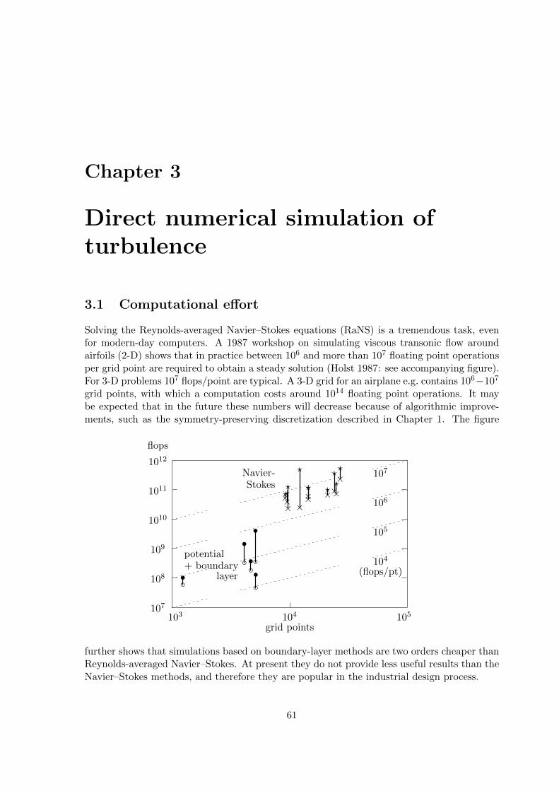
Chapter 3
Direct numerical simulation ofturbulence
3.1 Computational effort
Solving the Reynolds-averaged Navier–Stokes equations (RaNS) is a tremendous task, evenfor modern-day computers. A 1987 workshop on simulating viscous transonic flow aroundairfoils (2-D) shows that in practice between 106 and more than 107 floating point operationsper grid point are required to obtain a steady solution (Holst 1987: see accompanying figure).For 3-D problems 107 flops/point are typical. A 3-D grid for an airplane e.g. contains 106−107
grid points, with which a computation costs around 1014 floating point operations. It maybe expected that in the future these numbers will decrease because of algorithmic improve-ments, such as the symmetry-preserving discretization described in Chapter 1. The figure
103 104 105107
108
109
1010
1011
1012
grid points
flops
Navier-Stokes
×
?×?
×
?
×?×?
×
?
×? ×?×?
×?
potential+ boundary
layer•
•
•
•
•
104
105
106
107
(flops/pt)
further shows that simulations based on boundary-layer methods are two orders cheaper thanReynolds-averaged Navier–Stokes. At present they do not provide less useful results than theNavier–Stokes methods, and therefore they are popular in the industrial design process.
61
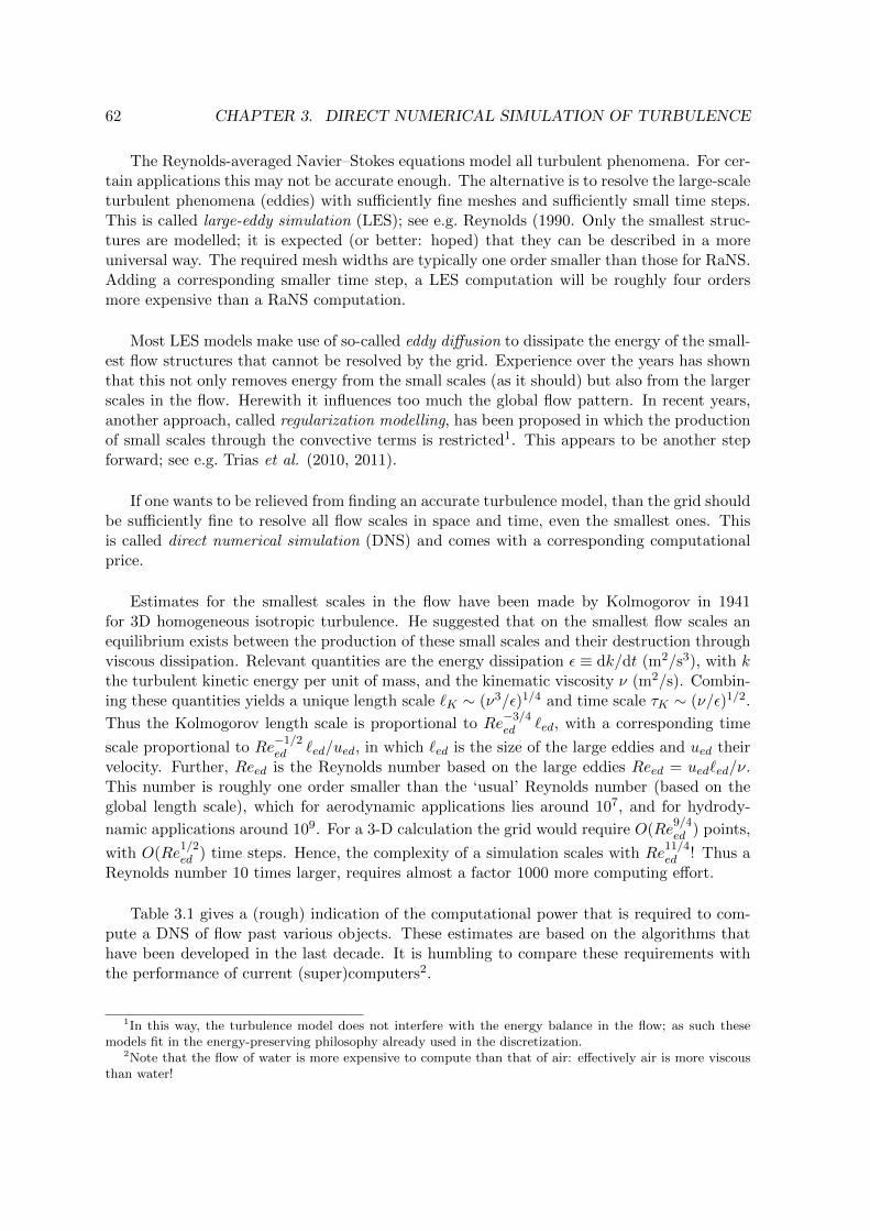
62 CHAPTER 3. DIRECT NUMERICAL SIMULATION OF TURBULENCE
The Reynolds-averaged Navier–Stokes equations model all turbulent phenomena. For cer-tain applications this may not be accurate enough. The alternative is to resolve the large-scaleturbulent phenomena (eddies) with sufficiently fine meshes and sufficiently small time steps.This is called large-eddy simulation (LES); see e.g. Reynolds (1990. Only the smallest struc-tures are modelled; it is expected (or better: hoped) that they can be described in a moreuniversal way. The required mesh widths are typically one order smaller than those for RaNS.Adding a corresponding smaller time step, a LES computation will be roughly four ordersmore expensive than a RaNS computation.
Most LES models make use of so-called eddy diffusion to dissipate the energy of the small-est flow structures that cannot be resolved by the grid. Experience over the years has shownthat this not only removes energy from the small scales (as it should) but also from the largerscales in the flow. Herewith it influences too much the global flow pattern. In recent years,another approach, called regularization modelling, has been proposed in which the productionof small scales through the convective terms is restricted1. This appears to be another stepforward; see e.g. Trias et al. (2010, 2011).
If one wants to be relieved from finding an accurate turbulence model, than the grid shouldbe sufficiently fine to resolve all flow scales in space and time, even the smallest ones. Thisis called direct numerical simulation (DNS) and comes with a corresponding computationalprice.
Estimates for the smallest scales in the flow have been made by Kolmogorov in 1941for 3D homogeneous isotropic turbulence. He suggested that on the smallest flow scales anequilibrium exists between the production of these small scales and their destruction throughviscous dissipation. Relevant quantities are the energy dissipation ε ≡ dk/dt (m2/s3), with kthe turbulent kinetic energy per unit of mass, and the kinematic viscosity ν (m2/s). Combin-ing these quantities yields a unique length scale `K ∼ (ν3/ε)1/4 and time scale τK ∼ (ν/ε)1/2.
Thus the Kolmogorov length scale is proportional to Re−3/4ed `ed, with a corresponding time
scale proportional to Re−1/2ed `ed/ued, in which `ed is the size of the large eddies and ued their
velocity. Further, Reed is the Reynolds number based on the large eddies Reed = ued`ed/ν.This number is roughly one order smaller than the ‘usual’ Reynolds number (based on theglobal length scale), which for aerodynamic applications lies around 107, and for hydrody-
namic applications around 109. For a 3-D calculation the grid would require O(Re9/4ed ) points,
with O(Re1/2ed ) time steps. Hence, the complexity of a simulation scales with Re
11/4ed ! Thus a
Reynolds number 10 times larger, requires almost a factor 1000 more computing effort.
Table 3.1 gives a (rough) indication of the computational power that is required to com-pute a DNS of flow past various objects. These estimates are based on the algorithms thathave been developed in the last decade. It is humbling to compare these requirements withthe performance of current (super)computers2.
1In this way, the turbulence model does not interfere with the energy balance in the flow; as such thesemodels fit in the energy-preserving philosophy already used in the discretization.
2Note that the flow of water is more expensive to compute than that of air: effectively air is more viscousthan water!

3.1. COMPUTATIONAL EFFORT 63
The Dutch national supercomputer that was installed in 2000 aimed at an effective per-formance around 100 Gigaflop/s (peak 1 Teraflop/s)3 Starting from here, about five orders ofmagnitude have to be bridged to perform a DNS of a turbulent flow at Re = 107. Assumingthat both computer hardware and computational algorithms will continue to progress at therate that they have developed during the past three decades – both have become one and ahalf order of magnitude faster per decade – within two decades the lacking five orders of mag-nitude could be bridged. For this estimate to come true, computers need to become about athousand times faster and must be supplied with one thousand times as much memory withinthe next two decades. Within that span of time the numerical algorithms for DNS need tobecome three orders of magnitude faster, need to run efficiently at the fastest available ma-chines, and need to use three orders of magnitude less memory than today’s algorithms dorequire.
medium speed Reynolds grid performancepoints (2 week run)
cyclist (tourist) air 20 km/h 1 · 105
golf ball (pro) air 250 km/h 2 · 105 109 1011.5 flop/sspeed skater (pro) air 45 km/h 5 · 105
swimmer (pro) water 5 km/h 3 · 106 1011 1014 flop/scar air 80 km/h 5 · 106
shark water 20 km/h 2 · 107 1013 1016.5 flop/sairplane air 900 km/h 3 · 107
ship water 20 km/h up to 109 1017 1021 flop/s
Table 3.1: Overview of (estimated) required computational resources (CPU performance) forDNS at Reynolds numbers in the range 105 − 109 (2010 algorithms).
In fact, the ASCI project in the USA, initiated in the mid 1990-ies, strived for this type ofperformance improvement. In 1999 already three computers existed where the 1 Teraflop/slimit has been achieved. The Supercomputer TOP500 of November 1999 was led by the prod-ucts of the ASCI project: on top of the list Intel’s ASCI Red with 2.4 Teraflop/s, followedby IBM’s Blue Pacific with 2.1 Teraflop/s and SGI’s Blue Mountain with 1.6 Teraflop/s.However, the type of application for which these processor speeds are achieved, the so-calledLinpack benchmark, is not fully representative for CFD. Linpack is very cache-friendly, i.e.once data have arrived in cache the algorithm makes frequent of use of them before they arereplaced by fresh data. In CFD algorithms the communication with main memory is muchmore frequent, and a factor of three (or more) is easily lost compared to Linpack performance.Thus, for CFD simulations computers with high access rates of memory (high bandwidth/lowlatency), such as vector computers where up 30-50% of peak performance can be achievedin practice, are very much in favour over commodity processors like Intel’s Xeon or AMD’sOpteron. On the latter machines only around 5% of peak performance can be achieved forCFD algorithms.
The TOP500 list has been dominated by (North-American) massively parallel cache-based(scalar) computers, under a constant challenge of (Japanese) computers based on vector ar-
3Giga= 109, Tera= 1012, Peta= 1015, Exa= 1018, Zetta= 1021, Yotta= 1024.

64 CHAPTER 3. DIRECT NUMERICAL SIMULATION OF TURBULENCE
Figure 3.1: Development of computer performance as illustrated by the Top500 list: top entry,#500 and the sum of all entries (Meuer and Gietl 2012).
chitecture; Figure 3.1 shows the developments between 1993 and 2012. E.g. for about threeyears, 2002-2004, the fastest computer was the Japanese NEC Earth Simulator, based on vec-tor processors, where 12 Teraflop/s sustained(!) performance could be achieved on codes forclimate modelling (36 Teraflop/s on Linpack). In June 2009, when the TOP500 was headedby several Intel, IBM and AMD based clusters, the two toppositions broke the Petaflop/s (=1000 Teraflop/s) barrier. Since then, the progress in cluster performance has continued. InJune 2012 the topposition, an IBM Blue Gene/Q, reached over 16 Petaflop/s on a clusterwith 1.6 million(!) cores. Plans are being made to attack the Exaflop/s barrier (1018 flop/s),hopefully to be reached in 2019 (Meuer and Gietl 2012).
Thus, the progress in computer hardware remains impressive. Together with the equallyimpressive progress in numerical algorithms, DNS computations at full-scale Reynolds num-bers glimmer at the horizon.
3.2 Navier–Stokes: higher-order space discretization
It will be clear that DNS requires the utmost of computers and algorithms. Therefore muchresearch is going on in improving the efficiency of algorithms. At RUG we have concen-trated on higher-order discretization methods along the lines presented in Section 1.5. Wewill apply the above ideas now to construct a higher-order discretization of the Navier–Stokesequations on the staggered grid as discussed above. In the described second-order methodthe x-momentum equation is applied to a control volume as shown in Figure 3.2 (left). Wenote that the vertical velocity is defined in the corner points of this volume.
The control volume now is combined with a larger one: for the convection-diffusion equa-tion above we chose a two-times larger volume, but here we will use a three-times largervolume as indicated in Figure 3.2 (right). The latter choice is the smallest volume for whichthe corners coincide with positions of the vertical velocity. The coinciding of corners with ver-

3.2. NAVIER–STOKES: HIGHER-ORDER SPACE DISCRETIZATION 65
Figure 3.2: The left picture shows a control volume for the conservation of the horizontalcomponent of the momentum field (in two spatial dimensions). The right picture shows athree-times larger control volume that is applied to eliminate the leading term of the truncationerror. The arrows denote the components of the discrete velocity that are used to discretizethe application of the conservation law to the control volume.
tical velocities implies that one discretization method can be used for the spatial integration ofthe momentum equation over both the original control volumes and the larger volumes. Twotimes larger control volumes, for instance, have corners that do not coincide with positionsof the vertical velocity, and thus do require additional high-order interpolations (e.g. for thecross terms in the convective flux). This interpolation unavoidably introduces some diffusionin the discretization, which does interfere with the real diffusion as we have experienced intest calculations. For DNS this is an unacceptable situation.
As in the convection-diffusion example above, near the boundaries we simply follow thesecond-order approach to avoid problems with control volumes that do not fit in the domain.
We update the velocity by integrating the momentum equations over one time step and bycorrecting the result by adding the pressure gradient in such a way that the mass is conservedin control volumes centred on the pressures. Obviously, we can also apply the balance ofmass to three times larger control volumes and use these control volumes to eliminate theleading term in the truncation error. Thus, a fourth-order-accurate spatial discretization canbe derived for the continuity equation. Since the ‘div’ and ‘grad’ operator analytically areeach other’s transpose (apart from a minus-sign; see Section 2.3), the discretization of thedivergence immediately implies the discretization of the gradient. Subsequently, the discreteLaplacian (= div grad) appearing in the pressure Poisson equation is implied. More elabo-rated details can be found in Verstappen and Veldman (2003).
The discrete Poisson equation for the pressure is solved by means of the conjugate gradientmethod with modified incomplete Choleski preconditioning according to Gustafson (1978).The MICCG code is fully vectorized by an explicit reordering of the unknowns along diagonalsof grid planes parallel to the symmetry plane of the cavity. The implementation of thepreconditioned iterative method is optimized as proposed by Eisenstat (1981). The initialguess for the iteration is obtained by extrapolation of the pressure from previous time levels.

66 CHAPTER 3. DIRECT NUMERICAL SIMULATION OF TURBULENCE
2nd- vs. 4th-order discretization
As an example of the progress made, we present a comparison between a second-order ap-proach and our fourth-order approach for flow in a 3D driven cavity at Re = 10, 000. Exper-imental results are available for comparison (Prasad and Koseff 1989). We show the verticalvelocity along the central axis of the cavity as obtained from a second-order calculation on a100× 100× 100 grid, a fourth-order calculation on a 50× 50× 50 grid and the experimentalresults. The overall error in an instantaneously measured velocity is about ± 0.6% of themaximum velocity. The stretching in the latter grid is moderate: the grid spacing is expo-nentially stretched away from the wall, and the largest mesh width is approximately seventimes wider than the smallest.
Figure 3.3: Lower-order and higher-order computation vs. experiment of tur-bulent flow in a 3D driven cavity atRe = 10, 000. Shown is the normal ve-locity along the central axes of the sym-metry plane.
In this example the fourth-order results are clearly superior to the second-order results,whereas the computational effort is about twenty times less. Indeed, the CPU-time per gridpoint and time step of both methods is comparable, a 503 grid has 8 times less grid points thana 1003 grid, it allows for a twice as large a time step (note that the time step is restricted bythe CFL-condition), and the number of iterations needed to solve the pressure correction fromthe Poisson equation is somewhat less for a 503 grid than for a 1003 grid: 8× 2× 1.25 = 20.Essential to this success is the way in which the discretization of the convective terms copeswith the stretching of the computational grid.
3.3 Refined time integration
In these lecture notes, mostly the explicit Forward-Euler time-integration method has beenused; not because it is the most efficient method, but it suits didactical purposes best. Runge–Kutta methods and multi-step methods (like Adams–Bashforth) – to stay within the explicitmethods – provide more efficiency. In this section we will discuss a refinement of the latter,which is better suited for (turbulent) flow simulations at large Reynolds numbers (Verstappenand Veldman 1998, 2003).
In Section 1.8 it was concluded that the diffusive stability limit is most restrictive whenthe cell-Peclet number P ≡ uh/ν < 2, but for P > 2 the convective limit dominates. Close toa solid wall the flow is laminar, with low velocities due to the (no-slip) boundary condition.Here, in wall-normal direction we have locally P < 2 and the diffusive limit is the most re-strictive. Further away from the wall the flow is turbulent and Kolmogorov’s estimates apply.

3.3. REFINED TIME INTEGRATION 67
For a grid size proportional to the Kolmogorov length scale `K ∝ ν3/4, the cell-Peclet numberscales with ν−1/4 and is likely to be > 2 (which should not be too bad as the resolution isOK). The (mathematical) convective stability limit becomes δtconv ∝ ν3/4, much less thanthe (physical) Kolmogorov time scale τK ∝ ν1/2. Thus, in the bulk of the flow domain theconvective stability limit is our main concern. Therefore, below we will present a simpleadaptation of the Adams–Bashforth method which is tuned to this situation and enhances itsefficiency by a factor of two.
Hereto we consider a family of explicit second-order one-leg methods, which will be dis-cussed with aid of the test problem u′ = f(u). For this problem the one-leg family reads
(α+ 12)u(n+1) − 2αu(n) + (α− 1
2)u(n−1) = δtf(
(1 + α)u(n) − αu(n−1)). (3.1)
This discretization is second-order accurate for all α 6= −13 , and third-order accurate when
α = −13 . Its error constant is given by C3 = 1
6(1 + 3α). The ‘one’ in one-leg refers to thefact that these methods evaluate the right-hand side f at one point only. For more details onone-leg methods the reader is referred, for instance, to Hairer (1991).
Taking α = 12 , a one-leg method is created which is the twin of Adams–Bashforth. Accord-
ing to Adams–Bashforth we ought to take 32f(u(n))− 1
2f(u(n−1)) instead of f(32u
(n)− 12u
(n−1)).One- and two-leg methods are identical when f is linear with time-independent coefficients,and then they have the same region of linear stability. They differ when the right-hand sidef is non-linear or explicitly time-dependent. For instance, in the ‘simple’ situation wheref(u) = λ(t) with λ(t) < 0 (i.e. u does not enter the right-hand side), the solution u(n+1) of(3.1), i.e.
u(n+1) = u(n) + δt λ(32 tn −
12 tn−1),
is smaller than u(n) (for any time step) as it should be. On the other hand, the solutionobtained with the associated multi-step method given by
u(n+1) = u(n) + δt 32λ(tn)− 1
2λ(tn−1)
does not satisfy the inequality u(n+1) < u(n) unconditionally (it depends on the variation of λwith time). In addition, it is emphasized in Nevanlinna (1978) that (some) one-leg methodsare more reliable than their corresponding multi-step methods when used with variable timesteps.
For α = 0 the leapfrog method is obtained. This method cannot be used to integrate adiffusive flux in time, since it is not stable: the linear stability region of leapfrog consists ofall purely imaginary numbers with modulus smaller than or equal to one.
Our aim is to determine α such that the corresponding method allows for the largesttime step, or stated otherwise, possesses the largest region of convective stability. Figure 3.4(left) shows the stability domain of the one-leg method for α = 0.05 and α = 0.5 (Adams–Bashforth). The stability domain is pressed against the imaginary axis when α goes to zero.In the limit α = 0 the stability domain is equal to the interval [−i, i]. Above we concludedthat convective stability puts the most severe restriction on the time step. Thus, we look forstability domains which include eigenvalues λ = x+ iy, where the real part x is negative and

68 CHAPTER 3. DIRECT NUMERICAL SIMULATION OF TURBULENCE
Figure 3.4: The left picture shows the stability domain of the one-leg method (3.1) for α = 0.05and α = 0.5. The right picture shows a blow up of the stability domains near the positiveimaginary axis.
the absolute value of the imaginary part y is much larger than the absolute value of the realpart. Here, ‘much’ can range from one to two orders of magnitude. For a DNS of a flow in adriven cavity at Re = 104 with a grid size δx = 10−2, and a maximum velocity Umax = 1, forexample, |x| : |y| is of the order of 1 : 100.
Under these conditions, the one-leg method with α = 0.05 outperforms Adams–Bashforth.Figure 3.4 (right) shows a blow up of the stability domains of both methods near the positiveimaginary axis. The points denoted by A and B lie on the line |x| : |y| = 1 : 20. The pointA lies close to the boundary of the stability domain for α = 0.05; B lies near the boundaryof the stability domain for α = 0.5. A lies approximately two times as far from the originas B. Thus, the time step of the one-leg method with α = 0.05 can be enlarged by a factorof two compared to Adams–Bashforth. For |x| : |y| = 1 : 10 this factor is about 1.5; for|x| : |y| = 1 : 100 it is approximately 2.5. We have carried out a number of numerical testcalculations of the (2D) flow in a driven cavity at Re = 103 − 105. The results demonstratethat the one-leg method with α = 0.05 requires indeed about two times less computationaleffort than the Adams–Bashforth method, whereas the accuracy is just as good.
3.4 Examples of turbulent-flow simulation
Both the algorithmic improvements and the improvements in computer performance haveopened the door to solve the Navier-Stokes equations numerically for Reynolds numbers inthe range 104 − 105 without using any turbulence model. Results in this range will first beshown in comparison with LES concerning the flow past a long, square cylinder at Re =22,000 (Section 3.4.1). Thereafter, in Section 3.4.2 a comparison is made between DNS andRaNS for a flow past an array of cubes. Finally (Section 3.4.3), results for a channel floware presented for which experimental results and early DNS computations are available. Formore details see Verstappen and Veldman (1996, 1997, 1998).
3.4.1 Flow past a square cylinder at Re = 22,000
The comparison with LES concerns the flow past a long, square cylinder at Re = 22,000 (atzero angle of attack). We assume that the flow is periodical in the spanwise direction. The

3.4. EXAMPLES OF TURBULENT-FLOW SIMULATION 69
spanwise boundaries are taken four diameters apart. We prescribe laminar inflow at six and ahalf diameters upstream of the cylinder. Experiments by Lyn et al. (1995) indicate a turbu-lence level (i.e. the ratio between the fluctuating and the mean velocity) of about 2% at fourand a half diameters upstream from the cylinder. The lateral boundaries are taken 14 diame-ters apart. The outflow boundary is positioned at 20 diameters past the cylinder. In addition,in a buffer zone (of five diameters length) the Reynolds number is decreased from 22,000 to1,000 to suppress (non-physical) waves which are reflected by the artificial outflow boundary.The (artificial) outflow conditions read vnn = wnn = 0 and pn = constant, where the con-stant is determined such that the mass inflow equals the mass outflow (at each time-step); thisconstant is approximately zero. No-slip boundaries are imposed at the surface of the cylinder.
We have used a 280×210×64 staggered grid to cover the computational domain. The firstgrid point is spaced 0·005 from the cylinder surface. The grid is stretched out away from thecylinder surface by means of a sinh function; the ratio of the largest to smallest grid size inthe streamwise direction is approximately 200. About 5% of the grid points are located in thebuffer zone. The discrete Poisson equation for the pressure is solved with a combination of aFast Fourier Transform method in the spanwise direction and a modified incomplete CholeskiConjugate-Gradient method in the resulting spectral space.
Figure 3.5: Snapshot of the flowpast a rectangular cylinder atRe=22,000. The visualisationhas been done with the spot-noisemethod (De Leeuw 1997).
The start-up of the flow plus three shedding cycles have been computed on 16 nodes of aCRAY J932. We compute averages over three shedding cycles by sampling the flow at eachtime step. Velocities are also averaged over the top and bottom halves. All quantities arenormalized by the cylinder width and the inflow velocity.
Simulation ExperimentsLyn et al. (1995) Lee (1975) Vickery (1966)
Mean Strouhal number 0·133 0·133± 0·003 − −Mean drag coefficient Cd 2·09 2·1 2·05 2·05Mean lift coefficient Cl 0·005 − − −Rms fluctuation of Cd 0·178 − 0·16− 0·23 −Rms fluctuation of Cl 1·45 − − 0·68− 1·32
Table 3.2: Comparison with experiment: bulk quantities

70 CHAPTER 3. DIRECT NUMERICAL SIMULATION OF TURBULENCE
Table 3.2 shows the mean Strouhal number, the mean drag coefficient Cd, the mean liftcoefficient Cl and the root-mean-square fluctuations of Cd and Cl. Here, it may be noted thatthe mean lift coefficient has not been measured; it should be zero by symmetry. All computedbulk quantities fall within the range set by the experiments, except for the root-mean-squareof the fluctuations of the lift coefficient Cl which is slightly overestimated. Figure 3.6 showsa comparison of mean streamwise velocities with experimental data at four locations past thecylinder. The agreement between the experimental data and the numerical data is good.
Figure 3.6: Flow past a square cylinder at Re=22000: a comparison of mean velocities ofthe fourth-order simulation with experimental results. The experimental data is taken fromERCOFTAC Database Case 43; see also Lyn et al. (1995). Shown is the mean streamwisevelocity. The continuous lines correspond to the simulation; the experimental data is depictedby the dots.
The flow past a square cylinder at Re = 22,000 (at zero angle of attack) has served asa test case at two LES workshops. The results submitted to the workshops can be foundin Rodi (1997) and Voke (1997). The results show a great variation in the predictions, andit was concluded that this flow forms a major challenge to current LES techniques; no onehas found the definite solution, yet. There is no doubt that the definite solution has to becomputed by means of an accurate, cost-effective numerical method. In Figure 3.7, we haveplotted the drag coefficients of almost all the submissions versus the numerical method thathas been applied. Here, we have left out a few, namely those that had serious failings (a toolarge lift coefficient, or a shedding frequency that differed significantly from the experiments).
There are of course many factors that (can) affect the prediction of the drag coefficient:the subgrid scale model, the value of parameters in the model, the grid resolution, the nu-merical approach, the treatment of the walls, etc. Unfortunately, these factors varied duringthe workshops, and consequently it is difficult to trace the source of the errors in the resultsof the simulations.
As can be seen in Figure 3.7, large-eddy simulations with a QUICK or a third-order up-wind (U3) discretization predict a drag force which is too large. The U3-approach that comesclosest to the experimental data uses approximately five times the number of grid points ofeach of the other QUICK/U3-methods. Although we cannot draw firm conclusions, for the

3.4. EXAMPLES OF TURBULENT-FLOW SIMULATION 71
Figure 3.7: Flow past a square cylinder at Re=22,000: the mean drag coefficient versus thediscretization of the convective terms of the Navier–Stokes equations. Here, U stands forupwind, and C for a central discretization. The number denotes the order of the method: C2,for example, represents a second-order central discretization. The experimental results of Lynet al. (1995), Lee (1975) and Vickery (1966) fall within the shaded area. The results of thelarge-eddy simulations are taken from Rodi (1997) and Voke (1997).
reason mentioned above, it is most likely that the artificial diffusion added by QUICK/U3contaminates the results.
The performance of subgrid models is difficult to judge since modelling errors and nu-merical errors interact; see also Vreman et al. (1994). To separate these errors, a numberof subgrid models need to be considered within the same numerical approach. We feel thatsymmetry-preserving methods provide a good basis for evaluating turbulence models, sincethey are accurate on non-uniform grids and the character of the numerical error is well-defined:the error in the convective term is convective; the error in the diffusive term is diffusive.
3.4.2 Surface mounted cubes
Next we show an example of a turbulent flow that has served as a test case for turbulencemodelling at the 6th ERCOFTAC/IAHR/COST Workshop on Refined Flow Modelling whichwas held at Delft University of Technology in June 1997 (Hanjalic and Obi 1997). The prob-lem considered is the fully developed flow in a channel where an array of 25 × 10 cubes isplaced regularly at the bottom. The Reynolds number based on the height of the channeland the bulk velocity is 13,000. The channel is 3.4 times wider than a cube. The pitch of thecubes is four cube lengths in both the streamwise and the spanwise direction.
Meinders et al. (1998) have measured this complex turbulent flow. Their flow measure-ments around the 18th row from the inlet showed that the influence of the in- and outletcan be neglected there. Hence, the computational domain for a numerical simulation can beconfined to a sub-channel unit of dimension 4h× 3.4h× 4h (where h denotes the height of acube) with periodic boundary conditions in both the streamwise and the spanwise directions.Figure 3.8 displays the sub-channel unit.
We have applied the fourth-order, symmetry-preserving method that is outlined in Sec-tion 3.2 to compute mean velocity profiles and Reynolds stresses at various locations in the

72 CHAPTER 3. DIRECT NUMERICAL SIMULATION OF TURBULENCE
Figure 3.8: Top- and side-view of a sub-channel unit. An instantaneous flow field at two planesthrough the centre of the cubes is shown, as obtained from the 1003 DNS. In both pictures theflow is directed from left to right. It may be noted that large structures of recirculating flowbehind the obstacles are not present in any of the snapshots of this flow. These regions canonly be observed if the flow is averaged over a long period in time.
sub-channel (Verstappen and Van de Velde, 2006). To this end, the sub-channel is covered bya 1003 grid. The first mesh point is spaced 0·006 to a wall. A cube is represented by 40 gridpoints in each direction. The grid is slightly stretched: the largest grid size is approximatelythree times the smallest. No-slip boundaries are imposed at the surfaces of the cubical ob-stacles and also on the walls of the channel.
The entire computation (including start-up and sampling time) took about 100 hours onone vector-processor of a CRAY C90. Mean velocity profiles as well as Reynolds stresses atvarious locations in the channel have been computed. The sampling of data for the computa-tion of the first- and second-order statistics of the flow started after a transitional period of100 (non-dimensional) time units. The time-averages were computed over 200 time units andover the two symmetrical halves of the sub-channel unit. Samples were taken at each timestep.
Figure 3.9 shows a comparison of the first- and second-order statistics4 of the 1003 simu-lation with the experimental data of Meinders et al. (1997) in the symmetry plane parallel tothe streamwise direction that bisects a cube. The agreement between the experimental dataand the numerical data is excellent.
In order to challenge RaNS computations, we have also performed a simulation at a 603
grid. On this grid, a cube is represented by 30 grid points in each direction. The first gridpoint of the 603 grid lies approximately twice as far from the wall than the first grid pointof the 1003 grid. The coarse grid simulation takes about one tenth of the CPU-time of the
4Because of the seemingly chaotic behaviour of turbulent flow, it makes little sense to compare snapshotsin time as in Figure 3.8 directly. Instead, one compares time averages and fluctuations around the mean as inFigure 3.9.

3.4. EXAMPLES OF TURBULENT-FLOW SIMULATION 73
Figure 3.9: Comparison of numerical results (continuous lines) with experiment (dots) forflow past an array of cubes. The left picture shows the mean streamwise velocity u, whereasthe right picture shows the fluctuating streamwise velocity u′u′.
fine grid simulation, among other things because the time step can be increased by a factorof about two.
There were four groups who presented results of their RaNS computations of the flow inthe channel with surface-mounted cubes at the workshop (Hanjalic and Obi 1997). Here, werestrict ourselves to the RaNS computation (of Dr. S. Jansson from the Department of FluidMechanics of Vattenfall Entvecklung AB in Sweden) that agreed the best with the availableexperimental data. It may be noted that there were no results of large-eddy simulationssubmitted to this workshop, nor have there been any reported elsewhere.
The best RaNS result was based on a second-order, cell-centered, finite-volume method.The QUICK scheme was used for the velocities and the turbulent quantities were integratedby means of a second-order accurate scheme with a Van Leer limiter. Periodic boundaryconditions were applied in the streamwise direction; the period was taken equal to four cubelengths. Symmetry conditions were applied in the spanwise directions. The spanwise bound-aries were taken two cube lengths apart. Dirichlet conditions were applied at the solid walls,except for the dissipation rate ε: the normal derivative of ε was put to zero at solid walls.The turbulence model consisted of a two-layer eddy-viscosity combined with a standard k− εmodel. The transport equation for the dissipation rate ε was not solved in near-wall regions,but instead it was computed explicitly from a predicted length scale. This RaNS computationwas performed on a stretched, orthogonal grid of 67 × 72 × 57 points in the streamwise, thenormal and the spanwise direction, respectively. Except for the spanwise direction, the gridspacing of this RaNS computation is slightly finer than that of our 603 simulation. In thespanwise direction, the average resolution of the RANS computation is about two times finerthan the average resolution of the 603 grid, due to the fact that the RaNS computation usessymmetry conditions and therefore can restrict its spanwise computational domain to twocube lengths, while in our simulation periodic boundary conditions have been applied in thespanwise direction with a period of four cube lengths.
Mean streamwise velocities are compared in Figure 3.10. On a corresponding grid, themean velocities computed from the Reynolds averaged Navier–Stokes equations agree less

74 CHAPTER 3. DIRECT NUMERICAL SIMULATION OF TURBULENCE
Figure 3.10: Comparison of the mean streamwise velocity at half cube height. The flow comesfrom below; the horizontal corresponds to the spanwise direction. The dashed vertical linesare lines of symmetry; their distance is two cube lengths. The lowermost profiles are locatedat 0.3 cube lengths before the front of the cube, the middlemost profiles at 0.3 cube lengthsafter the front an the uppermost profiles at one cube length after the middlemost. The velocityscale is shown for the uppermost profiles only. The experimental data is taken from Meinders(1997); the RaNS data is taken from Hanjalic and Obi (1997).
with the experimental data than the results of the symmetry-preserving simulation. Thevelocity profiles of the RaNS computation are much too smooth. In addition, the maximaof the velocities are located in the symmetry-plane between two cubes, which is in distinctdisagreement with the experimental data.
Finally, it may be observed that the convergence of the symmetry-preserving simulationupon grid refinement is plain: the results on the 1003 grid are closer to the measurementsthan those of the 603 grid.
3.4.3 Channel flow
To further illustrate the accuracy of the symmetry-preserving discretization, consider a turbu-lent channel flow at a Reynolds number of Re=5,600. A large number of numerical results aswell as experimental data is available for comparison. Figure 3.11 (left) shows a comparisonof the mean velocity profile as obtained from the 4th-order symmetry-preserving simulationwith those of other direct numerical simulations. The grids used by the DNS’s that we com-pare with have typically about 1283 grid points, that is 16 times more grid points than ourgrid has. Nevertheless, the agreement is excellent.

3.4. EXAMPLES OF TURBULENT-FLOW SIMULATION 75
Figure 3.11: Comparison of the mean streamwise velocity u+ (left) and its root-mean-square(right) as function of the wall normal coordinate y+.
The root-mean-square of the fluctuating streamwise velocity urms near the wall (0 < y+ <40) is presented in Figure 3.11 (right). The results show that the urms predicted by the 4th-order simulation fits the experiment data of Kreplin and Eckelmann (1979) nicely. This holdsfor very coarse grids too, as can be inferred from the results computed with the 4th-ordersymmetry-preserving scheme with only 32 grid points in the wall-normal direction. It is in-teresting to compare the ratio between ‘our’ 32 or 64 grid points in wall-normal direction andthe 128 grid points used in the reference computations (Kim et al. 1987, Kuroda el al. 1995,Gilbert and Kleiser 1991). This ratio (a factor two to four) compares quite well with the‘predicted’ possible increase in grid size (a factor of three) as found in the one-dimensionaltest case described in Section 1.7.
Figure 3.12: Convergence of the skin-friction coefficient upon grid refinement, displayed as afunction of the fourth power of the cell size next to the wall.
This flow case has also been used to carry out a grid refinement study to show indeed4th-order convergence behaviour. The skin-friction coefficient Cf has been monitored as ob-tained from simulations on five different grids, denoted A – E. Their spacings differ only inthe direction normal to the wall, with 128 (A), 96 (B), 64 (C), 56 (D) and 48 (E) points,

76 CHAPTER 3. DIRECT NUMERICAL SIMULATION OF TURBULENCE
respectively. The first (counted from the wall) grid line varies between y+1 = 0.72 (grid A) and
y+1 = 1.9 (grid E). The refinement study, as indicated in Figure 3.12, clearly shows a 4th-order
behaviour on the non-uniform grid. The straight line in Figure 3.12 is approximately given byCf = 0.008364− 0.000004(y+
1 )4. The extrapolated value at the crossing with the vertical axisy+
1 = 0 lies in between the Cf = 0.00818 reported by Kim et al. (1987) and Dean’s correlationCf = 0.073Re−1/4 = 0.00844. Note that the extrapolation eliminates the (leading term ofthe) discretization error in the wall-normal direction, but not the other discretization errorsin space and time.
Figure 3.13: The root-mean-square velocity fluctuations normalized by the wall shear velocityas a function of the wall coordinate y+ on various grids for y+ ≤ 20 (left) and y+ ≤ 200(right).
The convergence of the fluctuating streamwise velocity near the wall (0 < y+ < 20) ispresented in Figure 3.13 (left). Here, we have added results obtained on three still coarsergrids (with 32, 24 and 16 points in the wall-normal direction, respectively), since the results onthe grids A–E fall almost on top of each other. The coarsest grid, with only 16 points to coverthe channel width is coarser than most of the grids used to perform a large-eddy simulation(LES) of this turbulent flow. Nevertheless, in the near wall region, the 64× 16× 32 solutionis not that far off the solution on finer grids. Further away from the wall, the turbulentfluctuations predicted on the coarse grids (32 points or less in vertical direction) become toohigh compared to the fine grid solutions, as is shown in Figure 3.13 (right).
3.5 References
S.C. Eisenstat (1981) Efficient implementation of a class of preconditioned Conjugate Gradient meth-ods, SIAM J. Sci. Stat. Comput. 2, 1–4.
N. Gilbert and L. Kleiser (1991) Turbulence model testing with the aid of direct numerical simulationresults. In: Proc. Turb. Shear Flows 8, paper 26-1.
I. Gustafson (1978) A class of first order factorization methods. BIT 18, 142–156.
E. Hairer and G. Wanner (1991) Solving Ordinary Differential Equations II. Berlin: Springer-Verlag.
K. Hanjalic and S. Obi (eds.) (1997) Proc. 6th ERCOFTAC/IAHR/COST Workshop on RefinedFlow Modeling, Vol. 3, Section Heat Transfer, Delft University of Technology, 38 pages.

3.5. REFERENCES 77
T.L. Holst (1987) Viscous transonic airfoil workshop compendium of results. AIAA paper 87–1460.
J. Kim, P. Moin and R. Moser (1987) Turbulence statistics in fully developed channel flow at lowReynolds number. J. Fluid Mech. 177, 133–166.
L. Kleiser and T.A. Zang (1991) Numerical simulation of transition in wall-bounded shear flows.Annu. Rev. Fluid Mech. 23, 495–537.
H.P. Kreplin and H. Eckelmann (1979) Behavior of the three fluctuating velocity components in thewall region of a turbulent channel flow. Phys. Fluids 22, 1233–1239.
A. Kuroda, N. Kasagi and M. Hirata (1995) Direct numerical simulation of turbulent plane Couette-Poiseuille flows: effect of mean shear rate on the near-wall turbulence structures. In: F. Durstet al. (eds.) Proc. Turb. Shear Flows 9. Berlin: Springer-Verlag, pp. 241–257.
B.E. Lee (1975) The effect of turbulence on the surface pressure field of square prisms. J. Fluid Mech.69, 263–282.
W. de Leeuw (1997) Presentation and Exploration of Flow Data. Ph.D. Thesis, Delft University ofTechnology, Delft, 107 pages.
D.A. Lyn, S. Einav, W. Rodi and J.H. Park (1995) A laser-Doppler-velocimetry study of emsemble-averaged characteristics of the turbulent near wake of a square cylinder. J. Fluid Mech. 304,285–316.
E.R. Meinders, T.H. van der Meer and K. Hanjalic (1998) Local convective heat transfer from anarray of wall-mounted cubes. Int. J. Heat Mass Transfer 41, 335–346.
H.W. Meuer and H. Gietl (2012) Supercomputers Prestige Objects or Crucial Tools for Science andIndustry?. University of Mannheim $ Prometeus GmbH (Germany), 21 pages.
O. Nevanlinna and W. Liniger (1978) Contractive methods for stiff differential equations; Part I. BIT18, 457–474.
A.K. Prasad and J.R. Koseff (1989) Reynolds number and end-wall effects on a lid-driven cavity flow.Phys. Fluids A, 1, 208–218.
W.C. Reynolds (1990) The potential and limitations of direct and large eddy simulations. In: J.L.Lumley (ed.) Whither Turbulence: Turbulence at the Crossroads. Springer Verlag, pp. 313–342.
W. Rodi, J.H. Ferziger, M. Breuer and M. Pourquie (1997) Status of Large Eddy Simulation: Resultsof a workshop. ASME J. Fluids Eng. 119, 248–262.
F.X. Trias and R.W.C.P. Verstappen (2011) On the construction of discrete filters for symmetry-preserving regularization models. Comp. Fluids 40, 139–148.
F.X. Trias, R.W.C.P. Verstappen, A. Gorobets, M. Soria and A. Oliva (2010) Parameter-free symmetry-preserving regularization modeling of a turbulent differentially heated cavity. Comp. Fluids 39,1815–1831.
R.W.C.P. Verstappen and R.M. van de Velde (2006) Symmetry-preserving discretisation of heattransfer in a complex turbulent flow. J. Eng. Math. 54, 299–318.
R.W.C.P. Verstappen and A.E.P. Veldman (1996) A fourth-order finite volume method for directnumerical simulation of turbulence at higher Reynolds numbers. In: J.-A. Desideri et al. (eds.)Computational Fluid Dynamics ’96 . John Wiley, pp. 1073–1079.
R.W.C.P. Verstappen and A.E.P. Veldman (1997) Direct numerical simulation of turbulence at lowercosts. J. Eng. Math. 32, 143–159.
R.W.C.P. Verstappen and A.E.P. Veldman (1998) Spectro-consistent discretization: a challenge toRANS and LES. J. Eng. Math. 34, 163–179.

78 CHAPTER 3. DIRECT NUMERICAL SIMULATION OF TURBULENCE
R.W.C.P. Verstappen and A.E.P. Veldman (2003) Symmetry-preserving discretization for turbulentflow. J. Comput. Phys. 187, 343–368.
B.J. Vickery (1966) Fluctuating lift and drag on a long square cylinder of square cross-section in asmooth and in a turbulent stream. J. Fluid Mech. 25, 481–494.
P.R. Voke (1997) Flow past a square cylinder: test case LES2. In: J.P. Chollet et al. (eds.), Directand Large Eddy Simulation II, pp. 355–373.
B. Vreman, B. Geurts and H. Kuerten (1994) Discretization error dominance over subgrid-termsin large eddy simulation of compressible shear layers in 2D. Comm. Num. Meth. Eng. 10,785–790.

Appendix A
Discretization, integration anditeration
In the appendix we will give a short review of numerical fundamentals concerning spacediscretization, time integration and iterative solution of (sparse) systems of equations.
A.1 Discretization in space
Space discretization methods are often divided in four approaches:
– finite-difference methods;– finite-volume methods;– finite-element methods; and– spectral methods.
This subdivision is not strict in the sense that combinations of the above approaches alsoappear, such as ‘control-volume finite elements’ or ‘spectral elements’. Also, a number ofdiscretization formulas can be derived along several of these approaches. Here, we will onlymake some remarks on the first two approaches. They make use of a computational grid,typically denoted by
Ωh = (ih1, jh2)|i = 0, 1, · · · , I; j = 0, 1, · · · , J,
where h1 and h2 are the respective mesh widths.
(i, j)
Γh
h2
h1 -
?
6
Ωh eee
ee e
e e
e e e
e e e
uu
u uu u
79

80 APPENDIX A. DISCRETIZATION, INTEGRATION AND ITERATION
Some notation: The discrete approximation of an unknown function φ is denoted by φh.The value of the grid function φh in the grid point (ih1, jh2) - or short (i, j) - is denotedby φij . The boundary of Ωh is denoted by Γh. Internal grid points are collected in Ω0
h, theboundary points with a Dirichlet (or Robin) condition are denoted by ΓDh , and ΓNh is the setof boundary points with a Neumann condition.
A.1.1 Finite-difference methods
In a finite-difference method derivatives are approximated by combining local Taylor seriessuch that the local truncation error becomes satisfactory in some sense, e.g. minimizedbetween all other combinations using the same neighbouring grid points. As an example,consider the i-th grid point with its two nearest neighbours, corresponding to Taylor series
φ(xi + h) = φi + hdφ
dx
∣∣∣∣xi
+h2
2
d2φ
dx2
∣∣∣∣xi
+O(h3). (A.1)
and
φ(xi − h) = φi − hdφ
dx
∣∣∣∣xi
+h2
2
d2φ
dx2
∣∣∣∣xi
−O(h3). (A.2)
Subtracting (A.1) and (A.2) we obtain an estimate for the first-order derivative
dφ
dx
∣∣∣∣xi
=φi+1 − φi−1
2h+O(h2). (A.3)
which possesses a second-order accurate truncation error (cf. the term O(h2)). This formulauses two points positioned symmetrically with respect to the central point. As an alternativeone of these neighbours can be combined with the central point, yielding a formula that isonly first-order accurate
dφ
dx
∣∣∣∣xi
=φi − φi−1
h+O(h).
As we will demonstrate in Chapter 1, minimization of the local truncation error maynot be the optimum criterion for selecting discretization formulas (see also the discussion inSection A.1.4).
A.1.2 Finite-volume methods
A finite-volume method starts with a physical conservation law expressing conservation ofsome quantity φ over a domain Ω with boundary Γ
∂
∂t
∫Ωφ dΩ = −
∫ΓF (φ) · ndΓ +
∫Ωf dΩ. (A.4)
The integral over Γ describes the nett outflow of the considered quantity (given by the flux-function F (φ)), whereas f represents a source term. When the flux-function is differentiable,Gauss’ divergence theorem can be applied∫
Ω
∂φ
∂tdΩ +
∫Ω
divF (φ) dΩ =
∫Ωf dΩ.

A.1. DISCRETIZATION IN SPACE 81
Since this holds for arbitrary small volumes Ω the conservation law can be written as a PDEin divergence form
∂φ
∂t+ divF (φ) = f. (A.5)
Note that the physical conservation law (A.4) requires less smoothness of the solution; more-over it induces the correct jump relations.
t tt
t
t
E
N
W
S
P
rr
rr e
n
w
s
Ω
Γ
In the finite-volume method the relation (A.4) isapplied to individual control volumes, surrounding thegrid points. We give a typical example of a finite-volume grid in the adjacent figure. The control vol-umes are indicated by dashed lines, which lie halfwaybetween the grid point P = (xi, yj) and its neighboursN , E, S and W .
The integrals appearing in (A.4) can be approximated by e.g. the midpoint rule as
h1h2∂
∂tφP = −h2 [F1(φ)|e − F1(φ)|w]− h1 [F2(φ)|n − F2(φ)|s] + h1h2fP ,
in which F1 and F2 are the components of the flux-function. After division by h1h2 thisformula can be reshaped as follows
d
dtφh = −Lhφh + f, (A.6)
but as we will see in Section 1.5 this scaling is not always desirable. The ‘curly’ ∂/∂t has beenreplaced by a ‘straight’ d/dt, since in the right-hand side no spatial derivatives appear any-more. In time direction no discretization has taken place yet; we call this semi-discretization.
A.1.3 Properties of difference operators
Irrespective of the followed discretization approach, ultimately a spatial differential operatoris approximated by a difference operator which acts on functions defined on the computationalgrid. Such a difference operator will be of the form
(Lhφ)ij =∑k,l
cklij φkl. (A.7)
Definition A.1.1 The operator Lh defined in (A.7) is called positive1when∑k,l
cklij = 0, (i, j) ∈ Ω0h ∪ ΓNh ; (A.8)
cklij ≤ 0, (i, j) ∈ Ω0h ∪ ΓNh , (k, l) 6= (i, j). (A.9)
1Condition (A.8) implies that a positive operator can also be written in the form (Lhφ)ij =∑kl6=ij c
klij (φkl−
φij), with all relevant cklij ≤ 0 according to (A.9).

82 APPENDIX A. DISCRETIZATION, INTEGRATION AND ITERATION
The above requirements need only hold in the interior Ω0 and on Neumann boundaries ΓN ;on a Dirichtlet boundary ΓD they are not applicable since only a central coefficient cijij ispresent there.
A positive operator satisfies a maximum principle, which gives smoothness to the solution:the above definition implies that the solution in a grid point is a convex combination of itsneighbours:
φij =∑
(k,l)6=(i,j)
−cklij
cijijφkl,
with all coefficients in the right-hand side non-negative and adding up to 1. A fortiori , whenthere is a direct link between adjacent grid points, the solution of Lhψh = 0 is non-oscillatory(‘no wiggles’).
Theorem A.1.2 (Maximum principle) Let Lh, as defined in Def. A.1.1, be a positive oper-ator and suppose Lhφh ≤ 0 in Ω0
h ∪ ΓNh . Suppose also that Lh satisfies a direct-neighbourcondition
cklij 6= 0, (k, l) ∈ (i± 1, j), (i, j ± 1), (i, j) ∈ Ω0 ∪ ΓN , (A.10)
then φh can only take its maxima on ΓDh (unless φh is constant).
Proof Suppose φh takes its maximum M in the grid point (i, j) ∈ Ω0h ∪ ΓNh . Suppose Lh is given by
(A.7). Then from ∑k,l
cklij φkl = (Lhφh)ij ≤ 0
we havecijij φij ≤ −
∑(k,l)6=(i,j)
cklij φkl.
As the coefficients in the right-hand side are all non-positive we obtain
cijij φij ≤ −∑
(k,l) 6=(i,j)
cklij maxk,l
φkl = cijij maxk,l
φkl = cijijM.
Because φij = M , everywhere the equality sign has to hold, from which we conclude that all neighbours
φkl for which cklij 6= 0 have to be equal to M too. Because of the direct-neighbour condition (A.10),
the stencils with centre in Ω0h ∪ ΓNh share some overlap, with which the theorem follows. 2
Remark When the direct-neighbour condition (A.10) holds, whereas all other neighbour co-efficients vanish, than the maximum principle also holds for local maxima.
Corollary Let Lh be a positive operator satisfying the direct-neighbour condition (A.10),and let Lhφ1 = f1 and Lhφ2 = f2 with f1 ≤ f2. Then φ1 ≤ φ2.
Proof Apply Th. A.1.2 to Lh(φ1 − φ2) = f1 − f2. 2
Because of this property, positive operators are also called monotone. There exists alink with the so-called M -matrices (see Def. A.2.9), which form an important subclass of themonotone matrices (for which A−1 ≥ 0).

A.1. DISCRETIZATION IN SPACE 83
Theorem A.1.3 When the Dirichlet part of the boundary is non-empty, then a positiveoperator gives rise to an M -matrix. When Lh also satisfies a direct-neighbour condition(A.10) then the matrix is irreducible.
Proof The sign requirement for an M -matrix follows immediately from the definition (A.9) of a
positive operator. Further, because of (A.8) the matrix is (weakly) diagonally dominant. In Dirichlet
boundary points the diagonal dominance is strict. Now a Gershgorin-type argument yields that all
eigenvalues lie in the right half plane. 2
Next to their monotonicity property, leading to smooth solutions as discussed above, M -matrices also possess pleasant iterative properties, e.g. Jacobi and Gauss-Seidel iteration con-verge (see Section A.2). Unfortunately, one has to pay a price for such favourable properties,as formulated in the following theorem.
Theorem A.1.4 (Order barrier) Positive (hence monotone) discretizations of a first-orderderivative can maximally be first-order accurate.
Proof For a uniform one-dimensional grid with grid size h.) Suppose in grid point i we have
dφ
dx
∣∣∣∣i
≡∑k
ckφi+k.
A Taylor expansion of the occurring φ-values results in
dφ
dx
∣∣∣∣i
≡∑k
ck
(φi + kh
dφ
dx
∣∣∣∣i
+ 12 (kh)2
d2φ
dx2
∣∣∣∣i
+O(h3)
). (A.11)
As this expression is meant to be a discrete approximation for the first-order derivative, consistencyrequires that the zero-th order term vanishes and that the first-order term is equal to dφ/dx. Theseconditions can be satisfied. But, to achieve second-order accuracy, the second-order term in (A.11)should also vanish (note that ck ∝ 1/h), i.e.∑
k
12 (hk)2ck = 0.
Alas, this is impossible when all neighbouring coefficients ck ≤ 0, as required for a positive operator. 2
For more information on monotone discretization methods we refer to e.g. Chapter 21 ofHirsch (1990).
A.1.4 Discretization error
The above differential operators are being used for approximating (partial) differential oper-ators. Suppose the differential equation is given by
Lφ = f,
and the difference approximation by
Lhφh = fh.

84 APPENDIX A. DISCRETIZATION, INTEGRATION AND ITERATION
In general, the exact solution of the PDE will not satisfy the difference approximation. Thedifference
τh ≡ Lhφ− fh = Lh(φ− φh) (A.12)
is called the local truncation error. When h → 0 implies that τh → 0, then the differenceapproximation is called consistent.
The difference φ− φh, between the exact solution and the discrete solution, is called theglobal discretization error. Both errors are related by
φ− φh = L−1h τh. (A.13)
We have convergence when the global discretization error vanishes upon grid refinement (i.e.when h → 0). Note that the right-hand side in (A.13) consists of a product of the inversedifference operator and the local truncation error, hence smallness of the latter does notnecessarily lead to an accurate discrete solution (cf. the discussion in Section 1.5).
A.2 Elementary iterative solution methods
After discretization and linearization of a partial differential equation often a linear systemAx = b has to be solved. In this section we will summarize a number of iterative stationaryone-step methods. These have the generic form
Qx(n+1) = (Q−A)x(n) + b, n = 0, 1, · · · , (A.14)
where Q is a non-singular matrix. By rewriting (A.14) we obtain
x(n+1) = Cx(n) +Q−1b, n = 0, 1, · · · , where C = I −Q−1A. (A.15)
The matrix C is called the iteration matrix.
Since the iteration error, i.e. the difference with the exact solution x, satisfies
x− x(n+1) = C(x− x(n)),
the iteration method (A.15) will converge if and only if Cn → 0. The growth of Cn is givenby
‖Cn‖ ∼ cnp−1|λ|n−(p−1), n→∞, (A.16)
where λ is the modulus of the largest eigenvalue of C, and p the order of the largest Jordanblock corresponding with eigenvalues of modulus λ. It easily follows that an iterative methodis convergent if and only if its spectral radius ρ(C) < 1. The behaviour of Cn can be veryirregular when defect eigenvalues are present (i.e. eigenvalues for which no eigenvector exists)which give rise to Jordan blocks.
A.2.1 Jacobi and JOR
Write the matrix A as A = D − L − U , in which D = diag(A), L a strict lower-triangularmatrix and U a strict upper-triangular matrix. A simple splitting of the matrix is obtainedby only leaving its diagonal in the left-hand side
Dx(n+1) = (D −A)x(n) + b,

A.2. ELEMENTARY ITERATIVE SOLUTION METHODS 85
which upon division by D becomes
x(n+1) = (I −D−1A)x(n) +D−1b. (A.17)
The iteration matrix of this process I −D−1A = D−1(L+ U) is called the Jacobi matrix.
When the iteration process behaves very regularly, it may pay off to extrapolate the stepx(n+1) − x(n) as
x(n+1) = x(n) + ω(x∗ − x(n)) = ωx∗ + (1− ω)x(n),
where x∗ is the value from (A.17). This idea is called relaxation, and ω is the relaxationfactor. Adding relaxation to the Jacobi method (A.17) gives
x(n+1) = [ω(I −D−1A) + (1− ω)I ] x(n) + ωD−1b (A.18a)
= (I − ωD−1A)x(n) + ωD−1b (A.18b)
= x(n) − ωD−1(Ax(n) − b). (A.18c)
From (A.18b) we conclude
1
ωDx(n+1) = (
1
ωD −A)x(n) + b,
which shows a splitting where D/ω is left on the diagonal in the left-hand side. This methodis called JOR: Jacobi with OverRelaxation (although often ω < 1, i.e. underrelaxation, givesbetter results). The components of x(n+1) can be computed independent of each other; themethod is perfectly vectorizable and parallelizable.
In formulation (A.18c) we recognize the residual Ax(n) − b. This shows that in simplewords the JOR method can be expressed as: “the new guess equals the old guess plus a factortimes the residual”. We will use this interpretation several times in these lecture notes.
Next let us investigate the convergence behaviour of JOR. We will restrict ourselves firstto the class of weakly diagonally dominant matrices, which include the M -matrices.
Theorem A.2.1 When the matrix A is irreducible and weakly diagonally dominant, i.e.
|aii| ≥∑j 6=i|aij | for all i, with strict inequality for at least one i,
then the Jacobi method converges.
Proof Young (1971), Th. 4-2.1. 2
Theorem A.2.2 When Jacobi converges, then also JOR with 0 < ω ≤ 1 converges.
Proof From (A.18a), the iteration matrix of JOR is given by ω(I−D−1A)+(1−ω)I. Its eigenvaluesµJOR are related the eigenvalues µJ of the Jacobi matrix by
µJOR = ω µJ + 1− ω = 1 + ω (µJ − 1).

86 APPENDIX A. DISCRETIZATION, INTEGRATION AND ITERATION
r1
aaaaaaaa
r rµJ
µJOR
+
ω|µJ − 1|
CCO
r
r
LLLLLLLLLL""
""r9
1√1+µ2I
µI
16
ρopt
Observe that this corresponds with inter(extra)polation between the points 1 and µJ in the complex
plane. The figure reveals that as soon as Jacobi converges, i.e. all Jacobi eigenvalues lie within the
unit circle, all eigenvalues for JOR with 0 < ω ≤ 1 also lie within the unit circle. This establishes the
proof. 2
The above proof reveals that the eigenvalues of the Jacobi matrix I −D−1A have to lieon the left side of the line <eµ = 1. Thus, for complex eigenvalues we have in general
Theorem A.2.3 The JOR method converges for sufficiently small ω(>0) if and only if thematrix D−1A is positive-stable (i.e. all eigenvalues of D−1A are located in the right halfplane).
In many cases the eigenvalues of the Jacobi matrix lie outside the unit circle, hence theJacobi method will no longer converge. Often the eigenvalues lie far up on the imaginaryaxis. Let the largest eigenvalue be given by µJ = iµI , with µI real. In the above figure weobserve that the JOR method converges for 0 < ω < ωJOR,max where ωJOR,max = 2
1+µ2I. The
optimum relaxation factor is given by
ωJOR,opt =1
1 + µ2I
, with spectral radius ρJOR,opt =µI√
1 + µ2I
. (A.19)
A.2.2 Gauss-Seidel and SOR
In the Gauss-Seidel method also the lower-triangular part of the matrix is kept in the left-handside, hence
(D − L)x(n+1) = Ux(n) + b.
Its relaxation version SOR (Successive OverRelaxation) reads
(1
ωD − L)x(n+1) =
[(
1
ω− 1)D + U
]x(n) + b,
with iteration matrixCω = (D − ωL)−1[(1− ω)D + ωU ]. (A.20)
For consistently ordered matrices (see Young, 1971) a relation exists between the eigen-values λ of Cω and the eigenvalues µJ of the Jacobi matrix. This relation reads
(λ+ ω − 1)2 = ω2µ2Jλ.
A special case is ω = 1, when this relation reduces to λ = µ2J . This implies that for consis-
tently ordered matrices Gauss-Seidel converges if and only if Jacobi converges. More precise,

A.2. ELEMENTARY ITERATIVE SOLUTION METHODS 87
for such matrices Gauss-Seidel converges/diverges twice as fast as Jacobi. As a corollary,Gauss-Seidel converges for consistently ordered M -matrices.
For a large class of matrices SOR can be made convergent, as shown in the next theorem.
Theorem A.2.4 Let A be a consistently ordered matrix. Then SOR converges for sufficientlysmall ω(>0) if and only if D−1A is positive-stable.
Proof Young (1971), Th. 6-4.2. 2
Figure A.1: Relation between spectral radius, relaxation factor and Jacobi eigenvalue µ =µR + iµI .
In Figure A.1 we show the spectral radius of the SOR matrix (A.20) for various choices ofthe determining Jacobi eigenvalues. We note that for a symmetric matrix A (for which theJacobi spectrum is real), SOR converges if and only if A is positive definite and 0 < ω < 2.The optimum relaxation factor is given by (see Young (1971) Th. 4-3.3 and 4-3.6)
ωSOR,opt =2
1 + (1− µ2R)1/2
, with ρSOR,opt = ωSOR,opt − 1.
When the Jacobi eigenvalues are complex, than the ω-interval for which convergence occursbecomes smaller. For purely imaginary Jacobi spectra, with extremal eigenvalues µJ = iµI ,it can be shown (Botta and Veldman 1982) that SOR converges if and only if
0 < ω < ωSOR,max with ωSOR,max =2
1 + µI.
Hence, when µI > 1 Gauss-Seidel no longer converges (in fact, Jacobi does neither). Theoptimum relaxation factor is given by
ωSOR,opt =2
1 + (1 + µ2I)
1/2, with ρSOR,opt = 1− ωSOR,opt. (A.21)
It follows that ωSOR,opt < 1, i.e. underrelaxation is desired (and for µI > 1 even necessary).

88 APPENDIX A. DISCRETIZATION, INTEGRATION AND ITERATION
A.2.3 Some definitions and theorems on eigenvalues
In this section we present some definitions and theorems on the location of matrix eigenvalues.
Lemma A.2.5 (Bendixson) Let A = R + i S be a general (complex) matrix, where 2R =A + A∗ is its symmetric part, and 2iS = A − A∗ its skew-symmetric part (hence R and Sare Hermitian2). Let ρm and ρM be the smallest and largest eigenvalues of R, respectively;similarly σm and σM w.r.t. S. Then the eigenvalues of A are located in a rectangle definedby the lower-left and upper-right corners (ρm, σm) and (ρM , σM ).
Proof (from Householder 1964, p. 79) Let x be a normed eigenvector (i.e. x∗x = 1) correspondingto an eigenvalue λ = a+ i b of A. Then
a+ i b = λ = λx∗x = x∗Ax = x∗Rx+ i x∗Sx,
hence a = x∗Rx and b = x∗Sx. Since both R and S are Hermitian matrices their eigenvalues are realand one has
ρm ≤ x∗Rx ≤ ρM for any x;
a similar relation holds for S. Now the theorem follows. 2
Definition A.2.6 (e.g. Horn and Johnson 1991, p. 92 ) A matrix A is called positive stableif all of its eigenvalues are located in the right (i.e. positive) halfplane <e λ(A) > 0.
Definition A.2.7 (e.g. Young 1971, p. 24 ) A matrix A is called positive real if its symmetricpart A+A∗ is positive definite3.
The property ‘positive stable’ is somewhat weaker than the property ‘positive real’, asfollows from the next lemma.
Lemma A.2.8 Let A be a positive-real matrix. Then for each positive-definite matrix Q theproduct QA is positive stable; in particular, the matrix A itself is positive stable.
Proof We first prove that P ≡ Q1/2AQ1/2 is positive real. This follows from
((x, (P + PT )x)) = ((x, (Q1/2AQ1/2 +Q1/2ATQ1/2)x))
= ((x,Q1/2(A+AT )Q1/2x)) = ((Q1/2x, (A+AT )Q1/2x)) > 0
for all x 6= 0. Subsequently we prove that P is positive stable. Hereto let λ be an eigenvalue of P withcorresponding eigenvector y. Then we have
2<eλ ‖y‖2 = (λ+ λ)‖y‖2 = ((λy, y)) + ((y, λy))
= ((Py, y)) + ((y, Py)) = ((y, (P + PT )y)) > 0,
from which we conclude <e λ > 0. The theorem now follows since QA = Q1/2PQ−1/2 possesses the
same eigenvalues as P . 2
2A complex matrix M is called Hermitian (or self-adjoint) if it is equal to its conjugate transpose M∗.Hermitian matrices can be understood as the complex extension of real symmetric matrices.
3Alternative definition (Wachspress 1966, p. 9): A matrix A is called positive real if (x,Ax) > 0 for all realx 6= 0. For comparison, when (x,Ax) > 0 for all complex x 6= 0 the matrix is positive definite.

A.3. INTEGRATION IN TIME 89
Remark That a positive-real matrix is positive stable also follows directly from Lemma A.2.5.
An important example of positive-stable matrices is formed by the so-called M -matrices.
Definition A.2.9 A matrix A ≡ (aij) is called an M -matrix when1. its diagonal elements are positive aii > 0, and its non-diagonal elements are non-positiveaij ≤ 0, i 6= j;
2. the matrix is positive stable, i.e. all eigenvalues of A lie in the right halfplane <e λ(A) > 0.
Many properties of M -matrices have been collected in Chapter 2.5 of Horn and Johnson(1991). An important property is that the inverse of an M -matrix A satisfies A−1 ≥ 0, henceit is monotone; see also the RUG lecture notes “Computational Methods of Science”.
Another useful lemma to compute the eigenvalues of a tri-diagonal matrix is
Lemma A.2.10 The eigenvalues of a tri-diagonal n×n matrix with entries a, b, c are givenby
λ = b+ 2√ac cos
(i π
n+ 1
), i = 1, · · · , n.
In fact, the above lemma describes one of the rare occasions where eigenvalues can be com-puted analytically.
A.3 Integration in time
Let us now proceed from (A.6) where the spatial derivatives have been discretized with oneof the methods from the preceding section
dφ
dt+ Lhφ = 0. (A.22)
To integrate this equation in time, discrete time levels tn = n δt are introduced. Hereaftera recipe is used to compute the newest time level. As an example, explicit time integration(also known as the forward Euler method) is given by
φ(n+1) − φ(n)
δt= −Lhφ(n), (A.23)
where the spatial-derivative term Lh is evaluated at the ‘old’ time level. In the Crank–Nicolsonmethod this term is evenly divided between the old and the new time level
φ(n+1) − φ(n)
δt= −1
2
(Lhφ
(n+1) + Lhφ(n)), (A.24)
whereas the backward Euler method evaluates it at the new time level only.
Many more methods are feasible; we refer to textbooks on solving differential equations(e.g. Lambert 1973) for an overview of the large amount of time-integration methods thathave been designed. Anyway, a generic time step (using only one previous time level) willlook like
φ(n+1) = A(δt)φ(n). (A.25)
Such a time step will have a certain formal asymptotic accuracy, e.g. forward and backwardEuler are first-order accurate in time, whereas Crank–Nicolson is second-order accurate.

90 APPENDIX A. DISCRETIZATION, INTEGRATION AND ITERATION
A.3.1 Stability
Next to accuracy, the stability of the process (A.25) when n grows is of concern. Stabilitymay put restrictions on the time step that are more stringent than those put by accuracy(especially for stiff equations there can be a large discrepancy). The notion of stability isclosely related to the well-posedness of the discrete problem, i.e. a solution should dependcontinuously on the parameters defining the problem.
As an example, well-posedness with respect to initial con-ditions requires that two solutions φ1(t) and φ2(t), start-ing ‘close’ to each other at t = 0 remain ‘close’ to eachother: the situation in the adjacent figure is not what onewould like to see. In mathematical terms, for any timeinterval 0 ≤ t ≤ T there should exist a constant KT suchthat
‖φ1(t)− φ2(t)‖ ≤ KT ‖φ1(0)− φ2(0)‖ for all t ≤ T.
When the underlying equation is linear, the aboverelation also holds for the solution itself (not just for thedifference between two solutions).
Stability is often a confusing notion, therefore we will pay some attention to it here. Atfirst we have to further specify the type of process we want to investigate. There are twoways in which n can grow, corresponding with two types of stability:
• absolute stability, also known as stepwise stability,
• zero-stability or pointwise stability.
Absolute stability is concerned with keeping the time step δt fixed while n → ∞ (i.e.T = ∞ in the above well-posedness definition). This notion of stability is relevant when thesolution of the steady problem in the limit t → ∞ is pursued. The time-integration methodhas become an iteration process for finding the solution of Lhφh = 0, where the time stepplays a role as relaxation parameter. Absolute stability demands that the subsequent timelevels remain bounded, i.e.
‖An(δt)‖ ≤ K for all n. (A.26)
For the process to converge when time proceeds a stronger condition has to hold, viz.‖An(δt)‖ → 0 for n → ∞. We will see later (cf. Section 1.8) that absolute stability can-not guarantee that during the process (i.e. for finite t) no ‘strange things’ can happen.
Zero-stability is concerned with finding the solution on a fixed and finite time interval[0, T ]. In this case we let the time step δt go to zero (hence its name), which makes it naturalalso to let the mesh size h go to zero. During this process, when time step and mesh sizesimultaneously approach zero, the discrete solution should converge to the continuous one.The number of time steps grows since the time steps decreases, but the total number oftime steps remains bounded for non-zero time step, namely it is bounded by T/δt. Duringthis limit process the discrete formulation should remain well-posed uniformly in δt (with

A.3. INTEGRATION IN TIME 91
0 < δt ≤ δtmax). I.e. there has to exist a constant KT , independent of n, δt and h, such that
‖An(δt)‖ ≤ KT for 0 < n ≤ T/δt. (A.27)
The Equivalence Theorem of Lax applies to this situation: for a consistent discretization,zero-stability is equivalent with convergence. For a proof see Richtmyer and Morton (1967).
Thus zero-stability guarantees that for sufficiently small δt the discrete solution becomesa good approximation of the continuous solution. However it gives no clue about how smallthe time step has to be chosen to attain a certain accuracy. A guide line for selecting anaccurate δt can be obtained through the notion of practical stability introduced by Richtmyerand Morton. This notion is sort of an intermediate between well-posedness and accuracy.
Practical stability demands that the growth of the discrete solution, characterized by‖A(δt)‖, is similar to the growth of the continuous solution. Since ‖A(δt)‖ often is difficultto determine, Richtmyer and Morton (1967) formulate their guide line in terms of Fourieranalysis:
no discrete Fourier component may grow (significantly) faster than the maximumgrowth of the exact solution.
We have to realize that Fourier analysis does not take into account the influence of boundaryconditions, non-equidistant grids, non-constant coefficients and non-linearity of the equations.Nevertheless, as we will see in Section 1.8, for practical situations a useful guide line is providedfor selecting δt and h. For equations of which the solution does not grow, practical stabilityleads to the (absolute) requirement |g(θ)| ≤ 1, 0 ≤ θ ≤ 2π, where g(θ) is the amplificationfactor of the Fourier component with frequency θ (see below). Historic remark: Fourieranalysis of difference equations has been introduced by John von Neumann; especially heconsidered the zero-stability-like variant (see page 95).
Remark On the one hand (because of the condition ‘for all n’) absolute stability is a strongerrequirement than zero-stability. On the other hand (because K is allowed to depend on hand δt) it is a weaker requirement. We will see in Section 1.8 that neither notion follows fromthe other.
A.3.2 Matrix analysis
The requirements put by the various types of stability can be expressed in terms of thespectrum of the operator A(δt) describing the time evolution. In Section A.2 we mentionthat
‖An‖ ∼ cnp−1[ρ(A)]n−(p−1), n→∞, (A.28)
where ρ(A) is the spectral radius, and p the order of the largest Jordan block belonging tothe eigenvalues with |λ| = ρ(A). When A is non-defect, i.e. A is diagonalizable, then p = 1.This induces
Theorem A.3.1 The process (A.25) is absolutely stable if and only if
ρ(A) < 1 ∨ [ρ(A) = 1 ∧ |λ| = 1 non defect ]. (A.29)

92 APPENDIX A. DISCRETIZATION, INTEGRATION AND ITERATION
When ρ(A) < 1 then ‖An‖ → 0 for n→∞, but during the transient ‖An‖ can become large(see Section 1.8).
The investigation of zero-stability is more complicated as the boundedness of ‖An‖ doesnot have to hold for all n (n always remains finite and the asymptotic behaviour (A.28)does not contain sufficient information). To keep control over the situation we will restrictourselves to non-defect matrices.
Theorem A.3.2 When A is non-defect, the following three properties are equivalent:
1. the process (A.25) is zero-stable, i.e. (A.27) holds;
2. the spectral radius of A satisfies the Von Neumann condition
ρ ≤ 1 +O(δt), (A.30)
where the order constant is independent of δt and h;
3. at each time t > 0 we have
‖φ(n)‖ ≤ kect‖φ(0)‖, (A.31)
where k and c are independent of δt and h.
Proof 1 ⇒ 2 : Suppose (A.27) holds. Then ρn(A) = ρ(An) ≤ ‖An‖ ≤ KT , 0 < n ≤T/δt. Now we can employ that fact that this only has to hold for a limited number of time steps.The most ’challenging’ situation is for the largest value of n, i.e. n = T/δt,leading to the requirement ρT/δt ≤ KT . This can be rewritten as
ρ ≤ Kδt/TT ≤ 1 +KT δt/T = 1 +O(δt),
since for 0 ≤ x ≤ 1 we have Kx ≤ 1 +Kx (see figure).
2⇒ 3 : Next let ρ ≤ 1 + cδt, and assume c ≥ 0. Then from 1 + x ≤ ex we have for n = t/δt
ρn ≤ (1 + cδt)n ≤ ecδtn = ect.
Because of ‖φ(n)‖ ≤ ‖An‖‖φ(0)‖ and the non-defect variant of (A.28) the estimate (A.31) follows.
3⇒ 1 : By choosing KT equal to max(1, kecT ) we obtain (A.27). 2
Remark The estimate (A.31) shows that zero-stability is the discrete equivalent of the notionwell-posedness for continuous problems (cf. RUG lecture notes Partial Differential Equations,or any other mature book on PDE).
A.3.3 Positive time-integration schemes
Similar to the definition of positive (monotone) operators for steady problems (cf. Def. A.1.1),for unsteady problems the notion of positivity can be introduced. In this case the ‘central’
unknown is φ(n+1)i ; its coefficient has to be positive, whereas all other coefficients should
be non-positive. In a somewhat different notation than used in Def. A.1.1, the followingdefinition emerges for linear time-integration methods.

A.3. INTEGRATION IN TIME 93
Definition A.3.3 Under the consistency condition∑
k cki = 1, the (explicit) time-integration
schemeφ
(n+1)i =
∑k
cki φ(n)k ≡ Aφ(n)
is called positive when all coefficients cki ≥ 0.
Harten, Hyman and Lax (1976) give a generalization of this definition to non-linear schemes.Further, for implicit schemes the definition is similar.
Because the values at the new time level are a convex combination of those at the oldtime level, an immediate consequence of positivity is that global extrema cannot grow
minkφ
(n)k ≤ φ(n+1)
i ≤ maxk
φ(n)k .
In more abstract terms, this is equivalent to saying that a positive time-integration scheme is(absolutely and zero-)stable in the maximum norm (‖A‖∞ = maxi
∑k |cki | = 1).
When the steady operator is positive it is not difficult to construct a positive time-integration scheme.
Theorem A.3.4 When the steady operator Lh defined in (A.7) is positive, then forwardEuler time integration of (A.22) gives rise to a positive scheme if and only if the time stepsatisfies δt ≤ 1/cijij .
Proof The consistency condition is an immediate consequence of (A.8). Further, by rearrangingterms we have
φ(n+1)ij = (1− cijijδt)φ
(n)ij − δt
∑(k,l) 6=(i,j)
cklijφ(n)kl .
Because of (A.9), only the coefficient of φ(n)ij requires some attention, leading to the indicated require-
ment on the time step. 2
A.3.4 Fourier analysis
As it is difficult to determine the norm or the eigenvalues of A, a stability analysis is oftencarried out in terms of Fourier analysis. Here the solution φh is decomposed into Fouriercomponents eiωx. The interval [0, L] is discretized with mesh width h = L/K and gridpoints xk = kh = kL/K (k = 0, . . . ,K). On this interval, the Fourier components withω = 2πα/L (α = 0, 1, . . .) are orthogonal. Rewriting the exponent via
ωx = ωkh =2πα
L
kL
K=
2πα
Kk ≡ θk,
some analysis reveals that on a uniform grid the Fourier modes
eiθαk with θα =2πα
K, α = 0, 1, . . . ,K − 1. (A.32)
are orthogonal, and sufficient in number to describe any periodic grid function defined in the‘only’ K independent discrete points, i.e. they form an orthogonal basis.

94 APPENDIX A. DISCRETIZATION, INTEGRATION AND ITERATION
The figure below shows the real part of some discrete basis functions, where one has torecall that information between the grid points is not visible. In this example with K = 8the function with α = 4 (i.e. θα = π) corresponds with the highest frequency. Larger valuesof α appear to possess in the grid points a lower frequency. In particular we have
fα+K(k) = fα(k).
This phenomenon where on the discrete grid higher frequencies cannot be distinguished fromlower frequencies is known as aliasing. Already in the pioneering film age this phenomenonwas known: carriage wheels that seem to be standing still or turn backward. The finite num-ber of frames is responsible for this.
s s s s s s s s s
ss
sssss s
ss s s s s
s s s ss s s s s s s s s
s s s s s s s s s
α = 0;
α = 1;
α = 4 = K/2, θα = π: as a grid functionthis one has the highest frequency;
α = 7 = K − 1: the real part equals thatof α = 1, the imaginary part is differenthowever;
α = 8 = K, θα = 2π: the same gridfunction as the one at α = 0, and hencenot to be included as a basis function.
Amplification factor
Substitution of the Fourier decomposition
φ(n)h (xk) =
K−1∑α=0
c(n)α eikθα ,
into the discretized differential equation will ultimately result in a relation expressing theamplitude at the new time level c(n+1) in terms of the previous amplitude c(n). Their quotient
g(θα) ≡ c(n+1)α /c(n)
α (A.33)
is called the amplification factor.

A.3. INTEGRATION IN TIME 95
As before, both step wise (absolute) and point wise (zero) stability variants can be dis-tinguished. It can be shown that (Fourier) absolute stability corresponds with
maxα|g(θα)| ≤ 1, (A.34)
whereas the integration method is (Fourier) zero-stable if and only if the Von Neumanncondition
maxθ∈[0,2π]
|g(θ)| ≤ 1 +O(δt) (A.35)
holds, where the order constant should be independent of h.
It is remarked, that the above analysis is exact when four properties are satisfied: i) theequation is linear; ii) the equation has constant coefficients; iii) the boundary conditions areperiodic; iv) the grid is uniform. In other situations, the analysis is only approximate.
For practical stability a stronger requirement is set for the order constant, namely it shouldbe related to the analytic growth of the Fourier components in the continuous problem. Fordiffusive problems, not allowing any growth, this leads to the requirement
maxθ∈[0,2π]
|g(θ)| ≤ 1. (A.36)
Compared with (A.34) we must stress that we are dealing with a different situation: δt→ 0versus δt fixed. The optical similarity between (A.34) and (A.36) gives rise to much confusionabout stability in the existing literature.
The Fourier symbol
The amplification factor is built from the amplification of the individual derivatives in thePDE. For example, a first-order derivative dφ/dx discretized as
φk+1 − φk−1
2h
when applied to φ = eiθk gives a contribution (after division by eiθk)
eiθ − e−iθ
2h=i
hsin θ;
a second-order derivative d2φ/dx2 discretized centrally gives a contribution
eiθ − 2 + e−iθ
h2=
2
h2(cos θ − 1).
The expressions in the right-hand sides are called the discrete Fourier symbol of thedifference quotients. They should form approximations of the corresponding Fourier symbolsP (iω) of the differential operators P (∂/∂x). These symbols describe the evolution of a discreteFourier component eiθk and a continuous Fourier component eiωx, respectively
Ph(∂/∂x)eiθk = Pfeiθk versus P (∂/∂x)eiωx = P (iω)eiωx.

96 APPENDIX A. DISCRETIZATION, INTEGRATION AND ITERATION
Referring to one of the above examples, the operator ∂/∂x possesses the Fourier symboliω. Its centrally discretized counterpart possesses the discrete Fourier symbol
i
hsin θ =
i
hsinωh ∼ iω +O(ω3h2).
When ωh = θ is small, the discrete Fourier symbol approaches its continuous counterpart.The same holds for the discrete Fourier symbol of the second-order derivative
2
h2(cos θ − 1) =
2
h2(cosωh− 1) ∼ −ω2 +O(ω4h2).
The criterion ‘ωh is small’ implies that the mesh width h has to be small with respectto to the wave length 2π/ω of the Fourier component. For these relatively long waves thecontinuous and discrete evolution are more or less the same. For short waves, with (θ ≈ π),the discrete evolution differs considerably from the continuous evolution, thus jeopardizingaccuracy.
Below we will give the relation between Fourier analysis for the continuous problem andthe corresponding (semi-)discrete versions. In all three cases the solution is decomposed inFourier components eiωx and eiθk, respectively, where ωh = θ.
continuous
∂φ/∂t = P (∂/∂x)φ
φ(t) = a(t)eiωx
da/dt = P (iω)a
a(t) = a(0)eP (iω)t
a(t+ δt)/a(t) = eP (iω)δt
≈ 1 + P (iω)δt
semi-discrete
dφh/dt = Ph(∂/∂x)φh
φh(t) = ah(t)eiωx
dah/dt = Pfa
ah(t) = ah(0)ePf t
a(t+ δt)/a(t) = ePf δt
≈ 1 + Pfδt
discrete - forward Euler
φ(n+1)h −φ(n)h
δt = Ph(∂/∂x)φ(n)h
φ(n)h (xk) = c
(n)θ eiθk
c(n+1)θ −c(n)θ
δt = c(n)θ Pf
g(θ) ≡ c(n+1)θ /c
(n)θ = 1 + δtPf
Another time integration method leads to another amplification factor. For example back-ward Euler leads to g(θ) = (1− δtPf )−1, whereas for Crank-Nicolson g(θ) = (1 + 1
2δtPf )/(1−12δtPf ). These expressions are approximately equal for small δt, but quite different for large δt.
For the semi-discrete version to be a good approximation of the continuous problem, thediscrete Fourier symbol Pf has to be a good approximation of the continuous Fourier symbolP (iω). Subsequently, for the discrete time integration to be a good approximation of theexact time integration, the amplification factor g(θ) in turn has to be a good approximationof the analytical growth ePf δt. Combined this leads to a desire to have
g(θ) ≈ ePf δt ≈ eP (iω)δt. (A.37)
By comparing modulus and argument, respectively, of the left-hand side and right-handside, statements can be made on the diffusive and dispersive character of the discrete approx-imation. Hereto, we repeat the analytical solution for a Fourier component
eP (iω)t+iωx = eReP (iω)tei(ImP (iω)t+ωx).

A.3. INTEGRATION IN TIME 97
It is observed that analytically diffusion is governed by ReP (iω), whereas the propagationspeed (phase velocity) is given by −ω−1ImP (iω). Hence, from (A.37) one may compare
|g(θ)| ←→ eReP (iω)δt and ch ≡ −1
ω δtarg g(θ)←→ − 1
ωImP (iω). (A.38)
Example
The simple-wave equation
φt + c φx = 0 (A.39)
discretized using forward Euler in time and upwind in space gives
φ(n+1)k − φ(n)
k
δt+ c
φ(n)k − φ
(n)k−1
h= 0. (A.40)
Its discrete Fourier symbol reads −c(1− e−iθ)/h and the amplification factor becomes
g(θ) = 1− c δt
h(1− e−iθ). (A.41)
The locus of the amplification factor is a circle with centre 1 − c δth and radius c δt
h . Hence(A.40) is Fourier-stable if and only if
CFL ≡ c δt
h≤ 1.
"""""
6
arg g(θ)
θ
HHjg(θ)
1
1
c δth
uu
u
i− 1 i
n− 1
n
δt
h
charact.slope cHHj
The expression in the left-hand side is called the CFL-number, after Courant, Friedrichs andLewy, who in 1928 for the first time brought up the notion of (numerical) stability. Thisrequirement means that a numerical method can never be smarter than the physics, in thesense that one can never take larger time steps than allowed by the region of determinacy.
In this example the analytic solution is given by waves of the form eiω(x−ct). These waveshave no diffusion, hence the analytical Fourier symbol is purely imaginary, and the right-handside of (A.37) has modulus 1. The left-hand side g(θ) possesses a modulus less or equal to1 (at least in the stable range), with a minimum for θ = π, i.e. the discrete approximationpossesses diffusion: the shortest wave on the grid is damped most. Only when CFL = 1 no
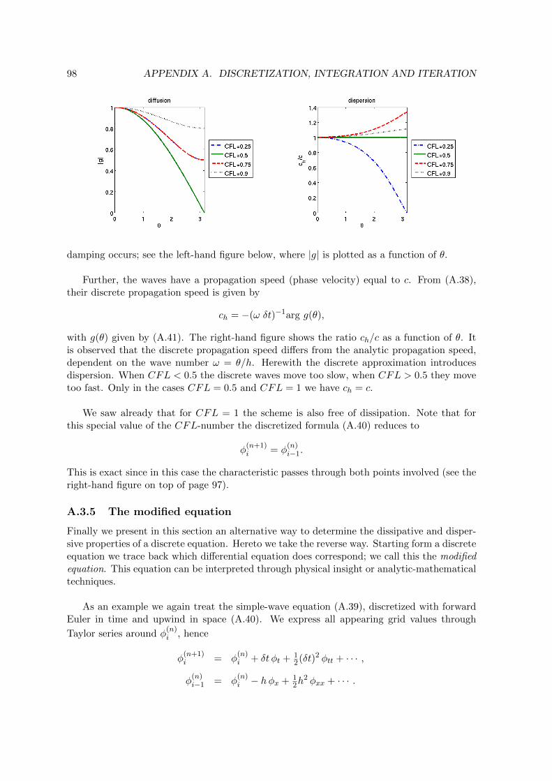
98 APPENDIX A. DISCRETIZATION, INTEGRATION AND ITERATION
damping occurs; see the left-hand figure below, where |g| is plotted as a function of θ.
Further, the waves have a propagation speed (phase velocity) equal to c. From (A.38),their discrete propagation speed is given by
ch = −(ω δt)−1arg g(θ),
with g(θ) given by (A.41). The right-hand figure shows the ratio ch/c as a function of θ. Itis observed that the discrete propagation speed differs from the analytic propagation speed,dependent on the wave number ω = θ/h. Herewith the discrete approximation introducesdispersion. When CFL < 0.5 the discrete waves move too slow, when CFL > 0.5 they movetoo fast. Only in the cases CFL = 0.5 and CFL = 1 we have ch = c.
We saw already that for CFL = 1 the scheme is also free of dissipation. Note that forthis special value of the CFL-number the discretized formula (A.40) reduces to
φ(n+1)i = φ
(n)i−1.
This is exact since in this case the characteristic passes through both points involved (see theright-hand figure on top of page 97).
A.3.5 The modified equation
Finally we present in this section an alternative way to determine the dissipative and disper-sive properties of a discrete equation. Hereto we take the reverse way. Starting form a discreteequation we trace back which differential equation does correspond; we call this the modifiedequation. This equation can be interpreted through physical insight or analytic-mathematicaltechniques.
As an example we again treat the simple-wave equation (A.39), discretized with forwardEuler in time and upwind in space (A.40). We express all appearing grid values through
Taylor series around φ(n)i , hence
φ(n+1)i = φ
(n)i + δt φt + 1
2(δt)2 φtt + · · · ,
φ(n)i−1 = φ
(n)i − hφx + 1
2h2 φxx + · · · .

A.4. REFERENCES 99
Substitution in (A.40) yields
φt + c φx = 12(c h φxx − δt φtt) + · · · . (A.42)
All time derivatives are transformed into spatial derivatives by using the differential equation(A.39), such as in
φtt = (φt)t = (−cφx)t = −c(φt)x = −c(−cφx)x = c2φxx.
Now (A.42) transforms to the modified equation
φt + c φx = 12c (1− CFL)hφxx + · · · . (A.43)
The right-hand side contains the difference with the equation that we wanted to solve. Werecognize a diffusive term. From PDE theory it is known that this equation is stable/unstablefor positive/negative diffusion, which (for c > 0) physically suggests the stability requirement0 ≤ 1− CFL. And this is indeed the correct numerical criterion.
A.4 References
E.F.F. Botta and A.E.P. Veldman (1982) On local relaxation methods and their application toconvection-diffusion equations. J. Comput. Phys. 48, 127–149.
A. Harten, J.M. Hyman and P.D. Lax (1976) On finite difference approximations and entropy con-ditions for shocks. Comm. Pure Appl. Math. 29, 297–322.
C. Hirsch (1990) Numerical Computation of Internal and External Flows, Volumes 1 and 2. JohnWiley.
R.A. Horn and C.R. Johnson (1991) Topics in Matrix Analysis. Cambridge University Press.
A.S. Householder (1964) The Theory of Matrices in Numerical Analysis. Blaisdell Publishing Com-pany (reprinted in 2006, Dover).
J.D. Lambert (1973) Computational Methods in Ordinary Differential Equations. John Wiley.
R.D. Richtmyer and K.W. Morton (1967) Difference Methods for Initial Value Problems. John Wiley.
A.E.P. Veldman (1996) Partiele Differentiaalvergelijkingen. Lecture notes (in Dutch), University ofGroningen.
E.L. Wachspress (1966) Iterative Solution of Elliptic Systems. Prentice Hall.
D.M. Young (1971) Iterative Solution of Large Linear Systems. Academic Press.

100 APPENDIX A. DISCRETIZATION, INTEGRATION AND ITERATION

Appendix B
Computer exercises
During the course several computer exercises have to be made. These exercises are to besolved in ‘pairs’ of one or two students. A (short) written report of the findings has to behanded in the following week; discussion of the homework with other ‘pairs’ of CFD studentsis not allowed during that period.
All software required for the exercises is available by downloading the files from the Nestorpages for this course:
Computational Fluid Dynamics > Course Information
An alternative is to download them through
http://www.math.rug.nl/∼veldman/Colleges/CFD/CFD-Exercises.html
B.1 Exercise 1 – Artificial diffusion
Files and commands Required files: cfd 1.m, cfd upw.m, ns exact.m
The program is started in Matlab with the command cfd 1.
Description
Consider the inhomogeneous convection-diffusion equation
dφ
dx− kd2φ
dx2= S on 0 ≤ x ≤ 1, with φ(0) = 0, φ(1) = 1.
The right-hand side is given by
S(x) =
2− 5x , 0 ≤ x ≤ 0.4,
0 , 0.4 < x ≤ 1.
In this exercise an upwind discretization of the above equation is applied. The discretesolution for three values of the diffusion coefficient k is plotted in one picture. Also the exactsolution for one value of k can be included in this picture.
101
102 APPENDIX B. COMPUTER EXERCISES
Questions
1. Firstly, study the discrete solution for a grid with N = 20 grid points, at the followingvalues of k: k = 0.1, 0.01 and 0.001. These values correspond with mesh-Peclet numbersP = 0.5, 5 and 50, respectively. One would expect (or at least hope) that these solutionstend to the (analytical) solution for k = 0. Hence, compare the discrete solutions tothe exact solution at k = 0 (ignore the Matlab warnings concerning division by zero).What do you observe; is there any such relation?
2. Next, compare the same three discrete solutions at k = 0.1, 0.01 and 0.001 (again forN = 20) to the exact solution at k = 0.025. Now, there seems to be some relationbetween the upwind limit for k → 0 and the exact solution at k = 0.025. Explain thisrelation.
3. Finally, study once more the upwind solutions at k = 0.1, 0.01 and 0.001, but now on agrid with N = 40 grid points. Which exact solution, i.e. at which value of k, correspondswith the upwind limit for k → 0?
B.2 Exercise 2 – Various discretization methods
Description
As in Exercise 1, we consider the inhomogeneous convection-diffusion equation
dφ
dx− kd2φ
dx2= S on 0 ≤ x ≤ 1, with φ(0) = 0, φ(1) = 1.
The right-hand side is given by
S(x) =
2− 5x , 0 ≤ x ≤ 0.4,
0 , 0.4 < x ≤ 1.
The Matlab file cfd 2 solves this equation with a number of finite-difference (-volume)methods. Several types of discretization are employed; the solutions obtained with thesediscretizations are shown in one combination figure – the exact solution is also indicated.Each figure shows eight smaller pictures, arranged as indicated below:
uniform grid upwind smart upwindlambda schemes B3 (λ = 1/2) QUICK (λ = 1/8) central (λ = 0)nonuniform grid upwind central A central B
Two types of grid are used: uniform grids and non-uniform (stretched) grids. Thestretched grid possesses N/2 equal grid cells between 0 and 1 − 5k, and N/2 equal gridcells between 1− 5k and 1.
The Matlab script also gives the eigenvalues of Method B; they are displayed in Matlab’smain window.

B.2. EXERCISE 2 – VARIOUS DISCRETIZATION METHODS 103
Required files
This exercise requires the files cfd 2.m, cfd upw.m, cfd lam.m, cfd cen.m, ns exact.m.
Questions to be solved on the computer
Compute the solutions for k = 0.05, k = 0.01 and k = 0.001 (i.e. P = 1, 5 and 50). Use agrid with N = 20 grid cells
1. Compare the upwind results with those of the ‘smart upwind’ method for the samevalues of k; give a personal opinion of the usefulness of the latter method in comparisonwith the ‘standard’ upwind.
2. Compare the results of the lambda-schemes (cf. Section 1.3.2) with those of the up-wind method; watch features like wiggle-dependency and artificial diffusion. Determineempirically for which value of k the QUICK method starts to wiggle, and explain this‘wiggle boundary’ theoretically (see Question 5 below).
3. Finally, consider the results on the stretched grid. Compare the upwind method andboth generalizations (A and B) of the central method (cf. Section 1.6). Describe thedifference between the discrete solutions; why has the upwind solution not improved?
4. On the stretched grid, determine empirically the value of k for which one of the eigen-values of the coefficient matrix of Method B crosses the imaginary axis. Furthermore,try to find a value of k for which the coefficient matrix is approximately singular. Watchhow the solution of Method B behaves at this singularity.
Questions to be solved by pencil-and-paper
5. Prove that λ ≥ max(12 −
kuh , 0) is a sufficient condition for the upwind-biased lambda
schemes from Eq. (1.15) on page 12 to be wiggle-free. In particular show that theQUICK method is wiggle-free for P ≤ 8/3. Hint: Try fundamental solutions of theform ri, and monitor the sign of r.
6. Discretize the convection-diffusion equation
dφ
dx− kd2φ
dx2= 0 on 0 ≤ x ≤ 1,
with Dirichlet boundary conditions
φ(0) = 0, φ(1) = 1.
Use a nonuniform grid with only one interior grid point at x = 1 − 2k; k remains anunspecified variable here. Use the discretization methods A and B. In both cases, A andB, solve the discrete system (which in fact is only one equation). Sketch both solutionsusing linear interpolation between the grid points. Compute the exact solution of theconvection-diffusion equation (at x = 1−2k) as well. Which discrete solution is better?

104 APPENDIX B. COMPUTER EXERCISES
B.3 Exercise 3 – The JOR and SOR method
Description
After discretization of a (system of) partial differential equation(s) one obtains a large systemof algebraic equations, Ax = b. Solving such a large system with a direct method is expensivewith respect to both memory and CPU time. Therefore, such systems are often solved withan iterative method.
As in Exercise 1 and 2, we consider the inhomogeneous convection-diffusion equation
dφ
dx− kd2φ
dx2= S on 0 ≤ x ≤ 1, with φ(0) = 0, φ(1) = 1.
The right-hand side is given by
S(x) =
2− 5x , 0 ≤ x ≤ 0.4,
0 , 0.4 < x ≤ 1.
The Matlab file cfd 3.m discretizes this equation with a number of finite-difference (-volume) methods, and solves the resulting linear systems iteratively.
Two types of grid are used: uniform grids and non-uniform (stretched) grids. Thestretched grid possesses N/2 equal grid cells between 0 and 1 − 5k, and N/2 equal gridcells between 1− 5k and 1. Several types of discretization are employed; on the uniform gridboth an upwind and a central discretization, and on the stretched grid an upwind, a centralA and a central B discretization are used.
The resulting linear systems are solved iteratively with the JOR and SOR methods. Asstopping criterion in these methods
‖ φn+1 − φn ‖∞≤ 10−5
is used, in which n is the counter of the iterative steps; the maximum norm of the differencebetween the solutions of two consecutive iteration steps must be sufficiently small.
Required files
This exercise requires the files cfd 3.m, plotev.m, plotsol.m, ns iterative.m, ns jor.m,
ns sor.m, ns exact.m.
Typing the command cfd 3 in Matlab starts a menu in which the choice of the grid,the discretization method, the iterative method and the value of the relaxation factor ωcan be given. Then, with the menu a program can be started which solves the convection-diffusion equation in the prescribed way. The results produced by the program consist of theeigenvalues of the Jacobi matrix, a plot of the iteration error (this error is written to thescreen as well), the total number of iterations and a plot showing the continuous solution, thediscrete solution computed with a direct solver and the discrete solution computed with theiterative method (provided the iterative method did converge).

B.3. EXERCISE 3 – THE JOR AND SOR METHOD 105
Questions to be solved on the computer
Compute the solution for k = 0.01. As a default, the program uses N = 10 grid cells.
1. Select the uniform grid; use first the upwind and then the central method. Determinenumerically whether the Jacobi method (i.e. the JOR method with ω = 1) convergesor not. Do the same for the Gauss-Seidel method (i.e. the SOR method with ω = 1).Put the results in the table below.
uniform Jacobi method Gauss-Seidel methodgrid convergent? # iterations convergent? # iterations
upwind
central
Use the eigenvalues of the Jacobi matrix, computed by cfd 3, to explain the results.When both methods converge, compare the convergence rate of the Jacobi and Gauss-Seidel method.
2. Select the uniform grid; use first the upwind and then the central method. Use various(suitably chosen) values of ω and determine numerically for each value of ω the numberof iterations needed by the JOR method. Determine in this way the optimal and max-imal relaxation factor, ωopt and ωmax, for the JOR method. Do the same for the SORmethod. Put the results in the table below.
uniform JOR method SOR methodgrid ωopt # it. ωmax # it. ωopt # it. ωmax # it.
upwind
central
Which systems are solved better by the JOR and SOR method, those resulting fromthe upwind discretization or those resulting from the central discretization?
3. Select the stretched grid; use first the upwind, then the central A and finally the centralB method. Determine numerically whether the Jacobi method (ω = 1) converges ornot. Do the same for the Gauss-Seidel method (ω = 1). Put the results in the tablebelow.
stretched Jacobi method Gauss-Seidel methodgrid convergent? # iterations convergent? # iterations
upwind
central A
central B

106 APPENDIX B. COMPUTER EXERCISES
Use the eigenvalues of the Jacobi matrix, computed by cfd 3, to explain the results.When both methods converge, compare the convergence rate of the Jacobi and Gauss-Seidel method.
4. Select the stretched grid: use first the upwind, then the central A and finally the centralB method. Use various (suitably chosen) values of ω and determine numerically for eachvalue of ω the number of iterations needed by the JOR method. Determine in this waythe optimal and maximal relaxation factor, ωopt and ωmax for the JOR method. Do thesame for the SOR method. Put the results in the table below.
stretched JOR method SOR methodgrid ωopt # it. ωmax # it. ωopt # it. ωmax # it.
upwind
central A
central B
In case of the central B discretization compare the discrete solution obtained with theJOR or SOR method with the discrete solution obtained with the exact solver. Dothe JOR and SOR method really converge? Use the eigenvalues of the Jacobi matrix,computed by cfd 3, to explain this result. Which systems are solved better by the JORand SOR method, those resulting from the upwind discretization, those resulting fromthe central A discretization or those resulting from the central B discretization?
Questions to be solved by pencil-and-paper
5. In Section A.3.1 for a central discretization on the uniform grid the Jacobi matrix andits eigenvalues are derived. The Jacobi matrix reads
diag[P
4+
1
2, 0,−P
4+
1
2],
(P is the mesh-Peclet number) and its eigenvalues µJ are given by
µJ =1
2
√4− P 2 cos(
iπ
N), i = 1, . . . , N − 1,
where N is the number of grid cells.Derive in a similar way for the upwind discretization on the uniform grid the eigenvaluesµJ of the Jacobi matrix. Show that these eigenvalues are real and between -1 and 1 forevery value of P .Hint: the eigenvalues of the tri-diagonal matrix diag(a, 0, c) are given by
µ = 2√ac cos(iπ/N), i = 1, . . . , N − 1.
6. For a central discretization on the uniform grid the eigenvalues of the Jacobi matrixare pure imaginary when P > 2. Let the largest pure imaginary eigenvalue be givenby µJ = iµI , with µI real. The optimal and maximal relaxation factor for the JORmethod are given by (cf. Section A.3.1)
ωJOR,opt =1
1 + µ2I
, ωJOR,max =2
1 + µ2I
.

B.4. EXERCISE 4 – TIME INTEGRATION 107
For an upwind discretization on the uniform grid the eigenvalues of the Jacobi matrixare real (see Question 5). Let the largest real eigenvalues be given by µJ = µR andµJ = −µR, with µR real. Derive, as a function of µR, the optimal and maximalrelaxation factor for the JOR method.Hint: the eigenvalues µJOR of the iteration matrix of the JOR method are related to
the eigenvalues µJ of the Jacobi matrix by µJOR = 1 + ω(µJ − 1), and the JORmethod converges when the eigenvalues µJOR lie within the unit circle.
Furthermore, for the SOR method give the optimal and maximal relaxation factor (as afunction of µI and µR respectively) when using the central and the upwind discretization.
7. Use Questions 5 and 6 (remember that k = 0.01 and N = 10) to determine for theJOR method the values of the optimal and maximal relaxation factor when solvingthe systems resulting from the discretization on the uniform grid with respectivelythe upwind and central method. Do the same for the SOR method. Compare thesetheoretical results with the numerical results from Question 2.
8. Consider the upwind discretization on the stretched grid. Use Question 6 (rememberthat k = 0.01 and N = 10) and the numerical values of the eigenvalues µJ of the Jacobimatrix, computed as a byproduct by cfd 3 in Question 4, to determine for the JORmethod the theoretical values of the optimal and maximal relaxation factor. Do thesame for the SOR method. Compare these theoretical results with the numerical resultsfor the upwind discretization on the stretched grid from Question 4.Why is it difficult to compute the theoretical optimal and maximal relaxation factorwhen solving the systems resulting from a discretization on the stretched grid with acentral A or central B method?
B.4 Exercise 4 – Time integration
Description
Consider the heat equation
∂T
∂t=∂2T
∂x2, 0 ≤ x ≤ 1, 0 ≤ t ≤ 4,
with boundary conditions
T (0, t) = 0 and∂T
∂x(1, t) = 0,
and initial conditionT (x, 0) = x.
This equation is solved with a finite-difference method on a grid with N grid points (N = 10or 20). The Neumann condition is discretized with a mirror point. The quantity T (1, t) ismonitored. As time-integration method the generalized Crank-Nicolson method is used. Thediscretized heat equation reads
Tn+1j − Tnj
δt= (1− ω)
Tnj+1 − 2Tnj + Tnj−1
h2+ ω
Tn+1j+1 − 2Tn+1
j + Tn+1j−1
h2.
The simulation program is available as Matlab file cfd 4.m.

108 APPENDIX B. COMPUTER EXERCISES
Required files
This exercise requires the file cfd 4.m.
Typing the command cfd 4 in Matlab asks for the input of the required parameters forthis exercise: N , ω (omega) and δt.
Questions to be solved on the computer
1) First consider the fully explicit method (ω = 0). Vary the number of grid points asN = 10 and N = 20. Solve the heat equation for various time steps, as indicated inthe table below. Monitor whether the time integration is stable. In Question 4 you areasked to explain the stability limit on the time step.
time step 0.001 0.00125 0.00126 0.0025 0.005 0.0051 0.01stable? stable? stable? stable? stable? stable? stable?
N=10
N=20
2) Next, use the Crank-Nicolson method (ω = 0.5) and the generalized Crank-Nicolsonmethod with ω = 0.6. Use N = 10. Set the time step δt at 0.05 and 0.5; see the tablebelow. For the larger time step the solution shows clear oscillations. Make a roughestimate for the damping factor (defined as the quotient of two successive amplitudes)of the oscillations.
time step δt = 0.05 δt = 0.5stable? stable? damping
ω = 0.5
ω = 0.6
3) Finally, again for N = 10, investigate the fully implicit method (ω = 1). Use the sametime steps as in Question 2. Observe whether or not the solution shows oscillations.
time step δt = 0.05 δt = 0.5stable? oscillations? stable? oscillations?
ω = 1.0
Questions to be solved by pencil-and-paper
4) First consider the fully explicit method (ω = 0). Carry out a Fourier analysis of thismethod. Determine the maximum allowable time step forN = 10 andN = 20. Comparethese stability limits with the empirical observations in Question 1.
5) Carry out a Fourier stability analysis of the generalized Crank-Nicolson method, anddetermine the amplification factor. Show that the generalized Crank-Nicolson methodis unconditionally stable for ω ≥ 0.5. Investigate how the amplification factor behaves

B.5. EXERCISE 5 – NAVIER–STOKES SOLVER 109
when δt → ∞. Now explain the oscillations visible in Question 2. How are theseoscillations influenced when ω is increased from 0.5 to 0.6? Give a possible explanationwhy the observed amplification factors in Question 2 are somewhat different from thetheoretical amplification factors computed in this Question.
6) Derive theoretically for which values of the Crank-Nicolson parameter ω the solution iswiggle-free. As a special case, explain why the fully implicit method (ω = 1) does notshow oscillations (see Question 3). Hint: Use the concept of a positive operator.
B.5 Exercise 5 – Navier–Stokes solver
General description
After semi-discretization with an explicit time-discretization method with two time levels, theNavier–Stokes equations can be written as
div un+1 = 0,
un+1 − un
δt+ grad pn+1 = Rn,
in which R = −(u.grad)u + ν div grad u consists of the convection and diffusion terms.Rewriting and combining these two equations gives
div grad pn+1 = div (un
δt+Rn), (1a)
un+1 = un + δt Rn − δt grad pn+1. (1b)
The fortran program cfd 5.f solves the Navier–Stokes equations.
Files and commands
This exercise requires the files cfd 5.f, cfd.in, liqdmenu.m, liqdplot.m, liqprint.m,
xplot.m.
The program cfd 5.f has to be compiled with the command gfortran -o cfd 5 -O
cfd 5.f (any other Fortran compiler, e.g. ifort, will also do). Then, the program can berun with the command ./cfd 5. This program needs the input file cfd.in, this file has to beadjusted to perform the different computations. The input file, with the parameter setting ofQuestion 0, is included at the end of this exercise. At the end of the input file an explanationof the different parameters is given.
The program writes output both to the screen and to files. The output to the screen firstgives the values of the parameters describing the problem, and then gives each (user specified)time interval the time, div u, the number of Poisson iterations and the horizontal velocitiesat three positions at the vertical center line of the domain (at the bottom, halfway, and at thetop). Furthermore, output is written to the files uvpf#.dat and config.dat. The outputfile config.dat contains a description of the grid. The output file uvpf#.dat contains thehorizontal and vertical velocity and pressure in each grid cell at a certain time. In the inputfile the user can specify whether the file uvpf#.dat is made each (user specified) time interval

110 APPENDIX B. COMPUTER EXERCISES
or only at the end of the computation.
The output files uvpf#.dat and config.dat are needed for the post-processing in Matlab.Typing the command liqdmenu in Matlab starts a menu with which the post-processing canbe controlled. With the upper part of the menu surface or contour plots of the (different)velocities, pressure, vorticity or streamfunction can be made and with the lower part of themenu a movie of these plots at consecutive time steps can be made. With the middle part ofthe menu plots of the (different) velocities or the pressure along horizontal or vertical sectionsof the domain can be made.
Part I: Treatment of div un
Description
The term div un = 0 in the semi-discretized Navier–Stokes equations can be treated in twoways. The first way is to maintain this term in the equations. In this case equations (1a) and(1b) have to be solved. However, when the Poisson equation is solved exactly, div un+1 = 0.Therefore, the second way is to substitute this in the right-hand side of equation (1a) in thenext time step (i.e. substitute div un = 0). In this case the following equations have to besolved
div grad pn+1 = div Rn, (2a)
un+1 = un + δt Rn − δt grad pn+1. (2b)
Consider the lid-driven cavity problem; the flow in a square cavity with constantly movinglid. This problem is a well known test case for numerical methods for solving the Navier–Stokes equations. The domain and boundary conditions of this problem are shown in thefigure below. We will solve the lid-driven cavity problem with ν = 0.01.
u = 1 v = 0
u = v = 0
u = v = 0 u = v = 0
0
1
1
Parameter setting in the input file
Since we solve the lid-driven cavity problem with ν = 0.01, set Nu=0.01 in the input file. Usea stretched grid with 16 cells in each direction, i.e. set iMaxUs=jMaxUs=18. Take smaller cellsat the boundaries of the cavity, set xpos=ypos=0.5 and stretching parameters cx=cy=-0.5.Discretize the convection terms with a central method, i.e. set Alpha=0.0.
Since the velocity at the top is prescribed, set top=8, Uin=1.0 and Vin=0.0 in the in-put file. Furthermore, since at the other boundaries we have no-slip conditions, set left=2,

B.5. EXERCISE 5 – NAVIER–STOKES SOLVER 111
right=2 and bottom=2.
Since the program was originally developed to compute non-stationary flows, it does notcontain a stopping criterion which checks whether a stationary solution is reached or not.Instead, the program stops when the simulation time is equal to a user prescribed time (TFin),take TFin=25. Set the time step at DelT=0.025 and the maximal allowed CFL number atCFLMax=0.5. The program automatically adjusts the time step such that the CFL number isbetween 0.4*CFLMax and CFLMax. In each time step the Poisson equation is solved withMILU. Use in the input file PrtDt=1 and uvp=0, i.e. every second output is written to thescreen and the velocity field is written to the file uvpf0001.dat at the end of the simulation.
Question 0: ‘exact’ solution
First the ‘exact’ solution is computed, i.e. the discrete steady solution on the given grid.Hereto set in the input file Divuv=1 (i.e. retain the term div un in the Poisson equation),StrtP=1 (i.e. use the previously found pressure as initial guess for the iterations in the newtime step) and ε = 10−3. Note that the solution has converged in time, and write the resultsat t = 25 in the table below. Note that this table directly matches the output of the program.
time div u # it. u bottom u mid u top
25
Questions without div un
First, substitute div un = 0 in the Poisson equation (i.e. set Divuv=0 in the input file).Hence, solve the Navier–Stokes equations in the form (2a) and (2b). In each of the followingquestions, put the output of the program at t = 20, 21, . . . , 25 in a table of the format givenbelow.
time div u # it. u bottom u mid u top
20
21
22
23
24
25
1) Use for the Poisson solver an accuracy ε = 10−1 and use as initial solution for thePoisson solver p = 0, i.e. start the Poisson solver from scratch.
a) Look what happens with the term div u in time. Furthermore, make a plot ofthe solution; e.g. use the post-processing menu in Matlab to view the flow, use theupper part of the menu to make a surface plot of the streamfunction. Also havea look at the absolute velocity (crange [0, 0.1]) and the vertical velocity. Repeatthe simulation with TFin=100. Does the velocity field converge?

112 APPENDIX B. COMPUTER EXERCISES
b) Now we will consider what happens with the divergence when δt → 0: will thisimprove the solution? Set (temporarily) DelT=0.0025 and CFLMax=0.05 in theinput file. Repeat the simulation (with TFin=25). Look what happens with theterm div u in time. Compare this with the behaviour of div u in Question 1a.Explain the results.
2) Use for the Poisson solver an accuracy ε = 10−3, and use as initial solution for thePoisson solver p = 0, i.e. start the Poisson solver from scratch. Look what happenswith the term div u in time. Furthermore, make various plots of the solution as in theprevious question. The solution has improved, but is it really accurate?
3) Use for the Poisson solver an accuracy ε = 10−3, and use as initial solution for thePoisson solver the solution from the previous time step. Look once more what happenswith the term div u in time. Are you satisfied now?
4) Use for the Poisson solver an accuracy ε = 10−1, and use as initial solution for thePoisson solver the solution from the previous time step. Once again, describe thebehaviour of div u in time.
Questions with div un
Next, retain the term div un in the Poisson equation (i.e. set Divuv=1 in the input file).Hence, solve the Navier–Stokes equations in the form (1a) and (1b).
5) Use for the Poisson solver an accuracy ε = 10−1 and use as initial solution for thePoisson solver p = 0, i.e. start the Poisson solver from scratch.
a) Look what happens with the term div u in time. How do you like the solution?
b) Now we will consider what happens with the divergence when we let δt → 0.Set (temporarily) DelT=0.0025 and CFLMax=0.05 in the input file. Repeat thesimulation. Look what happens with the term div u in time. Compare the resultswith those from Question 5a, and explain the differences.
6) Use for the Poisson solver an accuracy ε = 10−3, and use as initial solution for thePoisson solver p = 0, i.e. start the Poisson solver from scratch (set StrtP=0 in the inputfile). Look what happens with the term div u in time. Compare the results with thosefrom Question 5a, and explain the differences.
7) Use for the Poisson solver an accuracy ε = 10−3, and use as initial solution for thePoisson solver the solution from the previous time step (i.e. set StrtP=1 in the inputfile). Monitor div u in time, and make plots of the solution. Explain the results.
8) Use for the Poisson solver an accuracy ε = 10−1, and use as initial solution for thePoisson solver the solution from the previous time step. Monitor div u and plot thesolution. How do you like the results?
Summary We have seen that the various approaches give quite different results. In the lastquestion of this part you will have to decide which approaches give acceptable results.

B.5. EXERCISE 5 – NAVIER–STOKES SOLVER 113
9) In practical applications one is often satisfied when the final solution has an accuracyof two digits. Keeping this in mind, compare the results from the Questions 1 to 8 andgive your opinion about which approaches give acceptable results?
Part II: Influence of boundary conditions
Description
We will now consider the choice of boundary conditions at in- and outflow openings. Theinflow boundary usually does not lead to too many problems. However, the outflow boundaryis much more problematic. When at an outflow boundary the normal velocity is prescribedthen a boundary layer may be created.
Consider the flow in a channel of length 10 and height 1. At the left (inflow) boundarythe fluid flows into the channel with a horizontal velocity u = 1. At the upper and lowerboundary of the channel we impose no-slip conditions. The geometry and (part of) theboundary conditions are given in the figure below.
u = 1v = 0
u = v = 0
u = v = 0
→→→
We will use two types of boundary conditions at the right (outflow) boundary of thechannel. Firstly, we will prescribe a horizontal velocity u = 1 at the right (outflow) boundaryof the channel as well. Secondly, we will allow a free outflow, obtained by setting the pressureat 0, at the right (outflow) boundary. We will consider the influence of these boundaryconditions on the solution.
Parameter setting in the input file
Use a grid without stretching with 32 cells in x-direction and 17 cells in y-direction, i.e. useiMaxUs=34 and jMaxUs=19 and cx=cy=0.0 in the input file. Note that the length of thechannel is 10, i.e. Xmax=10. Discretize the convection terms with a central method, i.e. setAlpha=0.0.
At the left (inflow) boundary the velocity is prescribed, hence set left=8, Uin=1, andVin=0. Furthermore, at the upper and lower boundary no-slip conditions are imposed, i.e.set top=2 and bottom=2.
Maintain the term div un in the Poisson equation (i.e. solve the Navier–Stokes equationsin the form (1a) and (1b), set Divuv=1 in the input file). Solve the Poisson equation with anaccuracy ε = 10−4. The Poisson equation is solved with MILU. Use as initial solution for thePoisson solver the solution from the previous time step (i.e. set StrtP=1).
Simulate the flow in the channel for 15 seconds, that is set TFin=15 in the input file. Setthe time step at DelT=0.025 and the maximal allowed CFL number at CFLMax=0.1. Use in

114 APPENDIX B. COMPUTER EXERCISES
the input file PrtDt=1 and uvp=1, i.e. every second of the simulation output is written to thescreen and every second of the simulation the velocity field is written to a file uvpf#.dat (beaware: this takes a lot of memory).
In every question below, plot the flow at the first five seconds of the simulation andat the end of the simulation, i.e. at t = 1, 2, . . . , 5 and t = 15. Use the post-processingmenu in Matlab to plot the flow. Use the upper part of the menu to make a surface plotof the absolute velocity. Furthermore, use the middle part of the menu to make a plot ofthe horizontal velocity along the horizontal center line (i.e. j-plane=10). By using the ’hold’button in the menu the plots of the horizontal velocity along the horizontal center line att = 1, 2, . . . , 5 and t = 15 can be put in one figure. A boundary layer and irregularities of theflow can easily be seen in the second plot.
Questions with prescribed outflow
Firstly, prescribe a horizontal velocity at the right (outflow) boundary of the channel as well:u = 1 and v = 0 (i.e. set right=8 in the input file).
10) Simulate the flow for ν = 0.01. Make plots of the flow as described above. Describe andexplain the development in time of the horizontal velocity along the horizontal centerline.
11) Simulate the flow for ν = 0.005. Make plots of the flow as described above. Comparethe flow with the one computed in Question 10, and explain the differences.
12) Simulate the flow for ν = 0.001. Make plots of the flow as described above. Com-pare the flow with those computed in Question 10 and 11, and explain the differences.Furthermore, make a surface plot of the absolute velocity in which the vector plot isincluded (select in the menu ’arrows automatic’ instead of ’no velocity vectors’),and zoom first in on the x-interval [0,1] and then on the x-interval [9,10] (i.e. take’manual x-axis’ instead of ’automatic zoom’ and select the interval). Furthermore,make a plot of the horizontal velocity at the vertical section at the i-plane 32. Whathappens with the velocity at the upper and lower boundary?
Questions with free outflow
Secondly, allow at the right boundary of the channel a free outflow condition (i.e. set right=7in the input file).
13) Simulate the flow for ν = 0.01. Make plots of the flow as described above. Comparethe flow with the one computed in Question 10, and explain the differences. What isthe limit value of the horizontal velocity at the center line y = 0.5.When the flow is fully developed the (horizontal) velocity profile is a parabola. Computethis parabola theoretically. What is the theoretical value of the horizontal velocity of thefully developed flow at the center line y = 0.5. Compare this result with the numericalvalue. Also make a cross sectional plot of the horizontal velocity near the end of thechannel to check the parabolic profile.
14) Simulate the flow for ν = 0.005. Make plots of the flow as described above. Comparethe flow with those computed in Question 11 and 13, and explain the differences. What

B.5. EXERCISE 5 – NAVIER–STOKES SOLVER 115
is the limit value of the horizontal velocity at the center line y = 0.5. Compare thisnumerical value with the theoretical value computed in Question 13.
15) Simulate the flow for ν = 0.001. Make plots of the flow as described above. Comparethe flow with those computed in Question 12, 13 and 14 and explain the differences.What is the value of the horizontal velocity at the center line y = 0.5 at the end of thechannel. Explain why this numerical value of the horizontal velocity at the center liney = 0.5 differs from the theoretical value computed in Question 13. Also make a crosssectional plot of the horizontal velocity near the end of the channel to see the shape ofthe velocity profile: is it a parabola?
Repeat the simulation with a channel of respectively length 20 and length 50 (set firstXmax=20 and then Xmax=50), use TFin=50 in order to reach a steady-state solution; alsoincrease Imax (although it has little influence). Set uvp=0 in order to save memory. Makeonly at the end of the simulation (i.e. at t = 50) a plot of the horizontal velocity alongthe horizontal center line (i.e. j-plane=10). What is the limit value of the horizontalvelocity at the center line y = 0.5. Again make a cross sectional plot of the horizontalvelocity near the end of the channel to see the shape of the velocity profile: is it aparabola now? Find a physical explanation of the results.
Example input file
***** tank geometry *************************************************
Xmin Xmax Ymin Ymax
0.0 1.0 0.0 1.0
***** grid definition ***********************************************
iMaxUs jMaxUs cx cy xpos ypos
18 18 -0.5 -0.5 0.5 0.5
***** liquid properties *********************************************
Nu
0.01
***** boundary conditions and inflow characteristics ****************
left right top bottom UIn VIn
2 2 8 2 1.0 0.0
***** discretization ************************************************
Alpha Divuv
0.0 1
***** poisson iteration parameters **********************************
Epsi ItMax StrtP
1.0e-4 100 1
***** time step ****************************************************
TFin DelT CFLMax
25 0.025 0.5
***** print/plot control ********************************************

116 APPENDIX B. COMPUTER EXERCISES
PrtDt uvp
1.0 0
---------------------------------------------------------------------
***** E X P L A N A T I O N ************* E X P L A N A T I O N *****
---------------------------------------------------------------------
**TANK GEOMETRY**
Xmin, Xmax, Ymin, Ymax : position of boundaries of computational domain
**GRID DEFINITION**
iMaxUs (<=130), jMaxUs (<=130) : number of cells including mirror cells,
the number of ’real’ cells is iMaxUs-2, jMaxus-2
cx, cy : stretchparameters - 0=no stretch;
>0=smaller cells near position
indicated by xpos,ypos;
<0=smaller cells away from xpos,ypos
**LIQUID PROPERTIES**
Nu : kinematic viscosity
**BOUNDARY CONDITIONS AND INFLOW CHARACTERISTICS**
left,right,top,bottom : type of boundary condition
1=slip
2=no-slip
7=free outflow : as boundary condition the pressure
is set at 0
8=inflow : the velocities are prescribed
UIn,VIn : in case of inflow conditions, prescribed velocities
the sign of UIn/VIn corresponds to the x/y-direction (hence it
does not necessarily correspond to the inward pointing direction)
**DISCRETIZATION**
Alpha : upwind parameter, discretization of convection term
0 = central
1 = upwind
Divuv : treatment of divergence
0 = substitute div u^n=0 in Poisson equation
1 = maintain div u^n in Poisson equation
**POISSON ITERATION PARAMETERS**
Epsi : convergence criterion of Poisson solver
ItMax : maximal allowed number of iterations of Poisson solver
Strtp : initial field of Poisson solver
0 = zero field p=0
1 = solution from previous time step, p=poud;
**TIME STEP**
TFin : endtime of simulation
DelT : timestep (is adjusted during the simulation in order to
keep the CFL number smaller than CFLMax)
CFLMax : maximum allowed CFL number

B.5. EXERCISE 5 – NAVIER–STOKES SOLVER 117
** PRINT/PLOT CONTROL**
PrtDt : time between 2 small printouts (to the screen and a file)
uvp : velocity and pressure in Matlab format
0=only at end of computation (preferable)
1=at every small printout (takes a lot of memory)


