Department of Theoretical Geophysics & Mantle Dynamics University of Utrecht, The Netherlands Computational Geodynamics diffusion, advection and the FDM Cedric Thieulot [email protected]June 16, 2017
Transcript
Department of Theoretical Geophysics & Mantle DynamicsUniversity of Utrecht, The Netherlands
Computational Geodynamicsdiffusion, advection and the FDM
I many methods in geodynamics (FEM, FDM, FVM, Spectral, ...)I many languages (C, C++, fortran, python, matlab, ...)I research codes based on pre-existing librariesI writing one’s own code is fun but
I modularise & test for robustnessI strive for portabilityI commentI use structuresI optimiseI visualiseI benchmark
C. Thieulot | Introduction to FDM
3
IntroductionSources
I Becker and Kaushttps://earth.usc.edu/~becker/Geodynamics557.pdf
I Spiegelmanhttp://www.ldeo.columbia.edu/~mspieg/mmm/course.pdf
The content of this presentation is mostly based on Becker & Kaus.
The solution of PDEs by means of FD is based on approximatingderivatives of continuous functions, i.e. the actual partial differentialequation, by discretized versions of the derivatives based on discretepoints of the functions of interest.
C. Thieulot | Introduction to FDM
5
Finite Difference Method basicsFinite differences and Taylor series expansions
I Suppose we have a function f (x), which is continuous anddifferentiable over the range of interest.
I Let’s also assume we know the value f (x0) and all the derivativesat x = x0.
I The forward Taylor-series expansion for f (x0 + h), away from thepoint x0 by a small amount h gives
f (x0+h) = f (x0)+h∂f∂x
(x0)+h2
2!∂2f∂x2 (x0)+· · ·+
hn
n!∂nf∂xn (x0)+O(hn+1)
I We can express the first derivative of f by rearranging
∂f∂x
(x0) =f (x0 + h)− f (x0)
h− h
2!∂2f∂x2 (x0)− . . .
C. Thieulot | Introduction to FDM
6
Finite Difference Method basicsFinite differences and Taylor series expansions
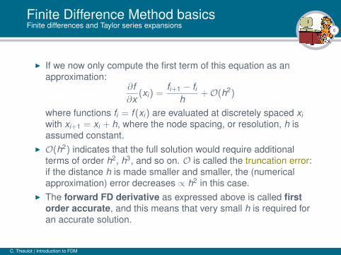
I If we now only compute the first term of this equation as anapproximation:
∂f∂x
(xi) =fi+1 − fi
h+O(h2)
where functions fi = f (xi) are evaluated at discretely spaced xiwith xi+1 = xi + h, where the node spacing, or resolution, h isassumed constant.
I O(h2) indicates that the full solution would require additionalterms of order h2, h3, and so on. O is called the truncation error:if the distance h is made smaller and smaller, the (numericalapproximation) error decreases ∝ h2 in this case.
I The forward FD derivative as expressed above is called firstorder accurate, and this means that very small h is required foran accurate solution.
C. Thieulot | Introduction to FDM
7
Finite Difference Method basicsFinite differences and Taylor series expansions
I We can also expand the Taylor series backward
f (x0 − h) = f (x0)− h∂f∂x
(x0) +h2
2!∂2f∂x2 (x0)− . . .
I The backward FD derivative then writes:
∂f∂x
(xi) =fi − fi−1
h+O(h2)
C. Thieulot | Introduction to FDM
8
Finite Difference Method basicsFinite differences and Taylor series expansions
Introducing the notations:
f ′ =∂f∂x
and f ′′ =∂2f∂x2
we can derive higher order derivatives:
f ′′i =f ′i+1 − f ′i
h=
fi+2−fi+1h − fi+1−fi
hh
=fi+2 − 2fi+1 + fi
h2 +O(h2)
which is the first order accurate, forward difference approximationfor second order derivatives around xi+1.
C. Thieulot | Introduction to FDM
9
Finite Difference Method basicsFinite differences and Taylor series expansions
I Alternatively, we can form the average of the first order accurateforward and backward schemes, and dividing by two.
I The result is the central difference approximation, secondorder accurate of the first derivative
f ′i =fi+1 − fi−1
2h+O(h3)
C. Thieulot | Introduction to FDM
10
Finite Difference Method basicsFinite differences and Taylor series expansions
I By adding the taylor expansions (with +h and −h) a secondorder accurate approximation of the second derivative isobtained
f ′′i =fi+1 − 2fi + fi−1
h2 +O(h3)
I Another way to arrive at the same expression:
f ′i+1/2 =fi+1 − fi
hf ′i−1/2 =
fi − fi−1
h
f ′′i =f ′i+1/2 − f ′i−1/2
h=
fi+1 − 2fi + fi−1
h2
C. Thieulot | Introduction to FDM
11
Finite Difference Method basicsDerivatives with variable coefficients
Note that derivatives with of the following form
∂
∂x
(k∂f∂x
)where k is a function of space, should be formed as follows
∂
∂x
(k∂f∂x
)∣∣∣∣i=
ki+1/2fi+1−fi
h − ki−1/2fi−fi−1
h
h+O(h3)
where ki±1/2 is evaluated between the points to maintain the secondorder accuracy.Note: If k has strong jumps from one grid point to another that are not aligned with the grid-nodes, most second-order methods will show
first order accuracy at best.
C. Thieulot | Introduction to FDM
12
Finite Difference Method basicsStencils
Stencils for the finite difference Laplacian operator, i.e., the geometricarrangement of points involved in calculating this discrete Laplacian.
C. Thieulot | Introduction to FDM
13
Solving the 1D heat equationExplicit approach
I Consider the one-dimensional, transient (i.e. time-dependent)heat conduction equation without heat generating sources
ρcp∂T∂t
=∂
∂x
(k∂T∂x
)where ρ is density, cp heat capacity, k thermal conductivity, Ttemperature, x distance, and t time.
I If the thermal conductivity, density and heat capacity areconstant over the model domain, the equation can be simplifiedto a diffusion equation:
∂T∂t
= κ∂2T∂x2
where κ = k/ρcp is the heat diffusivity.
C. Thieulot | Introduction to FDM
14
Solving the 1D heat equationExplicit approach
I The derivative of temperature w.r.t. time can be approximatedwith a forward finite difference approximation as
∂T∂t
=T n+1
i − T ni
tn+1 − tn =T n+1
i − T ni
δt
I n represents the temperature at the current time step whereasn + 1 represents the new (future) temperature. The subscript irefers to the location.
I Both n and i are integers; n varies from 1 to nstep (total numberof time steps) and i varies from 1 to nnx (total number of gridpoints in x-direction).
I The spatial derivative is replaced by a central FD approximation
∂2T∂x2 =
T ni+1 − 2T n
i + T ni−1
h2
C. Thieulot | Introduction to FDM
15
Solving the 1D heat equationExplicit approach
I We obtainT n+1
i − T ni
δt= κ
T ni+1 − 2T n
i + T ni−1
h2
and finally
T n+1i = T n
i + δt κT n
i+1 − 2T ni + T n
i−1
h2
I Because the temperature at the current time step n is known, wecan compute the new temperature without solving any additionalequations.
I Such a scheme is an explicit finite difference method and wasmade possible by the choice to evaluate the temporal derivativewith forward differences.
C. Thieulot | Introduction to FDM
16
Solving the 1D heat equationExplicit approach
I In order to solve this equation we need toI prescribe an initial temperature fieldI prescribe boundary conditions (T1 cannot be computed by means
of the above equation !)
I We know that this numerical scheme will converge to the exactsolution for small h and δt because it has been shown to beconsistent - that its discretization process can be reversed,through a Taylor series expansion, to recover the governingpartial differential equation - and because it is stable for certainvalues of h and δt : any spontaneous perturbations in the solution(such as round-off error) will either be bounded or will decay.
C. Thieulot | Introduction to FDM
17
Solving the 1D heat equationExplicit approach
I The main drawback of the explicit approach is that stablesolutions are obtained only when
0 <2κδth2 ≤ 1
or,
δt ≤ h2
2κI If this condition is not satisfied, the solution becomes unstable,
starts to wildly oscillate and ultimately ’blows up’.I The stability condition means that the maximum time step needs
to be smaller than the time it takes for an anomaly to diffuseacross the grid (nodal) spacing h.
I The explicit solution is an example of a conditionally stablemethod that only leads to well behaved solutions if a criterion likethe one above is satisfied.
C. Thieulot | Introduction to FDM
18
Solving the 1D heat equationImplicit approach
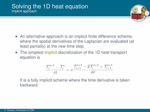
I An alternative approach is an implicit finite difference scheme,where the spatial derivatives of the Laplacian are evaluated (atleast partially) at the new time step.
I The simplest implicit discretization of the 1D heat transportequation is
T n+1i − T n
i
δt= κ
T n+1i+1 − 2T n+1
i + T n+1i−1
h2
It is a fully implicit scheme where the time derivative is takenbackward.
C. Thieulot | Introduction to FDM
19
Solving the 1D heat equationExplicit vs implicit approach
I The previous equation can be rearranged as follows:
−sT n+1i+1 + (1 + 2s)T n+1
i − sT n+1i−1 = T n
i
I Note that in this case we no longer have an explicit relationshipfor T n+1
i−1 , T n+1i and T n+1
i+1 . Instead, we have to solve a linearsystem of equations, which is discussed further below.
→ board: matrix structure and b.c.
C. Thieulot | Introduction to FDM
21
Solving the 1D heat equationImplicit approach
I The main advantage of implicit methods is that there are norestrictions on the time step, the fully implicit scheme isunconditionally stable.
I This does not mean that it is accurate. Taking large time stepsmay result in an inaccurate solution for features with small spatialscales.
I For any application, it is therefore always a good idea to checkthe results by decreasing the time step until the solution does notchange anymore (this is called a convergence check), and toensure the method can deal with small and large scale featuresrobustly at the same time.
C. Thieulot | Introduction to FDM
22
Solving the 1D heat equationImplicit approach
I Looking at
−sT n+1i+1 + (1 + 2s)T n+1
i − sT n+1i−1 = T n
i
and dividing by −s and letting δt →∞, we obtain:
T n+1i+1 − 2T n+1
i + T n+1i−1 = 0
which is a central difference approximation of the steady statesolution
∂2T∂x2 = 0
I Therefore, the fully implicit scheme will always yield the rightequilibrium solution but may not capture small scale, transientfeatures.
C. Thieulot | Introduction to FDM
23
Solving the 1D heat equationImplicit approach
I It turns out that this fully implicit method is second order accuratein space but only first order accurate in time, i.e. the error goesas O(h3, δt2).
I It is possible to write down a scheme which is second orderaccurate both in time and in space (i.e. O(h3, δt3)), e.g. theCrank-Nicolson scheme which is unconditionally stable.
I The Crank-Nicolson method is the time analog of central spatialdifferences and is given by
T n+1i − T n
i
δt=κ
2
[T n
i+1 − 2T ni + T n
i−1
h2 +T n+1
i+1 − 2T n+1i + T n+1
i−1
h2
]
C. Thieulot | Introduction to FDM
24
Solving the 1D heat equationImplicit approach
Any partially implicit method is more tricky to compute as we need toinfer the future solution at time n + 1 by solution (inversion) of asystem of linear equations based on the known solution at time n.
Crank-Nicolson stencil
C. Thieulot | Introduction to FDM
25
Solving the 1D heat equationImplicit approach
The implicit approach yields a linear system of the form:
A · T = b
where
I A is a nnx*nnx matrix,I b is a known vector of size nnx (the ’right-hand side’, or rhs)I T the vector of unknowns.
C. Thieulot | Introduction to FDM
26
Solving a linear system of equationsDirect solvers
I A general strategy to solve A · x = b is then LU decomposition:
A = L · U
where L and U are lower and upper triangular matrices,respectively, which only have zeros in the other part of the matrix.
I The solution of A · x = b can then be obtained efficiently from
L · U · x = b
by solving y = L−1 · b and then x = U−1 · y because the inverseof L and U are computationally fast to obtain. ’LU’ is often howgeneral matrix inversion is implemented on a computer.
C. Thieulot | Introduction to FDM
27
Solving a linear system of equationsDirect solvers
I For most FE/FD problems, the A matrix will be sparse andbanded.
sparse matrix sparse banded matrix
C. Thieulot | Introduction to FDM
28
Solving a linear system of equationsDirect solvers
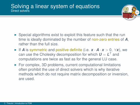
I Special algorithms exist to exploit this feature such that the runtime is ideally dominated by the number of non-zero entries of A,rather than the full size.
I If A is symmetric and positive definite (i.e. x · A · x > 0, ∀x), wecan use the Cholesky decomposition for which U = LT andcomputations are twice as fast as for the general LU case.
I For complex, 3D problems, current computational limitationsoften prohibit the use of direct solvers which is why iterativemethods which do not require matrix decomposition or inversion,are used.
C. Thieulot | Introduction to FDM
29
Solving a linear system of equationsDirect solvers
Solving a linear system of equationsIterative solvers
World of applied maths, computational science and linear algebra.
"The approximating operator that appears in stationary iterativemethods can also be incorporated in Krylov subspace methods suchas GMRES (alternatively, preconditioned Krylov methods can beconsidered as accelerations of stationary iterative methods), wherethey become transformations of the original operator to a presumablybetter conditioned one. The construction of preconditioners is a largeresearch area."https://en.wikipedia.org/wiki/Iterative_method
Solving a linear system of equationsIterative solvers - Jacobi method
I The simplest iterative solution of A · x = b is the Jacobi method.I If A is decomposed as A = L + D + U then an iterative solution
for x starting from an initial guess x0 can be obtained from
xk+1 = D−1 (b − (L + U) · xk)I A sufficient (but not necessary) condition for the method to
converge is that the matrix A is strictly or irreducibly diagonallydominant. Strict row diagonal dominance means that for eachrow, the absolute value of the diagonal term is greater than thesum of absolute values of other terms |aii | >
∑j 6=i |aij |
Note: this algorithm will fail if one or more diagonal terms of A is nul
C. Thieulot | Introduction to FDM
33
Solving a linear system of equationsIterative solvers - Gauss-Seidel method
I If A is decomposed as A = L + D + U then an iterative solutionfor x starting from an initial guess x0 can be obtained from
xk+1 = (L + D)−1 (b − U · xk)I The convergence properties of the Gauss–Seidel method are
dependent on the matrix A. Namely, the procedure is known toconverge if either:
I A is symmetric positive-definite, orI A is strictly or irreducibly diagonally dominant.
The Gauss–Seidel method sometimes converges even if theseconditions are not satisfied.
C. Thieulot | Introduction to FDM
34
Solving the 2D heat equationExplicit approach
I We now revisit the transient heat equation, this time withsources/sinks for 2D problems:
ρcp∂T∂t
=∂
∂x
(k∂T∂x
)+
∂
∂y
(k∂T∂y
)+ Q
where Q is the radiogenic heat production.I If the heat conductivity is constant, it writes:
∂T∂t
= κ
(∂2T∂x2 +
∂2T∂y2
)+
Qρcp
C. Thieulot | Introduction to FDM
35
Solving the 2D heat equationExplicit approach
C. Thieulot | Introduction to FDM
36
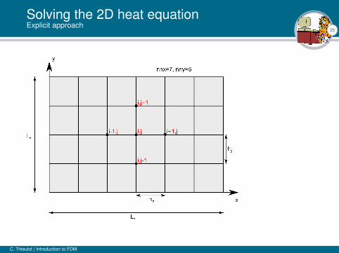
Solving the 2D heat equationExplicit approach
The simplest way to discretize the last equation on a domain, e.g. abox with width Lx and height Ly , is to employ an FTCS (forward time,centered space) explicit method like in 1D:
T n+1i,j − T n
i,j
δt= κ
(T ni−1,j − 2T n
i,j + T ni+1,j
h2x
+T n
i,j−1 − 2T ni,j + T n
i,j+1
h2y
)+
Qni,j
ρcp
We define sx and sy as follows:
sx =κδth2
xsy =
κδth2
y
so that
T n+1i,j = T n
i,j +sx(T ni−1,j−2T n
i,j +T ni+1,j)+sy (T n
i,j−1−2T ni,j +T n
i,j+1)+Qn
i,jδtρcp
C. Thieulot | Introduction to FDM
37
Solving the 2D heat equationExplicit approach
I The scheme is stable for
δt ≤min(h2
x ,h2y )
2κ
I Boundary conditions can be set the usual way. A constant(Dirichlet) temperature on the left-hand side of the domain (ati = 1), for example, is given by
Ti,j = Tleft ∀ j
C. Thieulot | Introduction to FDM
38
Solving the 2D heat equationImplicit approach
If we employ a fully implicit, unconditionally stable discretizationscheme as for the 1D exercise:
T n+1i,j − T n
i,j
δt= κ
(T n+1
i−1,j − 2T n+1i,j + T n+1
i+1,j
h2x
+T n+1
i,j−1 − 2T n+1i,j + T n+1
i,j+1
h2y
)+
Qni,j
ρcp
Rearranging terms with n + 1 on the left and terms with n on the righthand side gives
−sxT n+1i+1,j−sy T n+1
i,j+1+(1+2sx+2sy )T n+1i,j −sxT n+1
i−1,j−sy T n+1i,j−1 = T n
i,j+Qn
i,j
ρcp
which yields a linear system of equations written A · T = b where A isa (np × np) matrix.
C. Thieulot | Introduction to FDM
39
Solving the 2D heat equationExplicit approach
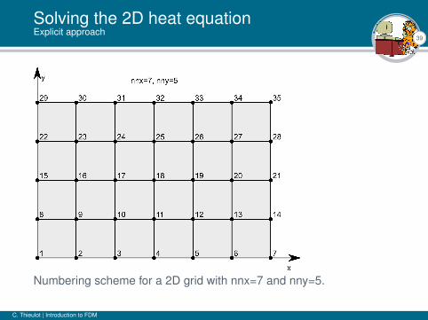
Numbering scheme for a 2D grid with nnx=7 and nny=5.
C. Thieulot | Introduction to FDM
40
Solving the 2D heat equationExplicit approach
Alternative numbering scheme for a 2D grid with nnx=7 and nny=5.
C. Thieulot | Introduction to FDM
41
Solving the 2D heat equationExplicit approach
Yet another alternative numbering scheme ...
C. Thieulot | Introduction to FDM
42
Solving the 2D heat equationExplicit approach
I In 2D we need a ’function’ which associates to every (i , j) aglobal index k .
I For the first grid: 1 ≤ i ≤ 7 , 1 ≤ j ≤ 5 so that 1 ≤ k ≤ 35
k = (j − 1) ∗ nnx + i
∂2T∂x2
∣∣∣∣i=3,j=4
=1h2
x(T2,4 − 2T3,4 + T4,4) =
1h2
x(T23 − 2T24 + T25)
Note that we now have five diagonals filled with non-zero entriesas opposed to three diagonals in the 1D case.
I More generally 1 ≤ i ≤ nnx , 1 ≤ j ≤ nny so that1 ≤ k ≤ np = nnx ∗ nny
C. Thieulot | Introduction to FDM
43
Other topics
I nonlinear coefficients, e.g. k = k(T )
I Neumann boundary conditions (heat flux as b.c.)I other stencilsI other schemes
C. Thieulot | Introduction to FDM
44
ExercisesEx.1
C. Thieulot | Introduction to FDM
45
ExercisesEx.1
Aim: building a 1D code which computes the temperature as afunction of time
I explicit vs explicitI timestep value ?I use the provided direct solver subroutineI build your own jacobi solver subroutineI try Crank-NicolsonI add a source term Q
C. Thieulot | Introduction to FDM
46
ExercisesEx.2
A simple (time-dependent) analytical solution for the temperatureequation exists for the case that the initial temperature distribution is
T (x , y , t = 0) = Tmax exp[−x2 + y2
σ2
]where Tmax is the maximum amplitude of the temperatureperturbation at (x , y) = (0,0) and σ its half-width. The solution is
T (x , y , t) =Tmax
1 + 4tκ/σ2 exp[− x2 + y2
σ2 + 4tκ
]Program the analytical solution and compare it with the explicit andfully implicit numerical solutions with the same initial conditions ateach time step. Comment on the accuracy of both methods fordifferent values of dt.
C. Thieulot | Introduction to FDM
47
The advection-diffusion equationPhilosophy
I So far, we mainly focused on the diffusion equation in anon-moving domain (relevant for the case of a dike intrusion orfor a lithosphere which remains undeformed).
I we now want to consider problems where material moves duringthe time period under consideration and takes temperatureanomalies with it (e.g. a plume rising through a convectingmantle).
I If the numerical grid remains fixed in the background, the hottemperatures should be moved to different grid points at eachtime step.
C. Thieulot | Introduction to FDM
48
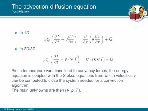
The advection-diffusion equationFormulation
I in 1D
ρcp
(∂T∂t
+ u∂T∂x
)=
∂
∂x
(k∂T∂x
)+ Q
I in 2D/3D
ρcp
(∂T∂t
+ v ·∇T)
= ∇ · (k∇T ) + Q
Since temperature variations lead to buoyancy forces, the energyequation is coupled with the Stokes equations from which velocities vcan be computed to close the system needed for a convectionalgorithm.The main unknowns are then (v ,p,T ).
C. Thieulot | Introduction to FDM
48
The advection-diffusion equationFormulation
I in 1D
ρcp
(∂T∂t
+ u∂T∂x
)=
∂
∂x
(k∂T∂x
)+ Q
I in 2D/3D
ρcp
(∂T∂t
+ v ·∇T)
= ∇ · (k∇T ) + Q
Since temperature variations lead to buoyancy forces, the energyequation is coupled with the Stokes equations from which velocities vcan be computed to close the system needed for a convectionalgorithm.
The main unknowns are then (v ,p,T ).
C. Thieulot | Introduction to FDM
48
The advection-diffusion equationFormulation
I in 1D
ρcp
(∂T∂t
+ u∂T∂x
)=
∂
∂x
(k∂T∂x
)+ Q
I in 2D/3D
ρcp
(∂T∂t
+ v ·∇T)
= ∇ · (k∇T ) + Q
Since temperature variations lead to buoyancy forces, the energyequation is coupled with the Stokes equations from which velocities vcan be computed to close the system needed for a convectionalgorithm.The main unknowns are then (v ,p,T ).
C. Thieulot | Introduction to FDM
49
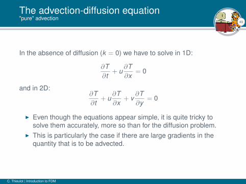
The advection-diffusion equation"pure" advection
In the absence of diffusion (k = 0) we have to solve in 1D:
∂T∂t
+ u∂T∂x
= 0
and in 2D:∂T∂t
+ u∂T∂x
+ v∂T∂y
= 0
I Even though the equations appear simple, it is quite tricky tosolve them accurately, more so than for the diffusion problem.
I This is particularly the case if there are large gradients in thequantity that is to be advected.
C. Thieulot | Introduction to FDM
50
The advection-diffusion equation"pure" advection
I If not done carefully, one can easily end up with strong numericalartifacts such as wiggles (oscillatory artifacts) and numericaldiffusion (artificial smoothing of the solution).
Thieulot, pepi 188, 2011.
C. Thieulot | Introduction to FDM
51
The advection-diffusion equation"pure" advection
I central difference scheme in space, and go forward in time(FTCS scheme):
T n+1i − T n
i
δt= −ui
T ni+1 − T n
i−1
2hx
where ui is the velocity at location i .
The FTCS method is unconditionally unstable !
i.e., it blows up for any δt .The instability is related to the fact that this scheme producesnegative diffusion, which is numerically unstable.
C. Thieulot | Introduction to FDM
51
The advection-diffusion equation"pure" advection
I central difference scheme in space, and go forward in time(FTCS scheme):
T n+1i − T n
i
δt= −ui
T ni+1 − T n
i−1
2hx
where ui is the velocity at location i .
The FTCS method is unconditionally unstable !i.e., it blows up for any δt .
The instability is related to the fact that this scheme producesnegative diffusion, which is numerically unstable.
C. Thieulot | Introduction to FDM
51
The advection-diffusion equation"pure" advection
I central difference scheme in space, and go forward in time(FTCS scheme):
T n+1i − T n
i
δt= −ui
T ni+1 − T n
i−1
2hx
where ui is the velocity at location i .
The FTCS method is unconditionally unstable !i.e., it blows up for any δt .The instability is related to the fact that this scheme producesnegative diffusion, which is numerically unstable.
C. Thieulot | Introduction to FDM
52
The advection-diffusion equation"pure" advection
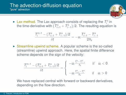
I Lax method. The Lax approach consists of replacing the T ni in
the time-derivative with (T ni+1 + T n
i−1)/2. The resulting equation is
T n+1i − (T n
i+1 + T ni−1)/2
δt= −ui
T ni+1 − T n
i−1
2hx
I Streamline upwind scheme. A popular scheme is the so-called(streamline) upwind approach. Here, the spatial finite differencescheme depends on the sign of the velocity:
T n+1i − (T n
i+1 + T ni−1)/2
δt=
−ui
T ni −T n
i−1hx
if ui < 0
−uiT n
i+1−T ni
hxif ui > 0
We have replaced central with forward or backward derivatives,depending on the flow direction.
C. Thieulot | Introduction to FDM
53
ExercisesEx.3
I Program the above FTCS methodI Change the sign of the velocity.I Change the time step and grid spacing and compute the
non-dimensional Courant number |u|δt/hx .I When do unstable results occur? Put differently, can you find a δ
small enough to avoid blow-up?I Program the Lax method by modifying the previous codeI Try different velocities and δt settings and compute the Courant
numberI Is the numerical scheme stable for all Courant numbers?I BONUS: Program the upwind scheme method. Is the numerical