Computational investigation of chain dynamics in ...digital.csic.es/bitstream/10261/137326/1/complex...

Computational investigationof chain dynamics in

architecturally complexpolymers

Petra Bacova

Thesis directors: Angel Jose Moreno Segurado and

Daniel Jon Read

PhD Thesis

Donostia-San Sebastian, July 2014

Acknowledgements

The Nobel physics prizewinner Leon Lederman said that ‘those whodo not stop asking silly questions become scientists’. Now, when I’mon my way to being a part of the scientific community, I would like toacknowledge all the people who helped me to find the answers for mynever ending questions.

First and foremost, I would like to express my deepest gratitude tomy supervisor Dr. Angel Moreno for patiently responding my commentsand doubts every day. Only thank to his immense support I was able toremove the obstacles that I encountered during my scientific adventure.I couldn’t have wished for a better supervisor. Angel, gracias por confiaren mı.

I also owe my deepest gratitude to my external supervisor Dr. DanielRead from the University of Leeds for his advices that have been es-sential during this work. Daniel, it was an honor for me to work withyou and learn from you during these four years.

I am indebted to my many of my colleagues from the Polymersand Soft Matter Group of the Materials Physic Center (CFM, CSIC-UPV/EHU), in particular to the head of the group, Prof. Juan Colmen-ero, for giving me the opportunity to be a part of this group. I would liketo thank to Federica, Zakaria and Marco for sharing with me not onlythe office but also useful ideas. Marco, grazie mille por ser mi familiade Leize Gorria. Leo, Guido, Gerardo, Fabienne, Eric y Pepe, graciaspor hacerme sonreır en los momentos cuando menos me apetecıa.

It was a great pleasure for me to be a part of the Marie Curie InitialTraining Network Dynacop. Many thanks to all students of Dynacopwho became my dearest friends and my unlimited source of motivation.My heartfelt appreciation goes to all professors and collaborative pro-fessors who achieved to provide us with necessary knowledge in veryshort time. I am very grateful to Prof. Peter Olmsted for his hospitalityduring my secondment. Thanks to Laurence, Stephen and Laurence’smum for making me feel at home during my stay in Leeds. I very much

ii

enjoyed working with Helen Lentzakis, Prof. Dimitris Vlassopoulos andChinmay Das, their inspiring comments and discussions were an enor-mous help to me.

I have greatly benefited from my HPC-EUROPA 2 visit in Stuttgart.I would like to thank to Dr. Axel Arnold and Dr. Olaf Lenz from theInstitute for Computational Physics in the University of Stuttgart, aswell as Dr. Alexey Cheptsov from the HLRS hosting team for theirhospitality and help with running ESPResSo on the supercomputers.

I also would like to thank to Dr. Christos Tzoumanekas for the usefuldiscussions about the role of entanglements in the polymer melts.

This thesis would have not been possible without the financialsupport from projects FP7-PEOPLE-2007-1-1-ITN (DYNACOP, EU),MAT2012-31088 (Spain) and IT654-13 (GV, Spain). I would like to ac-knowledge the programs PRACE, HPC-Europa2 and ESMI (EU), andICTS (Spain) for generous allocation of CPU time at GENCI (France),HLRS and FZJ-JSC (Germany) and CESGA (Spain).

Jedno obrovske DAKUJEM aj mojim najblizsım, ktorı to so mnoutie styri roky vydrzali. Bez vas by to neslo.

Abstract

We investigate the chain dynamics in the polymer melts with com-plex architecture by means of molecular dynamics simulations. Ourstudy is focused on the following architecturally complex polymers:T- and Y-shaped asymmetric stars, symmetric stars, mixtures of T-shaped asymmetric stars and linear chains, H-polymers, combs andCayley trees. Dynamics in these architectures is strongly influencedby the presence of one or more branchpoints. The overall chain dy-namics in branched structures is slowed down comparing to the linearchain and the relaxation of these materials extend over several timedecades. Extensive molecular dynamics simulations allow us to studythe relaxation processes ocurring in the branched polymer melts at themolecular level. We pay particular attention to the role of the branch-point in the dynamics of these systems. Our simulations reveal detailsabout the branchpoint motion that can be further compared to thetheoretical hypotheses, experimental data and finally introduced in thepredictions of the viscoelastic properties of the industrially producedmaterials.

The time evolutions of the mean squared displacements of the par-ticular molecular segments confirm that the arm retraction is the mainrelaxation mechanism in symmetric systems, i.e. symmetric stars andCayley trees. In these systems the branchpoint remains localized dur-ing the whole simulation time. We study the role of constraint releaseon the branchpoint dynamics and compare the simulation results witha theoretical model. The fluctuations of the branchpoint at time scalessmaller than the Rouse time τR are affected by the early tube dilationprocess that leads to a weaker branchpoint localization than expected.After the incorporation of the early and late tube dilation processesquantified from the simulation data into the theoretical model, we wereable to fully describe the branchpoint dynamics at the times smallerthan τR.

After the relaxation of the short side arms in the asymmetric struc-

iv

tures the arms act as sources of friction and the whole molecule canbe described as an effective linear chain. We studied the diffusion ofthe branchpoint after the arm relaxation. The calculation of the diffu-sion constant involves the knowledge about the arm relaxation, dilutionof the tube and the friction related to the reptation of the molecule.We estimated these observables from the simulations and tested theo-retical hypotheses used for the prediction of the branchpoint diffusivebehaviour in experimental studies of branched polymer melts.

We perform a detailed analysis of the branchpoint trajectories andpresent a robust method for finding regions of strong localization. Wecharacterize the time and length scales for the branchpoint motionbetween traps of localization, and discuss the consequences for the in-terpretation of the long-time branchpoint motion dynamics proposedby hierarchical tube models.

Contents

1 Introduction 1

1.1 Non-entangled vs. entanged polymers . . . . . . . . . . 11.2 Linear vs. architecturally complex polymers . . . . . . 61.3 Objectives and outline . . . . . . . . . . . . . . . . . . 9

2 Simulation method 13

2.1 Model and simulation details . . . . . . . . . . . . . . . 142.2 Systems and their preparation . . . . . . . . . . . . . . 19

3 Dynamics of symmetric systems 25

3.1 Relaxation mechanisms observed in MD simulations . . 253.2 Theoretical model . . . . . . . . . . . . . . . . . . . . . 30

3.2.1 Rouse dynamics . . . . . . . . . . . . . . . . . . 313.2.2 Entangled dynamics . . . . . . . . . . . . . . . 32

3.3 Quantitative evaluation of molecular dynamics data . . 363.3.1 Simulations with fixed chain ends . . . . . . . . 363.3.2 Simulations with free chain ends . . . . . . . . . 41

4 Dynamics of asymmetric systems 51

4.1 Diffusion of the branchpoint: theoretical background . . 514.2 Analysis of the simulation data . . . . . . . . . . . . . 55

4.2.1 Branchpoint displacement . . . . . . . . . . . . 554.2.2 Relaxation times . . . . . . . . . . . . . . . . . 564.2.3 Tube diameter and tube survival probability . . 594.2.4 Branchpoint trajectories . . . . . . . . . . . . . 67

4.3 Calculation of the hopping parameter . . . . . . . . . . 69

5 Real-Space Analysis of Branchpoint Motion 75

5.1 Heterogeneous branchpoint dynamics . . . . . . . . . . 755.2 Density-based cluster approach . . . . . . . . . . . . . 775.3 Analysis of the time and length scales . . . . . . . . . . 80

vi Contents

5.4 Discussion . . . . . . . . . . . . . . . . . . . . . . . . . 88

6 Conclusions 93

7 Publications 95

1. Introduction

In the last century, polymer materials definitely became a part ofour everyday life. Materials as glass, wood and iron were massively re-placed by different types of polymers with similar physical properties asthe substituted materials. Polymers are huge macromolecules composedof many repeating units (monomeric units) and the properties of thepolymer material strongly depend on the number of these units (N) aswell as on their spatial configuration [1]. Therefore, the understandingof the relation between the polymer structure and the material proper-ties is essential for the industrial processing and the design of the newpolymer products. The rheological behaviour of the melted polymershas been studied experimentally [2, 3, 4] and few theoretical modelswere developed to describe the dynamics of these systems [5, 6, 7, 8].To test the theoretical predictions, monodisperse model polymers withwell-defined architecture are needed. The progress in a controlled poly-mer synthesis [9, 10, 11] and in the simulation techniques [12, 13, 14]led to the improved description of the viscoelastic properties of thepolymer melts in recent years.

1.1 Non-entangled vs. entanged polymers

Let us consider a linear polymer melt. In a melt, segments of thesame and/or neighbouring chains are highly overlapped. Because ofthe covalent bonds between the monomeric units, chains can not passthrough each other and with the increasing chain length, polymers gettangled up. The topological constrains created in the system are calledentanglements and it is generally believed, that they are responsiblefor the exceptional viscoelastic properties of the entangled polymermelts [15]. The rheological properties of the non-entangled polymersdiffer significantly in comparison to the polymers chains in the entan-gled regime [16]. The melt viscosity η shows a general scaling behaviourwith respect to the molecular weight M of linear polymers of different

2 Chapter 1. Introduction

chemical composition [17]:

η ∼M1 M < Mc

η ∼M3.4 M > Mc.

The molecular weight Mc indicating the transition between the non-entangled and entangled regime is specific for each material and it islinked to the so-called entangled molecular weight Me:

Mc∼= 2Me.

This relation was held to be valid for a wide range of chemistries, untilit was showed recently, that the ratio of Mc and Me depends on thepacking length [18].

10-5 10-3 10-1 101 10310-3

10-1

101

103

105

PS642 PS732 PS742 PI254k PS652

G(t)

(Pa)

t (s)

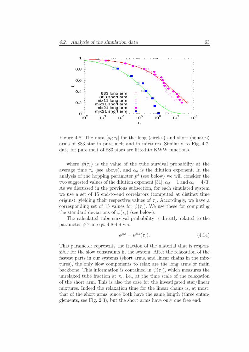
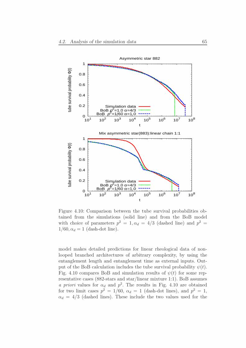
Figure 1.1: Experimental stress relaxation modulus G(t) as a functionof time for polystyrene (PS) and polyisoprene (PI) combs [19]. Thearrows indicate the arm relaxation times (for more details see [19]).

Viscosity is related to the stress relaxation modulus G(t) throughthe expression η =

∫∞0G(t)dt. The stress relaxation modulus contains

more information than the viscosity itself, it is a spectrum of the re-laxation processes occurring in the material [20]. It can be obtainedfrom the linear rheology measurements that record the response of thematerial to a step strain. While the relaxation of the non-entangledpolymers is fast and the terminal relaxation is detected at short timescales (high frequencies), a plateau appears before the final decay in

1.1. Non-entangled vs. entanged polymers 3

the relaxation spectrum of the long entangled chains [17] (Fig. 1.1). A(non-relaxing) plateau can be also observed in the polymer rubbers,where the chains ends are permanently cross-linked and the diffusionat the long time is disabled [17]. This fact confirms the importance ofthe entanglement constrains in the entangled polymer melts. However,the exact definition of the entanglements is unclear and the dynamicscoupled with their creation and/or removal has been widely discussedin the polymer community for decades [21, 22, 23].

Rouse model for non-entangled chains

The dynamics of non-entangled polymer chains can be described by

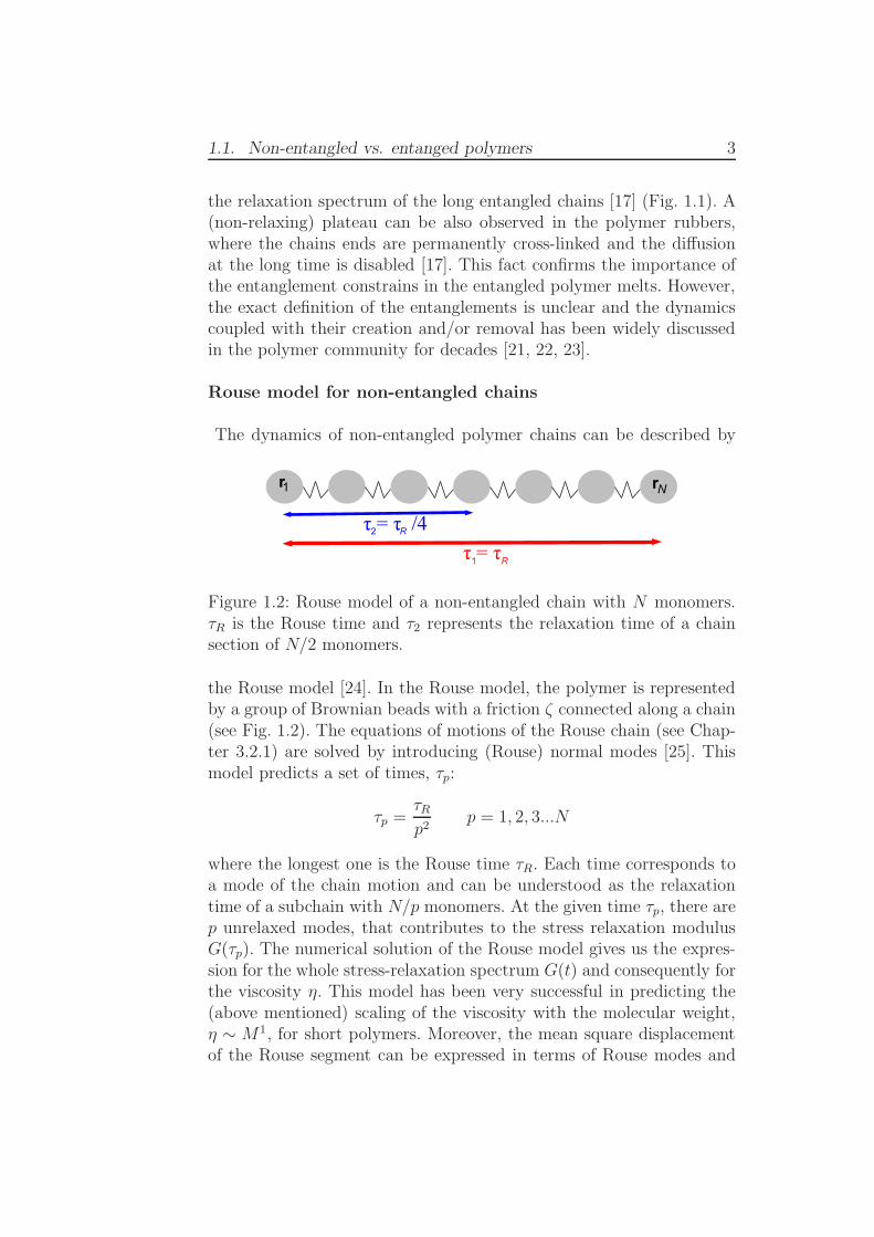
Figure 1.2: Rouse model of a non-entangled chain with N monomers.τR is the Rouse time and τ2 represents the relaxation time of a chainsection of N/2 monomers.

the Rouse model [24]. In the Rouse model, the polymer is representedby a group of Brownian beads with a friction ζ connected along a chain(see Fig. 1.2). The equations of motions of the Rouse chain (see Chap-ter 3.2.1) are solved by introducing (Rouse) normal modes [25]. Thismodel predicts a set of times, τp:

τp =τRp2

p = 1, 2, 3...N

where the longest one is the Rouse time τR. Each time corresponds toa mode of the chain motion and can be understood as the relaxationtime of a subchain with N/p monomers. At the given time τp, there arep unrelaxed modes, that contributes to the stress relaxation modulusG(τp). The numerical solution of the Rouse model gives us the expres-sion for the whole stress-relaxation spectrum G(t) and consequently forthe viscosity η. This model has been very successful in predicting the(above mentioned) scaling of the viscosity with the molecular weight,η ∼ M1, for short polymers. Moreover, the mean square displacementof the Rouse segment can be expressed in terms of Rouse modes and


this procedure leads to the following scaling regimes at short and longtimes:

〈r2(t)〉 ≃

(12kBTb2/πζ)

1/2t1/2 τN ≤ t ≤ τR,

6Dgt τR ≤ t

where kB is the Boltzmann constant, T temperature, τN is the relax-ation time of the fastest mode, b is the segmental length and Dg is thediffusion constant of the center-of-mass of the chain.

Tube model for entangled chains

Modelling of the entangled polymer melts is very challenging, because

Figure 1.3: Tube model. Left: entangled long polymer chains. Middle:surrounding chains treated as fixed obstacles (black circles) and thechain (orange line) restricted in the tube. The chain motion is pro-jected onto the primitive path (red line). Right: snake-like motion ofthe primitive path. The relaxed part of the original tube is drawn withdashed line.

one faces the problem of chains interacting by many-body interactions.The tube model intends to reduce the many-body problem to the pic-ture of a single-chain in an effective field [25]. In this model, the topo-logical constraints experienced by the chain in the melt are treated asfixed obstacles (black dots in the middle of Fig. 1.3), that restrict thechain motion in the tube-like region. Chain itself is represented by aprimitive path of length L (red curve in Fig. 1.3). Primitive path is theshortest path that connects the two chains ends and preserves the chaintopology, i.e. the uncrossability condition. The motion of the chain isprojected onto this path and on the long length-scales the primitivepath behaves as a random walk. One of the basic parameters of themodel is the tube diameter a, that corresponds to the end-to-end dis-tance of a chain of molecular weight identical to the entanglement massMe. Recently, molecular dynamics simulations showed that this param-

1.1. Non-entangled vs. entanged polymers 5

eter of the tube model should be understood as the tube Kuhn steplength rather than a real distance perpendicular to the tube axis [26].

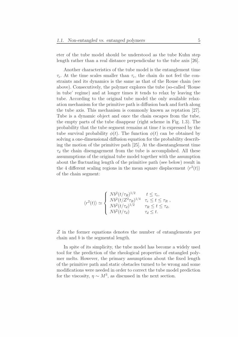
Another characteristics of the tube model is the entanglement timeτe. At the time scales smaller than τe, the chain do not feel the con-straints and its dynamics is the same as that of the Rouse chain (seeabove). Consecutively, the polymer explores the tube (so-called ‘Rousein tube’ regime) and at longer times it tends to relax by leaving thetube. According to the original tube model the only available relax-ation mechanism for the primitive path is diffusion back and forth alongthe tube axis. This mechanism is commonly known as reptation [27].Tube is a dynamic object and once the chain escapes from the tube,the empty parts of the tube disappear (right scheme in Fig. 1.3). Theprobability that the tube segment remains at time t is expressed by thetube survival probability φ(t). The function φ(t) can be obtained bysolving a one-dimensional diffusion equation for the probability describ-ing the motion of the primitive path [25]. At the disentanglement timeτd the chain disengagement from the tube is accomplished. All theseassummptions of the original tube model together with the assumptionabout the fluctuating length of the primitive path (see below) result inthe 4 different scaling regions in the mean square displacement 〈r2(t)〉of the chain segment:

〈r2(t)〉 ≃

Nb2(t/τR)1/2 t ≤ τe,

Nb2(t/Z2τR)1/4 τe ≤ t ≤ τR ,

Nb2(t/τd)1/2 τR ≤ t ≤ τd,

Nb2(t/τd) τd ≤ t.

Z in the former equations denotes the number of entanglements perchain and b is the segmental length.

In spite of its simplicity, the tube model has become a widely usedtool for the prediction of the rheological properties of entangled poly-mer melts. However, the primary assumptions about the fixed lengthof the primitive path and static obstacles turned to be wrong and somemodifications were needed in order to correct the tube model predictionfor the viscosity, η ∼M3, as discussed in the next section.


1.2 Linear vs. architecturally complex poly-

mers

The experimentally measured scaling of the viscosity with molecu-lar weight of the linear polymers, η ∼ M3.4, does not agree with thetheoretical prediction of the tube model, η ∼ M3. This discrepancyhas been explained by two additional relaxation mechanisms missingin the original tube model: constraint release (CR) and contour lengthfluctuations (CLF) of the primitive path [28, 29]. CLF correct the as-sumption about the fixed length of the primitive path and account forthe longitudinal fluctuations of the chain ends (see Fig. 1.4). It mustbe noted that these fluctuations do not include the center-of-mass (rep-tation) motion and affect the chain dynamics only at the time scalessmaller than τR. The CR mechanism describes the dynamic changes inthe entanglement network around a given chain that originate from themotion of the surrounding entangled chains. Each chain is not placed ina network of fixed obstacles, but the entanglements with neighbouringchains may appear and disappear. This leads to a reorganization of theoriginal tube, as it is illustrated in Fig. 1.4.

Most of the industrially produced polymer materials consist of poly-mers with branched or even hyperbranched architecture (e.g. LDPE). Inorder to describe the properties of these materials, the tube model hasbeen extended to model branched topologies like star polymers [30, 31],H-polymers [32, 33], pom-pom molecules [34], combs [35, 36, 37, 38, 2],Cayley trees [39, 40], DendriMacs [41] and topologies of industrial com-plexity [5, 42, 43]. These architecturally complex polymers contain oneor more branch points, that are responsible for their complex viscoelas-tic and dynamic properties as compared to linear chains [44]. Changingthe architecture from linear to branched has a huge effect on viscositythat increases exponentially with increasing number of entanglementsper arm, η ∼ exp(Ma/Me), with Ma the arm molecular weight and Me

the entanglement mass. Because of their complicated architecture, theG(t) spectrum of architecturally complex polymers is a combinationof many different relaxation mechanisms contributing to the overallrelaxation of the material.

Unlike in linear chains, reptation in branched systems remains in-active until the late stage of relaxation, or may be fully suppressed insymmetric architectures with a central branch point (e.g, Cayley trees).According to theory [15], relaxation before the onset of reptation occursvia arm retraction. The mechanism of arm retraction is analogous to

1.2. Linear vs. architecturally complex polymers 7

Figure 1.4: Schematic representation of the relaxation mechanisms inlinear and branched systems. Left: Constraint release (CR) and con-tour length fluctuations (CLF) in linear chains. Right: Dynamic tubedilution in stars. The original tubes are drawn with dashed lines, theconfiguration of the primitive path before the relaxation is illustratedby a red thick line. The obstacle shown with dashed grey line is re-moved and induces the reorganization of the tube indicated by greyarrow. The tube and primitive path configurations after relaxation aredepicted by cyan and blue lines respectively.

Figure 1.5: Schematic representation of the hierarchical relaxation inhyper-branched systems. Left: Unrelaxed molecule. Middle: Polymerafter the relaxation of the short outer segments. Relaxed side arms(highlighted with blue) act as friction beads (red circles). Right: Repta-tion of the effective linear chains with adjoint friction beads. The greyarrows indicate the retraction (left and middle) or reptation (right)mechanisms.

CLF in linear polymers, though involves deeper fluctuations and is ex-ponentially rare as relaxation approaches a branch point from the outer


segments. Topologies of industrial complexity which contain many lay-ers of branch points relax hierarchically [15, 5]. Hierarchical relaxationmeans that once free ends retract back to the outermost layer of branchpoints, these become mobile, activating deeper retractions towards thesecond layer, and so on. If the macromolecular architecture is asym-metric (e.g., T-shaped stars), the late relaxation occurs via reptationof an effective linear chain, in which all relaxed branches act as effectivefrictional beads (see Fig. 1.5). Regarding CR in branched polymers, theevidence for an extremely broad, exponential distribution of relaxationtimes gave rise to the tube dynamic dilution (DTD) hypothesis [15].In the DTD picture, at times longer than the relaxation time of outersegments, inner segments do not experience the entanglements with theouter ones, which have relaxed at much earlier time scales. This leads toa slow, progressive dilution of the effective entanglement network thatis modelled as a time-dependent widening (‘dilation’) of the tube (seeFig. 1.4). The dilated tube diameter at each time step is determinedby the respective fraction of relaxed material.

After incorporating the main features of the dynamics of the branchedpolymers into the tube model, the modified tube model is able to pre-dict qualitatively the rheological properties of these materials. Someproblems may arise while seeking for a quantitative agreement betweenthe theory and the experimental data. For example, due to the exponen-tial dependence of the relaxation time on the arm length, polydispersityof the material may change significantly the shape of the spectra [45].

Branchpoint dynamics

The missing piece of the puzzle in the theoretical predictions is the de-tailed description of the branchpoint motion. The direct experimentalaccess to the branchpoint motion is hard to be achieved, and reporteddata are still scarce [46]. In a pioneer work, Zhou and Larson [47] aimedto gain some information about the branchpoint dynamics by perform-ing molecular dynamics simulations of entangled star polymers. Visualinspection of the branchpoint trajectories revealed rather distinct fea-tures from inner segment motion in entangled linear chains. Whereasthe central part of the linear chain formed a diffuse trajectory along theconfined tube, the trajectories of the branchpoints in stars exhibited lo-calization regions. The branchpoint trajectories of the symmetric starswere mostly spherical, suggesting a strong localization of the branch-point in these systems. In case of the T-shaped asymmetric stars withslightly entangled short arm, the branchpoint trajectories were formed

1.3. Objectives and outline 9

by an alignment of various regions of localization. This feature wasrecognized as a signature of the hopping mechanism.

In the tube models hopping of the branchpoint is assumed to oc-cur after the relaxation of the side arms, when the branchpoint canprobe the space liberated by the removed constraints. The branchpoint,previosly localized, is then performing a random hop along the tube,whereas its diffusion is slowed down by the friction coming from therelaxed side arms. This fact is taken into account in the expression forthe branchpoint diffusion (eq. 4.1) through a dimensionless constantp2 called hopping parameter. It is assumed that the typical hoppingdistance is p times the tube diameter and that the value of p2 is of theorder of unity.

However, a series of investigations have suggested considerably smallervalues in the case of branched polymers with weakly or moderately en-tangled short arms [33, 48, 46]. Frischknecht et al. [49] found that,the drag caused by the relaxed short arms in asymmetric T-shapedstar polymers is much higher than the one predicted by the theory.In order to reproduce the experimental rheological data with hierar-chical tube-based models, the value of p2 needed to be adjusted de-pending on the length of the short arm. The values of the p2 obtainedfrom the comparison of the theory and rheological data varied in therange 1/4 ≤ p2 ≤ 1/60. In the experimental studies of H-polymers andcombs, the value of p2 was kept on fixed value 1/12 (firstly proposedin Ref [32]) and possible factors affecting the rheological spectra wereanalyzed [35, 36, 50, 51]. In addition, effects of architectural dispersityhave been recently considered and analyzed [52, 53, 54].

Instead of looking on the branchpoint friction, some studies usingslip-link simulations focused on the nature of the branchpoint motionitself. Shanbhag and Larson [55] suggested that the branchpoint dif-fusion is limited by the full removal of the entanglements around theshort arm. Masubuchi et al. [56] examined the relaxation mechanisms ofthe branchpoint and their contribution to the viscoelastic relaxation ofasymmetric stars. They observed that the more asymmetric the struc-ture is, the more relevant the contribution of branchpoint hopping be-comes for the overall relaxation of the star.

1.3 Objectives and outline

Though the tube model applied for the architecturally complexpolymers has gained general acceptance, the specific details of the pro-


posed mechanisms remain highly controversial. Verification of thesepostulated mechanisms is a frequently discussed topic in the polymercommunity [57, 58, 59, 60, 61]. While some of the hypotheses can betested by using experimental techniques and well-defined model poly-mers (e.g validity of the dynamic tube dilution theory [40, 62]), the pos-tulates related to the branchpoint motion remain unproven. Currentlyavailable experimental techniques are limitted to the short time scales(e.q. neutron spin echo [46]) and a direct observation of the branchpointdiffusion is not possible. Therefore, the branchpoint dynamics is one ofthe unresolved issues in the physics of entangled polymer melts. How-ever, due to the possibility of high paralelization in supercomputers,molecular dynamics simulations have become an extremely powerfultool for studying the behaviour of architecturally complex systems.

We performed extensive MD simulations on several branched ar-chitectures, including symmetric stars, asymmetric T-shaped and Y-shaped stars, combs, Cayley trees and mixtures of stars and linearchains. The simulations allow us to analyze directly the diffusive motionof the branchpoints without invoking specific assumptions for branch-point hopping. In this thesis work we aim to provide a detailed de-scription of the branchpoint dynamics that is essential for the full un-derstanding of the exceptional viscoelastic properties of the branchedpolymer materials. Moreover, we present an exensive study of the re-laxation processes occuring in these materials. We confront the resultsobtained from our simulations with the theoretical predictions and wego far beyond a simple testing of the tube-based theories.

1. We start with the symmetric structures, where the localization ofthe branchpoint is very strong and reptation of the molecule is not pos-sible. We focus on the dynamics of the branch point of the star polymerand of the central branch point of the Cayley tree, both in the presenceand absence of standard constraint release. The latter is achieved byperforming MD simulations with free and fixed chain ends, respectively.To provide a basic model with which to compare MD results, we havecollaborated with the group of Dr. Daniel Read (University of Leeds,United Kingdom), who derived analytical expressions describing localmotion of branched chains subject to entanglement constraints. Thetheoretical model consists in the unentangled case of the Rouse-likemodel adapted to star architectures. In the entangled case, the entan-glements are represented by localizing springs. We find that localiza-tion of the branch point in the simulations with fixed ends is weakercompared to the theoretical predictions, suggesting some relaxation ofthe entanglement constraints experienced by the branch point (e.g. an

1.3. Objectives and outline 11

early tube dilation process occurs). We quantify the standard CR bycomputing directly the tube survival probability from the MD. Finally,after the inclusion of CR events and early tube dilation in the theo-retical model, it provides an excellent description of the MSD of thebranch points within the simulation time window. This finding stronglysupports the physics underlying the ‘dynamic dilution’ hypothesis.

2. Then we continue with the analysis of asymmetric systems, wherethe relaxation of the side arms is followed by the branchpoint hoppingand the final relaxation is achieved by the backbone reptation with sidearms acting as effective friction beads. Obtaining the basic informationabout these relaxation mechanisms from the experiment is tricky, theprecise determination of the characteristic relaxation times can not beaccomplished without combining experiments and modeling. Therefore,there is a wide range of assumptions on branchpoint hopping introducedby hierarchical models that are used to interpret the rheological spectra.We use the results of the MD simulations on T-shaped and Y-shapedasymmetric stars, mixtures of asymmetric stars and linear chains, andcombs to shed light on the former picture of the relaxation in asym-metric systems. The direct observation of the branchpoint diffusion inthe simulations allows us to determine the friction of the branchpoints.We estimate the arm relaxation time, we observe the onset to the rep-tation regime in the branchpoint MSD and calculate the tube survivalprobability of all the systems. We pay particular attention to errors indetermining the different physical quantities measured by the simula-tions. We quantify the values of the hopping parameter p2 by using thetheoretical expressions proposed in hierarchical tube models, in par-ticular those developed by Daniel Read from the University of Leeds.By inserting the data from the simulation into these equations we testthe specific assumptions of the hierarchical models for branchpoint hop-ping. We rule out some commonly made assumptions that do not resultin broadly similar values of p2 across the different systems studied, i.e.they do not reflect the universal behaviour in architecturally complexsystems. We reach to an important conclusion, that the only consistentset of hopping parameters in the different architectures is achieved byincluding the contribution from the backbone friction, and consideringhopping in the dilated tube.

3. Finally, we return to the origin of all the theories about thebranchpoint hopping and we analyze the branchpoint trajectories ofall types of architecturally complex polymers. Without relying on thetube models, we perform a purely geometrical density-based clusteranalysis of the branchpoint trajectories and identify regions of strong


localization (‘traps’). We address the unresolved problem of the timeand length scales related to the hopping motion. The results revealthat there is actually no single hopping time (which definitely is notthe relaxation time of the side arm), but a wide distribution of timesdescribing the motion of the branchpoint within and between the traps.We estimate the typical (hopping) distance between the regions of lo-calization from the distribution of the distances between the traps.The analysis reveals some unexpected results, as the independence ofthe typical hopping distance on the strengh of tube dilution, and thepresence of strongly localized branchpoints at times much longer thanthe arm relaxation time, even in the case of very weakly entangled sidearms. We discuss the consequences of our analysis on the interpretationof the branchpoint diffusivity introduced by tube models.

The thesis memory is organized as follows. In the Chapter 2 wepresent the simulation model and discuss the simulation details. Wealso explain the equilibration method and the preparation of the sys-tems before the production run. In Chapter 3 we focus on the dynamicsof symmetric stars and Cayley trees. We describe the relaxation pro-cesses typical for these symmetric systems and analyze in detail thedynamics of the branchpoint at time scales smaller than τR. We con-firm the predictions based on the DTD picture. In Chapter 4 we turnour attention to asymmetric systems and the branchpoint diffusion atlong time scales. We present a critical analysis of the consistency of thedifferent model assumptions for branchpoint hopping. In Chapter 5 weintroduce a new geometrical method for the analysis of the branchpointtrajectories, and characterize the latter in terms of traps of localization.The thesis memory ends with the summary of the main conclusions.

2. Simulation method

On the long way to the full description of the viscoelastic proper-ties of the architecturally complex polymers, simulations act as a bridgebetween the experimentally measured properties and theoretical pre-dictions. Unlike the experiments, the simulation techniques are able toexplore the dynamic proceses at microscopic scales without the dificul-ties related to the synthesis of the model polymers [63]. In addition,we obtain from the simulations the information about the dynamicsof every part of the molecule, so the relaxation processes of particularpolymer segments can be analyzed separatelly, without any theoreticalmodel needed in the experimental techniques to interpret the complexrelaxation spectra.

Entangled polymer chains are huge macromolecules of the size ofhundreds of nanometers. A characterization of such immense objectsby fully atomistic simulations is very time consuming or even impossi-ble, because the data processed in the atomistic simulation include allchemical details. Fortunately, the information about the internal chem-ical structure is redundant in our study. We are interested in propertiesof polymer melts that are universal, independent of chemical details,but affected by some general polymer features (e.g. chain length, ar-chitecture). Therefore, we use a model that fits these requirements.The coarse-grained models as for example the bead-spring model rep-resent a very powerful tool, because they capture the general behaviourof entangled polymer materials observed in experiments by retainingthe common ingredients of these systems: monomer excluded volume,polymer-like architecture and chain uncrossability. During the coarse-graining procedure, some degrees of freedom are ignored and a polymerchain is represented as a simplified molecule [13, 64]. To be specific,in the bead-spring model the structure and dynamics at the lenghtscales smaller than 1 nanometer are omitted and the whole monomericunits are replaced by beads (see Section 2.1). This minimization of thenumber of coordinates leads to the significant reduction of the computa-

14 Chapter 2. Simulation method

tional time, thus simulations of these simplified models can be extendedalmost to the diffusive regime with the usage of current computationalresources.

There are two main classes of simulation techniques, Monte Carloand molecular dynamics simulations. In our study we combined bothof these two methods.

The polymer melts were prepared and equilibrated with the MonteCarlo procedure (see Section 2.2). The Monte Carlo algorithm is basedon random sampling, i.e. many random moves of the particles in thesample are performed in order to obtain an average value of the desiredobservable. The random moves are accepted and lead to the evolutionof the system when they meet a given criteria, usually set by a thermo-dynamics condition. In our case the given condition is related to thereduction of the local density fluctuations. Monte Carlo simulationsare especially useful for the polymer community in modelling of theproducts of polymer synthesis [65, 7] or in equilibrating large polymerstructures [66, 67, 68, 69, 70]. In Section 2.2 we present a Monte Carloprocedure called ‘prepacking’ that was recently developed for equili-bration of long entangled linear chains. We implemented this methodin the equilibration procedure of architecturally complex polymers.

After the equilibration, the molecular dynamics (MD) simulations(see section 2.1) were used to obtain detailed information about thedynamics of branched polymers in melt. Unlike the Monte Carlo simu-lations, the motion of particles in MD simulations is not random, butit is ruled throught equations of motion (eq. 2.4). The output of thesimulation is the time evolution of the particle positions. This informa-tion is further processed during the analysis of the polymer properties( Chapters 3 and 4).

2.1 Model and simulation details

Bead-spring model

The bead-spring model introduced by Kremer and Grest has becomea well-established model for the simulations of polymer melts [71]. Weused this coarse-grained model to simulate our architecturally com-plex polymers. In this model, the monomeric units along the chain arecoarse-grained into beads with a mass m0 and diameter σ, joined bysprings. The excluded volume interaction between the beads is pro-vided by a purely repulsive Lennard-Jones (LJ) potential, the so-called

2.1. Model and simulation details 15

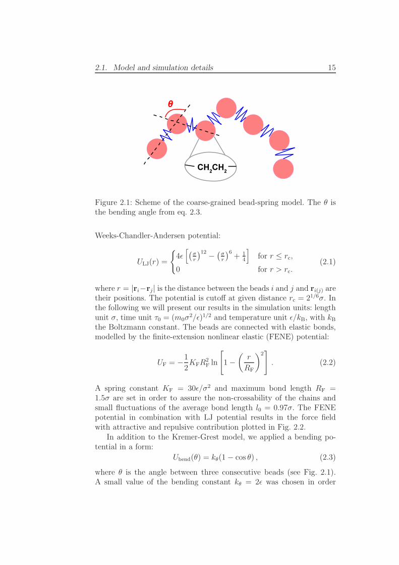
Figure 2.1: Scheme of the coarse-grained bead-spring model. The θ isthe bending angle from eq. 2.3.

Weeks-Chandler-Andersen potential:

ULJ(r) =

4ǫ

[(σr

)12 −(σr

)6+ 1

4

]for r ≤ rc,

0 for r > rc.(2.1)

where r = |ri−rj| is the distance between the beads i and j and ri(j) aretheir positions. The potential is cutoff at given distance rc = 21/6σ. Inthe following we will present our results in the simulation units: lengthunit σ, time unit τ0 = (m0σ

2/ǫ)1/2 and temperature unit ǫ/kB, with kBthe Boltzmann constant. The beads are connected with elastic bonds,modelled by the finite-extension nonlinear elastic (FENE) potential:

UF = −1

2KFR

2F ln

[1−

(r

RF

)2]. (2.2)

A spring constant KF = 30ǫ/σ2 and maximum bond length RF =1.5σ are set in order to assure the non-crossability of the chains andsmall fluctuations of the average bond length l0 = 0.97σ. The FENEpotential in combination with LJ potential results in the force fieldwith attractive and repulsive contribution plotted in Fig. 2.2.

In addition to the Kremer-Grest model, we applied a bending po-tential in a form:

Ubend(θ) = kθ(1− cos θ) , (2.3)

where θ is the angle between three consecutive beads (see Fig. 2.1).A small value of the bending constant kθ = 2ǫ was chosen in order


0

10

20

30

40

50

60

70

0 0.2 0.4 0.6 0.8 1 1.2 1.4 1.6

U(r)/

ε

r/ σ

LJ potentialFENE potential

FENE+LJ

Figure 2.2: FENE and LJ potentials as attractive and repulsive com-ponents of the effective force field between two mutually connectedmonomers (beads).

to increase slightly the chain stiffness. The characteristic ratio corre-sponding to this choice of the bending constant was obtained fromthe plot of the internal distances R(|n − m|) and was estimated asC∞ = 3.67±0.10 (see section 2.2). The semiflexible chains have a lowerentanglement length Ne then their flexible counterparts. It means thatthe chains with the particular length N create more entangled systemswhen their flexibility is moderated. This reduces computational costsince we can simulate well-entangled systems with a smaller number ofparticles than in the case of fully flexible polymers (kθ = 0). The entan-glement length estimated for the Kremer-Grest model with the givenbending potential (eq. 2.3) and kθ = 2 is Ne ≈ 25. This value is an aver-age of the entanglement lengths published in the literature obtained forthis model from two different methods. The first method includes theanalysis of the topological constraints in the system, so-called primitivepath analysis. This static approach gives NPP

e = 23 [72]. The secondmethod is based on the changes in dynamics of the middle monomerof linear chains. The entanglement length NMSD

e = 27 was estimatedfrom the monomer mean square displacement (MSD), specifically fromthe transition from MSD∝ t1/4 to MSD∝ t1/2 [47]. We must stress, thatthe introduction of the stiffness in our model does not play a role inthe further comparison with the theoretical models, that assume thechain Gaussianity. The chains are only slightly semiflexible and theircharacteristic ratio is even smaller than C∞ of typical industrial poly-

2.1. Model and simulation details 17

mers (C∞ = 5.20 for cis-polyisoprene [73]). The non-Gaussian effectsthat rise from the semiflexible character of the chains affect only thedynamics at the length scales smaller than the entanglement length.This can be checked from the plot of the internal distances R(|n−m|)(see Fig. 2.5). The plateau 〈R2(|n−m|)〉/|n−m|l20 ≈ C∞ expected forthe infinitely long Gaussian chain is already reached for the distances|n−m| ∼ Ne.

Simulation details

Our simulations are aimed to provide information about properties ofmacroscopic samples of polymer melts. However, the maximum num-ber of particles used in our simulation does not exceed 1.5 × 105 (seeFig. 2.3) and the current computational resources do not allow to sim-ulate significantly bigger systems. To avoid the finite size effects, theperiodic boundary conditions are activated in three directions in thesimulations. For more details see [74].

The choice of the size of the simulation cell was affected by two fac-tors. The length of the box has to be longer than the average maximal

distance between the ends of the molecule 〈R2e〉

1/2=

√ZNel20C∞, where

the number of entanglements in between the two ends Z is equal to 16for all the simulated systems (see Fig. 2.3). Moreover, we have to bearin mind that at least 100 molecules are needed to obtain good statis-tics in the analysis of the branchpoint dynamics. The total number ofbeads in a box, Nt, and its volume V were then adjusted according tothe relation for the typical number density of the melt in bead-springmodels ρn = Nt/V = 0.85σ−3.

All the simulations were performed at constant density, i.e. the boxvolume V and the total number of particles Nt in the box were constant.Moreover, a thermostat is introduced to maintain the average tempera-ture of the system at the desired value, in our case it is 〈T 〉 = ǫ/kB. Weused the Langevin thermostat with a friction constant Γ = 0.5m0/τ0,that has been proven to work well for polymer melts [71].

Equations of motion

In the molecular dynamics simulation the positions ri and momentapi = m0vi of the particles are propagated by the equations of motion.When the Langevin thermostat is implemented, the Newton’s equations


are replaced by the Langevin’s equations in this form:

dridt

=pi

m0,

dpi

dt= Fi − Γpi + Fr

i (t), (2.4)

Fi is the conservative force acting on a particle i, defined as the to-tal derivative of the potentials described by eqs. 2.1-2.3. Fr

i (t) is thestochastic force and the term Γpi represents the drag force. Thesetwo forces mimic the presence of a surrounding viscous medium inthe system, through the friction term (Γpi) and thermal kicks (Fr

i (t)).The variance of the random force Fr

i (t) is given by the fluctuation-dissipation theorem [25]:

⟨Fr

i (t) · Frj(t

′)⟩= 6kBTΓδijδ(t− t′), (2.5)

where δij is the Kronecker delta and δ(t− t′) the Dirac delta function.The equations of motion were integrated by the velocity-Verlet algo-

rithm [74]. This algorithm is implemented in ESPResSo in combinationwith the Langevin thermostat [75]. In every step of the integration, thealgorithm saves the information about the old positions and velocitiesat time t and updates the positions in the following manner [76]:

ri (t+∆t) = ri(t) + ∆tvi(t)

[1−∆t

Γ

2

]+

∆t2

2m0Gi(t), (2.6)

where Gi(t) is the total force Gi = Fi + Fri . Instead of the direct

calculation of vi (t+∆t), half step velocities are firstly introduced:

vi(t+1

2∆t) = vi(t)

[1−∆t

Γ

2

]+

∆t

2m0Gi(t). (2.7)

After this first stage of the integration, new forces at time (t + ∆t)are calculated. In this point one faces a technical problem, because thedrag force is velocity-dependent and thus the force calculation requiresthe velocity at time (t + ∆t), while we have only information abouthalf step velocities vi(t +

12∆t). However, if the dependence between

the forces and velocity is linear, one can assume that at time (t+∆t):

m0ai(t+∆t) = Gi(t+∆t)− Γvi(t+∆t)m0. (2.8)

The variable ai =dvi

dtin the former equation stands for the acceleration.

Moreover, the velocities can be updated by using the values of the halfstep velocities and the new accelerations:

vi(t+∆t) = vi(t +1

2∆t) +

∆t

2a(t+∆t). (2.9)

2.2. Systems and their preparation 19

By combining eq. 2.8 and eq. 2.9 we obtain the full set of expressionsneeded for the integration by the velocity-Verlet algorithm:

ai(t +∆t) =

Gi(t+∆t)m0

− Γvi(t+12∆t)

1 + Γ∆t2

(2.10)

vi(t+∆t) =

∆tGi(t+∆t)2m0

+ vi(t +12∆t)

1 + Γ∆t2

. (2.11)

The application of the Langevin thermostat has the advantage ofusing a relatively large time step, because the damping term stabilizesthe equations of motion. In the production run we used the step ∆t =0.01. On the other side, it must be noted that the stochastic termin the equations of motion leads to a drift of the simulation box intime, i.e., the momentum of the box is not zero. As a consequence,the displacements of the particles in time are biased. This fact has tobe taken into account during the calculation of the dynamic properties.Therefore in all our calculations the drift of the box was extracted fromthe particle positions.

2.2 Systems and their preparation

Simulated systems

In Fig. 2.3 the simulated architectures are schematically drawn. Wesimulated 3-arm symmetric and asymmetric stars, H-polymers, combs,Cayley trees and linear chains. The numbers labeling each part of themolecule in Fig. 2.3 represent the number of entanglements Z per eachbranch/backbone portion. The length of every part can be calculated asZNe, with Ne the number of monomers per entanglement segment. Themolecular span of all the systems is equal to 16 entanglements. The ar-chitectures of the simulated polymers were designed with the intentionto study the effect of topology on the dynamic properties of the mate-rials. In particular, the T-shaped 882 star and Y-shaped stars (Y2214and Y4212) differ in the possition of the short arm. The Cayley treehas a structure similar to the symmetric 888 star, the only differenceare the side arms placed in the middle of the long main arms. Similarly,the comb polymer is created by removing one of the three arms of theCayley tree. By comparing the dynamics of the Y-shaped asymmet-ric stars with the H-polymer and comb we can clarify the changes inthe viscoelastic properties of the materials with increasing number of


Figure 2.3: Scheme of the simulated systems: Ns represents the numberof branched polymers and Nc number of linear chains in the simulationbox. N is the number of beads per macromolecule. The red numbersplaced at each branch and backbone denote their lengths (Z) expressedin multiples of the entanglement length Ne = 25. Blue numbers expressthe composition of the mixtures, i.e. the ratio of the number of beadsbelonging to the asymmetric 883 stars to the total number of beads ofthe linear chains. In the text we refer to the particular system by itsbig black label.

branchpoints.

Equilibration

The first step of the molecular dynamics simulations is the prepara-tion of the system. This step is then followed by the equilibration andproduction run. The time required for the relaxation of entangled linearpolymer melts scales as N3.4 with the length N of the linear chain. Thusthe longer and more entangled are the simulated chains, the more diffi-cult is to prepare well-equilibrated systems. In the case of the branchedarchitectures the relaxation times are even longer (depending exponen-tially on the arm length, see Introduction). The equilibration of suchbig macromolecular systems as those shown in Fig. 2.3 with brute-force MD simulations is very far from being feasible with the currentcomputational capabilities. Therefore we followed recently developedequilibration methods, that combine Monte Carlo (MC) and MD sim-ulations.


Our equlibration procedure is based on the ideas introduced by Auhlet al. [66] for linear chains. First we prepared systems of small linearchains and 3-arm symmetric stars. The linear backbone and star armsare one entanglement length long. These unentangled polymer meltscan be easily equilibrated by brute force, i.e. we placed randomly themolecules in the box and run the molecular dynamics simulations tillthe static properties of the system fluctuated around a given averagevalue. Consequently, we used the equilibrated linear and star moleculesas building blocks to construct the systems presented in Fig. 2.3. Thebonds between building blocks were created as follows. The bendingangles at the junction points of different building blocks were chosenfrom the range (θmin; θmax). The maximum θmax of the chosen angle wasset to obey the equation 7 from [66] for the C∞ given for our model:

C∞ − 1

C∞ + 1= [cos(θmax/2)]

2. (2.12)

The lower limit was fixed as θmin = 0.75θmax. This constraint for thejunction angles guarantees the correct target function C([n − m|) =〈R2(|n − m|)〉/|n − m|l20 of the created architecture (see Ref. [66] fordetails).

Afterwards, the generated macromolecules were placed randomly inthe simulation box. Random orientation and position of the moleculesin the box can lead to overlaps of beads and regions with extremelyhigh density. This undesired effect can be eliminated by the prepackingprocedure [66]. The prepacking procedure consists of a Monte Carlosimulation in which the macromolecules are treated as rigid objectsperforming large-scale motions. These motions include rotations, trans-lations, reflections, inversions, and exchanges of two molecules pre-serving their center-of-mass positions. The Monte Carlo moves are ac-cepted only when they reduce the local density fluctuations [66]. Thereduction of the local density fluctuations is quantified by the variableE = 〈n2

b〉−〈nb〉2, related to the number of particles nb found in a sphereof radius d around every particle. During the prepacking procedure, thevalue of d is lowered from the initial value 4σ to the final value 2σ, asit was reported in [66]. The Monte Carlo simulation is stopped whenthe acceptance of the Monte Carlo moves is approaching zero, i.e. fur-ther moves do not lead to reduction of the local inhomogeneities. Thewhole procedure starting from the linking of the building blocks till theprepacking procedure is illustrated in Fig. 2.4.

Even if we eliminated the major part of overlapping beads duringthe prepacking procedure, a small amount of beads placed very close to


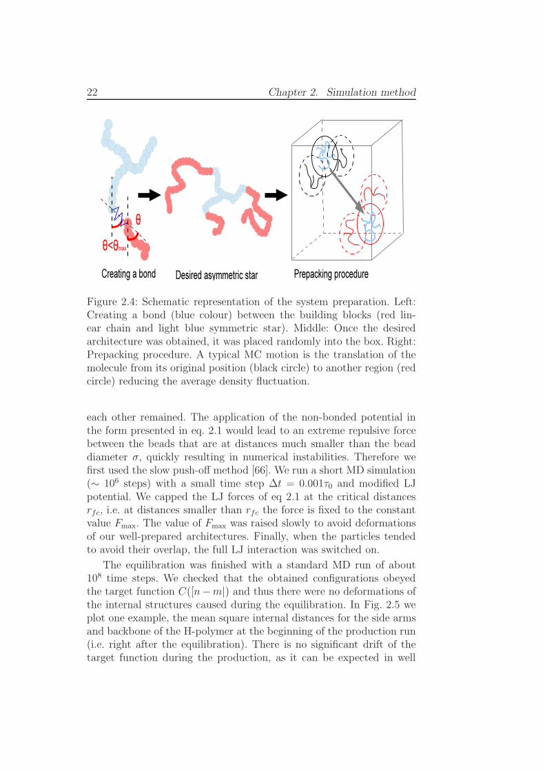
Figure 2.4: Schematic representation of the system preparation. Left:Creating a bond (blue colour) between the building blocks (red lin-ear chain and light blue symmetric star). Middle: Once the desiredarchitecture was obtained, it was placed randomly into the box. Right:Prepacking procedure. A typical MC motion is the translation of themolecule from its original position (black circle) to another region (redcircle) reducing the average density fluctuation.

each other remained. The application of the non-bonded potential inthe form presented in eq. 2.1 would lead to an extreme repulsive forcebetween the beads that are at distances much smaller than the beaddiameter σ, quickly resulting in numerical instabilities. Therefore wefirst used the slow push-off method [66]. We run a short MD simulation(∼ 106 steps) with a small time step ∆t = 0.001τ0 and modified LJpotential. We capped the LJ forces of eq 2.1 at the critical distancesrfc, i.e. at distances smaller than rfc the force is fixed to the constantvalue Fmax. The value of Fmax was raised slowly to avoid deformationsof our well-prepared architectures. Finally, when the particles tendedto avoid their overlap, the full LJ interaction was switched on.

The equilibration was finished with a standard MD run of about108 time steps. We checked that the obtained configurations obeyedthe target function C([n−m|) and thus there were no deformations ofthe internal structures caused during the equilibration. In Fig. 2.5 weplot one example, the mean square internal distances for the side armsand backbone of the H-polymer at the beginning of the production run(i.e. right after the equilibration). There is no significant drift of thetarget function during the production, as it can be expected in well


equilibrated systems.The 〈R2(|n−m|)〉/|n−m| function can be used for the estimation of

the chain stiffness. In particular, the average value of the characteristicratio can be extracted from the plateau of the average target function.For this purpose we chose the configurations of 888 symmetric stars,because in this case the statistics can be improved by averaging the tar-get functions over 3 equal star arms. We calculated the average targetfunction from 20 partial target functions collected at different times ofthe simulation run. This function together with the error bars is shownin Fig. 2.5 (red points). The average value of C∞ was then determinedfrom the long-distance plateau C∞l

20. In order to avoid possible sta-

tistical effects of the end fluctuations (the larger the distance betweenbeads |n − m|, the less pairs available in the average procedure), wedid not take into account the points of the average target function atthe distances bigger than 150. The estimated value of the characteristicratio was C∞ = 3.67 ± 0.10. The time step for this last equilibrationrun as well as for the production runs was ∆t = 0.01τ0.

0.5

1

1.5

2

2.5

3

3.5

4

1 10 100

<R2 (|n

-m|)>

/|n-m

|

|n-m|

target function, 888H-polymer, backbone

H-polymer, short arms

Figure 2.5: Mean square internal distances for the H-polymer at thebeginning of the production run (i.e. right after the equilibration). Thedata for the short arms were averaged over 4 equal side arms. Dashedlines set bounds to the mean value of characteristic ratio C∞ = 3.67±0.10 multiplied by the squared bond length l20. The mean value of C∞was estimated from the plateau C∞l

20 of the target function for the 888

star (red points) averaged over 20 partial target functions calculatedat different times of the simulation run.

Monte Carlo runs were performed serially (duration approximately


1 month), MD equilibration runs were performed only with low paralel-lization (up to 8 processors). All the simulation runs were performedby using the ESPResSo simulation package [75] and analyzed by ourhome-made codes. We use the ergodic hypothesis in the analysis andassumed that the average of a given variable over time and the averageover the statistical ensemble are the same [74]. Therefore, we performedaverage of observables over different time origins of the same run. Theergodic hypothesis is only valid in well-equilibrated systems (see abovefor more details about the proper equilibration). The production runswere performed by the use of supercomputer devices. High paralleliza-tion was needed to reach the long time regime (typically up to 4× 109

MD steps). The estimated total CPU time for the production runs wasof 3.5× 106 core-hours. Runs were performed at supercomputers Curie(PRACE program), CESGA, HLRS (HPC-Europa2 program) and JU-ROPA (ESMI program).

3. Dynamics of symmetric

systems

In this chapter we investigate the dynamics of polymers with lin-ear, symmetric star-like and Cayley tree-like topology. Cayley treesand 888 stars belong to symmetric systems, because the structure andlength of the three arms stemming from each central branch point arethe same (see Fig. 2.3). The linear chain can be treated as a 2-armstar with equally long arms. We analyze dynamic tube dilution byconfronting simulation results with a theoretical model developed byLaurence Hawke and Daniel Read (University of Leeds).

3.1 Relaxation mechanisms observed in MD

simulations

We start with the description of the relaxation mechanisms of thestudied systems obtained directly from the simulation data. The timeevolution of the monomer mean square displacement (MSD), 〈∆r2(t)〉,provides valuable information about the microscopic dynamics of thesystem. This quantity, which is often difficult to access in experiments,can be easily computed from the simulation data. Moreover, by com-puting the MSD of specific segments along the macromolecule, we mayshed light on the role of the macromolecular architecture on the inter-nal relaxation mechanisms. In our analysis of the simulation data, wehave divided the macromolecules into segments of length equal to oneentanglement (Ne = 25 monomers). The corresponding MSD of differ-ent segments in the three investigated systems are shown in Figs. 3.1and 3.2. We note that in Figs. 3.1 and 3.2 the time axis is expressedin simulation units τ0. The notations in the legends for the differentdata sets must be understood as follows. We treat the linear chain asa 2-arm star with the branch point in the center of the backbone, i.e.,

26 Chapter 3. Dynamics of symmetric systems

the arms have Z = 8 entanglement segments, as in the 3-arm stars. Welabel the entanglement segments in each arm of the linear chains andstars as e = 1, 2, ...8, by following the path from the branch point tothe outermost monomer in the same arm. Obviously, for each entangle-ment segment in a given arm there are, by symmetry, other equivalentsegments in the other arms and accordingly the corresponding MSDis averaged over them. In the case of the Cayley trees we do not in-clude in Fig. 3.2 the data for the short side branches (Z = 2), and theentanglement segments are labelled in the same way as in the linearchains and stars. Thus, we label the segments as e = 1, 2, ...8, by fol-lowing the path of length Z = 4 from the central branch point to oneof the three outer ones, and from there to the outermost monomer inthe same branch of Z = 4 (see Fig. 2.3). Again, the MSD is averagedover equivalent segments in the three long arms.

1

10

100

1000

10 100 1000 10000 100000 1e+06 1e+07

<∆r2 >

t

t0.6

linear e=1linear e=2linear e=3linear e=4linear e=5linear e=6linear e=7linear e=8

star e=1star e=2star e=3star e=4star e=5star e=6star e=7star e=8

Figure 3.1: MSD of the entanglement segments (see text) in the linearchains and symmetric stars.

In Fig. 3.1 we compare data of the linear chains and symmetricstars. In Fig. 3.2 the comparison is done for the linear chains and Cayleytrees. Up to the entanglement time τe ≈ 1800 (see Ref. [47]), the MSDof the different segments follow Rouse behaviour. The data are betterdescribed by an effective power-law 〈∆r2〉 ∼ t0.6 than by the strictlyRouse-like behaviour 〈∆r2〉 ∼ t1/2. This small difference may originatefrom non-Gaussian correlations (not included in the Rouse model) atN < Ne, which are related to the semiflexible character introduced bythe bending potential (eq. 2.3).

At the entanglement time τe ≈ 1800 the different segments start to

3.1. Relaxation mechanisms observed in MD simulations 27

1

10

100

1000

10 100 1000 10000 100000 1e+06 1e+07

<∆r2 >

t

t0.6


Cayley e=1Cayley e=2Cayley e=3Cayley e=4Cayley e=5Cayley e=6Cayley e=7Cayley e=8

Figure 3.2: MSD of the entanglement segments (see text) in the linearchains and Cayley trees.

probe the topological constraints, and the MSD progressively deviatesfrom the Rouse behaviour. In the usual picture for linear chains, the ini-tial fluctuations of the monomer along the primitive path are describedas Rouse dynamics of the curvilinear coordinate (‘Rouse in tube’ dy-namics) [77]. The consequence of this for the real-space monomer dy-namics is that the MSD scales as 〈∆r2(t)〉 ∼ t1/4. As aforementioned,the Rouse regime 〈∆r2(t)〉 ∼ tx in our system is characterized by anexponent x = 0.6 instead of the ideal value x = 1/2. Accordingly, wemay expect that the characteristic exponent for the ‘Rouse in tube’ dy-namics is x = 0.3 instead of the ideal value x = 1/4. Figs. 3.3 and 3.4show the ratio 〈∆r2(t)〉/t0.3. In this representation the ‘Rouse in tube’regime is recognized as a plateau for t > τe. Most of the segments inthe three investigated architectures exhibit this behaviour for at leasta portion of the time window τe < t < τR, where τR is the Rouse time,i.e., the time scale for the longest internal chain modes [25]. This canbe estimated as τR = τe(Na/Ne)

2 ≈ 105, with Na = 200 the number ofmonomers per long arm. Data of some specific segments do not obeythe mentioned overlap, namely the outermost segments (e = 8) andthe segments directly attached to the branch points (e = 1 in stars andCayley trees, as well as e = 4 and 5 in Cayley trees).

In the case of the outermost segments e = 8, the data reveal amuch faster behaviour than the plateau regime 〈∆r2(t)〉/t0.3 ∼ t0. Thiscan be understood as follows. The intramolecular conformation canperform strong fluctuations in the neighborhood of the free ends, since


0.1

1

10

100 1000 10000 100000 1e+06 1e+07

<∆r2 >/

t0.3

t


star e=1star e=2star e=3star e=4star e=5star e=6star e=7star e=8

Figure 3.3: MSD of the entanglement segments in the linear chains andsymmetric stars normalized by t0.3.

0.1

1

10

100 1000 10000 100000 1e+06 1e+07

<∆r2 >/

t0.3

t


Cayley e=1Cayley e=2Cayley e=3Cayley e=4Cayley e=5Cayley e=6Cayley e=7Cayley e=8

Figure 3.4: MSD of the entanglement segments in the linear chains andCayley trees normalized by t0.3.

the segments there are weakly affected by the topological constraints.As a consequence, the primitive path near the chain ends is almost fullyrelaxed by simple Rouse dynamics at t < τe. As can be seen in Figs. 3.1and 3.2 the initial Rouse behaviour is indeed weakly perturbed up totime scales of t ∼ τR ≫ τe. Moreover this feature does not depend onthe specific intramolecular architecture up to long time scales. Thus,the MSD of the outermost segments e = 7, 8 of the linear chains isindistinguishable from the corresponding data for the stars and Cayley

3.1. Relaxation mechanisms observed in MD simulations 29

trees up to times of t ≥ τR. In summary, for times t < τR, the outermostsegments do not probe the specific relaxation mechanisms associatedto each intramolecular architecture. For longer times, the MSD of theouter segments of both the star and Cayley tree architectures is smallerthan that of the corresponding segments of the linear chain. This isbecause the outer segments remain attached to more slowly relaxinginner sections of chain; although they can easily escape their own tubeconstraints, they cannot move large distances because of entanglementconstraints on the rest of the chain.

In the case of the segments directly attached to the branch points,the data exhibit a clear slowing down with respect to the ‘Rouse intube’ dynamics of other segments. We will see that this effect essentiallyoriginates from the threefold connectivity of the branch point, and thatbranch point dynamics can still be explained by considering local Rousemotion in a tube (see Section 3.2.2).

Thus, with the mentioned exception of the outermost segments, theMSD exhibits universal ‘Rouse in tube’ dynamics over a certain timewindow after the entanglement time, even if the segments are not placedin linear chains but in arms of branched architectures. However, ratherevident differences between the different architectures emerge at longertimes t > τR. Thus, the overlap in the MSD of the inner segments(e < 3) persists in the linear chains, and the scaling behaviour changesfrom 〈∆r2(t)〉 ∼ t0.3 to 〈∆r2(t)〉 ∼ t1/2. These features are consistentwith the expected reptational mechanism for inner segments at longtimes. In contrast with the observation for linear chains, the MSD fort > τR spreads out dramatically in the stars. Since the three long arms(Z = 8) are equivalent and relax in the same time scale, there is nota common tube over which the whole star can reptate at long times.Instead, relaxation occurs by deep contour length fluctuations (armretraction). Because this mechanism involves a large entropic cost, themobility of the segments in the stars is progressively reduced as thebranch point is approached. The data in Fig. 3.1 evidence a broaddistribution of relaxation times along the arm contour. Thus, at theend of the simulation (t ∼ 2 × 107) the difference between the MSDof the outermost and innermost segments of the star arms is about afactor 10. The expected ultimate merging of all data sets will occur attime scales far beyond the simulation limits.

For the same reason discussed above, reptation in Cayley tree is notpossible either. Again, relaxation occurs via arm retraction, leading tovariation in mobility along the arm contour. However, unlike in stars,this variation is not monotonic with respect to the location of the seg-


ment along the arm. Thus, in a broad dynamic window the segmentsdirectly attached to the outer branch points (e = 4, 5) are more re-stricted than some inner segments that are closer to the central branchpoint (e = 2, 3) (see Figs. 3.2 and 3.4). This behaviour is found at timescales before full relaxation of the short side branches. This can be esti-mated from the normalized orientational correlator (see Section 4.2.2)C(t) = 〈Re

s(t) · Res(0)〉/〈Re

s(0)2〉, where Re

s is the end-to-end vectorof the short side branch. We find C(t) < 0.05 for t > 106. At muchlonger times after full relaxation of the short branches, the MSD of thedifferent segments of Cayley tree recovers the monotonic behaviour ofthe segment mobility with respect to location of the segment along thearm, as observed in the stars i.e. segments e = 4, 5 now have a largerMSD than segments e = 2, 3. This feature can be clearly seen in the〈∆r2(t)〉/t0.3 representation in Fig. 3.4 and is consistent with the ideaof hierarchical relaxation. After the short side branches relax they actas source of extra friction, for motion of the main arms, and the Cayleytree is reduced to an effective symmetric star.

3.2 Theoretical model

After the initial observations of the relaxation mechanisms in sym-metric systems, we confront our simulation results with the theoreticalpredictions. We do not limit our comparison to the well-known modelsof hierarchical relaxation, we aim to get a full description of the branch-point dynamics, that these models usually fail to descibe. To provide abasic model with which to compare simulation results we started a col-laboration with Laurence Hawke and Daniel Read from University ofLeeds. They have derived expressions for the MSD of monomers in theRouse model for star-like architectures. These expressions have beenobtained for both free chains and, in order to model localization dueto entanglements, chains where monomers are localized by a quadraticpotential [78, 79, 80, 81, 82, 83] (see next subsection). A similar calcu-lation was attempted for linear chains by Vilgis and Boue [80] but theirexpressions do not reduce to the Gaussian chain result at equilibriumbecause they do not include the contribution of the mean path. Theequations derived by the group in Leeds correct this point, and can beused for linear chains if these are treated as two-arm stars. By usingthe continuous chain Rouse model, some complications inherent to themolecular dynamics model are ignored, such as the discrete nature ofthe beads or the bending potential (eq. 2.3). Nevertheless, the expres-

3.2. Theoretical model 31

sions provide a starting point for the analysis of monomer motion nearbranch points in the MD simulations. It must be stressed that theseexpressions refer only to local branch point motion within the tube andnot to the diffusive steps [15, 47, 84, 56] (curvilinear hopping) that abranch point undertakes after an arm has fully escaped from its tube.The mathematical solutions of the theoretical model were derived byLaurence Hawke and Daniel Read. The process of obtaining the ex-pressions for the MSD of monomers in the Rouse model with localizingspring was one of the objectives of the thesis of Laurence Hawke, so inthe following section we will just resume the most important facts andreport the results of his theoretical work. The whole derivation of theequations for the MSD can be found in Ref. [85].

3.2.1 Rouse dynamics

For an unentangled star polymer, the Langevin equation and thefree energy read, respectively [24, 25]

ζ0∂rα,ℓ,t∂t

= k∂2rα,ℓ,t∂ℓ2

+ g(α, ℓ, t) (3.1a)

FR =k

2

f∑

α=1

Na∑

ℓ=0

(rα,ℓ+1,t − rα,ℓ,t

)2=k

2

f∑

α=1

∫ Na

0

(∂rα,ℓ,t∂ℓ

)2

dℓ (3.1b)

where r = rα,ℓ,t is the position vector of the ℓth segment in the arm αat time t. The Rouse segments in each arm are labelled ℓ = 0, 1, ..Na

starting from the branch point where ℓ = 0 and ending at the arm tipwhere ℓ = Na (see Fig. 3.5).

The drag is uniformly distributed all over the chain with each seg-ment carrying an effective drag of ζ0. The factor k = 3kBTb

−2 is theentropic spring constant, where b is the segmental length. The termg(α, ℓ, t) is the Brownian force on the ℓth segment of the arm α with av-erages 〈g(α, ℓ, t)〉 = 0 and 〈gµ(α, ℓ, t)gν(β, ℓ′, t′)〉 = 2ζ0kBTδ(ℓ−ℓ′)δ(t−t′

)δαβδµν . Indices µ and ν denote cartesian coordinates while α and βare used to label different arms. The boundary conditions of eq 3.1a aredetermined by the specific polymer architecture (linear, star, Cayley,comb, etc.) [85].

During the derivation of the expressions for MSD, the approxima-tion that the fast Rouse modes (small wavelengths) dominate the dy-namics was made [85]. Therefore, the expressions derived by LaurenceHawke and presented in Table 3.1 are strictly valid for t ≪ τRa

whereτRa

is the Rouse relaxation time of an arm given by τRa= τmonN

2a with

τmon = ζ0b2(3π2kBT )

−1.


Figure 3.5: Left: Schematic illustration of an unentangled star. Theposition vector r = rα,ℓ,t of the ℓth segment in arm α at time t isshown. Right: The entanglements are modeled by localizing springs(constraints). The thick black line shows the mean path.

In these expressions, Φ(x) is the error function given by Φ(x) =2√π

∫ x

0e−u2

du and tRa= |t− t′|τ−1

Rais the time normalized by the arm

Rouse time. The terms 〈(rα,ℓ,t − rα,ℓ′,t′)2〉 and 〈(rα,ℓ,t − rβ,ℓ′,t′)

2〉 refer,respectively, to the MSD of segments in the same and in different arms.The expressions of Table 3.1 are consistent in the limit case of linearchains. Indeed if we set f = 2 they provide the well-known Rouse be-haviour for the segmental motion of unentangled linear chains. At equi-librium (t = t′) The Gaussian chain limit is recovered independently off .

3.2.2 Entangled dynamics

In a polymer melt, the entanglements imposed by the surroundingchains on a test chain localize it in space. This effect is not incorpo-rated in eqs. 3.1, which refer to a free chain. Therefore, for describingeffects due to entanglements, an alternative model is required. LaurenceHawke and Daniel Read from the University of Leeds followed the ear-lier works [78, 79, 80, 81, 82, 83] and localized each segment (α, ℓ) ofa Rouse chain by a harmonic potential centered at a fixed point Rα,ℓ

(Fig. 3.5 right) in order to model the entanglement effect. The strengthof the potential was parameterised by hs. One may consider the poten-tial as a virtual anchoring chain with Ns segments, where Ns = h−1

s .


Table 3.1: MSD of unentangled stars, author Laurence Hawke [85]MSD Expression

〈(rα,ℓ,t − rα,ℓ′,t′)2〉 2Nab2

π1.5

√tRa

exp

(−π2

4tRa

|ℓ−ℓ′|2N2

a

)−

2(f−2)Nab2

fπ1.5

√tRa

exp

(−π2(ℓ+ℓ′)2

4N2a tRa

)−

(f−2)b2(ℓ+ℓ′)f

[Φ( π(ℓ+ℓ′)

2Na

√tRa

)− 1

]+

b2|ℓ− ℓ′|Φ(

π|ℓ−ℓ′|2Na

√tRa

)

〈(rα,ℓ,t − rβ,ℓ′,t′)2〉 b2(ℓ+ℓ′)

f

[(f − 2) + 2Φ

( π(ℓ+ℓ′)

2Na

√tRa

)]+

4Nab2

fπ1.5

√tRa

exp

(−π2(ℓ+ℓ′)2

4N2a tRa

)

〈(rα,ℓ,t − rα,ℓ,t′)2〉 2b2ℓ

(f−2f

)[1− Φ

(πℓ√tRa

Na

)]+

2Nab2

π1.5

√tRa

[1−

(f−2f

)exp

(−π2ℓ2

tRaN2

a

)]

〈(rα,0,t − rα,0,t′

)2⟩ 2f2Nab2

π1.5

√tRa

The Langevin equation and the free energy in this model read, respec-tively:

ζ0∂rα,ℓ,t∂t

= k∂2rα,ℓ,t∂ℓ2

+ khs(Rα,l − rα,ℓ,t) + g(a, ℓ, t) (3.2a)

F =k

2

f∑

α=1

Na∑

ℓ=0

[(rα,ℓ+1,t − rα,ℓ,t

)2+ hs

(Rα,l − rα,ℓ,t

)2]

(3.2b)

where the additional terms (compared to eqs 3.1) involving hs arisefrom the localizing potential. Each segment fluctuates about a positionaveraged over the entanglement relaxation time τe (since the Rα,ℓ’s arefixed). Therefore, the position vector of each segment can be expressedas

rα,ℓ,t = rα,ℓ +Dα,ℓ,t, (3.3)

where rα,ℓ is the time-independent average position of the ℓth Rousesegment in the arm α and Dα,ℓ,t denotes the fluctuations about theaverage position. When all average positions are connected the mean


path is obtained. As shown in Ref. [83], the mean path is obtained fromeq 3.2b by requiring that ∂F/∂r = 0 at r = rα,ℓ, which yields

Rα,ℓ = rα,ℓ −1

hs

(rα,ℓ+1 + rα,ℓ−1 − 2rα,ℓ

)

= rα,ℓ −1

hs

∂2rα,ℓ∂ℓ2

(3.4)

When eq. 3.4 is substituted into eq. 3.2b the free energy can berewritten, in the continuous chain limit, as a sum of two independentcontributions:

F =k

2

f∑

α=1

∫ Na

0

[(∂rα,ℓ∂ℓ

)2

+1

hs

(∂2rα,ℓ∂ℓ2

)2]dℓ

︸︷︷︸mean path

+

k

2

f∑

α=1

∫ Na

0

[(∂Dα,ℓ,t

∂ℓ

)2

+ hsD2α,ℓ,t

]dℓ

︸︷︷︸fluctuations

(3.5)

one depending only on the mean path (first term) and another depend-ing only on the fluctuations about the mean path (second term). Fromthe above equation it is apparent that the mean path contribution con-tains the usual Gaussian chain stretching energy term, (k/2)(∂rα,ℓ/∂ℓ)

2,and a second term (k/2)h−1

s (∂2rα,ℓ/∂ℓ2)2, which penalises bending of

the mean path. Equation 3.5 itself is adequate enough for the descrip-tion of the equilibrium configuration of the chain, but does not provideany information on the conformational changes of the chain as a func-tion of time.

To obtain the expressions for the MSD of the entangled stars oneneeds to examine the time evolution of the fluctuation term Da,ℓ,t. Sub-stitution of eq. 3.4 in eq. 3.2a gives the appropriate Langevin equation

ζ0∂Da,ℓ,t

∂t= k

∂2Da,ℓ,t

∂ℓ2− khsDa,ℓ,t + g(a, ℓ, t). (3.6)

The above equation can be represented in terms of tube coordinatesby making the transformations s = ℓ/Ne, a

2 = Neb2 (with a the tube

diameter) and te = |t− t′|/τe = (Na/Ne)2tRa

. Consequently, Dα,s,t canbe expanded as a series of eigenmodes and this expansion is used in thederivation of the final expressions for MSD [85]. For details regarding


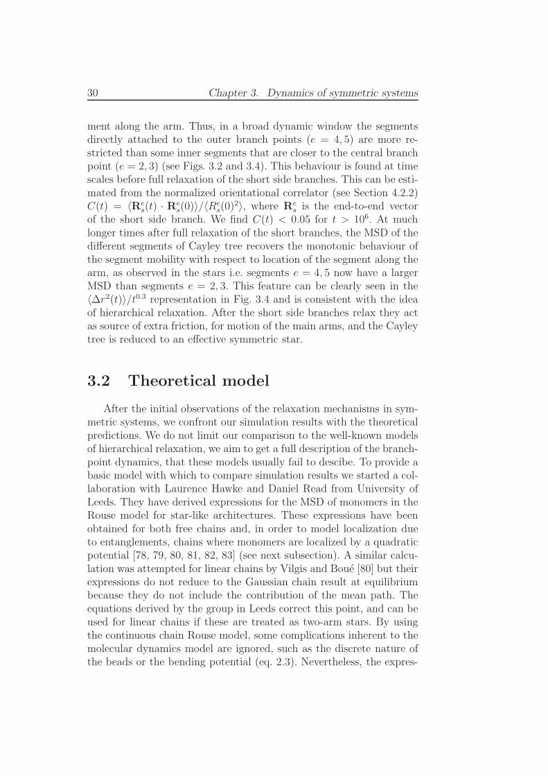
the derivations the reader is referred to the Appendix in [85]. We onlypresent the final expressions for MSD that are necessary for the furthercomparison of the theoretical model with simulation data.

The results are summarized in Table 3.2. The factor kb appearingin the expressions is equal to Ns/N

2e . The appropriate selection for kb,

according to Read et al. [83], is kb = 1/4.

Table 3.2: MSD for entangled stars, author Laurence Hawke [85]

MSD Expression

〈(rα,s,t − rα,s′,t′)2〉 a2|s− s′|+ a2

√kb

[exp

(−|s−s′|√

kb

)− (f−2)

fexp

(−(s+s′)√

kb

)]−

a2√kb

2

[2 cosh

(|s−s′|√

kb

)− ΩA

−(s, s′, te)− ΩA

+(s, s′, te)

]+

a2√kb

2(f−2)

f

[2 cosh[ (s+s′)√

kb]− ΩB

−(s, s′, te)− ΩB

+(s, s′, te)

]

〈(rα,s,t − rβ,s′,t′)2〉 a2(s+ s′) + 2a2

√kb

fexp

(−(s+s′)√

kb

)−

a2√kb

f

[2 cosh[ (s+s′)√

kb]− ΩB

−(s, s′, te)− ΩB

+(s, s′, te)

]

〈(rα,s,t − rα,s,t′)2〉 a2

√kbΦ

(√te

π√kb

)− a2

√kb

2(f−2)

fexp

(−2s√kb

)[1 + Φ

(√te

π√kb

− πs√te

)]+

a2√kb

2(f−2)

fexp

(2s√kb

)[1− Φ

(√teπ√kb

+ πs√te

)]

〈(rα,0,t − rα,0,t′

)2⟩ 2a2√kb

fΦ

(√te

π√kb

)

where Φ(x) = 2√π

∫ x

0e−u2

du

ΩA−(s, s

′, te) = exp

(−|s−s′|√

kb

)Φ

(√te

π√kb

− π|s−s′|2√

te

)

ΩA+(s, s

′, te) = exp

(|s−s′|√

kb

)Φ

(√te

π√kb

+ π|s−s′|2√

te

)

ΩB−(s, s

′, te) = exp

(−(s+s′)√

kb

)Φ

(√te

π√kb

− π(s+s′)

2√

te

)

ΩB+(s, s

′, te) = exp

((s+s′)√

kb

)Φ

(√te

π√kb

+ π(s+s′)

2√

te

)


At this point it must be reminded that it was assumed in the theo-retical model that motion is dominated by fast Rouse modes. Therefore,the expressions presented in Tables 3.1 and 3.2 are valid for timescalesmuch smaller than the Rouse time of the arm, τRa

, and for segmentsclose to the central branch point. Thus, in the next Section we willlimit the comparison between the theoretical MSD and the simulationresults to the case of the branch point, since it exhibits only a weakrelaxation within the MD window (see Figs. 3.1 to 3.4).

3.3 Quantitative evaluation of molecular

dynamics data

3.3.1 Simulations with fixed chain ends

As discussed in Section 3.1 (Figs. 3.1 to 3.4), in the MD simulationsof entangled stars and Cayley trees several relaxation modes are activeat different timescales. At early times t < τe the dynamics of the chainis dominated by Rouse motion. The Rouse regime is followed by localreptative motion (‘Rouse in tube’ dynamics) and by arm retraction de-pending on the position of the segment along the arm. Additionally, armretraction contributes continuously to constraint release [15]. Since thetheoretical expression for the segmental self-motion (〈(rα,s,t − rα,s,t′)

2〉of Table 3.2) accounts only for internal Rouse modes its validity shouldbe tested initially against MD simulations where all other relaxationmechanisms are to a high degree inactive. Accordingly, in the regimewhere such mechanisms are not effective we do not expect significantdifferences between the motion of the branch point in the simulatedstars and that of the central branch point in the Cayley trees. In theremainder of the chapter the data presented for the branch point mo-tion in the Cayley tree must be understood as that of the central branchpoint.

With these ideas in mind, we have performed additional MD sim-ulations of symmetric stars and Cayley trees in which the ends of thelong and short arms are fixed in space. This suppresses arm retraction,as well as constraint release driven by arm retraction, and therefore itprovides information that can be directly compared with the theoreticalresults of Section 3.2.2. The corresponding MSD with their error bars,obtained from MD with fixed ends, for segments close to the branchpoint are shown in Fig. 3.6 with open symbols. Specifically, open redcircles and open blue circles refer to the MSD of the branch point in

3.3. Quantitative evaluation of molecular dynamics data 37

the star and Cayley tree, respectively. In the same figure their averageMSD (up to time scales of t ∼ 106 for which data for both branchpoints exist) is also shown with small close triangles. For improvingstatistics, the MSD is averaged over ten monomers, namely the branchpoint and the three nearest monomers in each arm. We shall refer tothis group of ten monomers as ‘the branch point’ of the simulation. Asexpected, the results confirm that on the time scales relevant for ourcombined study there are no differences, within statistics, between theMSD of the branch point in the star and Cayley tree.

103 104 105 106 107

10

15

20

25

10-1 100 101 102 103 104 105 106

0.1

1

10

MSD

t

MD average MD Star fixed ends MD Cayley fixed ends without early tube dilation with early tube dilation alternative fit without early tube

dilation, 2=49, e=2000

2=38 e=1200

Figure 3.6: MD results for the MSD of the branch point of the symmet-ric star (open red circles) and of the central branch point of the Cayleytree (open blue circles) with their respective error bars. The close smalltriangles refer to the their average MSD up to t ∼ 106. The full grey linecorresponds to the theoretical MSD without including the early tubedilation process. The dashed grey line represents an attempt to describethe whole spectrum of the data with different set of parameters. Theblack line shows the theoretical prediction when early tube dilation istaken into account. The theoretical predictions (lines) were obtainedby using the expressions derived by Laurence Hawke (Table 3.2).

Fig. 3.6 also includes the theoretical prediction (author LaurenceHawke) as a full grey line. In a similar manner to the average performedin the MSD of the simulations, we have averaged over the MSD for thecontinuous chain between s = 0 and s = 3N−1

e for each arm. Thesame procedure is performed in the comparison with the case of freeends (see Fig. 3.13 and explanation below). The theoretical MSD hasbeen constructed by using the parameters a2 = 38 and τe = 1200. By


adjusting the parameters a2 and τe we can obtain agreement betweenthe predicted MSD and simulation data in the Rouse regime or/andin the apparent plateau region, but so-obtained MSD curves fail inthe description of the crossover between these two regimes at times2000 < t < 105. One example of such theoretical curve with a set ofparameters a2 = 49, τe = 2000 is shown in Fig. 3.6 with dashed greyline. Thus the values of a2 = 38 and τe = 1200 were forced in orderto match the theoretical and the simulation MSD in the Rouse andcrossover regime (compare symbols and full grey line in the inset ofFig. 3.6 in the interval 10 . t . 105). Obviously, since the theoreticalmodel predicts Rouse dynamics at t → 0, it does not account for theearly ballistic motion observed in MD (see timescales t < 10 in the insetof Fig. 3.6). The theoretical entanglement time τe = 1200 is somewhatsmaller than the value τe = 1800 estimated from previous simulationMSD [47]. Nevertheless, taking into account, that local stiffness effectsin the simulated chains are not implemented in the theoretical modeland that there are some uncertainties in the method of τe estimationfrom the simulation, these two values of entanglement time are in arelatively good agreement.

The most noticeable feature in Fig. 3.6 is that at times significantlybeyond τe (i.e. times greater than 104), the MD data continue to risewhilst the theoretical MSD forms a clear plateau. The plateau in thetheory is fully expected since no other relaxation mechanism, exceptinternal Rouse motion, is included [85]. In contrast, the MD data clearlyindicate that, even if the arm ends are fixed, branch points remain freeand it seems they can experience some relaxation of the entanglementconstraints. This relaxation occurs after the branch point has exploredits initial entanglement cage at the timescale τe.

A possible interpretation of this observation is that there is someprocess occurring after τe, giving rise to an apparent slow relaxation ofthe branchpoint localization. We refer to this process as a ‘tube dila-tion’, as it shares some features with the processes softening the tube.However, we should bear in mind, that this process is not a dilution in asense of widening of the tube due to ‘standard’ constraint release fromarm retraction and removal of entanglements of surrounding chains,because this relaxation mechanism is absent in this simulation. Indeedthe mean path cannot relax since the arm ends are fixed and progres-sive dilution of the entanglement network mediated by the retractionof the arms is not possible. We can only speculate as to the mecha-nisms involved in this early ‘tube dilation’ process. It could be due totension equilibration along the constraining chains, which might relax


some of the localizing potential and would occur at the Rouse time ofthe arms. In an earlier work Zhou and Larson [86] investigated, by MDof a similar bead-spring model, melts of linear chains with fixed chainends. They also reported tube dilation and attributed it to a new typeof constraint release (see Fig. 7 in Ref. [86]), called ‘end looping’ con-straint release (ELCR), which occurred through Rouse motion. ELCRin melts of linear chains has also been studied at the level of primitivepaths [21]. However, for strongly entangled chains this process is onlyeffective near the chain ends [86], and we do not expect it to be relevantfor relaxation of the branch point in the systems investigated here.

Figure 3.7: For a selected star in the simulations with fixed ends, tra-jectory of the branch point (orange dots) and mean paths of the threearms (black, blue and green). Perspective depth is used. A deep fluc-tuation of the branch point along the green arm is clearly observed.

An alternative possibility is that the branch point makes short ex-cursions along the tubes of each arm (‘diving modes’ [87]), which inentropic terms are not so unfavourable as end looping. A precise char-acterization of the microscopic mechanisms involved in the early tubedilation process is beyond the scope of this thesis. Still, it is worthmentioning that visual inspection of branch point trajectories, in theMD simulations with fixed ends, gives some indications of the divingmodes. Concretely, the branch point diving can be seen in roughly halfof the branch point trajectories of Cayley tree and symmetric stars.Fig. 3.7 shows an example for a selected star. Orange dots representthe trajectory of the branch point (plotted at intervals of t ∼ 0.1τe).The three curves formed by the black, blue and green lines are the


‘mean paths’ of the three arms. These have been obtained by averagingthe monomer positions over the whole trajectory of the simulation withfixed arms, and provide an estimation of the tube contour. The shapeof the trajectory in the figure is not spherical and reveals a deep explo-ration of one of the tubes (green arm) by the branch point. Such a deepwithdraw of the branch point in only one particular direction occursrarely, in the most cases the trajectory has an elliptical or triangularshape, indicating much milder branch point excursions in two or threearm tubes.

Irrespective of its origin, we wish to quantify the magnitude of thisapparent ‘tube dilation’ process. This is so that when we (later) con-sider simulations in which the arm ends are not fixed, and constraintrelease is active, we can consider the additional, and much stronger,rescaling of the tube diameter due to constraint release, assuming thatthis acts as an independent process. We assume that the tube enlarge-ment depends weakly on time so there is a separation of timescalebetween fast Rouse motion within the tube and a slower ’tube en-largement’ process. Therefore, the expression for 〈(rα,s,t − rα,s,t′)

2〉 inTable 3.2 may still be used after rescaling appropriately the modelparameters as

a2(∆t) =a2

g(∆t), τe(∆t) =

τeg2(∆t)

, s(∆t) = s0g(∆t) (3.7)

where ∆t = |t− t′|. Under this renormalisation the early Rouse-in-tubebehaviour remains unchanged. The term g(∆t) is a slowly varying tubedilation function which is obtained by minimising the error betweenthe theory and the averaged branch point MD data (i.e. the smallclose triangles of Fig. 3.6) using trial values in the range [0, 1]. Theso-obtained function g(∆t) can be fitted to

g(∆t) =

g0 + g1, if ∆t ≤ t0

g0 + g1 exp(− (∆t− t0)/τg

), if ∆t > t0

(3.8)

with g0 ≈ 0.75, g1 ≈ 0.25, τg ≈ 22600.0, and t0 = 5010.0 for bothstars and Cayley trees (since the respective MSD from simulations areidentical within statistics). The black line in Fig. 3.6 represents thetheoretical MSD of the branch point after incorporating the effect oftube dilation as described above. It is worth mentioning that g(∆t) atthe longest MD time approaches a value of 0.75, which can be inter-preted as an increase of the original tube diameter a of the order of


15%. The effective relaxation time τg for the tube dilation is about fivetimes smaller than the Rouse relaxation time of an arm.

Having analyzed the mean square displacement for the branch pointin the MD with fixed arm ends, we can move on to assess the effects ofconstraint release in the case of the free ends. We present our findingsin the following subsection.

3.3.2 Simulations with free chain ends

Now we turn our attention to simulations with free ends (i.e. the‘standard’ constraint release is now active). As aforementioned, it is wellestablished that relaxation in symmetric star-like architectures doesnot occur by reptation, but via activated contour length fluctuations(CLF), also referred to as arm retraction [15]. When these fluctuationsare deeper than an entanglement spacing the chain has to manoeuvrearound the entanglements in order to fluctuate. This process is associ-ated with an entropic penalty. As the CLF from the arm tip towardsthe branch point become deeper, the conformation that the chain hasto adopt becomes entropically more unfavorable. This leads to a verybroad distribution of relaxation times, as demonstrated in Figs. 3.1 to3.4. In particular, the separation of relaxation timescales along a stararm is exponential [15]. During arm retraction constraint release is alsooccurring. When chains escape from their original tubes (by arm re-traction), they induce constraint release events on other chains. Thus,the molecular strands of the arms that are still unrelaxed (entangled)after a waiting time t, are able to explore a wider tube than the origi-nal one. Because of the broad spectrum of relaxation times, this tubedilation process due to CR is typically modeled as an effective dilu-tion of the entanglement network (see section 4.3.2 of Ref. [15]). Thisapproach is referred to as the ‘dynamic dilution hypothesis’ [15]. Ourpresent simulations represent an opportunity to test this hypothesis.

For both studied systems the time τa taken for a complete retractionof the long arm (Z = 8) is not reached within the MD window. Thus, atthe upper limit (2×107) of the simulation time window there is an armfraction of ≈ 0.3 and ≈ 0.4 in the star and the Cayley tree, respectively,that is still unrelaxed (see below). We take this fact into considerationand assume that branch point dynamics is still governed by chain mo-tion within a localizing potential at the end of the MD. If we make useof the dynamic dilution hypothesis, and assume that constraint releaseprovides an additional rescaling of the tube diameter over and abovethe early tube dilation process discussed in subsection 3.3.1, we expect


that the model parameters can be renormalized in this case as

a2(∆t) =a2

g(∆t)ψαd(∆t),

τe(∆t) =τe

g(∆t)2ψ2αd(∆t),

s(∆t) = s0g(∆t)ψαd(∆t), (3.9)

where ψ(∆t) is the fraction of material that is still entangled (un-relaxed) after a waiting time (∆t). The exponent αd is the so-calleddilution exponent, often assumed to be 1 or 4/3. In our calculations wehave investigated both values of αd (see Fig. 3.13). The factor g(∆t) isthe function obtained in the previous section (eq. 3.8) describing theearly tube dilation process. The dilution function ψ(∆t) correspondsto the tube survival probability [15]. We can estimate it directly fromthe simulations as follows. Following the original work of Doi and Ed-wards [25], we formulate the tube survival probability in terms of thetangent correlation function and specify it for the case of a three-armsymmetric star:

ψℓ(t) = 〈uα,ℓ,0 · (Reα,t +B′Re

β,t + C ′Reγ,t)〉. (3.10)

In this equation uα,ℓ,0 = ∂rα,ℓ,0/∂ℓ represents the tangent vector at theℓth segment in the arm α at time 0. Re

α,t = rα,Na,t− rα,0,t is the end-to-end vector of the arm α at time t. The three indices α, β, γ ∈ 1, 2, 3are different and denote the three arms of the star. The numericalcoefficients B′ and C ′ provide the weight of the correlations betweenthe arm α and the other two arms β and γ.

Equations similar to eq 3.10 have been proposed [88, 89], but us-ing the mean path rather than the chain coordinates. The differencebetween these two approaches is that the mean path includes an aver-age over short-time internal modes of the chain. With suitably chosencoefficients B′ and C ′, eq. 3.10 does not decay due to local Rouse mo-tion of the chain within the tube, and so it is not necessary to use themean path. We demonstrate this by evaluating eq. 3.10 for unentangledthree-arm symmetric stars. To do so, the tangent vector uα,ℓ,0 and theend-to-end vectors Re

α,t, Reβ,t, R

eγ,t should be expressed in terms of the

Rouse modes [85]. Regarding the coefficients B′, C ′, we consider first


the case B′ = C ′ = −1/2 (‘half-correlation’). The final expression reads

ψℓ(t) =4b2

π

∑p

12p−1

×[cos

((2p−1)πsℓ

2

)sin

((2p−1)π

2

)exp

(−tRa

(2p−1)2

4

)],

(3.11)

where sℓ = ℓ/Na and tRa= t/τRa

. In Fig. 3.8 eq. 3.11 is plotted (solidlines) as a function of the normalized time tRa

for different values of sℓ.In the usual continuous approximation, the sum in the former equationextends from p = 1 to p = pmax → ∞. For the numerical calcula-tion performed by Laurence Hawke pmax = 1000 was used. Results forlarger pmax were indistinguishable from those of Fig. 3.8. The figuredemonstrates that, for inner sections of the chain, the ‘half-correlation’function starts to decay at around τRa

indicating that it is insensitive tohigher order Rouse modes. For sections of chain close to chain ends, theinitial decay is seen at a timescale set by the Rouse time of the (1-sℓ)section of the chain (i.e. by τRsℓ

= τmonN2a (1− sℓ)

2). Short lengthscaleRouse modes never lead to decay of the function. Therefore the useof chain coordinates instead of the mean path has no significant effecton our calculations. The same applies when tube dilation is present.This is because tube dilation will not affect the decay of ψℓ(t), as itsimply introduces a few more fast Rouse modes to average over. Thusthe dominant mechanism for relaxation of ψℓ(t) is tube escape.

We also considered the option B′ = C ′ = −1 (‘full-correlation’). Asseen from the dashed lines in Fig. 3.8, by including the full correlationsbetween the star arms, the obtained function ψℓ(t) exceeds the maxi-mum expected value, i.e., ψℓ(t) > 1.0 and gives undesirable peaks forsegments close to the branch point (sℓ = 0.15, 0.3). To avoid this effect,we take into consideration only the half correlation (B′ = C ′ = −1/2)when we calculate eq. 3.10, for entangled stars, using the simulationdata (see below). The final choice of the prefactors B′ and C ′ for par-ticular segments of the star and Cayley tree is illustrated in Fig. 4.5.Note that each arm of the Cayley tree is divided into three differentparts (outer segments, inner segments, short arm), so there are moreterms on the right side of eq. 3.10 (and more than two prefactors B′, C ′

are needed, see Fig. 4.5 b.)). For the Cayley tree and the star arm in-dices α, β, γ denote in this case different parts of the molecule (e.g. inFig. 4.5 b.), α refers to the inner arm, β and γ would refer to the twoother inner arms, with prefactors of −1/2 each, and a fourth symbol isrequired for the outer arm, with prefactor −1.


solid lines:

dashed lines:B ' = C ' = -12

B ' = C ' = -1

arm tip

branch point

0.001 0.01 0.1 1 100.0

0.2

0.4

0.6

0.8

1.0

1.2

tRΑ

ΨHtL

b2

Figure 3.8: Tangent correlation function (eq. 3.10) for unentangledstars. The solid lines refer to ‘half-correlation’ (i.e. B′ = C ′ = −1/2)while the dashed lines to ‘full-correlation’ (i.e. B′ = C ′ = −1). Dif-ferent colours correspond to different Rouse segments along the arm,sl = 0.15 (black), 0.3 (magenta), 0.5 (red), 0.7 (green), and 0.85 (blue).The figure was made by Laurence Hawke and was included in this thesiswith his permission.

We move on to the entangled systems. We calculated the tangentcorrelation function (eq. 3.10) by using the simulation data. Thus, thetangent vector in eq. 3.10 was approximated by the end-to-end vec-tor of an arm segment of length equal to ten monomeric units. Thissegment size was chosen as a compromise to both achieving good statis-tics and averaging fast monomer fluctuations (not captured within thecoarse-grained tube model). In Fig. 3.10 we show the time evolutionof the so-obtained correlation functions for different segments sℓ of thesymmetric stars and Cayley trees. It is clear that not all the functionsfully relax within the MD time window. In particular, inner segmentsremain, on average, confined in their tubes — e.g., for sℓ = 0.3 the tubesurvival probability barely drops to the value ψℓ(t)=0.8 at the end ofthe simulation. The tangent correlators ψℓ(t) were fitted to stretchedexponential (Kohlraus-William-Watts, KWW) functions:

ψℓ(t) = exp(−(t/τℓ)βK ) (3.12)

where βK is the stretching exponent and τℓ is the relaxation time ofthe ℓth-segment. The stretching exponent βK varies with ℓ and reachesthe lowest values for segments close to the arm ends. From the fitting


Figure 3.9: Schematic representation of the correlations used for thecorrelator ψℓ(t). Numbers labeling particular segments are the pref-actors B′ and C ′ used in equation 3.10 and red colour highlights thesegment ℓ on the arm/part α. Figure a.) and b.) show the correlationsof the outer and inner segments of the long arm of the Cayley tree.Figure c.) illustrates the correlations of the short arm segments of theCayley tree.

procedure we get a set of points [sℓ; τℓ], that provides us the informationabout the consecutive relaxation of the segments along the arms. Wecan use this information to construct functions Ξα,β,γ(t) that representthe fraction of unrelaxed material of the star arms or Cayley tree’sparts α, β, γ. The function is normalized so that Ξα,β,γ(0) = 1 (allthe material is unrelaxed at t = 0), and it decays with time in anexponential-like fashion, until all the material is relaxed, Ξα,β,γ(τNa

) =0.

The procedure for obtaining the function Ξα(t) is illustrated inFig. 3.11 for the case of the stars (obviously the function is identicalfor the three arms α, β, γ). There we show the coordinates sℓ versus therespective KWW times τℓ, obtained from fitting the tangent correlatorsψℓ(t) as described above. This gives us a ‘discrete’ representation of thetime elapsed for relaxing the fraction of the arm tube extending froms = 1 (arm tip) to s = sℓ. Likewise, the fraction from s = sℓ to s = 0(branch point) will be the fraction of unrelaxed tube at time t = τℓ. Byfitting the discrete set of points in Fig. 3.11 to some model function, wewill obtain the continuous functions Ξα,β,γ(t) describing the tube sur-vival probability of each arm α, β, γ. Two model functions have been


0

0.1

0.2

0.3

0.4

0.5

0.6

0.7

0.8

0.9

1

1.1

100 1000 10000 100000 1e+06 1e+07 1e+08

ψ l(t)

t

star sl=0.3star sl=0.5star sl=0.8

Cayley sl=0.3Cayley sl=0.5Cayley sl=0.8

fit Cayley sl=0.8fit star sl=0.8fit star sl=0.5

Figure 3.10: Tangent correlation functions for the segments of sym-metric star (squares) and Cayley tree (circles) with the fitting KWWfunctions.

0

0.1

0.2

0.3

0.4

0.5

0.6

0.7

0.8

0.9

1

1000 10000 100000 1e+06 1e+07

s l

τl

dataKWW fit, Ξα

exponential fit

Figure 3.11: Symbols: for the stars, KWW times of the tangent corre-lators ψℓ(t) versus the respective coordinates sℓ. Curves: fits to expo-nential (blue) and KWW behavior (green).

used in the fit, namely an exponential (blue curve in Fig. 3.11) anda KWW function (green line). The data show strong deviations frompure exponential behaviour and are much better described by a KWWfunction (βK ≈ 0.4). As aforementioned, in the star Ξα(t) is identicalfor the three arms. In the case of the Cayley tree, we have three setsof points [sℓ; τℓ] for each arm, since this consists of three parts: outer


segments, inner segments, and short side branch. Thus, we performedfits for the three sets of data to obtain their (non-identical) functionsΞα(t).

0

0.1

0.2

0.3

0.4

0.5

0.6

0.7

0.8

0.9

1

10 100 1000 10000 100000 1e+06 1e+07 1e+08 1e+09

tube

sur

vival

pro

babi

lity ψ

(t)

t

Symmetric starCayley tree

Figure 3.12: Tube survival probability of the symmetric star and theCayley tree, obtained from the simulations.

Then, having the full description of the time evolution of the re-laxation of the star arms and Cayley tree’s parts, there is just a smallstep from the functions Ξα(t),Ξβ(t),Ξγ(t) to the total tube survivalprobability ψ(t) of the star and Cayley tree. The total tube survivalprobability can be calculated as:

ψ(t) =ZαΞα + ZβΞβ + ZγΞγ

Zα + Zβ + Zγ(3.13)

where Zα is the number of entanglements per star arm or Cayley tree’spart α. The functions ψ(t) for the symmetric star and Cayley treeare shown in Fig. 3.12. Note that these model functions, constructedby following the fitting procedure described above, extend beyond theMD time window (t & 107), and fully decay at t ∼ 109 but we notethis is simply a possible extrapolation of the data. Nothing that followsdepends on this. At the end of the MD, the decay is ψ(t) ≈ 0.3 and0.4 for the star and Cayley tree, respectively. Interestingly, the fractionof unrelaxed material is larger in the star than in the Cayley tree upto time scales of t ≈ 7 × 106. Then the two curves ψ(t) cross eachother, and at longer times tube relaxation is much faster in the stars.The observed behavior seems consistent with an initially stronger tubedilution in the Cayley trees, being facilitated by the presence of the


weakly entangled side branches. Indeed these relax in a time scale ofabout t ≈ 106, i.e, roughly in the time window for which the starsshow a higher ψ(t). In hierarchical models, after their full relaxationthe side branches act as friction points, and the Cayley tree reduces to astar containing ‘fat beads’ originating from the relaxed side branches.This additional friction slows down the retraction of the long arms,and relaxation of the Cayley tree at long times becomes slower thanin the stars. This picture seems consistent with the trends observed inFig. 3.12.

Finally, we use the tube survival probability estimated from thesimulations (through eq. 3.13) to obtain the theoretical MSD of thebranch point. The latter, as predicted by 〈(rα,s,t−rα,s,t′)

2〉 of Table 3.2,and using the rescaling parameters of eq. 3.9, is represented in Fig. 3.13with solid cyan lines and solid magenta lines for αd =1 and αd = 4/3,respectively. In the same figure the simulation data with free ends aredepicted with open black circles together with their respective errorbars. Note that in the majority of cases the width of the error bar isof a similar size to the width of the black open circle. The top panelrefers to the symmetric star while the bottom panel to the Cayley tree.For comparison we include the data of the simulation with fixed ends(small red and small blue circles), previously presented in Fig. 3.6.Since constraint release is now active, the MSD of the branch point islarger than its counterpart in the MD with fixed ends (compare theopen black circles with the small close circles at timescales bigger thant ∼ 105). Moreover, in the time window 103 . t . 5 × 106 the branchpoint in the star is more localized than in the Cayley tree, since atthese timescales ψ(t) of the star is bigger than ψ(t) of the Cayley tree(see Fig. 3.12).

From Fig. 3.13 it is clear that the theoretical prediction agrees verywell with the MD data for the case αd = 1. The results demonstratethat one can use the tube survival probability, parameterised by ψ(t),to predict the effective dilution of the tube diameter, measured fromthe mean square displacement of the branch point. This observation isa strong confirmation of the ‘dynamic dilution’ hypothesis. It remainspossible that a higher value of the dilution exponent, such as 4/3, couldbe used, but this would require some form of partial tube dilation, as(for example) suggested by Watanabe et al. [40].


102 103 104 105 106 107

10

100

10-1 100 101 102 103 104 105 106

0.1

1

10

100

MSD

t

MD data free ends Theory d=1 Theory d=4/3 MD data fixed ends

888 Star

102 103 104 105 106 107

10

100

10-1 100 101 102 103 104 105 106

0.1

1

10

100

Cayley tree

MSD

t

MD data free ends Theory d=1 Theory d=4/3 MD data fixed ends

Figure 3.13: MSD of the branch point of the symmetric stars (top)and Cayley trees (bottom) with free ends. MD data are shown as openblack circles. Their error is also shown with black bars. The solid cyan(magenta) curve corresponds to the theoretical MSD (author LaurenceHawke) using αd = 1 (αd = 4/3) and accounts for CR events and theearly tube dilation process. For comparison we also include the MDdata for fixed arm ends (small close circles with their error bars).


4. Dynamics of asymmetric

systems

In this chapter we investigate the dynamic behaviour of asym-metric systems, in particular T-shaped asymmetric stars, Y-shapedstars, combs and mixtures of asymmetric stars with linear chains (seeFig. 2.3). We focus on the branchpoint diffusion and we use the sim-ulation data to resolve some open questions related to the relaxationmechanisms of the asymmetric architectures. Namely, we determinehopping parameters from simulation data and critically discuss specifictheoretical assumptions for branchpoint hopping.

4.1 Diffusion of the branchpoint: theoret-

ical background

Figure 4.1: Schematic representation of the relaxation mechanisms inasymmetric stars. Left: Retraction mechanism, red arrows indicate themovements of the star arms. Middle: Relaxed arm acting as a frictionbead. Right: Reptation of the ‘effective linear chain’.

After the relaxation of the short arms, they effectively act as sourcesof additional friction, i.e., as frictional ‘fat beads’ (see Fig. 4.1). Thebranchpoint at these time scales probes the space liberated by the re-moved constraints of the arm, and performs diffusive steps (hops) along

52 Chapter 4. Dynamics of asymmetric systems

the tube contour with a diffusivity given by:

D =p2a2

2τa(4.1)

where τa is the longest relaxation time of the arm and a is the tubediameter.

Consequently the backbone, which in the case of the asymmetricstars is formed by the two long arms, is able to reptate. The branchpoint motion at these time scales can be seen as a curvilinear diffu-sion along a tube of diameter a. The trajectory of the branch point isassumed to be a random walk,

〈r2〉 = |L|a, (4.2)

where 〈r2〉 is the mean square distance between the start and end pointsof the trajectory, and |L| is the length of the primitive path that isexplored by the branch point in this trajectory. A Gaussian distributionis assumed for the diffusion length L. Therefore, eq. 4.2 can be expressedas

〈r2〉 = 2a√2π〈L2〉

∫ ∞

0

L exp

( −L2

2〈L2〉

)dL, (4.3)

which leads to the relation:

〈r2〉 = a√

2〈L2〉/π. (4.4)

Since we have assumed a diffusive motion of the branch point along theprimitive path, we can relate 〈L2〉 and the diffusivity D as

〈L2〉 = 2Dt (4.5)

where the factor 2 results from the one-dimensional character of thecurvilinear diffusion. From eq. 4.4 and eq. 4.5 we find:

D =π

4a2

(〈r2〉t1/2

)2

. (4.6)

Eq. 4.6 provides a direct way of obtaining the diffusivity for the curvi-linear, reptative motion of the branchpoint. In the reptative regime themean squared displacement will scale as [25] 〈r2〉 ∝ t1/2. Therefore, byobtaining from the simulations the corresponding plateau value of theratio 〈r2〉/t1/2, the diffusivity can be easily calculated. We note herethat when dynamic tube dilution is included, there are different tube

4.1. Diffusion of the branchpoint: theoretical background 53

diameters that could be considered. There are a set of nested tubes,each of which is parameterised by its tube diameter, a. As written,eq. 4.6 gives the effective diffusion constant for the random motionof the branchpoint, when this motion is mapped onto the path forthe tube with diameter a. Thus a particular motion (giving rise to aplateau value of 〈r2〉/t1/2) can be construed either as rapid diffusionalong a tube path with a small tube diameter, or as slower motionalong a shorter tube path with a larger tube diameter.

The branchpoint is assumed to hop in the tube every time the shortarm relaxes. This branchpoint hopping may occur in the skinny (a0) orin the dilated (a) tube. In order to investigate both possible cases, wemodify eq. 4.1 in the way it was done in eq. 11 of Ref. [7]:

D =p2a4h2qτaa2

. (4.7)

The parameter ah denotes the tube diameter (a0 or a) in which thebranchpoint hopping takes place. In deriving eq. 4.7, Ref. [7] assumesthat the length ah sets both (i) the typical distance of the hops, and(ii) the tube contour along which the hops take place. This is thenconverted to an effective diffusion constant D, for motion mapped on tothe tube path set by tube diameter a. We note that, if eq. 4.6 and eq. 4.7are equated then the factor a2 cancels: the large scale motion given by〈r2〉/t1/2 will depend only on the tube diameter ah within which hopstake place. We equate eq. 4.6 and eq. 4.7 below if we assume thatbranchpoint friction dominates the motion. This is to be contrastedwith, for example, Frischknecht et al. [49], who (when considering hopsin a skinny tube) sometimes consider the length of the hop to be setby a0, but the path of the hop to be along the dilated tube contour.

Eq. 4.7 includes an additional factor q. The factor q is the numberof side arms attached to the main backbone (q = 1 for the stars, q = 2for the combs), and it is introduced for accounting for all frictionalcontributions from the relaxed q short arms. In the case ah = a andq = 1, eq. 4.7 reduces to the original eq. 4.1.

As mentioned in the Introduction, the hopping parameter p2 used inthe expression for the branchpoint diffusivity was experimentally foundto be considerably smaller than unity, reflecting a stronger drag fromrelaxed arms than expected. A possible explanation is that eq. 4.1 andeq. 4.7 overestimate the diffusivity by missing the friction contribu-tion from the chain itself. We attempt to correct this point by addingthe chain friction for the motion along the skinny tube, allowing for arescaling to the dilated tube in the manner of eq. 36 of Ref. [90]. The


corresponding equation for the diffusivity reads:

D =

(3π2τeZ

φαda20+

2qτaa2

p2a4h

)−1

, (4.8)

where Z is the number of entanglements along the backbone, a0 is theundilated tube diameter, τe is the entanglement time, and φαd repre-sents the fraction of material giving rise to slow constraints (see below).As discussed in detail in Ref. [90] (building on the earlier work of Viovyet. al [91]), the factor φαd in the first term on the right hand side ofeq. 4.8 arises because the ‘solvent’ (giving the dilated tube) is actuallyformed by slow moving entangled chains. The fastest mode for diffu-sion along the dilated tube is via chain motion along the skinny tube.Motion directly along the dilated tube requires many constraint releaseevents and is therefore much slower. The factor φαd is due to projectingchain motion along the skinny tube onto the shorter diluted tube path.

For the mixtures of asymmetric 883-stars (see Fig. 2.3) and linearchains, constraint release from the solvent (the short, linear chains) isa little faster, and we can refine equation 4.8 to allow for chain motionalong the dilated tube, mediated by this constraint release (see eq. 39of Ref. [90]):

D =

3π2τeZ

a20

[φαd +

(2

3π2ντe+

1

1− φαd

)−1]−1

+2τaa

2

p2a4h

−1

, (4.9)

where ν = cντ−1s is the constraint release rate from the linear chains in

the mixture, τs is their relaxation time and cν is the rate constant. Ineq. 4.9 we have dropped the factor q since for the 883-stars q = 1. Wenote that, in the limit of extremely fast constraint release (ν → ∞) thefriction for chain motion along the dilated tube becomes independent ofφαd. In practice, even for the mixtures with short linear chains, eq. 4.9gives only a small correction to eq. 4.8.

Again, we contrast eq. 4.8 and eq. 4.9 with the work of Frischknechtet al. [49]. When considering reptation of the backbone along the dilatedtube, they assumed that the only friction experienced by the backbonewas the monomeric (or “Rouse”) friction. This neglects the fact that,for chain motion along the dilated tube, constraint release events needto occur, and these give rise to drag on the chain. Here we consider twopossibilities: that the constraint release events are so slow, the fastestmotion available to the chain is along the skinny tube, but subject tomonomeric friction - this gives eq. 4.8. For the blends, we also considerincluding constraint release events approximated to be at a fixed rate -

4.2. Analysis of the simulation data 55

this gives eq. 4.9. The work of Frischknecht et al. corresponds to eq. 4.9in the limit ν → ∞. Thus, in using eq. 4.8 and eq. 4.9, together withhopping in a dilated tube, we are considering an option not used byFrischknecht et al., namely branchpoint hopping in the dilated tube,but backbone motion dominated by movement along the skinny tube.Finally, if we know the tube diameter and use the simulation value forthe reptation plateau in 〈r2〉/t1/2, we can obtain the hopping parameterp2 by combining eq. 4.6 with one of the eqs. 4.7, 4.8, 4.9.

The equations presented in this section establish a direct relationbetween p2 and several observables that can be directly measured fromthe simulation. We determine this information and use it for obtainingthe corresponding p2-values.

4.2 Analysis of the simulation data

4.2.1 Branchpoint displacement

The plateau value of 〈r2(t)〉/t1/2 for eq. 4.6 can be directly obtainedfrom the simulation data, by analyzing the time evolution of the meansquare displacement (MSD, 〈r2(t)〉) of the branchpoint. However, thisMSD has poor statistics because of the limited number of branchpointsin the simulation box. In order to improve statistics considerably, weused the same procedure as in the previous chapter (Section 3.3.1)and we averaged the MSD of the ‘branchpoint’ over ten beads: theactual branchpoint and the three nearest consecutive beads at each ofthe three arms stemming from the branchpoint. Fig. 4.2 shows the so-obtained values divided by t1/2, for the different investigated systems.At long time scales, beyond t ∼ 106− 107 depending on the system, allthe data exhibit a plateau, except for the case of the symmetric stars.This result suggests that asymmetric stars and combs relax in such timescales by reptation, with the MSD showing the well-known power-lawbehavior 〈r2(t)〉 ∝ t1/2 for reptating linear chains [25]. For symmetricstars relaxation is exclusively mediated by arm retraction. Hence noplateau in 〈r2(t)〉/t1/2 is expected to arise at time scales beyond thesimulation window.

In order to obtain a reliable value of the plateau for eq. 4.6, weaverage the simulation data of 〈r2(t)〉/t1/2 ∝ t0 for times t > 5 × 106,where the plateau is well resolved. The so-obtained values are indicatedas horizontal lines in Fig. 4.2, and are listed in Table 4.1.


0.5

0.01

0.1

102 103 104 105 106 107 108

<r2 >/

t0.5

t

888881882883

mix11mix21Y4212comb

Figure 4.2: Symbols: MSD of the branchpoint divided by t1/2, for allthe investigated systems. The solid lines for each data set represent theaverage value of 〈r2(t)〉/t1/2 over the long-time plateau.

4.2.2 Relaxation times

In this subsection we determine the longest relaxation time, τa, ofthe short arm. For this, we analyze its end-to-end correlation function.This is defined as:

C(t) =〈Re(t) ·Re(t0)〉

〈Re(t0)2〉, (4.10)

where Re(t),Re(t0) is the end-to-end vector of the short arm at timest and t0 respectively. When the correlation function decays to 0 theshort arm is fully relaxed. We show the correlation functions of all thesimulated systems in Fig. 4.3. For each system we computed the end-to-end correlator for 15 equispaced uncorrelated time origins t0. Eachdata set in Fig. 4.3 is the average over the corresponding 15 correlators.The error bars indicate, for each time t, the respective upper and lowervalue obtained in the 15 correlators. In order to describe accuratelythe decay of the end-to-end correlator and to get a reliable value ofτa, we fitted the simulation data of Fig. 4.3 to several empirical func-tions. The stretched exponential Kohlrausch-William-Watts (KWW)function, gK(t) ∝ exp(−(t/τK)

βK), where βK < 1 and τK are fit pa-rameters, seems adequate for describing the observed nonexponentialdecay of C(t). KWW fits provided a good description in most cases, butfailed for the 883-stars and for the two mixtures, which exhibit a morecomplex decay. An alternative choice is to fit data to a weighted sum


0.1

-0.2

0

0.2

0.4

0.6

0.8

1

101 102 103 104 105 106 107

C(t)

t

881882883

mix11mix21Y4212comb

Figure 4.3: End-to-end correlators of the short arms for the differentsimulated systems. Symbols with error bars are simulation data. Solidlines are fits to a weighted sum of exponentials (eq. 4.11). The dottedline indicates the upper level of noise.

of exponential functions. Excellent fits (lines in Fig. 4.3) were obtainedwith five exponentials:

f(t) =5∑

i=1

Bi exp(−t/τi), (4.11)

Even if the fitting function provides a very good description of ourdata, the strong noise in the final decay of the correlation functionmakes the estimation of τa rather tricky. However, it is evident thatthe error bars in Fig. 4.3 do not exceed the value C(t) = 0.1. Wedefine the longest relaxation time of the short arm τa as the time atwhich the obtained fitting function drops to C(τa) = 0.1. This valueof C(t) is rather small and at the same time, the noise at that leveldoes not influence significantly the estimated value of τa. The averagevalues of τa with corresponding errors for the simulated systems arelisted in Table 4.1. In order to quantify the error of our estimation ofτa, we fitted to eq. 4.11 the 15 correlators computed for the differenttime origins. For each correlator we obtained a relaxation time fromthe condition C(τa) = 0.1, and we calculated the standard deviation ofthe so-obtained 15 values of τa.

At this point it is worth studying the possible effect of the chosenmethod on the final value of p2, namely by discussing other suggestedapproaches for obtaining τa from the simulation data. There have been


0.5

1

1.5

2

2.5

3

3.5

102 103 104 105 106 107

<r2 i>

/<r2 88

8>

t

881882883

Y4212

Figure 4.4: Ratio of the MSD of the T/Y-shaped asymmetric stars tothe MSD of the reference symmetric stars as a function of time. Thearrows are placed at the short arm relaxation times τa obtained by ourmethod (see Table 4.1).

some attempts to determine the longest relaxation time of the shortarm, τa, from slip-link [55] and molecular dynamics simulations [47].In the slip-link simulations τa was defined as the time when the shortarm loses all its entanglements [55]. In the MD simulations [47] τa wasdetermined as the time at which the MSD of the branchpoint of theasymmetric stars deviates from the corresponding data of the sym-metric stars. This estimation is based on the assumption that, afterthe short arm relaxation, the branchpoint is allowed to take a randomhop along the confining tube. This change in the branchpoint dynam-ics leads to a change in the slope of the MSD. Zhou and Larson ob-served [47] that this change occurred at the time when the end-to-endcorrelation functions of the short arms decayed to C(t) ≈ 0.2. How-ever, there is no systematic method to find an accurate time, wherethe MSD curves for asymmetric and symmetric stars split up, so thevalues of τa estimated by the naked eye have a significant uncertainty(up to one time decade). Moreover, in order to obtain the τa for themixtures we would need a reference system consisting of a mixture ofsymmetric stars and linear chains. In Fig. 4.4 we show the results (ar-rows) obtained by our method (see above) together with MSD data ofthe branchpoint (〈r2i 〉) for different architectures. The latter are dividedby the branchpoint MSD of the reference symmetric stars (〈r2888〉). Inthis representation, deviations from the branchpoint motion of the ref-


erence symmetric stars are reflected by deviations above the horizontallevel 〈r2i 〉/〈r2888〉 = 1. By direct inspection of Fig. 4.4 it seems that theprecise point at which deviations arise is ill-defined (note the scatterin the data). Still, it is clear that the so-defined relaxation times aresystematically smaller than those estimated by our method (arrows).As stated in Ref. [47], the time at which the branchpoint MSD deviatesfrom that of the reference symmetric stars is in very good agreementwith the time at which the short arm correlation function decays toC(t) = 0.2. Obviously this corresponds to a shorter time scale thatthe relaxation time used by us, obtained as C(τa) = 0.1 (see above).Namely, the former is about a 50 % smaller than our correspondingvalue for τa, which affects significantly the final value of p2.

In the case of the mixtures of asymmetric stars and linear chains,p2 is obtained from eq. 4.9, which contains as additional parameterthe relaxation time τs of the short linear chains in the mixture. Weproceeded in a similar manner as for the short arms in the branchedpolymers, by analyzing the end-to-end correlator of the linear chains.However, the relaxation time of the linear chains is obtained in theusual way, as C(τs) = e−1, unlike the condition C(τa) = 0.1 used forthe longest relaxation time of the short arms. We find τs = 19000.

4.2.3 Tube diameter and tube survival probability

As mentioned in the Introduction, one of the open questions regard-ing branchpoint dynamics is whether hopping takes place in the skinny(undilated) or in the fat (dilated) tube. In this subsection we inves-tigate both cases and estimate from the simulation the correspondingvalues for the tube diameter. First we calculate the original skinny tubediameter, a0, in our bead-spring polymers as:

a20 = NPPe C∞l

20, (4.12)

where C∞ is the characteristic ratio, l0 is the average bond length(l0 = 0.97, Section 2.1), and NPP

e is the entanglement length estimatedby primitive path analysis. By analyzing the asymptotic behavior ofintramolecular distances between distant beads (see Fig. 2.5), we ob-tain C∞l

20 = 3.46 ± 0.10 for all systems. We use the value NPP

e = 23reported by Everaers et al. [72], which was obtained for a melt of bead-spring chains at the same density and temperature, and with identicalinteractions as those used in our work. By inserting the former valuesin eq. 4.12, we obtain a diameter a0 = 8.92± 0.13 for the skinny tube.


In order to quantify the diameter of the fat tube for each investi-gated system, we first need to analyze the corresponding tube survivalprobability ψ(t) [85]. The procedure for obtaining ψ(t) involves thecalculation of the tangent correlation functions of polymer segmentsplaced on the different parts (labelled α, β and γ) of the given archi-tecture (eq. 3.10). These provide information on the relaxation timesof the primitive path coordinates, which can be used to determine thetime dependence of the tube survival probability. The procedure forobtaining the ψ(t) from the simulation data has been introduced in theprevious chapter for the symmetric stars and Cayley trees. There aresome modifications regarding the prefactors B′ and C ′ of eq. 3.10 for thecase of some asymmetric architectures. We consider three possible val-ues of the coefficients B′ and C ′: 0 (no correlation), -1 (full correlation)or -1/2 (half correlation). In the case of the 3-arm symmetric stars twoneighboring arms contribute equally with a prefactor -1/2 to the corre-lation with the third arm (see Section 3.3.2 for the explanation). Theintroduction of the full correlation (B′ = C ′ = −1) leads to artificialpeaks in the correlation function of the segments close to the branchpoint (Fig. 3.8). Following this argument, we use B′ = C ′ = −1/2 forthe arms of the Y-shaped stars. However, the situation is a bit differentin the case of T-shaped stars, where there are two equally long armsand one short arm. The tangent correlator of each of the long armsis largely dominated by correlations with the segments of both longarms. Hence, we can omit the correlations with the short arm in thetangent correlators of the long arms, taking the corresponding coeffi-cient as zero. We treat the linear chains in the star/linear mixturesas 2-arm stars, and we use the same coefficients as in the case of theT-shaped stars (Fig. 4.5a). In the case of the comb we use a similarprocedure based on the decomposition of the molecule into symmet-ric and asymmetric regions. Fig. 4.5 shows a schematic representationof all the correlations and corresponding coefficients for the T-shapedstars and comb.

Now we proceed in the same manner as in the case of symmetricsystems. We calculate the tangent correlation function ψℓ accordingto 3.10. uα,ℓ,0 figuring in this equation represents the end-to-end vectorof finite segment ℓ of length of ten beads. Few examples of tangentcorrelation functions for selected segments of 882 and Y4212 stars arepresented in Fig. 4.6. The decay of ψℓ for every segment ℓ can bedescribed by the KWW function (eq. 3.12).

The relaxation times τℓ obtained from these KWW fits are plottedin Fig. 4.7 as a function of the coordinate sℓ = ℓ/Na along the arm. The


Figure 4.5: Schematic representation of the weight of the correlationsused for the tangent correlator: a) T -stars, b) and c) comb. Numberslabelling particular segments are the prefactors used in 3.10. The partα containing the ℓth segment in this equation is represented with redcolor.

0

0.2

0.4

0.6

0.8

1

102 103 104 105 106 107

ψ l(t)

t

882 sl=0.4882 sl=0.6882 sl=0.8

Y4212 sl=0.4Y4212 sl=0.6Y4212 sl=0.8fit 882 sl=0.8

fit Y4212 sl=0.8

Figure 4.6: Symbols: tangent correlation functions of three segmentssℓ = 0.4 (red), sℓ = 0.6 (green) and sℓ = 0.8 (blue) in the long arms ofthe 882 T-shaped (squares) and Y-shaped Y4212 (circles) asymmetricstars. Lines are two representative KWW fits.


0

0.2

0.4

0.6

0.8

1

102 103 104 105 106 107 108

s l

τl

data long armdata short arm

exponential fit long armKWW fit long arm, ΞαKWW fit short arm, Ξβ

ψ(t)

Figure 4.7: Illustration of the procedure for obtaining the tube survivalprobability in the 883-star. The data [sℓ; τℓ] for the long (red symbols)and short (green symbols) arms are fitted to KWW functions. Thedashed line represents a single exponential function. The final tubesurvival probability, calculated according to 3.13, is given by the blueline.

discrete set of data [sℓ, τℓ] for each arm can be described by an empiricalfunction, which allows us to assign, in a continuous way, a fraction ofunrelaxed arm to every time t. Stretched exponential functions Ξα,β,γ(t)are the best choice for the sought empirical function (see Fig 4.7). Con-tinuous functions Ξα,β,γ(t) correspond to the tube survival probabilityof each arm α,β,γ and are the basic elements of the expression for thetotal tube survival probability (eq. 3.13). In Fig. 4.8 we demonstratethe effect of the dilution caused by the linear chains on the relaxationof the star segments in the mixtures. The data [sℓ; τℓ] for the long andshort arms of the 883-stars in the mixtures decay faster than the datafor the pure 883-stars. As a consequence, the functions Ξα,β,γ(t) for thestar arms in the mixture contribute to the altered shape of the finaltube survival probability of the mixtures in comparison to the puremelts (see below).

The obtained results for the tube survival probabilities are repre-sented in Fig. 4.9. The dilated tube diameter at the relaxation time τaof the short arm can be obtained as [15, 31]:

a2 =a20

ψαd(τa)(4.13)


0

0.2

0.4

0.6

0.8

1

102 103 104 105 106 107 108

s l

τl

883 long arm883 short arm

mix11 long armmix11 short armmix21 long arm

mix21 short arm

Figure 4.8: The data [sℓ; τℓ] for the long (circles) and short (squares)arms of 883 star in pure melt and in mixtures. Similarly to Fig. 4.7,data for pure melt of 883 stars are fitted to KWW functions.

where ψ(τa) is the value of the tube survival probability at theaverage time τa (see above), and αd is the dilution exponent. In theanalysis of the hopping parameter p2 (see below) we will consider thetwo suggested values of the dilution exponent [31], αd = 1 and αd = 4/3.As we discussed in the previous subsection, for each simulated systemwe use a set of 15 end-to-end correlators (computed at distinct timeorigins), yielding their respective values of τa. Accordingly, we have acorresponding set of 15 values for ψ(τa). We use these for computingthe standard deviations of ψ(τa) (see below).

The calculated tube survival probability is directly related to theparameter φαd in eqs. 4.8-4.9 via:

φαd = ψαd(τa). (4.14)

This parameter represents the fraction of the material that is respon-sible for the slow constraints in the system. After the relaxation of thefastest parts in our systems (short arms, and linear chains in the mix-tures), the only slow components to relax are the long arms or mainbackbone. This information is contained in ψ(τa), which measures theunrelaxed tube fraction at τa, i.e., at the time scale of the relaxationof the short arm. This is also the case for the investigated star/linearmixtures. Indeed the relaxation time for the linear chains is, at most,that of the short arms, since both have the same length (three entan-glements, see Fig. 2.3), but the short arms have only one free end.


0

0.2

0.4

0.6

0.8

1

101 102 103 104 105 106 107 108

tube

sur

vival

pro

babi

lity Φ

(t)

t

881882883

mix11mix21Y4212comb

Figure 4.9: Tube survival probability obtained from the simulations forall the investigated systems.

Some general trends are inferred from simulation data in Fig. 4.9.The two mixtures exhibit an abrupt decay in the range 104 . t . 105.The beginning of this decay is consistent with the estimated relaxationtime of the linear chains (τs = 19000, see above). Thus, completionof the relaxation of the short linear chains leads to a sharp removalof constraints. As expected, the larger fraction of linear chains in themixture 1:1 produces a stronger decay of ψ(t) than in the mixture 2:1.Differences in the tube survival probabilities of the T-shaped stars (881,882, and 883) and the Y4212-stars are small at all time scales, whichsuggests a relatively small role of the relaxation of the short arms inthe total ψ(t) of these systems, and once the short arms are relaxed,a similar amount of constraints are removed by reptation. The tubesurvival probability of combs is markedly different from that of the T-and Y-stars. It shows a faster decay up to time scales of about τa. Thisis consistent with a stronger role of dynamic tube dilution in combs,due to their higher volume fraction of short arms than in the T- andY-stars. However, after relaxation of the short arms, the combs containtwo frictional fat beads close to the both ends of the linear backbone.This strongly hinders relaxation and ψ(t) exhibits a very slow decayover the following time decades, prior to the late decay by reptation.

The tube survival probabilities obtained from the simulations can bedirectly compared with theoretical predictions from hierarchical mod-els. Here we compare our results with those from the branch-on-branch(BoB) model developed by Das et al. (see Ref. [7] for details). The BoB


0

0.2

0.4

0.6

0.8

1

101 102 103 104 105 106 107 108

tube

sur

vival

pro

babi

lity Φ

(t)

t

Asymmetric star 882

Simulation dataBoB p2=1.0 α=4/3

BoB p2=1/60 α=1.0

0

0.2

0.4

0.6

0.8

1

101 102 103 104 105 106 107 108

tube

sur

vival

pro

babi

lity Φ

(t)

t

Mix asymmetric star(883):linear chain 1:1

Simulation dataBoB p2=1.0 α=4/3

BoB p2=1/60 α=1.0

Figure 4.10: Comparison between the tube survival probabilities ob-tained from the simulations (solid line) and from the BoB modelwith choice of parameters p2 = 1, αd = 4/3 (dashed line) and p2 =1/60, αd = 1 (dash-dot line).

model makes detailed predictions for linear rheological data of non-looped branched architectures of arbitrary complexity, by using theentanglement length and entanglement time as external inputs. Out-put of the BoB calculation includes the tube survival probability ψ(t).Fig. 4.10 compares BoB and simulation results of ψ(t) for some rep-resentative cases (882-stars and star/linear mixture 1:1). BoB assumesa priori values for αd and p2. The results in Fig. 4.10 are obtainedfor two limit cases p2 = 1/60, αd = 1 (dash-dot lines), and p2 = 1,αd = 4/3 (dashed lines). These include the two values used for the


scaling exponent αd and the lowest and highest value of p2 reportedin the literature [49]. Both the hopping parameter p2 and the scalingexponent (through the factor ψ−αd(τa)) determine the friction constantfor the final reptation of the system. Therefore, in systems where finalrelaxation is mediated by reptation, decreasing the values of p2 andαd moves the reptative regime to longer timescales. Thus, the casesp2 = 1/60, αd = 1 and p2 = 1, αd = 4/3 provide an upper and lowerbound for the onset of reptation predicted by BoB. Relaxation by rep-tation in the BoB curves of Fig. 4.10 corresponds to the final sharp dropto zero [7]. This time scale can change by even one decade accordingto the specific choice of p2 and αd.

Having noted this, the chosen values of p2 and αd do not signif-icantly affect the obtained BoB curves in the time window, t ≤ τarelevant for our estimations of p2 (relaxation before arm retraction isindependent of p2 and changing αd from 1 to 4/3 introduces less than0.1% difference in ψ(t) at τa for the molecules investigated). Indeed, weestimate p2 from the simulations by using information on ψ(t) at therelaxation time of the short arms τa (through equations for the diffu-sivity in Section 4.1 and 4.14), i.e., much before the onset of reptation.As shown in Fig. 4.10 the two limit cases of p2 and αd used to generatethe BoB curves lead to essentially the same results in the former timewindow, differences only arising at much longer times. Still, it must benoted that αd should have a significant effect in that window for longside arms. In the cases investigated here the effect is negligible becausethe side arms are weakly entangled and stay in the early fluctuationregime.

In general, the simulation results for the tube survival probabilityare in qualitative agreement with the corresponding BoB results. Theagreement is even semiquantitative in the case of the pure T-stars.The BoB model captures the trends observed by simulations, includingthe crossover between fast dynamics of the short linear chains/sidebranches and slow relaxation of the long backbone. Having said this,it must be noted that for some systems (Y4212-stars and combs) asignificant part of the final relaxation of the backbone occurs at timesbeyond the simulation window (t & 4× 107), so conclusions about thecomparison at such time scales must be taken with care.

Once the reptation plateau in 〈r2〉/t1/2, as well as τa and ψ(τa)have been determined from the simulations, we can directly obtain theactual value of p2 (see Section 4.3). According to the discussion in Sec-tion 4.1, different expressions will be used for p2. These will dependon the specific architectures and compositions (pure or mixture), as


104

105

106

107

881 882 883 Y4212 mix11 mix21 comb

τ a, τ aΦ

8/3

simulation data τaΦ8/3, α=4/3BoB results τaΦ8/3, α=4/3

simulation data τaBoB results τa

Figure 4.11: Comparison of the simulation results of τa and τaψ2αd(τa)

with BoB predictions for the dilution exponent αd = 4/3.

well as on the choice of hopping in the dilated or in the skinny tube.In the different expressions of p2, the values of τa and ψ(τa) will en-ter separately and/or through the product τaψ

2αd(τa) (see Section 4.3).Fig. 4.11 shows simulation results of τa and the product τaψ

2αd(τa),for the case of dilution exponent αd = 4/3, in comparison with thecorresponding results obtained from the BoB model. A good agree-ment is again found, with some tendency for overestimation by BoB.Similar agreement is observed for the case αd = 1. With all this, weconclude that our procedure provides a robust estimation of tube sur-vival probabilities and relaxation times of the short arms, allowing fora reliable estimation of the hopping parameter p2, as will be discussedin Section 4.3.

4.2.4 Branchpoint trajectories

A further test of consistency for the estimated arm relaxation timescan be obtained by analyzing the real-space trajectories of the branch-points. Hierarchical models postulate branchpoint diffusion after re-laxation of the short side arms. Prior to this, the branchpoint remainsstrongly localized. In order to test this hypothesis we have analyzed theshape of the trajectories at different time scales. Thus, for times t > 105

we have saved the coordinates of the branchpoint every τ = 2000 timeunits. This roughly corresponds to one entanglement time (τe = 1800).At earlier times we have used shorter intervals for saving the branch-


0.15

0.01

0.1

102 103 104 105 106 107

Asph

erici

ty A

t

random walk

888881882883

mix11mix21Y4212comb

Figure 4.12: Time dependence of the asphericity of the branchpoint tra-jectory for all the simulated systems. The horizontal line represents thelimit case of a random walk. The arrows indicate the relaxation timesτa of the short arms, as determined independently from the analysis oftheir end-to-end correlators (see text).

point positions. Namely we have used τ = 2×10n−2 for the time decade10n < t ≤ 10n+1, with 2 ≤ n ≤ 4. With this, we use a large numberof points (at least 50) to characterize the shape of the branchpointtrajectory at any relevant time. This characterization can be made bycomputing the asphericity parameter, defined as:

A =(I2 − I1)

2 + (I3 − I1)2 + (I3 − I2)

2

2(I1 + I2 + I3)2(4.15)

where I1, I2, I3 are the semiaxes of the inertia ellipsoid of the trajectory.Thus, at each selected time t, we compute the asphericity A(t) of the setof points consisting of the saved branchpoint positions at times t′ ≤ t.More precisely, for the time t we only use the points t′ ≤ t saved everyτ time units, with τ the interval for saving used in the time decadewhich t belongs to (see above). For example, for t = 4 × 103, we usethe branchpoint positions at t′ ≤ t saved every 20 time units. For anytime t > 105 we use those saved every 2000 time units. In this waywe get a fair characterization of the asphericity at any time, by alwaysanalyzing a set of points equispaced in time, and preventing ‘crowding’in the regions visited by the branchpoint during the early time decades.

Fig. 4.12 shows the time dependence of the asphericity of the branch-point trajectory for all the investigated systems. For comparison we

4.3. Calculation of the hopping parameter 69

include the value A ≈ 0.15 obtained for a particle performing a three-dimensional random walk. The evolution of the asphericity with timereveals interesting features. In the early stage of the simulation, theasphericity diminishes by increasing time. This means that new posi-tions of the branchpoint become localized in a limited region of thespace, forming a trajectory that becomes closer and closer to the idealspherical shape (A = 0). The asphericity reaches a minimum and thenincreases with time during the rest of the simulation, i.e., the branch-point trajectory becomes progressively unlocalized. The random-walklimit is not reached at the end of the simulation. This will happenat much longer time scales, in the three-dimensional isotropic diffusiveregime, 〈r2(t)〉 ∝ t. Note that for the asymmetric systems, only one-dimensional curvilinear diffusion (reptation), 〈r2(t)〉 ∝ t1/2, has beenreached within the simulation window.

The minimum in the asphericity seems to follow several trends.For the three investigated T-shaped stars, it becomes deeper, i.e., thebranchpoint becomes more localized, by increasing the length of theshort arm. As expected, the strongest localization is found for the sym-metric 888-stars. Localization in the 883-stars becomes weaker by mix-ing with short linear chains. In Fig. 4.12 we have indicated (arrows) therelaxation times τa of the short arms, as obtained by the method pre-sented in Section 4.2. Within statistical error, there is a clear correlationbetween these time scales and the beginning of the delocalization of thebranchpoint and later increase of the asphericity from the minimum.

4.3 Calculation of the hopping parameter

Now we use the information obtained from the analysis in Sec-tion 4.2 as input for obtaining the numerical values of p2 for each ofthe investigated systems. The values of the observables estimated fromsimulations — reptation plateau in MSD (〈r2〉/t1/2 ∼ t0) longest re-laxation time of the short arm (τa), and tube survival probability atthe time τa (ψ(τa)) — are summarized in Table 4.1. By inserting thesevalues, together with the tube diameter, into the equations presentedin Section 4.1, we can calculate the hopping parameter p2. If the back-bone friction is not considered, by combining eq. 4.6 and eq. 4.7 for thediffusivity we obtain:

p2 =qπτa2a4h

(〈r2〉t1/2

)2

. (4.16)


system 〈r2〉/t1/2 τa ψ(τa)881 0.066±0.003 37000±9000 0.849±0.011882 0.031±0.001 439000±65000 0.685±0.013883 0.023±0.001 2133000±507000 0.500±0.023

Y4212 0.036±0.001 349000±80000 0.678±0.009mix11 0.064±0.004 962000±265000 0.278±0.021mix21 0.045±0.002 1193000±221000 0.373±0.014comb 0.036±0.002 401000±57000 0.593±0.010

Table 4.1: Summary of the variables obtained from the simulations:reptation plateau in MSD (〈r2〉/t1/2 ∼ t0), longest relaxation time ofthe short arm (τa), and tube survival probability at the time τa (ψ(τa)).

In this equation we use a4h = a40 if hopping is assumed to occur inthe skinny undilated tube. In the case of hopping in the dilated tube,according to eq. 4.13 we use a4h = a40/ψ

2αd(τa).If we consider the backbone friction, then we make use of eq. 4.8

for the pure branched systems and eq. 4.9 for the star/linear mixtures.By combining each of these cases with eq. 4.6 we obtain the generalexpression for the hopping parameter:

p2 =2qa40πτaa4h

[(〈r2〉/t1/2)2

4a40 − 3π3τeZQ(〈r2〉/t1/2)2]. (4.17)

Again, a4h = a40 or a4h = a40/ψ

2αd(τa) if hopping takes place in the skinnyor dilated tube, respectively. The number of entanglements along thebackbone is Z = 16 for all the simulated systems (see Fig. 2.3). Thenumber of side arms is q = 1 in star-like structures and q = 2 in thecase of combs. The factorQ is equal to 1 in the case of the pure systems,whereas for the mixtures it stands for:

Q = ψαd2τs(1− ψαd) + 3π2cντe

2τsψαd(1− ψαd) + 3π2cντe. (4.18)

We assume a constraint-release rate constant [90] cν = 0.1 in the twoinvestigated mixtures of T-stars and short linear chains.

The reciprocal values of the hopping parameter 1/p2 for the simu-lated systems, calculated by using eq. 4.16 (no backbone friction) andeq. 4.17 (including backbone friction) are summarized in Table 4.2 andTable 4.3 respectively, for both dilution exponents αd = 1 and 4/3. Inboth Tables we just give the minimum and maximum possible values


αd 1 4/3 1 4/31/p2 ah = a0 ah = a0 ah = a ah = a881 17-38 17-38 25-51 28-56882 7-13 7-13 16-27 21-35883 3-5 3-5 11-20 18-30

Y4212 6-13 6-13 14-28 19-36mix11 1-2 1-2 10-19 25-42mix21 1-2 1-2 9-16 19-31comb 3-5 3-5 9-15 12-20

Table 4.2: Results of the calculation of 1/p2 in the simulated systemswithout considering additional friction of the backbone (i.e., by usingeq. 4.16). First column: simulated systems. Second to fourth columns:values of 1/p2. In the first two lines we indicate the used values of thedilution exponent (αd = 1 or 4/3), and whether hopping occurs in theskinny tube (ah = a0) or in the dilated one (ah = a).

of p2 in each system. For getting these values, we have made the cor-responding combinations of the upper and lower values (given by theirrespective error bars, see Section 4.2) of the parameters entering inthe former equations for p2, and have selected the minimum and max-imum output of such equations. This allows us to estimate p2 withinan uncertainty of typically about a factor 2.

The values of 1/p2 calculated from the simulation results are plottedin Fig. 4.13. There is a big gap between the values obtained by assuminghopping in the skinny or in the dilated tube. The gap in the 1/p2-valuesis indeed proportional to the factor 1/ψ2αd(τa) arising from assuminga4h = a40 or a4h = a40/ψ

2αd(τa) in eq. 4.16 and eq. 4.17. The effect ofthe tube widening on the former gap is, therefore, more pronounced inthe systems where a significant part of the molecule has been relaxedat the time τa. One clear example is the mixture 1:1. In this system,and for dilution exponent αd = 1, the value of 1/p2 for hopping in thedilated tube is about 10 times bigger than the corresponding value forhopping in the skinny tube.

The question of the apparent high friction exerted by the slightlyentangled short arms seems to be rationalized if one accounts for theeffect of the backbone friction on the branchpoint diffusivity. This effectis nicely illustrated in the case of the 881-stars, where the short armis only one entanglement long, and therefore the contribution of thebackbone friction is expected to play a relevant role in the diffusion of


αd 1 4/3 1 4/31/p2 ah = a0 ah = a0 ah = a ah = a881 8-23 8-23 11-30 13-34882 7-12 7-12 14-25 19-32883 2-5 2-5 11-19 17-29

Y4212 5-12 5-12 12-25 16-32mix11 1-2 1-2 9-18 25-41mix21 1-2 1-2 9-16 18-30comb 2-5 2-5 7-13 10-18

Table 4.3: As in Table 4.2, but considering the additional friction ofthe backbone (i.e., by using eq. 4.17).

1

10

100

881 882 883 Y4212 mix11 mix21 comb

1/p2

data without backbone friction, skinny tube, α=1data without backbone friction, dilated tube, α=1

data with backbone friction, skinny tube, α=1data with backbone friction, dilated tube, α=1

Figure 4.13: Representation of the results of Table 4.2 and Table 4.3for αd = 1. Symbols are the averages of the respective upper and lowervalues of 1/p2.

the branchpoint along the tube. For the case of αd = 1 and hopping inthe dilated tube, the value of 1/p2 for the 881-stars without includingthe backbone friction is about 40. If we include the backbone frictionin the diffusion constant the value of 1/p2 is lowered to approximately20, which is much closer to the respective values obtained for the othersystems.

We now restate our criterion, presented in the Introduction, for whatconstitutes a good set of assumptions about branch-point hopping: agood set of assumptions should result in broadly similar values of p2

across the different systems studied. By inspection of Tables 4.2 and 4.3


and Fig. 4.13, we conclude that a comparatively low dispersion in thevalues of 1/p2 is found only if the backbone friction is included in thediffusivity and hopping is assumed to occur in the dilated tube. Thisset of assumptions leads to roughly a factor 2 variation in the valueof 1/p2 across the systems studied, which is within the error boundsof our analysis. As is emphasized by the logarithmic axis in Fig. 4.13,results for other combinations of specific assumptions for branchpointhopping are very disperse, suggesting that they are inconsistent and canbe ruled out in models. For example, setting the length scale associatedwith the hops to the bare (skinny) tube diameter leads to a very widerange of the p2 values for different branched structures (variation bya factor of 10, which is significantly beyond the error bounds of ouranalysis).

With the assumptions of both inclusion of backbone friction andhopping in the dilated tube, the mean values of 1/p2 (defined for eachsystem as the mean of the upper and lower bound) fluctuate between10 and 20.5 if we use the dilution exponent αd = 1, and between 14 and33 if we use αd = 4/3. Thus, the diffusion of the branch point in thedilated tube with incorporated backbone friction points to an univer-sal behavior described in many experimental studies with parameter1/p2 = 12 [92, 32, 51].

Finally it is worth mentioning that our results for p2 are consistentwith these obtained (within the assumption of hopping in the dilatedtube) from linear rheology data of multiarm comb polymers (backbonefriction is not relevant here). The experimental analysis is part of thethesis of Helen Lentzakis (FORTH, Crete) and has been presented, asa collaborative work, in Ref. [19].


5. Real-Space Analysis of

Branchpoint Motion

In this chapter we inspect the branchpoint motion by performinga, purely geometrical, density-based cluster analysis of the branchpointtrajectories. We include in our analysis all branchpoints of the systemsthat reach the reptation regime within the simulation time window.Namely: the asymmetric stars 881 and 882, Y-shaped asymmetric starsY2214 and Y4212, mixtures mix11 and mix21, H-polymer and comb(more details about the architectures can be found in Fig. 2.3). Wealso analyze the trajectories of the outer branchpoints of the Cayleytree and the central bead of the linear chain. We identify regions ofstrong localization (‘traps’) in the trajectories and provide evidence ofbranchpoint diffusion between these traps. We present a density-basedmethod for the analysis of clusters (traps). This purely geometricalmethod allows us to compute time and length scales related to thebranchpoint diffusion along the tube from the simulation data, withoutinvoking tube-based model assumptions.

5.1 Heterogeneous branchpoint dynamics

First we examine heterogeneous dynamics and deviations from Gaus-sian behavior of the branchpoint motion. The main panel of Fig. 5.1shows the normalized van Hove self-correlation function, 4πr2Gs(r, t),of the branchpoint at a fixed time close to the end of the simulation(t = 2×107). The inset shows the time-dependence of the non-Gaussianparameter, α2(t) = 3〈∆r4(t)〉/5〈∆r2(t)〉2 − 1 (this becomes zero in thelimit of Gaussian behavior), where ∆r(t) is the displacement of thebranchpoint at time t. To improve statistics, the former functions havebeen averaged over ten monomers, namely the branchpoint and thethree nearest monomers in each of the three arms stemming from thebranchpoint. In the case of the linear chain the average was performed

76 Chapter 5. Real-Space Analysis of Branchpoint Motion

over seven beads, i.e. the central bead and the three nearest beads atboth sides of the chain. Though, within statistics, the non-Gaussianparameter seems to increase at times t > 103, this remains well belowunity at the end of the simulation time window. This finding is ratherdifferent from the behavior α2(t) > 1 observed in strongly heteroge-neous dynamic regimes, as e.g., the decaging regime in the vicinity ofa glass transition [93]. The low values found for the non-Gaussian pa-rameter of the branchpoints are consistent with the smooth shape ofthe van Hove functions, which do not exhibit neither secondary peaksnor long tails. These are also absent at other time scales within thesimulation window.

0

0.01

0.02

0.03

0.04

0.05

0.06

0.07

0.08

0.09

10 20 30 40 50

4πr2 G

s(r,

t)

r

881882

mix11mix21Y2214Y4212Cayley

Hcomblinear

0

0.2

0.4

0.6

10-1 100 101 102 103 104 105 106 107

α 2(t

)

t

Figure 5.1: Normalized van Hove self-correlations functions for thebranchpoints in the investigated systems, at the time t = 2×107 close tothe end of the simulation. Inset: time-dependence of the non-Gaussianparameter of the branchpoints. Data sets for the same system are plot-ted with identical colors in the main panel and inset (see legend).

The former features suggest that there is not a well-defined, sin-gle length and/or time scale for branchpoint hopping (which otherwisewould lead to a secondary peak in the van Hove function). Still, vi-sual inspection of typical branchpoint trajectories gives evidence ofstrong localization of the branchpoint in certain regions of the space(‘traps’). The left frame (grey points) of Fig. 5.2 shows a representative

5.2. Density-based cluster approach 77

‘smoothed’ trajectory of the branchpoint in the H-polymer. Smoothedtrajectories are obtained as follows. In all of the simulated systems thebranchpoints are regularly saved at every time interval of ∆t = 200.Then each consecutive block of 10 positions is replaced by its aver-aged position rav. The latter represents the average over a time inter-val ∆t = 2000, which corresponds approximately to the entanglementtime (τe = 1800) [47]. The smoothed trajectory is constructed by tak-ing all the averaged positions rav, i.e, it represents the branchpointtrajectory averaged over the local, fast Rouse-like vibrations occurringwithin the entanglement time. In the case of the linear chain the tra-jectory of the central bead is a set of its coordinates saved every timeinterval ∆t = 10000, i.e ∆t = 5τe. The total number of positions in thesmoothed trajectory is of the order of 104 which, as mentioned above,covers a simulation time scale of t ∼ 2× 107.

As can be seen in the figure, the trajectory reflects the motion ofthe branchpoint over a collection of traps. This is consistent with earlyresults by Zhou and Larson [47] for asymmetric stars in a shorter timewindow. There is not a clear separation between different traps, whichmakes the analysis of the data extremely complicated. Moreover, wefind that the character of the traps (dense or diffuse) and the shapeof the trajectories change significantly between different systems andeven within the same system. No quantitative characterization of thetraps was provided in Ref. [47]. In next sections we present a robust,purely geometrical method for such a characterization.

5.2 Density-based cluster approach

Despite the fact that different traps are separated by ill-defined,diffuse interfaces, it is still possible to identify the centers of the traps.The problem of detecting clusters of points in large databases arises inmany applications, e.g. minefield detection [94]. We solved this prob-lem by using an algorithm based on the approach of Xu et al. [95]. Theunderlying idea of this procedure is to find regions of very high densityof branchpoint positions, i.e, the regions in the trajectory that are morefrequently visited by the branchpoint. Branchpoint performs vibrationsaround the center of the trap, and occasionally jumps to another trap,where it is localized until it comes back to the original trap or movesto a new one. These wide vibrations and jumps lead to the diffuse, ill-defined interfaces separating the traps. The density-based cluster anal-ysis identifies clusters of branchpoint positions at high-density regions


Figure 5.2: Illustration of the procedure for identification of the local-ization traps. Left frame: representative smoothed trajectory (see text)of the branchpoint of an H-polymer. Middle frame: the same trajec-tory after dividing the points into cells with different density of pointsρp, and removing the low-density cells. Different intervals of density arerepresented with different colors. Yellow: 1 ≤ ρp < 3; green: 3 ≤ ρp < 4;cyan: 4 ≤ ρp < 6; blue: 6 ≤ ρp < 8; red: ρp ≥ 8. The red points corre-spond to cells of density equal to or above the threshold value ρth = 8,and are used to construct the clusters (right frame) representing thecenters of the localization traps. The same representation scale is usedin the three panels.

of the trajectory, and removes the irrelevant low-density interfacial re-gions.

We performed the density-based cluster analysis of each trajectory.For every point in the trajectory we calculate the distance rnn to itsnearest neighbor point in the same trajectory. Then we construct a 3d-grid with bin size, rb, identical to the maximum of all the rnn-valuesobtained within the trajectory. Even for trajectories of the same system,the set of rnn-values, and therefore also the value rb of the bin size, willdepend on each specific trajectory. The distribution of the rb values forall simulated systems is plotted in Fig. 5.3. The specific value of the binsize rb represents the size of the largest ‘hole’ that can be found withinthe considered trajectory. Thus, the whole trajectory can be mapped toa set of cells filled by points representing the branchpoint positions, andthe empty cells do not form part of the trajectory. This is consistentwith the fact that the maxima of the distributions of the rb values inFig. 5.3, for all the simulated systems, are placed at a distance a bitlonger than the average absolute value of the branchpoint displacement

5.2. Density-based cluster approach 79

2 2.5 3 3.5 4 4.5 5rb

0

0.25

0.5

0.75

1

1.25di

strib

utio

n881882mix11mix21Y2214Y4212CayleyHcomb

Figure 5.3: Distribution of the grid size rb for the simulated systems.

at the entanglement time (|r(τe)| ≈ 2.1 for the H-polymer, |r(τe)| ≈ 1.9for the 881-star).

Each point of the trajectory is assigned to the cell of the 3d-gridthat contains its position. For each cell, of volume r3b, in the 3d-grid ofa given trajectory, we define the local density of points, ρp = npr

−3b ,

with np the number of trajectory points within the cell. We find thatthe local density of points is not homogeneously distributed along thetrajectory. There are regions dominated by high-density cells separatedby regions of low-density cells, the first ones corresponding to the coresof the traps. This feature is illustrated in the middle frame of Fig. 5.2,which shows, for the same trajectory of the left frame and in the samerepresentation scale, branchpoint positions belonging to cells with den-sity ρp ≥ 1. Different colors correspond to different ranges of densityof the cells (see caption). The red points are located in the most densecells, with ρp ≥ 8. The middle frame of Fig. 5.2, by removing points inthe low-density cells (ρp < 1) that are visited by fast large-amplitudevibrations, nicely illustrates the formation of localization traps. It alsodemonstrates that points in the cells of high density are not randomlydistributed over the trajectory, but are organized into clusters.

We use the highest-density clusters to identify the centers of the


traps. First we fix a threshold density value ρth for all the branchpointtrajectories of a given system. Points in cells with local density ρp < ρthare discarded for the cluster analysis. To select the threshold value ρthwe first determine, for each cell in each trajectory, the integer partof the local density ρ

(int)p = int(ρp). Second, we determine for each

trajectory the maximum value of the former integer local densities,ρ(i,max)p = maxρ(int)p . The obtained value of ρ

(i,max)p , which is integer

by construction, will be degenerate, i.e, there will be several cells in thetrajectory with density ρp ≥ ρ

(i,max)p . In order to warrant the selection

of points for all the trajectories in the system, we define the thresholdvalue ρth as the minimum of the ρ

(i,max)p -values obtained for the different

trajectories. Finally, for each trajectory we select all the branchpointpositions located at the cells with density ρp ≥ ρth. We define thecentral regions of the traps as the clusters of such selected positions.Two of these selected positions in the same trajectory are assigned tothe same cluster if they are at mutual distance r ≤ rb/2, i.e., not largerthan half the bin size of the 3d-grid of the trajectory. Likewise, twoclusters merge into a single cluster if some point of one of the twoclusters is at a distance r ≤ rb/2 from some other point of the othercluster. The right frame of Fig. 5.2 shows the high-density clusters (ρp ≥ρth), obtained by the former procedure, that correspond to the fulltrajectory of the left frame. The density-based cluster analysis provideswell-defined separated trap centers for branchpoint localization.

5.3 Analysis of the time and length scales

Once we have indentified the high-density clusters in every trajec-tory of the simulated systems, we analyze the motion between traps.We consider that a point of a given trajectory is in a trap if it belongsto one of the high-density clusters (i.e., ρp ≥ ρth) defined above. If itis not the case, we consider that it belongs to one of the ‘transient’intervals corresponding to the diffuse interfaces separating the traps.In this way each trajectory can be mapped to a time-dependent dis-continuous function K(t), where 1 ≤ K ≤ nt is an index denoting eachof the nt traps in the trajectory, and t a discrete time variable denotingthe saved points of the trajectory (see above). If the time t belongs toone of the transient intervals, K(t) = 0. In Fig. 5.4 one simple case ofthe branchpoint motion between three traps is schematically depicted.In this scheme, the branchpoint is placed at time t1 in the first trap(K(t1) = 1), at time t2 it moves to the second trap (K(t2) = 2), at

5.3. Analysis of the time and length scales 81

Figure 5.4: Scheme of the motion of the branchpoint between traps. Thegrey arrows indicate the distance between the centers-of-mass of thetraps. The red dashed line with the red circle illustrates the fluctuationof the branchpoint out of the trap.

time t3 it escapes from the second trap (K(t3) = 0), and finally at timet4 it is placed in the third trap (K(t4) = 3).

Fig. 5.5 represents a typical realization of K(t) for the H-polymer.Only data withK(t) > 0 are shown, i.e., the transient intervals (K(t) =0) appear as blank spaces blinking between the intervals in the traps(blue symbols). During a transient interval the branchpoint makes ex-cursions out of the current trap, finally coming back to the same trap ormoving to another one. We define a transient interval [ti, tj ], of durationτt = tj−ti, in the discrete time sequence of a branchpoint trajectory, asthat obeying the conditions: i) K(t) = 0 for ti ≤ t ≤ tj , ii) K(ti−1) 6= 0,and iii) K(tj+1 6= 0). We define a residence interval of a branchpoint ina given trap k as an interval [t0, tf ], of duration τr = tf − t0, with theconditions: i) K(t0) = K(tf) = k, ii) K(t) = k or 0 for t0 < t < tf , iii)K(t′) 6= k at the largest t′ < t0 for which K(t′) 6= 0, and iv) K(t′′) 6= kat the smallest t′′ > tf for which K(t′′) 6= 0. Therefore, two times ti, tjfor which the branchpoint is in the same trap k belong to differentresidence intervals if there is, at least, one time ti < t < tj at whichthe branchpoint visits another trap k′ 6= k. Otherwise (K(t) = k or 0for ti < t < tj), they will belong to the same residence interval.


5.0×106

1.0×107

1.5×107

2.0×107

2.5×107

3.0×107

1

2

3

4

1.00×107

1.08×107

2

1.027×107

1.030×107

2

t

K(t

)

0

(b)

(c)

t

t

K(t

) K(t

)

(a)

Figure 5.5: Time evolution of the trap index K(t) for a typical branch-point trajectory of the H-polymer with four different traps. Symbolsfor K(t) = 0 are not shown. Thus, transient intervals appear as blankspaces blinking within or between residence intervals. Dotted lines areguides for the eyes. The red double-arrows indicate two residence inter-vals in the trap K=4, separated by a visit to the trap K=1. Main panel(a): whole trajectory. Insets (b) and (c): selected intervals, as indicatedby squares with arrows. The symbol size in the inset (c) corresponds tothe time resolution of the trajectory ∆t = 2000. To facilitate visualiza-tion, symbols sizes in (a) and (b) are bigger than ∆t, so they frequentlyhide short transient intervals, as illustrated by passing from (a) to (b)and from (b) to (c).

Fig. 5.6 shows the distributions p(τ) of transient and residence timesfor all the simulated systems. We find extremely broad distributions,that can be approximated by power laws, p(τ) ∼ τ−2.2 and τ−1 forthe transient and residence times respectively. We estimate the averagetransient time as 〈τt〉 =

∫τtp(τt)dτt/

∫p(τt)dτt, finding values, for all

the simulated systems, of the order of 〈τt〉 ∼ 104, i.e, about 5 entan-glement times. The distribution of transient times shows a much fasterdecay than the distribution of residence times. This indicates that mostof the transient intervals correspond to fast explorations of the inter-facial regions, before coming back to the original trap or moving to


103

104

105

106

107

τ10

-14

10-12

10-10

10-8

10-6

10-4

p(τ r),

p(τ t)

τ−2.2

τ−1

881882mix11mix21Y2214Y4212CayleyHcomblinear

Figure 5.6: Distributions of residence times (circles) and transient times(triangles). Circles and triangles with identical colors correspond to thesame simulated system (see caption). The lines indicate approximatepower-law behavior (exponents are indicated). The black double-arrowindicate the range of values obtained for the average transient time.The green double-arrow indicates the approximate range for the onsetof the apparent reptative regime in the MSD of the branchpoint (seebelow).

another one. Long explorations are very unfrequent events. Unfortu-nately we cannot estimate, in a similar manner, an average residencetime, 〈τr〉, from the data in Fig. 5.6. Whereas the long-time contribu-tion of p(τt) is already negligible at the end of the simulation window,in the former integrals for computing 〈τt〉, it is not the case for p(τr).Indeed, the observed power-law p(τr) ∼ τ−1

r cannot be extrapolated toarbitrarily long times since this would lead to divergent values of 〈τr〉.A correct estimation of 〈τr〉 would require the knowledge of p(τr) be-yond the simulation window. Still, by integration over the simulationwindow, we can determine a lower bound for 〈τr〉 of the order of 5×106.

Though the common scaling p(τr) ∼ τ−1r is evident, the overlap

of all the distributions p(τr) is an artifact of the used normalization∫p(τr)dτr = 1, where the integral is limited to the simulation window.

The scaling p(τr) ∼ τ−1r will break down (changing to a steeper be-


system ρth τa Φ(τa) a(αd = 1) a(αd = 4/3)881 8 37000± 9000 0.849± 0.011 9.68± 0.20 9.95± 0.23882 17 439000± 65000 0.685± 0.013 10.78± 0.26 11.48± 0.31

mix11 6 962000± 265000 0.278± 0.021 16.96± 0.89 21.02± 1.37mix21 10 1193000± 221000 0.373± 0.014 14.62± 0.49 17.23± 0.69Y2214 10 308000± 56000 0.692± 0.013 10.73± 0.26 11.41± 0.31Y4212 15 349000± 80000 0.678± 0.009 10.83± 0.23 11.56± 0.27Cayley 13 360000± 87000 0.623± 0.018 11.30± 0.33 12.23± 0.42

H 8 275000± 39000 0.632± 0.006 11.22± 0.22 12.11± 0.25comb 14 401000± 57000 0.593± 0.010 11.59± 0.27 12.64± 0.33

Table 5.1: Values of ρth, τa, Φ(τa) and a (for αd = 1 and 4/3) ob-tained for all the simulated systems [19]. For the linear chains, we findρth = 0.4, but it must be noted that the used time interval for sav-ing trajectory points is ∆t = 5τe, i.e., five times longer than for thebranched systems. We have checked in the branched systems that atleast up to ∆t = 5τe, the threshold density ρth scales linearly with ∆t.Then we can safely expect that, for ∆t = τe, ρth = 2.0 in the linearchains, which is still much lower than the threshold densities of thebranched systems.

havior) at times beyond the simulation window. We expect that thecorresponding crossover will strongly depend on the system, occurringat later times for the systems with more entangled side arms.

Fig. 5.7 shows the MSD of the branchpoint, normalized by t1/2, forall the investigated systems. As for the van Hove function (see above),statistics have been improved by averaging over the branchpoint andthe three nearest monomers in each of the arms stemming from thebranchpoint. At times in the range of t ∼ 6×105 to 6×106 (dependingon the system), the ratio 〈∆r2(t)〉/t1/2 shows a crossover to an appar-ent horizontal plateau. This is consistent with reptational motion ofthe main backbone (for pure reptation [25] 〈∆r2(t)〉 ∼ t1/2), which isexpected at time scales after full relaxation of the side arms. Closerinspection for the systems with the branchpoints relatively close tothe backbone ends (Y2214 and H-polymer) suggests an slight upwardstrend over the plateau. Though, due to statistics, this observation mustbe taken with care, additional contributions to reptation may be ex-pected if the branchpoints (connected to the relaxed side arms) areclose to the free ends, where they can perform broader lateral motionsthan in the center of the backbone. Having noted this, for simplicity wewill use, in what follows, the term ‘reptation’ in a broader sense than


0.02

0.1

1

100 101 102 103 104 105 106 107 108

<∆r

2 (t)>

/t0.5

t

881882

mix11mix21Y2214Y4212Cayley

Hcomblinear

Figure 5.7: Mean-squared displacement of the branchpoint, divided byt1/2, for the simulated systems.

‘pure reptation’, to refer to the dynamic regime in the apparent plateauof 〈∆r2(t)〉/t1/2. If reptation of the branchpoint is interpreted as a dif-fusion over a collection of traps, the time scale for the diffusive step hasan extremely broad distribution, as reflected in Fig 5.6. The beginningof the reptation regime in the MSD of the branchpoint is dominated bythe fastest branchpoints, which have explored more traps (with shorterresidence times). However, there are branchpoints that are still residingin their original traps over time scales longer than the onset of repta-tion in the MSD, and obviously much longer than the relaxation timeof the side arm — the lower bound estimated for 〈τr〉 = 5 × 106 (seeabove) is indeed much larger than τa (see Table 5.1). This long-livedtraps arise even in the 881-stars where the length of the side arm isjust one entanglement.

The fact that hopping between the traps may occur at times muchlonger than the side arm relaxation time, even if the latter is very weklyentangled, might question the usual interpretation of the branchpointdiffusivity D in hierarchical tube models. Actually, this intervenes inthe model to effectively account for the friction associated to the re-laxed side arm (see Chapter 4). Our analysis suggests that it shouldbe understood just in this (pragmatic) way, and not as describing ahopping motion with a precise characteristic time scale. In the defi-


0 10 20 30 40 50 60d

0

0.05

0.1

0.15

0.2

0.25

g(d)

881882Y2214Y4212mix11mix21H-polymercombCayley treelinear

Figure 5.8: Distribution of distances between consecutively visited trapsfor all the studied systems (see legend). The vertical dashed line indi-cates the original undilated tube diameter. The arrows comprise therange of dilated tube diameters reported in Table 5.1 for the purebranched systems (black arrow) and the star/linear mixtures (blue ar-row).

nition of D (see equations in Chapter 4), hierarchical models assumethat the hopping time scale is given by τa. Our analysis shows that thisassumption is not justified and that the definition of a precise hoppingtime in itself has no major physical significance.

The function K(t) provides for each branchpoint the temporal se-quence of visited traps. This allows us to compute distances betweenconsecutively visited traps. We define such distances as the distancesbetween the centers-of-mass of the corresponding high-density clusters(see Fig. 5.4). Fig. 5.8 shows, for all the simulated systems, the dis-tribution of distances g(d) between consecutively visited traps. Thedata in Fig. 5.8 have limited statistics. This is a consequence of twofactors. First, the number of branchpoints per simulation box is rel-atively small (a few hundreds). Second, the trajectories show a smallnumber of traps (less than 7 per trajectory), which unavoidingly leadsto a reduced number of distances. The distribution of the number oftraps per trajectory is shown in Fig. 5.9. Good statistics for the distri-


0 1 2 3 4 5 6 7number of clusters

0

0.2

0.4

0.6

0.8

dist

ribut

ion

881882Y2214Y4212mix11mix21Cayley treeH-polymercomblinear

Figure 5.9: Distribution of the number of traps per branchpoint trajec-tory in the investigated systems.

butions in Fig. 5.8 would only be achieved by extending considerablythe time scale of the simulations (to increase the number of traps pertrajectory and the corresponding number of distances). However, thiswould be beyond the limit of current supercomputation resources. Wehave indeed employed an unusual amount of CPU time, about 3.5 mil-lion core-hours, for the present work. In spite of their limited statistics,the distributions for all pure branched polymer melts and star/linearmixtures in Fig. 5.8 unambiguosly exhibit a clear, broad peak centeredat a distance d ∼ 11. The broad character of the peak is consistentwith the absence of a well-defined, single length scale for hopping, asanticipated by inspection of the van Hove function in Fig. 5.1. Thedistribution of the distances between the traps for the linear chain ismuch broader and shifted to longer distances. However, we do not givea major physical significance, in terms of ‘hopping’, to the results forthe linear chain, since traps there have very low densities (the thresholddensity ρth = 2 is much lower than for the branched systems and forthe mixtures, see Table 5.1). Traps for the linear chains are also muchmore sparse, as demonstrated by computing the distribution of radiiof gyrations of the traps (Fig. 5.10). Both the much lower density andlarger size of the traps in the linear chains are a consequence of thefaster and broader back-and-forth motions of the ‘branchpoint’, which


does not have to drag a side arm during its reptative motion. Thus,branchpoint trajectories for the linear chains are very diffuse and trapsdo not reflect a real localization of the branchpoint.

As explained above, the cluster analysis is based on preselectingbranchpoint positions that are located in cells with density above athreshold value, ρp ≥ ρth. The latter is strongly dependent on thesystem. It varies from ρth = 6 in the mixture mix11 to ρth = 17 inthe 882-stars (see second column in Table 5.1). Having noted this, itmust be stressed that the obtained distributions of distances (regardingthe location of the peaks) are not affected within statistics whateverreasonable choice of ρth is made. We find very similar results by using,for each system, a threshold density 25 % lower than the respectivevalue given in Table 5.1. In the branched architectures the clusters ofpoints in the highest-density cells (ρp ≥ ρth) tend to be surroundedalso by dense cells. Using a lower threshold density, ρ′th < ρth, increasesthe number of points per cluster. However, this rarely leads to mergingof the original clusters, provided that ρ′th is high enough to removethe low-density cells. Thus, the original number of clusters (obtainedfor ρth) is not significantly altered. Moreover, the higher populationof the clusters for ρ′th does not significantly change either the originaldistribution of distances found for ρth, because the centers-of-mass ofthe clusters are dominated by the contribution of the highest densitycells. This is demonstrated in Fig. 5.11, where we plot the distributionof the distances between the traps for two threshold densities: the onelisted in Table 5.1 (ρth) and ρ

′th that is 25% lower than ρth. In summary,

the algorithm used here provides a sound, robust method for identifyinglocalization traps and distances between the traps in architecturallycomplex polymers.

5.4 Discussion

We confront the former characterization of the traps with predic-tions of tube models. Within the DTD hypothesis, the diffusive step ofthe branchpoint in the tube is given by the value of the dilated tubediameter, a, at the longest relaxation time of the side arm, τa [15, 31]:

a = a0Φ−αd/2(τa). (5.1)

In this equation a0 is the original undilated tube diameter, which takesa value a0 = 8.92± 0.13 for the simulated model [19, 72]. The functionΦ(t) is the tube survival probability, and αd is the exponent for dilution

5.4. Discussion 89

0 2 4 6 8 10 12R

g of the clusters

0

0.1

0.2

0.3

0.4P

(Rg)

881882Y2214Y4212mix11mix21Cayley treeH-polymercomblinear

Figure 5.10: Distribution of the radii of gyration of the traps in theinvestigated systems.

of the entanglement network. The latter is assumed to take a valueαd = 1 or αd = 4/3 [31]. Without invoking model-dependent outputsfrom tube theories, the tube survival probability can be independentlycomputed from the simulation data. This is obtained by analyzing thecorrelation function of the tangent vectors of the chain. The relaxationtime τa is obtained by analyzing the decay of the end-to-end correlationfunction of the side arm. The procedure for computing Φ(t) and τahas been described in detail in the Chapter 4. Table 5.1 shows thevalues of Φ(τa) obtained for all the simulated systems, as well as thecorresponding values at τa of the dilated tube diameter a. The latter isobtained from eq. 5.1 for both values of the dilution exponent αd = 1and 4/3. The dilated tube diameter for the pure branched polymersranges from 9.7 (for 881-stars with αd = 1) to 12.6 (for combs withαd = 4/3). The strength of dynamic tube dilution for branchpointhopping is related to the fraction of relaxed material at the time τa.As discussed in Chapter 4, and consistently with results in Table 5.1,the former fraction grows by increasing the length and the number ofthe side arms. Therefore, since the dilated tube diameter is inverselyproportional to Φαd/2(τa), dilation is stronger for the simulated stars


10 20 30 40 50 60d

0

0.05

0.1

0.15

g(d)

Y4212 ρ’th=11

Y4212 ρth=15

mix21 ρ’th=7

mix21 ρth=10

H ρ’th=6

H ρth=8

linear ρ’th=0.3

linear ρth=0.4

Figure 5.11: Distribution of distances between consecutively visitedtraps for two different threshold densities chosen for some represen-tative systems. The data from Fig. 5.8 (ρth) are plotted with full lines.The dashed lines are results for the threshold densities ρ′th = 0.75ρth.

with side arms of Z = 2 entanglements than for the 881-stars. Likewise,the dilated tube is wider for the simulated combs and H-polymers thanfor the stars. Because of the high concentration of short chains (ofsame Z = 3 as the side arms of the stars) in the star/linear mixtures,tube dilation is much stronger than in the pure systems. Thus, in themixture mix11 the dilated diameter is a = 17 and 21 for αd = 1 and4/3, respectively.

In spite of the limited statistics of the distributions in Fig. 5.8,the peaks are clearly centered at distances larger than the originalundilated tube diameter a0 ≈ 9. The centers of the peaks in the puresystems are consistent with the range of values (indicated by the ar-rows) reported in Table 5.1 for the dilated tube diameter. However, thisis not the case for the star/linear mixtures, whose distributions g(d)are hardly distinguishable from those of the pure branched systems.The interpretation of these results is not obvious. It might be that theapparent agreement between the dilated tube diameter and the maxi-mum of g(d) for the pure branched systems is fortuitous, as suggested

5.4. Discussion 91

by the strong disagreement in the case of the mixtures. The coinci-dence (within statistics) of both the distributions g(d) and the scalingof p(τr) suggest instead a common picture for all the branched polymersin the pure state and in the mixtures. Namely, long-time reptation ofthe branchpoint occurs via hopping over a network of traps with thesame static properties. Dynamic differences between the long-time dy-namics of the different systems are related to the different frequency ofthe hops. This originates from the different effective friction associatedto the side arm in each system (note that, as discussed above, the re-spective distributions p(τt) are different since the scaling p(τt) ∼ τ−1

t

will break down at different times for each system).In summary, the analysis of residence times and distances between

traps reveals two interesting results:

i) The absence of a characteristic time scale for branchpoint hopping,together with the presence of long-living traps far beyond the arm relax-ation time. Hence, the branchpoint diffusivity introduced by hierarchi-cal models should be understood as an effective description of frictionassociated to the drag of the side arms, and not as the description of ahopping motion with a characteristic time scale. The fact that, averageresidence times within the traps seem to be indeed much longer thanthe time scale (τa) assumed by the hierarchical models, is compensatedby the actual values of the hopping parameter, much lower than thenaive value p2 ∼ 1 originally proposed.

ii) The apparent independence of the typical hopping distance on thestrength of dynamic tube dilution. As discussed in previous chapters,the mechanism of DTD seems to be essential to describe localizationof the branchpoint during retraction of the side arm, and to accountfor the effective friction exerted by the relaxed side arms. However,long-time reptation seems to occur more along a partially dilated tube(similar in all investigated systems) than along that expected fromDTD.


6. Conclusions

We have studied relaxation mechanisms in, architecturally com-plex, entangled polymers by means of molecular dynamics simulations.Namely, we have performed extensive simulations of a bead-springmodel for several polymer architectures, including symmetric stars, T-shaped and Y-shaped asymmetric stars, H-polymers, combs and Cay-ley trees, as well as mixtures of T-shaped asymmetric stars and linearchains. Molecular dynamics simulations of these materials have allowedus to observe and analyze branchpoint motion on the molecular scale,without invoking any specific theoretical model.

Symmetric systems as symmetric stars and Cayley trees relax mostlyby the retraction mechanism. Retraction of the arms is reflected in thesimulations by a wide dispersion of the curves in the time evolution ofthe mean squared displacement (MSD) of the different arm segments.The MSD of the branchpoint in these systems shows a strong local-ization during the whole simulation window, unlike middle and outersegments of the arm, which exhibit a much higher mobility. We de-scribe the localized branchpoint motion by a theoretical model basedon Rouse-like stars and localizing springs describing the entanglements.Close inspection of the branchpoint dynamics with suppresed constraintrelease reveals a new relaxation mechanism called ‘early tube dilution’(ETD), which is different from the standard (constraint-release) dy-namic tube dilution (DTD). We quantify from the simulation data thedilation of the tube caused by the ETD and DTD mechanisms. Weincorporate this information into the theoretical model, which leadsto a time-dependent renormalization of the tube parameters (namelya progressive increase of the tube diameter and entanglement time).After this renormalization the predictions of the theoretical model forthe MSD of the branchpoint in the symmetric stars, and for the centralbranchpoint in the Cayley trees, are in excellent agreement with thesimulation data.

The MSD of branchpoints in asymmetric structures as asymmet-

94 Chapter 6. Conclusions

ric stars, H-polymers, combs and star/linear mixtures shows at longtime scales typical scaling of reptative motion. The diffusion of thebranchpoint at long times is described by a set of equations proposedby hierarchical tube models. These include an unknown constant, thehopping parameter, describing the effective friction of the relaxed sidearms on the long-time reptative motion of the backbone. The hop-ping parameter can be formulated in terms of the side arm relaxationtime, reptative diffusivity and tube survival probability, which we ob-tain independently from the simulation data. This procedure allows usto test the consistency of several hypotheses proposed by hierarchicaltube models for branchpoint motion. The only consistent set of val-ues for the hopping parameter is achieved by considering hopping inthe dilated tube and the additional contribution of the backbone tothe friction. This result confirms the importance of the tube dilutionmechanism and suggests the need of some modifications for the usualexpressions describing the branchpoint diffusion in hierarchical models.

Inspection of the trajectories reveals localization of the branch-point in different regions (traps) during the simulation. We have useda density-based cluster algorithm for identification of the traps in thetrajectories. Reptation of the branchpoint at long times can be seen asa sucession of hops along a network of traps with the same static prop-erties, and with time scales varying from one to other system accordingto the effective friction induced by the relaxed side arms. However, theanalysis reveals some unexpected results. Residence times within thetraps are broadly distributed, even extending to times much longer (bydecades) than the side arm relaxation time. This feature is observedeven in the case of very weakly entangled side arms. The distributions ofdistances between consecutively visited traps are very similar for all theinvestigated branched polymers, even though tube dilation (induced byDTD) is much stronger in the star/mixtures than in the pure branchedsystems. Whether these results are compatible with the current versionsof hierarchical models is an open issue. Our analysis suggests that thediffusivity of the branchpoint introduced by hierarchical models mustbe understood as a parameter to account for the effective friction as-sociated to the relaxed side arm, and not as a description of a hoppingprocess with a precise time scale (which definitely does not correspondto the side arm relaxation time).

7. Publications

Dynamics of Branched Polymers: A Combined Study by Molecular Dy-namics Simulations and Tube TheoryP. Bacova, L.G.D. Hawke, D.J. Read, A.J. MorenoMacromolecules 46 (2013) 4633-4650

Branchpoint Motion in Architecturally Complex Polymers: Estimationof Hopping Parameters from Computer Simulations and ExperimentsP. Bacova, H. Lentzakis, D.J. Read, A.J. Moreno, D. Vlassopoulos, C.DasMacromolecules 47 (2014) 3362-3377

Real-Space Analysis of Branchpoint Motion in Architecturally ComplexPolymersP. Bacova, A.J. Moreno, D.J. ReadIn preparation

96 Chapter 7. Publications

Bibliography

[1] M. Rubinstein and R. H. Colby, Polymer physics. Oxford: OxfordUniversity Press, 2003.

[2] H. Lentzakis, D. Vlassopoulos, D. J. Read, H. Lee, T. Chang,P. Driva, and N. Hadjichristidis, “Uniaxial extensional rheology ofwell-characterized comb polymers,” Journal of Rheology, vol. 57,no. 2, pp. 605–625, 2013.

[3] D. Auhl, D. M. Hoyle, D. Hassell, T. D. Lord, O. G. Harlen, M. R.Mackley, and T. C. B. McLeish, “Cross-slot extensional rheometryand the steady-state extensional response of long chain branchedpolymer melts,” Journal of Rheology, vol. 55, no. 4, pp. 875–900,2011.

[4] Q. Huang, H. K. Rasmussen, A. L. Skov, and O. Hassager, “Stressrelaxation and reversed flow of low-density polyethylene melts fol-lowing uniaxial extension,” Journal of Rheology, vol. 56, no. 6,pp. 1535–1554, 2012.

[5] D. J. Read, D. Auhl, C. Das, J. den Doelder, M. Kapnistos, I. Vit-torias, and T. C. B. McLeish, “Linking models of polymerizationand dynamics to predict branched polymer structure and flow,”Science, vol. 333, no. 6051, pp. 1871–1874, 2011.

[6] R. G. Larson, “Combinatorial rheology of branched polymermelts,” Macromolecules, vol. 34, no. 13, pp. 4556–4571, 2001.

[7] C. Das, N. J. Inkson, D. J. Read, M. A. Kelmanson, and T. C. B.McLeish, “Computational linear rheology of general branch-on-branch polymers,” Journal of Rheology, vol. 50, no. 2, pp. 207–234,2006.

[8] E. van Ruymbeke, C. Bailly, R. Keunings, and D. Vlassopoulos,“A general methodology to predict the linear rheology of branchedpolymers,” Macromolecules, vol. 39, no. 18, pp. 6248–6259, 2006.

98 Bibliography

[9] N. Hadjichristidis, H. Iatrou, M. Pitsikalis, and J. Mays, “Macro-molecular architectures by living and controlled/living polymer-izations,” Progress in Polymer Science, vol. 31, no. 12, pp. 1068 –1132, 2006. 50 years of living polymerization.

[10] L. R. Hutchings, “Complex branched polymers for structure-property correlation studies: The case for temperature gradientinteraction chromatography analysis,” Macromolecules, vol. 45,no. 14, pp. 5621–5639, 2012.

[11] S. Agostini and L. R. Hutchings, “Synthesis and temperature gra-dient interaction chromatography of model asymmetric star poly-mers by the ‘macromonomer’ approach,” European Polymer Jour-nal, vol. 49, no. 9, pp. 2769 – 2784, 2013.

[12] C. Baig and V. G. Mavrantzas, “From atomistic trajectories toprimitive paths to tube models: linking atomistic simulations withthe reptation theory of polymer dynamics,” Soft Matter, vol. 6,pp. 4603–4612, 2010.

[13] J. T. Padding and W. J. Briels, “Systematic coarse-graining of thedynamics of entangled polymer melts: the road from chemistry torheology,” Journal of Physics: Condensed Matter, vol. 23, no. 23,p. 233101, 2011.

[14] A. E. Likhtman, S. K. Sukumaran, and J. Ramirez, “Linear vis-coelasticity from molecular dynamics simulation of entangled poly-mers,” Macromolecules, vol. 40, no. 18, pp. 6748–6757, 2007.

[15] T. C. B. McLeish, “Tube theory of entangled polymer dynamics,”Advances in Physics, vol. 51, no. 6, pp. 1379–1527, 2002.

[16] J. M. Dealy and R. G. Larson, Structure and Rheology of MoltenPolymers - From Structure to Flow Behavior and Back Again.Hanser Publishers, 2006.

[17] J. D. Ferry, Viscoelastic Properties of Polymers. Wiley, 1986.

[18] L. J. Fetters, D. J. Lohse, S. T. Milner, and W. W. Graessley,“Packing length influence in linear polymer melts on the entangle-ment, critical, and reptation molecular weights,” Macromolecules,vol. 32, no. 20, pp. 6847–6851, 1999.

Bibliography 99

[19] P. Bacova, H. Lentzakis, D. J. Read, A. J. Moreno, D. Vlassopou-los, and C. Das, “Branchpoint motion in architecturally complexpolymers: estimation of hopping parameters from computer simu-lations and experiments,” Macromolecules, p. submitted, 2014.

[20] A. E. Likhtman, “Viscoelasticity and molecular rheology,” in Poly-mer Science: A Comprehensive Reference, pp. 133–179, ElsevierB.V., 2012.

[21] S. D. Anogiannakis, C. Tzoumanekas, and D. N. Theodorou, “Mi-croscopic description of entanglements in polyethylene networksand melts: Strong, weak, pairwise, and collective attributes,”Macromolecules, vol. 45, pp. 9475–9492, 2012.

[22] A. E. Likhtman and M. Ponmurugan, “Microscopic definition ofpolymer entanglements,” Macromolecules, vol. 47, no. 4, pp. 1470–1481, 2014.

[23] E. Ben-Naim, G. S. Grest, T. A. Witten, and A. R. C. Baljon,“Individual entanglements in a simulated polymer melt,” Phys.Rev. E, vol. 53, pp. 1816–1822, Feb 1996.

[24] P. Rouse Jr., “A theory of the linear viscoelastic properties ofdilute solutions of coiling polymers,” The Journal of ChemicalPhysics, vol. 21, no. 7, pp. 1272–1280, 1953.

[25] M. Doi and S. F. Edwards, The Theory of Polymer Dynamics.Oxford University Press, USA, Nov. 1986.

[26] A. E. Likhtman, “The tube axis and entanglements in polymermelts,” Soft Matter, vol. 10, pp. 1895–1904, 2014.

[27] P. G. de Gennes, “Reptation of a polymer chain in the presence offixed obstacles,” The Journal of Chemical Physics, vol. 55, no. 2,pp. 572–579, 1971.

[28] M. Doi, “Explanation for the 3.4-power law for viscosity of poly-meric liquids on the basis of the tube model,” Journal of PolymerScience: Polymer Physics Edition, vol. 21, no. 5, pp. 667–684, 1983.

[29] S. T. Milner and T. C. B. McLeish, “Reptation and contour-lengthfluctuations in melts of linear polymers,” Phys. Rev. Lett., vol. 81,pp. 725–728, Jul 1998.

100 Bibliography

[30] R. C. Ball and T. C. B. McLeish, “Dynamic dilution and theviscosity of star-polymer melts,” Macromolecules, vol. 22, no. 4,pp. 1911–1913, 1989.

[31] S. T. Milner and T. C. B. McLeish, “Parameter-free theory forstress relaxation in star polymer melts,” Macromolecules, vol. 30,no. 7, pp. 2159–2166, 1997.

[32] T. C. B. McLeish, J. Allgaier, D. K. Bick, G. Bishko, P. Biswas,R. Blackwell, B. Blottiere, N. Clarke, B. Gibbs, D. J. Groves,A. Hakiki, R. K. Heenan, J. M. Johnson, R. Kant, D. J. Read,and R. N. Young, “Dynamics of entangled h-polymers: Theory,rheology, and neutron-scattering,” Macromolecules, vol. 32, no. 20,pp. 6734–6758, 1999.

[33] J. H. Lee, L. J. Fetters, and L. A. Archer, “Stress relaxation ofbranched polymers,” Macromolecules, vol. 38, no. 26, pp. 10763–10771, 2005.

[34] T. C. B. McLeish and R. G. Larson, “Molecular constitutive equa-tions for a class of branched polymers: The pom-pom polymer,”Journal of Rheology, vol. 42, no. 1, pp. 81–110, 1998.

[35] D. R. Daniels, T. C. B. McLeish, B. J. Crosby, R. N. Young, andC. M. Fernyhough, “Molecular rheology of comb polymer melts.1. linear viscoelastic response,” Macromolecules, vol. 34, no. 20,pp. 7025–7033, 2001.

[36] N. J. Inkson, R. S. Graham, T. C. B. McLeish, D. J. Groves, andC. M. Fernyhough, “Viscoelasticity of monodisperse comb polymermelts,” Macromolecules, vol. 39, no. 12, pp. 4217–4227, 2006.

[37] M. Kapnistos, K. M. Kirkwood, J. Ramirez, D. Vlassopoulos, andL. G. Leal, “Nonlinear rheology of model comb polymers,” Journalof Rheology, vol. 53, no. 5, pp. 1133–1153, 2009.

[38] M. Ahmadi, C. Bailly, R. Keunings, M. Nekoomanesh, H. Arabi,and E. van Ruymbeke, “Time marching algorithm for predictingthe linear rheology of monodisperse comb polymer melts,” Macro-molecules, vol. 44, no. 3, pp. 647–659, 2011.

[39] R. J. Blackwell, O. G. Harlen, and T. C. B. McLeish, “Theoret-ical linear and nonlinear rheology of symmetric treelike polymermelts,” Macromolecules, vol. 34, no. 8, pp. 2579–2596, 2001.

Bibliography 101

[40] H. Watanabe, Y. Matsumiya, E. Van Ruymbeke, D. Vlassopou-los, and N. Hadjichristidis, “Viscoelastic and dielectric relaxationof a cayley-tree-type polyisoprene: Test of molecular picture ofdynamic tube dilation,” Macromolecules, vol. 41, pp. 6110–6124,2008.

[41] L. R. Hutchings, S. M. Kimani, D. M. Hoyle, D. J. Read, C. Das,T. C. B. McLeish, T. Chang, H. Lee, and D. Auhl, “In silico molec-ular design, synthesis, characterization, and rheology of dendrit-ically branched polymers: Closing the design loop,” ACS MacroLetters, vol. 1, no. 3, pp. 404–408, 2012.

[42] D. M. Hoyle, Q. Huang, D. Auhl, D. Hassell, H. K. Rasmussen,A. L. Skov, O. G. Harlen, O. Hassager, and T. C. B. McLeish,“Transient overshoot extensional rheology of long-chain branchedpolyethylenes: Experimental and numerical comparisons betweenfilament stretching and cross-slot flow,” Journal of Rheology,vol. 57, no. 1, pp. 293–313, 2013.

[43] C. Das, D. J. Read, D. Auhl, M. Kapnistos, J. den Doelder, I. Vit-torias, and T. C. B. McLeish, “Numerical prediction of nonlinearrheology of branched polymer melts,” Journal of Rheology, vol. 58,no. 3, pp. 737–757, 2014.

[44] T. C. B. McLeish and S. T. Milner, “Entangled dynamics andmelt flow of branched polymers,” BRANCHED POLYMERS II,Advances in Polymer Science, vol. 143, pp. 195–256, 1999.

[45] S. G. Hatzikiriakos, “Long chain branching and polydispersity ef-fects on the rheological properties of polyethylenes,” Polymer En-gineering & Science, vol. 40, no. 11, pp. 2279–2287, 2000.

[46] M. Zamponi, W. Pyckhout-Hintzen, A. Wischnewski, M. Monken-busch, L. Willner, G. Kali, and D. Richter, “Molecular observationof branch point motion in star polymer melts,” Macromolecules,vol. 43, no. 1, pp. 518–524, 2010.

[47] Q. Zhou and R. G. Larson, “Direct molecular dynamics simula-tion of branch point motion in asymmetric star polymer melts,”Macromolecules, vol. 40, no. 9, pp. 3443–3449, 2007.

[48] A. K. Tezel and L. G. Leal, “Shear rheology of asymmetric starpolymers,” Macromolecules, vol. 39, no. 13, pp. 4605–4614, 2006.

102 Bibliography

[49] A. L. Frischknecht, S. T. Milner, A. Pryke, R. N. Young,R. Hawkins, and T. C. B. McLeish, “Rheology of three-armasymmetric star polymer melts,” Macromolecules, vol. 35, no. 12,pp. 4801–4820, 2002.

[50] M. Kapnistos, D. Vlassopoulos, J. Roovers, and L. G. Leal, “Lin-ear rheology of architecturally complex macromolecules: Combpolymers with linear backbones,” Macromolecules, vol. 38, no. 18,pp. 7852–7862, 2005.

[51] K. M. Kirkwood, L. G. Leal, D. Vlassopoulos, P. Driva, andN. Hadjichristidis, “Stress relaxation of comb polymers with shortbranches,” Macromolecules, vol. 42, no. 24, pp. 9592–9608, 2009.

[52] F. Snijkers, E. van Ruymbeke, P. Kim, H. Lee, A. Nikopoulou,T. Chang, N. Hadjichristidis, J. Pathak, and D. Vlassopoulos,“Architectural dispersity in model branched polymers: Analysisand rheological consequences,” Macromolecules, vol. 44, no. 21,pp. 8631–8643, 2011.

[53] X. Chen, H. Lee, M. S. Rahman, T. Chang, J. Mays, and R. Lar-son, “Analytical rheology of asymmetric h-shaped model polybu-tadiene melts,” Macromolecules, vol. 45, no. 14, pp. 5744–5756,2012.

[54] X. Chen, M. S. Rahman, H. Lee, J. Mays, T. Chang, and R. Lar-son, “Combined synthesis, tgic characterization, and rheologicalmeasurement and prediction of symmetric h polybutadienes andtheir blends with linear and star-shaped polybutadienes,” Macro-molecules, vol. 44, no. 19, pp. 7799–7809, 2011.

[55] S. Shanbhag and R. G. Larson, “A slip-link model of branch-pointmotion in entangled polymers,” Macromolecules, vol. 37, no. 21,pp. 8160–8166, 2004.

[56] Y. Masubuchi, T. Yaoita, Y. Matsumiya, and H. Watanabe,“Primitive chain network simulations for asymmetric star poly-mers,” The Journal of Chemical Physics, vol. 134, no. 19,p. 194905, 2011.

[57] N. Ruocco, L. Dahbi, P. Driva, N. Hadjichristidis, J. Allgaier,A. Radulescu, M. Sharp, P. Lindner, E. Straube, W. Pyckhout-Hintzen, and D. Richter, “Microscopic relaxation processes in

Bibliography 103

branched-linear polymer blends by rheo-sans,” Macromolecules,vol. 46, no. 22, pp. 9122–9133, 2013.

[58] Y. Masubuchi, G. Ianniruberto, F. Greco, and G. Marrucci, “Prim-itive chain network simulations for branched polymers,” RheologicaActa, vol. 46, no. 2, pp. 297–303, 2006.

[59] X. Qiao, T. Sawada, Y. Matsumiya, and H. Watanabe, “Constraintrelease in moderately entangled monodisperse star polyisoprenesystems,” Macromolecules, vol. 39, no. 21, pp. 7333–7341, 2006.

[60] S. T. Milner, T. C. B. McLeish, R. N. Young, A. Hakiki, andJ. M. Johnson, “Dynamic dilution, constraint-release, and star-linear blends,” Macromolecules, vol. 31, no. 26, pp. 9345–9353,1998.

[61] T. C. B. McLeish, “Why, and when, does dynamic tube dilationwork for stars?,” Journal of Rheology, vol. 47, no. 1, pp. 177–198,2003.

[62] Y. Matsumiya and H. Watanabe, “Further test of the tube dilationprocess in star-branched cis-polyisoprene: Role of branching-pointfluctuation,” Macromolecules, vol. 34, no. 16, pp. 5702–5710, 2001.

[63] K. Ratkanthwar, N. Hadjichristidis, S. Lee, T. Chang, Z. Puduku-lathan, and D. Vlassopoulos, “Synthesis and characterization ofan exact comb polyisoprene with three branches having the mid-dle branch twice the molecular weight of the other two identicalexternal branches,” Polym. Chem., vol. 4, pp. 5645–5655, 2013.

[64] L. Liu, J. T. Padding, W. K. den Otter, and W. J. Briels, “Coarse-grained simulations of moderately entangled star polyethylenemelts,” The Journal of Chemical Physics, vol. 138, no. 24, pp. –,2013.

[65] E. van Ruymbeke, J. J. M. Slot, M. Kapnistos, and P. A. M. Stee-man, “Structure and rheology of branched polyamide 6 polymersfrom their reaction recipe,” Soft Matter, vol. 9, pp. 6921–6935,2013.

[66] R. Auhl, R. Everaers, G. S. Grest, K. Kremer, and S. J. Plimp-ton, “Equilibration of long chain polymer melts in computer sim-ulations,” The Journal of Chemical Physics, vol. 119, no. 24,pp. 12718–12728, 2003.

104 Bibliography

[67] V. G. Mavrantzas, T. D. Boone, E. Zervopoulou, and D. N.Theodorou, “End-bridging monte carlo: A fast algorithm for atom-istic simulation of condensed phases of long polymer chains,”Macromolecules, vol. 32, no. 15, pp. 5072–5096, 1999.

[68] N. C. Karayiannis, V. G. Mavrantzas, and D. N. Theodorou, “Anovel monte carlo scheme for the rapid equilibration of atomisticmodel polymer systems of precisely defined molecular architec-ture,” Phys. Rev. Lett., vol. 88, p. 105503, Feb 2002.

[69] C. Baig, O. Alexiadis, and V. G. Mavrantzas, “Advanced montecarlo algorithm for the atomistic simulation of short- and long-chain branched polymers: Implementation for model h-shaped,a3aa3 multiarm (pom-pom), and short-chain branched polyethy-lene melts,” Macromolecules, vol. 43, no. 2, pp. 986–1002, 2010.

[70] G. Zhang, L. A. Moreira, T. Stuehn, K. C. Daoulas, and K. Kre-mer, “Equilibration of high molecular weight polymer melts: Ahierarchical strategy,” ACS Macro Letters, vol. 3, no. 2, pp. 198–203, 2014.

[71] K. Kremer and G. S. Grest, “Dynamics of entangled linear polymermelts: A molecular-dynamics simulation,” The Journal of Chemi-cal Physics, vol. 92, no. 8, pp. 5057–5086, 1990.

[72] R. Everaers, S. K. Sukumaran, G. S. Grest, C. Svaneborg, A. Siva-subramanian, and K. Kremer, “Rheology and microscopic topol-ogy of entangled polymeric liquids,” Science, vol. 303, no. 5659,pp. 823–826, 2004.

[73] L. J. Fetters, D. J. Lohse, D. Richter, T. A. Witten, and A. Zirkel,“Connection between polymer molecular weight, density, chaindimensions, and melt viscoelastic properties,” Macromolecules,vol. 27, no. 17, pp. 4639–4647, 1994.

[74] D. Frenkel and B. Smit, Understanding Molecular Simulation, Sec-ond Edition: From Algorithms to Applications (Computational Sci-ence). Academic Press, 2 ed., Nov. 2001.

[75] H. Limbach, A. Arnold, B. Mann, and C. Holm, “Espresso - anextensible simulation package for research on soft matter systems,”Computer Physics Communications, vol. 174, no. 9, pp. 704 – 727,2006.

Bibliography 105

[76] M. Deserno, Counterion condensation for rigid linear polyelec-trolytes. PhD thesis, Universitat Mainz, 2000.

[77] K. Kremer, G. S. Grest, and I. Carmesin, “Crossover from rouseto reptation dynamics: A molecular-dynamics simulation,” Phys.Rev. Lett., vol. 61, pp. 566–569, Aug 1988.

[78] R. T. Deam and S. F. Edwards, “The theory of rubber elastic-ity,” Philos. Trans. Roy. Soc. London Ser. A, vol. 280, no. 1296,pp. 317–353, 1976.

[79] M. Warner and S. Edwards, “Neutron scattering from strainedpolymer networks,” Journal of Physics A: Mathematical and Gen-eral, vol. 11, no. 8, pp. 1649–1655, 1978.

[80] T. Vilgis and F. Boue, “Brownian motion of chains and crosslinksin a permanently linked network: The dynamic form factor,” Jour-nal of Polymer Science, Part B: Polymer Physics, vol. 26, no. 11,pp. 2291–2302, 1988.

[81] D. Read and T. McLeish, “Microscopic theory for the ”lozenge”contour plots in scattering from stretched polymer networks,”Macromolecules, vol. 30, no. 20, pp. 6376–6384, 1997.

[82] B. Mergell and R. Everaers, “Tube models for rubber-elastic sys-tems,” Macromolecules, vol. 34, no. 16, pp. 5675–5686, 2001.

[83] D. Read, K. Jagannathan, and A. Likhtman, “Entangled poly-mers: Constraint release, mean paths, and tube bending energy,”Macromolecules, vol. 41, no. 18, pp. 6843–6853, 2008.

[84] J. H. Lee, L. J. Fetters, and L. A. Archer, “Branch-point motionin asymmetric star polymers,” Macromolecules, vol. 38, no. 10,pp. 4484–4494, 2005.

[85] P. Bacova, L. G. D. Hawke, D. J. Read, and A. J. Moreno, “Dy-namics of branched polymers: A combined study by moleculardynamics simulations and tube theory,” Macromolecules, vol. 46,no. 11, pp. 4633–4650, 2013.

[86] Q. Zhou and R. G. Larson, “Direct calculation of the tube po-tential confining entangled polymers,” Macromolecules, vol. 39,no. 19, pp. 6737–6743, 2006.

106 Bibliography

[87] J. Klein, “Dynamics of entangled linear, branched, and cyclic poly-mers,” Macromolecules, vol. 19, pp. 105–118, 1986.

[88] J. Qin, S. T. Milner, P. S. Stephanou, and V. G. Mavrantzas,“Effects of tube persistence length on dynamics of mildly entangledpolymers,” Journal of Rheology, vol. 56, no. 4, pp. 707–723, 2012.

[89] P. S. Stephanou, C. Baig, G. Tsolou, V. G. Mavrantzas, andM. Kroger, “Quantifying chain reptation in entangled polymermelts: Topological and dynamical mapping of atomistic simulationresults onto the tube model,” The Journal of Chemical Physics,vol. 132, no. 12, p. 124904, 2010.

[90] D. J. Read, K. Jagannathan, S. K. Sukumaran, and D. Auhl, “Afull-chain constitutive model for bidisperse blends of linear poly-mers,” Journal of Rheology, vol. 56, no. 4, pp. 823–873, 2012.

[91] J. L. Viovy, M. Rubinstein, and R. H. Colby, “Constraint release inpolymer melts: tube reorganization versus tube dilation,” Macro-molecules, vol. 24, no. 12, pp. 3587–3596, 1991.

[92] X. Chen and R. G. Larson, “Effect of branch point position onthe linear rheology of asymmetric star polymers,” Macromolecules,vol. 41, no. 19, pp. 6871–6872, 2008.

[93] M. Bernabei, A. J. Moreno, E. Zaccarelli, F. Sciortino, andJ. Colmenero, “From caging to rouse dynamics in polymer meltswith intramolecular barriers: A critical test of the mode couplingtheory,” Journal of Chemical Physics, vol. 134, no. 2, p. 024523,2011.

[94] R. Muise and C. Smith, “Nonparametric minefield detection andlocalization,” Technical Report CSS-TM-591-91, Naval SurfaceWarfare Center, Coastal Systems Station.

[95] X. Xu, M. Ester, H.-P. Kriegel, and J. Sander, “A distribution-based clustering algorithm for mining in large spatial databases,”Proceedings 14th International Conference on Data Engineering,pp. 324–331, 1998.

Date post:	26-May-2018
Category:	Documents
Upload:	phungkhuong
View:	215 times
Download:	0 times

Computational investigation of chain dynamics in ...digital.csic.es/bitstream/10261/137326/1/complex...

Documents