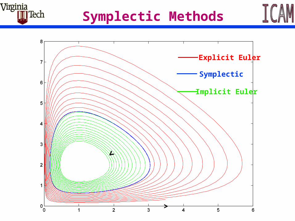
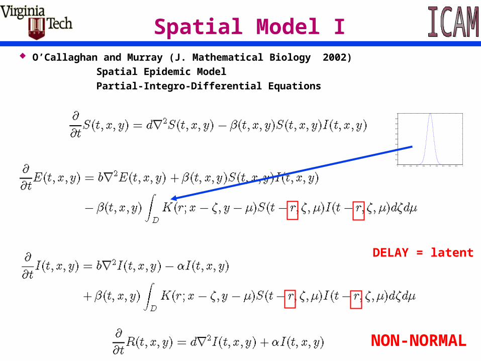
Computational Methods for Design Lecture 2 – Some “Simple” Applications

John A. Burns

Center for Optimal Design And Control

Interdisciplinary Center for Applied MathematicsVirginia Polytechnic Institute and State University

Blacksburg, Virginia 24061-0531

A Short Course in Applied Mathematics

2 February 2004 – 7 February 2004

N∞M∞T Series Two Course

Canisius College, Buffalo, NY

Today’s Topics

Lecture 2 – Some “Simple” Applications A Falling Object: Does F=ma ? Population Dynamics System Biology A Smallpox Inoculation Problem Predator - Prey Models A Return to Epidemic Models

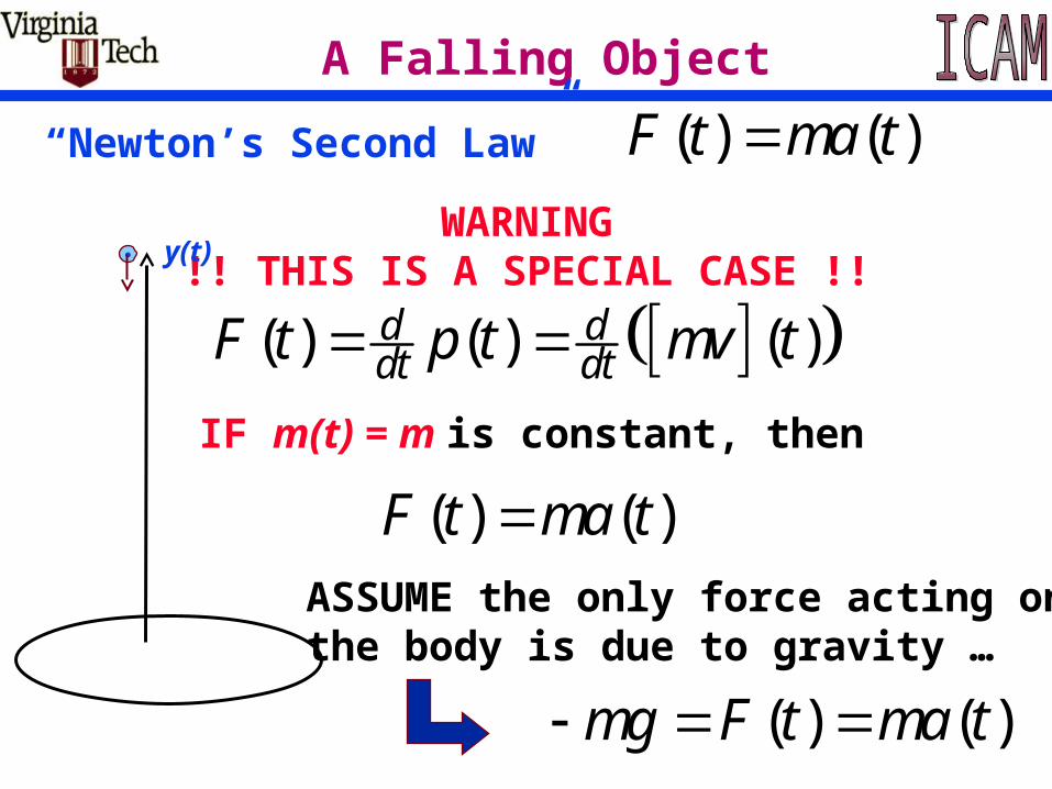
A Falling Object

( ) ( )F t ma t“Newton’s Second Law”

WARNING!! THIS IS A SPECIAL CASE !!

( ) ( ) ( )d ddt dtF t p t mv t

IF m(t) = m is constant, then

( ) ( )F t ma t

( ) ( )mg F t ma t

ASSUME the only force acting onthe body is due to gravity …

. y(t)

A Falling Object (constant mass)

( ) ( ) ( ) ( )d ddt dtmg m t v t m y t my t

. y(t)

( )y t gODE

0 0(0) (0)y h y v INITIAL VALUES

2( ) / 2y t gt at b GENERAL SOLUTION

20 0( ) / 2y t gt v t h

A Falling Object: Problems?

0 5 10 15 20 250

1000

2000

3000

4000

5000

6000

7000

8000

9000

10000

(0) 10,000 (0) 0y y

( )y t

A Falling Object: Problems?

0 5 10 15 20 25-900

-800

-700

-600

-500

-400

-300

-200

-100

0

( ) ( )v t y t

(0) 10,000 (0) 0y y

800 ft/sec 445 m/hr

Terminal Velocity

( ) ( ) ( ) ( ) ( )g dampmy t F t F t mg y t y t AIR RESISTANCE( ) ( )v t y t

( ) 0v t FOR A FALLING OBJECT

( ) ( ) ( )mv t mg v t v t

2( ) ( )mv t mg v t

2 /

2 /

1( )

1

t g mmg

t g m

ev t

e

Terminal Velocity2 /

2 /

1( )

1

t g mmg mgt

t g m

ev t

e

220 ft/sec 150 m/hr

( ) ( )v t y t

Comments About Modeling

( ) ( )ddt mv t F t

Newton’s Second Law IS Fundamental

TWO PROBLEMS1. FINDING ALL THE FORCES (OF IMPORTANCE)2. KNOWING HOW MASS DEPENDS ON VELOCITY

ASSUMING CONSTANT MASS

( )mv t mg( ) ( ) ( )mv t mg v t v t “CORRECTION” FOR AIR RESISTANCE

THE “MODEL” FOR AIR RESISTANCEIS AN APPROXIMATION TO REALITY

More Fundamental Physics

? HOW DOES THE MASS DEPENDS ON VELOCITY ?

186,000 mi/secc

FOLLOWS FORM EINSTEIN’S FAMOUS ASSUMPTION

2E mc

( ) ( ) ( )dE t F t v t

dt

2 ( ) ( ) ( )d d

mc t mv t v tdt dt

2 ( ) ( ) ( ) ( )d d

c m t m t mv t mv tdt dt

More Fundamental Physics

EINSTEIN’S CORRECTED FORMULA

22 2 2 2( ) ( ) ( ) ( )c m t mv t C m t v t C 2 2

0 0c m C C

22 2 2 20( ) ( )c m t mv t c m

22 2

02

( )( ) 1

v tm t m

c

0

2 2( )

1 ( ) /

mm t

v t c

Comments About Mathematics

0

2 2( )

1 ( ) /

mm t

v t c

ONLY IMPORTANT WHEN STILL DOESN’T HELP WITH MODELING FORCES SCIENTISTS AND ENGINEERS MUST FIND THE

“IMPORTANT” RELATIONSHIPS

v c

( ) ( ) ( )dampF t y t y t

MATHEMATICIANS MUST DEVELOP NEW MATHEMATICS TO DEAL WITH THE MORE

COMPLEX PROBLEMS AND MODELS

Comments About Modeling

MORE ACCURATE – MORE COMPLEX – MORE DIFFICULT

)()()( tytym

gty (0) 10,000 (0) 0y y

)(ty)()( tytv

4465

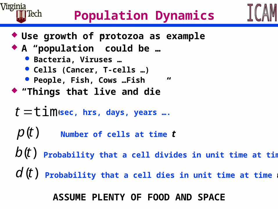
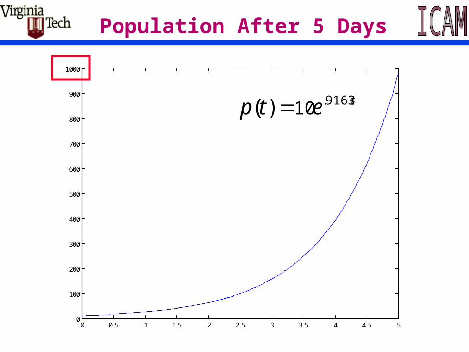
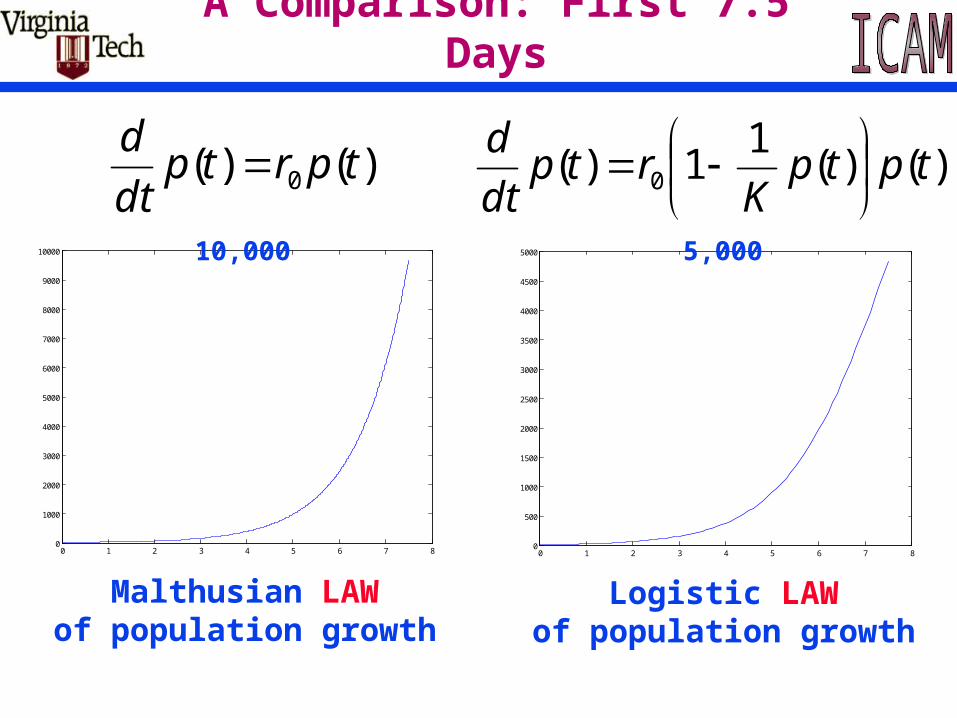
Population Dynamics Use growth of protozoa as example A “population” could be …

Bacteria, Viruses … Cells (Cancer, T-cells …) People, Fish, Cows …Fish

“Things that live and die”

ASSUME PLENTY OF FOOD AND SPACE

)(

)(

)(

time

td

tb

tp

t sec, hrs, days, years ….

Number of cells at time t

Probability that a cell divides in unit time at time t

Probability that a cell dies in unit time at time t

Population Dynamics

ttptb )()(Number of new cells on ttt ,

ttptd )()(Number of cell deaths on ttt ,

ttptbttptbtpttp )()()()()()(Change in cell population

)()()()()()()(

tptrtptdtbt

tpttp

TAKE LIMIT AS 0t

Malthusian LAWof population growth

)()()( tptrtpdt

d

Thomas R. Malthus (1766-1834)

Population Dynamics

000

0

0

)(

)(

)(

dbrtr

dtd

btb

)()( 0 tprtpdt

d

)(

)(

)(

tr

td

tb BIRTH RATE

DEATH RATE

REPRODUCTIVE RATE

00)( petp tr

ASSUMECONSTANT

DO AN EXPERIMENT

10)0( 0 pp

2510)1( 10 rep

5.210

250 re

)5.2ln(ln 00 rer

9163.00 r

Population After 5 Days

0 0.5 1 1.5 2 2.5 3 3.5 4 4.5 50

100

200

300

400

500

600

700

800

900

1000

tetp 9163.10)(

Population After 7.5 Days

0 1 2 3 4 5 6 7 80

1000

2000

3000

4000

5000

6000

7000

8000

9000

10000

tetp 9163.10)(

Population After 10 days

0 1 2 3 4 5 6 7 8 9 100

1

2

3

4

5

6

7

8

9

10x 10

4

tetp 9163.10)(

NOT WHAT REALLY

HAPPENS

Improved Model

COMPETITION FOR FOOD AND SPACE

MalthusASSUMED

PLENTY OF FOOD AND SPACE

Pierre-Fancois Verhulst (1804-1849)

)()( ,)( 1010 tpddtdp(t)bbtb

)(1

1)(1)( 00

110 tp

Krtp

r

dbrtr

)()()()( 1100 tpdbdbtdtbtr

Logistics Equation

)()()( tptrtpdt

d

11

0

db

rK

)(

11)( 0 tp

Krtr

11

0

db

rK

CARRYING CAPACITY

NATURAL REPRODUCTIVE RATE

)()(1

1)( 0 tptpK

rtpdt

d

LE

IS THIS A BETTER(MORE ACCURATE)

MODEL? ?

A Comparison: First 5 Days

0 0.5 1 1.5 2 2.5 3 3.5 4 4.5 50

100

200

300

400

500

600

700

800

900

1000

tetp 9163.10)(

Malthusian LAWof population growth

)()( 0 tprtpdt

d )()(

11)( 0 tptp

Krtp

dt

d

0 0.5 1 1.5 2 2.5 3 3.5 4 4.5 50

100

200

300

400

500

600

700

800

900

1000

)(tp

Logistic LAWof population growth

A Comparison: First 7.5 Days

0 1 2 3 4 5 6 7 80

1000

2000

3000

4000

5000

6000

7000

8000

9000

10000

Malthusian LAWof population growth

0 1 2 3 4 5 6 7 80

500

1000

1500

2000

2500

3000

3500

4000

4500

5000

Logistic LAWof population growth

)()( 0 tprtpdt

d )()(

11)( 0 tptp

Krtp

dt

d

10,000 5,000

A Comparison: First 10 Days

0 1 2 3 4 5 6 7 8 9 100

1000

2000

3000

4000

5000

6000

7000

8000

9000

Logistic LAWof population growth

)()( 0 tprtpdt

d )()(

11)( 0 tptp

Krtp

dt

d

Malthusian LAWof population growth

0 1 2 3 4 5 6 7 8 9 100

1

2

3

4

5

6

7

8

9

10x 10

4

9,000100,000

Logistic Equation: 15 Days

0 5 10 150

1000

2000

3000

4000

5000

6000

7000

8000

9000

10000

)(tp

)()(1

1)( 0 tptpK

rtpdt

d

K

Modeling in Biology

Malthusian LAWof population growth

Logistic LAWof population growth

)()( 0 tprtpdt

d )()(

11)( 0 tptp

Krtp

dt

d

MORE ACCURATE – MORE COMPLEX – MORE DIFFICULT

? WHAT HAVE WE LEFT OUT ?? WHAT IS THE CORRECT LAW ?

NEED A NEWTON OR EINSTEINFOR SYSTEM BIOLOGY

))(),(,()( tptptftpdt

d

A Smallpox Inoculation Problem

Basic issue: Compute the gain in life expectancy if smallpox eliminated as a cause if death?

Very timely problem What if smallpox is “injected” into a large city? How does age impact the problem? a = AGE

)(

)(

)(1)(

)(

)(

)(

ay

ax

asac

a

as

a

Fraction of susceptibles who survive & become immune

Death rate at age a due to all causes

Rate at which susceptibles become infected

Fraction that dies due to the infection

Probability that a newborn is alive and susceptible at age a

Probability that a newborn is alive and immune at age a

A Smallpox Inoculation Model

0)0( ),()()()()(1)(

1)0( ),()()()(

yayaaxaacayda

d

xaxaaaxda

d

Typical epidemiological model Contains age dependent coefficients Model applied to Paris

Not funded by Dept. of Homeland Defense Work was done in 1760 and published in 1766 by …

Daniel Bernoulli, “Essai d’une nouvelle analyse de la mortalité causée par la petite vérole”, Mém. Math. Phys. Acad. Roy. Sci., Paris, (1766),1.

Predator - Prey Models

)()()(

)()()(

tdyctytydt

d

tbyatxtxdt

d

Vito Volterra Model (1925) Alfred Lotka Model (1926)

THINK OF SHARKS AND SHARK FOOD

dcba

ty

tx

,,,

)(

)(

Numbers of predators

Numbers of prey

Parameters

2)(tx

Numerical Issues: LV Model

)()()(

)()()(

tdyctytydt

d

tbyatxtxdt

d

Numerical Schemes? Explicit Euler? Implicit Euler? ODE23? ODE45? ??????

a/b

c/d

o

>

>

>

y

xo

Symplectic Methods

Explicit Euler

Symplectic

Implicit Euler

>

>

Epidemic Models

Susceptible Infected

Removed

Epidemic Models SIR Models (Kermak – McKendrick, 1927)

Susceptible – Infected – Recovered/Removed

( ) ( ) ( )dS t S t I t

dt

( ) ( ) ( ) ( )dI t S t I t I t

dt

( ) ( )dR t I t

dt

( ) ( ) ( ) constantS t I t R t N

SIR Models

)()()()()()(

)()()(

tStItItItStIdt

d

tItStSdt

d

constant)()()(

)()(

NtRtItS

tItRdt

d

0)()()(

then,)( If

tStItIdt

d

tS

NOT ISOLATED

NSI ee 0 ,0

Equilibrium

SIR Model

I(t)

S(t)

S(t) + I(t) = N = 1

Epidemic Models (SARS) SEIJR: Susceptibles – Exposed - Infected - Removed

)()()(

)()()(

222

111

tPtSrtSdt

d

tPtSrtSdt

d

)()()(

)()()()(

)()()()(

21

2

1

tJtItRdt

d

tJtItJdt

d

tItkEtIdt

d

)()()()()()( 2211 tkEtPtSrtPtSrtEdt

d

)(/))()()(()( tNtlJtqEtItP

Model of SARS Outbreak in Canada

byChowell, Fenimore, Castillo-Garsow & Castillo-Chavez (J. Theo. Bio.) Multiple cities (patch models)

Hyman Mass transportation

Castillo-Chavez, Song, Zhang Delays

Banks, Cushing, May, Levin … Migration – Spatial effects

Aronson, Diekmann, Hadeler, Kendall, Murray, Wu …

Spatial Model I O’Callaghan and Murray (J. Mathematical Biology 2002)

Spatial Epidemic Model Partial-Integro-Differential Equations

NON-NORMAL

DELAY = latent

-1 -0.8 -0.6 -0.4 -0.2 0 0.2 0.4 0.6 0.8 10

0.1

0.2

0.3

0.4

0.5

0.6

0.7

0.8

0.9

1

Spatial Model II

WHERE A generates a delay semi-groupHERE

Remarks

GOOD COMPUTATIONAL MATHEMATICS WILL BE THE KEY TO FUTURE BREAKTHROUGHSAPPROXIMATIONS MUST BE DONE RIGHT

LOTS OF SIMPLE APPLICATIONS OPPORTUNITIES FOR MATHEMATICIANS TO

GET INVOLVED WITH MODELING = JOB SECURITY FOR APPLIED MATHEMATICIANS NEW MODELS NEED TO BE DEVELOPED …

TOGETHER … MATHEMATICIANS WITH PHYSICS, CHEMISTRY, BIOLOGY … FLUID DYNAMICS, STRUCTURAL DYNAMICS …