San Jose State UniversitySJSU ScholarWorks

Master's Projects Master's Theses and Graduate Research

Fall 2012

Computational Modeling of Protein Dynamicswith GROMACS and JavaMiaoer YuSan Jose State University

Follow this and additional works at: http://scholarworks.sjsu.edu/etd_projects

Part of the Computer Sciences Commons

This Master's Project is brought to you for free and open access by the Master's Theses and Graduate Research at SJSU ScholarWorks. It has beenaccepted for inclusion in Master's Projects by an authorized administrator of SJSU ScholarWorks. For more information, please contactscholarworks@sjsu.edu.

Recommended CitationYu, Miaoer, "Computational Modeling of Protein Dynamics with GROMACS and Java" (2012). Master's Projects. 267.http://scholarworks.sjsu.edu/etd_projects/267

Computational Modeling of Protein Dynamics with

GROMACS and Java

A Project

Presented to

The Faculty of the Department of Computer Science

San Jose State University

In Partial Fulfillment

of the Requirements for the Degree

Master of Computer Science

By

Miaoer Yu

December 2012

2

©2012

Miaoer Yu

ALL RIGHTS RESERVED

3

APPROVED FOR THE DEPARTMENT OF COMPUTER SCIENCE

Dr. Sami Khuri, Department of Computer Science, SJSU Date

Dr. Chris Pollett, Department of Computer Science, SJSU Date

Natalia Khuri, Bioengineering and Therapeutic Sciences, UCSF Date

4

ABSTRACT

Computational Modeling of Protein Dynamics with GROMACS and Java By Miaoer Yu

GROMACS is a widely used package in molecular dynamics simulations of biological molecules such as proteins, and nucleic acids, etc. However, it requires many steps to run such simulations from the terminal window. This could be a challenge for those with minimum amount of computer skills. Although GROMACS provides some tools to perform the standard analysis such as density calculation, atomic fluctuation calculation, it does not have tools to give us information on the specific areas such as rigidity that could predict the property of the molecules. In this project, I have developed a user friendly program to carry out molecular dynamics simulations for proteins using GROMACS with an easy user input method. My program also allows one to analyze the rigidity of the proteins to get its property.

5

ACKNOWLEDGMENTS

I would like to thank my project advisor Dr. Sami Khuri for countless suggestions and

encouragement. I would also like to thank Dr. Chris Pollett for his suggestions and

comments on my project. I am especially thankful to Natalia Khuri at UCSF, whose

advice and ideas were essential to the completion of my project.

6

Table of Contents

1. Introduction to Molecular Dynamics Simulation 7

2. GROMACS Overview 13

3. Java Application Design and Implementation 21

4. Applications 32

5. Conclusions 50

6. Future work 51

7. References 52

7

1. Introduction to Molecular Dynamics Simulation

Molecular dynamic simulation is a computational method that simulates the motion

of a system of particles. McCammon introduced the first protein simulations in 1977, and

since then this method has been widely used in the theoretical study of biological

molecules including proteins and nucleic acids because it can provide molecular change

information by calculating the time dependent behavior of a molecular system [1, 2]. For

example, GROMACS is a package that carries out molecular dynamic simulations, and

generates a trajectory of the molecule. GROMACS’s high performance draws a lot of

interest from researchers looking to develop their own tools to analyze the GROMACS

trajectories. JGromacs, one of many applications written in the different languages from

that used by GROMACS, analyzes the trajectories generated by GROMACS. JGromacs

does not work with large molecules due to its huge memory consumption. In our project,

we attempt to simplify the GROMACS steps, and develop our own analysis tool that

works well with large molecules.

The goal of a molecular dynamics simulation is to predict macroscopic properties

such as pressure, energy, heat capacities, etc. from the microscopic properties including

atomic positions and velocities generated by molecular dynamic simulations. The bridge

between macroscopic properties and microscopic properties is statistical mechanics using

the time independent statistical average [1]. A molecular dynamics simulation generates a

sequence of points in a multidimensional space as a function of time, where the points

belong to the same collection of all possible systems which have different mechanical

states such as positions or coordinates, and have the same thermodynamic state such as

temperature, volume, pressure [1].

In statistical mechanics, an ensemble averages corresponding to experimental

observables, and this means the molecular dynamics simulations must calculate all

possible states of the system to get the ensemble averages [1]. “The Ergodic hypothesis,

which states that the time average equals the ensemble average,” allows the molecular

dynamics simulation with enough representative conformations to calculate information

on macroscopic properties using a feasible amount of computer resources [1].

8

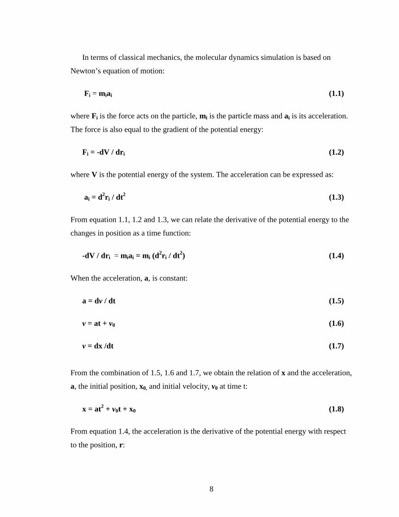
In terms of classical mechanics, the molecular dynamics simulation is based on

Newton’s equation of motion:

Fi = miai (1.1)

where Fi is the force acts on the particle, mi is the particle mass and ai is its acceleration.

The force is also equal to the gradient of the potential energy:

Fi = -dV / dri (1.2)

where V is the potential energy of the system. The acceleration can be expressed as:

ai = d2r i / dt2 (1.3)

From equation 1.1, 1.2 and 1.3, we can relate the derivative of the potential energy to the

changes in position as a time function:

-dV / dr i = miai = mi (d

2r i / dt2) (1.4)

When the acceleration, a, is constant:

a = dv / dt (1.5)

v = at + v0 (1.6)

v = dx /dt (1.7)

From the combination of 1.5, 1.6 and 1.7, we obtain the relation of x and the acceleration,

a, the initial position, x0, and initial velocity, v0 at time t:

x = at2 + v0t + x0 (1.8)

From equation 1.4, the acceleration is the derivative of the potential energy with respect

to the position, r :

9

a = (-dE/dr) / m (1.9)

We can obtain the initial positions of the atoms from experimental structures, such as

the x-ray crystal structure of the molecule, the acceleration from the gradient of the

potential energy function, and the initial distribution of velocities from:

N

P = ∑mivi = 0 (1.10) i=1

where P is momentum, vi is the velocities that are often chosen randomly from a

Maxwell-Boltzmann or Gaussian distribution at a given temperature [1].

The potential energy is a function of the atomic positions of all the atoms in the

system. Because this function is complicated, it must be solved numerically with

numerical algorithms such as Verlet algorithm, Leap-frog algorithm, Velocity Verlet,

Beeman’s algorithm, etc [1].

In [1], those algorithms are introduced. “All of those algorithms assume the positions,

velocities and accelerations can be approximated by a Taylor series expansion:

r(t + δδδδt) = r(t) + v(t)δδδδt + (1/2)a(t) δ δ δ δt2 + … (1.11)

v(t + δδδδt) = v(t) + a(t)δδδδt + (1/2)b(t) δ δ δ δt2 + … (1.12)

a(t + δδδδt) = a(t) + b(t)δδδδt + … (1.13)

where r is the position, v is the velocity, a is the acceleration, etc.”

For example, to derive the Verlet algorithm, we can write:

r(t + δδδδt) = r(t) + v(t)δδδδt + (1/2)a(t)δδδδt2 (1.14)

r(t - δδδδt) = r(t) - v(t)δδδδt + (1/2)a(t)δδδδt2 (1.15)

Combining 1.14 and 1.15, we obtain:

10

r(t + δδδδt) = 2r(t) – r(t – δδδδt) + a(t)δδδδt2 (1.16)

This algorithm uses positions and acceleration at time t and the positions from time t

– δt to calculate the new positions at time t + δt.

The available potential energy functions such as the AMBER, CHARMM,

GROMOS, OPLS / AMBER, etc. provide reasonably good accuracy with reasonably

good computational efficiency [1]. Therefore, we have the needed information to

calculate the trajectory that describes the positions, velocities and acceleration of the

particles at different time, and we can determine the detailed information about the

molecules [1].

In general, there are three stages in molecular dynamics simulation: preparation of the

input, production molecular dynamics, and analysis of the result (Figure 1) [3].

Stage I: Preparation

This stage has multiple steps including generating the topology file; defining a box

and filling it with solvent, and adding any counter-ions to neutralize the system;

performing energy minimization to provide stable simulation; performing equilibration

for sufficient time to get stable pressure, temperature and energy [3].

Stage II: Production

This stage is the longest stage resulting in a trajectory containing coordinates and

velocities of the system.

Stage III: Analysis

The last stage includes analysis of the resulting trajectory and data files to obtain

information on the property of the molecule. Some important quantities calculated in this

stage include RMS difference between two structures, RMS fluctuations, and rigidity or

constant force, etc. The equations used to calculate those quantities are listed as the

following [1, 4]:

11

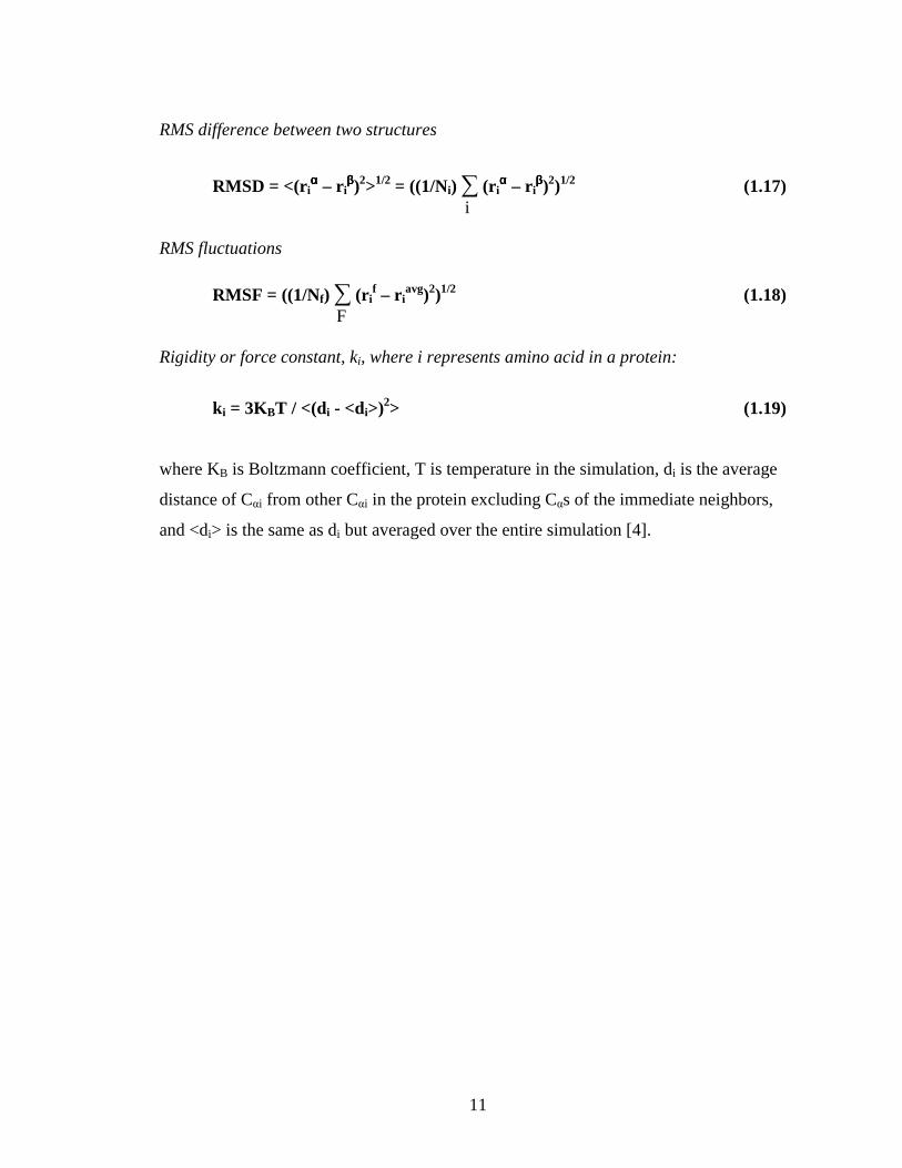
RMS difference between two structures

RMSD = <(riαααα – ri

ββββ)2>1/2 = ((1/Ni) ∑ (r iαααα – ri

ββββ)2)1/2 (1.17) i RMS fluctuations

RMSF = ((1/Nf) ∑ (r if – ri

avg)2)1/2 (1.18) F Rigidity or force constant, ki, where i represents amino acid in a protein:

k i = 3KBT / <(di - <di>)2> (1.19)

where KB is Boltzmann coefficient, T is temperature in the simulation, di is the average

distance of Cαi from other Cαi in the protein excluding Cαs of the immediate neighbors,

and <di> is the same as di but averaged over the entire simulation [4].

12

Among many molecular dynamics simulation packages, GROMACS, CHARMM,

AMBER, and NAMD are most commonly used [5]. We will use GROMACS in our study

because it is open-source, and popular in the study of protein. Before we develop a tool to

analyze the GROMACS data, we need to understand GROMACS. In the next section, we

will introduce GROMACS and its features.

Analysis

Production MD

Equilibration

Generate Topology

Define Box and Solvate

Add Ions

Energy Minimization

Stage I

Stage II

Stage III

Figure 1. Three stages in molecular dynamic simulation: preparation of the input, production molecular dynamic and analysis of the result.

13

2. GROMOCS Overview

GROMACS is an acronym for GROningen Machine for Chemical Simulation. It was

developed at the University of Groningen, The Netherlands, in the early 1990s [6]. This

open-source project is written in ANSI C, and contains about 100 utility and analysis

programs which allow users to perform molecular simulations and energy minimization

(EM) for biological molecules [6]. It is one of the most commonly used molecular

dynamics simulation packages. The following is a list of the main features the

GROMACS has [7, 8].

1. Features for generating topologies and coordinates [7, 8]

pdb2gmx – converts pdb files to topology and coordinate files.

editconf – edits the box and writes subgroups

genbox – solvates a system

genion – generates mono atomic ions on energetically favorable positions

2. Features for running a simulation [7, 8]

grompp – makes a run input file

mdrun – performs a simulation, does a normal mode analysis or an EM.

3. Features for processing properties [7, 8]

g_energy – writes energies to xvg files and displays averages

g_gyrate – calculates the radius of gyration

g_potential – calculates the electrostatic potential across the box

g_density – calculates the density of the system

4. Features for processing files [7, 8]

trjconv – converts and manipulates trajectory files

5. Analysis tools [7, 8]

g_rms – calculates rmsd’s with a reference structure and rmsd matrices

14

g_rmsf – calculates atomic fluctuations

The typical GROMACS MD run of the protein such as lysozyme is demonstrated in

the flow chart (Figure 2) [7, 8]. In the flow chart, the steps are listed in the left column,

while the highlighted GROMACS tools are listed in the right column corresponded to the

left column.

To learn how to use GROMACS in MD of the protein, we followed the tutorial for

lysozyme [9]. In this example, PDB file 1AKI.pdb can be downloaded from RCSB

website for hen egg white lysozyme (PDB code 1AKI). The pdb2gmx generates a

topology for the molecule, the position restraint file, and a post-processed structure file.

The lysozyme is simulated in a simple aqueous system. The editconf tool defines the

box dimensions, and the genbox tool fills the box with water. The purpose of the genbox

is to keep track of the number of added water molecules, and update the topology with

the changes [7, 8]. Now the system is solvated and contains a charged protein.

15

16

The tool grompp (GROMACS pre-processor) processes the ions.mdp (molecular

dynamics parameter file), the coordinate file and topology to generate an atomic-level

input (ions.tpr) containing all the parameters for all of the atoms in the system. The

genion tool reads through the topology and replaces water molecules with the ions

specified by the user to neutralize the net charges on the protein [9].

The energy minimization relaxes the structure to ensure that the system has no steric

clashes or inappropriate geometry [9]. The tool grompp assembles the minim.mdp, the

structure, topology to generate an input file (em.tpr), and then the tool mdrun runs the

energy minimization to generate an energy-minimized structure file em.gro, energy file

em.edr and trajectory em.trr. The analysis of em.edr file with the tool g_energy results in

the following graph showing the steady convergence of Epotential (Figure 3) [9].

Figure 3. Energy Minimization for Lysozyme (1AKI).

17

Once we get the reasonable starting structure, we need to equilibrate the solvent and

ions around the protein under an NVT ensemble (the constant Number of particles,

Volume, and Temperature) and an NPT ensemble (the constant Number of particles,

Pressure, and Temperature) [9]. The same tools used in EM step perform the two-phase

equilibration. The tool g_energy processes the result to generate plots for NVT (Figure 4)

and NPT (Figure 5) [9].

Figure 4. Temperature for Lysozyme (1AKI).

Figure 4 shows that the system reaches the target temperature, and stays there over

the remainder of the equilibration. Figure 5 has the fluctuated pressure value. However,

the running average of these data is stable [9].

18

After finishing the preparation stage, the previous tools grompp and mdrun are used

to perform the production MD to generate the final trajectory file md.trr and md.xtc etc.

Figure 5. Pressure for Lysozyme (1AKI).

After finishing the simulation, we can analyze the system with GROMACS tools

trjconv, g_rms, g_rmsf, etc. The RMSD plot obtained with the tool g_rms (Figure 6)

shows that the structure is very stable with stable RMSD. The RMSF plot obtained with

the tool g_rmsf (Figure 7) shows how each residue fluctuates during the period of the

production run [9].

19

Figure 6. RMSD for Lysozyme (1AKI)

Figure 7. RMS Fluctuation for Lysozyme (1AKI).

20

As shown in Figure 2, there are many steps involved in the whole process of

molecular dynamics simulation. Some users may find it difficult to use the GROMACS

from a terminal window. On the other hand, GROMACS provides some tools to perform

the basic analysis of the trajectories, but we could not find tools to give us the

information on the specific areas such as rigidity we are interested in due to its relation to

the protein property [4]. In the next section, we will show the development of a Java

program that simplifies the GROMACS steps through GUIs and processes the trajectories

to give rigidity information of the protein.

21

3. Java Program Design and Implementation

The two goals in this project are to simplify the MD running steps in GROMACS

with GUIs, and to create an analysis tool that processes the GROMACS trajectories and

gives us the rigidity profile of the proteins.

GROMACS is written in the C language, but we will develop our program in Java.

Therefore, we investigated two methods that allow Java to use the codes and code

libraries written in other languages such as C. One involves the Java Native Interface

(JNI), and another involves Java Runtime class. The former requires six steps to call C

from Java code [10]:

1. Create the Java code. The code needs to have declaration of the native method,

load the shared library containing the native code, and then call the native

method.

2. Compile the Java code

3. Create the C header file by running javah –jnj command on the java code

4. Create the C code

5. Compile the C code and create shared library

6. Execute Java program.

The latter involves creating an object of Runtime, and this Runtime object calls the

Runtime method exec(command) where the command can be used to call C functions.

Some codes related to the script call in Runtime are as follows:

Runtime rt = Runtime.getRuntime(); //create an object rt of Runtime

String[] cmds = {scriptName, parm1, parm2}; //command to execute the script

Process process = rt.exec(cmds); //create a process object

process.waitFor(); //wait for the script completion

Since the former is more complicated to implement, we use the latter in our program.

We built the GUIs with the Model-View-Controller (MVC) pattern first described by

Krasner and Pope for building user interfaces in Smalltalk-80 [11]. In MVC, the model

contains data and some tasks, the view presents the data to the user, and the controller

updates the model as necessary when the user interacts with the view [12]. The separation

22

of the three components makes it easy to reuse and maintain the codes. In our program,

we combine the view and the controller in the same class, but separate the data from the

presentation. Due to its large library, containing lots of reusable codes, we wrote the

program in Java, and have our Model to extend the java class Observable that provides

the register/notify infrastructure needed to support the views implementing the java

interface Observer [12]. When the view sees a user interaction, the listeners registered by

the controller are called, and then the controller calls the mutator methods of the model to

update its state, and the model calls setChanged() and notifyObservers() after it has

changed the state. NotifyObservers() will notify the registered observer that the change

has been made, and the observer containing the required update method will make the

change to itself [12].

The class diagram of the project is illustrated in Figure 8. Our program consists of

three subpackages including task, data and gui. The task package contains the classes for

distance calculation, rigidity calculation and the regular file processing; the data package

contains the classes that represent the binary structural data such as the trajectory file,

structure file, etc. and the gui package contains the different view/controller classes that

allow users to enter their settings for the simulations, and the model class that stores the

user inputs.

The program communicates with the users for their inputs starting with

MainPanelView class. The MainPanel view is illustrated in Figure 9.

23

Figure 8. UML class diagram of the project.

24

Figure 9. Initial panel view.

Six function buttons including “Home”, “Preparation”, “Production Run”, “Auto

Run”, “Plot”, and “Exit” are listed on the left column of the page, and the help function

button is in the upper left corner. The user can select the specific function by clicking on

the button labeled with the name of the function. After the user selects the function, the

corresponding page will be displayed for the user inputs.

When the user clicks on Home, Figure 9 is displayed. The user enters the MD folder,

and the program later will store the files created during the MD preparation and

production.

When the user clicks on Preparation, the Preparation page will be displayed for the

required and optional files and parameters (Figure 10). The user can either provide the

pdb file or the PDB code of the protein. If the user gives both, the pdb file will be used.

Four mdp files including ions mdp, EM mdp, NVT mdp and NPT mdp are required in

this stage. If the user does not specify the file paths, we will use the default files

contained in the package.

25

Figure 10. PreparationView panel.

When the user clicks on Production run, the MD Production page will be displayed

for the required and optional files and parameters (Figure 11). If the user does not provide

the file paths, we will use the default MD mdp contained in the package, and the NPT gro

file, topology resulting from the preparation stage in the MD folder, and default options

and output tpr file name.

Figure 11. ProductionView panel.

26

When the user clicks on Analysis, the analysis page will display three basic analysis

tools (Figure 12). If the user clicks on RMSD, RMSF, or Rigidity, the corresponding tool

page will be displayed under the analysis page (Figure 13, Figure 14, and Figure 15).

Figure 12. AnalysisView panel.

Figure 13. RMSDView panel.

The RMSD view also displays the default options, and the output xvg file name.

27

Figure 14. RMSFView panel with default output xvg file name.

Figure 15. RigidityView Panel.

The rigidity view allows the users to choose the region of the protein they want to

study, or/and the frames they want to consider since the frames at the beginning of the

simulation are not stable and could be ignored. If the users don’t provide any input, we

28

will use the default mdp file, the NPT gro file, and the trajectory file resulting from the

previous MD run.

Figure 16. PlotView panel.

When the user clicks on the Plot button, the user is asked to input the data file, and

the program displays the requested rigidity profile plot labeling the amino acids with high

rigidity (Figure 16). If the user wants to take the default settings, he/she can click on the

Auto Run button, and then enter the pdb file or pdb code on the corresponding page. The

program will run the steps included in preparation and production stages with the default

settings. The user can exit the program by clicking the exit button.

To simplify the MD process, we prepared scripts that execute the MD steps (see

Attached CD). After the user enters the input or takes the default values, and then clicks

on the submit button, the program will run the scripts in Java Runtime. It is crucial to

realize that although GROMACS is written in the C language, Java Runtime class allows

users to conduct their GROMACS research in a Java environment. In this way, the user

does not need to exit the program to have a MD run in another environment.

The second goal of this project is to process the trajectories to get the rigidity profile

of the protein. As mentioned before, we use Boltzmann coefficient and the distance of the

29

backbone carbon (Cα) of the protein from other backbone carbons (Cαs) in the protein in

the calculation of the rigidity.

We need to obtain the coordinate information from the binary structural data file

containing the trajectories, and then use the information to calculate the rigidity of the

protein. The resulting rigidity profile can be used to describe the mechanical properties of

the protein.

There are many packages, such as Biojava, StatAlign, Jmol and JGromacs, written in

Java for bioinformatics analysis [5]. Among those packages, JGromacs has a much

smaller API because it is designed to focus on the specific functionalities such as

analyzing GROMACS trajectories [5]. We thought we would find the right tool for

reading the GROMACS trajectory file to get the coordinate information of the alpha

carbons. However, it has very low performance when it processes the large trajectory file

of the large protein. We successfully used JGromacs to process the trajectory file of

lysozyme that has 129 amino acids. However, when we ran the simulation with longer

proteins that are more than 600 residues long, the computer took much longer, and the

resulting trajectory file is much larger.

JGromacs parses the trajectory file via the use of GROMACS tool gmxdump with

Java Runtime class. What the gmxdump does is to read a trajectory file and print that to

standard output in a readable format [7]. JGromacs calls the gmxdump function and reads

the information from the standard output, and then stores the information in memory. In

general, MD simulations of proteins generate a huge trajectory file. When we incorporate

JGromacs in our package, the machine is very slow with a small protein or hangs with a

large protein. We cannot use JGROMACS in our program due to its low performance in

input/output (IO) caused by huge memory consumption.

To get the coordinates of the alpha carbons of the protein, we must find an efficient

way to read the trajectory file. The file with trr file extension contains the trajectory of a

simulation. All the coordinates, velocities, forces and energies are printed as specified in

the mdp file. The trr file in GROMACS contains many frames of data, and each frame

has the same data structure as follows [7]:

int magic; // magic number

30

int sLen; // the String version length

int linefeed; // line feed

String version = ""; // version

int ir_size; // Backward compatibility

int e_size; // Backward compatibility

int box_size; // Non zero if a box is present

int vir_size; // Backward compatibility

int pres_size; // Backward compatibility

int top_size; // Backward compatibility

int sym_size; // Backward compatibility

int x_size; // Non zero if coordinates are present

int v_size; // Non zero if velocities are present

int f_size; // Non zero if forces are present

int natoms; // The total number of atoms

int step; // Current step number

int nre; // Backward compatibility

float t; // Current time

float lambda; // Current value of lambda

float [][] box;

float [][] vir;

float [][] pres;

float [][] coordinates;

float [][] velocities;

float [][] forces;

From the MD mdp file, we can calculate the total number of frames stored in the

trajectory file with formula:

Total number of frames = nsteps / nstxout + 1

where nsteps and nstxout are the parameters found in the MD mdp file. With Java API,

we can easily get the size of the trr file in bytes, and hence a frame in bytes. Therefore,

we can know the offset of each frame in the file. The offset, the data structure of the

frame, and the alpha carbon index obtained from the NPT gro file allow us to get the

coordinate information of the alpha carbons.

To solve the memory consumption problem found in JGromacs, we load one frame of

information to the buffer at a time, extract the coordinate data of the alpha carbons, and

31

then store the coordinates in an array. In this way, the size of the data we process is very

small. Hence, the performance is increased.

To compare the performance between the JGROMACS and our method in getting the

coordinate information, we wrote a small program to get the information from a

trajectory file with JGROMACS’s strategy since we can not directly use JGROMACS

due to its exception with large protein. The following table demonstrates the performance

of two methods on getting the coordinates of the alpha carbons from a trr file of size 13G

resulting from the 10 ns molecule dynamics simulation of PCSK9 protein (Table 1).

Table 1: Comparison of two methods

JGROMACS Method MYGromacs Method

Time (second) 5008 102

The result indicates our method increases the performance about 50 times.

In summary, we improve the performance by two strategies: to divide the large

amount of structural data into frames of data and process one frame of data at a time; and

to limit the number of objects created for each entry in the trajectory file by storing the

information in an array. The codes are documented in the attached CD.

In the next section, we will demonstrate the rigidity profile of the lysozyme and

compare its property with the RMS fluctuation property obtained from the GROMACS

tool. After we confirm the reliability of our program with the well studied lysozyme, we

will perform the similar study on the PCSK9 compounds that play important roles in

cholesterol metabolism.

32

4. Applications

I. PCSK9 Introduction

Cholesterol is an important component of cellular membranes and is a precursor of

steroid hormones and bile acids. It has been extensively studied due to its strong

correlation with blood and heart diseases. Both dietary cholesterol and that are

synthesized de novo are transported by the circulation in lipoproteins [13]. Familial

hypercholesterolemia (FH) is a genetic hyperlipidermia that is characterized by high

levels of plasma cholesterol carried by low-density lipoprotein (LDL) [14]. LDL is the

main cholesterol transport protein in plasma, and the endocytosis of cholesterol-rich LDL

can be mediated by LDL receptor (LDLr) [14]. FH is most commonly caused by

mutations in the gene encoding the LDLr. It is also caused by mutations in three more

genes encoding Apoprotein B-100, ARH adapter protein, and PCSK9 protease [14].

Figure 17. The four proteins associated with familial hypercholesterolemia. LDLr forms a complex with

Apoprotein B-100 surrounding a cholesterol ester core. In the presence of ARH adapter protein, the

complex enters the cell by the endocytosis of the coated pit. Adapted from Nussbaum et al [14].

As shown in Figure 17, in the process of cholesterol uptake by the LDLr, a

cholesterol ester core is surrounded by apoprotein B-100 to form a protein moiety of

LDL. The mature LDLr binds the moiety, travels to the coated pits, and then enters the

33

cell by endocytosis of the coated pits in the presence of ARH adaptor protein. Once it

enters the cell, LDL is hydrolyzed to release free cholesterol. Therefore, mutations in the

genes encoding LDLr, Apoprotein B-100, PCSK9 and ARH adaptor protein can affect

the cholesterol uptake by the LDLr [11]. The removal of LDL cholesterol from

circulation can be reduced by mutation of LDLr, impairing LDL-LDLr binding caused by

mutations in apoprotein B-100, or impairing the internalization of the LDL-LDLr

complex caused by mutations in the ARH protein, or degradation of the LDLr caused by

the mutations in PCSK9 [14].

According to Nussbaum et al, “the LDLr is a transmembrane glycoprotein mainly

expressed in the liver and adrenal cortex, and plays a key role in cholesterol homeostasis.

Hepatic LDLr clears about 50% of intermediate-density lipoproteins (IDL) and 66% to

80% of LDL from the circulation by endocytosis [14]”. It is worth the effort of studying

the LDLr since elevated plasma LDL levels cause atherosclerosis.

2% ~ 10% LDLr mutations are large insertions, deletion, or rearrangement mediated

by recombination between Alu repeats within LDLr [14]. These mutations decrease the

efficiency of IDL and LDL endocytosis, resulting increasing production of LDL from

IDL, and decreasing hepatic clearance of LDL. Therefore, the clearance of LDL through

LDLr-independent pathways is increased, resulting in atherosclerosis [14]. The effect of

LDL receptor mutations on LDL plasma levels depends on environment, gender, and

genetic background. Diet is the major environment modifier of LDL plasma levels

because dietary cholesterol suppresses the synthesis of LDL receptors and thereby raises

plasma LDL levels [14].

It has been reported that a mutation in PCSK9 is involved in autosomal dominant

hypercholesterolemia (ADH), a rare form of FH without mutations of LDLr and the

ligand binding domain of apoprotein B-100 [15].

PCSK9 has cytogenetic location: 1p32.3 and molecular location on chromosome 1:

base pairs 55,505,148 to 55,530,525 [16]. An enzyme encoded by the PCSK9 gene in

humans has orthologs found across many species. Increased PCSK9 protease activity

causes the degradation of LDL receptor, thereby lowers the level of the receptor in

hepatocytes, and regulates the LDL cholesterol metabolism [15]. Gain-of-function

34

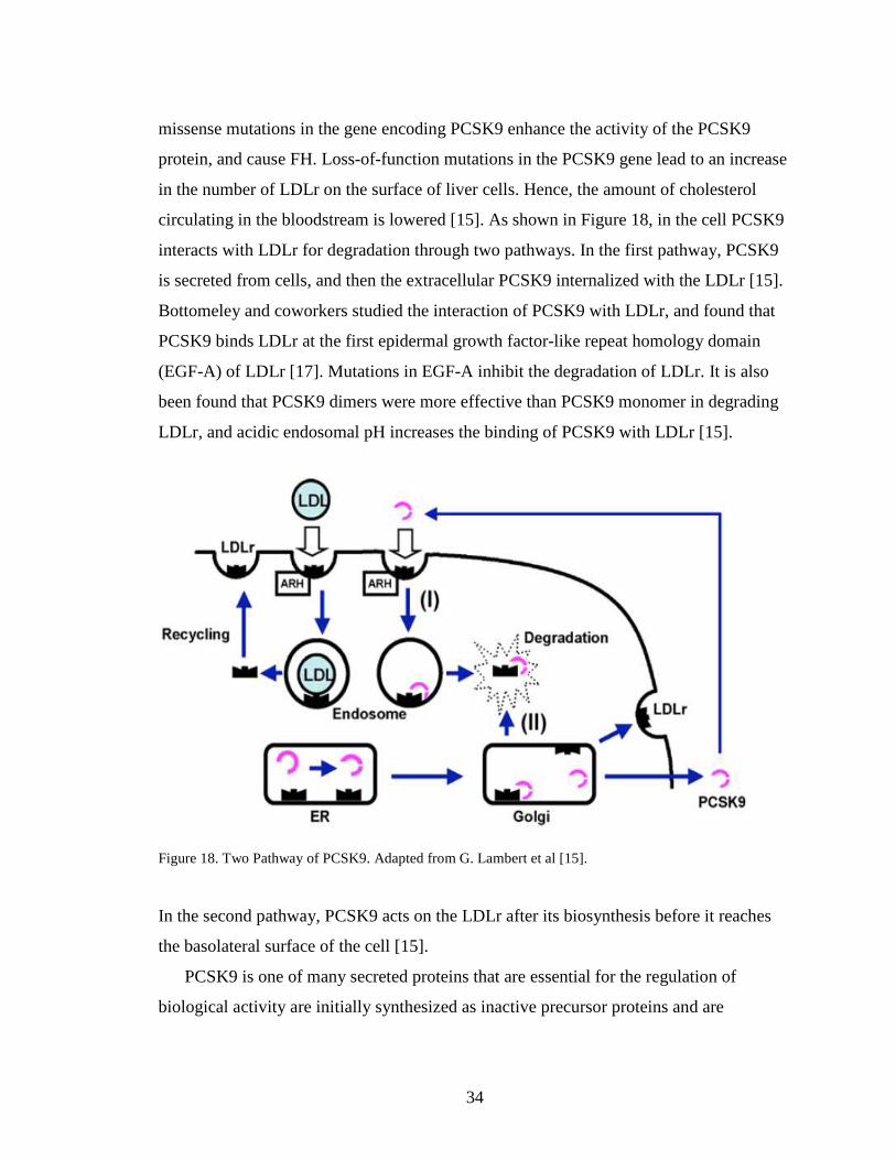
missense mutations in the gene encoding PCSK9 enhance the activity of the PCSK9

protein, and cause FH. Loss-of-function mutations in the PCSK9 gene lead to an increase

in the number of LDLr on the surface of liver cells. Hence, the amount of cholesterol

circulating in the bloodstream is lowered [15]. As shown in Figure 18, in the cell PCSK9

interacts with LDLr for degradation through two pathways. In the first pathway, PCSK9

is secreted from cells, and then the extracellular PCSK9 internalized with the LDLr [15].

Bottomeley and coworkers studied the interaction of PCSK9 with LDLr, and found that

PCSK9 binds LDLr at the first epidermal growth factor-like repeat homology domain

(EGF-A) of LDLr [17]. Mutations in EGF-A inhibit the degradation of LDLr. It is also

been found that PCSK9 dimers were more effective than PCSK9 monomer in degrading

LDLr, and acidic endosomal pH increases the binding of PCSK9 with LDLr [15].

Figure 18. Two Pathway of PCSK9. Adapted from G. Lambert et al [15].

In the second pathway, PCSK9 acts on the LDLr after its biosynthesis before it reaches

the basolateral surface of the cell [15].

PCSK9 is one of many secreted proteins that are essential for the regulation of

biological activity are initially synthesized as inactive precursor proteins and are

35

subsequently proteolytically converted in the secretory pathway to the mature active

forms [18]. These proteinases are called subtilisin-like proprotein convertases (SPCs) or

protein convertases (PCs) because they have subtilisin-like catalytic domain [18]. Protein

convertases are divided into S8A and S8B subfamilies. S8B contains seven closely

related core members including subtilisin/kexin PCSK1, PCSK2, furin, PCSK4, PCSK5,

PCSK6, PCSK7, while S8A contains more distantly related endoproteinases SKI-1/S1P,

PCSK9 [19]. The pro-PCs contain multi domains including a signal peptide, a catalytic

domain, a pro-domain, P-domain, a cysteine-rich domain, transmembrane domain and

cytosolic domain. Each domain has its unique function. The signal peptide directs

translocation into endoplasmic reticulum (ER); the pro-domain has intramolecular

chaperone functions that direct compartment-specific activation, assist in folding of

molecules, disassociate after the second internal cleavage event, and may autoinhibit PCs

in select circumstances; the catalytic domain that contains the conserved catalytic triad

that consists of asparate, histidine and serine; the P-domain may stabilize acidic

prodomain and catalytic domain, and is required for catalytic activity; a cysteine-rich

domain confers protein-protein interaction properties, and directs cell-surface tethering;

the transmembrane domain and cytosolic domain direct PC sorting and transit control

within cell compartments. Transmembrance and cytosolic domains are present only in

furin, PCSK5, PCSK6, PCSK7 [19].

Proprotein convertases activate a broad range of distinct proteins. PCSK1 and PCSK2

activate polypeptide prohormones; Furin activates multiple mammalian and microbial

precursor proteins; PCSK4 activates proteins involved in sperm motility, reproduction;

PCSK5 and PCSK6 activate ECM proteins; PCSK7 activates multiple precursors; SKI-

1/S1P processes membrane-bound transcription factors involved in lipid metabolism; and

PCSK9 regulates plasma LDL levels through increased degradation of LDLr proteins

[19]. Physiologically important proteins may require activation by means of post-

translational cleavage of an inactive precursor molecule. The deficiency of PCSK1 or

PCSK2 results in abnormal glucose homeostasis, and impaired prohormones processing.

PCSK1, PCSK2, furin, PCSK5, PCSK6, PCSK7 have been associated with cancers

through the complex interactions among their activated substrate [19]. PCs also relate to

36

infectious diseases and lipid disorders, atherosclerosis and Alzheimer’s disease, and

biodefense. Therefore, PCs are potential therapeutic targets [19].

According to Lambert et al., “PCSK9 is synthesized as a 72-kDa protein of 692

amino acids in which the signal peptide (residues 1-30) and the prodomain (residue 31 –

152) of PCSK9 precedes a catalytic domain (residues 153 – 451), that contains the

canonical D186, H226 and S386 catalytic triad as well as the oxyanion hole N317

residue, followed by a C-terminal domain (residues 452 – 692) [15]”.

Figure 19. Ribbon structure of PCSK9. Adapted from G. Lambert et al [15].

As shown in Figure 19, the prodomain consists of two α helices and a four-stranded

antiparallel β sheet. The prodomain associates with catalytic domain through

hydrophobic and electrostatic interactions [15]. PCSK9 autocatalytically cleaves the

peptide bond after non-basic amino acids between Gln152 and Ser153 to generate a 14-

kDa prodomain and a 63-kDa moiety [15]. The prodomain are permanently associated

with the 63 kDa PCSK9 moiety, and the four C-terminal amino acids of the prodomain

(residues 149 – 152) bind in the catalytic site and further inhibit the catalytic activity by

N-terminus extension of the prodomain [19]. The catalytic domain consists of seven-

stranded parallel β sheet and α helices. The catalytic triad of PCSK9 consists of residues

Asp186, His226, and Ser386. PCSK9 does not act as a catalyst but as a chaperone that

binds the LDLr at its epidermal growth factor-like repeat A (EGF-A) for lysosomal

37

degradation [15]. The V domain of PCSK9 consists of three barrel-like subdomains that

are made up of antiparallel β strands, and stabilized by three internal disulfide bonds [15].

The V domain is rich in histidine residues that can control the pH-dependent protein-

protein interactions [15].

Researchers have been studying how the mutations in PCSK9 relate to FH. They

reported the disease-associated variants in a database at www.ucl.ac.uk/ [20]. As shown

in Figure 20, the mutations of PCSK9 can be found in any domains of PCSK9.

Figure 20. Number of variants in each domain of the PCSK9 gene according to putative function (n = 73).

Intronic variants have not been included. Adapted from Leigh et al [20].

The selected naturally occurring variants are summarized in Table 2. The loss-of-

function mutations include L82X, Y142X, C679X, DR97, G106R, L253F, N157K and

H391N, while the gain-of-function mutations include D374Y, D374H, S127R, D129G,

F216L, and R218S [15].

The function of PCSK9 is physiologically significant, and it is clinically relevant to

measure circulating levels of PCSK9 and to study pharmacological factors affecting its

secretion. It has been reported that plasma PCSK9 levels correlate positively with LDL

cholesterol but not with HDL cholesterol or TG in healthy donors [15]. PCSK9 has

become a validated target for the treatment of hypercholesterolemia and associated

cardiovascular diseases. Study suggests that pharmacologic interventions that inhibit

38

PCSK9 may be safe. The first approach to inhibit PCSK9 include targeting PCSK9

mRNA that involves the delivery of single-stranded antisense DNA-like chimeric

oligonucleotides via an RNaseH-mediated pathway, and injection of liposomal double

stranded RNA-like siRNAs that interact with the RNA-interference silencing complex

[19, 20, 21].

39

Table 2. PCSK9 naturally occurring variants (X represents stop codon) [20, 22].

The second approach to inhibit PCSK9 directly by molecules includes antibodies or

small interfering RNAs that interfere with PCSK9/LDLr interaction at the plasma

membrane, inhibitors of PCSK9 catalytic activity within the ER, other proprotein

convertases that enhance PCSK9 cleavage, and molecules that destabilize the PCSK9

structure to mimic loss of function mutants [19, 23]. A list of inhibitors of PCSK9

Protein Domain EffectWild Mutant

AA type hydrophobicity AA type hydrophobicity

basic -14 aliphatic 97 p.Leu82X

aliphatic 97 X

basic -14

unique 0 basic -14polar neutral -5 basic -14acidic -55 unique 0

aromatic 63 X

polar neutral -28 basic -23

aromatic 100 aliphatic 97

basic -14 polar neutral -5

aliphatic 97 aromatic 100

acidic -55 aromatic 63

acidic -55 basic 8

polar neutral 49 X

p.Arg46Leu Pro-domain Loss of function, descreased phosphorylation of Ser47

Pro-domain Loss of function, truncated peptide, disrupt proper folding

p.Arg97del Pro-domain Loss of function,disrupts the fold of the entire prodomain.

p.Gly106Arg Pro-domain Loss of function, improper orientation of the beta-strands.

p.Ser127Arg Pro-domain Gain of function, p.Asp129Gly Pro-domain Gain of function p.Tyr142X Pro-domain Loss of function,

truncated peptide, disrupt proper folding

p.Asn157Lys Catalytic Loss of function, could break hydrogen bond and then destabilize the packing of this helix

p.Phe216Leu Catalytic Gain of function can't undergo the second cleavage that can't not induce LDLr degradation.

p.Arg218Ser Catalytic Gain of function can't undergo the second cleavage that can't not induce LDLr degradation.

p.Leu253Phe Catalytic Loss of function, results in a PCSK9 protein that is defective in autoprocessing.

p.Asp374Tyr Catalytic Gain of function, increases in affinity for LDLr by Hydrogen bonding or pi stacking with H306 of EGF-A.

p.Asp374His Catalytic Gain of function, increases in affinity for LDLr by Hydrogen bonding or pi stacking with H306 of EGF-A.

p.Cys679X C-terminal domain

Loss of function, truncated peptide, disrupt proper folding

40

currently undergoing development to reduce the LDL-C levels are summarized in Table 3

[24]. It has been reported that an antibody for PCSK9 (mAb1) administered to wild-type

mice doubled the hepatic content of LDLR and reduced serum total cholesterol by 36%

[24]. Cynomolgus monkeys treated with a single dose of PCSK9 siRNA had a mean

reduction in LDL-C levels of 56% [24].

Table 3: PCSK inhibitors under development [24].

Many other PCs have been studied, especially furin. Comparative study of PCSK9

with well characterized furin and other PCs will be an efficient way to get information

about PCSK9.

II. Comparative study of PCSK9 with other PCs

41

Sun and coworkers reported that the multiple sequence alignment of PCSK9 with

furin and three PCs (PCSK4, PCSK5 and PCSK6) using Clustal2 shows that PCSK9 is

closely resemble to furin [25]. When they compared the key residues in the binding

pocket of furin and those in PCSK9, they found that the obtained multiple sequence

alignment indicated the mutations of PCSK9 including N192 → S, R193 → -, E230 →

Q, V231 → G, E257 → -, A267 → L, S319 → G, S343S → L, P372 → A.

The 3D structure of the furin catalytic domain with an inhibitor complex (Protein

Data Bank ID: IP8J) was created with Chimera 1.6 (Figure 21) [26].

Figure 21. Furin Binding Pocket. Adapted from Sun, et al [25].

The sensitivity and the compensatory effect of the positive charge at substrate

positions P4-P6 requires negatively charged residues in the binding pocket of PCs [25].

Negatively charged residues at position 230 and 257 play a key role in regulation of the

substrate specificity of mammalian proprotein convertases since they interact with a

positively charged residue at substrate position P5 or P6, and facilitate flexible

interactions in this region [25]. It has been reported that cleavage of proprotein

convertases can be inhibited by a small molecule characterized by positively charged

42

residues at substrate position P1, P2, and P4 [25]. This small molecule dec-RVKR-cmk

efficiently binds to all seven 8B proprotein convertases [25]. This methodology can be

used to study the substrate specificity of PCSK9 and find its small molecule inhibitor.

MEGA is used to build a phylogenetic tree for PCSK9 from different species [27].

Figure 22 shows the resulting phylogenetic tree.

43

The information on PCSK9 is valuable, and can be obtained from the PDB website

http://www.rcsb.org/pdb/home/home.do. Table 4 summarizes a list of solved structures of

PCSK9 [28].

Table 4: Solved PCSK9 Structure in PDB

PDB ID Structure Title

2NP9 Crystal structure of a dioxygenase in the Crotonase superfamily

2P4E Crystal Structure of PCSK9

2PMW The Crystal Structure of Proprotein convertase subtilisin kexin type 9 (PCSK9)

2QTW The Crystal Structure of PCSK9 at 1.9 Angstroms Resolution Reveals structural homology

to Resistin within the C-terminal domain

2W2M WT PCSK9-DELTAC BOUND TO WT EGF-A OF LDLR

2W2N WT PCSK9-DELTAC BOUND TO EGF-A H306Y MUTANT OF LDLR

2W2O PCSK9-DELTAC D374Y MUTANT BOUND TO WT EGF-A OF LDLR

2W2P PCSK9-DELTAC D374A MUTANT BOUND TO WT EGF-A OF LDLR

2W2Q PCSK9-DELTAC D374H MUTANT BOUND TO WT EGF-A OF LDLR

2XTJ THE CRYSTAL STRUCTURE OF PCSK9 IN COMPLEX WITH 1D05 FAB

3BPS PCSK9:EGF-A complex

3GCW PCSK9:EGFA(H306Y)

3GCX PCSK9:EGFA (pH 7.4)

3H42 Crystal structure of PCSK9 in complex with Fab from LDLR competitive antibody

3M0C The X-ray Crystal Structure of PCSK9 in Complex with the LDL receptor

3P5B The structure of the LDLR/PCSK9 complex reveals the receptor in an extended

conformation

3P5C The structure of the LDLR/PCSK9 complex reveals the receptor in an extended

conformation

44

Although the number of solved structures is limited, it may take researchers weeks or

months to build the model from the x-ray experimental data. When the molecule becomes

larger and larger, the disadvantage of the experimental method becomes obvious. The

molecular dynamics simulation could be a reasonable method for the study of PCSK9.

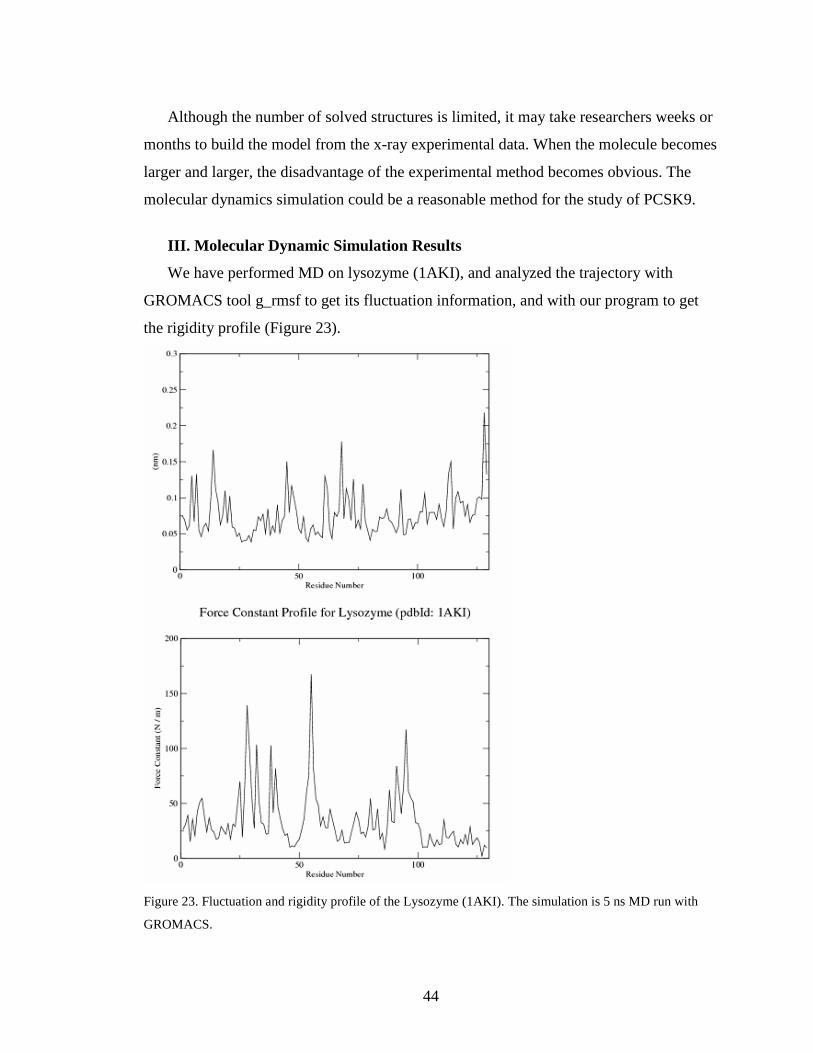
III. Molecular Dynamic Simulation Results

We have performed MD on lysozyme (1AKI), and analyzed the trajectory with

GROMACS tool g_rmsf to get its fluctuation information, and with our program to get

the rigidity profile (Figure 23).

Figure 23. Fluctuation and rigidity profile of the Lysozyme (1AKI). The simulation is 5 ns MD run with

GROMACS.

45

Figure 23 represents the fluctuation and rigidity profile of lysozyme. As seen on the

figure, the residues with high fluctuation often have low rigidity. For example, the strong

rigidity peak is located in the #50 – #55 region where fluctuation is small. This result

confirms our program can correctly predict the rigidity of the residues. We plotted the

rigidity data with our program (Figure 24).We also labeled the predicted high rigidity

residues including Trp28, Ala32, Phe38, Thr40, Ile55, Ser91, and Ala95 in Chimera

image of lysozyme (Figure 25) [29].

Figure 24. Rigidity profile plotted with our program.

46

Figure 25. Residues with high rigidity predicted by our program are Trp28, Ala32, Phe38, Thr40,

Ile55, Ser91, and Ala95. These residues are labeled with 1 letter code and shown in sphere shapes in the

Chimera image of lysozyme (1AKI).

Our program allows the users to easily locate the amino acid residues with high

rigidity by labeling those amino acids above the threshold value set by the user (the

default value is 50% of the maximum value). Both fluctuation and rigidity information

would help us to understand the property of the biological molecule. It has been found

that three amino acid positions beneath the active site are occupied by Thr 40, Ile 55, and

Ser 91 in hen, pheasant, and other avian lysozymes [30] with experimental methods.

These three amino acids can be found among the amino acids with high rigidity predicted

by our program.

The above result on lysozyme indicates our program could be used in the study of

other proteins such PCSK9. We performed the similar study on PCSK9 (PDB code:

2P4E) (Figure 26). Since PCSK9 is a bigger protein with some missing residues in the

initial configuration, we will focus on analyzing the region (#219 – #449) with the

longest unbroken sequence (Figure 27). Within this region, L286, T313, V336, A363,

47

T385, A389 and V392 are predicted to have high rigidity, and there is no reporting

mutation among them [20]. The result indicates the rigidity profile could predict the

conserved region of the protein.

Figure 26. PCSK9 (1AKI) rigidity profile with missing residues located in the disconnected region in the

graph. The simulation is 10 ns MD run with GROMACS.

48

Figure 27. The fluctuation and rigidity profile of PCSK9 partial sequence (#219 - #449).

It has been reported that D374 is the binding location where the PCSK9 forms the

complex with LDLr, and its mutations change its binding efficiency with LDLr [17].

49

Figure 27 indicates D374 has high fluctuation and low rigidity result. We also labeled the

predicted high rigidity residues including L286, T313, V336, A363, T385, A389, and

V392 in Chimera image of PCSK9 (Figure 28) [29].

Figure 28. Residues with high rigidity predicted by our program are L286, T313, V336, A363, T385,

A389, and V392. These residues are labeled with 1 letter code and shown in sphere shapes and located in

the center of the A chain in the Chimera image of PCSK9 (2P4E). The triad residues located on the left of

the center, and D374 are also labeled.

We need more analysis on the pattern of the fluctuation and rigidity on other residues

to find the important information about the binding of the PCSK9 and the LDLr.

50

5. Conclusions

In this project, we learned how to use GROMACS in molecule dynamics simulations.

Through the molecule dynamics simulation of lysozyme using GROMACS, we

understood that the process of running GROMACS in protein dynamics simulations

involves many steps, and GROMACS does not provide a tool to analyze the rigidity of

the protein.

We have developed a Java application to simplify the steps involved in GROMACS.

We investigated two methods that allow us to call C code from Java, and we decided to

use Java Runtime class method since JNI method is too complicated to implement.

Through the graphical user interface (GUI), users can easily carry out molecular

dynamics simulations using GROMACS with their own settings or simply accepting the

default settings given by the program. Our program also allows users to analyze the

GROMACS trajectories to generate the rigidity of the protein, and then plot the rigidity

profile graph with our built-in plotting feature. Compared to JGromacs, our program has

better performance, and works well with the large trajectory files.

We tested our program with lysozyme, and obtained promising results that show the

amino acids involved in the active site of the lysozyme are among the amino acids with

high rigidity. We also used our program in the molecular dynamics simulation of PCSK9,

and found that the amino acids with high rigidity are not among the amino acids that have

reported mutations. These results indicate our program could be used to find the active

site and the conserved amino acids in the protein.

51

6. Future Work

A possible extension of this work would be to continue validating the program with

well studied lysozyme and its variants. This would enable us to find a method to

determine the relationship between the simulation results and the protein property, which

would allow us to expand our study to PCSK9 and its complexes with LDLr to determine

its role in cholesterol metabolism.

Another extension would be to develop a web application of this program that would

allow remote users to access the program.

52

7. References

[1] www.ch.embnet.org/MD_tutorial/ (last retrieved on Feb 1, 2012).

[2] McCammon J.A., Gelin B.R., and Karplus M. Nature 267, 585 (1977).

[3] http://cinjweb.umdnj.edu/~kerrigje/pdf_files/fwspidr_tutor.pdf (last retrieved on

Sep 5, 2012). [4] Stadler AM, Garvey CJ, Bocahut A, Sacquin-Mora S, Digel I, Schneider GJ, Natali

F, Artmann , Zaccai G, J. R. Soc. Interface, 2012 Jun 13.

[5] Munz M., Biggin P.C., J. Chem. Inf. Model. 2012, 52, 255-259.

[6] van der Spoel D., Lindahl E. Hess B., Groenhof G., Mark A.E., and Berendsen

H.J.C., J. Comput. Chem. 26 (16): 1701-18.

[7] Gromacs 4.5 Online Reference, manual.gromacs.org/current/ (last retrieved on Nov

1, 2012).

[8] van der Spoel D., Lindahl E. Hess B., van Buuren A.R., Apol E., Meulenhoff P.J.,

Tieleman D.P., Sijbers A.L.T.M., Feenstra K.A., van Drunen R., and Berendsen

H.J.C., Gromacs User Manual version 4.5.4, www.gromacs.org (last retrieved on

Nov 1, 2012).

[9] http://www.bevanlab.biochem.vt.edu/Pages/Personal/justin/gmx-

tutorials/lysozyme/index.html (last retrieved on Nov 1, 2012)

[10] http://www.ibm.com/developerworks/java/tutorials/j-jni/section2.html (retrieved

on Dec 3, 2012).

[11] Gamma E., Helm R., Johnson R., Vlissides J. Design Patterns: Elements of

Reusable Object-Oriented Software, 1995, Addison-Wesley.

53

[12] http://csis.pace.edu/~bergin/mvc/mvcgui.html. (last retrieved on Nov 1, 2012)

[13] Nelson DL, Cox MM. 2004. Lehninger Principles of Bilchemistry, 4th edition.

Chapter 21.

[14] Nussbaum, McInnes, Willard. 2007. Genetics in Medicine.

[15] Lambert G, Charlton F, Rye K, Piper D, Molecular basis of PCSK9 function,

Atherosclerosis, 2009; 203:1-7.

[16] http://ghr.nlm.nih.gov/gene/PCSK9. (last retrieved on Feb 1, 2012)

[17] Bottomley M, et al. Structural and Biochemical Characterization of the Wild Type

PCSK9-EGF(AB) Complex and Natural Familial Hypercholesterolemia Mutants, j.

Biol. Chem., 284 (2009) 1313-1323.

[18] Henrich S, Lindberg I., Bode W., Than M.E., J. Mol. Biol (2005) 345, 211-227.

[19] Artenstein A, Opal SM, Proprotein Convertases in Health and Disease, The New

England Journal of Medicine, 2011; 365; 26:2507-2518.

[20] Leigh et al. Commentary PCSK9 variants: A new database, Atherosclerosis, 203

(2009) 32-33.

[21] Benjannet et al. The Proprotein Convertase (PC) PCSK9 Is Inactivated by Furin

and/or PC5/6A, Journal of Biological Chemistry, Oct. 2006, vol281(41), page

30561 – 30571.

[22] http://www.sigmaaldrich.com/life-science/metabolomics/learning-center/amino-

acid-reference-chart.html (retrieved on Sep 1, 2012).

[23] Lou KJ, 2009, The secreted secret of PCSK9, SciBX 2(22).

[24] Brautbar, Ballantyne, Pharmacological strategies for lowering LDL cholesterol:

54

statins and beyond. Nature Reviews Cardiology, vol 8, May 2011, page 253 – 265.

[25] Sun et al, Comparative study of the binding pockets of mammalian proprotein

convertases and its implications for the design of specific small molecule inhibitors,

Int. J. Biol. Sci. 2010; 6:89-95.

[26] Pettersen EF, Goddard TD, Huang CC, Couch GS, Greenblatt DM, Meng EC,

Ferrin TE. J Comput Chem. 2004 Oct;25(13):1605-12.

[27] Tamura K., Peterson D., Peterson N., Stercher G., Nei M., Kumar S., Molecular

Biology and Evolution 28: 2731-2739.

[28] www.rcsb.org/pdb/home/home.do (last retrieved on Sep 1, 2012).

[29] UCSF Chimera--a visualization system for exploratory research and analysis.

Pettersen EF, Goddard TD, Huang CC, Couch GS, Greenblatt DM, Meng EC,

Ferrin TE. J Comput Chem. 2004 Oct;25(13):1605-12.

[30] Lescar J., Souchon H., Alzari P.M., Protein Sci. 1994 May; 3(5): 788–798.