ODE-based biomodeling Ion Petre Computational Biomodeling Laboratory Turku Centre for Computer Science Åbo Akademi University Turku, Finland http://combio.abo.fi/ June 20, 2013 1 Bertinoro, Italy
Transcript
ODE-based biomodeling
Ion Petre
Computational Biomodeling Laboratory Turku Centre for Computer Science
Åbo Akademi University Turku, Finland
http://combio.abo.fi/
June 20, 2013 1 Bertinoro, Italy
1. GENERALITIES
June 20, 2013 Bertinoro, Italy 2
The blind men and the elephant
John Godfrey Saxe’s (1816-1887) version of the legend: •First man (feeling the side): like a wall •Second (the tusk): like a spear •Third (the trunk): like a snake •Fourth (the knee): like a tree •Fifth (the ear): like a fan •Sixth (the tail): like a rope
Source: Phra That Phanom chedi, Amphoe That Phanom, Nakhon Phanom Province, northeastern Thailand. Picture downloaded from Wikipedia Author: Pawyi Lee
June 20, 2013 Bertinoro, Italy 3
Modeling
• What is a model? o A (partial) view of the reality o An abstraction of the reality o A representation of the (supposedly) main features of the reality, including the
connections among them
o For a given object of study, many models may be given, possibly focusing on different features of the object
• What a model is not
o A model is not the reality o A model is not certain!
• Many types of models exist!
“All models are wrong, some are useful” Box, G.E.P., Robustness in the strategy of scientific model building, in
Robustness in Statistics, R.L. Launer and G.N. Wilkinson, Editors. 1979, Academic Press: New York.
June 20, 2013 Bertinoro, Italy 4
An example: choose your hypothesis
• From S.Mahajan: Street-fighting mathematics, MIT Press, 2010 • Problem: how many babies (0-2 year olds) are in the US?
o Exact solution: look at the plot with the birth dates of every person in the US
– Huge effort; collected every 10 year by the US Census Bureau
o Approximation – US population: 300 million in 2008 – Assume a life expectancy of 75 (a model where everybody still alive at 75
dies abruptly on their 75th birthday) – Lump the curve into a rectangle: width of 75, height to be calculated
June 20, 2013 Bertinoro, Italy 5
75
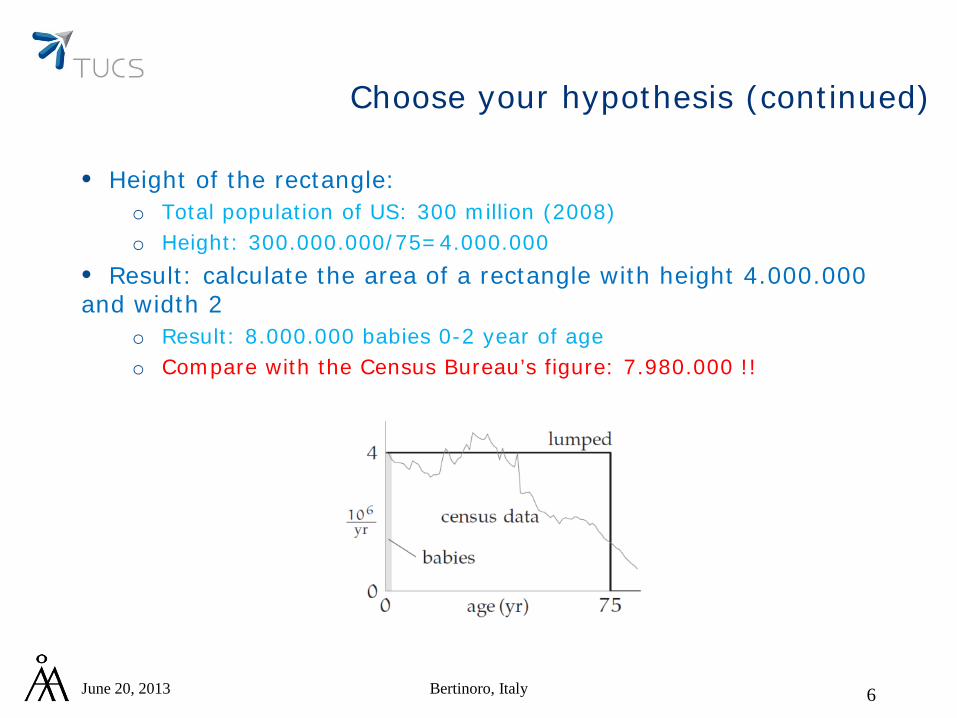
Choose your hypothesis (continued)
• Height of the rectangle: o Total population of US: 300 million (2008) o Height: 300.000.000/75=4.000.000
• Result: calculate the area of a rectangle with height 4.000.000 and width 2
o Result: 8.000.000 babies 0-2 year of age o Compare with the Census Bureau’s figure: 7.980.000 !!
June 20, 2013 6 Bertinoro, Italy
Model: Life inside a cell
Simplifications often made by biomodelers • Cell is “like a bag of chemicals
floating in water” • Metabolites flow around
chaotically • Metabolites are uniformly
distributed • Proteins are just like balls (or
cubes), DNA is just like a rope • In a DNA sequence, A is
always matched with T, C always with G
• Processes are isolated from each other and from the environment
• …
The reality is surprisingly complex • The cell has a skeleton, gives it
flexibility • Many intracellular boundaries,
many specialized organelles • Highly specific metabolites • Very precise recognition of
one’s target • Energy efficiency optimized • Exquisite regulation,
synchronization, signal propagation, cooperation
• Some particles do move chaotically, but some others are transported
• Some aspects are discrete (on/off), some others are continuous-like (always on, variable speed)
• Huge pressure, crowded
A view on “The Inner Life of a Cell” (Harvard University, 2006): Artistic representation of metabolite transportation, protein-protein binding, DNA replication, DNA ligase, microtubule formation/dissipation, protein synthesis, …
June 20, 2013 Bertinoro, Italy 7
Mathematical modeling
• We focus in this lecture on mathematical models o As we saw, (many) other types of models exist o “Model” is indeed a very overloaded word o In this lecture a model is a mathematical representation of the reality o Models that mimic the reality by using the language of mathematics
• Goal of the lecture
o An introduction to the process of mathematical modeling o Give a number of techniques used for:
– Building a model – Analyzing a model
o Main tools: (systems of) ODEs
June 20, 2013 Bertinoro, Italy 8
Mathematical models
• Starting point for modeling: divide the world into 3 parts o Things whose effects are neglected
– Ignore them in the model o Things that affect the model but whose behavior the models is not
designed to study – External variables, considered as parameters, input, or independent
variables o Things the model is designed to study the behavior of
– Internal (or dependent) variables of the model
• Deciding what to model and what not is difficult o Wrong things neglected: the model is no good o Too much included: hopelessly complex model o Choose the internal variables wrongly: the model will not capture its
target o How general should the model be: model a table (any table?) or the
specific table in front of the modeler
June 20, 2013 Bertinoro, Italy 9
Modeling cycle
Real-world data Model
Predictions / explanations
Mathematical conclusions
Analysis Verification
Simplification
Interpretation
June 20, 2013 Bertinoro, Italy 10
Start here
Model validation
• Any model must always be subjected to experimental validation against the reality
• A model may be invalidated by experimental data
• No set of experimental data can confirm the “truthfulness” of a model
June 20, 2013 Bertinoro, Italy 11
2. FORMULATING AN ODE MODEL
June 20, 2013 Bertinoro, Italy 12
Modeling with differential equations
• Modeling strategy o We model the change in the values of all variables: o Future value = present value + change o We describe the change as a function of the current values of all
variables o If the process takes place continuously in time, it leads to differential
equations • Each species s modeled as a function s:R+R+
o Concentrations • Dependencies expressed as systems of ODEs
• Bad news: the equations are often non-linear and in general they cannot be solved analytically
June 20, 2013 Bertinoro, Italy 13
Example: population growth
• Example: population growth (the Malthus model, 18th century)
o Problem: Given a population’s size P0 at time t=t0, predict the population level at some later time t1
o We consider two factors: birthrate and death rate. We ignore immigration and emigration, living space restrictions, food avail, etc.
o Birthrate: influences by many factors, including infant mortality rate, availability of contraceptives, abortion, health care, etc.
o Death rate: influences by sanitation, public health, wars, pollution, medicine, etc.
o Assume that in a small interval of time, a percentage b of the population is newly born and a percentage c of the population dies
o We write an equation for the change in the population: dP/dt = bP(t)–cP(t), i.e., dP/dt=(b-c)P(t)
o The solution is: P(t)=P0exp((b-c)(t-t0))
June 20, 2013 Bertinoro, Italy 14
Example: population growth
• Verifying the model: numerical fit and validation
o Population of US in 1990: 248.710.000 and in 1970: 203.211.926 o Plugging in these numbers, we obtain that b-c=0.01 o Predict the population in 2000: 303.775.080 o The real population level in 2000: 281.400.000. o The model prediction is about 8% off the mark. Not too bad! o Predict the population level in 2300: 55.209.000.000.000!!!
o Conclusion: the model is unreasonable over long periods of time
June 20, 2013 Bertinoro, Italy 15
A refined model for population growth
• In the basic model we have assumed that the change in the population is proportional to the current population level: dP/dt = kP(t)
• Assume that k is not constant
o Assume that it depends on the population level o For example: as the population increases and gets closer to a maximum
level M, k decreases o One possible (simple, linear) model for this: k=r(M-P(t)) o Our equation: dP/dt=r(M-P(t))P(t)
o Such a population model for US was proposed in 1920, with
M=197.273.522, determined based on census figures for 1790, 1850, 1910
o Verifying the model: very good predictions up to 1950, too small predictions for 1970, 1980, 1990, 2000
o Not surprising: immigration, wars, advances in medicine not considered
o Note: Verifying the model on the growth of yeast in culture gives excellent predictions
June 20, 2013 Bertinoro, Italy 16
Giordano et al. A first course in mathematical modeling. (3rd edition), Page 375
June 20, 2013 Bertinoro, Italy 17
Stable and unstable equilibria / steady states
June 20, 2013 Bertinoro, Italy 18
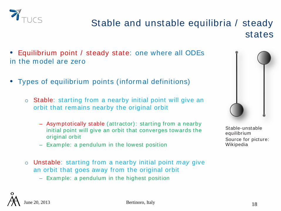
• Equilibrium point / steady state: one where all ODEs in the model are zero
• Types of equilibrium points (informal definitions)
o Stable: starting from a nearby initial point will give an
orbit that remains nearby the original orbit
– Asymptotically stable (attractor): starting from a nearby initial point will give an orbit that converges towards the original orbit
– Example: a pendulum in the lowest position
o Unstable: starting from a nearby initial point may give an orbit that goes away from the original orbit
– Example: a pendulum in the highest position
Stable-unstable equilibrium Source for picture: Wikipedia
Graphical solutions
• Consider autonomous systems of first-order ODEs dxi/dt=fi (x1,x2,…xn) o not time dependent
o consider its solution as describing a trajectory in the n-dimensional plane,
with coordinates (x1(t),x2(t),…,xn(t)) – convenient to think about it as the movement of a particle
o Having an autonomous system implies that the direction of movement
from a given point on the trajectory only depends on that point, not on the time when the particle arrived in that point
– Consequence: only one trajectory going through any given point – Equivalently: two different trajectories cannot intersect – Consequence: no trajectory can cross itself unless it is a closed curve (periodic)
o the n-dimensional plane (x1,x2,…xn) is called a phase plane
June 20, 2013 Bertinoro, Italy 19
Graphical solutions
• Consider autonomous systems of first-order ODEs dxi/dt=fi (x1,x2,…xn)
o if (e1,e2,…en) is an equilibrium point, then the only trajectory going through that point is the constant one
– Consequence: a trajectory that starts outside an equilibrium point can only reach the equilibrium asymptotically, not in a finite amount of time
• The resulting motion of a particle can have one of the following 3 behaviors:
o approaches an equilibrium point o moves along or approaches asymptotically a closed path o at least one of the trajectory components becomes arbitrarily large as
t tends to infinity
June 20, 2013 Bertinoro, Italy 20
Example: a competitive hunter model
• Assume we have a small pond that we desire to stock with game fish, say trout and bass. The problem we want to solve is whether it is possible for the two species to coexist
• Model formulation
o The change in the level of trout X(t): – Assuming food is available at an infinite rate: increase of trout population
at a rate proportional to its current level: aX(t) – Assume that the space is a limitation for the co-existance of the two
species in terms of the living space. The effect of the bass population is to decrease the growth rate of the trout population. The decrease is approximately proportional to the number of possible interactions between trout and bass: -bX(t)Y(t)
– Equation: dX/dt = aX(t) – bX(t)Y(t) o Similar reasoning for the level of bass Y(t):
• Question: can the two populations reach an equilibrium where both are non-zero
o Answer: ax-bxy=0, my-nxy=0 o Solution: either x=y=0, or x=m/n, y=a/b
• Difficulty: impossible to start with exactly the equilibrium values (they might not even be integers)
o so, we cannot expect to start in an equilibrium point o study the property of the equilibrium, hoping it is a stable one
June 20, 2013 Bertinoro, Italy 23
Giordano et al. A first course in mathematical modeling. (3rd edition), Page 421
Example: a competitive hunter model (continued)
Equilibrium points: (0,0), (m/n, a/b) Additional question: what is the behavior if we start close to the equilibrium point?
• Solution: we study the
tendency of X(t), Y(t) to increase/decrease around the equilibrium point. For this, we study the sign of the derivatives of X(t), Y(t)
• dX/dt≥0 ⇔ aX-bXY≥0 ⇔ a/b≥Y
• dY/dt≥0 ⇔ mY-nXY≥0 ⇔ m/n ≥ X
June 20, 2013 Bertinoro, Italy 24
Graphical analysis of the trajectory directions
Bas
s
Y
X
m/n
a/b
Trout
June 20, 2013 Bertinoro, Italy 25
Graphical analysis of the trajectory directions around the equilibria Bas
s
Y
X
m/n
a/b
Trout
June 20, 2013 Bertinoro, Italy 26
Graphical analysis of the trajectory directions
Bas
s
Y
X
m/n
a/b Bass win
Trout win
Conclusion: the co-existance of the two species is highly improbable
June 20, 2013 Bertinoro, Italy 27
Limits of graphical analysis
• Not always possible to determine the nature of the motion near an equilibrium based on graphical analysis
o Example: the behavior in Fig 11.9 through graphical analysis is satisfied by all 3 trajectories in Fig 11.10
o Example: The trajectory in Fig 11.10c could be either growing unboundedly or approach a closed curve
June 20, 2013 Bertinoro, Italy 28
Giordano et al. A first course in mathematical modeling. (3rd edition), Page 422-423
3. KINETIC MODELING OF REACTION NETWORKS
June 20, 2013 Bertinoro, Italy 29
Modeling: from “art” to automatization
• The type of modeling shown so far required a great deal of creativity from the modeler in formulating the model
• For the remaining of this lecture:
o models as reaction networks
o separate the formulation of the model in two different stages
– first identify the variables and describe their interactions using a simple syntax: chemical reaction networks (or sometimes rules)
– second, build the associated mathematical model this is uniquely determined by the first part and by the choice of a modeling
principle (such as mass-action, Michaelis-Menten, etc.)
June 20, 2013 Bertinoro, Italy 30
Chemical reaction networks
• Chemical reaction network: o finite set of species o finite set of reactions represented as rewriting rules o input on the left hand side, output on the right hand side o multiplicities indicated in the rewriting rule
• Example:
o The inputs (the reactants) are consumed in the number of copies indicated by the reaction and the output (the products) are created with the indicated multiplicity
June 20, 2013 Bertinoro, Italy 31
Stoichiometry
• The stoichiometric coefficients denote the quantitative proportion in which substrate and product molecules are involved in a reaction. • In the case of a reversible reaction the stoichiometric coefficient values depend on the chosen direction. Usually, the direction is chosen to be ‘left-to-right’.
For a reversible reaction the stoichiometric coefficients are:
32
.,,, ,'
,2,'
2,1,'
1, NN mmmmmm µµµµµµ −−−
June 20, 2013 Bertinoro, Italy
𝑅𝜇: 𝑚𝜇,1𝑆1 + 𝑚𝜇,2𝑆2 +…+𝑚𝜇,𝑁𝑆𝑁 ↔ 𝑚′𝜇,1𝑆1 + 𝑚′
𝜇,2𝑆2+…+𝑚′
𝜇,𝑁𝑆𝑁
Stoichiometric matrix
• Stoichiometric matrix N=(nij)sxr: nij denotes the stoichiometric coefficient of species Si in reaction Rj.
• Example: Reaction network
r1: A ⇄ 2B r2: A+C ⇄ D r3: D → B+E r4: A+B ⇄ D+B
33
−
−
−−−
0100
1110
0010
0102
1011
E
D
C
B
A
Stoichiometric matrix
June 20, 2013 Bertinoro, Italy
Stoichiometric matrix
• The stoichiometric matrix contains valuable information about the structure of the network
o calculate the mass conservation relations o calculate the steady states o which combinations of individual fluxes are possible in steady state o calculate sensitivity coefficients
• Discuss some of them in the rest of this lecture
June 20, 2013 Bertinoro, Italy 34
Chemical reaction networks
• A chemical reaction network gives rise to a dynamical system o describe how the state of the network changes over time o State of the system: the concentration of all species at time t o Question: how do we express the change in the concentrations in
time? – General kinetics: associate to each reaction a function specifying how fast
its reactants/products are consumed/produced – reaction rate – Simultaneous update (e.g., as a system of ODEs) of all species
• In this lecture we discuss a few kinetic laws
o Law of mass-action o Enzyme kinetics
– Michaelis-Menten – Inhibition
June 20, 2013 Bertinoro, Italy 35
Mass-action kinetics
June 20, 2013 Bertinoro, Italy 36
Mass-action models for biochemical reaction networks
• The mass action kinetics model is derived based on the Boltzmann’s kinetic theory of gases and is justified under the assumption of
o constant temperature and o fast enough diffusion in the cell,
which ensures that the mixture of substances is “well-stirred”, i.e.
homogenously distributed in a fixed volume V.
June 20, 2013 37 Bertinoro, Italy
38
The law of mass action
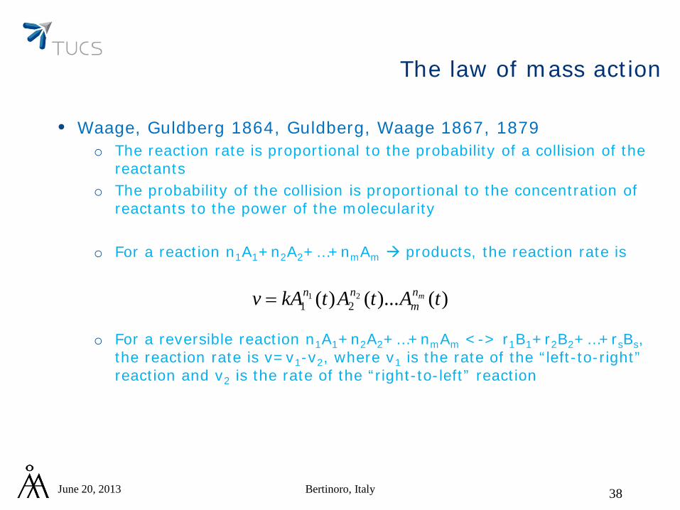
• Waage, Guldberg 1864, Guldberg, Waage 1867, 1879 o The reaction rate is proportional to the probability of a collision of the
reactants o The probability of the collision is proportional to the concentration of
reactants to the power of the molecularity
o For a reaction n1A1+n2A2+…+nmAm products, the reaction rate is
o For a reversible reaction n1A1+n2A2+…+nmAm <-> r1B1+r2B2+…+rsBs, the reaction rate is v=v1-v2, where v1 is the rate of the “left-to-right” reaction and v2 is the rate of the “right-to-left” reaction
June 20, 2013 Bertinoro, Italy
)()...()( 2121 tAtAtkAv mn
mnn=
39
Writing the mass-action ODE model
• The reaction rate gives the amount with which the concentration of every metabolite involved in the reaction changes per unit of time
o For a consumed metabolite, the change will be –v(t) o For a produced metabolite, the change will be v(t)
• Example
o For a reaction A->, the reaction rate is v(t)=kA(t)
dA/dt=-kA(T)
o For a reaction A+BC, the reactions rate is v(t)=kA(t)B(t), for some
constant k dA/dt=-kA(t)B(t), dB/dt=-kA(t)B(t), dC/dt=kA(t)B(t)
June 20, 2013 Bertinoro, Italy
June 20, 2013 Bertinoro, Italy 40
Coupled reactions
• Assume we have a set of reactions o A+B->C o A+2C<->B o C->2A
• Write the rates of all reactions
o v1=k1AB o v2=k2
+AC2-k2-B
o v3=k3C
• Write the differentials: for each metabolite, consider all reactions where it participates
o dA/dt=-v1-v2+2v3=-k1AB-k2+AC2+k2
-B+2k3C o dB/dt=-v1+v2=-k1AB+k2
+AC2-k2-B
o dC/dt=v1-2v2-v3=k1AB-2k2+AC2+2k2
-B-k3C
A predator-prey model
• A model where we have two species, one being the primary food source for the other
• Problem
o Whales, krill o Whales eat the krill; the krill live on the plankton in the sea o If whales eat too much krill, then the krill ceases to be abundant, and
the whales will starve or leave the area o As the population of whales declines, the population of krill increases o This makes the population of whales grow again, etc.
41 June 20, 2013 Bertinoro, Italy
A predator-prey model
• Assumptions and model formulation (the Lotka-Volterra model) o The krill population x(t), the whale population y(t) o The model as a reaction network
– Krill multiplies (assume infinite plankton as a food source for krill): X2X (a) – Whales eat krill: X+YY (b) – Whales die: Y (m) – Whales multiply only if there is krill: X+YX+2Y (n)
o The asociated mass-action ODE model: – dx/dt= ax(t)-bx(t)y(t) – dy/dt=-my(t)+nx(t)y(t)
o We have the model formulated as the system of the 2 ODEs
• Equilibrium points (or steady states) (xs,ys) o dx/dt=dy/dt=0 o (xs,ys)=(m/n,a/b) or (xs,ys)=(0,0)
42 June 20, 2013 Bertinoro, Italy
A predator-prey model: numerical integration
June 20, 2013 Bertinoro, Italy
0
50
100
150
200
250
300
350
1 59 117
175
233
291
349
407
465
523
581
639
697
755
813
871
929
987
1045
1103
1161
1219
1277
1335
1393
1451
1509
1567
1625
1683
1741
1799
1857
1915
1973
43
A predator-prey model: phase portrait
June 20, 2013 Bertinoro, Italy
0
50
100
150
200
250
300
350
0 20 40 60 80 100 120 140 160 180
44
Comments
• Mass-action kinetics leads to non-linear ODE models
• Even though non-linear, there is clear regularity in the structure of a mass-action ODE model
o Reactants consumed with the same rate as products are coming – The model is in fact linear in terms of reaction rates
o Well-specified form of the ODEs
– No longer have the option of obtaining a perfect fit by changing the form of the math model
– Can only fit the model through the kinetic rate constants – Fitting such models is a difficult problem
o Very different (easier!) to analyze an ODE system coming from a
mass-action reaction network than to analyze an arbitrary system of ODEs
June 20, 2013 Bertinoro, Italy 45
Kinetics of enzymatic reactions
June 20, 2013 Bertinoro, Italy 46
Enzymatic reactions
• Enzymes play a catalytic role in biology o Highly specific o Remain unchanged by the reaction o One enzyme molecule catalyzes about a thousand reactions per
second o Rate acceleration of about 106 to 1012-fold compared to uncatalyzed,
spontaneous reactions
• Enzymatic reactions usually described using more complicated models than mass-action
• Example: A is transformed into B through the help of enzyme E
o A+EB+E o Mass-action: dB/dt=kA(t)E(t) o Usual model for this reaction: dB/dt=vmaxA(t)/(KM+A(t))
• Discuss in the following the modeling of enzymatic reactions
June 20, 2013 Bertinoro, Italy 47
June 20, 2013 Bertinoro, Italy 48
Enzymatic reactions
• Brown (1902) proposed the following reaction model for irreversible enzymatic reactions: E+S <-> E:S -> E+P
• Michaelis, Menten (1913): assume that the first part of the reaction
is much faster than the second one: k1,k-1 >> k2
• Briggs, Haldane (1925): in some conditions, it may be assumed that E:S reaches quickly a steady state o This is the case if S(0)>>E (the enzyme is saturated by the substrate)
• Both assumptions lead to assuming that d(E:S)/dt=0, i.e., E:S is constant
o investigate what consequences this assumption has
• Frequently, the concentrations of several substances involved in biochemical reaction networks are included in so-called conservation sums.
• A characteristic feature of such substances is that they are neither produced nor degraded, however they can form complexes with other species or be part of other species.
55 June 20, 2013 Bertinoro, Italy
Mass conservation relations
• Example reactions: 2A ⇄ A2
A2 + B ⇄ A2:B A2:B → C + A2:B C → species: A, A2, B, A2:B, C - The total amounts of A and B are conserved in time. Neither of them
is produced nor degraded. 1×#A + 2×#A2 +2×#A2:B = const. 1×#B + 1×#A2:B = const.
56
−
−
−
−
=
1100
0010
0010
0011
0002
N
June 20, 2013 Bertinoro, Italy
Mass conservation relations
• To identify the conservation relations we solve the following equation in matrix G:
o Indeed, for such G:
• Example (continued):
57
0=GN
.0== GNvdtdSG
0GNGNS =
=
−
−−
−
=
=0110002021
11000010001000110002
CB:A
BAA
2
2
June 20, 2013 Bertinoro, Italy
Mass conservation relations
• The number of independent rows of G, i.e. the number of conservation relations, is equal to s-Rank(N).
o In the example s=5 and Rank(N)=3. It follows that G contains 2
independent rows, i.e., there are two mass conservation relations. o Observation: if the stoichiometric matrix has full rank, it follows that
the system has no conservation relations.
58 June 20, 2013 Bertinoro, Italy
Mass conservation relations
• Conservation relations can be used to reduce the system of differential equations dS/dt=Nv describing the dynamics of a reaction network.
• Each conservation relation leads to one more dependent variable, that can be expressed in terms of the independent variables and eliminated from the system of ODEs
• Always check the biological meaning of each mass conservation relation
59 June 20, 2013 Bertinoro, Italy
Steady states
June 20, 2013 Bertinoro, Italy 60
Steady state
• Steady state – one of the basic concepts of dynamical systems theory, extensively utilized in modelling. • Steady states (stationary states, fixed points, equilibrium points) are determined by the fact that the values of all state variables remain constant in time. • In steady state it holds for a reaction network that
• Solve the resulting algebraic equation in the unknowns S1,…,Ss (the s components of the steady state)
61 June 20, 2013 Bertinoro, Italy
𝑑𝑆𝑑𝑡 = 𝑁𝑁 = 0
Steady state
• Example (mass action kinetics) 2A → B (k1) A+B ⇄ C (k+
2,k-2)
Steady state algebraic equations ([A]0, [B]0, and [C]0 are unknowns) or
62
−⋅
−
−−
=
−+000
201
][][][
][
10
11
12
0
0
0
CkBAk
Ak
22
−=
+−=
+−−=
−+
−+
−+
02002
02002201
02002201
]C[k]B[]A[k0
]C[k]B[]A[k]A[k0
]C[k]B[]A[k]A[k20
N 0ν0
June 20, 2013 Bertinoro, Italy
Elementary fluxes
June 20, 2013 Bertinoro, Italy 63
Elementary flux modes
• Concept of elementary flux mode o a minimal set of enzymes (or, in other words, reactions) that can
operate at steady state o the smallest sub-networks that allow a bionetwork to function at
steady state o a minimal combination of reactions whose combined effect maintains
the network in steady state – any subset of it does not maintain the steady state
o they offer a key insight into the objectives of the network o each elementary flux mode should have a clear biological
interpretation in terms of the objectives of the network o determines whether a given set of enzymes/reactions are feasible at
steady states • Larger flux modes can be obtained by composing several flux modes: steady-state flux distributions
June 20, 2013 Bertinoro, Italy 64
Calculating the elementary flux modes
• We are interested in combinations of reactions whose combined effect is to preserve the steady state
o denote wi the weight of reaction i in the flux mode
o Recall: 𝑑𝑆𝑑𝑡
= 𝑁𝑁, where N is the stoichiometric matrix and v is the vector of fluxes
o We are interested in combinations of fluxes (w1,…,wr) that ensure 𝑑𝑆𝑑𝑡
= 0
o In other words, solve the equation Nw=0 in the unknown w o The solution is the kernel (or the null space) of matrix N
June 20, 2013 Bertinoro, Italy 65
Example
• Stoichiometric matrix: 1 −1 0 −10 2 −1 00 0 0 1
• NK=0 yields solution 𝐾 = 1 1 2 0
• In other words, in any steady state:
o The rates of production and degradation of S3 must be equal: v4=0 o v1+v2+2v3=0
June 20, 2013 Bertinoro, Italy 66
S1 2S2 S3
v1 v2 v3
v4
5. MODELS AND DATA
June 20, 2013 Bertinoro, Italy 67
Sources of error in modeling
• Formulation errors o Result from errors in the model formulation o Significant variables were ignored o Interrelationships between variables were ignored or simplified o Relating the data to the model in the wrong way: see for example
reporter systems • Truncation errors
o Come from the math techniques used in building the model o For example, an infinite series expansion may be truncated to a
polynomial • Round-off errors
o Numerical errors coming from representing real numbers with finite precision
• Measurement errors o Imprecision in the collection of data o Physical limitations of the instruments o Human errors
68 June 20, 2013 Bertinoro, Italy
Model fitting
• Problem: given the model and the data, is there a set of numerical values for all unknown kinetic parameters such that the numerical prediction of the model is ”close” to the data?
• Several components
o Search for parameter values – an optimization / machine learning problem
o Compare two sets of parameter values – introduce a suitable score function
o Judge quality of the final model fit – introduce a measure of fit quality
June 20, 2013 Bertinoro, Italy 69
Comparing two sets of parameter values
• Methods for judging the fitness of a model / comparing two sets of parameter values
o Chebyshev criterion: minimize the largest absolute deviation
– Intuition: more weight given to the worst point
o Minimize the sum of absolute deviations – Intuition: tends to treat each data point equally and to average the
deviations
o Least-squares – Intuition: somewhat in-between – Widely used in practice
o ...
70 June 20, 2013 Bertinoro, Italy
Fit quality
• Various methods for defining the a quantitative measure for the quality of a model fit
o Here present just one, from Kuhnel et al, BMC Systems Biology (2008)
o Only one data set at a time o Gives a measure of the average deviation of the model prediction
from the experimental data, normalized by (the average of) the absolute values of the model prediction
o This measure of fit quality does not discriminate against models aiming to explain experimental data with large absolute values
o Let exp be the experimental data; m the number of experimental points
o Rule of thumb (Kuhnel et al): lower than 20% value for qual(exp) can be considered as a good fit
June 20, 2013 Bertinoro, Italy 71
%100___
___
(exp) ⋅=valuespredictedofmean
mdeviationssquaredofsum
qual
6. HEAT SHOCK RESPONSE
June 20, 2013 Bertinoro, Italy 72
June 20, 2013 Bertinoro, Italy
The modeling of the heat shock response
• Intense research on modeling the HSR in the last years o HSR is an ancient, very well-conserved regulatory network across
all eukaryotes; bacteria have a similar mechanism – Good candidate for deciphering the engineering principles of regulatory
networks
o Heat shock proteins are very potent chaperones (sometimes called the “master proteins” of the cell)
– Involved in a large number of regulatory processes
o Tempting for a biomodeling, SysBio project because it involves relatively few main actors (at least in a first, simplified presentation)
• A number of models have been proposed o Some of them do not model the 3 components above o Some of them include modeling artifacts
• Discuss here a new, simple molecular model and its mathematical analysis o Standard, text-book-like molecular reactions only
73
June 20, 2013 Bertinoro, Italy
Heat shock response: main actors
• Heat shock proteins (HSP) o Very potent chaperones o Main task: assist the refolding of misfolded proteins o Several types of them, we treat them all uniformly in our model with hsp70 as
base denominator • Heat shock elements (HSE)
o Several copies found upstream of the HSP-encoding gene, used for the transactivation of the HSP-encoding genes
o Treat uniformly all HSEs of all HSP-encoding genes • Heat shock factors (HSF)
o Proteins acting as transcription factors for the HSP-encoding gene o Trimerize, then bind to HSE to promote gene transcription o Treat uniformly all HSFs with HSF1 as base denominator
• Generic proteins o Consider them in two states: correctly folded and misfolded o Under elevated temperatures, proteins tend to misfold, exhibit their
hydrophobic cores, form aggregates, lead eventually to cell death (see Alzheimer, vCJ, and other diseases)
I. Petre et al. A simple mass-action model for the eukaryotic heat shock response, and its mathematical validation. Natural Computing (2011) 10:595-612
June 20, 2013 Bertinoro, Italy
The mass-action ODE model
77
Modeling of the heat-induced misfolding
Question: how do we model the heat-induced misfolding?
• What is the temperature-dependant protein misfolding rate per second?
Adapted from Pepper et al (1997), based on studies of Lepock (1989, 1992) on differential calorimetry
ϕT=(1-0.4/eT-37) x 1.4T-37 x 1.45 x 10-5 s-1
Formula valid for temperatures
between 37 and 45, gives a generic protein misfolding rate per second
June 20, 2013 Bertinoro, Italy 78
June 20, 2013 Bertinoro, Italy
Parameter estimation
• Data readily available for the goal: Kline, Morimoto (1997) – heat shock of HeLa cells at 42C for up to 4 hours, data on DNA binding (HSF3:HSE)
• Requirements for the model: o 17 independent parameters, 10 initial values to estimate o 3 conservation relations available o The model must be in steady state at 37C, which gives 7 more algebraic
equations (each of them quadratic) o Altogether: 17 independent values
o Other conditions: total HSF somewhat low, refolding a fast reaction, HSPs long-
lived proteins
79
June 20, 2013 Bertinoro, Italy
The modeling/simulation environment
• Our choice: COPASI (www.copasi.org)
o Hoops, S., Sahle, S., Gauges, R., Lee, C., Pahle, J., Simus, N., Singhal, M., Xu, L., Mendes, P., and Kummer, U. (2006). COPASI — a COmplex PAthway SImulator. Bioinformatics 22, 3067-74.
o User-friendly o Stochastic and deterministic time course simulation o Steady state analysis o Metabolic control analysis o Mass conservation analysis o Optimization of arbitrary objective functions o SBML-based
o Excellent for parameter estimation o FREE!
80
June 20, 2013 Bertinoro, Italy
Parameter estimation
• Standard estimation procedure in COPASI (and not only) o Give the data and the target function o Give the list of parameters o The software scans the range of parameters and makes choices; for
each choice it evaluates the target function against the experimental data (least mean squares)
– The way it scans the space of parameter values depends on the chosen method
– Many sophisticated methods currently available – All are local-optimization methods
o It reports the best set of values
• Estimation repeated over and over again, with various methods for scanning the parameter space, to improve on the score of the fit
81
June 20, 2013 Bertinoro, Italy
Parameter estimation
• Model fit is anecdotically easy: “with a few free parameters, an elephant can always be fit”!
o Seems to come from a well known fact that for any given n points in the bi-dimensional space, a polynomial of suitable degree may be found to go through those points
o In practice, the polynomial cannot be chosen freely
• Our problem: o Find suitable parameter values and suitable initial values for all
variables so that the numerical prediction for [HSF3:HSE] is close to the experimental data of Kline-Morimoto (1997)
– Outcome: sure enough, “relatively easy” to find! o Additional requirement: the model must be in steady state at 37C
– This is a condition on the initial numerical values of the model – Difficulty: the values found as a good fit at 42C may not satisfy the
steady state condition! – Difficulty: to give this condition as a constrain to the model fit, one has
to solve analytically an algebraic system of large degree: impossible!
82
June 20, 2013 Bertinoro, Italy
Parameter estimation
• Solution: rather than solving the algebraic system, we look for an approximation of its solution: translate this condition into a more extensive model fit
o Problem: After obtaining the fit, the model is still not in the steady state!
o Solution: replace the estimated initial values with (the numerical estimations of) the steady state at 37C. Then the resulting system remains in the steady state at 37C
o Problem: The numerical fit (in absolute values) at 42C is ruined o Solution: recall that the Kline-Morimoto data is relative! In relative
terms, the fit is excellent!
83
June 20, 2013 Bertinoro, Italy
Parameter fit
84
I. Petre et al. A simple mass-action model for the eukaryotic heat shock response, and its mathematical validation. Natural Computing (2011) 10:595-612
June 20, 2013 Bertinoro, Italy
Predictions and validation 1. HSF dimers are only a
transient state between monomers and trimers The model however does not
ignore them because of kinetic considerations
Numerical simulations predict low levels of HSF dimers
2. Higher the temperature,
higher the response
3. Prolonged transcription at 43C confirmed Unlike previous models
4. Heat shock removed at the peak of the response confirms a more rapid attenuation phase
All data is in relative terms with respect to the highest value in the graph so that it can be easily compared
85
June 20, 2013 Bertinoro, Italy
Predictions and validation Experiment: two waves of heat
shock, the second applied after the level of HSP has peaked
Observation: the second heat shock response much milder than the first
• The reason is that the cell is better prepared to deal with the second heat shock
• Therapeutic consequences have been suggested: “train” the cell for heat shock by an initial milder heat shock
The model prediction is in line
with the experimental observation • Dotted line: heat shock at 42C for
two hours, behavior followed up to 20 hours
• Continuous line: heat shock at 42C for two hours, followed by a second wave of heat shock after the level of HSP has peaked
86
Model identifiability
• Problem: is there a unique set of parameter values that gives a “good” fit to the experimental data and validates all the additional tests? • Re-run the parameter estimation procedure
o use different initial values o use different (types of) machine learning methods
• Results o We obtained 10 more sets of parameter values that fit the
experimental data of Kline-Morimoto and keep the model in steady state at 37C
o All sets failed the model validation tests
June 20, 2013 Bertinoro, Italy 87
Model identifiability – systematic sampling of the parameter space
• Different approach: systematic sampling of the parameter space
o partition the domain of each parameter into a large number of subintervals (say 100.000); sample values for that parameter from each subinterval
o check the behavior of the model for all combinations of parameter values to get a sampling of the model behavior throughout the multi-dimensional parameter space
o Major problem: combinatorial explosion of the number of model variants
June 20, 2013 Bertinoro, Italy 88
Model identifiability – Latin Hypercube sampling
• Problem: huge number of samples to consider – (105)17=1085
• Fast, practical solution: the Latin Hypercube Sampling method (McKay, 1979)
– it provides samples which are uniformly distributed over each parameter – the number of samples is independent of the number of parameters – choose the size N of the sample; let p be the number of parameters – divide the domain of each parameter into N subintervals; randomly select
N numerical values for each parameter i, one from each of its subintervals; place the values on column i of a matrix Nxp
June 20, 2013 Bertinoro, Italy 89
Latin Hypercube sampling
June 20, 2013 Bertinoro, Italy 90
Insert here the sampled values for parameter i
Shuffle the values on each column
Read from here the sample values of the parameter set
Model identifiability – Latin Hypercube sampling
June 20, 2013 Bertinoro, Italy 91
I. Petre et al. A simple mass-action model for the eukaryotic heat shock response, and its mathematical validation. Natural Computing (2011) 10:595-612
Model identifiability – Latin Hypercube sampling
June 20, 2013 Bertinoro, Italy 92
I. Petre et al. A simple mass-action model for the eukaryotic heat shock response, and its mathematical validation. Natural Computing (2011) 10:595-612
Model identifiability
• Conclusion o likely that a model of this size is not uniquely identifiable o finding an optimal (or at least a “good”) model setup is very difficult
June 20, 2013 Bertinoro, Italy 93
7. DISCUSSION
June 20, 2013 Bertinoro, Italy 94
June 20, 2013 Bertinoro, Italy 95
Biomodeling with differential equations: some physical difficulties
•Assumes that the time evolution of a chemically reacting system is both continuous and deterministic •Difficulties with this assumption
o the time evolution is NOT continuous: molecular population levels increase and discrete only with discrete amounts
o the time evolution is NOT deterministic (even when ignoring the quantum effects and assuming classical mechanics for the molecular kinetics)
– it is only deterministic in the full position-momentum phase space (knowing the positions and velocities of all molecules)
– it is not deterministic in the N-dimensional space of the species population numbers
•However: o in many cases the time evolution of a chemical system can be treated
as continuous and deterministic o the difficulties come when some species populations are small, or in
conditions of chemical instability o Solution in these cases: stochastic models!
June 20, 2013 Bertinoro, Italy 96
Deterministic and stochastic modeling
Stochastic model • Given the current state of
the system, many possible future behavior are possible
• Probability distributions dictate the behavior of the system
• Well-suited to model individual, rather than average behavior
• Typical – Number of molecules are
modeled – Reactions are taking place
following “collisions” among the reactants
– Markov processes
Deterministic model • Given the current state of
the system, all future behavior of the system is uniquely defined
• Usually the model reflects the average behavior of the observed system
• Typical methods used: differential or difference equations
• Typical: – Concentrations of
molecules are modeled – Reactions are taking place
diffusion-like (gradient-like)
– Differential equations
June 20, 2013 Bertinoro, Italy 97
Deterministic and stochastic modeling
Stochastic modeling • The objects
– the number of copies of all species of interest
– the rates of all reactions • Main assumptions
– The system is well-stirred – The system is at
thermodynamical equilibrium • Methods
– Those of probability theory
ODE modeling • The objects
– the concentrations of all species of interest
– the rates of all reactions • Main assumptions
– The system is well-stirred – The system is at
thermodynamical equilibrium
• Methods – Those of mathematical
analysis (continuous mathematics)
June 20, 2013 Bertinoro, Italy 98
Deterministic and stochastic modeling
Stochastic model • It is the description of a
continuous time, discrete state Markov process
• Grand probability function: P(X1,X2,…,Xn,t) is the probability that at time t there are X1 molecules of species S1, …, Xn molecules of species Sn
• The grand probability function may be obtained through a differential equation: the chemical master equation
– Reason what is the probability of being in a certain state after one step
ODE modeling • The reaction rate gives the
amount with which the concentration of every metabolite involved in the reaction changes per unit of time
– For a consumed metabolite, the change will be –v(t)
– For a produced metabolite, the change will be v(t)
June 20, 2013 Bertinoro, Italy 99
Deterministic and stochastic modeling
Deterministic approach 1. based on the concept of
diffusion-like reactions 2. the time evolution of the
system is a continuous, entirely predictable process
3. governed by a set of ODEs 4. The system of ODEs is often
impossible to solve 5. it models the average behavior
of the system 6. assumes that the system is
well-stirred and at thermodynamical equilibrium
7. conceptual difficulties when small populations are involved
8. numerical simulations are straightforward and fast
9. impossible to reason about individual runs rather than the average
Stochastic approach 1. based on the concept of
reactive molecular collisions 2. the time evolution of the
system is a random-walk process through the possible states
3. governed by a single differential equation: the chemical master equation
4. the CME is often impossible to solve
5. it models individual runs of the system
6. assumes that the system is well-stirred and at thermodynamical equilibrium
7. no difficulties with small populations
8. numerical simulations via Gillespie’s SSA are slow
9. only gives individual runs; estimate the average through many runs
June 20, 2013 Bertinoro, Italy
Contributors
Collaborators on the heat shock response
• Computer Science and Math – Eugen Czeizler (Helsinki) – Vladimir Rogojin (Helsinki) – Elena Czeizler (Turku) – Andrzej Mizera (Turku) – Bogdan Iancu (Turku) – Diana-Elena Gratie (Turku) – Ralph Back (Turku)
• Biology and biochemistry
– John Eriksson (Turku) – Lea Sistonen (Turku) – Richard Morimoto (Chicago) – Andrey Mikhailov (Turku) – Claire Hyder (Turku)
Review paper together with • Diana-Elena Gratie (Turku,
Finland) • Bogdan Iancu (Turku, Finland)
Work funded by • Academy of Finland • Turku Centre for Computer Science • Centre for International Mobility