14
Computational statistics, lecture3 Resampling and the bootstrap Generating random processes The bootstrap Some examples of bootstrap techniques
| Date post: | 13-Dec-2015 |
| Category: |
Documents |
| Upload: | samantha-francine-foster |
| View: | 252 times |
| Download: | 2 times |
Computational statistics, lecture3
Resampling and the bootstrap
Generating random processes
The bootstrap
Some examples of bootstrap techniques

Computational statistics, lecture3
Process-based model of the flow of nitrogenfrom land to sea
CoastalmodelAnthropo-
genicinputs
Primary outputs(nutrient concentrations,chlorophyll, oxygen, etc.)
Open-seaboundaryconditions
Watershedmodel
Physio-graphicinputs
Meteoro-logical
forcings
Atmos-pheric inputs
Physio-graphicinputs
Waterborne inputs
Derived outputs
Meteoro-logical
forcings

Computational statistics, lecture3
Decomposing outputs of process-based modelsdriven by meteorological inputs
Observed forcing Weather-dependent model output
Synthetic forcing Synthetic model output
Weather-normalisedmean output
Weather-specific(random)
component of the model output
0
2
4
6
8
10
12
14
16
1 9 17 25 33 41 49 57 65 73 81 89 97 105 113
0
2
4
6
8
10
12
14
16
1 9 17 25 33 41 49 57 65 73 81 89 97 105 1130
2
4
6
8
10
12
14
16
1 9 17 25 33 41 49 57 65 73 81 89 97 105 113
-8
-6
-4
-2
0
2
4
6
8
1 10 19 28 37 46 55 64 73 82 91 100 109 118
0
2
4
6
8
10
12
14
16
1 9 17 25 33 41 49 57 65 73 81 89 97 105 113
0
2
4
6
8
10
12
14
16
1 9 17 25 33 41 49 57 65 73 81 89 97 105 113
0
2
4
6
8
10
12
14
16
1 9 17 25 33 41 49 57 65 73 81 89 97 105 113
0
2
4
6
8
10
12
14
16
1 9 17 25 33 41 49 57 65 73 81 89 97 105 113
How can we use resampling to better understand model outputs?

Computational statistics, lecture3
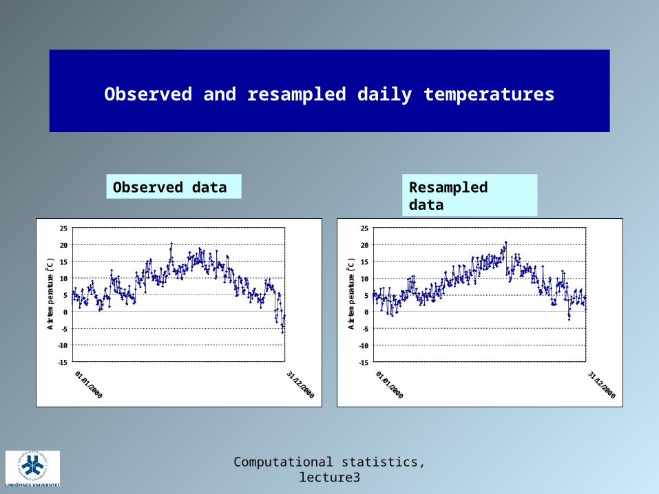
Resampling daily temperatures
Split observed data into periods of duration one month
Generate new temperature series by resampling 1-month pieces and combining them so that the seasonal pattern is preserved-15
-10
-5
0
5
10
15
20
25
01/01/1994
01/01/1995
01/01/1996
31/12/1996
31/12/1997
31/12/1998
31/12/1999
30/12/2000
Air
te
mp
era
ture
(oC
)
Computational statistics, lecture3
Observed and resampled daily temperatures
-15
-10
-5
0
5
10
15
20
25
01/01/2000
31/12/2000
Air
te
mp
era
ture
(oC
)
-15
-10
-5
0
5
10
15
20
25
01/01/2000
31/12/2000
Air
te
mp
era
ture
(oC
)
Observed data Resampled data
Computational statistics, lecture 3
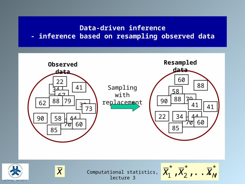
Data-driven inference- inference based on resampling observed data
**2
*1 ,...,, Nxxx
3467
798839
41
8570
62
90 58 4460
73
22
587988
41
88
8570
90
22 34 4460
41
60Sampling with replacement
Resampled dataObserved data
x **2
*1 ...,,, Nxxx

Computational statistics, lecture3
Nonparametric bootstrap - empirical cdf
0.00
0.20
0.40
0.60
0.80
1.00
1.20
0.00 1.00 2.00 3.00 4.00 5.00
Em
pir
ica
l cd
f (F
*)
n
ii xXI
nxF
1
)(1
)(*
Obs. nr Observed value1 0.572 0.083 0.204 0.355 0.726 0.107 0.648 4.269 3.07
10 1.2611 0.4912 0.1213 0.4514 2.9315 2.6016 0.1217 1.0118 2.9719 0.6120 1.64
Computational statistics, lecture3
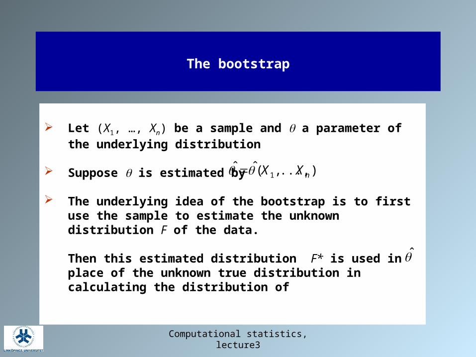
The bootstrap
Let (X1, …, Xn) be a sample and a parameter of the underlying distribution
Suppose is estimated by
The underlying idea of the bootstrap is to first use the sample to estimate the unknown distribution F of the data.
Then this estimated distribution F* is used in place of the unknown true distribution in calculating the distribution of
)...,,(ˆˆ1 nXX

Computational statistics, lecture3
Nonparametric bootstrap
- histogram of sample means of bootstrap samples
Obs. nr Observed value1 0.572 0.083 0.204 0.355 0.726 0.107 0.648 4.269 3.07
10 1.2611 0.4912 0.1213 0.4514 2.9315 2.6016 0.1217 1.0118 2.9719 0.6120 1.64
1.61.41.21.00.8
25
20
15
10
5
0
Sample mean
Fre
quency
Mean 1.237StDev 0.1937N 100
Histogram of Sample meanNormal

Computational statistics, lecture3
Nonparametric bootstrap
- histogram of sample means of bootstrap samples
Obs. nr Observed value1 0.572 0.083 0.204 0.355 0.726 0.107 0.648 4.269 3.07
10 1.2611 0.4912 0.1213 0.4514 2.9315 2.6016 0.1217 1.0118 2.9719 0.6120 1.64
2.241.961.681.401.120.840.56
600
500
400
300
200
100
0
Sample mean
Fre
quency
Histogram of bootstrap sample mean (B=10000)

Computational statistics, lecture3
Nonparametric bootstrap
- histogram of standard deviations of bootstrap samples
Obs. nr Observed value1 0.572 0.083 0.204 0.355 0.726 0.107 0.648 4.269 3.07
10 1.2611 0.4912 0.1213 0.4514 2.9315 2.6016 0.1217 1.0118 2.9719 0.6120 1.64
1.761.541.321.100.880.660.440.22
500
400
300
200
100
0
Sample st.dev.
Fre
quency
Histogram of bootstrap standard deviations
Computational statistics, lecture3
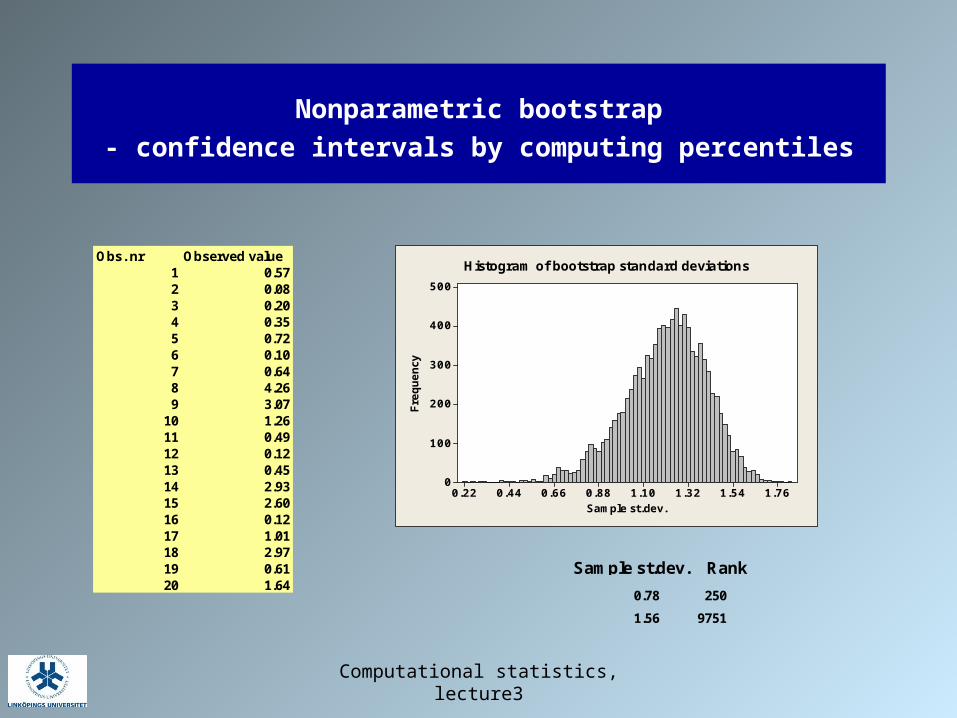
Nonparametric bootstrap
- confidence intervals by computing percentiles
Obs. nr Observed value1 0.572 0.083 0.204 0.355 0.726 0.107 0.648 4.269 3.07
10 1.2611 0.4912 0.1213 0.4514 2.9315 2.6016 0.1217 1.0118 2.9719 0.6120 1.64
1.761.541.321.100.880.660.440.22
500
400
300
200
100
0
Sample st.dev.
Fre
quency
Histogram of bootstrap standard deviations
Sample st.dev. Rank
0.78 250
1.56 9751

Computational statistics, lecture3
Parametric bootstrap - empirical cdf
Obs. nr Observed value1 0.572 0.083 0.204 0.355 0.726 0.107 0.648 4.269 3.07
10 1.2611 0.4912 0.1213 0.4514 2.9315 2.6016 0.1217 1.0118 2.9719 0.6120 1.64
Assume that a sample is drawn from an exponential distribution with cdf F(, x) = 1 – exp(- x)
Use the estimator
Determine the distribution of using the estimated distribution
X
1ˆ
),ˆ()(ˆ xFxF
Computational statistics, lecture3
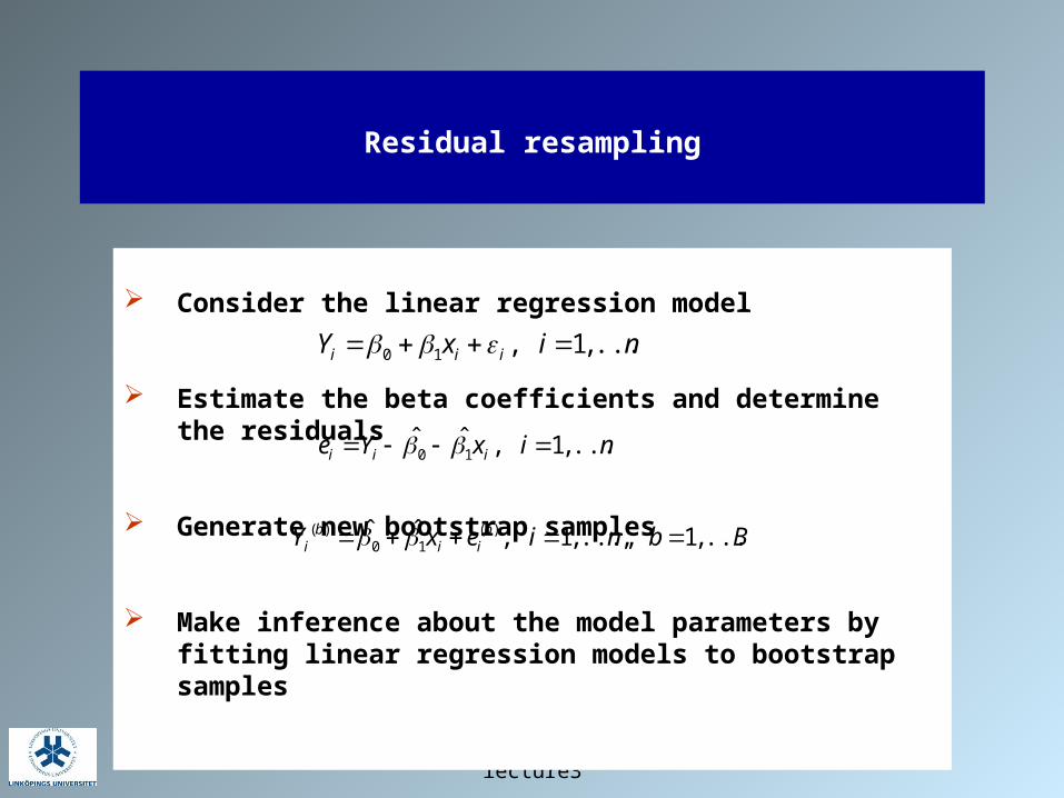
Residual resampling
Consider the linear regression model
Estimate the beta coefficients and determine the residuals
Generate new bootstrap samples
Make inference about the model parameters by fitting linear regression models to bootstrap samples
nixYe iii ...,,1,ˆˆ10
BbniexY bii
bi ...,,1,...,,1,ˆˆ )(
10)(
nixY iii ...,,1,10


