Computational Topology and Geometry: Supplementary …yap/classes/modeling/06f/lect/ll1.pdf ·...

Computational Topology and Geometry:

Supplementary Notes

Chee Yap

December 7, 2006

§1. Introduction and Course Mechanics

THIS is a document in progress, so you must be forgiving of mistakes. It is released under the beliefthat a flawed but timely document may be better than a perfect document that never sees the light of day.Please let me know of any errors!

I will add to this document throughout the course, so that we have only one document to deal with (thereare pluses and minuses). The main purpose is to supplement the references listed below.

The assigned homework will always be listed at the end of these notes.

Programming. This course addresses computational issues in computational topology and geometry. Assuch we will need to do some programming to better appreciate the computational issues.

You will work in groups of 2 (they call this ”extreme programming”) and I can testify that it makesprogramming a fun and social acitivity, on top of its educational/intellectual content. I want you to downloadour ”Core Library” from http://cs.nyu.edu/exact/ for doing your programming assignments.

If you live in a Windows environment, my best advice for using Core Library (and many other things!)is to download CYGWIN, a free Unix-like system that sits on top of Windows. Cygwin will have all thetools you need. For our course, I recommend these:

tar, Makefile,g++ compiler,

some keyboard-based text editor (VIM or GVIM, emacs, etc)

My webpage http://cs.nyu.edu/ yap/prog/ has basic information on CYGWIN, Make and other program-ming stuff. All serious programmers must learn a keyboard-based editor – I highly recommend GVIM (orVIM, the non-GUI version).

References. The basic references listed below will be augmented with papers and additional notes asneeded.

• Chapters from a forthcoming book, “Effective Computational Geometry for Curves and Surfaces”(Eds., J.-D.Boissonnat and M.Teillaud):A. Computational Topology: An Introduction, G.Rote and G.Vegter.B. Meshing of Surfaces, J.-D.Boissonnat, D.Cohen-Steiner, B.Mourrain, G.Rote, G.Vegter.

You will need to read each of these chapters; these files are downloadable from our class page.

• Geometry and Topology for Mesh Generation, by H.Edelsbrunner. Cambridge Press, 2001.

Mainly reference only.

c© Chee-Keng Yap December 7, 2006

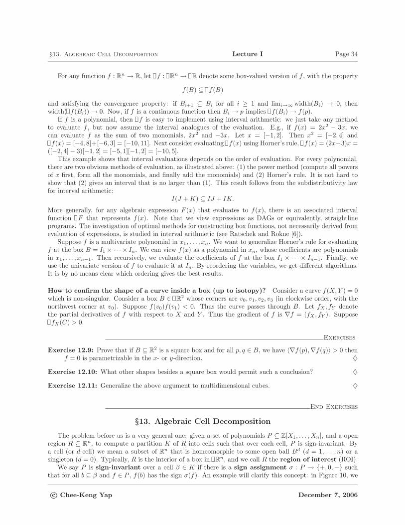
§2. Problems in Topological and Geometric Computation Lecture I Page 2

• Topology for Computing, by A.Zomorodian. Cambridge University Press, 2005.

Easy introduction to computational topology for computer scientists. Reference only.

• Robust Geometric Computation, by K.Mehlhorn and C.Yap.

Information about numerical-algebraic computation will be from this book manuscript, available frommy homepage.

• Fundamental Problems of Algorithmic Algebra, by C. Yap, Oxford Press 2000.

Mainly reference for algebraic computation. Available from my homepage.

Munkres [5] is an excellent additional reference for algebraic topology. A modern undergrad text (fromSpringer) by Christine Kinsey is very accessible.

§2. Problems in Topological and Geometric Computation

A main motivation for our subject is the computational aspect of the geometry and topology of curvesand surfaces. Such objects may be defined by its algebraic equation (e.g., S : F (X,Y,Z) = 0), or moreconstructively using some mesh with basis elements (e.g., B-splines), or perhaps by differential equations.We may wish to compute geometric properties of such objects (e.g., determine its location in space, or itscurvature at particular point, or its singularities). We may wish to determine topological invariants (e.g., itsBetti numbers, or determine if two paths on a surface are homotopic) which are global in nature.

The first step in any of the above tasks is to compute some more explicit, combinatorial, approximationof S from its defining equations or description. For example, from the equation F (X,Y,Z) = 0 of a surface,the basic properties of the surface are generally not obvious – where is it located in space, is it bounded, doesit have singularities? A more explicit representation such as a piecewise linear approximation of the surfacemay allow some of these questions to be answered more directly. You could display this approximation forvisual exploratoration of the surface. Visualization is an important tool for understanding geometric objects.

Such approximations are more generally called a cell complex. In applications, the cell complexes arepiecewise linear and are known as meshes. There are two main classes of meshes: surface mesh andvolume mesh, both embedded in 3-D. The computational task of converting a continuous characterizationof a geometric object into a discrete approximation is called meshing. We regard view meshing as thecritical step in the transition from continuous to discrete computation. If this step has error, any furthercomputations may be rendered invalid. We have described the typical transition, from continuous to discretebecause the continuous description is typically our starting point. But it is interesting to note that thereare situations where we seek to reverse this transition. For instance, given a 2-D mesh, we may want tofind a quadric surface that best approximates the mesh. Since the abstract continuous description is morecompact, this inverse meshing can be seen as a data compression problem.

Meshes are very diverse as they arises in many disciplines, such as engineering, physical simulation,geometric design and architecture. In mathematics, we may want to compute meshes (perhaps in highdimensions) to visualize a complicated geometry, or to use it for computing topological invariants. Whatwe call meshes are also known as “unstructured meshes”, as distinguished from “structured meshes” whosevertices come from a fixed grid (e.g., Z3). In recent years, considerable interest is attached to geometricobjects with even less structure than meshes: for instance, if we remove from the 2-dimensional cells from asurface mesh, we are left with a wire frame. If we further remove the 1-dimensional cells, we are left withonly the vertices. Such a set is called a point cloud. The reason for this interest is the availability ofnew sensing technology and devices which can easily produce such point cloud models of physical models.We now have another form of inverse meshing – how to construct a surface or volume mesh from the pointclouds?

The meshing problem thus encompasses a large variety of problems. We can initially classify themaccording to the nature of the input geometric description, and on the type of desired output mesh. Meshingcomputation involves a variety of numerical and algebraic techniques. We will briefly touch on some of these


§3. Historical Perspective Lecture I Page 3

techniques in this course. As a numerical computation, there are inevitable errors. So the big question inmeshing is how to guarantee the geometric and topology correctness despite such errors. Correctness criteria,of course, must be clearly specified. Minimally, the mesh should have the same topology, i.e., homeomorphicto the input object. But as an approximation, we also would like to guarantee metric properties, that themesh is close to the real geometry. Unfortunately, until recently, most published algorithms for meshinghave no guarantees.

We clarify our remark about the ways that meshing algorithms may go wrong. First, a meshing algorithmmay be using heuristics that are known to be incomplete (e.g., using Newton methods to search for zeros).A second source of error often escapes notice: even when the algorithm use provably correct methods, theymay still be inadequate. Typically, the correctness of such algorithms assumes an ideal computational modelwhere the numerical computation are error-free. But its implementation on a real computer may or may notintroduce serious difficulties. We are very interested in this transition from ideal to realistic computationalmodels. In recent years, much progress has been made in this direction. For instance, we now know alarge class of problems where the translation from the ideal model to an actual model can be automaticallyachieved by software.

Next, suppose we have obtained a correct mesh representation. On the geometric side, there is themesh refinement problem, i.e., to compute better approximations. This is usually an easier problemthan computing the very correct mesh. In the zero-dimensional case, meshing can be viewed as findingzeroes of a real function. Finding the correct initial mesh corresponds to the root isolation problem; meshrefinement amounts to the root refinement (which could be solved by a simple binary search). Concerningmesh refinement, there is an interesting representation of curves and surfaces based subdivision schemes.As the name suggests, the refinement strategy for such surfaces is built into the representation, i.e., apredefined subdivision method is used. However, the global aspects of such representations may be difficultto recover.

On the topological side, we usually have no need for further mesh refinement. We just need the appropriatetools from algebraic topology to compute the topological invariants from the mesh. In this course, we willlearn about some of these tools: homology, homotopy and Morse theory.

§3. Historical Perspective

The field of Computational Geometry started just over 30 years ago. For the most part, discrete compu-tational problems on linear objects (points, lines, hypersurfaces, polytopes, line arrangements, etc) were thefocus. In such a setting, the combinatorial aspects of computing dominates. An impressive set of algorithmicand analysis techniques have been developed over the last 30 years. In this course, we address the morerecent interest of Computational Geometry involving nonlinear geometry (curves and surfaces) where thedifficulties of continuous computation dominates. We will address the computational history of this topic inthree phases:

1. Traditionally, computational scientists and engineers use numerical approximations to compute withcurves and surfaces. The problem is that such methods are usually heuristic in nature. Such a numericalapproach is still the dominant practice.

2. There was a growing movement in academic circles in the last 20 years to counteract this practice.The idea is to replace numerical computation by algebraic (or symbolic) techniques. The advantage is clear– algebraic techniques are precise and error-free. But the problems of the algebraic approach also begin tomanifest themselves: such computations are too general (computes more than we really need) and are tooslow for many practical problems. It is not just a matter of trying to find faster algorithms – in many cases,the slowness is intrinsic. As an example, we can solve polynomial equations by reduction to computing withthe underlying ideals. This algebraic approach, however, captures more than just the geometry which isembedded in the radicals of the ideals. In a suitably general setting, computing with ideals requires double-exponential time, while the radical ideals is single-exponential time. Of course, even single-exponentialtime is not practical and so the search for special algorithms continues to be important in purely algebraicalgorithms. But this is still not sufficient.


§5. Review of Abelian Groups Lecture I Page 4

3. In recent years, another trend may be seen. That is the interest in combining algebraic with nu-merical techniques. This acknowledges the considerable merits of numerical techniques (namely it is fast),while rightly pointing out the need to make computations infallible, through a combination with algebraictechniques. For instance, the introduction of algebraic zero bounds with numerical approximation of roots(e.g., Core Library). This phase of development is still emerging. Although there are not many examples,we plan to look at some of these algorithms in this course.

Successful numerical-algebraic algorithms exhibit “adaptive” complexity. That means that the algo-rithms performs well for most inputs but not all; its complexity grows in proportion with its distance fromsingularities in the problem space. The challenge is how to quantify adaptivity.

§4. Review of Abelian Groups

The first part of our lectures is based on the chapter “Computational Topology: An Introduction” byVegter and Rote (part of a book [3] to appear). We suplement their chapter with details or extensions.

The chapter deals with two topological tools: homology and Morse theory. In particular, since homologyis defined through homomorphisms on Abelian groups, we must have some basic knowledge about Abeliangroups. We shall write groups additively, e.g., a group G may written more explicitly as (G,+, 0). All groupswill be Abelian. Note that an Abelian group G can be viewed as a Z-module where (n, g) 7→ ng.

If G,H are groups, a homomorphism is h : G → H such that h(x + y) = h(x) + h(y). If there is abijective homomorphism between G and H, then we say they are isomorphic and write G ≃ H.

Let S ⊆ G. Then the subgroup generated by S, denoted 〈S〉 is the set of all finite sums,

x =∑

gi∈S

nigi (1)

where ni ∈ Z. We call S a generator ofG if 〈S〉 = G. If S is a finite set, then we sayG is finitely generated.Our main goal is to give a constructive proof of the Fundamental theorem of finitely-generated Abeliangroups.

If S generates G with the additional property that each x ∈ G has a unique expression of the form (1),then S is a basis of G. If G has a basis, then it is called a free group. The rank of a free group G is thenumber of elements in a basis of G.

Note that if G is free, then for all x ∈ G and n ∈ Z, the value nx 6= 0 for n 6= 0. But when nx = 0,then we say x is of finite order. The smallest n > 0 such that nx = 0 is called the order of x. The setT = {x ∈ G : nx = 0, (∃)n ∈ Z} is called the torsion subgroup of G. If T = {0}, then we say G is torsionfree.

Let G1, . . . , Gn are groups. Then their direct sum is the group denoted G = G1 ⊕ · · · ⊕Gn where theunderlying set is G = G1×· · ·×Gn (Cartesian product) and the group operation is componentwise-operation.If the Gi’s are Abelian, then so is G.

Lemma 1. If Hi is a subgroup of an Abelian group Gi, then

G1 ⊕G2

H1 ⊕H2≃

(G1

H1

)⊕

(G2

H2

).

We leave this proof for an exercise. This lemma clearly extends to direct products of n groups, G1 ⊕· · · ⊕Gn.

Corollary 2. If G = G1 ⊕G2 then G/G1 ≃ G2.

Exercises

Exercise 4.1: Prove Lemma 1. ♦


§5. Smith Normal Form Lecture I Page 5

Exercise 4.2: Show that if an Abelian group G is finitely generated and torsion-free, then it is free. Showthat Q is torsion-free but not free. Conclude that Q is not finitely generated. ♦

End Exercises

§5. Smith Normal Form

A key computational tool in finitely generated Abelian groups is the Smith Normal form. See [7, chap. 10]for more details about Smith Normal form. You can download this from my webpage.

Let A ∈ Zm×n be an integer matrix. We say A is in Smith Normal Form (SNF) if A is diagonal, andthese diagonal elements are a1, a2, . . . , amin(m,n), with the property that each ai ≥ 0 and

ai|ai+1

for all i.Note that n|0 for all n ∈ Z, and if 0|n then n = 0. This means that in SNF, any zero diagonal element

ai = 0 must appear later than any non-zero diagonal element aj > 0, i.e., i < j. Similar, any ai that is equalto 1 must appear before any other aj 6= 1, i.e., i < j.

The non-zero diagonal elements are called Smith invariants or invariant factors of A.

For example, A =

[2 6 46 1 0

]is ...

A matrix U ∈ Zm×m is said to be unimodular if detU = ±1. Elementary row operations are oneof the following:(Ci) multiply the ith row by −1,(Pij) permute the ith and jth rows,(Rij(c)) replace ith row by c times the jth row (where c ∈ Z and j 6= i).

Each of these operations on A can be represented by a unimodular matrix U ∈ Zm×m and the correspond-ing transformation of A is given by matrix multiplication UA. Such a matrix U corresponding to elementaryrow matrices are called elementary matrices. Thus the matrices corresponding to three elementary rowoperations are:

Ci =

266666664

1

. . .

−1

. . .

1

377777775

, Pij =

266666666666664

1

. . .

0 1

. . .

1 0

. . .

1

377777777777775

, Rij(c) =

266666666666664

1

. . .

1

. . .

c 1

. . .

1

377777777777775

.

The diagonal entries are all 1’s unless otherwise indicated. It is also known that every unimodularmatrices can be obtained as a product of elementary matrices. Two matrices A and B are row equivalent ifB = UA.

Similarly, elementary column operations can be obtained by multiplying A on the right by an elementarymatrix V ∈ Zn×n. By an elementary operation we mean an elementary row or elementary columnoperation.

Let δk(A) be the GCD of all the order k minors of A. In particular, δ1(A) is the GCD of all the entriesof A. Recall that by convention, GCD is non-negative. It is easy to see from the definition that

δk(A)|δk+1(A).

We have


§6. Smith Normal Form Lecture I Page 6

Theorem 3. Every matrix A can be reduced to SNF by a sequence of elementary operations.

Proof. Let A be an m× n integer matrix. For i = 1, 2, . . . ,min{m,n}, we perform PHASE i: inductivelyassume that there are no non-zeros off the diagonal in the first i− 1 rows and in the first i− 1 columns.1. If the ith row and ith column are all zero, we are done. Go to the next phase. Otherwise, move thesmallest non-zero element from ith row or ith column to ith diagonal position (at aii). Make aii positive. Inthe following, aii will always be non-negative and non-increasing; any operation that strictly decreases aii issaid to be “critical”.2. Using elementary column operations, we make each off-diagonal element in the ith row zero. By inductivehypothesis, aij 6= 0 implies j > i. To zero out aij , we subtract or add a multiple of column i from the columnj. We choose the multiple so that the new aij is non-negative but strictly smaller than aii. There are twocases: (a) The new aij is now zero. (b) The new aij is non-zero. In the latter case, we exchange columnsi and j, so that the minimum value of aii is reduced. Note that (a) or (b) cannot occur indefinitely often.Thus Step 2 must halt, and we go to Step 3.3. Now, all the off-diagonal elements in the ith row is zero. Again, by elementary row operations, we makeevery off-diagonal element in the ith column 0. First by a row exchange and possibly multplication by −1,we ensure that the aiith entry is positive and smallest in magnitude in its column. If this exchange causesthe ith row to have two non-zero entries, go back to Step 2. As long as there is some j > i with aji 6= 0, weadd or subtract a multiple of the ith row to row j to ensure 0 ≤ aji < aii. If aji = 0, we repeat this reductionfor other choices of j. If aji > 0, we exchange rows i and j. If this exchange makes row i have more thanone non-zero entry, we go back to Step 2. Note that we cannot go from Step 3 to Step 2 indefinitely oftensince each time this happens a11 decreases.4. Eventually the ith row and ith column has only its diagonal element non-zero. We exit if i = min{m,n},otherwise, proceed to phase i+ 1.

At the end of these phases, all non-zero entries are found along the diagonal of the matrix. We canassume these non-zero entries are positive. We can make the smallest one divide all the other entries. Ifwe do not succeed, we would have found a strictly smaller smallest non-zero entry. This cannot continueindefinitely. Thus, eventually, the smallest non-zero entry divides all the other entries. We move this entryto position a11, and proceed to ensure that the next smallest entry divides the remaining entries. When thisis done, we move it to position a22. This will eventually give us the SNF. Q.E.D.

The above algorithm is not meant to be efficient. There are efficient (polynomial time) algorithms forcomputing the smith invariants (see [Yap]). However, this is still fairly expensive operation.

Lemma 4.(i) Elementary operations preserve δk(A).(ii) Elementary operations preserve the rank and set of Smith invariants of A.

It follows that if S is the SNF of A and have invariant factos a1, . . . , ar (r is the rank), then δ1(S) = a1,δ2(S) = a1a2, etc. Since δi(A) are unique, it follows that a1, . . . , ar are unique.

Exercises

Exercise 5.1: Show that the algorithm used to prove the existence of SNF is exponential time. ♦

Exercise 5.2: (a) Implement in Core Library an algorithm for computing the SNF of a matrix A. Thealgorithm takes as input the matrix A and outputs unitary matrices U and V and S such that S = UAVis SNF.

Do not worry about efficiency. NOTE: there is a Core Extension (COREX) for Linear Algebra thathas matrices. Please use this. If necessary, extend the Core Extension

(b) Use your algorithm to compute the SNF of the matrix of ∂1 and ∂2 for the triangulation of S2

above. ♦


§6. Finitely Generated Abelian Groups Lecture I Page 7

End Exercises

§6. Finitely Generated Abelian Groups

The next fact is quite expected:

Lemma 5. If B is a subgroup of A and A is a free Abelian group then B is free and rank(B) ≤ rank(A).

As corollary, any subgroup B of Z is isomorphic to Z.

Homomorphisms between free Abelian Groups. Let

f : F → G

be a homomorphism between the are free Abelian groups F,G of ranks n and m, respectively.Let e = (e1, . . . , en) be an ordered basis for F and e′ = (e′1, . . . , e

′m) be an ordered basis for G. If

f(ej) =

n∑

i=1

λije′i (2)

for j = 1, . . . , n, then the matrixΛf := (λij) ∈ Zm×n

is called the matrix of f relative to the bases e, e′. Then we have the following basic facts:

Lemma 6.(i) The rank of imf is the column rank of Λf .(ii) The rank of ker f is n− rank(imf) (also called the nullity of Λf ).

Proof. (i) This follows from the fact that imf is generated by the columns of Λf . Of course, the columnrank is the same as the rank of Λf .(ii) This follows from the fact that rank(ker f) + rank(imf) = rank(F ). This is a generalization of the factthat, for vector spaces, dim(ker f) + dim(imf) = dim(F ). Q.E.D.

We introduce the useful “bar notation”: for any x ∈ F , denote by

x = (x1, . . . , xn)T ∈ Zn

the vector such that 〈x, e〉 =∑n

i=1 xiei = x. This bar notation is relative to the choice of an ordered basise. For instance, relative to e, each ei is the ith elementary vector (0, . . . , 0, 1, 0, . . . , 0)T with a 1 in the i-thposition but 0 everywhere else. Similarly, for y ∈ G, let y ∈ Zm such that 〈y, e′〉 = y.

Fact 1. Let Λf be the matrix of f (relative to some ordered basis e, e′). Then we have that for all x ∈ F ,

f(x) = Λfx.

Proof. It is sufficient to note that this lemma holds when x = ej is a basis element of e: this follows fromthe definition of Λf in (2). Q.E.D.

We prove a normal for the matrix of homomorphisms between free Abelian groups:

Theorem 7 (Standard Bases for homomorphisms). If F,G are free Abelian of ranks n and m, and

f : F → G

is a homomorphishm, then there exists ordered bases d,d′ for F and G such that the matrix Λ of f is inSNF. We call d,d′ the “standard bases” for f .


§6. Finitely Generated Abelian Groups Lecture I Page 8

Proof. Let A ∈ Zm×n be the matrix of h relative to some ordered based e, e′. Let

S = UAV

be the SNF of A where U, V are unimodular matrices. For x ∈ F , we have

h(x) = Ax = U−1SV −1x.

Note that the vectordi = V ei

denote the ith column of V . Let di = 〈di, e〉 be the corresponding element of F . Then d = (d1, . . . , dn) isan ordered basis for F .

Now,f(di) = Adi

= (U−1SV −1)(V ei)= U−1Sei (ei ∈ Zn)

= U−1e′i (e′i ∈ Zm)

= aid′i (ai is the ith Smith invariant)

where we define d′i = U−1e′i. In the fourth line of this derivation, we use the fact that ei is the ith elementary

vector in Zn, and this implies Sei is equal to e′i, the ith elementary in Zm.

Hence d′i is the i-th column of U−1. Moreover, the sequence d′ = (d′1, . . . , d′m) is an ordered basis for G.

This proves that the matrix of f relative to the defined bases d,d′ is S. Q.E.D.

The next theorem gives a canonical form for the generators of subgroups of a finitely generated freeAbelian group:

Theorem 8 (Standard Bases for Subgroups). Let F be free Abelian of rank n and R a subgroup of F . Thenthere is an ordered basis e = (e1, . . . , en) for F , and positive integers r and t1, . . . , tk such that

t1|t2| · · · |tk

and d = (t1e1, . . . , tkek, ek+1, . . . , er) is an ordered basis for R. We call e,d the “standard bases” for (F,R).

Proof. By a previous lemma, we know that R is free of rank r ≤ n. Let

j : R→ F

be the inclusion homomorphism. By our theorem on normal form for homomorphism, there exist orderedbases e = (e1, . . . , er) for R and e′ = (e′1, . . . , e

′n) for F , such that the matrix of j relative to these bases is

a matrix S in SNF.Since j is 1-1, S has no zero column. Let S = Diag(a1, . . . , ar) ∈ Zm×r. Hence j(ei) = aie

′i (i = 1, . . . , r).

But since j is 1-1, we have j(ai) = ai, and the set {a1e′1, . . . , are

′r} is a basis for R. Suppose k of the

elements a1, . . . , ar are greater than 1, then we can rename them to be t1, . . . , tk; the remaining r−k elementsare all 1’s. This gives the form desired by our theorem. Q.E.D.

Finally, we can prove:

Theorem 9 (Fundamental Theorem of Finitely Generated Abelian Groups). Let G be a finitely generatedAbelian group.(i) Then G = H ⊕ T where T is the torsion subgroup of G and H is a free.(ii) There are finite cyclic groups T1, . . . , Tk where Ti has order ti > 1 such that t1| · · · |tk and T = T1⊕· · ·⊕Tk

(iii) The rank of H and t1, . . . , tk are determined by G.


§7. Homology of Simplicial Complex Lecture I Page 9

Proof. Let S = {g1, . . . , gn} be a set of generators for G, and F be the free group with ordered basise = (e1, . . . , en) generated by S. Consider the homomorphism,

h : F → G

where h(ei) = gi. Then h is onto. Let R = ker(h). Applying the previous theorem, there are bases for R,Fsuch that F ≃ F1 ⊕ · · · ⊕ Fn and

R ≃ (t1F1 ⊕ · · · ⊕ tkFk)⊕ (Fk+1 ⊕ Fr).

But G ≃ F/R, and from Lemma 1,

G ≃ F/R = (F ≃ F1 ⊕ · · · ⊕ Fn)/(t1F1 ⊕ · · · ⊕ tkFk)⊕ (Fk+1 ⊕ Fr)

= (F1/t1 ⊕ · · · ⊕ Fk/tk)⊕ (Fr+1 ⊕ · · · ⊕ Fn).

We can take Ti = Fi/ti and H = Fn−r1 . Q.E.D.

REMARK: How can we can represent (“present”) finitely generated groups? Let G be an Abelian group.If S ⊆ G is a finite set of elements that generates G, and we are told about all relations about S, then wecan say that S is a presentation of G. Here is the formal way to describe this presentation. We are given anonto homomorphism

h : F → G

where F is the free group generated by S, and we are given a set of relations of S that characterize allrelations of kerh. The relations are just linear combinations of S that equal 0. The matrix Λ and its nullspace can equally be used to represent this information.

§7. Homology of Simplicial Complex

I want to slightly rewrite the definitions in Vegter/Rote.For d ≥ 0, let {v0, . . . , vd} be a set of affinely independent points in Rm. The convex hull of such a set is

called a simplex σ. To be precise, it is the closed set

σ := {d∑

i=0

civi : ci ≥ 0,

d∑

i=0

ci ≤ 1}.

Each vi is a vertex of σ, and let V (σ) = {v0, . . . , vd} denote the set of vertices. The dimension of σ isdim(σ) := |V (σ)| − 1; a d-dimensional simplex is also called a d-simplex. Sometimes, it is useful to regardas special case the simplex σ0 defined by the empty set, with no vertices: V (σ0) = ∅ (empty set) is allowed,and it has dimension −1. Hence, −1 ≤ dim(σ) ≤ m.

Each subset of V ′ ⊆ V (σ) defines a simplex τ ; we call τ a face of σ and denote this relation by “τ � σ”. If0 ≤ dim(τ) < dim(σ), then we call τ a proper face if σ. In the special cases of dim(τ) = 0, 1, 2, 3,dim(σ)−1we call τ a vertex, edge, triangle, tetrahedron and facet of σ.

This terminology is familiar from elementary geometry. In fact, as we define the remaining concepts, itwould be helpful for readers to keep in mind the example of a triangulation of a polygonal subset of theplane. Consider Figure 1(a). The first step in “algebraization” of topology is to introduce a direction toedges, and a clockwise/ counter clockwise order to triangles. In Figure 1(b), we arbitrarily directed eachedge from the smaller indexed vertex to the larger indexed vertex. Also, each triangle is arbitrarily giventhe counterclockwise direction.



0

1

2

3 4

5

7

8

9

13

16

6

15

14

12

10

11

(a) (b)

Figure 1: A Triangulation in the plane

Oriented Simplices. Given a simplex σ = {v0, . . . , vd}, an ordered simplex is the sequence of itsvertices, (vπ(0), . . . , vπ(d)) where π is a permutation on the index set {0, 1, . . . , d}. Two ordered simplices aresaid to be equivalent if their underlying permutations π and π′ differ by an even number of transpositions.This is an equivalence relations. Each equivalence classes is known an oriented simplex based on σ. Let[vπ(0), . . . , vπ(d)] denote the oriented simplex correspond to (vπ(0), . . . , vπ(d)).

Note that if dim(σ) > 0, then there are two equivalence classes. We arbitrarily choose an orientationclass as the positive orientaion, and the other (if any) is negative. If dim(σ) = 0, there is only oneequivalence class. If dim(σ) = −1, then σ has no equivalence classes.

Let [K]d denote the set of all oriented d-simplices of K. Also, let [K] =⋃

d≥0[K]d. A subset of B ⊆ [K] iscomplete if, for each simplex σ ∈ K, we choose exactly one oriented simplex based on σ. Call K, associatedwith such a complete set B, an oriented simplicial complex. The particular choice of B is not important,but we must be consistent in sticking through with our choice. For instance, in Figure 2(b), we depict asimplicial complex for the 2-sphere, and we choose for each 2-simplex an orientation (counterclockwise).When B is understood, then for σ ∈ K, we may write [σ] for the oriented simplex based on σ whichcorresponds to our choice B. It is sometimes convenient to let [σ]− denote the oppositely oriented simplexcorresponding to [σ]. Strictly speaking, the notation [σ]− is undefined when dim(σ) ≤ 0; but in the contextof simplicial chains, we can interpret [σ]− to be −[σ].

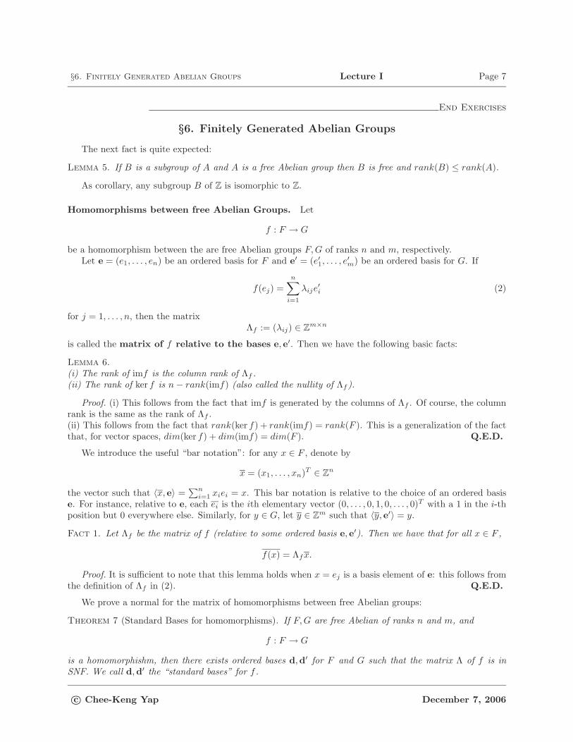
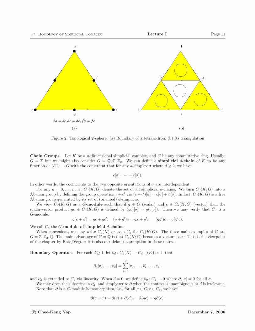
Compact, connected 2-manifolds. A primary source of examples of simplicial complexes will be 2-dimensional. So you must become familiar with the following basic examples: 2-sphere S2, torus T 2, Kleinbottle, real projective plane P2(R). These are all examples of connected, bounded 2-manifolds (S2 and T 2

are orientable surfaces, but Klein bottle and P2(R) are non-orientable).Every connected, bounded 2-manifolds can be topologically1 represented as a convex polygon whose

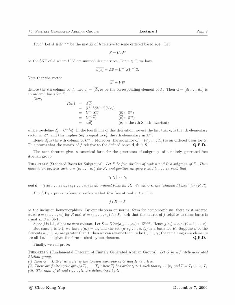
directed edges are identified in pairs. Conversely, every convex polygon whose directed edges are identifiedin pairs represents such a manifold. This is illustrated in Figure 2(a), where we draw a hexagon (a, b, c, d, e, f)where we identify the directed edges ba with bc, the directed edges dc with de, and the directed edges fa withfe. It easy to see that this really describes the boundary of a tetrahedron. After these identifications, we seethat the vertices a, c, e are the same vertex. Similarly, Figure 3(a) shows the polygonal representation of atorus, and Figure 3(b) is the polygonal representation of a Klein bottle. Because this is non-orientable, thissurface may be a little harder to understand (for instance, if we try to embed this surface in 2-dimensionalspace, it will self-intersect). Note that the four vertices of the rectangles in Figure 3 are identified: [a] =[b] = [c] = [d].

1I.e., up to homeomorphism.



b

d

f

c e

(a)

11

4

3

a

2

1

(b)

ba = bc, dc = de, fa = fe

Figure 2: Topological 2-sphere: (a) Boundary of a tetrahedron, (b) Its triangulation

Chain Groups. Let K be a n-dimensional simplicial complex, and G be any commutative ring. Usually,G = Z but we might also consider G = Q,C,Z2. We can define a simplicial d-chain of K to be anyfunction c : [K]d → G with the constraint that for any d-simplex σ where d ≥ 2, we have

c[σ]− = −(c[σ]).

In other words, the coefficients to the two opposite orientations of σ are interdependent.For any d = 0, . . . , n, let Cd(K;G) denote the set of all simplicial d-chains. We turn Cd(K;G) into a

Abelian group by defining the group operation c+ c′ via (c+ c′)[σ] = c[σ] + c′[σ]. In fact, Cd(K;G) is a freeAbelian group generated by its set of (oriented) d-simplices.

We view Cd(K;G) as a G-module such that if g ∈ G (scalar) and c ∈ Cd(K;G) (vector) then thescalar-vector product gc ∈ Cd(K;G) is defined by (gc)[σ] = g(c[σ]). Then we may verify that Cd is aG-module:

g(c+ c′) = gc+ gc′, (g + g′)c = gx+ g′x, (gg′)c = g(g′c).

We call Cd the G-module of simplicial d-chains.When convenient, we may write Cd(K) or even Cd for Cd(K;G). The three main examples of G are

G = Z,Z2,Q. The main advantage of G = Q is that Cd(K;G) becomes a vector space. This is the viewpointof the chapter by Rote/Vegter; it is also our default assumption in these notes.

Boundary Operator. For each d ≥ 1, let ∂d : Cd(K)→ Cd−1(K) such that

∂d[v0, . . . , vd] =

d∑

i=0

[v0, . . . , vi, . . . , vd].

and ∂d is extended to Cd via linearity. When d = 0, we define ∂0 : Cd → 0 where ∂0[σ] = 0 for all σ.We may drop the subscript in ∂d, and simply write ∂ when the context is unambiguous or d is irrelevant.Note that ∂ is a G-module homomorphism, i.e., for all g ∈ G, c ∈ Cp, we have

∂(c+ c′) = ∂(c) + ∂(c′), ∂(gc) = g∂(c).



b

de

e′

e

e

e

e′ e′ e′

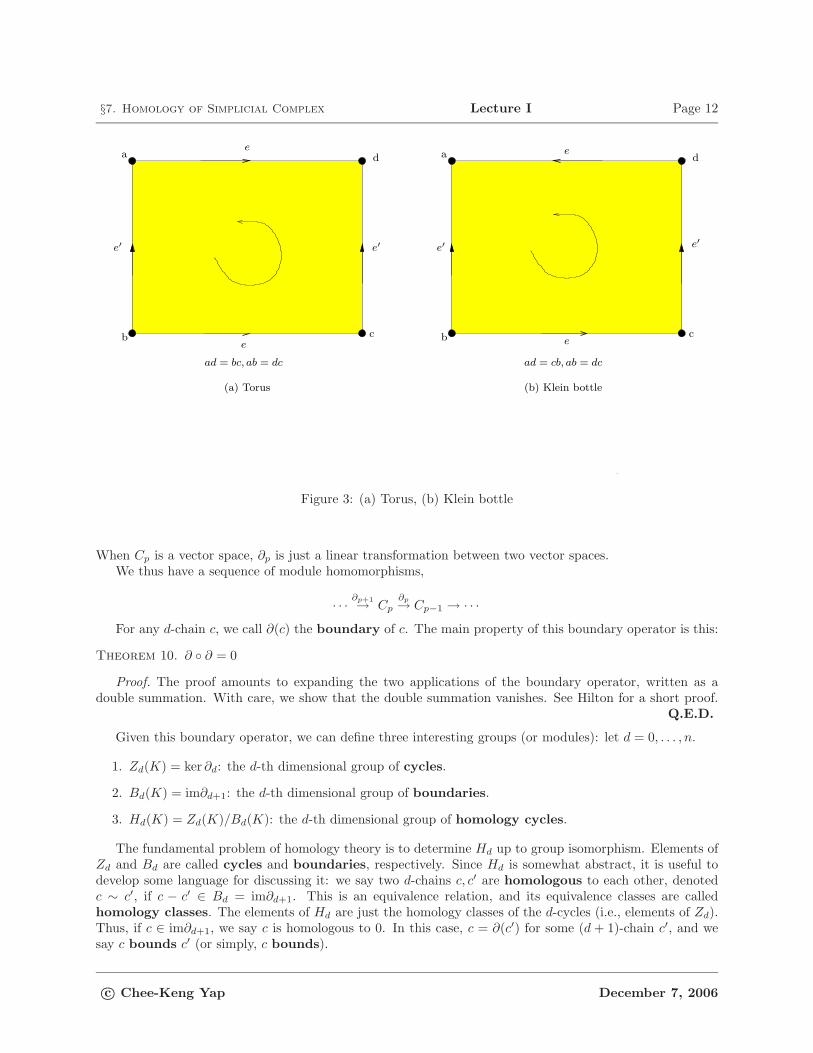
ad = bc, ab = dc ad = cb, ab = dc

(a) Torus (b) Klein bottle

a

cb

da

c

Figure 3: (a) Torus, (b) Klein bottle

When Cp is a vector space, ∂p is just a linear transformation between two vector spaces.We thus have a sequence of module homomorphisms,

· · · ∂p+1→ Cp∂p→ Cp−1 → · · ·

For any d-chain c, we call ∂(c) the boundary of c. The main property of this boundary operator is this:

Theorem 10. ∂ ◦ ∂ = 0

Proof. The proof amounts to expanding the two applications of the boundary operator, written as adouble summation. With care, we show that the double summation vanishes. See Hilton for a short proof.

Q.E.D.

Given this boundary operator, we can define three interesting groups (or modules): let d = 0, . . . , n.

1. Zd(K) = ker ∂d: the d-th dimensional group of cycles.

2. Bd(K) = im∂d+1: the d-th dimensional group of boundaries.

3. Hd(K) = Zd(K)/Bd(K): the d-th dimensional group of homology cycles.

The fundamental problem of homology theory is to determine Hd up to group isomorphism. Elements ofZd and Bd are called cycles and boundaries, respectively. Since Hd is somewhat abstract, it is useful todevelop some language for discussing it: we say two d-chains c, c′ are homologous to each other, denotedc ∼ c′, if c − c′ ∈ Bd = im∂d+1. This is an equivalence relation, and its equivalence classes are calledhomology classes. The elements of Hd are just the homology classes of the d-cycles (i.e., elements of Zd).Thus, if c ∈ im∂d+1, we say c is homologous to 0. In this case, c = ∂(c′) for some (d + 1)-chain c′, and wesay c bounds c′ (or simply, c bounds).



REMARK: We can be more abstract, by discarding all notions of geometric complexes (simplicial orotherwise), and simply study a ”chain complex” as a sequence

· · · ∂p+1→ Cp∂p→ Cp−1 → · · ·

of G-modules Cp and homomorphisms ∂p’s satisfying ∂p+1 ◦ ∂p = 0.

v3

v3

(a) (b)

v2

v1 v1

v0

v0v0

v2

v0

v4

v4

v6

v5

Figure 4: 7-vertex triangulation of the torus. (a) Bad (b) Good

Zero Dimensional Homology. For any simplicial complex K, its 0th homology group H0(K) is easyto describe: it is isomorphic to the group Zm where m is the number of connected components of the set|K|. Let us prove this. Let G = (V,E) be the undirected graph where V ⊆ K is the set of vertices in Kand E ⊆ K is the set of edges in K. The chain group C0(K) is generated by the set {[v1], . . . , [vk]}, whereV = {v1, . . . , vk}. Since ∂[vi] = 0 for all i, the cycle group Z0(K) is equal to C0(K).

We next determine the boundary group B0(K). Let G1, . . . , Gm be the subgraphs of G, correspondingto the m connected components of G. Choose a spanning tree Ti ⊆ E for each Gi. We may characterizeTi as a set of edges such that for every pair of vertices u, v ∈ Gi, there is a unique sequence path p(u, v) inTi from u to v. If e = (u, v), then ∂[e] = ∂[p(u, v)]. In other words, for all e ∈ E, there is a unique pathp(e) in some Ti such that ∂[e] = ∂[p(e)]. Let T = ∪m

i=1Ti. Since B0(K) is generated by {∂[e] : e ∈ E}, weconclude that it is in fact generated by {∂[e] : e ∈ T}. Pick a representative vertex ui in each Gi: so everyvertex in Gi is homologous to [ui]. Further, [ui] generates a free group isomorphic to Z. It follows that every0-chain in Gi is homologous to ni[ui] for some ni ∈ Z. Every 0-chain c ∈ C0(K) = Z0(K) can be uniquelydecomposed into c =

∑mi=1 ci where ci is an 0-chain in Gi. But each ci is homologous to some ni[ui]. Hence

c is homologous to∑m

i=1 ni[ui], a chain in the free group generated by {[u1], . . . , [um]}. So each element ofH0(K) is an equivalence class of the form

∑mi=1 ni[ui]. This proves that H0(K) is isomorphic to the free

Abelian group generated by [u1], . . . , [um], i.e., H0(K) ≃ Zm.

Homology of Euclidean Balls and Spheres. Besides compact 2-manifolds, the other main set of canon-ical examples from from Euclidean balls and spheres. Let us compute their homologies.

For n ≥ 1, let Bn = {p ∈ Rn : ‖p‖ < 1} denote the open unit n-ball. in Rn. Also let Bn

denote the

closure of Bn, and Bn = Bn \ Bn denote its boundary. We also call Bn the unit (n− 1)-sphere, denoted

Sn−1. For instance, B1 is the open interval (−1, 1) and S0 = {−1, 1}.



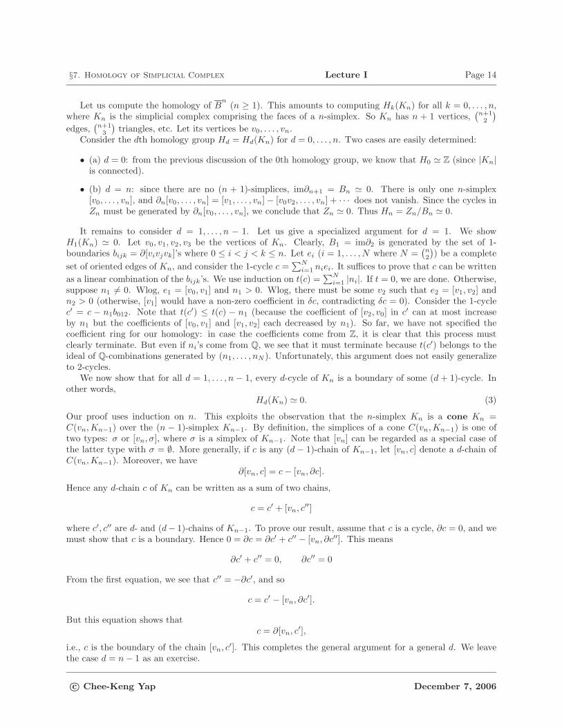
Let us compute the homology of Bn

(n ≥ 1). This amounts to computing Hk(Kn) for all k = 0, . . . , n,where Kn is the simplicial complex comprising the faces of a n-simplex. So Kn has n + 1 vertices,

(n+1

2

)

edges,(n+1

3

)triangles, etc. Let its vertices be v0, . . . , vn.

Consider the dth homology group Hd = Hd(Kn) for d = 0, . . . , n. Two cases are easily determined:

• (a) d = 0: from the previous discussion of the 0th homology group, we know that H0 ≃ Z (since |Kn|is connected).

• (b) d = n: since there are no (n + 1)-simplices, im∂n+1 = Bn ≃ 0. There is only one n-simplex[v0, . . . , vn], and ∂n[v0, . . . , vn] = [v1, . . . , vn]− [v0v2, . . . , vn] + · · · does not vanish. Since the cycles inZn must be generated by ∂n[v0, . . . , vn], we conclude that Zn ≃ 0. Thus Hn = Zn/Bn ≃ 0.

It remains to consider d = 1, . . . , n − 1. Let us give a specialized argument for d = 1. We showH1(Kn) ≃ 0. Let v0, v1, v2, v3 be the vertices of Kn. Clearly, B1 = im∂2 is generated by the set of 1-boundaries bijk = ∂[vivjvk]’s where 0 ≤ i < j < k ≤ n. Let ei (i = 1, . . . , N where N =

(n2

)) be a complete

set of oriented edges of Kn, and consider the 1-cycle c =∑N

i=1 niei. It suffices to prove that c can be written

as a linear combination of the bijk’s. We use induction on t(c) =∑N

i=1 |ni|. If t = 0, we are done. Otherwise,suppose n1 6= 0. Wlog, e1 = [v0, v1] and n1 > 0. Wlog, there must be some v2 such that e2 = [v1, v2] andn2 > 0 (otherwise, [v1] would have a non-zero coefficient in δc, contradicting δc = 0). Consider the 1-cyclec′ = c − n1b012. Note that t(c′) ≤ t(c) − n1 (because the coefficient of [v2, v0] in c′ can at most increaseby n1 but the coefficients of [v0, v1] and [v1, v2] each decreased by n1). So far, we have not specified thecoefficient ring for our homology: in case the coefficients come from Z, it is clear that this process mustclearly terminate. But even if ni’s come from Q, we see that it must terminate because t(c′) belongs to theideal of Q-combinations generated by (n1, . . . , nN ). Unfortunately, this argument does not easily generalizeto 2-cycles.

We now show that for all d = 1, . . . , n − 1, every d-cycle of Kn is a boundary of some (d + 1)-cycle. Inother words,

Hd(Kn) ≃ 0. (3)

Our proof uses induction on n. This exploits the observation that the n-simplex Kn is a cone Kn =C(vn,Kn−1) over the (n − 1)-simplex Kn−1. By definition, the simplices of a cone C(vn,Kn−1) is one oftwo types: σ or [vn, σ], where σ is a simplex of Kn−1. Note that [vn] can be regarded as a special case ofthe latter type with σ = ∅. More generally, if c is any (d − 1)-chain of Kn−1, let [vn, c] denote a d-chain ofC(vn,Kn−1). Moreover, we have

∂[vn, c] = c− [vn, ∂c].

Hence any d-chain c of Kn can be written as a sum of two chains,

c = c′ + [vn, c′′]

where c′, c′′ are d- and (d− 1)-chains of Kn−1. To prove our result, assume that c is a cycle, ∂c = 0, and wemust show that c is a boundary. Hence 0 = ∂c = ∂c′ + c′′ − [vn, ∂c

′′]. This means

∂c′ + c′′ = 0, ∂c′′ = 0

From the first equation, we see that c′′ = −∂c′, and so

c = c′ − [vn, ∂c′].

But this equation shows thatc = ∂[vn, c

′],

i.e., c is the boundary of the chain [vn, c′]. This completes the general argument for a general d. We leave

the case d = n− 1 as an exercise.



The following slick proof came up from the homework interviews with Gale Morehouse and MichaelBurr. Let us use the following elementary fact from the incremental Betti number algorithm: when you adda d-simplex to a complex, you either increase βd by 1 or decrement βd−1 by 1.

Thus, we have shown computed the Betti numbers of the Euclidean n-balls for all n ≥ 1 and d = 0, . . . , n:

βd(Bn) =

{1 if d = 00 else.

Building on this result, we next compute the homology of n-spheres Sn for n ≥ 0.First, assume n ≥ 1. Let ∂Kn+1 denote the triangulation obtained from Kn+1 by removing its sole

(n + 1)-simplex. Clearly, Sn is homeomorphic to the support∣∣∂Kn+1

∣∣. So Zd(∂Kn+1) = Zd(K

n+1) for alld = 0, . . . , n. Also Bd(∂K

n+1) = Bd(Kn+1) for all d = 0, . . . , n− 1, and Bn(∂Kn+1) = 0. Thus

Hd(∂Kn+1) = Hd(K

n+1)

for all d = 0, . . . , n − 1. Also, assuming the coefficient ring is Q, we see that Hn(∂Kn+1) ≃ Q sinceZn(∂Kn+1) ≃ Q and Bn(∂Kn+1) ≃ 0.

If n = 0, then S0 is just a pair of points, and clearly we have H0(S0) ∼ Z2.

Cell Complexes. Although simplicial complexes are easy to understand, their use in computating homol-ogy can be tedious (by hand) because we will need many simplices even for simple topological spaces. Forinstance, the smallest triangulation of the torus requires 7 vertices, 21 edges and 14 triangles. Computinghomology using a complex with so many cells is pushing the limits of casual hand computation. It turns outthat by generalizing simplicial complexes to “cell complex”, one can greatly reduce the number of cells, andbring many simple topological spaces within reach of hand computation.

Before defining the concept, let us see some natural examples of cell complexes. Figure 3 shows the cellcomplexes of the torus and Klein bottle. In each case, we begin with a rectangle complex: four vertices, fouredges and the interior of the rectangle (a 2-cell). Then we identify the opposite edges in pairs: dependingon how we do the identification, we get difference surfaces. Here, the torus and Klein bottle are indicated.After identification, we are left with a vertex v, two edges e, e′ and a 2-cell c. The set K = {v, e, e′, c} is ourthe cell complex.

b′

c′

a′

fC

e

d′

C

B2f

c

b = d

a

g

Figure 5: Cell Complex

A d-cell is any subset of Rn that is homeomorphic to of Bd (d ≥ 1); a 0-cell is just a singleton set. LetK be any non-empty finite collection of pairwise disjoint cells, where |K| = ∪K is a Hausdorff space. Butfor our purposes, we may assume |K| ⊆ Rn for some n. We call K a cell complex if, for each d-cell C ∈ K,

d ≥ 1, there is a continuous function fC : Bd → |K| such that fC is a homeomorphism from Bd onto C.

It can be shown that this implies that fC(Bd) is equal to a union of cells in K [5, p. 215]. NOTE: This isessentially the definition of CW-complex, except that we avoid the complications that arise in CW-complexwith infinitely many cells.

In Figure 5, we have K = {a, b, c, e, f, g, C} where a, b, c are 0-cells, e, f, g are 1-cells, and C is a 2-cell.

The map fC from B2

onto |K| (where f(a′) = a, f(b′) = b, etc) shows that K is a cell complex. Note that



fC is not a necessarily a homeomorphism of Bd

as seen in this example. When this extra condition is truefor every cell C, we call the cell complex regular.

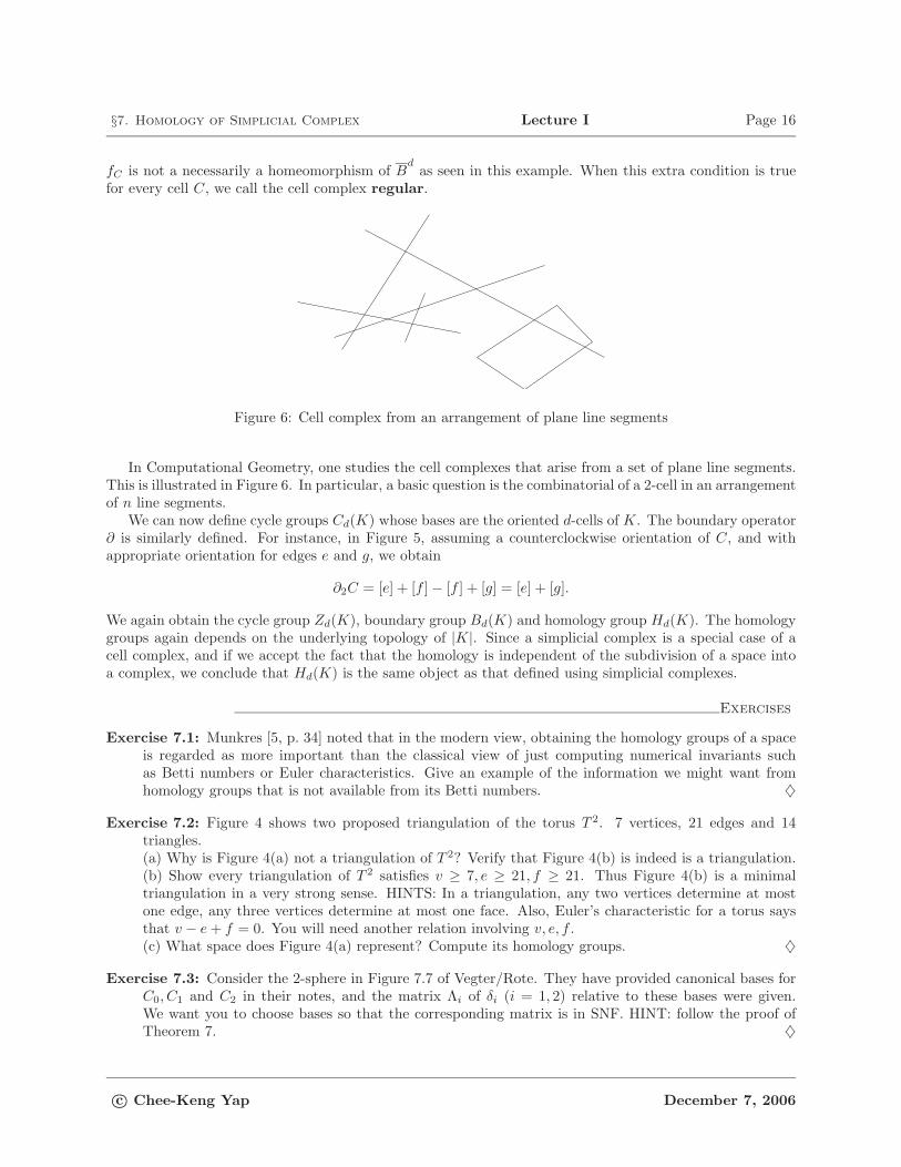
Figure 6: Cell complex from an arrangement of plane line segments

In Computational Geometry, one studies the cell complexes that arise from a set of plane line segments.This is illustrated in Figure 6. In particular, a basic question is the combinatorial of a 2-cell in an arrangementof n line segments.

We can now define cycle groups Cd(K) whose bases are the oriented d-cells of K. The boundary operator∂ is similarly defined. For instance, in Figure 5, assuming a counterclockwise orientation of C, and withappropriate orientation for edges e and g, we obtain

∂2C = [e] + [f ]− [f ] + [g] = [e] + [g].

We again obtain the cycle group Zd(K), boundary group Bd(K) and homology group Hd(K). The homologygroups again depends on the underlying topology of |K|. Since a simplicial complex is a special case of acell complex, and if we accept the fact that the homology is independent of the subdivision of a space intoa complex, we conclude that Hd(K) is the same object as that defined using simplicial complexes.

Exercises

Exercise 7.1: Munkres [5, p. 34] noted that in the modern view, obtaining the homology groups of a spaceis regarded as more important than the classical view of just computing numerical invariants suchas Betti numbers or Euler characteristics. Give an example of the information we might want fromhomology groups that is not available from its Betti numbers. ♦

Exercise 7.2: Figure 4 shows two proposed triangulation of the torus T 2. 7 vertices, 21 edges and 14triangles.(a) Why is Figure 4(a) not a triangulation of T 2? Verify that Figure 4(b) is indeed is a triangulation.(b) Show every triangulation of T 2 satisfies v ≥ 7, e ≥ 21, f ≥ 21. Thus Figure 4(b) is a minimaltriangulation in a very strong sense. HINTS: In a triangulation, any two vertices determine at mostone edge, any three vertices determine at most one face. Also, Euler’s characteristic for a torus saysthat v − e+ f = 0. You will need another relation involving v, e, f .(c) What space does Figure 4(a) represent? Compute its homology groups. ♦

Exercise 7.3: Consider the 2-sphere in Figure 7.7 of Vegter/Rote. They have provided canonical bases forC0, C1 and C2 in their notes, and the matrix Λi of δi (i = 1, 2) relative to these bases were given.We want you to choose bases so that the corresponding matrix is in SNF. HINT: follow the proof ofTheorem 7. ♦


§8. Effective Computation of Homology Lecture I Page 17

Exercise 7.4: Let K be a simplicial complex with n connected components. Then the group H0(K) is freeAbelian with basis given by a set S = {[σi] : i = 1, . . . , n}, where each connected component of |K| isrepresented by a unique vertex in S. ♦

Exercise 7.5: Most of our examples do not demonstrate torsion (in fact, all subspaces of Euclidean spacehas no torsion). To see how torsion arise, compute the homology groups of the Klein bottle. ♦

Exercise 7.6: Construct a space whose some homology group contains the torsion group Z3. HINT: considerhow Z2 arises in the Klein bottle. ♦

Exercise 7.7: (Relative Homology) Let L be a subcomplex of K. Then the chain groups Cp(L) are sub-groups of Cp(K). The quotient group Cp(K)/Cp(L) is called the group of relative chains of Kmodulo L, denoted Cp(K,L). Relative chain groups are free Abelian. Show that the boundaryoperator ∂ induces a homomorphism (still denoted ∂,

∂p : Cp(K,L)→ Cp−1(K,L).

We can then define the relative p-cycles and p-boundaries Zp(K,L), Bp(K,L) as before. The relativep-homology group is Zp(K,L)/Bp(K,L). ♦

Exercise 7.8: Give an algorithm to compute the Betti numbers of a simplicial complex K. ♦

End Exercises

§8. Effective Computation of Homology

It follows from the above considerations that Betti numbers of a simplicial complex K can be reduced toSNF computations.

It is best to illustrate the process with an example. Consider the triangulation of the 2-sphere (by atetrahedron) in Figure 2.

We see that the maps ∂1, ∂2 can be represented by

Λ(∂1) =

[12

]etc

Since SNF computation is expensive, and involves huge matrices for a large simplicial complex, we seekbetter methods. There is currently only a limited alterative, which we now present. This is an algorithmfrom Delfinado and Edelsbrunner [4] for computing Betti numbers of simplicial complexes in S3.

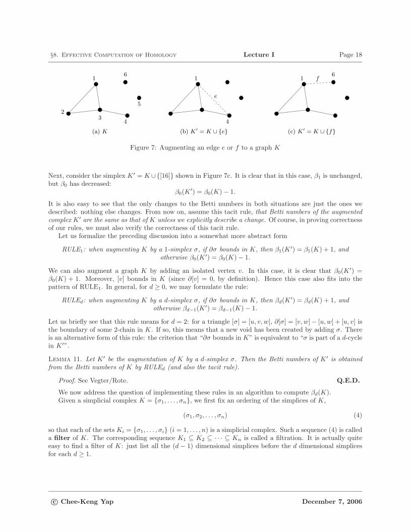
The basic idea is to use incremental construction of a simplicial complex K. Suppose σ 6∈ K andK ′ = K ∪ {σ} is also a simplicial complex. How does the Betti numbers of K ′ differ from that of K? Let ussee this in the simple case where K ′ is 1-dimensional i.e., K ′ is just a graph (see Figure 7).

Example: Incremental construction of a graph. Let K be the graph in Figure 7(a). We see thatβ0(K) = 3 (the number of connected components) and β1(K) = 1 (number of independent cycles). Supposewe augment K with an edge e = [14], as seen in Figure 7(b). How does this affect the first Betti numberβ1? Recall that that β1(K

′) is the number of independent 1-cycles in K ′ minus the number of independent1-boundaries. But the number of 1-boundaries is always 0 in a 1-dimensional complex (since there are no2-simplices). Note that K ′ now has 3 1-cycles, viz., [12]+[23]+[31], [13]+[34]+[41] and [12]+[23]+[34]+[41].But it is not hard to see that the number of independent 1-cycles in K ′ has increased by 1. Thus, weconclude that

β1(K′) = β1(K) + 1.


§8. Effective Computation of Homology Lecture I Page 18

(b) K′ = K ∪ {e} (c) K′ = K ∪ {f}

e

f1

23

4

5

61

4

16

(a) K

Figure 7: Augmenting an edge e or f to a graph K

Next, consider the simplex K ′ = K ∪{[16]} shown in Figure 7c. It is clear that in this case, β1 is unchanged,but β0 has decreased:

β0(K′) = β0(K)− 1.

It is also easy to see that the only changes to the Betti numbers in both situations are just the ones wedescribed: nothing else changes. From now on, assume this tacit rule, that Betti numbers of the augmentedcomplex K ′ are the same as that of K unless we explicitly describe a change. Of course, in proving correctnessof our rules, we must also verify the correctness of this tacit rule.

Let us formalize the preceding discussion into a somewhat more abstract form

RULE1: when augmenting K by a 1-simplex σ, if ∂σ bounds in K, then β1(K′) = β1(K) + 1, and

otherwise β0(K′) = β0(K)− 1.

We can also augment a graph K by adding an isolated vertex v. In this case, it is clear that β0(K′) =

β0(K) + 1. Moreover, [v] bounds in K (since ∂[v] = 0, by definition). Hence this case also fits into thepattern of RULE1. In general, for d ≥ 0, we may formulate the rule:

RULEd: when augmenting K by a d-simplex σ, if ∂σ bounds in K, then βd(K′) = βd(K) + 1, and

otherwise βd−1(K′) = βd−1(K)− 1.

Let us briefly see that this rule means for d = 2: for a triangle [σ] = [u, v, w], ∂[σ] = [v, w]− [u,w] + [u, v] isthe boundary of some 2-chain in K. If so, this means that a new void has been created by adding σ. Thereis an alternative form of this rule: the criterion that “∂σ bounds in K” is equivalent to “σ is part of a d-cyclein K ′”.

Lemma 11. Let K ′ be the augmentation of K by a d-simplex σ. Then the Betti numbers of K ′ is obtainedfrom the Betti numbers of K by RULEd (and also the tacit rule).

Proof. See Vegter/Rote. Q.E.D.

We now address the question of implementing these rules in an algorithm to compute βd(K).Given a simplicial complex K = {σ1, . . . , σn}, we first fix an ordering of the simplices of K,

(σ1, σ2, . . . , σn) (4)

so that each of the sets Ki = {σ1, . . . , σi} (i = 1, . . . , n) is a simplicial complex. Such a sequence (4) is calleda filter of K. The corresponding sequence K1 ⊆ K2 ⊆ · · · ⊆ Kn is called a filtration. It is actually quiteeasy to find a filter of K: just list all the (d − 1) dimensional simplices before the d dimensional simplicesfor each d ≥ 1.


§9. Euler Characteristic and Betti Numbers Lecture I Page 19

Union-Find Datastructure. The main computational task in implementing our RULE above is to de-termine, for given K and d-simplex σ, whether ∂σ bounds in K.

In case d = 1, the simplex σ is a directed edge [u, v]. Then ∂(σ) = [v]− [u] bounds in K iff u, v belongs tothe same connected component. This can be decided very efficiently by using a well-known data structure inComputer Science called the Union-Find data structure. In a certain (amortized) sense, each operation costsO(α(n)) where n is the total number of vertices in the eventual complex, and α(n) is a very slow growingfunction called the inverse Ackermann function.

There is no known computational technique for d = 2. However, if the dimension of K is 3, then wecan exploit duality: d-simplex in R3 is the same as a “dual (3 − d)-dimensional” simplex. In particular,2-simplices will be dual 1-simplex. So we can use the Union-Find data structure in the dual setting.

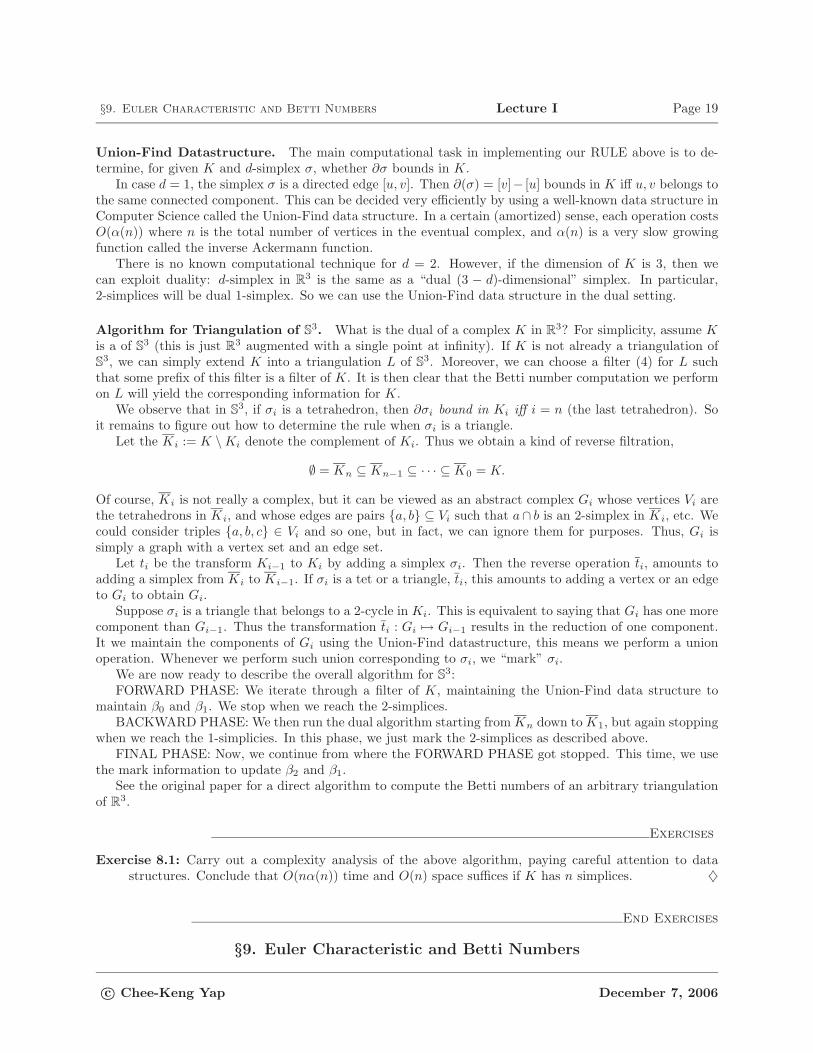
Algorithm for Triangulation of S3. What is the dual of a complex K in R3? For simplicity, assume Kis a of S3 (this is just R3 augmented with a single point at infinity). If K is not already a triangulation ofS3, we can simply extend K into a triangulation L of S3. Moreover, we can choose a filter (4) for L suchthat some prefix of this filter is a filter of K. It is then clear that the Betti number computation we performon L will yield the corresponding information for K.

We observe that in S3, if σi is a tetrahedron, then ∂σi bound in Ki iff i = n (the last tetrahedron). Soit remains to figure out how to determine the rule when σi is a triangle.

Let the Ki := K \Ki denote the complement of Ki. Thus we obtain a kind of reverse filtration,

∅ = Kn ⊆ Kn−1 ⊆ · · · ⊆ K0 = K.

Of course, Ki is not really a complex, but it can be viewed as an abstract complex Gi whose vertices Vi arethe tetrahedrons in Ki, and whose edges are pairs {a, b} ⊆ Vi such that a∩ b is an 2-simplex in Ki, etc. Wecould consider triples {a, b, c} ∈ Vi and so one, but in fact, we can ignore them for purposes. Thus, Gi issimply a graph with a vertex set and an edge set.

Let ti be the transform Ki−1 to Ki by adding a simplex σi. Then the reverse operation ti, amounts toadding a simplex from Ki to Ki−1. If σi is a tet or a triangle, ti, this amounts to adding a vertex or an edgeto Gi to obtain Gi.

Suppose σi is a triangle that belongs to a 2-cycle in Ki. This is equivalent to saying that Gi has one morecomponent than Gi−1. Thus the transformation ti : Gi 7→ Gi−1 results in the reduction of one component.It we maintain the components of Gi using the Union-Find datastructure, this means we perform a unionoperation. Whenever we perform such union corresponding to σi, we “mark” σi.

We are now ready to describe the overall algorithm for S3:FORWARD PHASE: We iterate through a filter of K, maintaining the Union-Find data structure to

maintain β0 and β1. We stop when we reach the 2-simplices.BACKWARD PHASE: We then run the dual algorithm starting from Kn down to K1, but again stopping

when we reach the 1-simplicies. In this phase, we just mark the 2-simplices as described above.FINAL PHASE: Now, we continue from where the FORWARD PHASE got stopped. This time, we use

the mark information to update β2 and β1.See the original paper for a direct algorithm to compute the Betti numbers of an arbitrary triangulation

of R3.

Exercises

Exercise 8.1: Carry out a complexity analysis of the above algorithm, paying careful attention to datastructures. Conclude that O(nα(n)) time and O(n) space suffices if K has n simplices. ♦

End Exercises

§9. Euler Characteristic and Betti Numbers


§11. Morse Theory Lecture I Page 20

The Euler Characteristic is an integer that can be associated to topological spaces; in fact, it can becomputed as the alternating sum of the Betti numbers. See the interesting account of Imre Lakatos in“Proofs and Refutations”, which traces historical development from the initial ideas of Euler to the algebraicview of Poincare that is our modern viewpoint. But even Poincare made a mistake and discovered torsion asa result. Lakatos’ point (as a historian of science) is that these definitions are subject to various forces akinto negotiations. But I think it is a serious lapse to think that these negotiations are arbitrary and purelypower play (as deconstructionists would have us believe). Massey [Chap.VI] also gives a brief historicalbackground of homology theory.

We begin with the original intuitive facts about Euler Characteristic of a space. The initial observationfrom Euler is that for a planar triangulation of a simply-connected planar region R, the following invariantholds:

v − e+ f = 2

where v, e, f is the number of vertices, edges, faces of the triangulation. It turns out that this number 2 doesnot depend on the choice of triangulation of R, – so we say the Euler characteristic for R is two, χ(R) = 2.We then generalize this to solid polyhedral objects, and so on. Eventually, we obtain the formula

χ(K) =

d∑

i=0

(−1)drank(Ci(K)).

This can be shown inductively. We can further relate this to the Betti numbers,

χ(K) =d∑

i=0

(−1)dβi(K).

[See Vegter-Rote].A basic result of homology theory is that the Betti numbers βi(K) depends only on the topology2 of the

underlying space |K|, not on the particular triangulation. We can also show that βi(K) is a homotopyinvariant: if |L| is homotopic to |K| then βi(L) = βi(K) [See Vegter-Rote].

The interpretation of Betti numbers in R3 is quite interesting:β0 is the number of connected components.β1 is the number of holes. E.g., a donut has one hole, and an eye-glass frame (typically) has two holes.β2 is the number of voids. E.g., a soccer ball has one void (which is filled with air). Biological cells can

be viewed as a medium filled with some fluid, with numerous voids containing a variety of material.Here is an application: suppose we are given a model of a very complex molecule, regarded as the union

of balls in R3 of various radii. Each ball corresponds to an atom (e.g., a hydrogen atom has a smaller radiusthan an oxygen atom). Since the biological functions of molecule often depends on the geometry of themolecules, there is interest in computing the number of holes and voids in such a molecute.

§10. Notes on Homotopy

Another way to get topological invariance is via homotopy. Again we algebraize the concept and discretizeit to obtain the group analogue of homology groups, called fundamental groups. The relative advantagesand disadvantages of using fundamental group invariants will become clear.

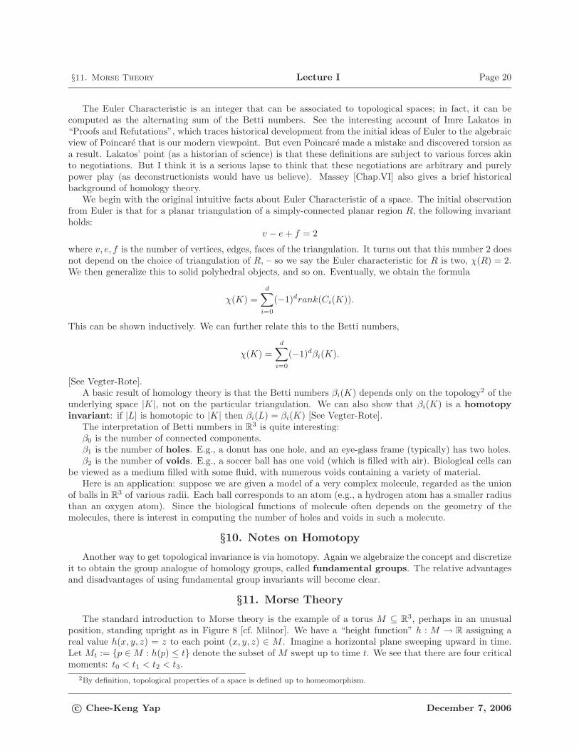
§11. Morse Theory

The standard introduction to Morse theory is the example of a torus M ⊆ R3, perhaps in an unusualposition, standing upright as in Figure 8 [cf. Milnor]. We have a “height function” h : M → R assigning areal value h(x, y, z) = z to each point (x, y, z) ∈ M . Imagine a horizontal plane sweeping upward in time.Let Mt := {p ∈M : h(p) ≤ t} denote the subset of M swept up to time t. We see that there are four criticalmoments: t0 < t1 < t2 < t3.

2By definition, topological properties of a space is defined up to homeomorphism.



t1

t3

t2

t0

Figure 8: Torus in an upright position

1. t < t0, when Mt is empty.

2. t = t0, when Mt is a single point.

3. t ∈ (t0, t1), when Mt is homeomorphic to a 2-cell.

4. t = t1, when the boundary of the 2-cell is just pinched.

5. t ∈ (t1, t2), when Mt is homeomorphic to a cylinder.

6. t = t2, when the boundary components of the cylinder first meets.

7. t ∈ (t2, t3), when Mt is homeomorphic to a torus with a puncture.

8. t > t3, when Mt is a torus T 2.

In terms of homotopy types,

1. At time t0, we attach a 0-cell to Mt.

2. At times t1 and t2, we attach a 1-cell to Mt,

3. At time t3, we attach a 2-cell to Mt.

It turns out that the height function h has four critical points p0, p1, p2, p3, where pi corresponds to thecritical moment ti. These points are, respectively, a minima, a saddle, a saddle and a maxima. Morse theoryassigns a natural number (“index”) to these critical points: in fact pi has index d iff we attach a d-cell toMt at time ti. Thus, the study of the critical points and the critical values ti of a smooth function h couldreveal information about topological changes in Mt, and ultimately about M itself.

In general, Morse theory studies topological invariants of smooth manifolds M ⊆ Rn as revealed bystudying critical points of smooth functions on M . Height functions are examples of Morse functions onM : such a function is defined to be a smooth function h : M → R whose critical points are nondegenerate.

The first part of this lecture is basically concerned with making the concepts in this definition precise.We will need to generalize familiar concepts in Euclidean space to arbitrary manifolds.

The Vegter/Rote treatment has the merit of simplifying definitions by considering only manifolds whichare embedded in Euclidean space.

It is helpful to keep two basic principles in mind throughout differential geometry (which provides thefoundation for Morse theory): Local Principle [L] and Euclidean Principle [E]. For instance, a manifold is



locally [L] like an Euclidean space [E]. The Euclidean Principle says that we map all concepts in abstractspaces back to Euclidean space. For instance, to define the concept of differentiable function f on manifolds,we first define differentiability at a point [L], and reduce differentiability of f to the differentiability of atransformed function f on Euclidean neighborhoods [E]. The Local Principle has a corollary: nonlinearphenomenon when localized becomes a linear phenomenon. Thus the local linear transformations (Jacobiansand tangent spaces, etc) becomes the key.

Smooth Manifolds. We say f : Rn → R is smooth if, for all n ≥ 0, the nth derivative f (n) exists. Afunction ϕ : Rn → Rm is smooth if each component fi of ϕ(x) = (f1(x), . . . , fn(x)) is smooth.

We need to introduce the differential of ϕ at q ∈ Rn: this is the linear map dϕq : Rn → Rm such thatfor all v ∈ Rn, and for all curves αv : (−ε, ε) → Rn given by αv(t) = ϕ(q + tv), we have dϕq(v) = α′

v(0)(where α′

v denotes differentiating αv(t) by t. Concretely, dϕq is a given by the m× n Jacobian matrix,

∂f1

∂x1(q) · · · ∂f1

∂xn(q)

.... . .

...∂fm

∂x1(q) · · · ∂fm

∂xn(q)

Note that dϕq is a constant matrix for each q. Alternatively, we can view dϕ as a map from Rn to lineartransformations from Rn to Rm.

f

Figure 9: Smooth Curves (picture) and Manifolds

Next, we want to define what it means for M ⊆ Rn to be a smooth manifold. Sometimes, one says“differentiable” or “C∞” instead of “smoothness”. By a diffeomorphism f : U → V (U, V ⊆ Rn) we meana smooth function whose inverse f−1 is defined and also a diffeomorphism. For instance f : R → R wheref(x) = x3 is a smooth homeomorphism function, but it is not a diffeomorphism because f−1 is not smoothat 0.

Let us first consider the special case: what is a smooth curve M embedded in R2? Applying the localprinciple [L], we say that the set M ⊆ R2 is a smooth curve at p ∈ M if there exists an open intervalU ⊆ R, an open set V ⊆ R2 such that p ∈ V and there exists a smooth function ϕ : U → R2 such that (1) ϕis a diffeomorphism from U to V ∩ S, and (2) dϕq 6= 0. We say M is a smooth curve if it is smooth at eachp ∈M .

More generally, M ⊆ Rn is a smooth m-fold if for all p ∈M , there exists an open set U ⊆ Rm, and openset V ⊆ Rn, such that for some smooth onto homeomorphism ϕ : U → M ∩ V such that dϕq : Rm → Rn

is injective. We call ϕ in this definition a parametrization or a local coordinate system or chart at(M,p). Very often, we require ϕ(0) = p and 0 ∈ U .

Tangent space at a point of a manifold A tangent vector of M at point p is α′(0) where α(t) issome smooth curve α : (−ε, ε)→ M such that α(0) = p. The tangent space TqM is the pair (V, p) whereV is the set of all tangent vectors of M at p. We call V + p the affine tangent space of M at p, and thisspace passes through p.


§12. Notes on Numerical and Algebraic Methods Lecture I Page 23

If ϕ : U →M is a smooth parametrization of M at p, O ∈ U and ϕ(0) = p, then TpM = dϕ0(Rm) ⊆ Rn.Note that TpM is m-dimensional like M , and it passes through p by definition.

If ϕ : U →M is a chart of M at p, 0 ∈ U , ϕ(0) = p, then TpM = ϕ0(Rm) ⊆ Rn.

Topological manifolds. We generalize the above definitions by beginning with a topo-logical space M that isa Hausdorff. A chart of M is an onto homeomorphism h : U → V

where U ⊆ Rn and V ⊆ M are open sets. (Note: it clearly does not matter whether weuse h or h−1 as the definition of a chart, as long as we are consistent.) An atlas of M

is a collection {hα}α of charts of M where hα : Uα → Vα (Uα ⊆ Rn, Vα ⊆ M) such that∪αVα = M . For charts hα, hβ in an atlas, let Uαβ := Uα ∩Uβ . If Uαβ 6= ∅, then define thechart transformation

hαβ : hα(Uαβ) → Vβ

where hαβ = hβ ◦ h−1

α . Since hαβ is a function on Euclidean subsets, hα(Uαβ) ⊆ Vα ⊆ Rn

and hβ(Uαβ) ⊆ Vβ ⊆ Rn, we can speak of smoothness of such functions [Principle E]. Wesay that M is smooth if it has an atlas whose chart transformations are smooth functions.REMARK: The Vegter/Rote treatment affords us to skip chart transformations.Next, let f be a map between two smooth manifolds, f : M → N . We say that f issmooth at a point p ∈ M if there are smooth atlases with two charts, h : (0, U) → (p, V )and k : (0, U) → (f(p), V ′) (U ⊆ Rn, V ⊆ M, V ′ ⊆ N) such that k ◦f ◦h−1 : h−1(U) → V ′

is smooth.

aHausdorff or T2 means that for all p 6= q ∈ M , there exists neighborhoods Np and Nq suchthat Np ∩ Nq = ∅.

Morse functions on 2-manifolds are of three types: maxima, minima and saddle points. Let us look at thesimplest type of critical point that is degenerate, the monkey saddle. Consider the function h : R2 → R.where h(x, y) = x3 − 3xy2.

Exercises

Exercise 11.1: How would you perturb the Monkey saddle function h(x, y) = x3− 3xy2 so that it becomesMorse? ♦

Exercise 11.2: Recall the standard torus T 2 used in Morse theory. One chart for T 2 has been given byVegter/Rote: it is ϕ : U → T 2 where U = (0, 2π)× (0, 2π), and

ϕ(u, v) = (r sinu, (R− r cosu) sin v, (R− r cosu) cos v).

(a) Give other charts so as to cover the rest of T 2. How many additional charts do you need?(b) Let h be the usual height function on T 2. Compute the gradient field of h.(c) Consider another different height function f(ϕ(u, v)) = r sinu. Compute the gradient field of f .(d) Is f a Morse function? ♦

Exercise 11.3: Let F (X,Y ) ∈ Z[X,Y ] and consider the curve M : F (X,Y ) = c for some integer c ∈ Q.(a) Describe how you can detect whether M is a smooth manifold.(b) Let M be smooth from (a). For p0 ∈ Q2, define the function f : M → R where f(q) = ‖p0 − q‖(Euclidean distance). Describe how to test whether f is Morse.(c) Let f be Morse from (c). Describe how to compute the critical points of f and to determine theindex of each critical point. ♦

End Exercises

§12. Notes on Numerical and Algebraic Methods



We now address the problem of convert continuous data into discrete data. For instance, given a Morsefunction, how do we determine its critical points? Given an algebraic surface, how do we compute a topo-logically correct polygonal mesh representation? There are two distinct set of techniques here: numericaland algebraic.

§12.1. UFD and GCD

Let D be a domain, i.e., a ring with no zero-divisors. The units in D are the invertible elements of D.For D = Z, there are just two units, ±1. For a field D then every non-zero element is a unit. Two elementsare associates if they are equal to each other up to multiplication by a unit. In Z, the associates comes inpairs, n and −n. In a field, every non-zero is an associate of each other. An element x in D is irreducibleif x is divisible only by units or its associates. We are exclusively interested in computation over a UFD,where the fundamental theorem of arithmetic holds: every non-unit can be expressed as a power product ofirreducible elements, and this is unique up to associates.

In a UFD, the concept of a GCD is well-defined, but up to associates. To make GCD a unique function,we choose a distinguished member of each equivalence class of associates: e.g., in Z, we choose the positivemember of each pair n,−n of associates. Then GCD returns the distinguished member. There are well-known algorithms (Euclid’s and extensions) for computing GCD in the case D = Z and D = F [X] where Fis a field. Gauss’s lemma allows us to extend this to the multivariate domain D[X1, . . . ,Xn].

Consider GCD in D[X]. The content of A ∈ D[X] is the GCD of the coefficients of A. We say A ∈ D[X]is primitive if its content is 1. Then a primitive factorization of A is the factorizatio A = bB where B isprimitive, called the primitive part of A.

In D, we generally distinguish elements up to non-associates: this means that associates are equal for allpractical purposes. We can generalize this: suppose A,B ∈ D[X]. Then we say A,B are similar if αA = βBfor some non-zero α, β ∈ D. Notice that this is equivalent to saying A and B have the same primitive part.For univariate polynomials, we distinguish them up to non-similarity.

Let us generalize this: if A,B ∈ D[X,Y ], we say A,B are similar if αA = βB for some non-zeroα, β ∈ D[X] ∪ D[Y ]. The 0-content of A is the GCD of its coefficients in D. The X-content of A is thecontent of A viewed as a polynomial in Y . Similarly for the Y -content of A. Then the content of A is theproduct of its 0-, X- and Y -contents. The primitive part of A is given by A divided by its content. Wesay A is primitive its content is 1.

We say A ∈ D[X,Y ] is reduced if GCD(A,AX) = GCD(A,AY ) = 1.When using polynomials A ∈ D[X,Y ] to define curves, we are only interested in reduced primitive

polynomials.

§12.2. Resultants

Perhaps the most fundamental algebraic tool in this area is the theory of resultants. The multivariatetheory of resultants is a current topic of great interest. The basic problem is this: suppose we are giventwo polynomials p, q ∈ D[X] where D is any UFD. We want to know if they have any common zero. Thisis equivalent to GCD(p, q) have positive degree. Generically, we know that deg(GCD(p, q)) = 0. Hence somevery special coincidences have to occur in order that deg(GCD(p, q)) > 0. This coincidence can be expressedas the vanishing of a polynomial in the coefficients of p, q. A polynomial R in the coefficients of p, q is calledthe resultant of p and q if the vanishing of R is a necessary and sufficient for p = q = 0.

This concept of genericity can be generalized. First of all, a univariate polynomial p has zeros in thegeneric case (in the real case, this is a nontrivial conclusion), but two univariate polynomials sharing commonzero is non-generic. Similarly, suppose p, q, r ∈ D[X,Y ], then p = q = 0 have a solution is a generic fact,but p = q = r = 0 having a solution is not a generic fact. We again non-genericity can be expressed as thevanishing of a polynomial R in the coefficients of p, q, r. In general, if the resultant is a set of polynomials(called a resultant system).

Fix any UFD D. Assume polynomials in this section have coefficients in D.



Let A,B ∈ D[X]. If A =∑m

i=0 aiXi and B =

∑nj=0 bjX

j , with ambn 6= 0, then the Sylvester Matrixof A,B is defined as the following square (m+ n)× (m+ n) matrix

Syl(A,B) =

am am−1 · · · a0

am am−1 · · · a0

. . .. . .

am am−1 · · · a0

bn bn−1 · · · b1 b0bn bn−1 · · · b1 b0

. . .. . .

bn bn−1 · · · b0

.

Notice the main diagonal elements in this matrix, comprising n copies of am and m copies of b0. Thedeterminant of Syl(A,B) is an element of D. It is denoted res(A,B) and called the resultant of A and B.

We also say res(A,B) is the result of eliminating the variable X from A,B. Thus, resultants givesus a tool (analogous to Gaussian elimination in the case of linear equations) for eliminating variables.This interpretation will be very important later. To apply this, suppose our polynomials are elements ofQ[X1,X2, . . . ,Xn], and suppose we wish to eliminate Xn. We can then take D to be Q[X1, . . . ,Xn−1] andX to be Xn.

Theorem 12. GCD(A,B) is not a constant iff res(A,B) = 0.

Proof. See [Yap,Lemma 6.13(p.156)]. In sketch, assume degA = m,degB = n with Sylvester matrix

S0 = Syl(A,B). Thus res(A,B) = det(S0). Suppose U =∑n−1

i=0 uiXi, V =

∑m−1i=0 viX

i are polynomials ofdegrees ≤ n − 1 and ≤ m − 1 (resp.). Let U = (un−1, . . . , u0) be the corresponding row vectors of lengthn. Similarly for V . Let x = (Xm+n−1,Xm+n−2, . . . ,X, 1)T . Then (U, V ) · S0 · x = UA+ V B. We see thatUA+ UB = 0 has a solution iff det(S0) = 0.

The theorem holds if we show UA+ UB = 0 (with degU ≤ n− 1,deg V ≤ m− 1 iff GCD(A,B) is not aconstant. If UA+V B = 0 then A|V B. Thus deg(GCD(A, V ))+deg(GCD(A,B) = m. Since deg(GCD(A, V )) ≤deg(V ) ≤ m − 1, we conclude that deg(GCD(A,B)) ≥ 1, as desired. Conversely, if g = GCD(A,B) is non-constant, then we can choose U = B/g and V = A/g to satisfy the equation UA+ V B = 0. Q.E.D.

The following might be called the “fundamental lemma of resultants”: let A,B ∈ D[X] have degrees mand n. Assume αi (i = 1, . . . ,m) and βj (j = 1, . . . , n) are the zeros of A,B in the algebraic closure of D.

Theorem 13. For A,B ∈ D[X], we have

resX(A,B) = anm∏

i=1

B(αi)

where a is the leading coefficient of A.

For instance, if B(X) has degree n = 2 then a direct computation shows that resX(aX − α,B(X)) =a2B(α). For the general proof of this theorem, see [7]. It is then easy to deduce the following:

Theorem 14.(i) The zeros of resY (A(Y ), B(X ∓ Y )) are αi ± βj (for all i = 1, . . . ,m, j = 1, . . . , n).(ii) The zeros of resY (A(Y ), Y nB(X/Y )) are αiβj (for all i = 1, . . . ,m, j = 1, . . . , n).(iii) The zeros of resY (A(Y ),XnB(Y/X)) are αi/βj (for all i = 1, . . . ,m, j = 1, . . . , n). It is assumedthat each βj 6= 0.

Exercises



Exercise 12.1: Prove the special case of Theorem 13: resX(A,B) = an∏m

i=1B(αi). ♦

Exercise 12.2: Compute R(X) = resY (A(Y ), B(XY )). In particular, express the leading coefficient ofR(X) in terms of the leading and constant coefficients to A,B. ♦

End Exercises

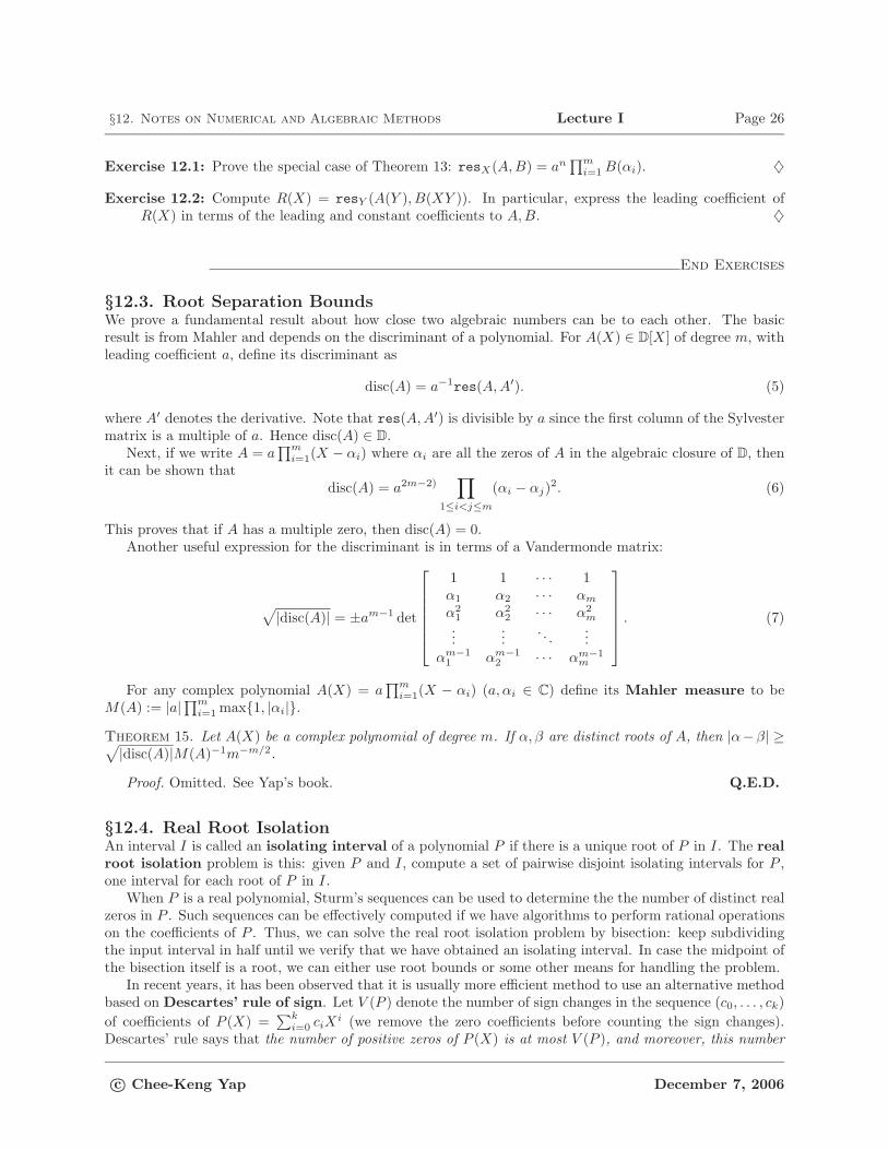
§12.3. Root Separation BoundsWe prove a fundamental result about how close two algebraic numbers can be to each other. The basicresult is from Mahler and depends on the discriminant of a polynomial. For A(X) ∈ D[X] of degree m, withleading coefficient a, define its discriminant as

disc(A) = a−1res(A,A′). (5)

where A′ denotes the derivative. Note that res(A,A′) is divisible by a since the first column of the Sylvestermatrix is a multiple of a. Hence disc(A) ∈ D.

Next, if we write A = a∏m

i=1(X − αi) where αi are all the zeros of A in the algebraic closure of D, thenit can be shown that

disc(A) = a2m−2)∏

1≤i<j≤m

(αi − αj)2. (6)

This proves that if A has a multiple zero, then disc(A) = 0.Another useful expression for the discriminant is in terms of a Vandermonde matrix:

√|disc(A)| = ±am−1 det

1 1 · · · 1α1 α2 · · · αm

α21 α2

2 · · · α2m

......

. . ....

αm−11 αm−1

2 · · · αm−1m

. (7)

For any complex polynomial A(X) = a∏m

i=1(X − αi) (a, αi ∈ C) define its Mahler measure to beM(A) := |a|∏m

i=1 max{1, |αi|}.

Theorem 15. Let A(X) be a complex polynomial of degree m. If α, β are distinct roots of A, then |α−β| ≥√|disc(A)|M(A)−1m−m/2.

Proof. Omitted. See Yap’s book. Q.E.D.

§12.4. Real Root IsolationAn interval I is called an isolating interval of a polynomial P if there is a unique root of P in I. The realroot isolation problem is this: given P and I, compute a set of pairwise disjoint isolating intervals for P ,one interval for each root of P in I.

When P is a real polynomial, Sturm’s sequences can be used to determine the the number of distinct realzeros in P . Such sequences can be effectively computed if we have algorithms to perform rational operationson the coefficients of P . Thus, we can solve the real root isolation problem by bisection: keep subdividingthe input interval in half until we verify that we have obtained an isolating interval. In case the midpoint ofthe bisection itself is a root, we can either use root bounds or some other means for handling the problem.

In recent years, it has been observed that it is usually more efficient method to use an alternative methodbased on Descartes’ rule of sign. Let V (P ) denote the number of sign changes in the sequence (c0, . . . , ck)

of coefficients of P (X) =∑k

i=0 ciXi (we remove the zero coefficients before counting the sign changes).

Descartes’ rule says that the number of positive zeros of P (X) is at most V (P ), and moreover, this number



is less than V (P ) be an even number. In particular, if V (P ) = 0 or V (P ) = 1, the rule gives us the correctnumber of positive zeros of P . For instance, if P (X) = X21 − 4X15 −X8 + 5X3 − 1 then V (P ) = 3; andhence P has at most 3 positive roots.

Suppose degP = k, and let K = [ac ,

bd ] be an interval where a, b, c, d ∈ R, c, d > 0. Consider the linear

fractional transformation (also called Mobius transformation) MK(X) = bX+adX+c . If we allow arbitrary

real values for a, b, c, d, then we can choose c = d = 1, and thus have MK(X) = bX+aX+1 . But in general, we

like a, b, c, d to be integers. Further, it is best if c, d are powers of 2 (reflecting the fact that the endpoints ofK are bigfloats). Clearly, MK maps reals to reals. But more can be said:

MK(0) =a

c, MK(∞) =

b

d.

Moreover, for 0 < s < t <∞, we have

a

c< MK(s) < MK(t) <

b

d.

In other words, M maps the interval [a/c, b/d] continuously into [0,∞].For any real polynomial P (X) and any Mobius transformation M , define the transformed polynomial

PM (X) := (cX + d)kP (M(X)).

We may also write PK(X) for PM (X) if M = MK . Then we see that α ∈ C is a zero of P (X) iff M−1(α) isa zero of PM (X). In particular, the zeros α of P in K are mapped bijectively into the zeros M−1(α) of PM

in [0,∞]. Thus, Descartes’ rule of sign can be applied to PM (X) to estimate the number of roots of P in K.In order for this to yield an algorithm for bisection, we need to be assured that when K is small enough,

V ar(PK) would be 0 or 1. This is true provided P is square-free. The relevant lemma is called the 1-circleand 2-circle lemmas:

Lemma 16 (One Circle). Let P ∈ R[X] and K = [a, b] ⊆ R. If DK is the disc with diameter K contains nozero of P (X), then V (PK) = 0.

Proof. Let M be the Mobius transformation MK . We check that M−1 maps DK to the half-space to theright of the imaginary (vertical) axis of the complex plane. Hence PK have factors of the form X + α orX2 + 2α+ β where α, β are real positive numbers. Clearly, a product of such factors has no sign variation.

Q.E.D.

Lemma 17 (Two Circle). Let P ∈ R[X] and K = [a, b] ⊆ R. Let TK and TK be the equilateral triangles,each with K as one of its side. If DK ,DK are the two discs whose boundary circumscribe these triangles. IfDK ∪DK contain exactly one real zero of P (X) then V (PK) = 1.

Proof sketch: our proof depends on Ostrowski’s theory of normal polynomials: if ai are the coefficientsof a normal polynomial Q(X) =

∑i aiX

i, then a2i > ai−1ai+1 for each i. Thus ai

ai+1> ai−1

aifor all i. We

note that M−1K maps DK ∪DK to a cone region (see Figure). Moreover, if Q(X) is normal, then it is easily

seen that V (Q(X)(X − α)) = 1 where α > 0: That is because

Q(X)(X − α) =∑

i

(ai+1 − αai)Xi

=∑

i

ai(ai−1

ai− α)Xi

=∑

i

aibiXi.

And we can see that the sequence of bi’s change sign exactly once. This shows that V (Q) = 1.

Exercises



Exercise 12.3: Implement in Core Library Descartes’ algorithm to search for real zeros in an interval [a, b].♦

End Exercises

§12.5. Bernstein Polynomials

Bernstein polynomials gives us a different view of the Descartes’ method. Moreover, it has some importantadvantages, and is useful when generalized to higher dimensions.

Let n ≥ 1 and i = 0, . . . , n. Also let a < b be real numbers. A Bernstein basis is

Bni (X; a, b) =

(n

i

)(X − a)i(b−X)n−i

(b− a)n.

When (a, b) = (0, 1), then we simply write Bni (X). It is well known that every polynomial P (X) of degree

n can be written as

P (X) =

n∑

i=0

ciBni (X; a, b)

where ci ∈ R are called the Bernstein coefficients of P (X).

§12.6. Isolating Interval RepresentationWe can use isolating intervals to represent real algebraic numbers. The isolating interval representationof a real algebraic number α is a pair (A(X), I) such that A(α) = 0, A(X) is a square-free integer polynomial,and I is an isolating interval of A containing α. We write α ≃ (A, I) in this case. We now discuss arithmeticoperations on such representations.

Note that in this representation, we could easily determine if a given (A, I) represents α = 0.Given α ≃ (A, I) and β ≃ (B, J), we want to compute α+β. First compute C = resY (A(Y ), B(X−Y )).

By Theorem 14(i), we know that α+β is a root of C. First, we replace C by its square-free part, C/GCD(C,C ′)where C ′ is dC/dX. Next, we compute K = I + J (using interval arithmetic) and check whether the signvariation V (CK(X)) is equal to 1. If so, (C,K) is our desired representation of α+β. If not, we successivelyrefine I and J , and repeat this test. We will eventually succeed, for the same reason that our root isolationalgorithm halts.

Similarly, using the other resultants described in Theorem 14, we can subtract, multiply and divide suchrepresentations.

We also need to determine the sign of a given α ≃ (A, I) But this is easy if 0 6∈ I. Otherwise, if I = [a, b],we just check whether [a, 0] or [0, b] is an isolating interval of A. This means that we can compare two realalgebraic numbers α, β by determining the sign of α− β.

Exercises

Exercise 12.4: (a) Implement in Core Library the indicated algorithms for performing the four arithmeticoperations.(b) Implement comparison of real algebraic numbers.(c) Implement square-root. ♦

Exercise 12.5: Suppose A(X) is a polynomial whose coefficients are real algebraic numbers represented byisolating intervals. How can you isolate all the zeros of A(X). ♦

End Exercises



§12.7. Subresultants

Let S0 be the Sylvester matrix for A,B ∈ D[X] of degrees m and n (m ≥ n ≥ 1). For i = 0, . . . , n,we now define the matrix Si obtained by deleting the last i rows of coefficients of A, and the last i rows ofcoefficients of B, and the last i columns of the result. Thus Si has shape (m+n−2i)× (m+n− i). Further,let S′

i denote the square matrix obtained by deleting the last i columns of Si. We call det(Si) the principalsubresultant coefficient of A,B, denoted psci(A,B). Then, psc0(A,B) is just the resultant of A,B.

Theorem 12 can be generalized:

Theorem 18. deg(GCD(A,B)) ≥ k iff psci(A,B) = 0 for i = 0, . . . , k.

Proof. The base case is Theorem 12. Use induction on k. Q.E.D.

§12.8. Homogeneous Polynomials

Now assume A,B ∈ D′[X1] where D′ = D[X2, . . . ,Xr], r ≥ 1, and D is a UFD. Thus A,B ∈ D[X1, . . . ,Xr]are multivariate polynomials. Let resX1

(A,B) ∈ D[X2, . . . ,Xr] denote the resultant where A,B are viewedas polynomials in X1. To avoid double subscripts, we write res1(A,B) instead of resX1

(A,B).More generally, define resi(A,B) (for i = 1, . . . , r) as the resultant with respect to Xi. Alternatively, the

subscript i or Xi says we are “eliminating Xi” from the system of equations A = B = 0. In examples, weusually write X for X1, Y for X2 and Z for X3. Now, when we speak of the “degree” of A ∈ D[X1, . . . ,Xr],we mean its total degree in X1, . . . ,Xr, still denoted deg(A). Also, let degi(A) denote the degree of Aas a polynomial in Xi. For example, if A = X3Y − XY + 2 then deg(A) = 4, deg1(A) = 3,deg2(Y ) = 1(assuming X = X1 and Y = X2).

A multivariate polynomial can be written as

A =∑

e∈I

ceXe, ce ∈ D

where I ⊆ Nr is a finite set and Xe = Xe1

1 · · ·Xerr where e = (e1, . . . , er). If ce 6= 0, then we say Xe occurs

in A and call ceXe a term of A. The polynomial A is Xi-regular if X

deg(A)i occurs in A. We simply say

“regular” for X1-regular.Let |e| = e1 + · · · + er. So deg(A) = maxe∈I |e|. We say A is homogeneous if |e| = |f | for all e, f ∈ I.

The zero polynomial is, by definition, homogeneous and has degree −∞.The following property can be used as the definition of homogeneous polynomials: let A ∈ D[X1, . . . ,Xr]

have degree m. Then A is homogeneous iff for all nonzero t ∈ D,

A(tX1, . . . , tXr) = tmA(X1, . . . ,Xr). (8)

Another property is Euler’s identity:

mA(X1, . . . ,Xr) =

r∑

i=1

Xi∂A

∂Xi. (9)

If A ∈ D[X1, . . . ,Xr], let A ∈ D[X1, . . . ,Xr,W ] denote the standard homogenization of A using a new

variable W , with the property that deg(A) = deg(A) and A(X1, . . . ,Xr, 1) = A(X1, . . . ,Xr). Also, for

B ∈ D[X1, . . . ,Xr,W ], let B∨ denote the operation of substituting W = 1 in B. Thus, A∨ = A.

Lemma 19. If A,B be arbitrary polynomials (not necessarily homogeneous).

(i) AB = AB

(ii) A+B = A+ BXdeg(A)−deg(B)0 (where deg(A) ≥ deg(B))

(iii) GCD(A, B) = GCD(A,B).



We are ready to prove the main result of this section.

Theorem 20. Let A,B be regular homogeneous polynomials in r ≥ 2 variables, of degrees m and n respec-tively. If res1(A,B) 6= 0 then res1(A,B) is homogeneous of degree mn.

Proof. Write A =∑m

i=0 aiXi and B =

∑nj=0 biX

i where X = X1 and ai, bj ∈ D[V ] where, for simplicity,we write V for (X2, . . . ,Xr). By homogeneity, either ai = 0 or deg(ai) = m−i for all i = 0, . . . ,m. Similarly,either bj = 0 or deg(bj) = n−j for j = 0, . . . , n. Let R(V ) = res1(A,B). For any t, let tV = (tX2, . . . , tXr).From (8), we conclude that

R(tV ) =

am tam−1 · · · tma0


. . .. . .


bn tbn−1 · · · tn−1b1 tnb0bn tbn−1 · · · tn−1b1 tnb0

. . .. . .

bn tbn−1 · · · tnb0

.

If we next multiply the ith row of A’s by ti−1 and the jth row of the B’s by tj−1, we obtain

tpR(tV )

=


tam t2am−1 · · · tm+1a0

. . .. . .

tn−1am tnam−1 · · · tm+n−1a0

bn tbn−1 · · · tn−1b1 tnb0tbn t2bn−1 · · · tnb1 tn+1b0

. . .. . .

tm−1bn tm−2bn−1 · · · tm+n−1b0

.

where p =(m2

)+

(n2

). But in the righthand side determinant, we can extract a factor of ti−1 from the ith

column (for i = 1, . . . ,m+ n). Hence the righthand side determinant is equal to

t(m+n

2 )R(V ).

This proves that

tpR(tV ) = t(m+n

2 )R(V ).

Hence R(V ) is homogeneous and its degree is

(m+ n

2

)−

(m

2

)−

(n

2

)= mn.

Instead of a direct calculation, the reader may instantly see the truth of this last equation in terms of itscombinatorial interpretation. Q.E.D.

Corollary 21. Suppose A,B ∈ D[X1, . . . ,Xr] are regular polynomials, not necessarily homogeneous. Thenres1(A,B), if non-zero, has degree ≤ mn in X2, . . . ,Xr.



Proof. First, we homogenize A and B to A and B, using a new variable X0. Our theorem says thatR(X0,X1, . . . ,Xr) = res1(A, B) is homogeneous of degreemn. Since res1(A,B) is equal toR(1,X1, . . . ,Xr),the degree of res1(A,B) is at most deg(R(X0,X1, . . . ,Xr)) = mn. Q.E.D.

Suppose the polynomial A =∑m

i=0 aiXi (ai ∈ D[X2, . . . ,Xr]) is not regular, i.e., a0 6∈ D. What can we

do? One possibility is make divide A by a0. The coefficients of A/a0 can now be viewed as elements of ameromorphic series (i.e., power series with finitely many terms with negative powers). In essense, this isNewton’s approach. See [1, Lect. 9] for this development. A simpler approach is to consider the followingtransformation:

Xi 7→ Yi + ciX, (i = 2, . . . , r).

The polynomial A′(X,Y2, . . . , Yr) = A(X,Y2 + c2X, . . . , Yr + crX) will be regular for some choice of the ci’s.In practice, this will turn a sparse polynomial into a very dense one.

This theorem will be generalized in an exercise. The proof also shows the following result:

Lemma 22. Let A =∑m

i=0 aiXi, and B =

∑nj=0 bjX

j be polynomials where the coefficients ai, bj areindeterminates. We define deg(ai) = m−i and deg(bj) = n−j, so that A,B can be regarded as homogeneouspolynomials. Then res(A,B) is a homogeneous polynomial in D[a,b] = D[a0, . . . , am, b0, . . . , bn].

Exercises

Exercise 12.6: Given A,B ∈ D[X,Y ], consider the polynomial

∆(X,Y ) =

det

[A(X) B(X)A(Y ) B(Y )

]

X − Y .

(a) Every common root α of A and B satisfies ∆(α, Y ) = 0.(b) Conversely, if deg(A) = deg(B) and ∆(α, Y ) = 0 then α is a common zero of A,B.(c) Construct a determinant R(A,B) in the coefficients of A,B such that R = 0 iff A,B has a commonzero. The determinant R(A,B) is known as the Bezout resultant of A,B.(d) If A,B have degree 2, show that R(A,B) is the same as the usual resultant res(A,B).(e) If deg(A) = 2 and deg(B) = 3, how is R(A,B) related to res(A,B)? Generalize this observation.

♦Exercise 12.7: Given A,B,C ∈ D[X,Y,Z], consider

∆(X,Y,X, Y ) =

det

A(X,Y ) B(X,Y ) C(X,Y )A(X,Y ) B(X,Y ) C(X,Y )A(X,Y ) B(X,Y ) C(X,Y )

(X −X)(Y − Y ).

(a) Show that every common zero (α, β) of A,B,C satisfies ∆(α, β,X, Y ) = 0.(b) Conversely, if degi(A) = degi(B) = degi(C) (i = X,Y ) and ∆(α, β,X, Y ) = 0. then (α, β) is acommon zero of A,B,C.(c) Construct a determinant R(A,B,C) in the coefficients of A,B,C such that the vanishing ofR(A,B,C) is equivalent to R(A,B,C) having a common zero. This is known as the Dixon resul-tant of A,B,C. ♦

Exercise 12.8: Let A,B ∈ D[X1, . . . ,Xr] be homogeneous with deg(A) = m,deg(B) = n. If degi(A)denotes the degree of A in Xi, let deg1(A) = m′,deg1(B) = n′. Write µ = m −m′ and ν = n − n′.Thus A,B are regular iff µ = ν = 0. We have the following generalization of a theorem in the text: ifres1(A,B) 6= 0 then res1(A,B) is homogeneous of degree mn− µν. ♦

End Exercises



§12.9. Weak Bezout Theorem for Curves

Bezout’s theorem that that two curves of degress m and n intersect in exact mn points, when propertycounted with multiplicities in projective space over the algebraic closure of D. The weak form simply saysthat that are at most mn intersection points.

Let A(X,Y ) = 0 and B(X,Y ) = 0 be two real algebraic curves, and write R(Y ) = resX(A,B). We mayassume that A,B ∈ Z[X,Y ].

Suppose p0 = (x0, y0) ∈ R2 is an intersection point of the two curves. Consider the polynomials A0(X) =A(X, y0) and B0(X) = B(X, y0) in R[X]: they have a common zero since A0(x0) = B0(x0) = 0. Hencedeg(gcd(A0, B0)) > 0. Hence resX(A0, B0) = 0. Is resX(A0, B0) the same as R(y0)? The answer is in thenext lemma.

Write A(X,Y ) =∑m

i=0 aiXi and B(X,Y ) =

∑nj=0 bjX

j where ai, bj ∈ Z[Y ]. Write resX(A0, B0) as thedeterminant of the matrix S0 where S0 is the Sylvester matrix for A0, B0. Similarly, let resX(A,B) = det(S)for another Sylvester matrix. Write S(y0) for the matrix obtained from S by setting Y = y0. So the questionis whether S0 = S(y0). Note that S0 depends on the degrees of A0 and B0. It is now easy to see:

Lemma 23.(i) If am(y0)bn(y0) 6= 0 then R(y0) = resX(A0, B0). (ii) If am(y0) 6= 0 or bn(y0) 6= 0 then R(y0) = 0 iffresX(A0, B0) = 0.

Proof. Under the hypothesis of (i), the Sylvester matrix for resX(A0, B0) is just the specialization of theSylvester matrix for resX(A,B). Under the weaker hypothesis of (ii), the Sylvester matrix for resX(A0, B0)may just miss a few leading rows of A0 or B0. To be specific, assume am(y0) = 0 but bn(y0) 6= 0. Then wesee that

R(y0) = bn(y0)kresX(A0, B0) = 0

if the degree of A0 drops by k ≥ 1. This proves (ii). Q.E.D.

Part (ii) in this lemma is more useful to us than part (i). We can rephrase (ii) as follows. SupposeR(y0) = 0. Then provided am(y0) 6= 0 or bn(y0) 6= 0, we conclude that there exists x0 such that (x0, y0) is acommon solution of A(X,Y ) = B(X,Y ) = 0.

Elimination as Projection Operator. For S ⊆ R2, let π(S) = {y0 : (∃x0)[(x0, y0) ∈ S]} denote theX-projection operator. Thus, the algebraic operation of computing resultant which eliminates the X-variable amounts to the geometric operation of “projecting out the X-coordinate”. Let Zero(A,B) ⊆ R2

denote the zero set of A,B. This shows that

π1(Zero(A,B)) ⊆ Zero(R).

Intuitively, computing R = resX(A,B) corresponds to computing the X-projection of the zero set. Wecould also project out the Y -coordinate, and obtain the analogous result:

π2(Zero(A,B)) ⊆ Zero(resY (A,B)).

Let us give another application of the above lemma: suppose AY = ∂A/∂Y . Similarly for AX . Definethe set of singularities of A to be Sing(A) := Zero(A,AX , AY ). Note that Sing(A) includes all self-intersections of A, and isolated points of Zero(A).

π2(Sing(A)) ⊆ Zero(resY (A,AY ).

Regular Curves. The preceding discussion motivates the next defintion: a curve A(X,Y ) = 0 is said tobe regular (or X-regular) in case degX(A) = m and am is a constant. In other words,

A(X,Y ) =

m∑

i=0

ai(Y )Xi



where am(Y ) is a constant and degY (ai) ≤ m− i. It is easy to see that by a shear transformation

(X,Y ) 7→ (X,Y + cX)

for almost every constant c, the curve can be made regular (Exercise). We can now prove the weak versionof Bezout’s theorem.

Theorem 24 (Bezout). Suppose A(X,Y ), B(X,Y ) are relatively prime and deg(A) = m,deg(B) = n. Thenthe curves A = 0 and B = 0 has at most mn common points of intersection.

Proof. By a linear translation, we may assume that A and B are regular. Let R(Y ) = resX(A,B). Sincethey are relatively prime, R(Y ) is non-zero. Hence deg(R) ≤ mn. If (xi, yi) (i = 0, 1, . . . ,mn) are mn + 1distinct common intersections, then by a rotation of the curves, we further assume the yi’s are distinct. Itfollows that R(yi) = 0 for each i. This is a contradiction since there the degree of R(Y ) ≤ mn. Q.E.D.

Remark: Bezout’s theorem generalize to arbitrary dimensions: given a system of n real polynomials invariables X1, . . . ,Xn, if these polynomials have degrees m1, . . . ,mn, then there are at most

∏ni=1mi non-

degenerate zeros. A zero x = (x1, . . . , xn) of the system is degenerate if the Jacobian vanishes at x. Thistheorem can be further generalized to polynomials in X1, . . . ,Xn and also in exponential terms of the formin eX1 , . . . , eXn (Hovanskii’s Theorem).

§12.10. Interval Arithmetic

To speed up algebraic computation, we would like to reduce algebraic computation to numerical com-putation. Numerical computation has the connotation of approximation and uncertainty. So to preservethe exactness that is normally associated with algebraic computation, we must to use some form of intervalarithmetic in our numerical computation. The basic idea of interval arithmetic is that we replace a realnumber x by an interval [a, b] that contains x. We interprete [a, b] as the “interval of uncertainty” associ-ated with x. It is easy enough to extend the basic arithmetic operations (±,×,÷) to such intervals. Fromsuch simple ideas, we encounter a rich area of research associated with extending this to more complicatednumerical computations. Interval arithmetic is an active area of research that has been greatly influencedby the work of R.E. Moore. More generally, looking beyond arithmetic, it is called validated computing.

Boxes and Interval Vectors. Let (Rn) denote the set of closed axes-parallel n-dimensional rectangleswhich we call n-boxes (or simply, boxes). In particular, for n = 1, R is the set of closed real intervals, [a, b]where a ≤ b and a, b ∈ R. A typical element of Rn has the form B = I1 × · · · × In where I1, . . . , In ∈ R.Note that a box B is to be distinguished from the corresponding interval vector (I1, . . . , In). Below, wewill need interval vectors when we discuss the interval analogue of the gradient of a function f : Rn → R.Let ( R)n denote the set of interval n-vectors. We will simply write “ Rn” for both (Rn) and ( R)n, sincethe context will make clear which is intended.

Each box B is regarded as a subset of Rn. We shall regard R as a subset of R where a ∈ R is identifiedwith [a, b] ∈ R. Similarly, Rn ⊆ Rn for all n ≥ 1.

For an interval x, let x and x denote its lower and upper bounds, i.e., x = [x, x]. Let width(x) := x−xdenote the width of an interval x. Also, mid(x) = x−x

2 denote the midpoint of x. We extend these conceptsto boxes: width(x1 × · · · × xn) := maxn

i=1 width(xi), and mid(x1 × · · · × xn) := (mid(x1), . . . ,mid(xn)).

Interval Arithmetic. Arithmetic (+,−,×,÷) on real numbers can be extended to intervals in the obviousway. E.g., x ± y = [x ± y, x ± y]. For multiplication, we need to consider all four combinations of the endpoints, xy = [min{xy, xy, xy, xy},max{xy, xy, xy, xy}]. Similarly for division x/y provided 0 6∈ y.

Comparison of intervals is only defined for certain pairs: we say I ≤ J if for all x ∈ I, y ∈ J , we havex ≤ y. Equivalently, I ≤ J . Similarly, I < J if for all x ∈ I, y ∈ J , we have x < y. Equivalently, I < J .E.g., we may write I > 0 for a positive interval.


§13. Algebraic Cell Decomposition Lecture I Page 34

For any function f : Rn → R, let f : Rn → R denote some box-valued version of f , with the property

f(B) ⊆ f(B)

and satisfying the convergence property: if Bi+1 ⊆ Bi for all i ≥ 1 and limi→∞ width(Bi) → 0, thenwidth( f(Bi))→ 0. Now, if f is a continuous function then Bi → p implies f(Bi)→ f(p).

If f is a polynomial, then f is easy to implement using interval arithmetic: we just take any methodto evaluate f , but now assume the interval analogues of the evaluation. E.g., if f(x) = 2x2 − 3x, wecan evaluate f as the sum of two monomials, 2x2 and −3x. Let x = [−1, 2]. Then x2 = [−2, 4] andf(x) = [−4, 8]+[−6, 3] = [−10, 11]. Next consider evaluating f(x) using Horner’s rule, f(x) = (2x−3)x =

([−2, 4]− 3)[−1, 2] = [−5, 1][−1, 2] = [−10, 5].This example shows that interval evaluations depends on the order of evaluation. For every polynomial,

there are two obvious methods of evaluation, as illustrated above: (1) the power method (compute all powersof x first, form all the monomials, and finally add the monomials) and (2) Horner’s rule. It is not hard toshow that (2) gives an interval that is no larger than (1). This result follows from the subdistributivity lawfor interval arithmetic:

I(J +K) ⊆ IJ + IK.

More generally, for any algebraic expression F (x) that evaluates to f(x), there is an associated intervalfunction F that represents f(x). Note that we view expressions as DAGs or equivalently, straightlineprograms. The investigation of optimal methods for constructing box functions, not necessarily derived fromevaluation of expressions, is studied in interval arithmetic (see Ratschek and Rokne [6]).

Suppose f is a multivariate polynomial in x1, . . . , xn. We want to generalize Horner’s rule for evaluatingf at the box B = I1 × · · · × In. We can view f(x) as a polynomial in xn, whose coefficients are polynomialsin x1, . . . , xn−1. Then recursively, we evaluate the coefficients of f at the box I1 × · · · × In−1. Finally, weuse the univariate version of f to evaluate it at In. By reordering the variables, we get different algorithms.It is by no means clear which ordering gives the best results.

How to confirm the shape of a curve inside a box (up to isotopy)? Consider a curve f(X,Y ) = 0which is non-singular. Consider a box B ∈ R2 whose corners are v0, v1, v2, v3 (in clockwise order, with thenorthwest corner at v0). Suppose f(v0)f(v1) < 0. Thus the curve passes through B. Let fX , fY denotethe partial derivatives of f with respect to X and Y . Thus the gradient of f is ∇f = (fX , fY ). SupposefX(C) > 0.

Exercises

Exercise 12.9: Prove that if B ⊆ R2 is a square box and for all p, q ∈ B, we have 〈∇f(p),∇f(q)〉 > 0 thenf = 0 is parametrizable in the x- or y-direction. ♦

Exercise 12.10: What other shapes besides a square box would permit such a conclusion? ♦

Exercise 12.11: Generalize the above argument to multidimensional cubes. ♦

End Exercises

§13. Algebraic Cell Decomposition

The problem before us is a very general one: given a set of polynomials P ⊆ Z[X1, . . . ,Xn], and a openregion R ⊆ Rn, to compute a partition K of R into cells such that over each cell, P is sign-invariant. Bya cell (or d-cell) we mean a subset of Rn that is homeomorphic to some open ball Bd (d = 1, . . . , n) or asingleton (d = 0). Typically, R is the interior of a box in Rn, and we call R the region of interest (ROI).

We say P is sign-invariant over a cell β ∈ K if there is a sign assignment σ : P → {+, 0,−} suchthat for all b ⊆ β and f ∈ P , f(b) has the sign σ(f). An example will clarify this concept: in Figure 10, we


§13. Algebraic Cell Decomposition Lecture I Page 35

see a partition K of the region R into cells of dimensions 0, 1 and 2. The set P = {f, g} corresponds to twocurves where f has a loop and g is an ellipse. Assume f is positive inside the loop, and g is positive insidethe ellipse. Note that K has six 2-cells, seven 1-cells and two 0-cells in K. The sign assignments for each ofthe 2-cells are indicated. The sign assignments for the 1- and 0-cells are also easily deduced.

g = 0

f = 0

(+,−)

(+,−)

(+, +)

(−, +)(−,−)(−,−)

R

Figure 10: Cell Decomposition

Depending on the applications, we may need additional properties of the cell decomposition K:

• We may want K to be cylindrical (see below) for purposes of quantifier elimination.

• We may want to compute adjacency information in applications such as motion planning. Two cellsβ, β′ are adjacent if β ∪ β′ is connected. If β, β′ are adjacent and dim(β) = dim(β′) + 1, then wesay β′ is incident on β. Note that incidence is an asymmetric relation, unlike adjacency. We maynow define the incidence graph of K to be the directed graph whose vertices are the cells of K andβ′ → β is an edge iff β′ is incident on β.

• We may need to determine a point p in each cell β ∈ K, where p is called a sample point. If β hasdimension k ≥ 0, we can ensure that k of the coordinates of p are rational numbers.

• We may want K to form a regular cell complex for the purposes of computing certain topologicalinvariants of the underlying space.

The basic tool for constructing cell decompositions K is the projection operator. Suppose S ∈ Rn andi = 1, . . . , n. Then Πi(S) = {(x1, . . . , xi, . . . , xn) : (x1, . . . , xn) ∈ S} denotes the i-th projection operator.Also, let πi(S) = {xi : (x1, . . . , xn) ∈ S}.

Suppose S = Zero(A(X,Y ), B(X,Y )) and R(X) = resY (A,B). Also let am(X), bn(X) be the leadingcoefficients of A,B. For all x ∈ R, R(x) = 0 implies(i) am(x) = 0 and bn(x) = 0, or(ii) there exists a y such that A(x, y) = B(x, y) = 0.Thus

Π2(Zero(A,B)) ⊆ Zero(R).

We may therefore think of R(X) = resY (A,B) as the algebraic analogue of projection along the Y -axis.Overview: suppose P ⊆ Z[X1, . . . ,Xn] and K is a cell decomposition of some open box R ⊆ Rn. We say

K is a P -invariant cell decomposition if P is sign-invariant over each cell of K. Let Πn(K) denote theset {Πn(S) : S ∈ K}. A cell decomposition K is cylindrical for R ⊆ R if K is a partition of R and:

• If n = 1 then this simply means that Zero(f)∩R ⊆ K for each f ∈ P . So assume n > 1 in the rest ofthis.

• Πn(K) is cell decomposition of Πn(R).


§14. Meshing Lecture I Page 36

• For each cell β′ ∈ Πn(K), consider the set of cells β ∈ K such that Πn(β) = β′. This set is called thestack over β′, denoted stack(β′).

• There is a total ordering on the elements in stack(β′) such if β1 < β2 < · · ·βm is the ordering, and ifpi ∈ βi (for each i) then the n-th component of pi’s would be sorted in the same order.

• If dim(β′) = d then dim(βi) is either d or d+1. We call β a section if its dimension is d, and a sectorif its dimension is d+ 1.

When n = 1, the cell decomposition of P is easy: it is just real root isolation. For n > 1, our goalis to define a set P ′ = Proj(P ) ⊆ Z[X1, . . . ,Xn−1] such that if K ′ is a P ′-invariant cell decompositionof Projn(R) then we can obtain a P -invariant cell decomposition K such that K ′ = Πn(K). We defineProj(P ) as the set comprising the following polynomials: let f, g ∈ P and f 6= g.

• Write f =∑m

i=0 fiXim where fi ∈ Z[X1, . . . ,Xn−1]. Then for each k = 0, . . . ,m, we add fk to Proj(P )

whenever fk is non-constant.

• Add the discriminant psck(f, f ′) to Proj(P ) for each k = 0, . . . ,degn(f)− 2 where f ′ = ∂f/∂Xn.

• Add psck(f, g) to Proj(P ) for each k = 0, . . . ,min(degn f,degn g)

The problem could be reduced to single polynomial p =∏P , obtained as a product of all the polynomials

in P . In practice, this can be quite inefficient.We claim that we can “lift” (opposite of project) K ′ to K as follows: consider the cylinder β′ ×R ⊆ Rn

where β′ ∈ K ′. For each b ∈ β′ and f ∈ P , we do the real root isolation of f(b,Xn). The number of thesereal roots do not depend on the choice of b. Let fi(b) denote the i-th root function defined in this way.Moreover, if f, g ∈ P , then these root function fi(b), gj(b) are totally ordered in a way that does not dependon b: either fi(b) < gj(b) or fi(b) = gj(b) or fi(b) < gj(b). In this way, we can define the sectors and sectionsin the stack.

REMARK: this simple projection does guarantee other nice properties we might like. E.g., K need notbe a regular cell complex.

Exercises

Exercise 13.1: Using Core Library, implement a simple cell-decomposition algorithm in 2-D. To keep theproblem simple, suppose you are given three polynomial f, g, h ∈ Z[X,Y ] and an open rectangularregion R = (a, b)× (c, d), we want to compute a sign-invariant decomposition K of P = {f, g, h}. Theoutput is supposed to be the incidence graph of K. Moreover, we want some to be able to display thecurves (so we can verify your decomposition).

REMARK: you may use the tools already implemented in Core. Under ${CORE}/progs/curves/, youwill see that we have the ability to roughly trace implicit curves. You should also be able to displaythe curves (try ”make show” in this directory). ♦

Exercise 13.2: Instead of an open rectangular region R, assume that R is defined by a set of polynomialinequalities. Modify the ACD algorithm to deal with this situation. ♦

End Exercises

§14. Meshing



The Problem. The surface meshing problem is the following: given an surface S ⊆ R3 defined bythe equation F (X,Y,Z) = 0, to construct a complex K that is topologically similar to S, and which isgeometrically close to S, to within a given ε > 0. Typically, F (X,Y,Z) ∈ Z[X,Y,Z].

We may also call K a (surface) mesh. In case K is a simplicial complex, it is also called a triangulation.Although our main interest is in surface meshing, we sometimes discuss the case of curves S ⊆ R3. Meshing acurve S amounts to finding a polygonal approximation of S. There is also the problem of volume meshingto construct a 3-dimensional complex of the volume bounded by (or exterior to) some given bounded surface.

In practice, we might also be given a given rectangular region R ⊆ R3 and we only want to mesh thesubset S ∩ R. R is called the region of interest (ROI), typically R ⊆ R3. Furthermore, we can divide thedual requirements of meshing (topological and geometric) into two subproblems: the topological meshingproblem is to compute a mesh (from scratch) satisfying the topological requirement only. The meshingrefinement problem is to refine a given topologically correct mesh to satisfy the geometric requirement.Typically, the topological meshing problem is the harder of the two, and we shall focus on this.

There is a precedent for this separation of the topological and geometric requirements: if meshing thesurface f(x, y, z) = 0 is 2-D meshing, and computing polygonal approximation to a curve f(x, y) = 0 is 1-Dmeshing, then finding roots of a function f(x) may be viewed as 0-D meshing. In finding roots of f(x), wetypically subdivide the problem into the root isolation problem and the root refinement problem. These areprecisely the topological meshing and mesh refinement subproblems of 0-D meshing.

As noted by Boissonnat et al, the strongest notion of “topologically similar” has evolved in over the lastfew years. Originally, researchers just require |K| to be homeomorphic to S. Clearly, this is inadequate: if Sis a knotted torus embedded in space, we do not regard a standard unknotted torus to be a correct output.In other words, we are also interested in how S is embedded in R3.

FIGUREWe shall interpret S, |K| to be topologically similar to mean that S and |K| are ambient isotopic to each

other. Two surfaces S, S′ ⊆ R3 are ambient isotopic if there exists a continuous map

γ : [0, 1]× R3 → R3

such that:(i) For each t ∈ [0, 1], the map γt : R3 → R3 given by γt(p) = γ(t, p) is a homeomorphism;(ii) γ0(p) = p for all p ∈ R3; and(iii) γ1(S) = S′.

Such a map γ is also called an ambient isotopy from S to S′. It is an ε-ambient isotopy if, inaddition, we have ‖γ0(p)− γ1(p)‖ ≤ ε for all p ∈ S. Thus, we want |K| to be ε-ambient isotopic to S in themeshing problem.

If we restrict γ to the domain [0, 1]×S, then we obtain an isotopy. We say S is isotopic to S′ in case thereexists such an isotopy. Clearly ambient isotopy implies isotopy, which in turn implies homeomorphism. Thusthe difference between ambient isotopy and isotopy is that the former requires a simultaneous transformationof the complementary space R3 \S. But Hirsch [Differential Topology, Springer 1976] shows that, conversely,a isotopy can be extended to an ambient isotopy in the present setting.

§14.1. Generic Subdivision Algorithm

There are few current algorithms that guarantee topological correctness in the above sense. We shallstudy two such algorithms: Snyder’s algorithm and the Plantinga/Vegter algorithm. Both are based oninterval arithmetic and the paradigm of space subdivistion.

A simple example of space subdivision algorithm is the marching cube algorithm. Suppose we want tocompute a simplicial complex for the surface S : F = 0 within the rectangular region R. We subdivide R intosmaller boxes, using an octtree data structure where each rectangle is subdivided into 8 equal size sub-boxes.For each vertex v of the boxes, we evaluate the function F . If (v, v′) is an edge of a box B, and F (v)F (v′) < 0,then we know that S intersects the box (in fact, intersects an odd number of times). Therefore, this model



requires the ability to evaluate the sign of F at given points. Of course if F (v)F (v′) > 0, we are not sure ifthere is any intersection inside this box. But assuming that S does not have “features smaller than than ε”,we might be able to conclude that S does not intersect the box. In this way, we can choose the midpoint of(v, v′) as a vertex of our mesh K. We then need to know how to connect the vertices of K to form edges, andhow to form triangular faces from these edges. These decisions can be done in each box B. As the box has 8vertices, there are 28 possibilities, but by symmetry, we reduce the number of cases to 15 distinct cases. Thisis the basis of the marching cube algorithm for meshing. The problem with the Marching cube approach isthe ambiguity of constructing the triagular faces in a cube B. In fact, the problem already shows up in thecase where S is a curve and B is a square: assume that that vertices of B has the alternating sign pattern:

[FIGURE: Alternating signs]Even assuming that we know that the curve S intersect each side of the square B at most once, and S

has at most one singular point inside B, we are left with three possibilities as shown in Figure ??(b,c,d).The marching cube algorithm and the ones that follow are instances of the following abstract algorithm:

Generic Subdivision Algorithm:

Input: Region of interest R and other data.Output: A set of boxes with associated data.⊲ INITIALIZE

Let Q be a queue, initially containing just R⊲ MAIN LOOP

while Q is non-emptyRemove B from QCASE Test(B)

TRUE: Output(B)Break

FALSE: Discard (B)Break

UNDECIDED: Subdivide B into sub-boxes Bi (i = 1, . . . , k)and put each Bi into Q

END CASE⊲ POST-PROCESSING

Go through the list of outputted boxes andto produce the required output data.

For instance, Test(B) may simply check whether (1) the surface intersects B, and (2) the diameter of Bis smaller than ε. A crude curve plotting algorithm would then place a point in the center of B as a vertexof the polygonal approximation. These vertices are simply connected to neighboring boxes in some heuristicmanner.

The fundamental question is how can we guaranteed that the correctness of this algorithm? Correctnesshere means halting as well as correctness of any output. In general, this requires two additional ingredients.

• (i) We may need additional properties about S. In the following, we shall assume S is regular, meaningthat the gradient of F (X,Y,Z) does not vanish on S

• (ii) We may need to strengthen the primitives used by our meshing algorithm. We shall assume theability to perform interval evaluation of F and its derivatives. In general, f denote the interval versionof a function f .



Parametrizability. If S ⊆ R2 is the graph of a function f : R→ R, then we say3 S is x-parametrizableover R to mean that for each x0 ∈ πx(B), there is at most one y0 such that (x0, y0) ⊆ S ∩B.

Note that when S is x-parametrizable over B, we know that S is does not contain any loops inside B andalso S has no self-intersection. In case S is an algebraic curve, we know that S ∩B is non-empty iff S ∩ ∂Bis non-empty. Thus, parametrizability leads to very nice properties for meshing.

In general, let A = {k1, . . . , kr} where 1 ≤ k1 < k2 < · · · < kr ≤ n. Recall that πA((x1, . . . , xn)) =(xk1

, . . . , xkr) and for S ⊆ Rn, we have πA(S) = {πA(p) : p ∈ S}. If S ∈ Rn and y = (y1, . . . , yr) ∈ Rr, let

S|y := {(x1, . . . , xn) ∈ S : xki= yi( for all i = 1, . . . , r}.

We say that a set S ⊆ Rn is A-parametrizable over B if there is at most one zero in B|y for eachy ∈ πA(B).

For instance, with n = 3 and A = {3}, we have JA(X,Y,Z) =

[fx fy

gx gy

]where S = Zero(f, g). If

f(X,Y,Z) = X and g(x, y, z) = y, then JA(X,Y,Z) =

[1 00 1

].

FIGURE: The unit circle X2 + Y 2 = 1 is Y -parametrizable in the region B = [12 , 1] × [−1, 1], andX-parametrizable in the region B = [−1, 1]× [ 12 , 1].

We will be interested in the general situation where S = Zero(f1, . . . , fn−r) where fi : Rn → R aredifferentiable functions. First, we need several related concepts.

Let A = {1, . . . , n} \ A. Assume the elements of A are sorted as 1 ≤ ℓ1 < · · · < ℓn−r ≤ n. Consider theJacobian JA = JA(X) which is the (n− r)× (n− r) matrix [Jij ]

n−ri,j=1 where Jij = Jij(X) := ∂fi

∂Xℓj

(X).

Interval Matrices. An interval matrixM = [Mij ]ni,j=1 is a matrix whose entries are intervals, Mij ∈ R.

Suppose m = [mij ]ni,j=1 where mij ∈ R is an “ordinary matrix”. We write m ∈ M if mij ∈ Mij for all i, j.

Sometimes, we simply view M as the set of all m such that m ∈M . We shall be interested in the predicate0 6∈ detM , i.e., for all m ∈M , det(m) 6= 0.

If B ⊆ Rn, then the box version of JA is given by JA(B) = [ Jij(B)]n−ri,j=1 and Jij(B) ∈ R is the

usual box function of Jji. Thus JA(B) is an interval matrix. The following is from Snyder [?, ?] can beseen as an interval version of the implicit function theorem:

Lemma 25. Suppose S = Zero(f1, . . . , fn−r) and B ∈ Rn. Fix A = {k1, . . . , kr} as above. If 0 6∈det JA(B) then S is A-parametrizable over B.

Let us show this for the case where n = 2 and r = 1. In this case, S is the curve f(X,Y ) = 0. WithA = {1}, we have JA = ∂f

∂y = fy. Then the above lemma simplifies to the claim that 0 6∈ fy(B) implies S

is x-parametrizable over B. In proof, suppose there are two distinct points (x0, y0) and (x0, y1) in S ∩ B.Then by Rolle’s theorem, fy(x0, c) = 0 for some c ∈ (y0, y1). This contradicts the condition 0 6∈ fy(B).

This is a kind of implicit function theorem. For a semi-algebraic version of the implicit theorem, see [2,p. 134].

Meshing Using Parametrizability First consider a curve S : f(X,Y ) = 0 that is a 1-manifold. ThusS is a collection of pairwise disjoint loops or infinite curves. Snyder (1992) shows how we can compute apolynomial approximation:

3The indexing system for discussing parametrization can be confusing – should we call this x-parametrizability or y-parametrizability? We suggest the rule that x-parametrizability should mean that x can be used as a parameter for corre-sponding implicit function h, where f(x, h(x)) = 0.



Curve Approximation Algorithm:

Input: Region of interest R ⊆ R2 and a curve S : f(x, y) = 0.Output: A topologically correct polygonal approximation.⊲ INITIALIZE

Let Q be a queue, initially containing just R⊲ MAIN LOOP

while Q is non-emptyRemove B from Qif (S is x- or y-parametrizable over B):

Assume s is x-parametrizable over BCompute S ∩ ∂B = {p1, . . . , pm} using root isolation.Refine the isolating intervals until we order their x-values: p1.x < p2.x < · · · < pm.xIf m ≤ 1, discard B.Else for each i = 1, . . . ,m,

Assume ai < pi.x < bi with the (ai, bi)’s disjointIf f((bi + ai+1)/2, y) changes sign over the interval πy(B)

we “link” pi and pi+1.else

Subdivide B into sub-boxes Bi (i = 1, . . . , 4)Put each Bi into Q

⊲ POST-PROCESSINGGo through the output boxes, and identify points on the commonedges of adjacent boxes.

Note that linking pi with pi+1 are of three kinds: one of pi, pi+1 is on a vertical edge of B, pi, pi+1 lieson opposite edges of B, and pi, pi+1 lies on the same edge of B,

Does this algorithm halt? If the curve grazes the boundary edge then some root isolation strategies maynot halt. See the chapter of Vegter for an example.

§14.2. Vegter Plantinga’s Approach

We now present another approach to isotopic meshing. Assume S : f(X,Y ) = 0 is the curve and f iscontinuously differentiable. Let fx = ∂f

∂X and fy = ∂f∂Y . Assume S is non-singular, i.e., for all p ∈ S, the

gradient does not vanish:∇f(p) = (fx(p), fy(p)) 6= (0, 0).

Now, we want the interval version of the gradient, where for any box B, we define

∇f(B) := ( fx(B), fy(B)).

We can form the scalar product of this interval gradient function,

〈 ∇f(B), ∇f(B)〉 := fx(B) · fx(B) + fy(B) · fy(B)).

The algorithm is based on two basic predicates or conditions:

• C0(B) : 0 6∈ f(B).

• C1(B) : 0 6∈ 〈 ∇f(B), ∇f(B)〉.



Consequences of Small Normal Variation Condition. Clearly, if C0(B) holds, the curve does notpass through B. The condition C1(B) tells us that something equality interesting. Intuitively, it means thatthe gradient of every point in B is roughly pointing in the same general direction. More precisely, for allp, q ∈ B we have 〈∇f(p),∇f(q)〉 > 0, i.e., the gradient vectors spans an angle less than 90◦. In view ofthis, C1(B) is also known as the small normal variation condition on B. To use this condition, we needseveral

Motivation Let us see how useful this condition is: there are two ambiguities in the Marching cubealgorithm: the first ambiguity is that the sign of f at the endpoints of an side of a box only tells us theparity (odd or even) of the intersection of the curve with the side. The epsilon heuristic is that when thebox is small enough, we assume that odd equals one intersection, even equald no intersection. The secondambiguity comes from the alternating sign pattern at the corners of a square box:

FIGURE: (a) Alternating pattern (b) (c) two ways to connect four vertices.Using the epsilon heuristic, we introduce four vertices, one in the middle of each side of the box. Now,

it is unclear how to connect these four vertices within the box in a topologically correct way (fig(b) or (c)).We next see that condition C1 saves us both ambiguities.

There are several basic arguments that can be applied in is the following 2-dimensional analogue of Rolle’stheorem for real functions:

Lemma 26. Suppose f(x, y) is C1 and p, q are points such that ∇f(p),∇f(q) are not parallel. Let u =α∇f(p) + (1− α)∇f(q) for some 0 ≤ α ≤ 1. Let pt denote the point (1− t)p+ tq. Then there exists somet ∈ [0, 1] such that either ∇f(pt) = 0 or ∇f(pt) is parallel to u.

Proof. Assume that for all t ∈ [0, 1], ∇f(pt) 6= 0. Then the unit vector dt = ∇f(pt)/‖∇f(pt)‖ is well-defined for all t ∈ [0, 1]. If dt = (0, 0) for some t, then the lemma holds trivially. Otherwise, we have d0 isparallel to ∇f(p) and d1 is parallel to ∇f(q). This means that for some t ∈ [0, 1], dt must be parallel to u.

Q.E.D.

Lemma 27. Suppose C1(B) holds at a box B.(i) The curve f = 0 is parametrizable in the X- or Y -direction in B.(ii) The sign of f at the four vertices of B cannot form an alternating pattern.

Proof. (i) The condition C1(B) means that 0 6∈ fx(B) · fx(B) + fy(B) · fy(B)), and this in turnmeans that 0 6∈ fx(B) or 0 6∈ fy(B). The latter two conditions imply parametrizability in either X- orY -direction.

(ii) Suppose the sign of f is alternating, say f(NE) > 0, f(NW ) < 0, f(SW ) > 0, f(SE) < 0. Thenthere is a point p on the north side with fx(p) < 0 and a point q on the south side with fx(q) > 0. Thus0 ∈ fx(B). Similarly, 0 ∈ fy(B). This contradicts the condition C1(B). Q.E.D.

The intuitive idea is that repeated subdivision of a box B will eventually make C0 or C1 true. This isthe basis of the following algorithm:



Isotopic Curve Approximation Algorithm:

Input: Region of interest R ⊆ R2 and a curve S : f(X,Y ) = 0.Output: A topologically correct polygonal approximation.

Initialize a quadtree T whose root is B.Subdivide each leaf B′ of T until either C0(B

′) or C1(B′) holds.

Balance(T )for each box edge of leaf of the quadtree

if the signs of F at the two endpoints are oppositethen insert a vertex at the midpoint of the edge

for each leaf of Tif the leaf contains two vertices, connect them by a segmentelse if the leaf contains four verticesthen find the 2 vertices on one side,

and connect them to the other two vertices without crossing

We first prove termination:

Lemma 28. The above algorithm terminates.

Proof. There is a minimum distance ε > 0 between the solutions of f = 0 and ∇f = 0. Thus, when a boxB has radius less than ε, either 0 6∈ f(B) or 0 6∈ ∇f(B). Then, by the convergence of interval arithmetic,C0(B) or C1(B) eventually holds. Q.E.D.

Next, let us prove isotopy of the polygonal approximation. We may ignore the case where f is zero ata corner of a box. Actually, it is not hard to see that if f is zero at a corner, we can freely choose eithernon-zero sign for the corner.

First we do not consider the adaptive grid produced by the algorithm. Instead, assume that the grid isregular, i.e., all leaf boxes have the same size.

FIGURE: semicircle

Lemma 29. Assuming the regular grid, then V-P algorithm is correct.

Proof. Note that in the case, each box has either 0 or 2 vertices. Moreover, each edge has 0 or 1 vertex.We must consider the possibility of the curve cutting the boundary of B more than once. Suppose the

input curve cuts a horizontal edge twice at p, q. Then curve must be x-parametrizable in B.This curve must not exit the semicircle with diameter [p, q]. If the curve reaches a point r outside the

semicircle, then we get contradiction of C1(B). We can repeat this argument for every pair (p, q). What ifthe ends are not paired? Q.E.D.

Going back to the adaptive, balanced quadtree, we have:

Lemma 30. There are zero, two or four vertices on the boundary of each box of the balanced quadtree.

Proof. The reason for an even number is clear: each vertex is determined by the sign of f at the verticesof B or the midpoints of edges of B. Q.E.D.

Lemma 31. The polygonal approximation for the balanced quadtree is isotopic to the polygonal approximationfor the regular grid.

Proof. Q.E.D.


§15. Notes on Cohomology Lecture I Page 43

Comparison with Snyder. one big advantage over Snyder is that we do not have to find zeros (i.e.,intersect the curve C with edges of the boxes). We just do sign evaluation of f at vertices, and intervalevaluation.

Note that because Vegter-Plantinga does not need to determine the exact topology of the curves withina cell, it may terminate faster in many situations.

The extension to 3-D is similar with more case analysis. Presumably this extensions to all dimensions.

Exercises

Exercise 14.1: Provide a convincing proof of correctness of V-P. ♦

Exercise 14.2: Extend the V-P result to all dimensions. ♦

Exercise 14.3: Extend the Vegter-Plantinga result to curves which may be singular. ♦

End Exercises

§15. Notes on Cohomology

Cohomology: in some ways this is more natural than cohomology, but it was much slower in beingdeveloped. Wikipedia has a nice history. See Munkres.

The HOM Functor: If A,G are Abelian groups, we obtain another Abelian group

Hom(A,G)

of all homomorphisms of A into G. This groups is essential for defining cohomology.Some facts about Hom(A,G). Let φ, ψ ∈ Hom(A,G). Then the group operation on Hom(A,G) is

defined via (φ + ψ)(a) = φ(a) + ψ(a) for all a ∈ A. We must show that (φ + ψ) is a homomorphismfrom A to G: for all a, b ∈ A, (φ + ψ)(a + b) = φ(a + b) + ψ(a + b) = (φ(a) + φ(b)) + (ψ(a) + ψ(b)) =(φ(a) + ψ(a)) + (φ(b) + ψ(b)) = (φ + ψ)(a) + (φ + ψ)(b). Note that the zero element Hom(A,G) is thefunction φ(a) = 0 for all a ∈ A. The inverse of φ is −φ where −φ(a) = φ(−a).

Example: Hom(Z, G) is isomorphic to G, where the isomorphism assigns to φ ∈ Hom(Z, G) the elementφ(1). More generally, if A is a free Abelian group of rank n, then Hom(A,G) is isomorphic to G⊕ · · · ⊕G︸︷︷︸

n

.

Dual Homomorphism. Any homomorphism f : A → B gives rise to a dual homomorphism f goingin the reverse direction,

Hom(B,G)ef→ Hom(A,G)

where φ : B → G is mapped to

f(φ) : Af→ B

φ→ G.

The map f is a homomorphism because

[f(φ+ ψ)](a) = (φ+ ψ)(f(a)) = φ(f(a)) + ψ(f(a)) = [f(φ)](a) + [f(ψ)](a).


§15. Notes on Cohomology Lecture I Page 44

Category. We introduce the useful language of categories. A category C consists of 3 things:(i) A class of objects X.(ii) For every ordered pair (X,Y ) of objects, a set hom(X,Y ) of morphisms f . We write f : X → Y todenote that f ∈ hom(X,Y ).(iii) For every triple of objects (X,Y,Z) a function called composition of morphisms, hom(X,Y ) ×hom(Y,Z)→ hom(X,Z).If (f, g) ∈ hom(X,Y ) × hom(Y,Z), then their composition is denoted g ◦ f . These concepts satisfies twoaxioms:

Axiom 1 (Associativity). If f ∈ hom(W,X) and g ∈ hom(X,Y ) and h ∈ hom(Y,Z) then h ◦ (g ◦ f) =(h ◦ g) ◦ f .

Axiom 2 (Identities). If X is an object, there is an element 1X ∈ hom(X,X) such that

1X ◦ f = f, g ◦ 1X = g

for all f ∈ hom(W,X) and g ∈ hom(X,Y ), for all W,Y .A (covariant) functor G from category C to category D is a function assigning each object X of C to

an object G(X) of D, and each morphism f : X → Y of C to a morphism G(f) : G(Y ) → G(X) of D.Moreover, we require G(1X) = 1G(X) for all X and G(g ◦ f) = G(f) ◦G(g).

A contravariant functor G from category C to category D is a function assigning each object X of Cto an object G(X) of D, and each morphism f : X → Y of C to a morphism G(f) : G(X) → G(Y ) of D.Moreover, we require G(1X) = 1G(X) for all X and G(g ◦ f) = G(g) ◦G(f).

EXAMPLE: Let us return to our example of Abelian groups. Let C be the category of Abelian groups,where the objects are Abelian groups, and morphisms are homomorphisms of Abelian groups. Let G befixed, and D be the category whose objects are Hom(A,G) where A is any Abelian group. Then the maps

A→ Hom(A,G), and f 7→ f

defines a contravariant functor from the category C to categor D.FACT: If f : A → B is a homomorphism and is surjective, then its dual f is injective. That is, the

exactness of

Bf→ C → 0

implies the exactness of

Hom(B,G)ef← Hom(C,G)← 0

More generally (p.247):

Theorem 32. If the sequence

Af→ B

g→ C → 0

is exact, then the dual is exact:

Hom(A,G)ef← Hom(B,G)

eg← Hom(C,G)→ 0

Moreover, if f is injective, and the first sequence splits, then f is surjective and the second sequence splits.

Simplicial Cohomology Groups. Let K be a simplicial complex. G an Abelian group. The group ofp-dimensional cochains of K, with coefficients in G, is the group

Cp(K;G) = Hom(Cp(K), G)

Thus, each cochain in Cp is a homomorphism h : Cp(K) → G where h(σ) ∈ G for each simplex σ, andwe extend this map linearly. NOTE: the notation Cp(K) (from Munkres) is the same as Cp(K,Z) (integralhomology coefficients).


§16. On Permutations Lecture I Page 45

REMARK: The basic objects of homology are subspaces of the space K that we wish to study, namelyCp (think of Cp as a subspace of K). In contrast, the basic objects of cohomology are not the subspaces Cp

but but functions Cp from the subspaces (to some group G)!The coboundary operator δ is the dual of the boundary operator ∂ : Cp+1(K)→ Cp(K). Thus,

Cp+1(K;G)δ← Cp(K;G).

NOTE: δ raises (!) the dimension from p to p+ 1. Let us see how δ works: suppose φ : Cp(K)→ G. Thenδ(φ) : Cp+1(K)→ G is defined by

[δ(φ)](σp+1) = φ(∂(σp+1))

The kernel of δ (= δp)Zp(K;G) = ker δp

is called the groups of cocycles; the image of δ is

Bp(K;G) = imδp

is called the groups of coboundaries; their quotient

Hp(K;G) = Zp(K;G)/Bp(K;G)

is called the cohomology group.

Abstract Cohomology. In this case, we begin with any cochain complex,

· · · δ→ Cp δ→ Cp+1 δ→ · · ·

which is a sequence of Abelian groups and a boundary operator δ for successive pairs of this sequence. Notethe increasing index. We only require δ ◦ δ = 0. Note that such cochain complexes are normally associatedwith some topological space X.

Then the pth cohomology group of the complex is given by

Hp = {Kernel ofδ : Cp → Cp+1}/{Image ofδ : Cp−1 → Cp}.

§16. On Permutations

Permutations is a fundamental concept in computing. It is good to develop some facility for thinkingabout and for manipulating permutations.

If {i1, . . . , im} ⊆ {0, . . . , d} are m ≥ 0 distinct elements, then the sequence [i1i2 · · · im] represents thepermutation π where π(k) = k if k 6∈ {i1, . . . , im}, and otherwise π takes i1 to i2, and i2 to i3, etc, andfinally takes im to i1. We call [i1 · · · im] a cyclic permutation or m-cycle. The special cases m = 0, 1, 2 arenoteworthy: If m = 0, we write the permutation as [], and it represents the identity permutation. Similarly,for m = 1, the permutation [i1] is also the identity permutation. For m = 2, [i1i2] is called a transposition.Clearly, [i1i2] = [i2i1]. In general, we have [i1i2 · · · im] = [i2i4 · · · imi1].

Consider how cyclic permutations interact under function composition: we write composition by juxta-position: e.g., [13][14] is the composition of the transpositions [13] and [14] (we first apply the permutation[13] followed by the permutation [14]). In this case, we may verify that [13][14] = [134] 6= [143] = [14][13].Thus composition (or juxtaposition) is not commutative. Also, [13][13] = [1] = [3] = [] (the identity).

If [i1 · · · im] and [j1, . . . , jn] are two cycles and {i1, . . . , im} ∩ {j1, . . . , jn} = ∅, we say the two cycles aredisjoint. It is clear that [i1 · · · im][j1, . . . , jn] = [j1, . . . , jn][i1 · · · im] i.e., disjoint cycles do commute. Wemay verify that in general, if [i1 · · · im] = [i1i2][i1i3] · · · [i1im]. That is:

Every m-cycle (m ≥ 2) can be written as a composition of m− 1 transpositions; if the m cycle is written asa composition of k compositions then k ≥ m− 1 and k is even. (*)


§17. Assigned Homeworks Lecture I Page 46

Given a permutation π, we construct a cycle [0π(0)π2(0) · · ·πk(0)] where k ≥ 0 is the smallest value suchthat πk+1(0) = 0. Next, starting from any i1 from {0, . . . , d} \ {0, π(0), . . . , πk(0)}, we can form anothercycle starting from i1. We can keep repeating this process until we find all the cycles of π. This proves:

Every permutation can be written as composition of disjoint cycles. (**)

For instance, [053][12][4] is a permutation of {0, . . . , 5}. Usually, we omit the 1-cycles in such a representation,and write [053][12] instead.

Combining (*) and (**), we conclude that every permutation can be written as a product of transpositions.Although the number of transpositions is not unique, the parity of this number is unique. Recall π of{0, . . . , d} into a product of compositions.

Let us now see how two transpositions in juxtaposition [ij][i′j′] can be transformed. There are three cases:(1) If the two transpositions are disjoint, we already know that [ij][i′j′] = [i′j′][ij]. (2) If they are identical,we also know that they annihilate each other: [ij][ij] = []. (3) Finally, assume the two transpositions sharesexactly one common element i. In this case, we say the two transpositions are linked by the element i. Inthis case we may assume they have the form [ij][ik] where i, j, k are distinct. In this case, we can rewrite[ij][ik] as [jk][ij]. Think of this as “moving [ij] to the right, past [ik]”. But while moving [ij] to the right,the transposition [ij] survives, but the “passed over” transposition is transformed from [ik] to [jk] (i.e., theirlink element has changed from i to j). Note that the two transpositions remain linked. Consider the newpair [jk][ji]. If we move [jk] to the right, we transform it into [ki][jk], so that k is their link. In other words,we can choose their link to be any of the three elements i, j, k. To ensure canonicalness, we always make theminimum element of i, j, k the link.

In any sequence of transpositions, we can form an undirected graph whose vertices are these transpo-sitions, and whose edges connect pairs of linked transpositions. The connected components of this graphcorrespond to the cycles of the graph. By repeated local transformations, we can assume that all thetranspositions belonging to the same connected component are in contiguous positions. Note that localtransformations do not affect these graphs (although the set of transpositions may change). Further, bylocal transformations, we may assume that ALL the transpositions of the connected component are linkedto each other via a single element. We may assume the element is the least element in the set of elements ofthat component. When this happens, we can replace the component by a single cycle. In this way, we get aset of disjoint cycles. Clearly, this cycle is unique.

Given a juxtaposition of transpositions, we may simplify it as follows: (a) Suppose there are two identicaltranspositions, · · · [ij] · · · [ij] · · · . We can move the leftmost copy [ij] to the right until it is next to anothercopy of [ij]. Then we can annihilate them. So assume there are no identical transpositions. (b) Supposethere is a triple of transpositions, · · · [ij] · · · [jk] · · · [kℓ] · · · , where i, j, k, ℓ are distince, the first two are linkedby j and the next two are linked by k. Then...

§17. Assigned Homeworks

1. Sep 12. Compute the homology groups of Sn (the n-spheres).

2. Sep 12. Give the minimum triangulation of the torus T 2. Assume “minimum” means the minimumnumber of vertices.

HINTS: Use the standard representation of T by a square rectangular region in which the oppositeedges are identified. What to look out for? You must remember that in a triangular, any two verticesdetermine at most one edge, any three vertices determine at most one face. Also, Euler’s characteristicfor a torus says that v − e+ f = 0. You will need another relation involving v, e, f .

3. Sep 19. Show that the naive SNF algorithm (see our notes) can be exponential time. Exponentialmeans that it is exponential at least one of the parameters m,n,L where the matrix is m × n and Lis the maximum bit size of the entries.



4. Sep 19. Implement the ”naive” algorithm for computing SNF. Assume that on input matrix A, yououtput (S,U, V ) where S = UAV , S is in SNF, and U, V are unimodular. Test your program with anyof the examples from Vegter/Rote.

HOW TO DO THIS HOMEWORK: you must download the Core Library (http://cs.nyu.edu/exact/).Please use Core 1.7x (not the pre-release version Core 2.0). In the Core Library, we have simpleextensions (COREX). You need to use the Linear Algebra extension to use matrices and perform basicoperations.

You must do this homework in pairs (this is called Xtreme Programming, which has many benefits).Consult me if you have questions about teams. Also see the introduction of these notes for possibleuse of CYGWIN. All the software you need can be obtained through CYGWIN.

How to submit: I suggest you include a simple Makefile (there are many examples in Core Library),and tar everything into one file to send me. For basic information about Makefiles, see my web noteshttp://cs.nyu.edu/~yap/prog/make/. I would like to type ”make” in order to compile your program,and ”make snf” to see it executing on an example. To ensure that your Makefile can be directly usedby me, I want you to put all your homework 1 files inside a subdirectory named $CORE/progs/your-name/hw1/. Similarly for homework 2, etc.

5. Oct 2. Recall the standard torus T 2 used in Morse theory. One chart for T 2 has been given byVegter/Rote: it is ϕ : U → T 2 where U = (0, 2π)× (0, 2π), and

ϕ(u, v) = (r sinu, (R− r cosu) sin v, (R− r cosu) cos v).

(a) Give other charts so as to cover the rest of T 2. How many additional charts do you need?(b) Let h be the usual height function on T 2. Compute the gradient field of h.(c) Consider another different height function f(ϕ(u, v)) = r sinu. Compute the gradient field of f .(d) Is f a Morse function?

6. Oct 2. Let F (X,Y ) ∈ Z[X,Y ] and consider the curve M : F (X,Y ) = c for some rational c ∈ Q.(a) Describe how you can detect whether M is a smooth manifold. REMARKS: this is a computationalproblem. Although we do not ask for an implementation, you must describe details at the level ofimplementing this in Core Library. We view M “geometrically”, simply as the set of real solutions ofF (X,Y )− c. Thus we may assume that F (X,Y ) is squarefree. Moreover, we shall define smoothnessto mean that F (X,Y ) = FX(X,Y ) = FY (X,Y ) = 0 has no real solution.(b) Let M be smooth from (a). For p0 ∈ Q2, define the function f : M → R where f(q) = ‖p0 − q‖(Euclidean distance). Describe how to test whether f is Morse.(c) Let f be Morse from (c). Describe how to compute the critical points of f and to determine theindex of each critical point.

7. Oct 10. Let A,B ∈ D[X1, . . . ,Xr] be homogeneous with deg(A) = m,deg(B) = n. If degi(A) denotesthe degree of A in Xi, let deg1(A) = m′,deg1(B) = n′. Write µ = m − m′ and ν = n − n′. ThusA,B are regular iff µ = ν = 0. We have the following generalization of a theorem in the text: ifres1(A,B) 6= 0 then res1(A,B) is homogeneous of degree mn− µν.

8. Oct 10. Implement the following algorithm: given an interval I = [a, b], and a polynomial A(X), touse Descartes’ rule of sign to determine an upper bound on the number of zeros of A in I. Use thisalgorithm to isolate all the zeros of A in any given interval. NOTE: efficiency is not our primaryconcern in this exercise.

9. Oct 17. Implement the Descartes method for isolating the roots of a real polynomial. The input to youralgorithm should be a square-free polynomial A(X) ∈ Z[X] and an interval I = (a, b). If I contains kroots of A, your algorithm return a list of isolating intervals (J1, . . . , Jk) for these roots.



CONSIDERATIONS: In Core Library, we have a facility for inputing polynomials. The simplest way toinput them is to use the string representation E.g., ”3 Xˆ4- 17 Xˆ2 - X +11”. Please look at examplesunder the directory $(CORE)/progs/poly/. Intervals should be a pair of big floats. For bisection, donot forget to check for the midpoint being a root.

10. Oct 24. Implement in Core Library the algorithms for performing the four arithmetic operations,and also comparison of two real algebraic numbers. REMARK: you need not implement resultants ofpolynomials, which is already available in Core. Note that you should reuse the work in the previousexercise on Descartes method for root isolation.

11. Oct 30. Consider the function f(x) =√x (with the domain of f suitably defined (either in R or in

C). This is an example of an algebraic function. In general, let us say that a partial real functionf : R→ R is algebraic if it satisfies a polynomial relation of the form

F (x, f(x)) = 0

for all x in the domain of f , and F (X,Y ) ∈ Z[X,Y ]. Note that we are deliberately trying to avoid themachinery of algebraic function theory in this definition. For instance, F (X,Y ) = X − Y 2 in the caseof f(x) =

√x. Let g(y) be another algebraic function.

(a) Prove that the function composition h(x) = (g◦f)(x) = g(f(x)) is algebraic. HINT: use resultants.(b) Suppose the domain of f(x) is an interval [a, b] and f is continuous. Call c ∈ [a, b] a regular pointof f if in a sufficiently small neighborhood N of c, the function f(x) is uniquely defined by knowing thedata f(c). More precisely, for each c′ in the neighborhood of c, there is a unique choice of y such thatF (c′, y) = 0 holds. Note that by this definition, the point c = 0 is regular for the function f(x) = x2/3.How to you detect if a given point c is regular or not?

CLARIFICATION: Michael Burr points out some bugs in this question. First of all, we mustexclude the trivial case where F (X,Y ) ∈ Z[X,Y ] is identically zero. But even so, we have a counterexample: let

f(x) =

{1 if x = ex if x 6= e

,

g(x) =

{π if x = 1x if x 6= 1

,

g ◦ f =

{π if x = ex if x 6= e

.

Both f and g are algebraic according to my definition, since

F (x, f(x)) = 0 if F (X,Y ) = (Y − 1)(Y −X),

G(y, g(y)) = 0 if G(Y,Z) = (Y − 1)(Z − Y ).

Furthermore R(X,Z) = resY (F (X,Y ), G(Y,Z)) is identically 0. This does not necessarily prove thatg ◦ f is not algebraic. Pf?

One solution to these counter examples is to declare the function f above is algebraic if it is a con-stant function f(x) = c for some algebraic number c, or there exists F (X,Y ) ∈ Z[X,Y ] such thatF (x, f(x)) = 0 holds for all x in the domain of f and, in addition, whenever F (X,Y ) is primitive.This means that for all factorizations F (X,Y ) = F1(X)F2(Y )F3(X,Y ), we must have F1 and F2 tobe constants. N.B.: It is possible to check whether a given F (X,Y ) is primitive. Then, f(x) and g(x)above are no longer algebraic (pf?).



12. Oct 30. Please refer to (updated) Chapter 12 of my EGC notes on Constructive Zero Bounds. Considerthe following expression

e =√x+√y −

√x+ y + c

√x√y.

View this as a DAG that shares common subexpressions. (a) If x, y, c are L-bit integers, what is theBFMS bound for e?(b) How good is this bound? In other words, construct asymptotic example that comes as close to thisbound as possible.

13. Nov 7. Let f, g ∈ Z[X] be polynomials of degrees ≤ m and height h. Suppose f(x) = 0 and g(x) 6= 0.(a) Give a lower bound on |g(x)| in terms of m,h. HINT: you may use BFMS or Measure bounds.(b) Let F (X,Y ) ∈ Z[X,Y ]. Give a complete procedure to test if F = 0 has any solution inside agiven box B = [a, b]× [c, d] where a, b, c, d are bigfloats. Conceptually, you must reduce everything tosomething you can actually implement using Core Library. HINT: divide into two cases, whether thecurve F = 0 intersects the boundary of B or not.

14. Nov 7. Using Core Library, implement a simple cell-decomposition algorithm in 2-D. To keep theproblem simple, suppose you are given three polynomial f, g, h ∈ Z[X,Y ] and an open rectangularregion R = (a, b) × (c, d), we want to compute a sign-invariant decomposition K of P = {f, g, h}. Inorder to allow different test inputs, we want the inputs to be read from a file. The output is supposedto be the incidence graph of K. Moreover, we want some to be able to display the curves (so we canverify your decomposition).

NOTES: you may use the tools already implemented in Core. Under ${CORE}/progs/curves/, youwill see that we have the ability to roughly trace implicit curves. You should also be able to displaythe curves (try ”make show” in this directory). You should prepare several input files, and we shouldbe able to type ”make” to compile your program, ”make one” to test your first input file, ”make two”to test the second input file, etc.

15. Nov 21. Let f : R2 → R be a polynomial function, and ∇f(B) denote the interval analogue ofthe gradient function ∇f(x, y). Plantinga-Vegter claimed that if 0 6∈ 〈 ∇f(B), ∇f(B)〉, then f isparametrizable in the X- or Y -direction.

16. Nov 28.

Vegter-Plantinga Algorithm. The correctness of this algorithm seems to leave a lot to be proved.(i) Prove that each leaf box of the quadtree has either 0, 2 or 4 vertices.(ii) Prove that the curve is isotopic to the polygonal approximation.

References

[1] S. S. Abhyankar. Algebraic Geometry for Scientists and Engineers. Americal Mathematical Society,Providence, Rhode Island, 1990.

[2] S. Basu, R. Pollack, and M.-F. Roy. Algorithms in Real Algebraic Geometry. Algorithms and Computationin Mathematics. Springer, 2003.

[3] J. Boissonnat and M. Teillaud, editors. Effective Computational Geometry of Curves and Surfaces.Number 59 in Mathematiques et Applications. Springer, 2006. To appear.

[4] C. Delfinado and H.Edelsbrunner. An incremental algorithm for Betti numbers of simplicial complexeson the 3-sphere. Computer Aided Geom. Design, 12:771–784, 1995.

[5] J. R. Munkres. Topology: A First Course. Prentice-Hall, Inc, 1975.



[6] H. Ratschek and J. Rokne. Computer methods for the range of functions. Horwood Publishing Limited,Chichester, West Sussex, UK, 1984.

[7] C. K. Yap. Fundamental Problems of Algorithmic Algebra. Oxford University Press, 2000.


Date post:	06-May-2018
Category:	Documents
Upload:	trantram
View:	219 times
Download:	1 times

Computational Topology and Geometry: Supplementary …yap/classes/modeling/06f/lect/ll1.pdf ·...

Documents