Computational Vision U. Minn. Psy 5036 Daniel Kersten Lecture 15: Geometry & surfaces: depth & shape Initialize Off[General::spell1]; SetOptions[ArrayPlot, ColorFunction → "GrayTones", DataReversed → True, Frame → False, AspectRatio → Automatic, Mesh → False, PixelConstrained →{1, 1}, ImageSize → Small]; SetOptions[DensityPlot, ColorFunction → "GrayTones", Frame → False, AspectRatio → Automatic, Mesh → False, ImageSize → Small]; Outline Last time Extrastriate cortex--overview Scenes from images, scene-based modeling of images Today Geometry, shape and depth: Representation & generative models Lambertian model Surfaces, geometry & depth Introduction Recall two major tasks of vision: "Knowing what is where just by looking"--Marr's definition of vision. We introduce the problem of extracting geometrical information about the world. General issues: Between-object, viewer-object, within-object geometry. Coarse vs. dense estimations of geometrical relations.
Scenes from images, scene-based modeling of images
Today
Geometry, shape and depth: Representation & generative models
Lambertian model
Surfaces, geometry & depth
Introduction
Recall two major tasks of vision: "Knowing what is where just by looking"--Marr's definition of vision. We introduce the problem of extracting geometrical information about the world.
General issues: Between-object, viewer-object, within-object geometry.Coarse vs. dense estimations of geometrical relations.
The projection constraint
The fundamental geometrical constraint in vision is that 3D points in the world are projected onto 2D surfaces--one on each retina.
The figure below illustrates the geometry. We make the simplification of assuming a pin hole model of the eye where we don’t have to worry about optical aberrations. We also use the simplifying conven-tion of representing the image in the conjugate plane to the retina. Let the retina, i.e. the image plane, be perpendicular to the Z-axis, and positioned at Z=-f units behind the pin hole. The pin hole is the origin of our 3D world coordinate system, (X,Y,Z). Imagine that the retina is the “object” that is being imaged as a surface--the retinal plane’s conjugate plane--intersecting the positive Z-axis (blue rectan-gle below). The conjugate plane corresponds to the image of the retina outside of the eye positioned at Z = +f units. Simplifying further, with f=1, the coordinates of points in the conjugate plane, (x,y) can be mapped onto retinal coordinates (x’,y’) by (-x,-y).
More generally, for a “thin” lens approximation, the origin represents the nodal point of the eye--where light rays pass through undeviated. For a more realistic, “thick” lens, there are two nodal points.
Let {X’,Y’,Z’} represent the coordinates of a specific point in the world. {X’,Y’,Z’} projects to {x,y} in the conjugate image plane.
If we let the focal length f=1, then by similar triangles:
(x, y) =X'
Z',Y'
Z'
which corresponds to our intuition that points that are farther away get mapped to points closer to the origin--the basis for perspective depth. Later in the course, we will describe how to model projections as well as other geometric transformations including rotation, translation, and scale using “homogeneous coordinates”. We will also look at the kinds of constraints that result, for example that straight lines in 3D should map to straight lines in their 2D projections.
▶ 1. What happens if the focal length is very long, i.e. on the scale of the distance Z?
2 15.SurfaceGeometryDepth.nb
Two basic classes of geometrical information for vision
Scene geometry--Spatial layout, large-scale surface structure
Where are objects relative to the viewer? Where are they relative to each other? Relative to a world-centered frame? (e..g. ground
plane)
Object geometry--Surfaces & shape, small scale surface structure
How can we describe objects themselves in terms of their extrinsic shape, i.e. relative to a viewpoint, or their intrinsic geometry--their shape independent of viewpoint?
Extrinsic (referenced to a world-centered frame) vs. intrinsic geometrical descriptions (independent of the world frame)
What is the relationship of features/parts of an object to each other? E.g. texture ele-ments, or body parts?
Scene geometry: Concepts, terms and cues for spatial layout
Absolute depth: Viewer-object relations
Distance of objects or scene feature points from the observer.
"Physiological cues": Binocular convergence--information about the distance between the eyes and the angle converged by the eyes. Crude, but constraining. Closely related to accommodative require-ments, i.e. having to do with focusing by adjustments to the shape of the eye’s lens. Note that conver-gence and optical refractive state are typically measured in units of reciprocal distance: diopters for refractive strength (or meter-angles for convergence) = 1/(meters).
"Pictorial cues"--familiar size provides a cue to absolute distance.
Pattern of errors can depend on how human absolute depth is assessed (e.g. verbal estimates vs. walking) (Loomis et al., 1992)
Determining absolute depth is useful for navigation and reaching. (Marrotta and Goodale, 2001).
▶ 2. Suppose depth is internally represented in “meter-angles”, and is limited by a constant additive level of noise. How would you expect distance thresholds to vary with distance in meters?
Relative depth
Distance between objects in a scene (object-object relations).
Relative depth can also be between feature points within an object--i.e. within-object relations, which we discuss in more detail when we talk about object shape.
We make the distinctions between viewer-object, object-object and within-object depth relationships because of the basic differences in how the visual information is used in human vision.
The relative depths between objects, object-object relations, are important for scene layout, planning actions, navigation planning.
Processes include: Stereopsis (binocular parallax) and motion parallax (e.g. http://psych.hanover.e-du/krantz/motionparallax/motionparallax.html).
Note that stereopsis and motion parallax are useful for determining both object-object and within-object depth relationships.
There are also “pictorial cues”, for relative depth between surfaces or objects, that don’t depend on stereo or motion:
occlusion (interposition) transparency, perspective, proximity luminance, focus blur, "assumed common physical size", "height in picture plane", cast shadows, texture & texture gradients for large-scale depth & depth gradientsaerial cues (e.g. haze in landscapes that is often bluish and lowers contrast at great distances)
Computing pictorial cues remain a significant challenge for computational vision, because accuracy is closely tied to segmentation and the image parsing problem--i.e. finding the geometrical edges that bound an object.
15.SurfaceGeometryDepth.nb 3
Distance between objects in a scene (object-object relations).
Relative depth can also be between feature points within an object--i.e. within-object relations, which we discuss in more detail when we talk about object shape.
We make the distinctions between viewer-object, object-object and within-object depth relationships because of the basic differences in how the visual information is used in human vision.
The relative depths between objects, object-object relations, are important for scene layout, planning actions, navigation planning.
Processes include: Stereopsis (binocular parallax) and motion parallax (e.g. http://psych.hanover.e-du/krantz/motionparallax/motionparallax.html).
Note that stereopsis and motion parallax are useful for determining both object-object and within-object depth relationships.
There are also “pictorial cues”, for relative depth between surfaces or objects, that don’t depend on stereo or motion:
occlusion (interposition) transparency, perspective, proximity luminance, focus blur, "assumed common physical size", "height in picture plane", cast shadows, texture & texture gradients for large-scale depth & depth gradientsaerial cues (e.g. haze in landscapes that is often bluish and lowers contrast at great distances)
Computing pictorial cues remain a significant challenge for computational vision, because accuracy is closely tied to segmentation and the image parsing problem--i.e. finding the geometrical edges that bound an object.
Examples of pictorial information for depth
4 15.SurfaceGeometryDepth.nb
There are many illusions that illustrate the interactions between size and depth, e.g. the Ponzo illusion for perspective.
For some depth from shadow illusions, see: http://gandalf.psych.umn.edu/~kersten/kersten-lab/de-mos/shadows.html and for interactions between motion parallax and transparency/occlusion see: http://gandalf.psych.umn.edu/users/kersten/kersten-lab/demos/transparency.html
The representation problem: How should distance be represented?
Absolute units, relative units, or ordinal relationships? Answers may depend on:
1) type of cue--interposition vs. disparity (cf. Engel et al., 2006) 2) task (e.g. reaching, planning, navigation, instantaneous heading, recognition...) 3) requirements for cue integration--integration requires common representation or coordinate
system.
More later
One can list over a dozen cues to depth which leads to the challenge of understanding how the cues interact and combine. Later, we'll study theories of integration (e.g. stereo + cast shadows). Also theories of cooperative computation (e.g. motion parallax <=> transparency). One of the problems is to understand how cues that seem to be naturally related to one type of representation or coordinate frame can be integrated with those from another.
Object geometry: Shape
Shape is important for determining what an object is. Although object recognition can make use information of such as material or context, shape is particularly informative.
We need to distinguish between shape in the projected image and its relationship to object shape in the world. A static shape on the retina is 2D, objects in the world can be roughly confined to 2D (e.g. a piece of paper) or be 3D.
15.SurfaceGeometryDepth.nb 5
Shape is important for determining what an object is. Although object recognition can make use information of such as material or context, shape is particularly informative.
We need to distinguish between shape in the projected image and its relationship to object shape in the world. A static shape on the retina is 2D, objects in the world can be roughly confined to 2D (e.g. a piece of paper) or be 3D.
Shape is a broad concept (e.g. shape of a 1D line, 2D form, 3D object), and we'll put off the problem of precisely defining shape for the moment. It isn't that it can't be done, but we'll see that, like depth, its definition is closely tied to what image information is available, what the shape information will be used for, and what needs to be discounted to get there. So let's look at some examples of image infor-mation for shape.
Contours & region information
1D "lines" vs. 2D "fields or regions". I.e. object contours vs. region information. Here are some examples.
Contours and region processes in the 2D image support the inference of both 2D and 3D shape. Let’s look more closely at these.
Cues to shape: Contour based
Contour based--contours at object boundaries (depth discontinuity) and at sharp object bends (orientation discontinuities, smooth self-occluding contours).
The famous Kanizsa triangle below illustrates contours at apparent depth discontinuities. The illusion illustrates the effectiveness of contours in conveying 2D shape, and occlusion relationships.
Cartoons illustrate the effectiveness of line-drawings.
Visual inferences about 3D shape can be made with surprisingly little image information.
The contours below are interpreted as self-occluding contours, where the surface smoothly wraps out of view. Is the "worm" flat or round? Is the vertical rod flat or round?
6 15.SurfaceGeometryDepth.nb
Visual inferences about 3D shape can be made with surprisingly little image information.
The contours below are interpreted as self-occluding contours, where the surface smoothly wraps out of view. Is the "worm" flat or round? Is the vertical rod flat or round?
...but the reasons why we see shape given a texture aren't always obvious:
15.SurfaceGeometryDepth.nb 7
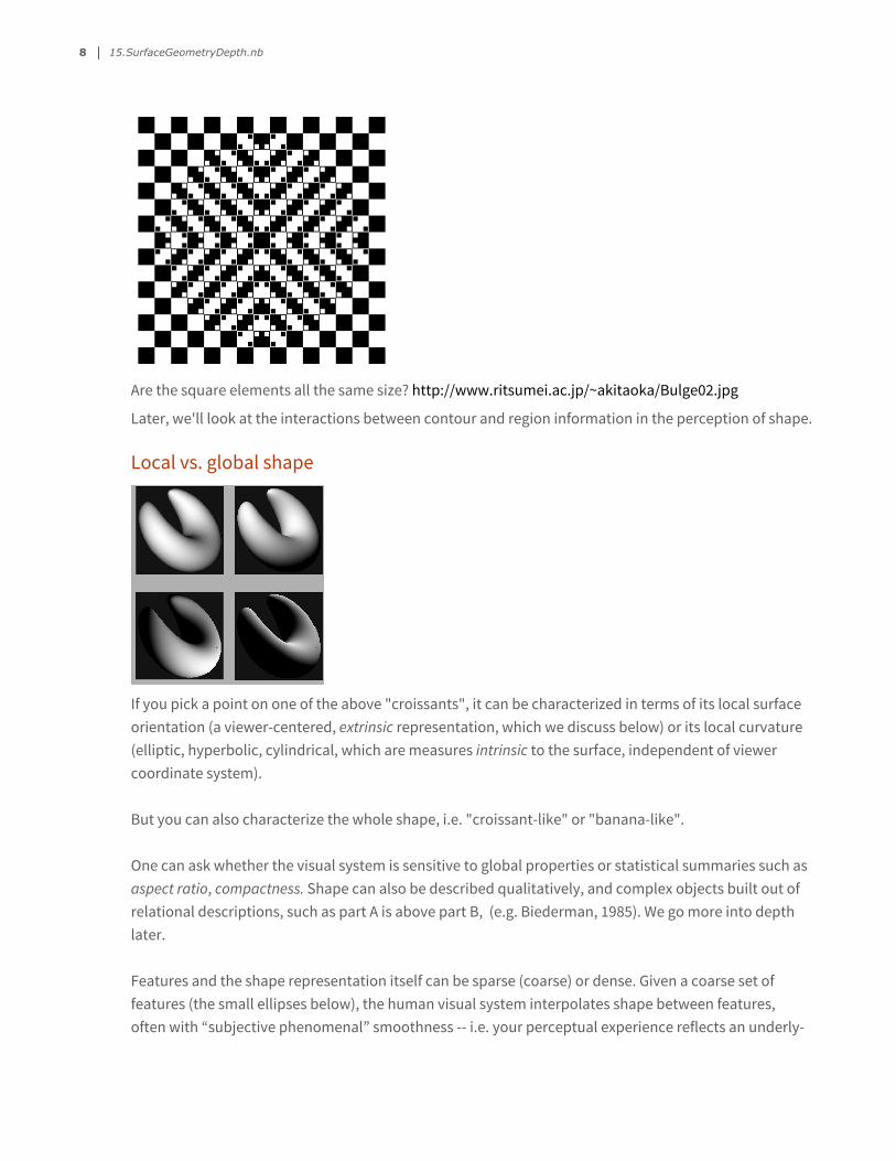
Are the square elements all the same size? http://www.ritsumei.ac.jp/~akitaoka/Bulge02.jpg
Later, we'll look at the interactions between contour and region information in the perception of shape.
Local vs. global shape
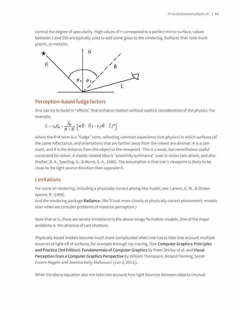
If you pick a point on one of the above "croissants", it can be characterized in terms of its local surface orientation (a viewer-centered, extrinsic representation, which we discuss below) or its local curvature (elliptic, hyperbolic, cylindrical, which are measures intrinsic to the surface, independent of viewer coordinate system).
But you can also characterize the whole shape, i.e. "croissant-like" or "banana-like".
One can ask whether the visual system is sensitive to global properties or statistical summaries such as aspect ratio, compactness. Shape can also be described qualitatively, and complex objects built out of relational descriptions, such as part A is above part B, (e.g. Biederman, 1985). We go more into depth later.
Features and the shape representation itself can be sparse (coarse) or dense. Given a coarse set of features (the small ellipses below), the human visual system interpolates shape between features, often with “subjective phenomenal” smoothness -- i.e. your perceptual experience reflects an underly-ing process of surface interpolation through the features. This is problem is perceptually important and of theoretical interest. How to go from a set of sparse measurements in a region to a dense field? This subject surface interpolation can be quite compelling with motion or stereo cues. We’ll see more of that later.
8 15.SurfaceGeometryDepth.nb
If you pick a point on one of the above "croissants", it can be characterized in terms of its local surface orientation (a viewer-centered, extrinsic representation, which we discuss below) or its local curvature (elliptic, hyperbolic, cylindrical, which are measures intrinsic to the surface, independent of viewer coordinate system).
But you can also characterize the whole shape, i.e. "croissant-like" or "banana-like".
One can ask whether the visual system is sensitive to global properties or statistical summaries such as aspect ratio, compactness. Shape can also be described qualitatively, and complex objects built out of relational descriptions, such as part A is above part B, (e.g. Biederman, 1985). We go more into depth later.
Features and the shape representation itself can be sparse (coarse) or dense. Given a coarse set of features (the small ellipses below), the human visual system interpolates shape between features, often with “subjective phenomenal” smoothness -- i.e. your perceptual experience reflects an underly-ing process of surface interpolation through the features. This is problem is perceptually important and of theoretical interest. How to go from a set of sparse measurements in a region to a dense field? This subject surface interpolation can be quite compelling with motion or stereo cues. We’ll see more of that later.
The shading on the above croissants provides continuous, dense cues.
Local shape fields & dense estimation
From dense depth to shape, normals & curvature
Below we will start with a mathematically simple representation of depth from the viewer: z = f(x,y), and show how to derive a simple dense shape measure in terms of the rate of change of depth from the viewer. This a viewer-centered depth representation. Later, we will discuss intrinsic object shape measures such as surface curvature.
For an example of the interaction between global shape (is it a quadrangle with non-equal interior angles or a rectangle?) and viewpoint see: http://www.michaelbach.de/ot/sze_shepardTables/in-dex.html
Local dense representations of surface regions
Shape-based generative modeling of images:
A basic vision problem is how to infer geometry from photometry. We'll start with a discussion of dense local representation of shape in terms of surface normals, and understand how shape changes influ-ence image intensity changes. And from there, the inverse problem of seeing shape from shading in the next lecture.
All the models in this section are examples of photometric, scene-based generative image models.
There are two aspects to image formation. The first has to do with geometrical manipulations that describe how surface points project to image points (which we will study later via matrix transforma-tions on homogeneous coordinates). The second aspect is the photometric determination of intensity at each image point from a scene description. In order to understand shape from shading, we need to understand the constraints implicit in the forward optics problem of "shading from shape"--i.e. the generative model. Here we can benefit from research in attempts in computer graphics to obtain photorealism.
Image formation constraints can be obtained by understanding how material properties, shape, and illumination interact to form an image. This is part of the field of computer graphics. The quest for physical realism in reasonable computing time is still a challenge in computer graphics (Greenberg, 1999; for eary history, see: Blinn, J. F., 1977; Cook, R., & Torrance, K., 1982).
One of the earliest models is the Lambertian shading equation which describes how intensity is dis-tributed for curved matte surfaces with constant reflectance (e.g. arbitrarily defined as 1):
15.SurfaceGeometryDepth.nb 9
A basic vision problem is how to infer geometry from photometry. We'll start with a discussion of dense local representation of shape in terms of surface normals, and understand how shape changes influ-ence image intensity changes. And from there, the inverse problem of seeing shape from shading in the next lecture.
All the models in this section are examples of photometric, scene-based generative image models.
There are two aspects to image formation. The first has to do with geometrical manipulations that describe how surface points project to image points (which we will study later via matrix transforma-tions on homogeneous coordinates). The second aspect is the photometric determination of intensity at each image point from a scene description. In order to understand shape from shading, we need to understand the constraints implicit in the forward optics problem of "shading from shape"--i.e. the generative model. Here we can benefit from research in attempts in computer graphics to obtain photorealism.
Image formation constraints can be obtained by understanding how material properties, shape, and illumination interact to form an image. This is part of the field of computer graphics. The quest for physical realism in reasonable computing time is still a challenge in computer graphics (Greenberg, 1999; for eary history, see: Blinn, J. F., 1977; Cook, R., & Torrance, K., 1982).
One of the earliest models is the Lambertian shading equation which describes how intensity is dis-tributed for curved matte surfaces with constant reflectance (e.g. arbitrarily defined as 1):
L (x, y) = E⋀ · N⋀ (x, y) (1)
E(x,y) is a vector representing light source direction. If at infinity, it has just two degrees of freedom and is constant over the surface. If light source intensity is normalized, then the E vector is a unit vector. The above expression assumes a light source at infinity. Alternatively its vector length can be used to indicate the strength of the illumination.
Surfaces can have varying reflectance, r(x,y) representing that fraction of light reflected (varying from 0 for a black pigment to 1 for a white pigment), and then the shading equation becomes:
L (x, y) = r (x, y) E⋀ · N⋀ (x, y)
▶ 3. Show that the lambertian model gives brightness constancy “for free”. In other words, show that the retinal illumination is constant as the angle between the light source and surface normal vary.
An example of a simple computer graphics lighting model--"matte" & "plastic" world
An early elaboration of the lambertian model for shading, based in part on physics, and in part on heuristics and "beauty pageant" observations, describes image luminance in terms of ambient, lamber-tian, and specular components:
L = ra Ea + r Ep⋀ · N⋀ + rs R
⋀ · L⋀n
where the lower case r's are the reflectivities (0 means no reflectance of the illumination, and 1 means complete reflectance), and the unit vectors E, N, and L, point in the directions of the light source, surface normal, and viewpoint respectively. Ep and Ea, are the strengths of the point source, and ambient illumination, respectively. R points in the direction that a ray would go if the surface was a
perfect flat mirror, i.e. purely specular. E⋀· N
⋀ ∝ cos(θi) and R
⋀· N
⋀ ∝ cos(θr), where θi and θr are the
angles of incidence and reflection, respectively. For a flat mirror surface, θi = θr.
The form for the specular term, R⋀· L
⋀n
, is due to Phong, who pointed out that n could be used to
control the degree of specularity. High values of n correspond to a perfect mirror surface, values between 1 and 200 are typically used to add some gloss to the rendering. Surfaces then look more plastic, or metallic.
10 15.SurfaceGeometryDepth.nb
where the lower case r's are the reflectivities (0 means no reflectance of the illumination, and 1 means complete reflectance), and the unit vectors E, N, and L, point in the directions of the light source, surface normal, and viewpoint respectively. Ep and Ea, are the strengths of the point source, and ambient illumination, respectively. R points in the direction that a ray would go if the surface was a
perfect flat mirror, i.e. purely specular. E⋀· N
⋀ ∝ cos(θi) and R
⋀· N
⋀ ∝ cos(θr), where θi and θr are the
angles of incidence and reflection, respectively. For a flat mirror surface, θi = θr.
The form for the specular term, R⋀· L
⋀n
, is due to Phong, who pointed out that n could be used to
control the degree of specularity. High values of n correspond to a perfect mirror surface, values between 1 and 200 are typically used to add some gloss to the rendering. Surfaces then look more plastic, or metallic.
Perception-based fudge factors
One can try to build in “effects” that enhance realism without explicit consideration of the physics. For example,
where the R+K term is a "fudge" term, reflecting common experience (not physics) in which surfaces (of the same reflectance, and orientation) that are farther away from the viewer are dimmer. K is a con-stant, and R is the distance from the object to the viewpoint. This is a weak, but nevertheless useful constraint for vision. A closely related idea is "proximity luminance" cues in vision (see above, and also Dosher, B. A., Sperling, G., & Wurst, S. A., 1986). The assumption is that one’s viewpoint is likely to be close to the light source direction than opposite it.
Limitations
For more on rendering, including a physically correct phong-like model, see: Larson, G. W., & Shake-speare, R. (1998).And the rendering package Radiance. (We’ll look more closely at physically correct photometric models later when we consider problems of material perception.)
Note that as is, there are severe limitations to the above image formation models. One of the major problems is the absence of cast shadows.
Physically based models become much more complicated when one has to take into account multiple bounces of light off of surfaces, for example through ray-tracing. (See Computer Graphics: Principles and Practice (3rd Edition); Fundamentals of Computer Graphics by Peter Shirley et al. and Visual Perception from a Computer Graphics Perspective by William Thompson, Roland Fleming, Sarah Creem-Regehr and Jeanine Kelly Stefanucci (Jun 2, 2011)).
While the above equation also not take into account how light bounces between objects (mutual illumination or indirect lighting)--the ambient “fudge” term is the crude approximation to model the overall effect of mutual illumination.
Material properties can be much more complicated than Lambertian plus a Phong specular term. Illumination patterns can also be much more complicated, as illustrated every time you look at a shiny object. More on the complexities of the image formation model later.
15.SurfaceGeometryDepth.nb 11
For more on rendering, including a physically correct phong-like model, see: Larson, G. W., & Shake-speare, R. (1998).And the rendering package Radiance. (We’ll look more closely at physically correct photometric models later when we consider problems of material perception.)
Note that as is, there are severe limitations to the above image formation models. One of the major problems is the absence of cast shadows.
Physically based models become much more complicated when one has to take into account multiple bounces of light off of surfaces, for example through ray-tracing. (See Computer Graphics: Principles and Practice (3rd Edition); Fundamentals of Computer Graphics by Peter Shirley et al. and Visual Perception from a Computer Graphics Perspective by William Thompson, Roland Fleming, Sarah Creem-Regehr and Jeanine Kelly Stefanucci (Jun 2, 2011)).
While the above equation also not take into account how light bounces between objects (mutual illumination or indirect lighting)--the ambient “fudge” term is the crude approximation to model the overall effect of mutual illumination.
Material properties can be much more complicated than Lambertian plus a Phong specular term. Illumination patterns can also be much more complicated, as illustrated every time you look at a shiny object. More on the complexities of the image formation model later.
Preview of the shape-from-shading problem
Later we will study the "shape-from-shading" problem. If one represents shape in terms of a dense distribution of surface normals, then a simplified version of the formal problem is to estimate N(x,y) given data L(x,y) such that the following simplification of the above equations holds:
(2)
As it stands, this set of equations (one for each location x,y) is underconstrained or "ill-posed". Even if we knew the light source direction E, for every image intensity L, there are two numbers to estimate for N. Assuming the light source is a point at infinity simplifies things (same two numbers E for all surface points). Assuming surface smoothness and integrability also constrains the solution. But more on this later. The generative model in equation 2 needs to be supplemented with a prior model on the space of possible surfaces in order to perform inverse inference.
Representing shape: global representations
We pointed out above that a central issue in object perception is how the shape of an object is repre-sented by the visual system. Shape may be represented in a variety of ways that depend on the visual task and the stages of processing in a given task.
Questions about shape representation can be classified along several dimensions. Two central ques-tions have to do with whether the representation is local or global, and whether the representation depends on viewpoint.
Global and local representations of shape. A global representation of solid shape consists of a set of parameters or templates that describe a class of surfaces or ``parts". Several theories of object recogni-tion assume that objects can be decomposed into elementary parts. These parts are drawn from a limited set of elementary shapes, such as generalized cylinders (Marr and Nishihara, 1978), geons (Biederman, 1987) or superquadrics (Pentland, 1990). Shapes can be characterized by their skeletons (e.g. Wilder, J., Feldman, J., & Singh, M., 2011).
Some global representations have the property that a change of one parameter which describes a part will affect the whole shape. An example of this are spline representations.
In comparison, a local representation is a dense characterization of shape, such that a change of a parameter at one spatial location will not affect the shape at another location. A surface normal vector at each surface location is an example of a dense representation.
Viewpoint dependency in shape representations. A second major question is whether the shape represen-tation depends on viewpoint. This debate has arisen in the context of models of object recognition (Tarr & Bülthoff, 1995). Local viewpoint dependent descriptors such as surface normals (or slant and tilt, see below) have an early history (Todd & Mingolla, 1983; Mingolla & Todd, 1986; see below). But view-dependent descriptors have disadvantages for some tasks. One problem with slant and tilt is that the local slant of an oriented plane varies with viewpoint. So we have a discrepancy between apparent global flatness and the local variation in slant (Mamassian, 1995).
For part-based object recognition, it would seem best to do part extraction using local view-indepen-dent descriptors. It is also reasonable that view-independent shape descriptors could support other types of visual processes. For instance, the manual prehension of an object requires one to locate stable grasp points on the surface, a task which only makes sense in an object-centered frame of reference. Nevertheless, the visual information is of course firstly described in a viewer-centered frame of reference, and the fundamental issue then becomes the tranformation of viewpoint dependent into viewpoint independent representation (Andersen, 1987). One local, intrinsic representation of solid shape describes the second order depth variation of the surface (Besl and Jain, 1986), or equivalently, the first order orientation variation (Rogers and Cagenello, 1989). For more on shape representations, see Koenderink (1990).
Compositions. When we discuss the problem of object recognition later in the course, we’ll look at ways of describing objects in terms of “compositions”, in which one builds a global representation from “resuable” features and parts and their relationships. These are sometimes called “structural descrip-tions”. Such descriptions have a number of advantages including the ability to change a part descrip-tion without affecting the whole, and when incorporated into a hierarchical model, the ability to represent a rich set of a semantically meaningful variations.
15.SurfaceGeometryDepth.nb 13
Compositions. When we discuss the problem of object recognition later in the course, we’ll look at ways of describing objects in terms of “compositions”, in which one builds a global representation from “resuable” features and parts and their relationships. These are sometimes called “structural descrip-tions”. Such descriptions have a number of advantages including the ability to change a part descrip-tion without affecting the whole, and when incorporated into a hierarchical model, the ability to represent a rich set of a semantically meaningful variations.
Gradient space & surface normals
Let’s look more closely at local, dense, viewpoint dependent representations. We begin with surface normal representation that we saw above: N(x,y).
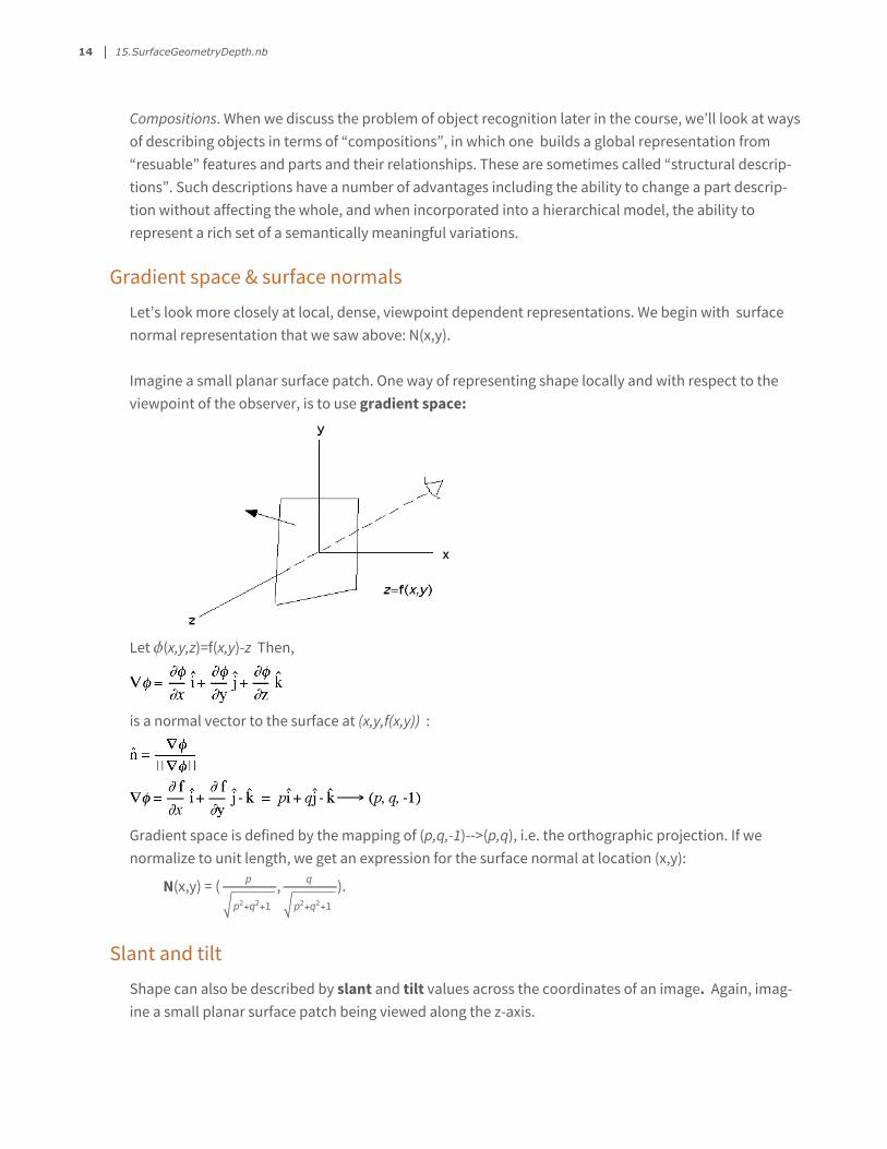
Imagine a small planar surface patch. One way of representing shape locally and with respect to the viewpoint of the observer, is to use gradient space:
Let ϕ(x,y,z)=f(x,y)-z Then,
is a normal vector to the surface at (x,y,f(x,y)) :
Gradient space is defined by the mapping of (p,q,-1)-->(p,q), i.e. the orthographic projection. If we normalize to unit length, we get an expression for the surface normal at location (x,y):
N(x,y) = ( p
p2+q2+1
, q
p2+q2+1
).
Slant and tilt
Shape can also be described by slant and tilt values across the coordinates of an image. Again, imag-ine a small planar surface patch being viewed along the z-axis.
(Note: Sign convention can differ from one study to the next, e.g. whether the viewer is looking from a point on +z or -z.)
14 15.SurfaceGeometryDepth.nb
Shape can also be described by slant and tilt values across the coordinates of an image. Again, imag-ine a small planar surface patch being viewed along the z-axis.
(Note: Sign convention can differ from one study to the next, e.g. whether the viewer is looking from a point on +z or -z.)
Slant and tilt measures are used in perceptual studies of both local dense estimation, and global near-planar surface attributes, e.g. for large-scale layout.
Let N be the (un-normalized) surface normal expressed in terms of p and q:
Here are the important intuitive interpretations.
The slant is the inclination of the surface relative to the viewer and is related to p and q by:
A slant of zero means that the surface is "fronto-parallel".
The tilt is the direction of steepest descent away from the viewer:
Note: Sqrt[q^2+p^2] is the rate of change of z in the direction of maximum change (steepest descent).
How to choose a representation?
How do we know what is the best representation to use? Slant and tilt seem to be important from a perceptual point of view. But one reason gradient space is useful is that it is related to relative depth in a straight forward way.
We can get back to distance by integrating:
gives the relative distance, and a constant is lost in the process.
For examples of perceptual studies of local shape representations see: Koenderink, 1990 (and the many papers/book by him and his group); and also Mamassian & Kersten 1996, Mamassian, Knill & Kersten (1996).
15.SurfaceGeometryDepth.nb 15
gives the relative distance, and a constant is lost in the process.
For examples of perceptual studies of local shape representations see: Koenderink, 1990 (and the many papers/book by him and his group); and also Mamassian & Kersten 1996, Mamassian, Knill & Kersten (1996).
Using Mathematica to go from depth to normals to image intensities using the Lambertian model
This section gives you some practice using the Lambertian scene-based generative model.
Range data defines surface list
Range data to define rface list -- BIG 64x64 file. (Originally from: http://sampl.eng.ohio-state.edu/)
Intensity in a DensityPlot is proportional to the z (depth) from the camera
ReferencesBiederman, I. (1985). Human image understanding: Recent research and a theory. Computer Vision, Graphics, and Image Processing, 32, 29-73.Blake, A., & Bülthoff, H. H. (1990). Does the brain know the physics of specular reflection? Nature, 343, 165-169.Blake, A., & Bülthoff, H. H. (1991). Shape from specularities: Computation and Psychophysics. Philosoph-ical Transactions of the Royal Society (London) Series B, 331, 237-252.Blinn, J. F. (1977). Models of light reflection for computer synthesized pictures. Computer Graphics, 11(2), 192-198.Brady, M., & Yuille, A. (1984). An extremum principle for shape from contour. IEEE Transactions on pattern analysis and machine intelligence, PAMI-6(3), 288-301.Cook, R., & Torrance, K. (1982). A reflectance model for computer graphics. ACM TOB, 1(1), 7-24.)Dosher, B. A., Sperling, G., & Wurst, S. A. (1986). Tradeoffs between stereopsis and proximity luminance covariance as determinants of perceived 3D structure. Vision Research, 26(6), 973-990.Dupuis, P., & Oliensis, J. (1994). An optimal control formulation and related numerical methods for a problem in shape reconstruction. The Annals of Applied Probability, 4(No, 2), 287-346.Engel, S. A., Remus, D. A., & Sainath, R. (2006). Motion from occlusion. Journal of Vision, 6(5), 9–9. http://doi.org/10.1167/6.5.9Fantoni, C., & Gerbino, W. (2003). Contour interpolation by vector-field combination. Journal of Vision, 3(4), 281–303. http://doi.org/10.1167/3.4.4Foley, J. D., van Dam, A., Feiner, S. K., & Hughes, J. F. (1990). Computer Graphics: Principles and Prac-tice (2nd ed.). Reading, Massachusetts. Addison-Wesley.)Freeman, W. T. (1994). The generic viewpoint assumption in a framework for visual perception. Nature, 368(7 April 1994), 542-545.W. T. Freeman, Exploiting the generic viewpoint assumption, International Journal Computer Vision, 20 (3), 243-261, 1996. TR93-15. W. T. Freeman, The generic viewpoint assumption in a Bayesian framework, in Perception as Bayesian Inference, D. Knill and W. Richards, eds., Cambridge University Press, 365 - 390, 1996.Greenberg, D. P. (1989). Light reflection models for computer graphics. Science, 244, 166-173.Greenberg, D. P. (1999 ). A framework for realistic image synthesis. J Commun. ACM, 42(8), 44-53 Hummel, J. E., & Biederman, I. (1992). Dynamic binding in a neural network for shape recognition. Psychological Review, 99(3), 480–517.Ikeuchi, K., & Horn, B. K. P. (1981). Numerical shape from shading and occluding boundaries. Artificial Intelligence, 17,, 141-184.Kersten, D., O'Toole, A. J., Sereno, M. E., Knill, D. C., & Anderson, J. A. (1987). Associative learning of scene parameters from images. Applied Optics, 26, 4999-5006.)Kersten, D. (1999). High-level vision as statistical inference. In M. Gazzaniga (Ed.), The Cognitive Neuro-sciences Cambridge, MA: MIT Press.Knill, D. C., & Kersten, D. (1990). Learning a near-optimal estimator for surface shape from shading. Computer Vision, Graphics and Image Processing., 50(1), 75-100.Koenderink, J. J. (1990). Solid Shape . Cambridge, Massachusetts: M.I.T. Press.Larson, G. W., & Shakespeare, R. (1998). Rendering With Radiance: The Art and Science of Lighting Visualization.Langer, M. S., & Zucker, S. W. (1994). Shape from Shading on a Cloudy Day. Journal of the Optical Society of America A, 11(2), 467-478.Lee, J.C.; , "Hacking the Nintendo Wii Remote," Pervasive Computing, IEEE , vol.7, no.3, pp.39-45, July-Sept. 2008, doi: 10.1109/MPRV.2008.53, URL: http://ieeexplore.ieee.org/stamp/stamp.jsp?tp=&arnum-ber=4563908&isnumber=4563896Lehky, S. R., & Sejnowski, T. J. (1988). Network model of shape from shading: neural function arises from both receptive and projective fields. Nature, 333, 452-454.Loomis, J. M., Da Silva, J. A., Fujita, N., & Fukusima, S. S. (1992). Visual space perception and visually directed action. J Exp Psychol Hum Percept Perform, 18(4), 906-921.Mamassian, P., & Kersten, D. (1996). Illumination, shading and the perception of local orientation. Vision Res, 36(15), 2351-2367.Mamassian, P., Kersten, D., & Knill, D. C. (1996). Categorical local-shape perception. Perception, 25(1), 95-107.Marotta, J. J., & Goodale, M. A. (2001). Role of familiar size in the control of grasping. J Cogn Neurosci, 13(1), 8-17.Mingolla, E., & Todd, J. T. (1986). Perception of Solid Shape from Shading. 53, 137-151.Nakayama, K., & Shimojo, S. (1992). Experiencing and perceiving visual surfaces. Science, 257, 1357-1363.Oliensis, J. (1991). Uniqueness in Shape From Shading. The International Journal of Computer Vision, 6(2), 75-104.Ramachandran, V. S. (1988). Perceiving Shape from Shading. Scientific American, , 76-83.Shirley, Peter, Michael Ashikhmin, Michael Gleicher, Stephen R. Marschner, Erik Reinhard, Kelvin Sung, William B. Thompson, Peter Willemsen (2005) . Fundamentals of Computer Graphics. 2nd edition.Tarr, M. J., & Bülthoff, H. H. (1995). Is human object recognition better described by geon-structural-descriptions or by multiple-views? Journal of Experimental Psychology: Human Perception and Perfor-mance, 21(6), 1494-1505.Thompson, William, Roland Fleming, Sarah Creem-Regehr and Jeanine Kelly Stefanucci (2011). Visual Perception from a Computer Graphics Perspective Todd, J. T., & Mingolla, E. (1983). Perception of Surface Curvature and Direction of Illumination from Patterns of Shading. Journal of Experimental Psychology: Human Perception & Performance, 9(4), 583-595.Todd, J. T., Norman, J. F., Koenderink, J. J., & Kappers, A. M. L. (1997). Effects of texture, illumination, and surface reflectance on stereoscopic shape perception. Perception, 26(7), 807-822.Todd, J. T., & Reichel, F. D. (1989). Ordinal structure in the visual perception and cognition of smoothly curved surfaces. Psychological Review, 96(4), 643-657.Yuille, A. L., & Bülthoff, H. H. (1996). Bayesian decision theory and psychophysics. In K. D.C., & R. W. (Ed.), Perception as Bayesian Inference Cambridge, U.K.: Cambridge University Press.Wilder, J., Feldman, J., & Singh, M. (2011). Superordinate shape classification using natural shape statistics. COGNITION, 119(3), 325–340. doi:10.1016/j.cognition.2011.01.009
15.SurfaceGeometryDepth.nb 19
Biederman, I. (1985). Human image understanding: Recent research and a theory. Computer Vision, Graphics, and Image Processing, 32, 29-73.Blake, A., & Bülthoff, H. H. (1990). Does the brain know the physics of specular reflection? Nature, 343, 165-169.Blake, A., & Bülthoff, H. H. (1991). Shape from specularities: Computation and Psychophysics. Philosoph-ical Transactions of the Royal Society (London) Series B, 331, 237-252.Blinn, J. F. (1977). Models of light reflection for computer synthesized pictures. Computer Graphics, 11(2), 192-198.Brady, M., & Yuille, A. (1984). An extremum principle for shape from contour. IEEE Transactions on pattern analysis and machine intelligence, PAMI-6(3), 288-301.Cook, R., & Torrance, K. (1982). A reflectance model for computer graphics. ACM TOB, 1(1), 7-24.)Dosher, B. A., Sperling, G., & Wurst, S. A. (1986). Tradeoffs between stereopsis and proximity luminance covariance as determinants of perceived 3D structure. Vision Research, 26(6), 973-990.Dupuis, P., & Oliensis, J. (1994). An optimal control formulation and related numerical methods for a problem in shape reconstruction. The Annals of Applied Probability, 4(No, 2), 287-346.Engel, S. A., Remus, D. A., & Sainath, R. (2006). Motion from occlusion. Journal of Vision, 6(5), 9–9. http://doi.org/10.1167/6.5.9Fantoni, C., & Gerbino, W. (2003). Contour interpolation by vector-field combination. Journal of Vision, 3(4), 281–303. http://doi.org/10.1167/3.4.4Foley, J. D., van Dam, A., Feiner, S. K., & Hughes, J. F. (1990). Computer Graphics: Principles and Prac-tice (2nd ed.). Reading, Massachusetts. Addison-Wesley.)Freeman, W. T. (1994). The generic viewpoint assumption in a framework for visual perception. Nature, 368(7 April 1994), 542-545.W. T. Freeman, Exploiting the generic viewpoint assumption, International Journal Computer Vision, 20 (3), 243-261, 1996. TR93-15. W. T. Freeman, The generic viewpoint assumption in a Bayesian framework, in Perception as Bayesian Inference, D. Knill and W. Richards, eds., Cambridge University Press, 365 - 390, 1996.Greenberg, D. P. (1989). Light reflection models for computer graphics. Science, 244, 166-173.Greenberg, D. P. (1999 ). A framework for realistic image synthesis. J Commun. ACM, 42(8), 44-53 Hummel, J. E., & Biederman, I. (1992). Dynamic binding in a neural network for shape recognition. Psychological Review, 99(3), 480–517.Ikeuchi, K., & Horn, B. K. P. (1981). Numerical shape from shading and occluding boundaries. Artificial Intelligence, 17,, 141-184.Kersten, D., O'Toole, A. J., Sereno, M. E., Knill, D. C., & Anderson, J. A. (1987). Associative learning of scene parameters from images. Applied Optics, 26, 4999-5006.)Kersten, D. (1999). High-level vision as statistical inference. In M. Gazzaniga (Ed.), The Cognitive Neuro-sciences Cambridge, MA: MIT Press.Knill, D. C., & Kersten, D. (1990). Learning a near-optimal estimator for surface shape from shading. Computer Vision, Graphics and Image Processing., 50(1), 75-100.Koenderink, J. J. (1990). Solid Shape . Cambridge, Massachusetts: M.I.T. Press.Larson, G. W., & Shakespeare, R. (1998). Rendering With Radiance: The Art and Science of Lighting Visualization.Langer, M. S., & Zucker, S. W. (1994). Shape from Shading on a Cloudy Day. Journal of the Optical Society of America A, 11(2), 467-478.Lee, J.C.; , "Hacking the Nintendo Wii Remote," Pervasive Computing, IEEE , vol.7, no.3, pp.39-45, July-Sept. 2008, doi: 10.1109/MPRV.2008.53, URL: http://ieeexplore.ieee.org/stamp/stamp.jsp?tp=&arnum-ber=4563908&isnumber=4563896Lehky, S. R., & Sejnowski, T. J. (1988). Network model of shape from shading: neural function arises from both receptive and projective fields. Nature, 333, 452-454.Loomis, J. M., Da Silva, J. A., Fujita, N., & Fukusima, S. S. (1992). Visual space perception and visually directed action. J Exp Psychol Hum Percept Perform, 18(4), 906-921.Mamassian, P., & Kersten, D. (1996). Illumination, shading and the perception of local orientation. Vision Res, 36(15), 2351-2367.Mamassian, P., Kersten, D., & Knill, D. C. (1996). Categorical local-shape perception. Perception, 25(1), 95-107.Marotta, J. J., & Goodale, M. A. (2001). Role of familiar size in the control of grasping. J Cogn Neurosci, 13(1), 8-17.Mingolla, E., & Todd, J. T. (1986). Perception of Solid Shape from Shading. 53, 137-151.Nakayama, K., & Shimojo, S. (1992). Experiencing and perceiving visual surfaces. Science, 257, 1357-1363.Oliensis, J. (1991). Uniqueness in Shape From Shading. The International Journal of Computer Vision, 6(2), 75-104.Ramachandran, V. S. (1988). Perceiving Shape from Shading. Scientific American, , 76-83.Shirley, Peter, Michael Ashikhmin, Michael Gleicher, Stephen R. Marschner, Erik Reinhard, Kelvin Sung, William B. Thompson, Peter Willemsen (2005) . Fundamentals of Computer Graphics. 2nd edition.Tarr, M. J., & Bülthoff, H. H. (1995). Is human object recognition better described by geon-structural-descriptions or by multiple-views? Journal of Experimental Psychology: Human Perception and Perfor-mance, 21(6), 1494-1505.Thompson, William, Roland Fleming, Sarah Creem-Regehr and Jeanine Kelly Stefanucci (2011). Visual Perception from a Computer Graphics Perspective Todd, J. T., & Mingolla, E. (1983). Perception of Surface Curvature and Direction of Illumination from Patterns of Shading. Journal of Experimental Psychology: Human Perception & Performance, 9(4), 583-595.Todd, J. T., Norman, J. F., Koenderink, J. J., & Kappers, A. M. L. (1997). Effects of texture, illumination, and surface reflectance on stereoscopic shape perception. Perception, 26(7), 807-822.Todd, J. T., & Reichel, F. D. (1989). Ordinal structure in the visual perception and cognition of smoothly curved surfaces. Psychological Review, 96(4), 643-657.Yuille, A. L., & Bülthoff, H. H. (1996). Bayesian decision theory and psychophysics. In K. D.C., & R. W. (Ed.), Perception as Bayesian Inference Cambridge, U.K.: Cambridge University Press.Wilder, J., Feldman, J., & Singh, M. (2011). Superordinate shape classification using natural shape statistics. COGNITION, 119(3), 325–340. doi:10.1016/j.cognition.2011.01.009