Copyright: Chandrajit Bajaj, CCV, University of Texas at Austin o m p u t a t i o n a l sualization Cente r CCV Mannheim Summer School 2002 Computational Visualization 1.Sources, characteristics, representation 2.Mesh Processing 3.Contouring 4.Volume Rendering 5.Flow, Vector, Tensor Field Visualization
Transcript
Copyright: Chandrajit Bajaj, CCV, University of Texas at Austin
ComputationalVisualization
Cent
er
CCV Mannheim Summer School 2002
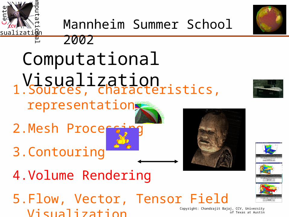
Computational Visualization
1. Sources, characteristics, representation
2. Mesh Processing
3. Contouring
4. Volume Rendering
5. Flow, Vector, Tensor Field Visualization
6. Application Case Studies
Copyright: Chandrajit Bajaj, CCV, University of Texas at Austin
ComputationalVisualization
Cent
er
CCV
Computational Visualization:Volume Rendering
Lecture 4
Copyright: Chandrajit Bajaj, CCV, University of Texas at Austin
ComputationalVisualization
Cent
er
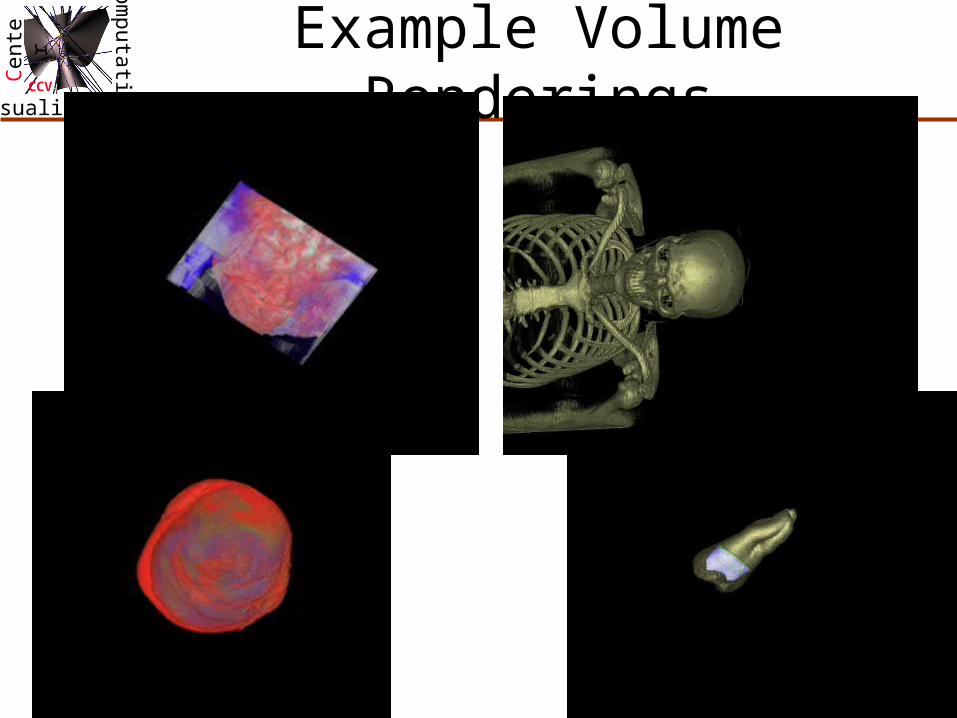
CCVExample Volume Renderings
Copyright: Chandrajit Bajaj, CCV, University of Texas at Austin
ComputationalVisualization
Cent
er
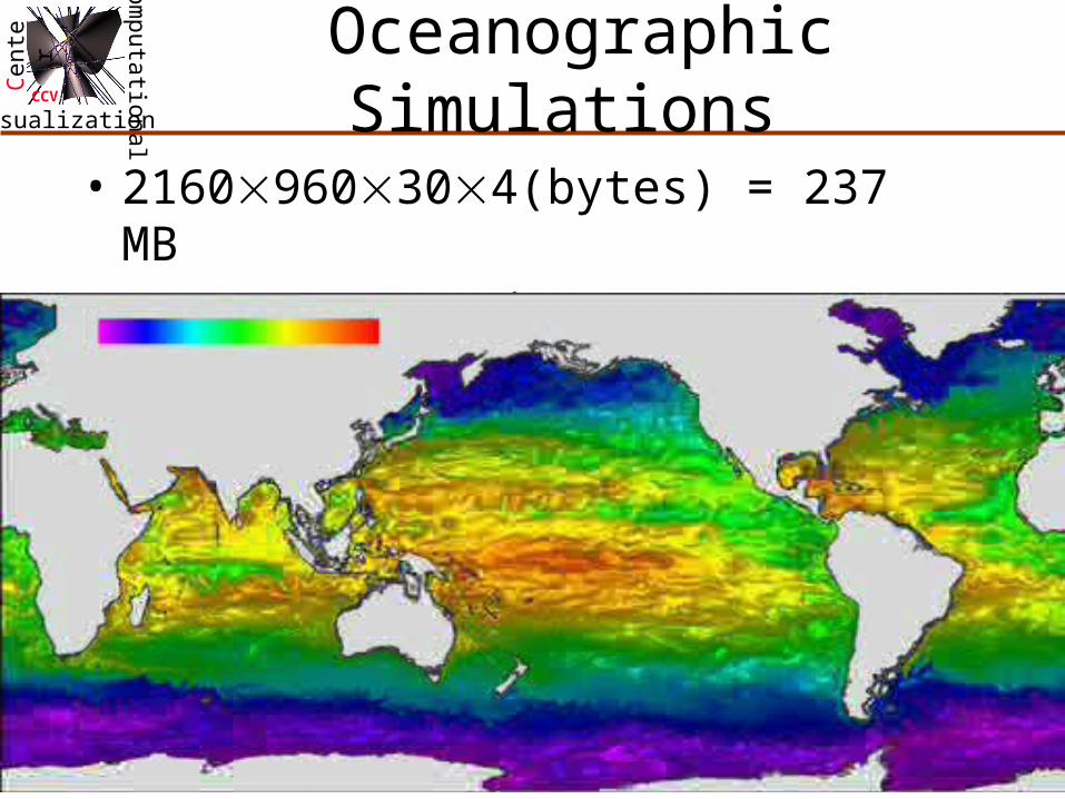
CCVOceanographic Simulations
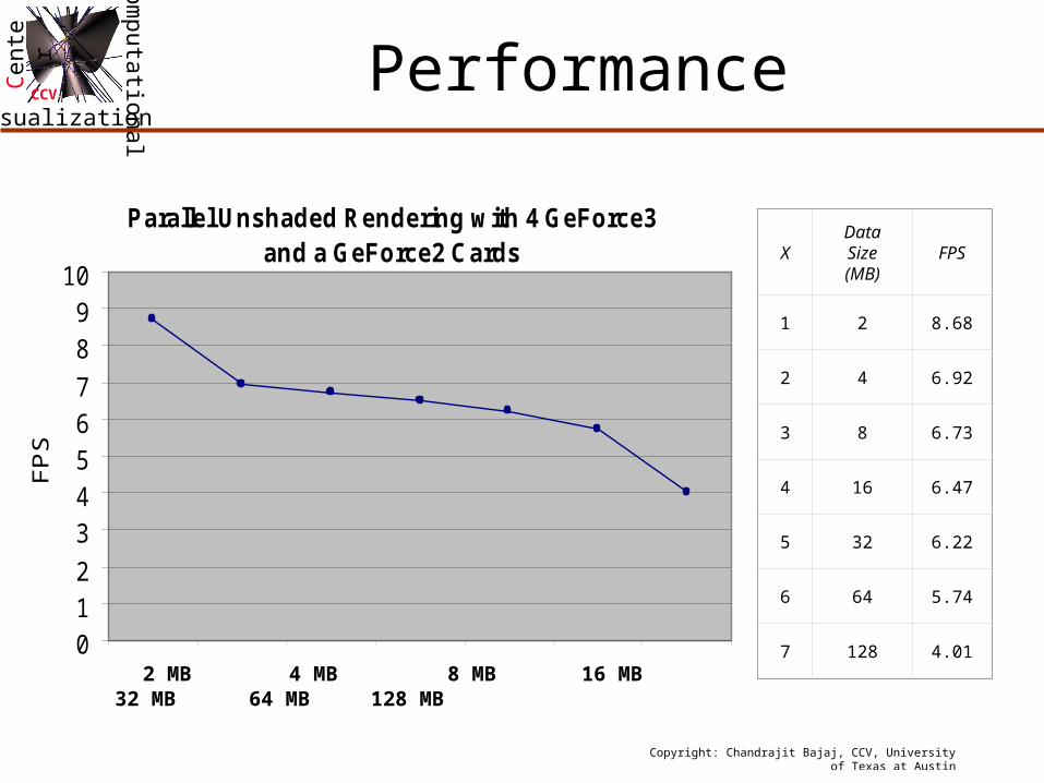
• 2160960304(bytes) = 237 MB
• 237(MB)115(timesteps) = 27 GB
Copyright: Chandrajit Bajaj, CCV, University of Texas at Austin
ComputationalVisualization
Cent
er
CCVOutline
• Ray Casting/Shading
• Opacity weighted Color Integration
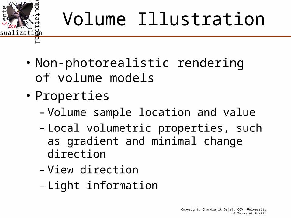
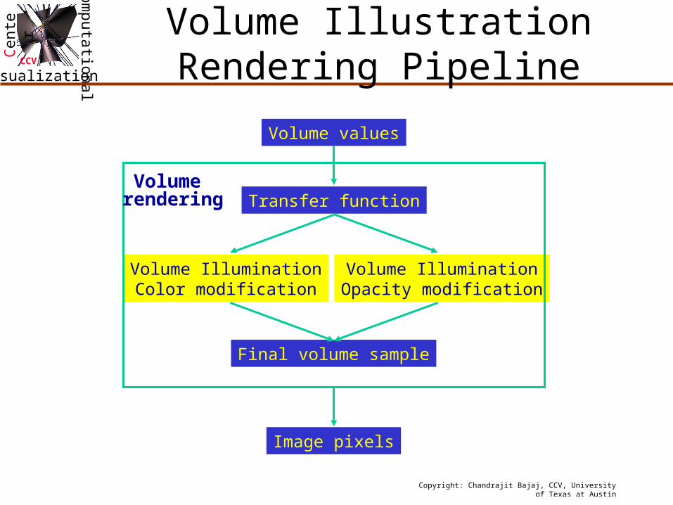
• Volumetric Illustration
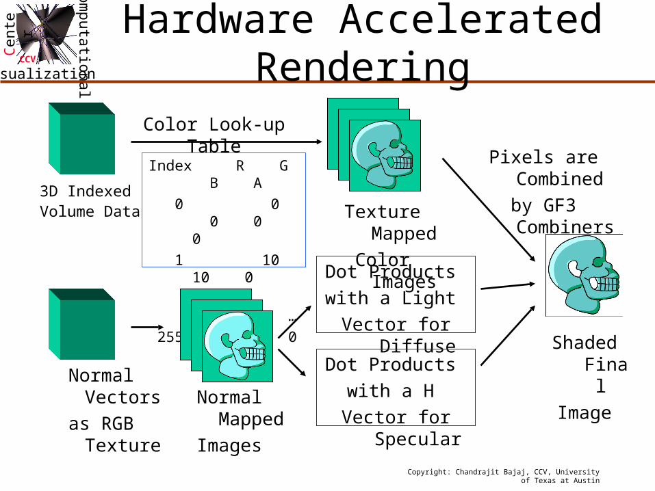
• Texture Based Rendering (Hardware Acceleration)
• Optical Models (Gaseous Phenomena)
First Principles
Copyright: Chandrajit Bajaj, CCV, University of Texas at Austin
ComputationalVisualization
Cent
er
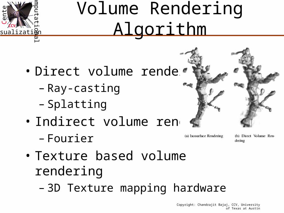
CCVVolume Rendering Algorithm
• Direct volume rendering– Ray-casting– Splatting
• Indirect volume rendering– Fourier
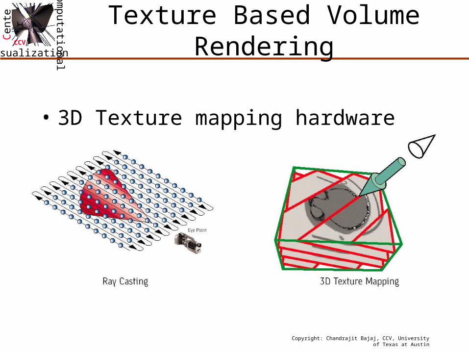
• Texture based volume rendering– 3D Texture mapping hardware
Copyright: Chandrajit Bajaj, CCV, University of Texas at Austin
ComputationalVisualization
Cent
er
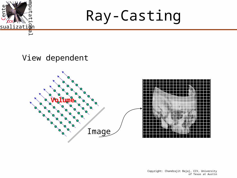
CCVRay-Casting
Image
Volume
View dependent
Copyright: Chandrajit Bajaj, CCV, University of Texas at Austin
ComputationalVisualization
Cent
er
CCVRay-Casting (cont)
• Advantages– Not necessary to explicitly extract surfaces
from volume when rendering– Can change the transfer functions to make
various surfaces stand out within the volume
Copyright: Chandrajit Bajaj, CCV, University of Texas at Austin
ComputationalVisualization
Cent
er
CCVRay-Casting (cont)
• Disadvantages– Do not have explicit representations for
surfaces, therefore not straightforward to compute integral/differential properties
– Much more computationally intensive to render volume since not dealing directly with the efficient polygon pipeline
Copyright: Chandrajit Bajaj, CCV, University of Texas at Austin
ComputationalVisualization
Cent
er
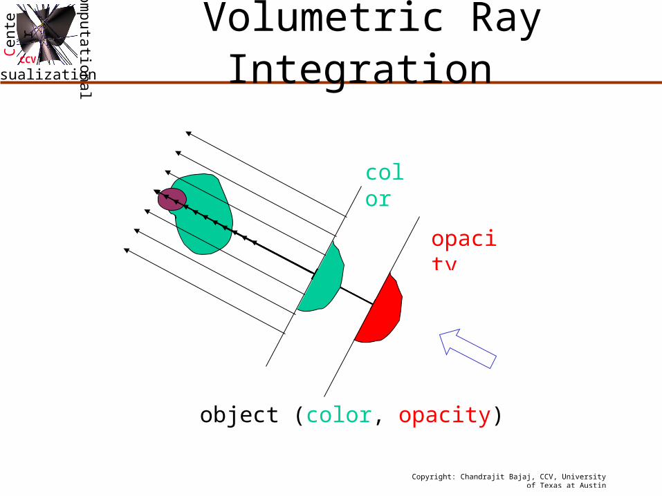
CCV Volumetric Ray Integration
color
opacity
object (color, opacity)
1.0
Copyright: Chandrajit Bajaj, CCV, University of Texas at Austin
ComputationalVisualization
Cent
er
CCV
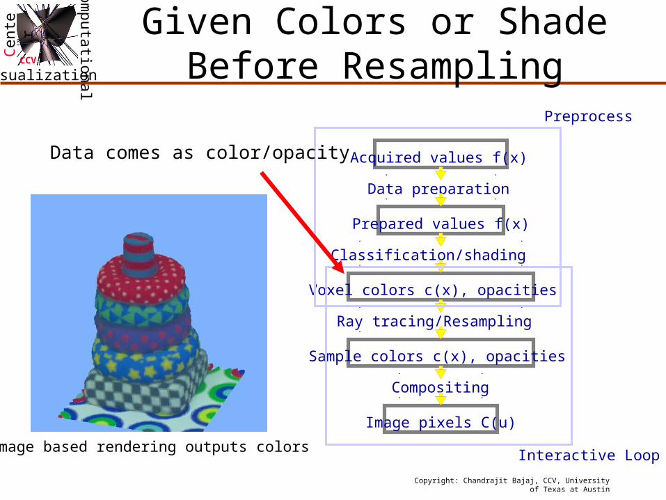
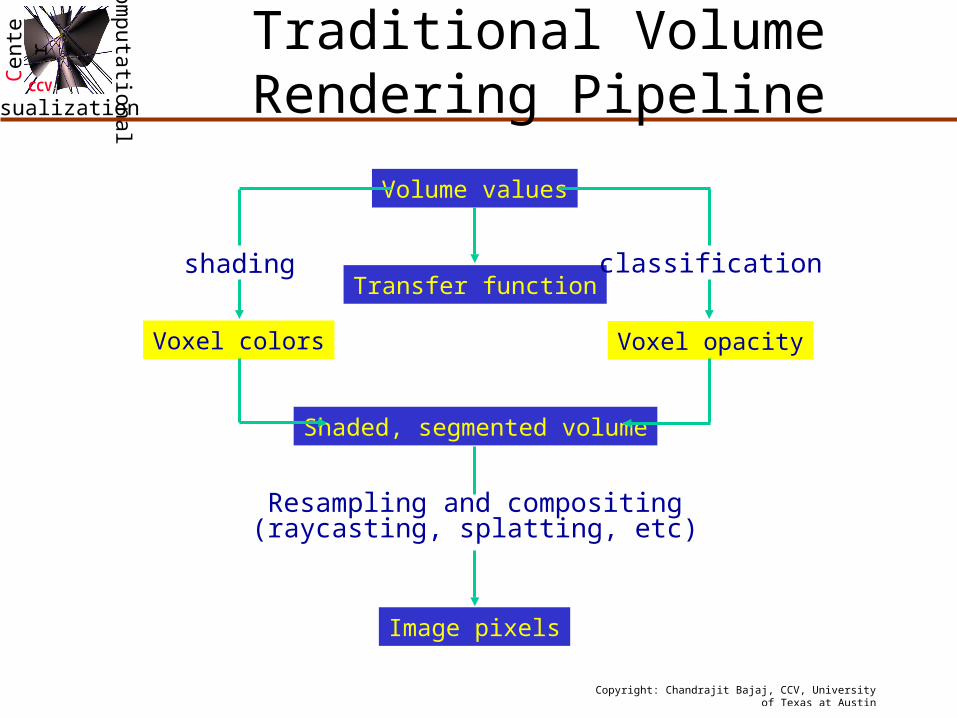
Given Colors or Shade Before Resampling
Sample colors c(x), opacities
Ray tracing/Resampling
Acquired values f(x)
Prepared values f(x)
Voxel colors c(x), opacities
Image pixels C(u)
Data preparation
Classification/shading
Compositing
Preprocess
Interactive LoopImage based rendering outputs colors
Data comes as color/opacity
Copyright: Chandrajit Bajaj, CCV, University of Texas at Austin
ComputationalVisualization
Cent
er
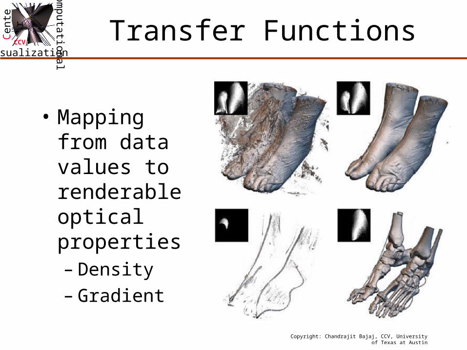
CCVTransfer Functions
• Mapping from data values to renderable optical properties– Density– Gradient
Copyright: Chandrajit Bajaj, CCV, University of Texas at Austin
ComputationalVisualization
Cent
er
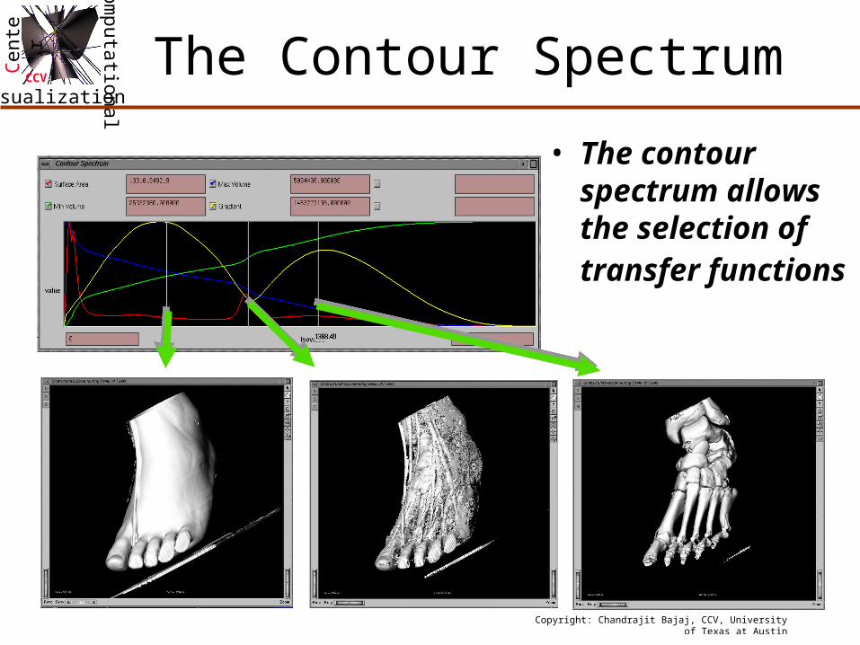
CCV
• The contour spectrum allows the selection of transfer functions
The Contour Spectrum
Copyright: Chandrajit Bajaj, CCV, University of Texas at Austin
ComputationalVisualization
Cent
er
CCV
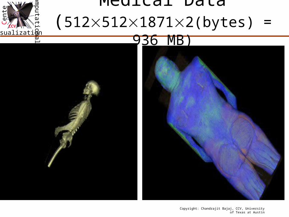
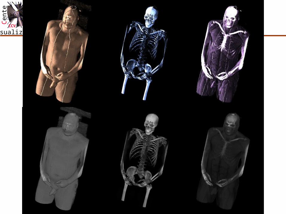
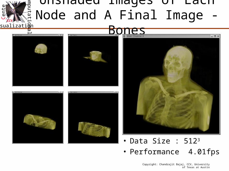
Medical Data(51251218712(bytes) = 936 MB)
Copyright: Chandrajit Bajaj, CCV, University of Texas at Austin
ComputationalVisualization
Cent
er
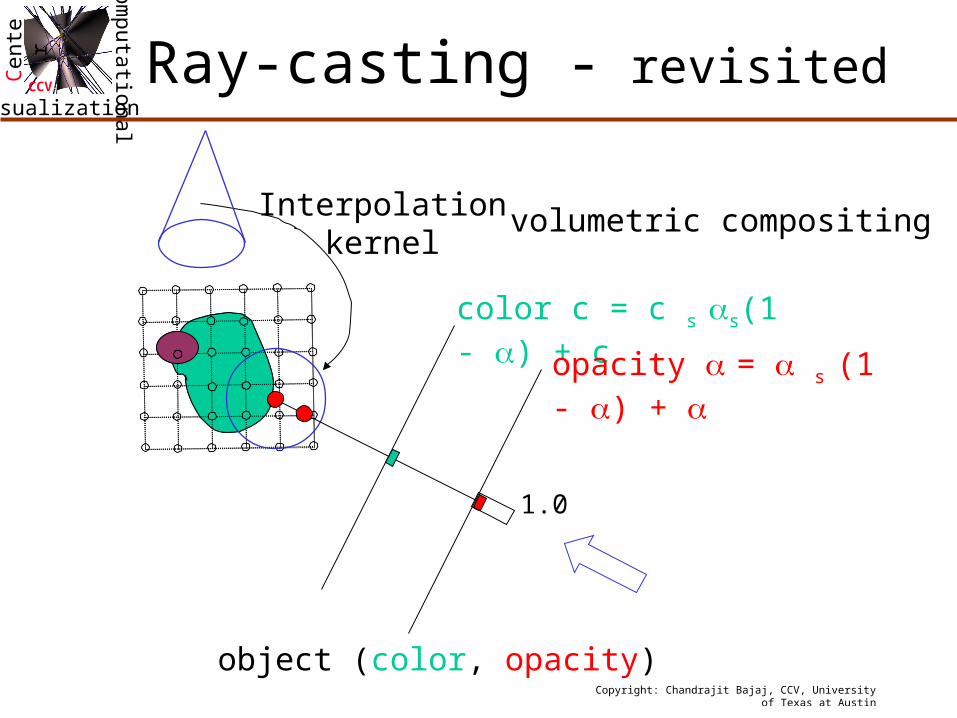
CCVRay-casting - revisited
color c = c s s(1 - ) + c
opacity = s (1 - ) +
1.0
object (color, opacity)
volumetric compositingInterpolationkernel
Copyright: Chandrajit Bajaj, CCV, University of Texas at Austin
ComputationalVisualization
Cent
er
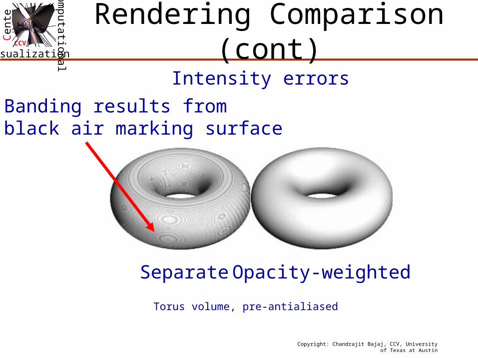
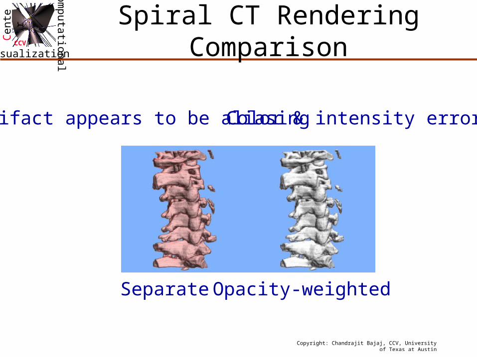
CCVOpacity-Weighted Color
1. From first principles, emitted intensity different from shaded intensity
2. From Blinn, Opacity-Weighting before interpolation helps quality
3. From short cut, cannot do separate interpolation
Copyright: Chandrajit Bajaj, CCV, University of Texas at Austin
ComputationalVisualization
Cent
er
CCV
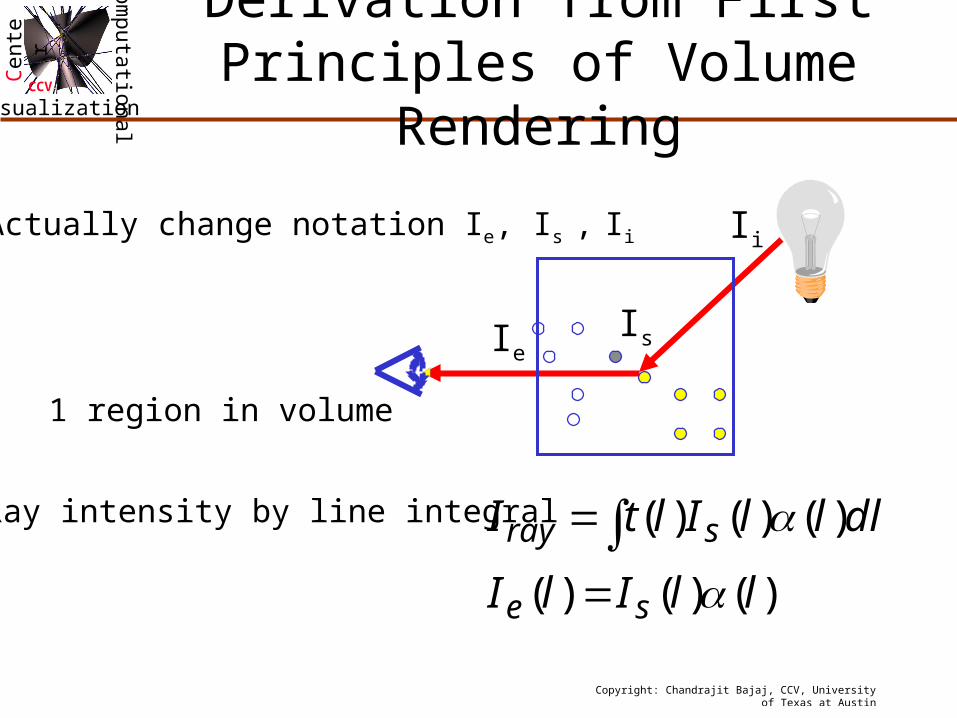
Derivation from First Principles of Volume Rendering
Ii
IsIe
dlllIltI sray )()()(
)()()( llIlI se
•Actually change notation Ie, Is , Ii
Ray intensity by line integral
1 region in volume
Copyright: Chandrajit Bajaj, CCV, University of Texas at Austin
ComputationalVisualization
Cent
er
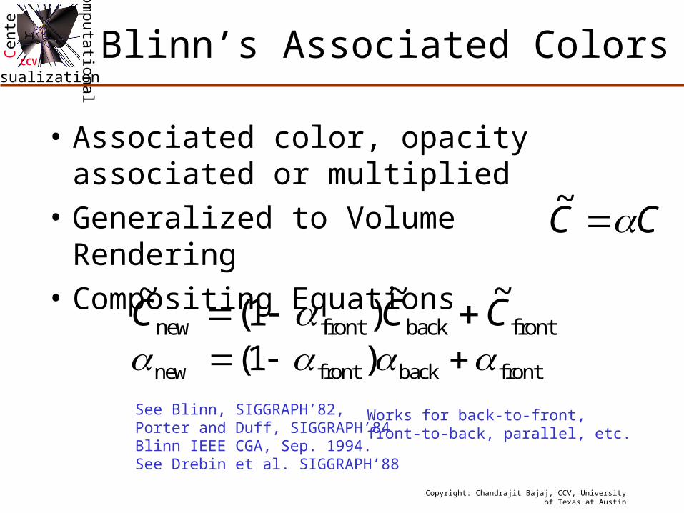
CCVBlinn’s Associated Colors
• Associated color, opacity associated or multiplied
• Generalized to Volume Rendering
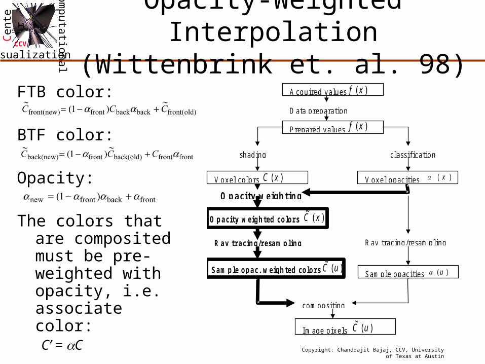
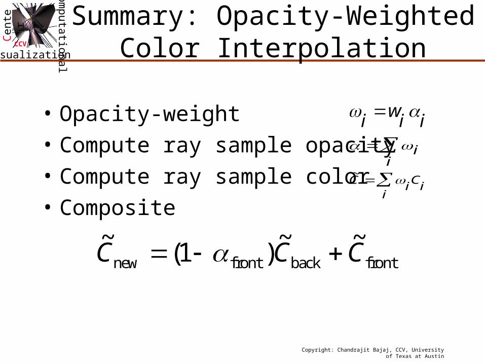
• Compositing Equations~
( )~ ~
C C Cnew front back front 1 new front back front ( )1
~C C
See Blinn, SIGGRAPH’82,Porter and Duff, SIGGRAPH’84Blinn IEEE CGA, Sep. 1994.See Drebin et al. SIGGRAPH’88
Works for back-to-front,front-to-back, parallel, etc.
Copyright: Chandrajit Bajaj, CCV, University of Texas at Austin
ComputationalVisualization
Cent
er
CCV
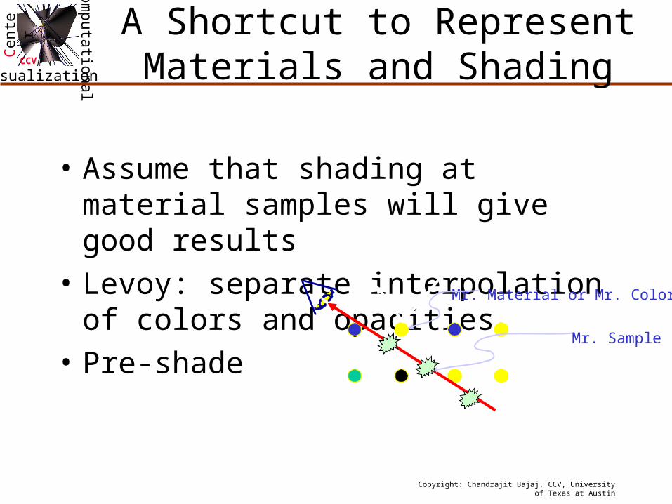
A Shortcut to Represent Materials and Shading
• Assume that shading at material samples will give good results
• Levoy: separate interpolation of colors and opacities
• Pre-shadeMr. Material or Mr. Color
Mr. Sample
Copyright: Chandrajit Bajaj, CCV, University of Texas at Austin
ComputationalVisualization
Cent
er
CCV
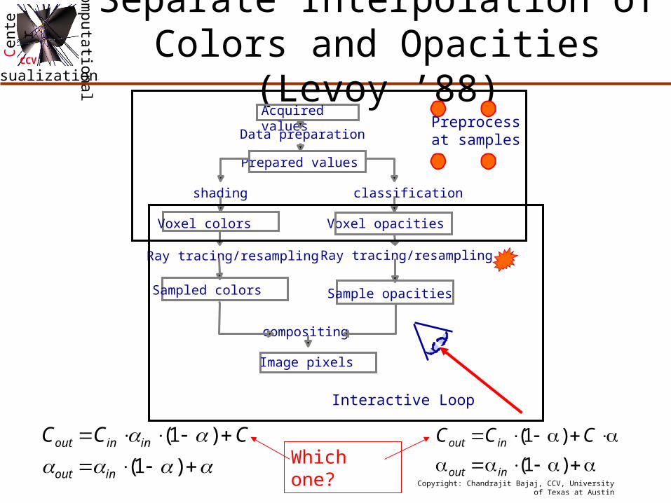
Separate Interpolation of Colors and Opacities (Levoy ’88)
Sample opacities
Voxel opacities
Prepared values
Image pixels
Acquired valuesData preparation
compositing
classification
Ray tracing/resampling
Voxel colors
Sampled colors
shading
Ray tracing/resampling
Preprocessat samples
Interactive Loop
)1(
)1(
inout
inout CCC
)1(
)1(
inout
ininout CCCWhich one?
Copyright: Chandrajit Bajaj, CCV, University of Texas at Austin
ComputationalVisualization
Cent
er
CCV
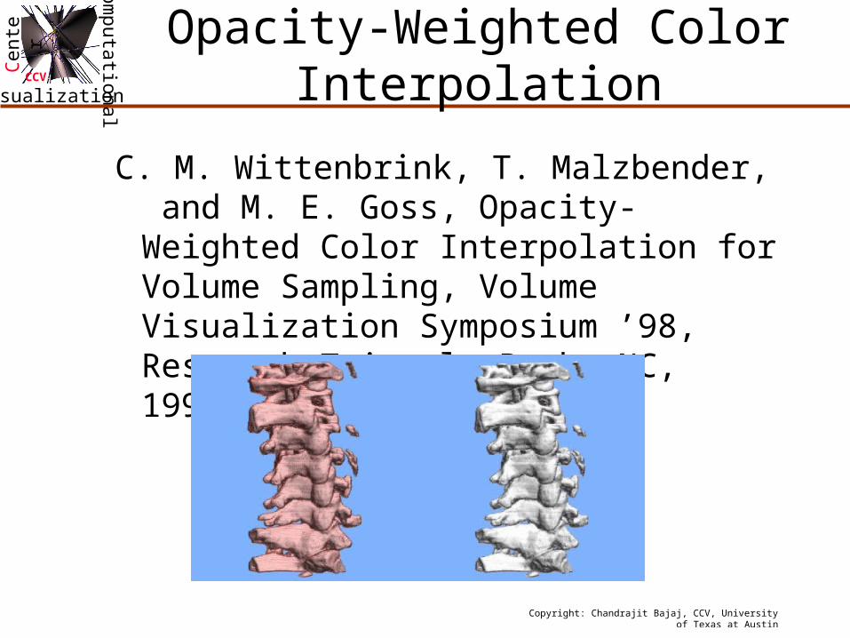
Opacity-Weighted Color Interpolation
C. M. Wittenbrink, T. Malzbender, and M. E. Goss, Opacity-Weighted Color Interpolation for Volume Sampling, Volume Visualization Symposium ’98, Research Triangle Park, NC, 1998.
Copyright: Chandrajit Bajaj, CCV, University of Texas at Austin
Copyright: Chandrajit Bajaj, CCV, University of Texas at Austin
ComputationalVisualization
Cent
er
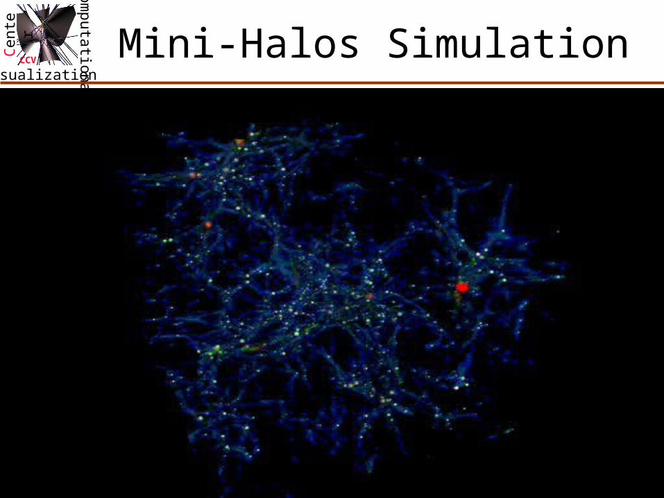
CCVMini-Halos Simulation
Copyright: Chandrajit Bajaj, CCV, University of Texas at Austin
ComputationalVisualization
Cent
er
CCVOptical Models
• Jim Blinn’s 1982 SIGGRAPH paper on light scattering
• Nelson Max, “Optical Models”, IEEE Transactions on Visualization and Computer Graphics, Vol. 1, No. 2, 1995.
• The mathematical framework for light transport in volume rendering based on
S. Chandrasekhar “Radiative Transfer”, Oxford Universtiy Press, 1950
Copyright: Chandrajit Bajaj, CCV, University of Texas at Austin
ComputationalVisualization
Cent
er
CCVTransport of Light
• Determination of Intensity• Local - Diffuse and Specular• Global - Radiosity, Ray Tracing• Mechanisms in Ultimate Model
– Emittance– Absorption– Scattering (single vs. multiple)
Light
Observer
Copyright: Chandrajit Bajaj, CCV, University of Texas at Austin
ComputationalVisualization
Cent
er
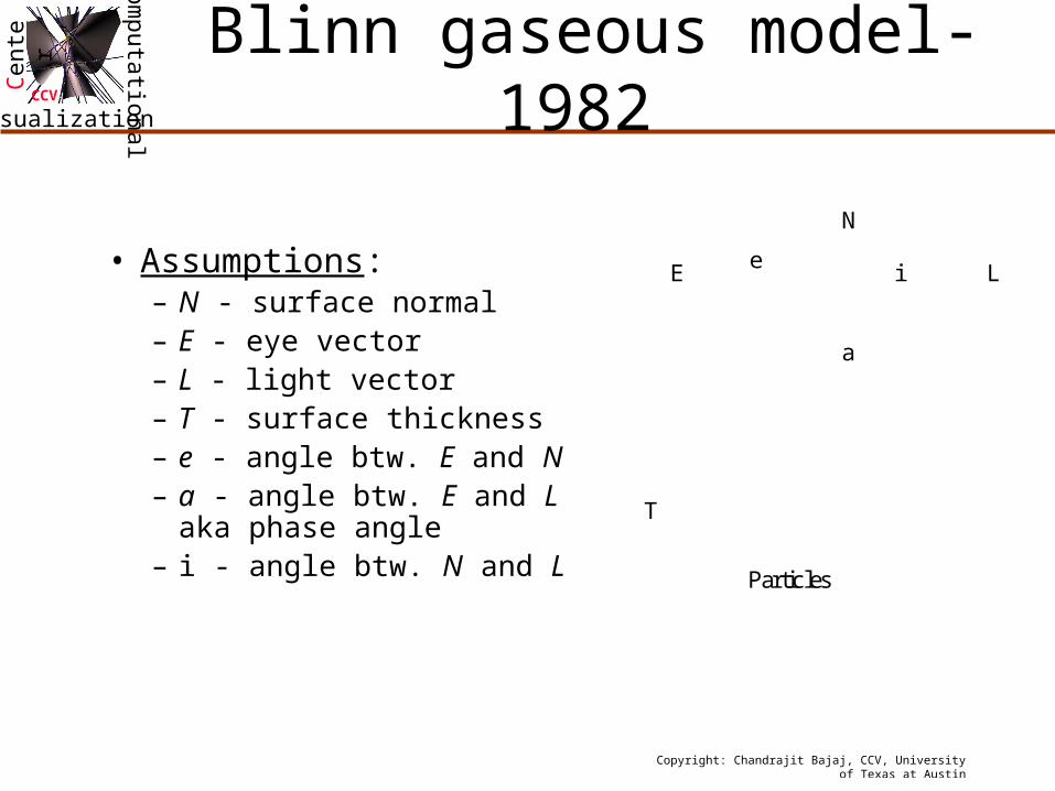
CCVBlinn gaseous model- 1982
• Assumptions:– N - surface normal– E - eye vector– L - light vector– T - surface thickness– e - angle btw. E and N– a - angle btw. E and L
aka phase angle– i - angle btw. N and L
a
LE
N
ei
Particles
T
Copyright: Chandrajit Bajaj, CCV, University of Texas at Austin
ComputationalVisualization
Cent
er
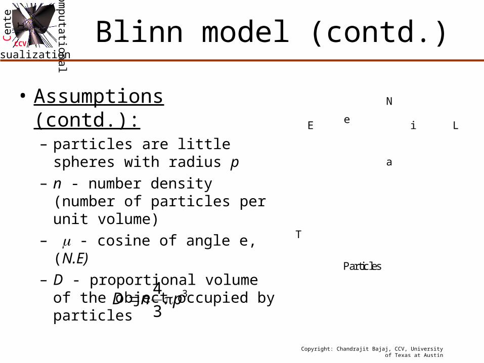
CCVBlinn model (contd.)
• Assumptions (contd.):– particles are little spheres with
radius p– n - number density (number of
particles per unit volume)– - cosine of angle e, (N.E) – D - proportional volume of the
object occupied by particles
a
LE
N
ei
Particles
T
3
3
4pnD
Copyright: Chandrajit Bajaj, CCV, University of Texas at Austin
ComputationalVisualization
Cent
er
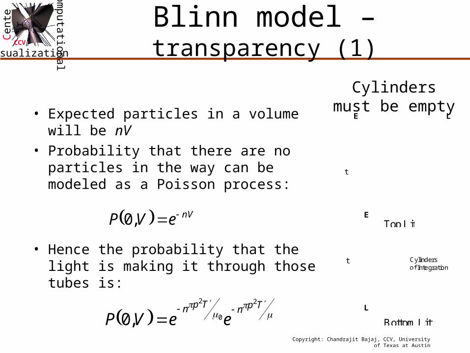
CCVBlinn model – transparency (1)
• Expected particles in a volume will be nV
• Probability that there are no particles in the way can be modeled as a Poisson process:
• Hence the probability that the light is making it through those tubes is:
E L
t
Cylindersmust be empty
nVeVP ,0 E
L
Cylindersof Integration
t
Bottom Lit
Top Lit
TpnTpn
eeVP
2
0
2
,0
Copyright: Chandrajit Bajaj, CCV, University of Texas at Austin
ComputationalVisualization
Cent
er
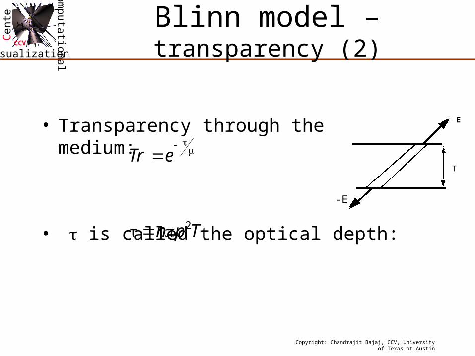
CCVBlinn model – transparency (2)
• Transparency through the medium:
• is called the optical depth:
eTr
E
-E
Tpn 2
T
Copyright: Chandrajit Bajaj, CCV, University of Texas at Austin
ComputationalVisualization
Cent
er
CCVMax model - 1995
• Several cases:– Completely opaque or transparent voxels– Variable opacity correction– Self-emitting glow– Self-emitting glow with opacity along viewing ray– Single scattering of external illumination– Multiple scattering
Copyright: Chandrajit Bajaj, CCV, University of Texas at Austin
ComputationalVisualization
Cent
er
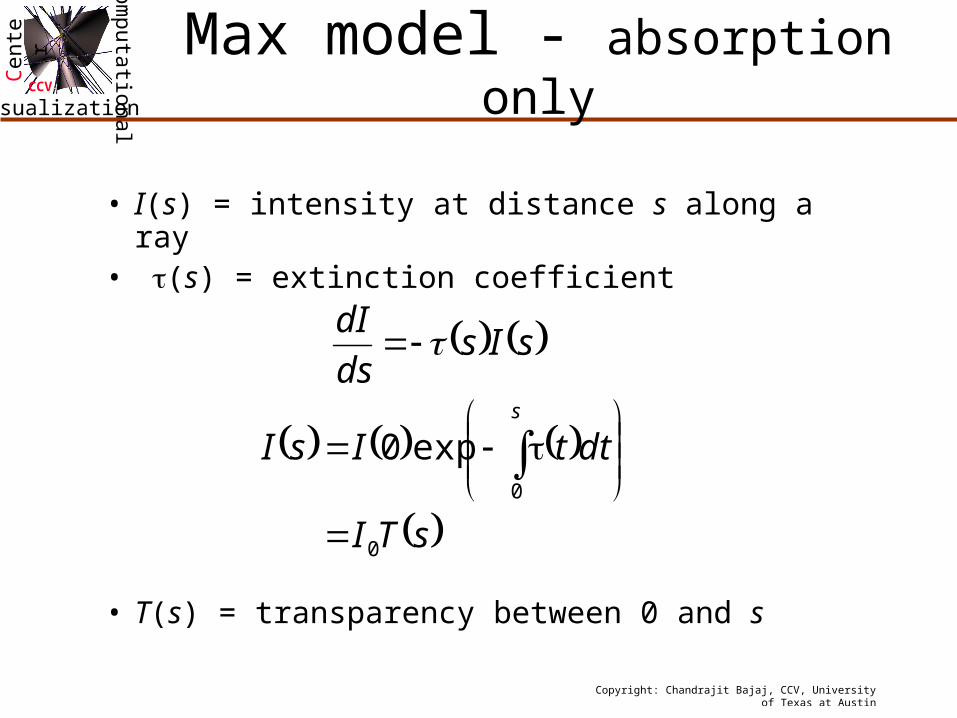
CCVMax model - absorption only
• I(s) = intensity at distance s along a ray• (s) = extinction coefficient
• T(s) = transparency between 0 and s
sIsds
dI
sTI
dttIsIs
0
0
exp0
Copyright: Chandrajit Bajaj, CCV, University of Texas at Austin
ComputationalVisualization
Cent
er
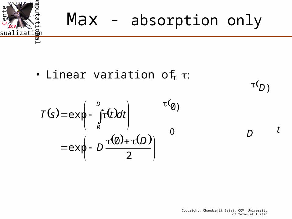
CCVMax - absorption only
• Linear variation of
2
0exp
exp0
DD
dttsTD
t
D
D)
0)
Copyright: Chandrajit Bajaj, CCV, University of Texas at Austin
ComputationalVisualization
Cent
er
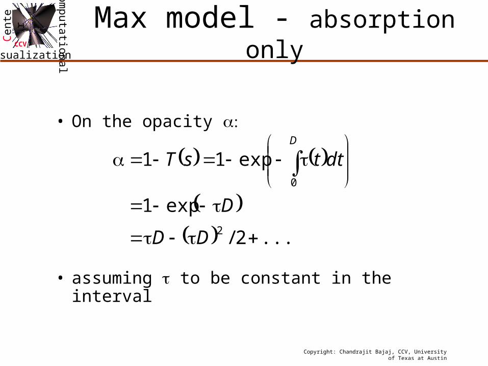
CCVMax model - absorption only
• On the opacity
• assuming to be constant in the interval
...2/
exp1
exp11
2
0
DD
D
dttsTD
Copyright: Chandrajit Bajaj, CCV, University of Texas at Austin
ComputationalVisualization
Cent
er
CCV
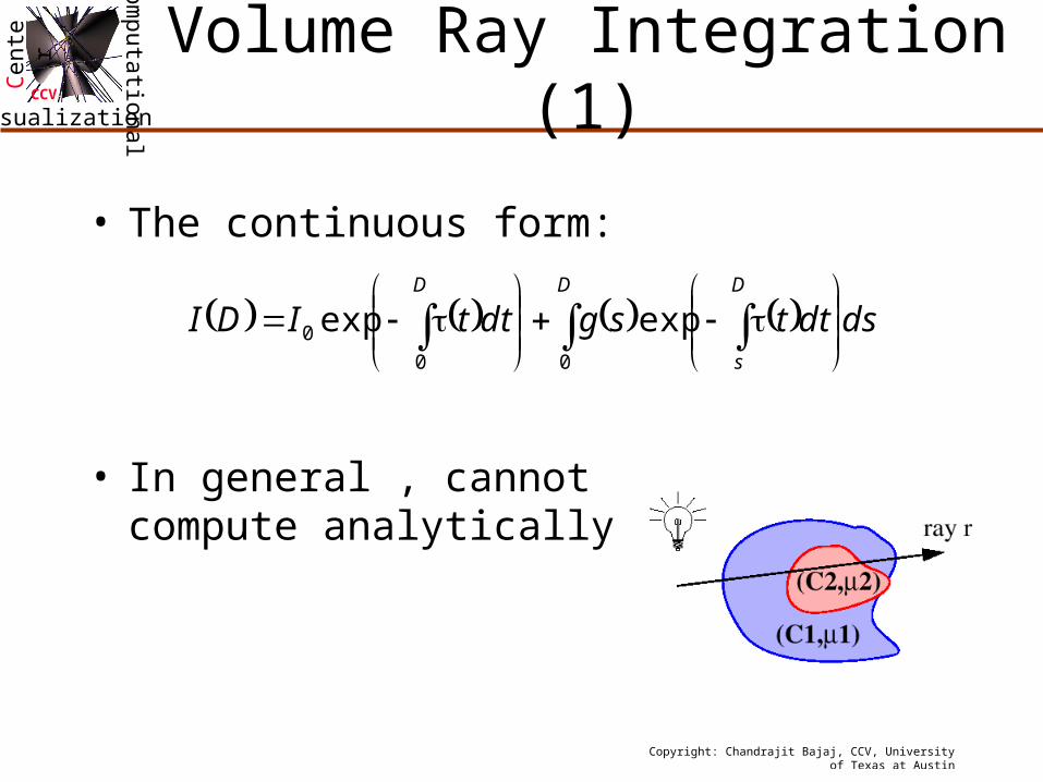
• The continuous form:
• In general , cannot compute analytically
dsdttsgdttIDID D
s
D
00
0 expexp
Volume Ray Integration (1)
Copyright: Chandrajit Bajaj, CCV, University of Texas at Austin
ComputationalVisualization
Cent
er
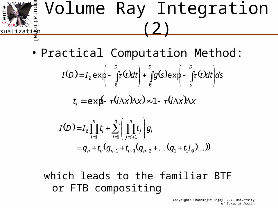
CCVVolume Ray Integration (2)
• Practical Computation Method:
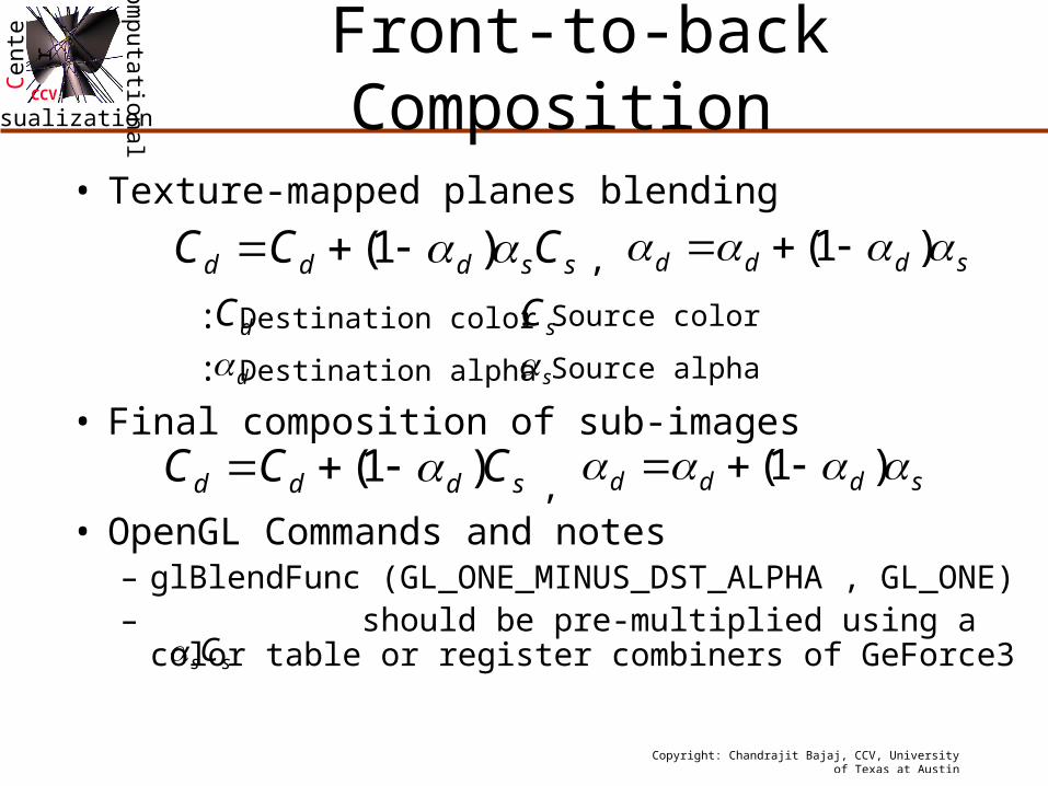
which leads to the familiar BTF or FTB compositing
dsdttsgdttIDID D
s
D
00
0 expexp
xxixxiti 1exp
011211
1 110
Itggtgtg
gttIDI
nnnnn
n
ii
n
ijj
n
ii
Copyright: Chandrajit Bajaj, CCV, University of Texas at Austin
ComputationalVisualization
Cent
er
CCVg(s)
• g(s) could be:– Self-emitting particle glow– Reflected color, obtained via illumination
• The color is usually the sum of emitted color E and reflected color R
Copyright: Chandrajit Bajaj, CCV, University of Texas at Austin
ComputationalVisualization
Cent
er
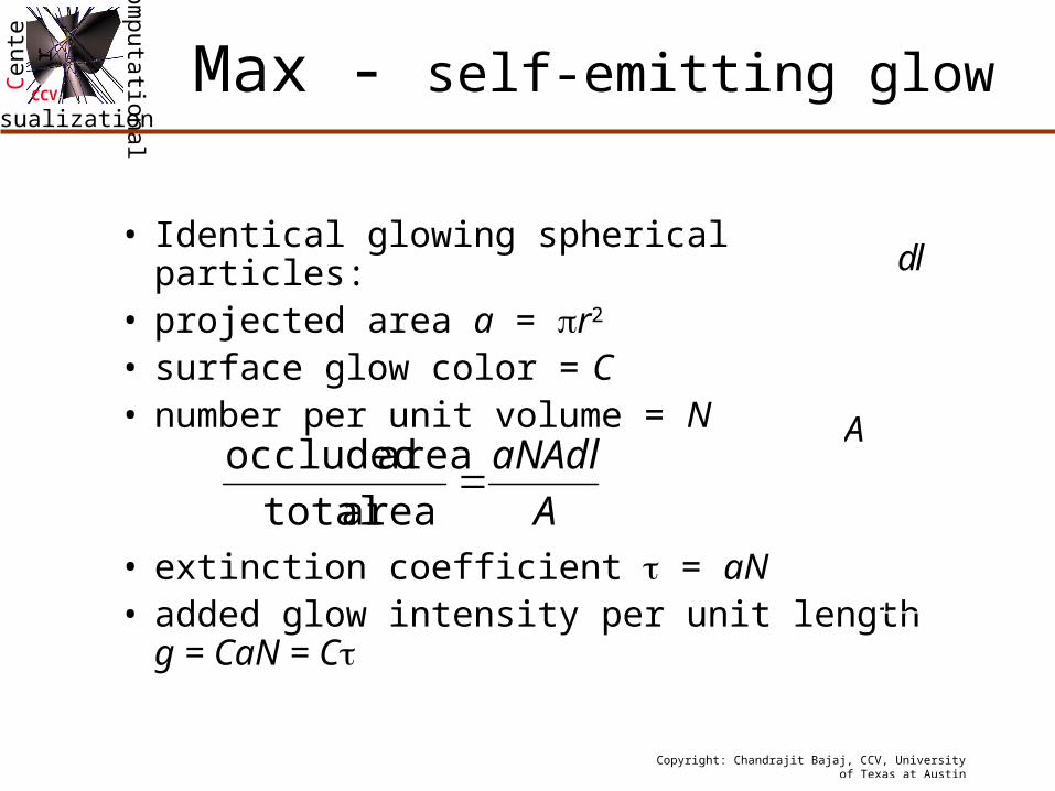
CCVMax - self-emitting glow
• Identical glowing spherical particles:• projected area a = r2
• surface glow color = C• number per unit volume = N
• extinction coefficient = aN• added glow intensity per unit length
g = CaN = C
A
aNAdl
area total
area occluded
dl
A
Copyright: Chandrajit Bajaj, CCV, University of Texas at Austin
ComputationalVisualization
Cent
er
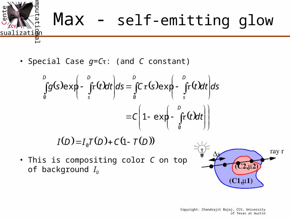
CCVMax - self-emitting glow
• Special Case g=C: (and C constant)
• This is compositing color C on top of background I0
DTCDTIDI 10
D
D D
s
D D
s
dttC
dsdttsCdsdttsg
0
00
exp1
expexp
Copyright: Chandrajit Bajaj, CCV, University of Texas at Austin
ComputationalVisualization
Cent
er
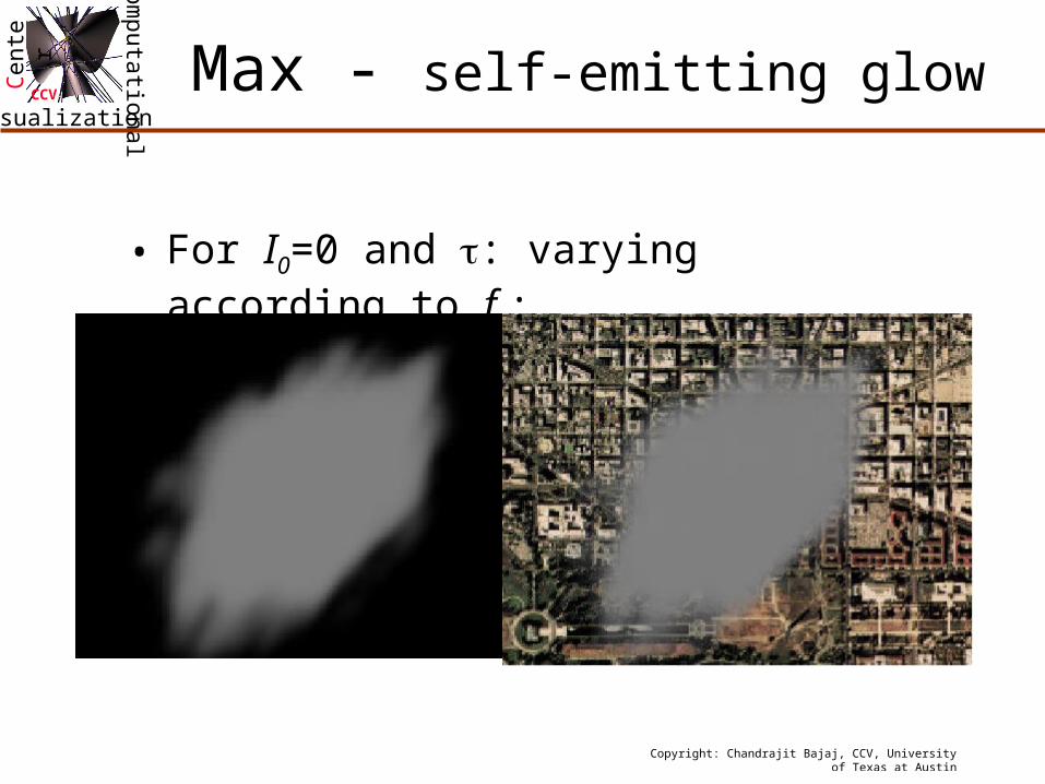
CCVMax - self-emitting glow
• For I0=0 and : varying according to f :
Copyright: Chandrajit Bajaj, CCV, University of Texas at Austin
ComputationalVisualization
Cent
er
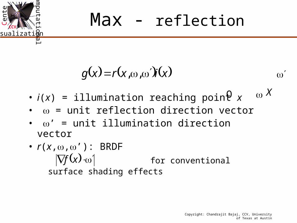
CCVMax - reflection
• i(x) = illumination reaching point x• = unit reflection direction vector• ’ = unit illumination direction vector• r(x,,’): BRDF
for conventional surface shading effects
xixrxg ,,
xf
O
X
Copyright: Chandrajit Bajaj, CCV, University of Texas at Austin
ComputationalVisualization
Cent
er
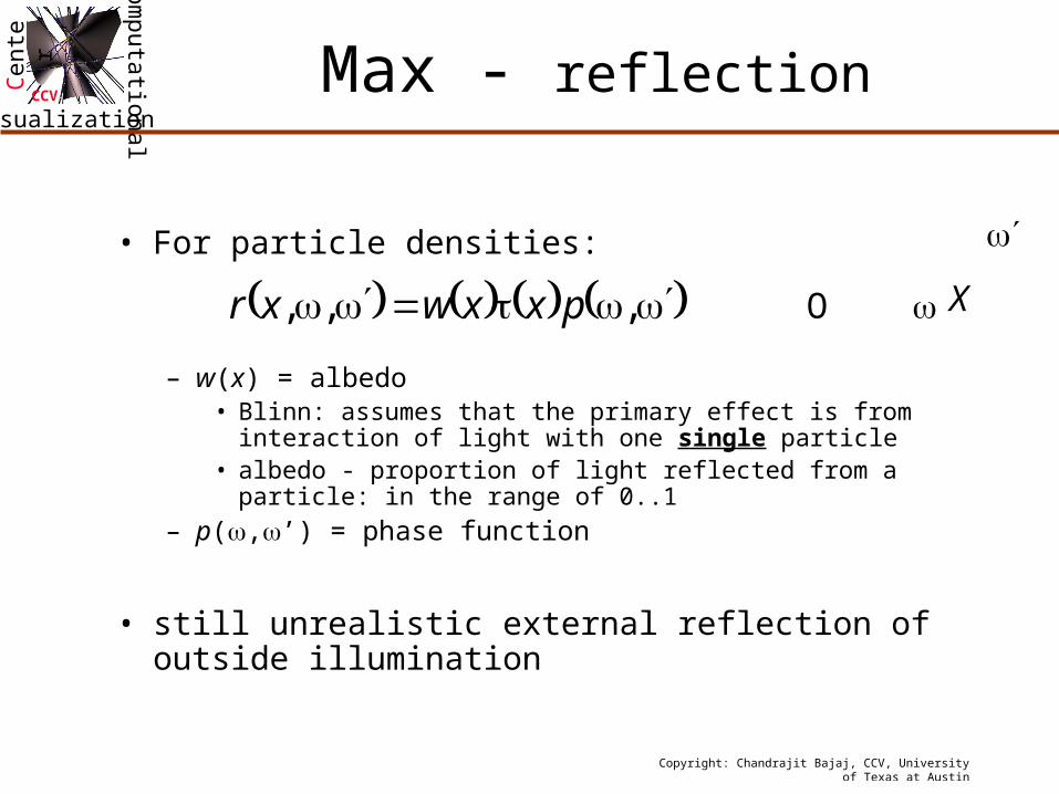
CCVMax - reflection
• For particle densities:
– w(x) = albedo• Blinn: assumes that the primary effect is from interaction
of light with one single particle• albedo - proportion of light reflected from a particle: in the
range of 0..1
– p(,’) = phase function
• still unrealistic external reflection of outside illumination
,,, pxxwxr O
X
Copyright: Chandrajit Bajaj, CCV, University of Texas at Austin
ComputationalVisualization
Cent
er
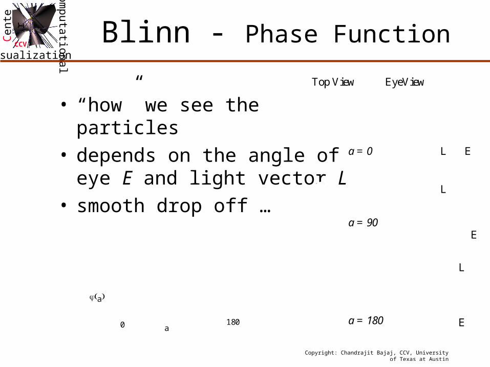
CCVBlinn - Phase Function
• “how” we see theparticles
• depends on the angle ofeye E and light vector L
• smooth drop off …
L E
L
E
L
E
a = 0
a = 90
a = 180
Top View EyeView
a0 180
a
Copyright: Chandrajit Bajaj, CCV, University of Texas at Austin
ComputationalVisualization
Cent
er
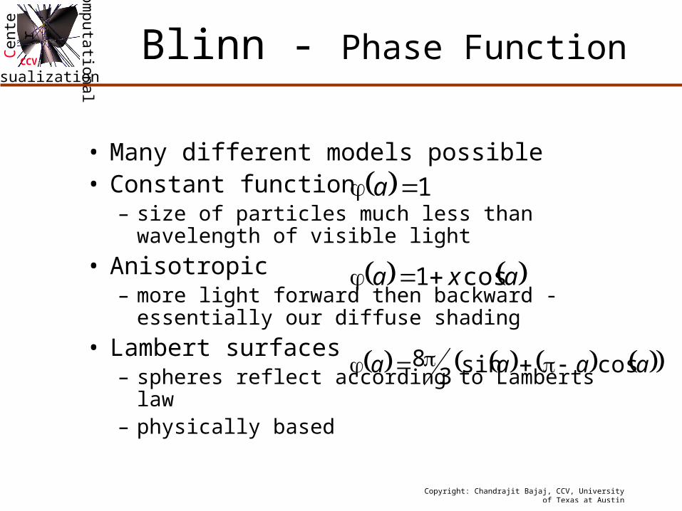
CCVBlinn - Phase Function
• Many different models possible• Constant function
– size of particles much less than wavelength of visible light
• Anisotropic– more light forward then backward - essentially
our diffuse shading
• Lambert surfaces– spheres reflect according to Lamberts law– physically based
1 a
axa cos1
aaaa cossin38
Copyright: Chandrajit Bajaj, CCV, University of Texas at Austin
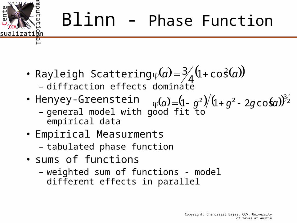
• Henyey-Greenstein– general model with good fit to empirical data
• Empirical Measurments– tabulated phase function
• sums of functions– weighted sum of functions - model different
effects in parallel
aa 2cos143
23
22 cos211 aggga
Copyright: Chandrajit Bajaj, CCV, University of Texas at Austin
ComputationalVisualization
Cent
er
CCVFurther reading
• 3D RGB Image Compression for Interactive Applications,ACM Transactions on Graphics, Vol.20, No.1, pages 10-38, 2001
• Compression-Based 3D Texture Mapping for Real-Time Rendering Graphical Models, Vol. 62, No. 6, pp. 391-410
• Compression-based Ray Casting of Very Large Volume Data in Distributed Environments HPC-Asia 2000, pages 720-725, Beijing, China, May 2000
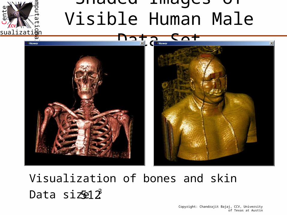
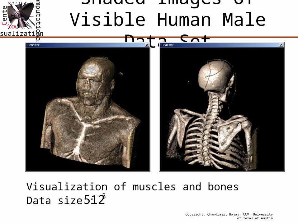
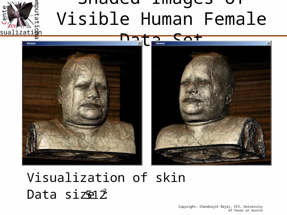
• Parallel Ray Casting of Visible Human on Distributed Memory Architectures Proceedings of Joint EUROGRAPHICS - IEEE TCVG Symposium on Visualization May 26-28, 1999 Vienna, Austria. pp. 269-276
Copyright: Chandrajit Bajaj, CCV, University of Texas at Austin