arX

iv:1

106.

2902

v1 [

phys

ics.

data

-an]

15

Jun

2011

Computational approach to multifractal music

P. Oswiecimkaa, J. Kwapiena, I. Celinskaa,c, S. Drozdza,b, R. Rakb

aInstitute of Nuclear Physics, Polish Academy of Sciences, PL–31-342 Krakow, PolandbFaculty of Mathematics and Natural Sciences, University of Rzeszow, PL–35-959

Rzeszow, PolandcFaculty of Physics and Applied Computer Science, AGH University of Science and

Technology, PL-30-059 Krakow, Poland

Abstract

In this work we perform a fractal analysis of 160 pieces of music belongingto six different genres. We show that the majority of the pieces reveal char-acteristics that allow us to classify them as physical processes called the 1/f(pink) noise. However, this is not true for classical music represented here byFrederic Chopin’s works and for some jazz pieces that are much more corre-lated than the pink noise. We also perform a multifractal (MFDFA) analysisof these music pieces. We show that all the pieces reveal multifractal proper-ties. The richest multifractal structures are observed for pop and rock music.Also the viariably of multifractal features is best visible for popular musicgenres. This can suggest that, from the multifractal perspective, classicaland jazz music is much more uniform than pieces of the most popular genresof music.

Keywords: Fractal, Fractal dimension, Mulifractality, Singularityspectrum.

1. Introduction

Since B. Mandelbrot’s “Fractal Geometry of Nature” was published (Mandeldrot,1982), fractals have an enormous impact on our perception of the surround-ing world. In fact, fractal (i.e. self-similar) structures are ubiquitous innature, and the fractal theory itself contitutes a platform on which variousfields of science, such as biology (Ivanov et al., 1999; Makowiec et al., 2009;

Email address: pawel.oswiecimka@ifj.edu.pl ( P. Oswiecimka)

Preprint submitted to Elsevier May 14, 2018

Rosas et al., 2002), chemistry (Stanley and Meakin, 1988; Udovichenko and Strizhak,2002), physics (Muzy et al., 2008; Oswiecimka, 2006; Subramaniam et al.,2008), and economics (Drozdz et al., 2010; Kwapien et al., 2005; Matia, 2003;Oswiecimka et al., 2005; Zhou, 2009), come across. This (statistical) self-similarity concerns irregularly-shaped empirical structures (Latin word frac-tus means ’rough’) which often elude classical methods of data analysis. Thisinterdisciplinary character of the applied fractal geometry is not confined onlyto science, but also in art, which may be treated as some reflection of real-ity, some interesting fractal features might be discerned. An example of thisare the fractal properties of Jackson Pollock’s paintings (Taylor et al., 1999)and the Zipf’s law describing literary works (Kwapien et al., 2010; Zanette,2006; Zipf, 1949). In a course of time the fractal theory encompassed alsothe multifractal theory dealing with the structures which are convolutionsof different fractals. It turned out that such structures and correspondingprocesses are not rare in nature and the proposed multifractal formalismallowed researchers to introduce distinction between mono- and multifrac-tals (Halsey et al., 1986). Development of those intriguing theories wouldnot have been possible, though, if there had not been substantial progress incomputer science. On the one hand, fractals - due to their structure - caneasily be modelled by using iterative methods, for which the computers areideal tools. On the other hand, however, the multifractal analyses requiresignificant computing power. The result of such an analysis is identificationof diverse patterns in different subsets of data which would be impossiblewithout modern computers. Although relations of mathematics and physicswith music date back to ancient times (Pythagoras of Samos considered musica science of numbers), a new impulse for them arrived together with devel-opments in the fractal methods of time series analysis (Bigerelle and Iost,2000; Ro and Kwon, 2009). The first fractal analysis of music was carriedout in 1970s by Voss and Clarke (Voss and Clarke, 1975), who showed thatthe frequency characteristics of investigated signals behave similar to 1/fnoise. Interestingly, this type of noise (called pink noise or scaling noise)occurs very often in nature (Bak et al., 1987). The 1/f spectral density is anattribute, among others, of meteorological data series, electronic noise occursin almost all electronic devices, statistics of DNA sequences and heart beatrthythm (Bak, 1996). Thus, from this point of view, music imitates naturalprocesses. A note worth making here is that, according to the authors of theabove-cited article, the most pleasent to ear kind of music is just the pinknoise. In 1990s Hsu and Hsu showed that for some classical pieces of Bach

2

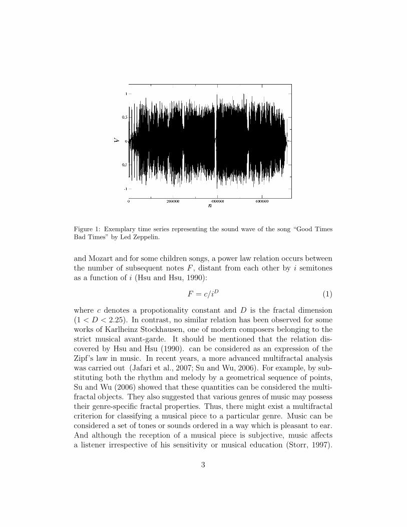
Figure 1: Exemplary time series representing the sound wave of the song “Good TimesBad Times” by Led Zeppelin.

and Mozart and for some children songs, a power law relation occurs betweenthe number of subsequent notes F , distant from each other by i semitonesas a function of i (Hsu and Hsu, 1990):

F = c/iD (1)

where c denotes a propotionality constant and D is the fractal dimension(1 < D < 2.25). In contrast, no similar relation has been observed for someworks of Karlheinz Stockhausen, one of modern composers belonging to thestrict musical avant-garde. It should be mentioned that the relation dis-covered by Hsu and Hsu (1990). can be considered as an expression of theZipf’s law in music. In recent years, a more advanced multifractal analysiswas carried out (Jafari et al., 2007; Su and Wu, 2006). For example, by sub-stituting both the rhythm and melody by a geometrical sequence of points,Su and Wu (2006) showed that these quantities can be considered the multi-fractal objects. They also suggested that various genres of music may possesstheir genre-specific fractal properties. Thus, there might exist a multifractalcriterion for classifying a musical piece to a particular genre. Music can beconsidered a set of tones or sounds ordered in a way which is pleasant to ear.And although the reception of a musical piece is subjective, music affectsa listener irrespective of his sensitivity or musical education (Storr, 1997).

3

Figure 2: Exemplary power spectra (in log-log scale) for six pieces of music representingsix genres (from top to bottom: classical music, jazz, pop music, electronic music, rock,and hard rock). Power-law trends in each panel are indicated by dashed lines, whose slopescorrespond to the corresponding values of β.

4

Therefore, a hypothesis which arises in this context is that music as an objectmay refer not only to the structure of a musical piece but also to the way itis perceived.

2. Power spectral analysis

In our work we analyzed 160 pieces of music from six popular genres:classical music, pop music, rock, hard rock, jazz, and electronic music. Thefirst one, classical music, was represented by 38 works by Frederick Chopin,divided into three periods of his career. Pop music consisted of 51 songs per-formed by Britney Spears, rock and hard rock music - 20 songs performed byLed Zeppelin and 20 songs by Steve Vai, respectively, jazz - 25 compositionsperformed by Miles Davies or Glenn Miller. Finally, an electronic music con-sisted of 6 pieces of music by Royskopp. All the analyzed pieces were writtenin the WAV format. In this format the varying amplitude of a sound waveV (t) is encoded by a 16-bit stream sampled with 44,1 kHz frequency. Afterencoding, the amplitude V (t) was expressed by a time series of length depend-ing on the temporal length of a given piece of music (several million points,on average). An exemplary time series encoding a randomly selected songis displayed in Figure 1. We started our analysis with calculating the powerspectrum S(f) for each piece of music. This quantity carries informationon power density of sound wave components of frequency (f ; df). Accordingto the Wiener-Khinchin theorem, S(f) is equal to the Fourier transform ofautocorrelation function or, equivalently, the squared modulus of a signal’sFourier transform:

S(f) = |X(f)|2 (2)

where

X(f) =

∞∫

−∞

x(t)e−2πiftdt (3)

is the Fourier transform of a signal x(t). If the power spectrum decreaseswith f as 1/fβ, (β ≥ 0), it means that the signal under study is characterizedby log-range autocorrelation within the scales described by the correspond-ing frequencies f . The faster is the decrease of S(f) (i.e. the higher valueof β), the stronger is the autocorrelation of the signal. It is worth recallinghere that the Brownian motion corresponds to β = 2, while the white noise(uncorrelated signal) to β = 0. Since the exponent β can easily be trans-formed into the Hurst exponent (a well-known notion in fractal analysis) or

5

Figure 3: Exponent β calculated for each piece of music analyzed in the present work(short horizontal lines). Columns correspond to individual artists, periods of their career(Chopin), or albums. Dotted vertical lines separate different music genres.

into the fractal dimension, the power spectrum can be classified among themonofractal techniques of data analysis. The power spectra were calculatedfor each piece of music. In most cases, the graph S(f) was a power-law de-creasing function for frequencies 0.1-10 kHz with the slope characteristic fora given piece. The notable exceptions were works of Chopin for which thegraphs were scaling between 1 and 10 kHz. Six representative spectra fordifferent genres are shown in Figure 2. To each empirical spectrum S(f) apower function was fitted (the straight lines in Figure 2 ) within the observedcorresponding power-law regime. A slope of the fitted function correspondsto the exponent β. All the calculated values of β, are exhibited in Figure3. As it can be seen, the highest values of β correspond to works of F.Chopin (classical music,βMAX = 4.4) and some works of Glenn Miller (jazz,βMAX = 4.8). Exponents in these cases are much higher than 2 whichmeans that the underlying processes are more correlated than the Brownianmotion. Also several songs by Led Zeppelin (rock) have β > 2 but not soprominent as the pieces from those genres mentioned before. Interestingly,β for Led Zeppelin declines with time. For their chronologically first album,the highest exponent is 2.8, while for the subsequent albums it drops to 2.3and 2.1, respectively. For the other analyzed music genres, i.e. electronic,pop, rock and hard rock music, 1 < β < 2. It is also worth mentioning that

6

for several jazz pieces, the exponent β drops below 1, which means that theyapproach white noise. An author of these songs is Miles Davies, one of themost significant jazz artists, who often was a precursor of new styles andsounds. To summarize this part of our analysis, we can say that from thepower spectrum perspective, the majority of the analyzed pieces of music canin fact be considered the 1/f processes. This is even more evident for morepopular music genres like pop and rock than for rather exclusive genres likejazz and classical music.

3. Multifractal analysis of musical compositions

In order to have a deeper insight into dynamics of the investigated sig-nals we performed also multifractal analysis of data. We used one of themost popular and reliable methods - the Multifractal Detrended FluctuationAnalysis (MFDFA) (Kantelhardt, 2002). This method allows us to calcu-late fractal dimensions and Hoelder exponents for individual components ofa signal decomposed with respect to the size of fluctuations. Consecutivesteps of this procedure are presented below. At the beginning we calculatethe so-called profile, which is the cumulative sum of the analyzed signal:

Y (i) =

i∑

j=1

[xj − 〈x〉] for i = 1, 2, ...N, (4)

where 〈x〉 donotes the signal’s mean, and N denotes its length. The sub-traction of the mean value is not necessary, because a trend is eliminated inthe next steps. Then we divide the profile Y (i) into Ns disjoint segments oflentgh s (Ns = N/s). In order to take into account all the points (at theend of the signal’s profile some data can be neglected), the dividing proce-dure has to be repeated starting from the end of Y (i). In consequence, weobtain 2Ns segments. In each segment ν, the estimated trend is subtractedfrom the data. The trend is represented by a polynomial P l

ν of order l. Thepolynomial’s order used in calculation determines the variant of the method.Thus, for l = 1 we have MFDFA1, for l = 2 - MFDFA2, and so on. Afterdetrending the data, its variance has to be calculated in each segment:

F 2(s, ν) =1

s

s∑

i=1

{Y [(ν − 1)s + i] − P lν(i)}2 for ν = 1, 2, ...Ns (5)

7

Figure 4: Exemplary fluctuation function Fq (in log − log scale) for six pieces of musicrepresenting six genres (from top to bottom: classical music, jazz, pop music, electronicmusic, rock and hard rock). Each line represents Fq calculated for particular q values inthe range from -4 to 4

8

or

F 2(s, ν) =1

s

s∑

i=1

{Y [N−(ν−Ns)s+i]−P lν(i)}2 for ν = Ns+1, Ns+2, ...2Ns

(6)The variances are then averaged over all the segments and, finally, one getsthe qth order fluctuation function given by:

Fq(s) =

{

1

2Ns

2Ns∑

ν=1

[F 2(s, ν)]q/2

}1/q

, (7)

where the exponent q belongs to R \ {0}. This procedure has to be repeatedfor different values of s. If the analyzed signal has any fractal properties, thefluctuation function behaves as:

Fq(s) ∼ sh(q), (8)

where h(q) denotes the generalized Hurst exponents. A constant h(q) for allq’s means that the studied signal is monofractal and h(q) = H (the ordinaryHurst exponent). For multifractal signals, h(q) is a monotonically decreasingfunction of q. It can be easily noticed that, by varying the q parameter,it is possible to decompose the time series into fluctuation components ofdifferent character: for q > 0 the fluctuation function mostly describes largefluctuations, whereas for q < 0 the main contribution to the Fq comes fromsmall fluctuations. By knowing the h(q) spectrum for a given set of data, wecan calculate its singularity (multifractal) spectrum:

α = h(q) + qh′

(q) and f(α) = q[α− h(q)] + 1, (9)

where h′

(q) stands for the derivative of h(q) with respect to q, the Hoelderexponent α donotes singularity strength, and f(α) is the fractal dimensionof the set of points characterized by α. For a monofractal time series, thesingularity spectrum reduces to a single point (H, 1), while for multifractaltime series, the spectrum assumes the shape of an inverted parabola. Themultifractal strength is a quantity which describes the richness of multifrac-tality, i.e., how diverse are values of the Hoelder exponents in a data set. Itcan be estimated by the width of the f(α) parabola:

∆α = αmax − αmin (10)

9

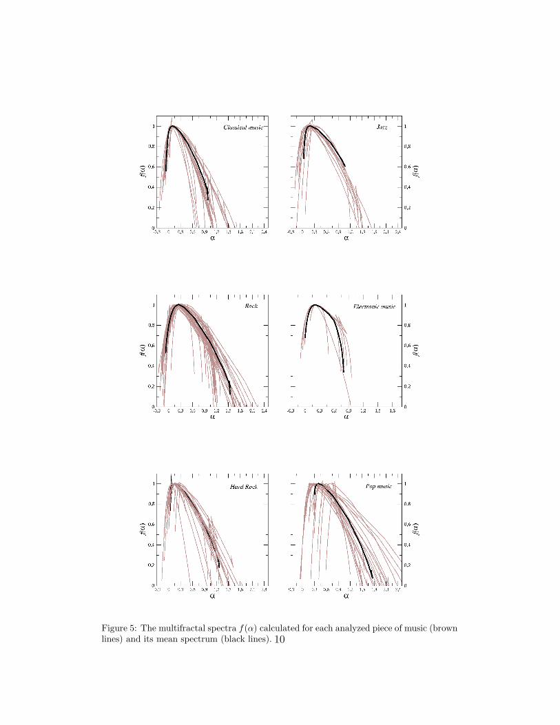
Figure 5: The multifractal spectra f(α) calculated for each analyzed piece of music (brownlines) and its mean spectrum (black lines). 10

where αmin and αmax stand for the extreme values of α. The bigger is α thericher is the multifractal.Using MFDFA2, which guarantees stability of results, we calculated the fluc-tuation function Fq for all the analyzed signals in the scale s range from 50to 100,000 points. The value of q was increased by 0.2 in the range from-4 to 4. Exemplary fluctuation functions for our six music genres are shownin Figure 4. All the calculated Fq functions are characterized by a powerlaw dependence on the scale for all q’s. However, the range of scaling variesslightly for different pieces. By looking at the shown examples, it is easyto notice that for F. Chopin, Britney Spears, Glenn Miller, and Steve Vai,the scaling involves almost all the considered values of s, while for electronicmusic we can distinguish two scaling ranges: the longer one for the scales40 < s < 10, 000 and the shorter one for 10, 000 < s < 100, 000. Such doublescaling appears also occasionally for the other genres of music. However, forthe most cases, we observe only one type of scaling. In Figure 4 we can alsonotice a clear dependence of the h(q) exponent (the slope coefficient of Fq indouble log scale) on q. And so, the largest values of h(q) correspond to q < 0,whereas for q > 0, h(q) takes smaller values. Therefore already at this stageof calculations, it can be seen that the analyzed signals can have distinct mul-tifractal properties. It is also worth to mention that for the large scales (e.g.for jazz s > 40, 000, for hard rock s > 20, 000), scaling loses its multifractaltraits, and h(q) does not depend on q. It is related to the limited rangeof nonlinear correlations (Drozdz et al., 2009). The scale s, for which thescaling character of Fq changes, sets a limit for estimation of the multifrac-tal spectrum. For all the fluctuation functions, we estimated the singularityspectra f(α). Figure 5 presents the multifractal spectra (grey lines) and thecorresponding mean multifractal spectra (black lines) for the music genres towhich the given pieces belong. All the mean spectra are asymmetric. Theright part which describe the small amplitude fluctuations is clearly longer.This effect is best visible for the rock, hard rock, and pop songs. Locationsof the extrema of these spectra (α ≈ 0.2) suggest considerably antipersistentbehavior of the analyzed time series. We can easily see that the width of themultifractal spectra for a particular genre fluctuates considerably. Nevertheless, all the spectra are characterized by the widths large enough that theycan be regarded as multifractal structures. This confirms observation madeabove for the Fq function. The narrowest mean multifractal spectrum wasobserved for electronic music (∆α = 0.85). Classical music and jazz displaymutually comparable widths of, respectively, 1.0 and 1.1. The widest mean

11

Figure 6: Value of ∆α calculated for each analyzed piece of music (short horizontal lines).Columns correspond to individual artist, periods of their career, or albums. Dotted verticallines separate different genres of music.

f(α) is seen for hard rock (1.22), rock (1.5), and pop (1.8). Thus, from thispoint of view, the richest multifractal (the richest dynamics of processes) isan attribute of the most popular music genres. The more exclusive genres arecharacterized by poorer multifractals. Figure 6 presents a collection of all thecalculated widths of f(α). Vertical lines separate different music genres andeach piece is represented by a single horizontal line. As it can be seen, themost variable multifractal spectra widths characterize pop (0.5 < α < 2.8),rock (0.5 < α < 2.1) and hard rock (0.51 < α < 2.15) music. Thus, onaccount of multifractal properties, the pieces belonging to these genres differmarkedly among themselves. Much more consistent from this point of vieware the pieces of classical music, jazz and electronic music. We can drawtherefore a conclusion that this is the richness of multifractal forms whatdistinguishes popular music from the more exclusive and the less listened tomusical genres.

4. Conclusions

To sum up, our work presents results of a fractal analysis of selected musicworks belonging to six different genres: pop, rock, hard rock, jazz, classical,and electronic music. The results confirm that the amplitude signals V (t)

12

are characterized by the power spectrum falling off according to a power law:S(f) ∼ 1/fβ. Interestingly, rate of this fall can be characteristic for a par-ticular genre. For classical music and some pieces of jazz, S(f) declines thefastest, while for popular music (pop, rock, hard rock , and electronic mu-sic ) the power spectrum falls more slowly suggesting less correlated signals.The same signals were also subject to a multifractal analysis. It turned outthat such data demonstrate well-developed multifractality. Interestingly, themost variable widths of multifractal spectra (and also the widest singularityspectra thus strongest nonlinear correlations) were observed for popular gen-res like pop and rock. For the remaining genres, the multifractal propertieswere rather similar among the pieces. Therefore, from this point of view, thepopular music is characterized by the amplitude signals with different degreeof correlations, whereas more sophisticated musical genres (classical, jazz)are more consistent in this matter.

References

Bak, P., Tang, C., Wiesenfield, K., 1987. Self-organized criticality: an expla-nation of 1 /f noise. Phys. Rev. Lett. 59, 381-384.

Bak, P., 1996. How Nature Works: The Science of Self-Organised Criticality,Copernicus.

Bigerelle, M., Iost, A., 2000. Fractal dimension and classification of music.Chaos, Solitons & Fractals 11, 2179-2192.

Drozdz, S., Kwapien, J., Oswiecimka, P., Rak, R., 2009. Quantitative featuresof multifractal subtleties in time series. EPL 88, 60003.

Drozdz, S., Kwapien, J., Oswiecimka, P., Rak, R., 2010. The foreign ex-change market: return distributions, multifractality, anomalous multifrac-tality and the Epps effect. New J. Phys. 12 105003.

Halsey, T.C., Jensen, M.H., Kadanoff, L.P., Procaccia, I., Shraiman, B.I.,1986. Fractal measures and their singularities: The characterization ofstrange sets. Phys. Rev. A 33 1141.

Hsu, K.J., Hsu, A.J., 1990. Fractal geometry of music. Proc. Natl. Acad. Sci.USA 87 938-341.

13

Ivanov, P.Ch., Amaral,A.N., Goldberger, A.L., Havlin, Sh., Rosenblum,M.G., Struzik Z.R. and Stanley, H.E., 1999. Multifractality in humanheartbeat dynamics. Nature 399, 461-465.

Jafari, G.R., Pedram, P., and Hedayatifar, L., 2007. Long-range correlationand multifractality in Bach’s Inventions pitches. J. Stat. Mech., P04012.

Kantelhardt, J.W., Zschiegner, S.A., Koscielny-Bunde, E., Bunde, A.,Havlin, Sh., and Stanley, H.E., 2002. Multifractal detrended fluctuationanalysis of nonstationary time series. Physica A 316, 87-114.

Kwapien, J., Oswiecimka, P., Drozdz, S., 2005. Components of multifractalityin high-frequency stock returns. Physica A 350, 466-474 .

Kwapien, J., Drozdz, S., Orczyk, A., 2010. Linguistic complexity: english vs.polish, text vs. corpus. Acta Phys, Pol. A 117, 716.

Makowiec, D., Dudkowska, A., Ga laska, R., Rynkiewicz, A., 2009. Multi-fractal estimates of monofractality in RR-heart series in power spectrumranges. Physica A 388 3486-3502.

Mandelbrot, B.B., 1982. The Fractal Geometry of Nature, W.H. Freemanand Company, New York.

Matia, K., Ashkenazy, Y., Stanley, H.E., 2003. Multifractal Properties ofPrice Fluctuations of Stocks and Commodities. EPL 61, 422-428.

Muzy, J.F., Bacry, E., Baile, R., and Poggi, P., 2008. Uncovering latentsingularities from multifractal scaling laws in mixed asymptotic regime.Application to turbulence. EPL 82, 60007.

Oswiecimka, P., Kwapien, J., Drozdz, S., 2005. Multifractality in the stockmarket: price increments versus waiting times. Physica A 347, 626-638.

Oswiecimka, P., Kwapien, J., Drozdz, S., 2009. Wavelet versus DetrendedFluctuation Analysis of multifractal structures. Phys. Rev. E 74,016103.

Ro, W., Kwon, Y., 2009. 1/f Noise analysis of songs in various genre of music.Chaos, Solitons & Fractals 42, 2305-2311.

Rosas, A., Nogueira, E.Jr., Fontanari, J.F., 2002. Multifractal analysis ofDNA walks and trails. Phys. Rev. E 66, 061906.

14

Stanley, H.E. and Meakin, P., 1988. Multifractal phenomena in physics andchemistry. Nature 335, 405-409.

Storr, A., 1997. Music and the Mind. HarperCollinsPublisher, London.

Su, Z.-Y., Wu, T., 2006. Multifractal analyses of music sequences. Physica D221 188-194.

Subramaniam, A.R., Gruzberg, L.A., Ludwig, A.W.W., 2008. Boundary crit-icality and multifractality at the two-dimensional spin quantum Hall tran-sition. Phys. Rev. B 78, 245105.

Taylor, R.P., Micolich, A.P., Jonas, D., 1999. Fractal analysis of Pollock’sdrip paintings. Nature 399, 422.

Udovichenko, V.V., and Strizhak, P.E., 2002. Multifractal Properties of Cop-per Sulfide Film Formed in Self-Organizing Chemical System. Theoreticaland Experimental Chemistry 38, 259-262.

Voss, R.F., Clarke, J., 1975. 1/f noise in music and speech. Nature 258 317-318.

Zanette, D., H., 2006. Zipf’s law and the creation of musical context. MusicaeScientiae 10, 3-18.

Zhou, W.-X., 2009. The components of empirical multifractality in financialreturns. EPL 88, 28004.

Zipf, G.K., 1949. Human behavior and the principle of least effort. Addison-Wesley.

15