Computations with p-adic numbers Xavier Caruso January 23, 2017 Abstract This document contains the notes of a lecture I gave at the “Journ´ ees Nationales du Calcul Formel 1 ” (JNCF) on January 2017. The aim of the lecture was to discuss low-level algorithmics for p-adic numbers. It is divided into two main parts: first, we present various implementations of p-adic numbers and compare them and second, we introduce a general framework for studying precision issues and apply it in several concrete situations. Contents 1 Introduction to p-adic numbers 3 1.1 Definition and first properties ............................. 3 1.2 Newton iteration over the p-adic numbers ...................... 9 1.3 Similarities with formal and Laurent series ...................... 12 1.4 Why should we implement p-adic numbers? ..................... 15 2 Several implementations of p-adic numbers 19 2.1 Zealous arithmetic ................................... 19 2.2 Lazy and relaxed arithmetic .............................. 23 2.3 Floating-point arithmetic ................................ 31 2.4 Comparison between paradigms ............................ 34 3 The art of tracking p-adic precision 42 3.1 Foundations of the theory of p-adic precision ..................... 42 3.2 Optimal precision and stability of algorithms ..................... 53 3.3 Lattice-based methods for tracking precision ..................... 70 References 81 Introduction The field of p-adic numbers, Q p , was first introduced by Kurt Hensel at the end of the 19th century in a short paper written in German [36]. From that time, the popularity of p-adic numbers has grown without interruption throughout the 20th century. Their first success was materialized by the famous Hasse–Minkowski’s Theorem [75] that states that a Diophantine equation of the form P (x 1 ,...,x n )=0 where P is a polynomial of total degree at most 2 has a solution over Q if and only if it has a solution over R and a solution over Q p for all prime numbers p. This characterization is quite interesting because testing whether a polynomial equation has a p-adic solution can be carried out in a very efficient way using analytic methods just like over the reals. This kind of strategy is nowadays ubiquitous in many areas of Number Theory and Arithmetic 1 (French) National Computer Algebra Days 1
Transcript
Computations with p-adic numbers
Xavier Caruso
January 23, 2017
Abstract
This document contains the notes of a lecture I gave at the “Journees Nationales duCalcul Formel1” (JNCF) on January 2017. The aim of the lecture was to discuss low-levelalgorithmics for p-adic numbers. It is divided into two main parts: first, we present variousimplementations of p-adic numbers and compare them and second, we introduce a generalframework for studying precision issues and apply it in several concrete situations.
3 The art of tracking p-adic precision 423.1 Foundations of the theory of p-adic precision . . . . . . . . . . . . . . . . . . . . . 423.2 Optimal precision and stability of algorithms . . . . . . . . . . . . . . . . . . . . . 533.3 Lattice-based methods for tracking precision . . . . . . . . . . . . . . . . . . . . . 70
References 81
Introduction
The field of p-adic numbers, Qp, was first introduced by Kurt Hensel at the end of the 19th centuryin a short paper written in German [36]. From that time, the popularity of p-adic numbers hasgrown without interruption throughout the 20th century. Their first success was materializedby the famous Hasse–Minkowski’s Theorem [75] that states that a Diophantine equation of theform P (x1, . . . , xn) = 0 where P is a polynomial of total degree at most 2 has a solution overQ if and only if it has a solution over R and a solution over Qp for all prime numbers p. Thischaracterization is quite interesting because testing whether a polynomial equation has a p-adicsolution can be carried out in a very efficient way using analytic methods just like over the reals.This kind of strategy is nowadays ubiquitous in many areas of Number Theory and Arithmetic
1(French) National Computer Algebra Days
1
Geometry. After Diophantine equations, other typical examples come from the study of numberfields: we hope deriving interesting information about a number field K by studying carefullyall its p-adic incarnations K ⊗Q Qp. The ramification of K, its Galois properties, etc. can be —and are very often — studied in this manner [69, 65]. The class field theory, which providesa precise description of all Abelian extensions2 of a given number field, is also formulated inthis language [66]. The importance of p-adic numbers is so prominent today that there is stillnowadays very active research on theories which are dedicated to purely p-adic objects: one canmention for instance the study of p-adic geometry and p-adic cohomologies [6, 58], the theory ofp-adic differential equations [50], Coleman’s theory of p-adic integration [24], the p-adic Hodgetheory [14], the p-adic Langlands correspondence [5], the study of p-adic modular forms [34],p-adic ζ-functions [52] and L-functions [22], etc. The proof of Fermat’s last Theorem by Wilesand Taylor [81, 78] is stamped with many of these ideas and developments.
Over the last decades, p-adic methods have taken some importance in Symbolic Computationas well. For a long time, p-adic methods have been used for factoring polynomials over Q [56].More recently, there has been a wide diversification of the use of p-adic numbers for effectivecomputations: Bostan et al. [13] used Newton sums for polynomials over Zp to compute composedproducts for polynomials over Fp; Gaudry et al. [32] used p-adic lifting methods to generategenus 2 CM hyperelliptic curves; Kedlaya [49], Lauder [54] and many followers used p-adiccohomology to count points on hyperelliptic curves over finite fields; Lercier and Sirvent [57]computed isogenies between elliptic curves over finite fields using p-adic differential equations.
The need to build solid foundations to the algorithmics of p-adic numbers has then emerged.This is however not straightforward because a single p-adic number encompasses an infiniteamount of information (the infinite sequence of its digits) and then necessarily needs to betruncated in order to fit in the memory of a computer. From this point of view, p-adic numbersbehave very similarly to real numbers and the questions that emerge when we are trying toimplement p-adic numbers are often the same as the questions arising when dealing with roundingerrors in the real setting [62, 26, 63]. The algorithmic study of p-adic numbers is then locatedat the frontier between Symbolic Computation and Numerical Analysis and imports ideas andresults coming from both of these domains.
Content and organization of this course. This course focuses on the low-level implementation ofp-adic numbers (and then voluntarily omits high-level algorithms making use of p-adic numbers)and pursues two main objectives. The first one is to introduce and discuss the most standardstrategies for implementing p-adic numbers on computers. We shall detail three of them, each ofthem having its own spirit: (1) the zealous arithmetic which is inspired by interval arithmeticin the real setting, (2) the lazy arithmetic with its relaxed improvement and (3) the p-adicfloating-point arithmetic, the last two being inspired by the eponym approaches in the real setting.
The second aim of this course is to develop a general theory giving quite powerful tools tostudy the propagation of accuracy in the p-adic world. The basic underlying idea is to linearizethe situation (and then model the propagation of accuracy using differentials); it is once againinspired from classical methods in the real case. However, it turns out that the non-archimedeannature of Qp (i.e. the fact that Z is bounded in Qp) is the source of many simplifications whichwill allow us to state much more accurate results and to go much further in the p-adic setting.As an example, we shall see that the theory of p-adic precision yields a general strategy forincreasing the numerical stability of any given algorithm (assuming that the problem it solves iswell-conditioned).
This course is organized as follows. §1 is devoted to the introduction of p-adic numbers:we define them, prove their main properties and discuss in more details their place in NumberTheory, Arithmetic Geometry and Symbolic Computation. The presentation of the standardimplementations of p-adic numbers mentioned above is achieved in §2. A careful comparison
2An abelian extension is a Galois extension whose Galois group is abelian.
2
between them is moreover proposed and supported by many examples coming from linear algebraand commutative algebra. Finally, in §3, we expose the aforementioned theory of p-adic precision.We then detail its applications: we will notably examine many very concrete situations and, foreach of them, we will explain how the theory of p-adic precision helps us either in quantifying thequalities of a given algorithm regarding to numerical stability or, even better, in improving them.
Acknowledgments. This document contains the (augmented) notes of a lecture I gave at the“Journees Nationales du Calcul Formel3” (JNCF) on January 2017. I heartily thank the organizersand the scientific committee of the JNCF for giving me the opportunity to give these lecturesand for encouraging me to write down these notes. I am very grateful to Delphine Boucher,Nicolas Brisebarre, Claude-Pierre Jeannerod, Marc Mezzarobba and Tristan Vaccon for theircareful reading and their helpful comments on an earlier version of these notes.
Notation. We use standard notation for the set of numbers: N is the set of natural integers(including 0), Z is the set of relative integers, Q is the set of rational numbers and R is the setof real numbers. We will sometimes use the soft-O notation O(−) for writing complexities; werecall that, given a sequence of positive real numbers (un), O(un) is defined as the union of thesets O(un logk un) for k varying in N.
Throughout this course, the letter p always refers to a fixed prime number.
1 Introduction to p-adic numbers
In this first section, we define p-adic numbers, discuss their basic properties and try to explain,by selecting a few relevant examples, their place in Number Theory, Algebraic Geometry andSymbolic Computation. The presentation below is voluntarily very summarized; we refer theinterested reader to [2, 35] for a more complete exposition of the theory of p-adic numbers.
1.1 Definition and first properties
p-adic numbers are very ambivalent objects which can be thought of under many different angles:computational, algebraic, analytic. It turns out that each point of view leads to its own definitionof p-adic numbers: computer scientists often prefer viewing a p-adic number as a sequence ofdigits while algebraists prefer speaking of projective limits and analysts are more comfortablewith Banach spaces and completions. Of course all these approaches have their own interestand understanding the intersections between them is often the key behind the most importantadvances.
In this subsection, we briefly survey all the standard definitions of p-adic numbers and provideseveral mental representations in order to try as much as possible to help the reader to develop agood p-adic intuition.
1.1.1 Down-to-earth definition
Recall that each positive integer n can be written in base p, that is as a finite sum:
n = a0 + a1p+ a2p2 + · · ·+ a`p
`
where the ai’s are integers between 0 and p−1, the so-called digits. This writing is moreoverunique assuming that the most significant digit a` does not vanish. A possible strategy to computethe expansion in base p goes as follows. We first compute a0 by noting that it is necessarily theremainder in the Euclidean division of n by p: indeed it is congruent to n modulo p and lies inthe range [0, p−1] by definition. Once a0 is known, we compute n1 = n−a0
quotient in the Euclidean division of n by p. Clearly n1 = a1 + a2p+ · · ·+ a`p`−1 and we can now
compute a1 repeating the same strategy. Figure 1.1 shows a simple execution of this algorithm.By definition, a p-adic integer is an infinite formal sum of the shape:
x = a0 + a1p+ a2p2 + · · ·+ aip
i + · · ·
where the ai’s are integers between 0 and p−1. In other words, a p-adic integer is an integerwritten in base p with an infinite number of digits. We will sometimes alternatively write x asfollows:
x = . . . ai . . . a3a2a1a0p
or simplyx = . . . ai . . . a3a2a1a0
when no confusion can arise. The set of p-adic integers is denoted by Zp. It is endowed with anatural structure of commutative ring. Indeed, we can add, subtract and multiply p-adic integersusing the schoolbook method; note that handling carries is possible since they propagate on theleft. The ring of natural integers N appears naturally as a subring of Zp: it consists of p-adicintegers . . . ai . . . a3a2a1a0 for which ai = 0 when i is large enough. Note in particular that theinteger p writes . . . 0010 in Zp and more generally pn writes . . . 0010 . . . 0 with n ending zeros. Asa consequence, a p-adic integer is a multiple of pn if and only if it ends with (at least) n zeros.Remark that negative integers are p-adic integers as well: the opposite of n is, by definition, theresult of the subtraction 0−n.
Similarly, we define a p-adic number as a formal infinite sum of the shape:
x = a−np−n + a−n+1p
−n+1 + · · ·+ aipi + · · ·
where n is an integer which may depend on x. Alternatively, we will write:
x = . . . ai . . . a2a1a0 . a−1a−2 . . . a−np
and, when no confusion may arise, we will freely remove the bar and the trailing p. A p-adicnumber is then nothing but a “decimal” number written in base p with an infinite number of
4
digits before the decimal mark and a finite amount of digits after the decimal mark. Addition andmultiplication extend to p-adic numbers as well.
The set of p-adic numbers is denoted by Qp. Clearly Qp = Zp[1p ]. We shall see later (cfProposition 1.1, page 5) that Qp is actually the fraction field of Zp; in particular it is a field andQ, which is the fraction field of Z, naturally embeds into Qp.
1.1.2 Second definition: projective limits
From the point of view of addition and multiplication, the last digit of a p-adic integer behaveslike an integer modulo p, that is an element of the finite field Fp = Z/pZ. In other words, theapplication π1 : Zp → Z/pZ taking a p-adic integer x = a0 + a1p+ a2p
2 + · · · to the class of a0modulo p is a ring homomorphism. More generally, given a positive integer n, the map:
πn : Zp → Z/pnZa0 + a1p+ a2p
2 + · · · 7→ (a0 + a1p+ · · ·+ an−1pn−1) mod pn
is a ring homomorphism. These morphisms are compatible in the following sense: for all x ∈ Zp,we have πn+1(x) ≡ πn(x) (mod pn) (and more generally πm(x) ≡ πn(x) (mod pn) provided thatm > n). Putting the πn’s all together, we end up with a ring homomorphism:
π : Zp → lim←−n Z/pnZ
x 7→ (π1(x), π2(x), . . .)
where lim←−n Z/pnZ is by definition the subring of
∏∞n=1 Z/pnZ consisting of sequences (x1, x2, . . .)
for which xn+1 ≡ xn (mod pn) for all n: it is called the projective limit of the Z/pnZ’s.Conversely, consider a sequence (x1, x2, . . .) ∈ lim←−n Z/p
nZ. In a slight abuse of notation,continue to write xn for the unique integer of the range J0, pn−1K which is congruent to xnmodulo pn and write it in base p:
xn = an,0 + an,1p+ · · ·+ an,n−1pn−1
(the expansion stops at (n−1) since xn < pn by construction). The condition xn+1 ≡ xn (mod pn)implies that an+1,i = an,i for all i ∈ J0, n−1K. In other words, when i remains fixed, the sequence(an,i)n>i is constant and thus converges to some ai. Set:
ψ(x1, x2, . . .) = . . . ai . . . a2a1a0 ∈ Zp.
We define this way an application ψ : lim←−n Z/pnZ→ Zp which is by construction a left and a right
inverse of π. In other words, π and ψ are isomorphisms which are inverses of each other.The above discussion allows us to give an alternative definition of Zp, which is:
Zp = lim←−n
Z/pnZ.
The map πn then corresponds to the projection onto the n-th factor. This definition is moreabstract and it seems more difficult to handle as well. However it has the enormous advantageof making the ring structure appear clearly and, for this reason, it is often much more usefuland powerful than the down-to-earth definition of §1.1.1. As a typical example, let us prove thefollowing proposition.
Proposition 1.1. (a) An element x ∈ Zp is invertible in Zp if and only if π1(x) does not vanish.
(b) The ring Qp is the fraction field of Zp; in particular, it is a field.
5
Proof. (a) Let x ∈ Zp. Viewing Zp as lim←−n Z/pnZ, we find that x is invertible in Zp if and only ifπn(x) is invertible in Z/pnZ for all n. The latest condition is equivalent to requiring that πn(x)and pn are coprime for all n. Noting that p is prime, this is further equivalent to the fact thatπn(x) mod p = π1(x) does not vanish in Z/pZ.
(b) By definition Qp = Zp[1p ]. It is then enough to prove that any nonzero p-adic integer x can bewritten as a product x = pnu where n is a nonnegative integer and u is a unit in Zp. Let n be thenumber of zeros at the end of the p-adic expansion of x (or, equivalently, the largest integer nsuch that πn(x) = 0). Then x can be written pnu where u is a p-adic integer whose last digit doesnot vanish. By the first part of the proposition, u is then invertible in Zp and we are done.
We note that the first statement of Proposition 1.1 shows that the subset of non-invertibleelements of Zp is exactly the kernel of π1. We deduce from this that Zp is a local ring withmaximal ideal kerπ1.
1.1.3 Valuation and norm
We define the p-adic valuation of the nonzero p-adic number
x = . . . ai . . . a2a1a0 . a−1a−2 . . . a−n
as the smallest (possibly negative) integer v for which av does not vanish. We denote it valp(x)or simply val(x) if no confusion may arise. Alternatively val(x) can be defined as the largestinteger v such that x ∈ pvZp. When x = 0, we put val(0) = +∞. We define this way a functionval : Qp → Z ∪ +∞. Writing down the computations (and remembering that p is prime), weimmediately check the following compatibility properties for all x, y ∈ Qp:
(1) val(x+ y) > min(val(x), val(y)
),
(2) val(xy) = val(x) + val(y).
Note moreover that the equality val(x+ y) = min(val(x), val(y)
)does hold as soon as val(x) 6=
val(y). As we shall see later, this property reflects the tree structure of Zp (see §1.1.5).The p-adic norm | · |p is defined by |x|p = p−val(x) for x ∈ Qp. In the sequel, when no confusion
can arise, we shall often write | · | instead of | · |p. The properties (1) and (2) above immediatelytranslate as follows:
(1’) |x+ y| 6 max(|x|, |y|
)and equality holds if |x| 6= |y|,
(2’) |xy| = |x| · |y|.
Remark that (1’) implies that | · | satisfies the triangular inequality, that is |x+ y| 6 |x|+ |y| forall x, y ∈ Qp. It is however much stronger: we say that the p-adic norm is ultrametric or nonArchimedean. We will see later that ultrametricity has strong consequences on the topology of Qp
(see for example Corollary 1.3 below) and strongly influences the calculus with p-adic (univariateand multivariate) functions as well (see §3.1.4). This is far from being anecdotic; on the contrary,this will be the starting point of the theory of p-adic precision we will develop in §3.
The p-adic norm defines a natural distance d on Qp as follows: we agree that the distancebetween two p-adic numbers x and y is |x− y|p. Again this distance is ultrametric in the sensethat:
d(x, z) 6 max(d(x, y), d(y, z)
).
Moreover the equality holds as soon as d(x, y) 6= d(y, z): all triangles in Qp are isosceles! Observealso that d takes its values in a proper subset of R+ (namely 0 ∪ pn : n ∈ Z) whose uniqueaccumulation point is 0. This property has surprising consequences; for example, closed balls ofpositive radius are also open balls and vice et versa. In particular Zp is open (in Qp) and compactaccording to the topology defined by the distance. From now on, we endow Qp with this topology.
6
Clearly, a p-adic number lies in Zp if and only if its p-adic valuation is nonnegative, that isif and only if its p-adic norm is at most 1. In other words, Zp appears as the closed unit ball inQp. Viewed this way, it is remarkable that it is stable under addition (compare with R); it ishowever a direct consequence of the ultrametricity. Similarly, by Proposition 1.1, a p-adic integeris invertible in Zp if and only if it has norm 1, meaning that the group of units of Zp is then theunit sphere in Qp. As for the maximal ideal of Zp, it consists of elements of positive valuationand then appears as the open unit ball in Qp (which is also the closed ball of radius p−1).
1.1.4 Completeness
The following important proposition shows that Qp is nothing but the completion of Q accordingto the p-adic distance. In that sense, Qp arises in a very natural way... just as does R.
Proposition 1.2. The space Qp equipped with its natural distance is complete (in the sense thatevery Cauchy sequence converges). Moreover Q is dense in Qp.
Proof. We first prove that Qp is complete. Let (un)n>0 be a Qp-valued Cauchy sequence. It is thenbounded and rescaling the un’s by a uniform scalar, we may assume that |un| 6 1 (i.e. un ∈ Zp)for all n. For each n, write :
un =
∞∑i=0
an,ipi
with an,i ∈ 0, 1, . . . , p−1. Fix an integer i0 and set ε = p−i0 . Since (un) is a Cauchy sequence,there exists a rank N with the property that |un − um| 6 ε for all n,m > N . Coming back to thedefinition of the p-adic norm, we find that un−um is divisible by pi0 . Writing un = um+(un−um)and computing the sum, we get an,i = am,i for all i 6 i0. In particular the sequence (an,i0)n>0 isultimately constant. Let ai0 ∈ 0, 1, . . . , p−1 denote its limit. Now define ` =
∑∞i=0 aip
i ∈ Zpand consider again ε > 0. Let i0 be an integer such that p−i0 6 ε. By construction, there exists arank N for which an,i = ai whenever n > N and i 6 i0. For n > N , the difference un − ` is thendivisible by pi0 and hence has norm at most ε. Hence (un) converges to `.
We now prove that Q is dense in Qp. Since Qp = Zp[1p ], it is enough to prove that Z is dense
in Zp. Pick a ∈ Zp and write a =∑
i>0 aipi. For a nonnegative integer n, set bn =
∑n−1i=0 aip
i.Clearly bn is an integer and the sequence (bn)n>0 converges to a. The density follows.
Corollary 1.3. Let (un)n>0 be a sequence of p-adic numbers. The series∑
n>0 un converges in Qp ifand only if its general term un converges to 0.
Proof. Set sn =∑n−1
i=0 ui. Clearly un = sn+1 − sn for all n. If (sn) converges to a limit s ∈ Qp,then un converges to s − s = 0. We now assume that (un) goes to 0. We claim that (sn) is aCauchy sequence (and therefore converges). Indeed, let ε > 0 and pick an integer N for which|ui| 6 ε for all i > N . Given two integers m and n with m > n > N , we have:
|sm − sn| =
∣∣∣∣∣m−1∑i=n
ui
∣∣∣∣∣ 6 max(|un|, |un+1|, . . . , |um−1|
)thanks to ultrametricity. Therefore |sm − sn| 6 ε and we are done.
1.1.5 Tree representation
Geometrically, it is often convenient and meaningful to represent Zp as the infinite full p-ary tree.In order to explain this representation, we need a definition.
7
height
0
1
2
3
0 1
00 10 01 11
000 100 010 110 001 101 011 111
...010010001 Z2
Figure 1.3: Tree representation of Z2
Definition 1.4. For h ∈ N and a ∈ Zp, we set:
Ih,a =x ∈ Zp s.t. x ≡ a (mod ph)
.
An interval of Zp is a subset of Zp of the form Ih,a for some h and a.
If a decomposes in base p as a = a0 + a1p + a2p2 + · · · + ah−1p
h−1 + · · · , the interval Ih,aconsists exactly of the p-adic integers whose last digits are ah−1 . . . a1a0 in this order. On the otherhand, from the analytic point of view, the condition x ≡ a (mod ph) is equivalent to |x−a| 6 p−h.Thus the interval Ih,a is nothing but the closed ball of centre a and radius p−h. Even better, theintervals of Zp are exactly the closed balls of Zp.
Clearly Ih,a = Ih,a′ if and only if a ≡ a′ (mod ph). In particular, given an interval I of Zp,there is exactly one integer h such that I = Ih,a. We will denote it by h(I) and call it the height ofI. We note that there exist exactly ph intervals of Zp of height h since these intervals are indexedby the classes modulo ph (or equivalently by the sequences of h digits between 0 and p−1).
From the topological point of view, intervals behave like Zp: they are at the same time openand compact.
We now define the tree of Zp, denoted by T (Zp), as follows: its vertices are the intervalsof Zp and we put an edge I → J whenever h(J) = h(I) + 1 and J ⊂ I. A picture of T (Z2) isrepresented on Figure 1.3. The labels indicated on the vertices are the last h digits of a. Comingback to a general p, we observe that the height of an interval I corresponds to the usual heightfunction in the tree T (Zp). Moreover, given two intervals I and J , the inclusion J ⊂ I holds ifand only if there exists a path from I to J .
Elements of Zp bijectively correspond to infinite paths of T (Zp) starting from the root throughthe following correspondence: an element x ∈ Zp is encoded by the path
I0,x → I1,x → I2,x → · · · → Ih,x → · · · .
Under this encoding, an infinite path of T (Zp) starting from the root
I0 → I1 → I2 → · · · → Ih → · · ·
corresponds to a uniquely determined p-adic integer, which is the unique element lying in thedecreasing intersection
⋂h∈N Ih. Concretely each new Ih determines a new digit of x; the whole
8
collection of the Ih’s then defines x entirely. The distance on Zp can be visualized on T (Zp) aswell: given x, y ∈ Zp, we have |x− y| = p−h where h is the height where the paths attached to xand y separate.
The above construction easily extends to Qp.
Definition 1.5. For h ∈ Z and a ∈ Qp, we set:
Ih,a =x ∈ Qp s.t. |x− a| 6 p−h
.
A bounded interval of Qp is a subset of Qp of the form Ih,a for some h and a.
Similarly to the case of Zp, a bounded interval of Qp of height h is a subset of Qp consistingof p-adic numbers whose digits at the positions < h are fixed (they have to agree with the digitsof a at the same positions).
The graph T (Qp) is defined as follows: its vertices are the intervals of Qp while there is anedge I → J if h(J) = h(I) + 1 and J ⊂ I. We draw the attention of the reader to the fact thatT (Qp) is a tree but it is not rooted: there does not exist a largest bounded interval in Qp. Tounderstand better the structure of T (Qp), let us define, for any integer v, the subgraph T (p−vZp)of T (Qp) consisting of intervals which are contained in p−vZp. From the fact that Qp is the unionof all p−vZp, we derive that T (Qp) =
⋃v>0 T (p−vZp). Moreover, for all v, T (p−vZp) is a rooted
tree (with root p−vZp) which is isomorphic to T (Zp) except that the height function is shifted by−v. The tree T (p−v−1Zp) is thus obtained by juxtaposing p copies of T (p−vZp) and linking theroots of them to a common parent p−vZp (which then becomes the new root).
1.2 Newton iteration over the p-adic numbers
Newton iteration is a well-known tool in Numerical Analysis for approximating a zero of a “nice”function defined on a real interval. More precisely, given a differentiable function f : [a, b]→ R,we define a recursive sequence (xi)i>0 by:
x0 ∈ [a, b] ; xi+1 = xi −f(xi)
f ′(xi), i = 0, 1, 2, . . . (1.1)
Under some assumptions, one can prove that the sequence (xi) converges to a zero of f , namelyx∞. Moreover the convergence is very rapid since, assuming that f is twice differentiable, weusually have an inequality of the shape |x∞ − xi| 6 ρ2
ifor some ρ ∈ (0, 1). In other words, the
number of correct digits roughly doubles at each iteration. The Newton recurrence (1.1) hasa nice geometrical interpretation as well: the value xi+1 is the x-coordinate of the intersectionpoint of the x-axis with the tangent to the curve y = f(x) at the point xi (see Figure 1.4).
1.2.1 Hensel’s Lemma
It is quite remarkable that the above discussion extends almost verbatim when R is replacedby Qp. Actually, extending the notion of differentiability to p-adic functions is quite subtle andprobably the most difficult part. This will be achieved in §3.1.3 (for functions of class C1) and§3.2.3 (for functions of class C2). For now, we prefer avoiding these technicalities and restrictingourselves to the simpler (but still interesting) case of polynomials. For this particular case, theNewton iteration is known as Hensel’s Lemma and already appears in Hensel’s seminal paper [36]in which p-adic numbers are introduced.
Let f(X) = a0 + a1X + · · · + anXn be a polynomial in the variable X with coefficients
in Qp. Recall that the derivative of f can be defined in a purely algebraic way as f ′(X) =a1 + 2a2X + · · ·+ nanX
n−1.
9
x0x1x2x3•
x∞
Figure 1.4: Newton iteration over the reals
Theorem 1.6 (Hensel’s Lemma). Let f ∈ Zp[X] be a polynomial with coefficients in Zp. We supposethat we are given some a ∈ Zp with the property that |f(a)| < |f ′(a)|2. Then the sequence (xi)i>0
defined by the recurrence:
x0 = a ; xi+1 = xi −f(xi)
f ′(xi)
is well defined and converges to x∞ ∈ Zp with f(x∞) = 0. The rate of convergence is given by:
|x∞ − xi| 6 |f ′(a)| ·(|f(a)||f ′(a)|2
)2i
.
Moreover x∞ is the unique root of f in the open ball of centre a and radius |f ′(a)|.
The proof of the above theorem is based on the next lemma:
Lemma 1.7. Given f ∈ Zp[X] and x, h ∈ Zp, we have:
(i) |f(x+ h)− f(x)| 6 |h|.
(ii) |f(x+ h)− f(x)− hf ′(x)| 6 |h|2.
Proof. For any nonnegative integer i, define f [i] = 1i! f
(i) where f (i) stands for the i-th derivativeof f . Taylor’s formula then reads:
Moreover, a direct computation shows that the coefficients of f [i] are obtained from that of f bymultiplying by binomial coefficients. Therefore f [i] has coefficients in Zp. Hence f [i](x) ∈ Zp, i.e.|f [i](x)| 6 1, for all i. We deduce that each summand of the right hand side of (1.2) has norm atmost |h|. The first assertion follows while the second is proved similarly.
Proof of Theorem 1.6. Define ρ = |f(a)||f ′(a)|2 . We first prove by induction on i the following conjunc-
Clearly (H0) holds. We assume now that (Hi) holds for some i > 0. We put h = − f(xi)f ′(xi)
sothat xi+1 = xi + h. We write f ′(xi+1) =
(f ′(xi+1) − f ′(xi)
)+ f ′(xi). Observe that the first
summand f ′(xi+1) − f ′(xi) has norm at most |h| by the first assertion of Lemma 1.7, while|f ′(xi)| > |h| · ρ−2
i> |h| by the induction hypothesis. The norm of f ′(xi+1) is then the maximum
of the norms of the two summands, which is |f ′(xi)| = |f ′(a)|. Now, applying again Lemma 1.7,we get |f(xi+1)| 6 |h|2 6 |f ′(a)|2 · ρ2i and the induction goes.
10
Coming back to the recurrence defining the xi’s, we get:
|xi+1 − xi| =|f(xi)||f ′(xi)|
6 |f ′(a)| · ρ2i . (1.3)
By Corollary 1.3, this implies the convergence of the sequence (xi)i>0. Its limit x∞ is a solution tothe equation x∞ = x∞ + f(x∞)
f ′(x∞) . Thus f(x∞) has to vanish. The announced rate of convergencefollows from Eq. (1.3) thanks to ultrametricity.
It remains to prove uniqueness. For this, consider y ∈ Zp with f(y) = 0 and |y − x0| < |f ′(a)|.Since |x∞− x0| 6 |f ′(a)| · ρ < |f ′(a)|, we deduce |x∞− y| < |f ′(a)| as well. Applying Lemma 1.7with x = x∞ and h = y − x∞, we find |hf ′(x∞)| 6 |h|2. Since |h| < |f ′(a)| = |f ′(x∞)|, thisimplies |h| = 0, i.e. x = x∞. Uniqueness is proved.
Remark 1.8. All conclusions of Theorem 1.6 are still valid for any sequence (xi) satisfying theweaker assumption: ∣∣∣∣xi+1 − xi +
f(xi)
f ′(xi)
∣∣∣∣ 6 |f ′(a)| · ρ2i+1
(the proof is entirely similar). Roughly speaking, this stronger version allows us to work withapproximations at each iteration. It will play a quite important role for algorithmic purpose(notably in §2.1.3) since computers cannot handle exact p-adic numbers but always need to workwith truncations.
1.2.2 Computation of the inverse
A classical application of Newton iteration is the computation of the inverse: for computing theinverse of a real number c, we introduce the function x 7→ 1
x − c and the associated Newtonscheme. This leads to the recurrence xi+1 = 2xi − cx2i with initial value x0 = a where a issufficiently close to 1
c .In the p-adic setting, the same strategy applies (although it does not appear as a direct
consequence of Hensel’s Lemma since the mapping x 7→ 1x − c is not polynomial). Anyway, let us
pick an invertible element c ∈ Zp, i.e. |c| = 1, and define the sequence (xi)i>0 by:
x0 = a ; xi+1 = 2xi − cx2i , i = 0, 1, 2, . . .
where a is any p-adic number whose last digit is the inverse modulo p of the last digit of c.Computing such an element a reduces to computing a modular inverse and thus is efficientlyfeasible.
Proposition 1.9. The sequence (xi)i>0 defined above converges to 1c ∈ Zp. More precisely, we have
|cxi − 1| 6 p−2i
for all i.
Proof. We prove the last statement of the proposition by induction on i. By construction of a, itholds for i = 0. Now observe that cxi+1 − 1 = 2cxi − c2x2i − 1 = −(cxi − 1)2. Taking norms onboth sides, we get |cxi+1 − 1| = |cxi − 1|2 and the induction goes this way.
Quite interestingly, this method extends readily to the non-commutative case. Let us illustratethis by showing how it can be used to compute inverses of matrices with coefficients in Zp.Assume then that we are starting with a matrix C ∈ Mn(Zp) whose reduction modulo p isinvertible, i.e. there exists a matrix A such that AC ≡ In (mod p) where In is the identity matrixof size n. Note that the computation of A reduces to the inversion of an n × n matrix overthe finite field Fp and so can be done efficiently. We now define the sequence (Xi)i>0 by therecurrence:
X0 = A ; Xi+1 = 2Xi −XiCXi
11
(be careful with the order in the last term). Mimicking the proof of Proposition 1.9, we write:
CXi+1 − In = 2CXi − CXiCXi − In = −(CXi − In)2
and obtain this way that each entry of CXi− 1 has norm at most p2i. Therefore Xi converges to a
matrix X∞ satisfying CX∞ = In, i.e. X∞ = C−1 (which in particular implies that C is invertible).A similar argument works for p-adic skew polynomials and p-adic differential operators as well.
1.2.3 Square roots in Qp
Another important application of Newton iteration is the computation of square roots. Again, theclassical scheme over R applies without (substantial) modification over Qp.
Let c be a p-adic number. If the p-adic valuation of c is odd, then c is clearly not a square inQp and it does not make sense to compute its square root. On the contrary, if the p-adic valuationof c is even, then we can write c = p2vc′ where v is an integer and c′ is a unit in Zp. Computing asquare root then reduces to computing a square root of c′; in other words, we may assume that cis invertible in Zp, i.e. |c| = 1.
We now introduce the polynomial function f(x) = x2 − c. In order to apply Hensel’s Lemma(Theorem 1.6), we need a first rough approximation a of
√c. Precisely, we need to find some
a ∈ Zp with the property that |f(a)| < |f ′(a)|2 = |2a|2. From |c| = 1, the above inequality implies|a| = 1 as well and therefore can be rewritten as a2 ≡ c (mod q) where q = 8 if p = 2 and q = potherwise. We then first need to compute a square root of c modulo q. If p = 2, this can beachieved simply by looking at the table of squares modulo 8:
a 0 1 2 3 4 5 6 7
a2 0 1 4 1 0 1 4 1
Observe moreover that c is necessarily odd (since it is assumed to be invertible in Z2). If it iscongruent to 1 modulo 8, a = 1; otherwise, there is no solution and c has no square root in Q2.When p > 2, we have to compute a square root in the finite field Fp for which efficient algorithmsare known [23, §1.5]. If c mod p is not a square in Fp, then c does not admit a square root in Qp
either.Once we have computed the initial value a, we consider the recursive sequence (xi)i>0 defined
by x0 = a and
xi+1 = xi −f(xi)
f ′(xi)=
1
2
(xi +
c
xi
), i = 0, 1, 2, . . .
By Hensel’s Lemma, it converges to a limit x∞ which is a square root of c. Moreover the rate ofconvergence is given by:
|x∞ − xi| 6 p−2i
if p > 2
|x∞ − xi| 6 2−(2i+1) if p = 2
meaning that the number of correct digits of xi is at least 2i (resp. 2i + 1) when p > 2 (resp.p = 2).
1.3 Similarities with formal and Laurent series
According to the very first definition of Zp we have given (see §1.1.1), p-adic integers have formalsimilitudes with formal series over Fp: they are both described as infinite series with coefficientsbetween 0 and p−1, the main difference being that additions and multiplications involve carriesin the p-adic case while they do not for formal series. From a more abstract point of view,the parallel between Zp and Fp[[t]] is also apparent. For example Fp[[t]] is also endowed with avaluation; this valuation defines a distance on Fp[[t]] for which Fp[[t]] is complete and Hensel’sLemma (together with Newton iteration) extends verbatim to formal series. In the same fashion,
12
char. 0 char. p
Z ←→ Fp[t]Q ←→ Fp(t)Zp ←→ Fp[[t]]Qp ←→ Fp((t))
Figure 1.5: Similarities between characteristic 0 and characteristic p
the analogue of Qp is the field of Laurent series Fp((t)). Noticing further that Fp[t] is dense in Fp[[t]]and similarly that Fp(t) is dense in Fp((t)) 4, we can even supplement the correspondence betweenthe characteristic 0 and the characteristic p, ending up with the “dictionary” of Figure 1.5.
Algebraists have actually managed to capture the essence of there resemblances in the notionof discrete valuation rings/fields and completion of those [74]. Recently, Scholze defined the notionof perfectoid which allows us (under several additional assumptions) to build an actual bridgebetween the characteristic 0 and the characteristic p. It is not the purpose of this lecture to gofurther in this direction; we nevertheless refer interested people to [71, 72, 9] for the expositionof the theory.
1.3.1 The point of view of algebraic geometry
Algebraic Geometry has an original and interesting point of view on the various rings and fieldsintroduced before, showing in particular how p-adic numbers can arise in many natural problemsin arithmetics. The underlying ubiquitous idea in algebraic geometry is to associate to any ring Aa geometrical space SpecA — its so-called spectrum — on which the functions are the elementsof A. We will not detail here the general construction of SpecA but just try to explain informallywhat it looks like when A is one of the rings appearing in Figure 1.5.
Let us start with k[t] where k is a field (of any characteristic). For the simplicity of theexposition, let us assume further that k is algebraically closed. One thinks of elements of k[t]as (polynomial) functions over k, meaning that this spectrum should be thought of as k itself.Spec k[t] is called the affine line over k and is usually drawn as a straight line. The spectrum ofk(t) can be understood in similar terms: a rational fraction f ∈ k(t) defines a function on k aswell, except that it can be undefined at some points. Therefore Spec k(t) might be thought as theaffine line over k with a “moving” finite set of points removed. It is called the generic point of theaffine line.
What about k[[t]]? If k has characteristic 0 (which we assume for the simplicity of thediscussion), the datum of f ∈ k[[t]] is equivalent to the datum of the values of the f (n)(0)’s (for nvarying in N); we sometimes say that f defines a function on a formal neighborhood of 0. Thisformal neighborhood is the spectrum of k[[t]]; it should then be thought as a kind of thickeningof the point 0 ∈ Spec k[t] which does not include any other point (since a formal series f ∈ k[[t]]cannot be evaluated in general at any other point than 0). Finally Spec k((t)) is the puncturedformal neighborhood of 0; it is obtained from Spec k[[t]] by removing the point 0 but not itsneighborhood!
The embedding k[t]→ k[[t]] (resp. k(t)→ k((t))) given by Taylor expansion at 0 correspondsto the restriction of a function f defined on the affine line (resp. the generic point of the affineline) to the formal neighborhood (resp. the punctured formal neighborhood) of 0.
Of course, one can define similarly formal neighborhoods and punctured formal neigh-borhoods around other points: for a ∈ k, the corresponding rings are respectively k[[ha]] andk((ha)) where ha is a formal variable which plays the role t−a. The algebraic incarnation of therestrictions to Spec k[[ha]] and k((ha)) are the Taylor expansions at a.
4The natural embedding Fp(t)→ Fp((t)) takes a rational function to its Taylor expansion at 0.
13
t2
1−t ∈ k(t)
t2 + t3 + t4 + · · · ∈ k[[t]]
−4− (t−2)2 + (t−2)3 − (t−2)4 + · · · ∈ k[[t−2]]
Spec k[t]−1 0 1 2 3
Spec k[[t]] Spec k[[t−2]]
9095 ∈ Q
. . . 102001100 ∈ Z3
. . . 412541634 ∈ Z7
Spec Z2 3 5 7 11
Spec Z3 Spec Z7
Figure 1.6: The point of view of algebraic geometry
The above discussion is illustrated by the drawing at the top of Figure 1.6; it represents moreprecisely the rational fraction f(t) = t2
1−t viewed as a function defined on Spec k(t) (with 1 aspoint of indeterminacy) together its Taylor expansion around 0 (in blue) and 2 (in purple) whichare defined on formal neighborhoods.
We now move to the arithmetical rings (Z, Q, Zp and Qp) for which the picture is surprisinglyvery similar. In order to explain what is the spectrum of Z, we first need to reinterpret Spec k[t]in a more algebraic way. Given f ∈ k[t], its evaluation at a, namely f(a), can alternatively bedefined as the remainder in the Euclidean division of a by t−a. The affine line over k thenappears more intrinsically as the set of monic polynomials of degree 1 over k or, even better,as the set of irreducible monic polynomials (recall that we had assumed that k is algebraicallyclosed).
Translating this to the arithmetical world, we are inclined to think at the spectrum of Z asthe set of prime numbers. Moreover, the evaluation of an integer a ∈ Z at the prime p should benothing but the remainder in the Euclidean division of a by p. The integer a defines this way afunction over the spectrum of Z.
A rational number ab can be reduced modulo p for all prime p not dividing b. It then defines a
function on the spectrum of Z except that there are points of indeterminacy. Spec Q then appearsas the generic point of Spec Z exactly as Spec k(t) appeared as the generic point of Spec k[t].
Now sending an integer or a rational number to Qp is the exact algebraic analogue of writingthe Taylor expansion of a polynomial or a rational fraction. That is the reason why Spec Zpshould be thought of as a formal neighborhood of the point p ∈ Spec Z. Similarly Spec Qp is thepunctured formal neighborhood around p.
The second drawing of Figure 1.6 (which really looks like the first one) displays the rationalnumber 909
5 viewed as a function over Spec Z (with 5 as point of indeterminacy) together with its
14
local p-adic/Taylor expansion at p = 3 and p = 7.
1.3.2 Local-global principle
When studying equations where the unknown is a function, it is often interesting to look at localproperties of a potential solution. Typically, if we have to solve a differential equation:
ad(t)y(d)(t) + ad−1(t)y
(d−1)(t) + · · ·+ a1(t)y′(t) + a0y(t) = b(t)
a standard strategy consists in looking for analytic solutions of the shape y(t) =∑
n cn(t−a)n
for some a lying in the base field. The differential equation then rewrites as a recurrence on thecoefficients cn which sometimes can be solved. This reasoning yields local solutions which haveto be glued afterwards.
Keeping in mind the analogy between functions and integers/rationals, we would like touse a similar strategy for studying Diophantine equations over Q. Consider then a Diophantineequation of the shape:
P (x1, . . . , xn) = 0 (1.4)
where P is a polynomial with rational coefficients and the xi’s are the unknowns. If Eq. (1.4)has a global solution, i.e. a solution in Qn, then it must have local solutions everywhere, i.e. asolution in Qn
p for each prime number p. Indeed Q embeds into each Qp. We are interested in theconverse: assuming that Eq. (1.4) has local solutions everywhere, can we glue them in order tobuild a global solution? Unfortunately, the answer is negative in general. There is neverthelessone remarkable case for which this principle works well.
Theorem 1.10 (Hasse–Minkowski). Let P (x1, . . . , xn) be a multivariate polynomial. We assumethat P is quadratic, i.e. that the total degree of P is 2. Then, the equation (1.4) has a solution inQn if and only if it has a solution in Rn and in Qn
p for all prime numbers p.
We refer to [75] for the proof of this theorem (which is not really the purpose of thiscourse). Understanding the local-global principle beyond the case of quadratic polynomials hasmotivated a lot of research for more than 50 years. In 1970, at the International Congress ofMathematicians in Nice, Manin highlighted a new obstruction of cohomological nature to thepossibility of glueing local solutions [61]. This obstruction is called nowadays the Brauer–Maninobstruction5. Exhibiting situations where it can explain, on its own, the non-existence of rationalsolutions is still an active domain of research today, in which very recent breakthrough progresseshave been done [39, 38].
1.4 Why should we implement p-adic numbers?
We have seen that p-adic numbers are a wonderful mathematical object which might be quiteuseful for arithmeticians. However it is still not clear that it is worth implementing them inmathematical software. The aim of this subsection is to convince the reader that it is definitelyworth it. Here are three strong arguments supporting this thesis:
(A) p-adic numbers provide sometimes better numerical stability;
(B) p-adic numbers provide a solution for “allowing for division by p in Fp”;(C) p-adic numbers really appear in nature.
In the next paragraphs (§§1.4.1–1.4.3), we detail several examples illustrating the above ar-guments and showing that p-adic numbers appear as an essential tool in many questions ofalgorithmic nature.
5The naming comes from the fact this obstruction is written in the language of Brauer groups... the latter beingdefined by Grothendieck in the context we are interested in.
15
1.4.1 The Hilbert matrix
The first aforementioned argument, namely the possibility using p-adic numbers to have betternumerical stability, is used in several contexts as factorization of polynomials over Q or compu-tation of Galois groups of number fields. In order to avoid having to introduce too advancedconcepts here, we have chosen to focus on a simpler example which was pointed out in Vaccon’sPhD thesis [79, §1.3.4]: the computation of the inverse of the Hilbert matrix. Although thisexample is not directly related to the most concrete concerns of arithmeticians, it already verywell highlights the potential of p-adic numbers when we are willing to apply numerical methodsto a problem which is initially stated over the rationals.
We recall that the Hilbert matrix of size n is the square matrix Hn whose (i, j) entry is 1i+j−1
(1 6 i, j 6 n). For example:
H4 =
1 1/2 1/3 1/4
1/2 1/3 1/4 1/51/3 1/4 1/5 1/61/4 1/5 1/6 1/7
.
Hilbert matrices are famous for many reasons. One of them is that they are very ill-conditioned,meaning that numerical computations involving Hilbert matrices may lead to important numericalerrors. A typical example is the computation of the inverse of Hn. Let us first mention that anexact formula giving the entries of H−1n is known:
(H−1n )i,j = (−1)i+j · (i+ j − 1) ·(n+ i− 1
n− j
)·(n+ j − 1
n− i
)·(i+ j − 2
i− 1
)2
. (1.5)
(see for example [21]). We observe in particular than H−1n has integral coefficients.We now move to the numerical approach: we consider Hn as a matrix with real coefficients
and compute its inverse using standard Gaussian elimination (with choice of pivot) and IEEEfloating-point arithmetics (with 53 bits of precision) [47]. Here is the result we get withSAGEMATH [77] for n = 4:
We observe that the accuracy of the computed result is acceptable but not so high: the number ofcorrect binary digits is about 45 (on average on each entry of the matrix), meaning then that thenumber of incorrect digits is about 8. Let us now increase the size of the matrix and observe howthe accuracy behaves:
size ofthe matrix 5 6 7 8 9 10 11 12 13
number ofcorrect digits 40 34 28 25 19 14 9 4 0
We see that the losses of accuracy are enormous.On the other hand, let us examine now the computation goes when H−1n is viewed as a
matrix over Q2. Making experimentations in SAGEMATH using again Gaussian elimination andthe straightforward analogue of floating-point arithmetic (see §2.3) with 53 bits of precision, weobserve the following behavior:
The computation of H−1n seems quite accurate over Q2 whereas it was on the contrary highlyinaccurate over R. As a consequence, if we want to use numerical methods to compute the exactinverse of Hn over Q, it is much more interesting to go through the 2-adic numbers. Of coursethis approach does not make any sense if we want a real approximation of the entries of H−1n ;in particular, if we are only interesting in the size of the entries of H−1n (but not in their exactvalues) passing through the p-adics is absurd since two integers of different sizes might be veryclose in the p-adic world.
The phenomena occurring here are actually easy to analyze. The accuracy of the inversion ofa real matrix is governed by the condition number which is defined by:
condR(Hn) = ‖Hn‖R · ‖H−1n ‖R
where ‖ · ‖R is some norm on Mn(R). According to Eq. (1.5), the entries of Hn are large: as anexample, the bottom right entry of Hn is equal to (2n− 1) ·
(2n−2n−1
)2and thus grows exponentially
fast with respect to n. As a consequence the condition number condR(Hn) is quite large as well;this is the source of the loss of accuracy observed for the computation of H−1n over R.
Over Qp, one can argue similarly and consider the p-adic condition number:
condQp(Hn) = ‖Hn‖Qp · ‖H−1n ‖Qp
where ‖ · ‖Qp is the infinite norm over Mn(Qp) (other norms do not make sense over Qp becauseof the ultrametricity). Since H−1n has integral coefficients, all its entries have their p-adic normbounded by 1. Thus ‖H−1n ‖Qp 6 1. As for the Hilbert matrix Hn itself, its norm is equal to pv
where v is the highest power of p appearing in a denominator of an entry of Hn, i.e. v is theunique integer such that pv 6 2n− 1 < pv+1. Therefore ‖Hn‖Qp 6 2n and condQp(Hn) = O(n).The growth of the p-adic condition number in then rather slow, explaining why the computationof H−1n is accurate over Qp.
1.4.2 Lifting the positive characteristic
In this paragraph, we give more details about the mysterious sentence: p-adic numbers provide asolution for “allowing for divisions by p in Fp”. Let us assume that we are working on a problemthat makes sense over any field and always admits a unique solution (we will give examples later).To fix ideas, let us agree that our problem consists in designing a fast algorithm for computing theaforementioned unique solution. Assume further that such an algorithm is available when k hascharacteristic 0 but does not extend to the positive characteristic (because it involves a divisionby p at some point). In this situation, one can sometimes take advantage of p-adic numbers toattack the problem over the finite field Fp, proceeding concretely in three steps as follows:
1. we lift our problem over Qp (meaning that we introduce a p-adic instance of our problemwhose reduction modulo p is the problem we have started with),
2. we solve the problem over Qp (which has characteristic 0),
3. we finally reduce the solution modulo p.
The existence and uniqueness of the solution together ensure that the solution of the p-adicproblem is defined over Zp and reduces modulo p to the correct answer. Concretely, here are twosignificant examples where the above strategy was used with success: the fast computation ofcomposed products [13] and the fast computation of isogenies in positive characteristic [57, 53].
In order to give more substance to our thesis, we briefly detail the example of composedproducts. Let k be a field. Given two monic polynomials P and Q with coefficients in k, we recallthat the composed product of P and Q is defined by:
P ⊗Q =∑α
∑β
(X − αβ)
17
where α (resp. β) runs over the roots of P (resp. of Q) in an algebraic closure of k, with theconvention that a root is repeated a number of times equal to its multiplicity. Note that P ⊗Q isalways defined over k since all its coefficients are written as symmetric expressions in the α’s andthe β’s. We address the question of the fast multiplication of composed products.
If k has characteristic 0, Dvornicich and Traverso [27] proposed a solution based on Newtonsums. Indeed, letting SP,n and SQ,n be the Newton sums of P and Q respectively:
SP,n =∑α
αn and SQ,n =∑β
βn.
It is obvious that the product SP,n ·SQ,n is the n-th Newton sum of P ⊗Q. Therefore, if we designfast algorithms for going back and forth between the coefficients of a polynomial and its Newtonsums, the problem of fast computation of the composed product will be solved.
Schonhage [73] proposed a nice solution to the latter problem. It relies on a remarkabledifferential equation relating a polynomial and the generating function of the sequence of itsNewton sums. Precisely, let A be a monic polynomial of degree d over k. We define the formalseries:
SA(t) =∞∑n=0
SA,n+1tn.
A straightforward computation then leads to the following remarkable relation:
(E) : A′rec(t) = −SA(t) ·Arec(t)
where Arec is the reciprocal polynomial of A defined by Arec(X) = Xd ·A( 1X ). If the polynomial
A is known, then one can compute SA(t) by performing a simple division in k[[t]]. Using fastmultiplication and Newton iteration for computing the inverse (see §1.2.2), this method leads toan algorithm that computes S1, S2, . . . , SN for a cost of O(N) operations in k.
Going in the other direction reduces to solving the differential equation (E) where theunknown is now the polynomial Arec. When k has characteristic 0, Newton iteration can be usedin this context (see for instance [12]). This leads to the following recurrence:
B1(t) = 1 ; Bi+1(t) = Bi(t)−Bi(t)∫ (
B′i(t)
Bi(t)+ SA(t)
)dt
where the integral sign stands for the linear operator acting on k[[t]] by tn 7→ tn+1
n+1 . One proves thatBi(t) ≡ Arec(t) (mod t2
i) for all i. Since Arec(t) is a polynomial of degree d, it is then enough
to compute it modulo td+1. Hence after log2(d+1) iterations of the Newton scheme, we havecomputed all the relevant coefficients. Moreover all the computations can be carried by omittingall terms of degree > d. This leads to an algorithm that computes Arec (and hence A) for a costof O(d) operations in k.
In positive characteristic, this strategy no longer works because the integration involvesdivisions by integers. When k is the finite field with p elements6, one can tackle this issue bylifting the problem over Zp, following the general strategy discussed here. First, we choose twopolynomials P and Q with coefficients in Zp with the property that P (resp. Q) reduces to P(resp. Q) modulo p. Second, applying the characteristic 0 method to P and Q, we compute P ⊗ Q.Third, we reduce the obtained polynomial modulo p, thus recovering P ⊗Q. This strategy wasconcretized by the work of Bostan, Gonzalez-Vega, Perdry and Schost [13]. The main difficulty intheir work is to keep control on the p-adic precision we need in order to carry out the computationand be sure to get the correct result at the end; this analysis is quite subtle and was done by handin [13]. Very general and powerful tools are now available for dealing with such questions; theywill be presented in §3.
6The same strategy actually extends to all finite fields.
18
1.4.3 p-adic numbers in nature
We have already seen in the introduction of this course that p-adic numbers are involvedin many recent developments in Number Theory and Arithmetic Geometry (see also §1.3.2).Throughout the 20th century, many p-adic objects have been defined and studied as well: p-adicmodular/automorphic forms, p-adic differential equations, p-adic cohomologies, p-adic Galoisrepresentations, etc. It turns out that mathematicians, more and more often, feel the need tomake “numerical” experimentations on these objects for which having a nice implementation ofp-adic numbers is of course a prerequisite.
Moreover p-adic theories sometimes have direct consequences in other areas of mathematics.A good example in this direction is the famous problem of counting points on algebraic curvesdefined over finite fields (i.e. roughly speaking counting the number of solutions in finite fields ofequations of the shape P (X,Y ) = 0 where P is bivariate polynomial). This question has receivedmuch attention during the last decade because of its applications to cryptography (it serves asa primitive in the selection of secure elliptic curves). Since the brilliant intuition of Weil [80]followed by the revolution of Algebraic Geometry conducted by Grothendieck in the 20th century[31], the approach to counting problems is now often cohomological. Roughly speaking, if C isan algebraic variety (with some additional assumptions) defined over a finite field Fq, then thenumber of points of C is related to the traces of the Frobenius map acting on the cohomology ofC. Counting points on C then “reduces” to computing the Frobenius map on the cohomology.Now it turns out that traditional algebraic cohomology theory yields vector spaces over Q` (foran auxiliary prime number ` which does not need to be equal to the characteristic of the finitefield we are working with). This is the way `-adic numbers enter naturally into the scene.
2 Several implementations of p-adic numbers
Now we are all convinced that it is worth implementing p-adic numbers, we need to discussthe details of the implementation. The main problem arising when we are trying to put p-adicnumbers on computers is the precision. Indeed, remember that a p-adic number is defined asan infinite sequence of digits, so that it a priori cannot be stored entirely in the memory of acomputer. From this point of view, p-adic numbers really behave like real numbers; the readershould therefore not be surprised if he/she often detects similarities between the solutions weare going to propose for the implementation of p-adic numbers and the usual implementation ofreals.
In this section, we design and discuss three totally different paradigms: zealous arithmetic(§2.1), lazy arithmetic together with the relaxed improvement (§2.2) and p-adic floating-pointarithmetic (§2.3). Each of these ways of thinking has of course its own advantages and disadvan-tages; we will try to compare them fairly in §2.4.
2.1 Zealous arithmetic
Zealous arithmetic is by far the most common implementation of p-adic numbers in usualmathematical software: MAGMA [11], SAGEMATH [77] and PARI [4] use it for instance. It appearsas the exact analogue of the interval arithmetic of the real setting: we replace p-adic numbersby intervals. The benefit is of course that intervals can be represented without errors by finiteobjects and then can be stored and manipulated by computers.
19
2.1.1 Intervals and the big-O notation
Recall that we have defined in §1.1.5 (see Definitions 1.4 and 1.5) the notion of interval: abounded interval of Qp is by definition a closed ball lying inside Qp, i.e. a subset of the form:
IN,a =x ∈ Qp s.t. |x− a| 6 p−N
.
The condition |x − a| 6 p−N can be rephrased in a more algebraic way since it is equivalentto the condition x ≡ a (mod pNZp), i.e. x ∈ a + pNZp. In short IN,a = a + pNZp. In symboliccomputation, we generally prefer using the big-O notation and write:
IN,a = a+O(pN ).
The following result is easy but fundamental for our propose.
Proposition 2.1. Each bounded interval I of Qp may be written as:
I = pvs+O(pN )
where (N, v, s) is either of the form (N,N, 0) or a triple of relative integers with v < N , s ∈ [0, pN−v)and gcd(s, p) = 1. Moreover this writing is unique.
In particular, bounded intervals of Qp are representable by exact values on computers.
Proof. It is a direct consequence of the fact that IN,a depends only on the class of a modulopN .
The interval a + O(pN ) has a very suggestive interpretation if we are thinking at p-adicnumbers in terms of infinite sequences of digits. Indeed, write
a = avpv + av+1p
v+1 + · · ·+ aN−1pN−1 + · · ·
with 0 6 ai < p and agree to define ai = 0 for i < v. A p-adic number x then lies in a+O(pN ) ifits i-th digit is ai for all i < N . Therefore one may think of the notation a+O(pN ) as a p-adicnumber of the shape:
avpv + av+1p
v+1 + · · ·+ aN−1pN−1 + ? pN + ? pN+1 + · · ·
where the digits at all positions > N are unspecified. This description enlightens Proposition 2.1which should become absolutely obvious now.
We conclude this paragraph by introducing some additional vocabulary.
Definition 2.2. Let I = a+O(pN ) be an interval. We define:
• the absolute precision of I: abs(I) = N ;
• the valuation of I: val(I) = val(a) if 0 6∈ I,val(I) = N otherwise;
• the relative precision of I: rel(I) = abs(I)− val(I).
We remark that the valuation of I is the integer v of Proposition 2.1. It is also always thesmallest valuation of an element of I. Moreover, coming back to the interpretation of p-adicnumbers as infinite sequences of digits, we observe that the relative precision of a + O(pN ) isthe number of known digits (with rightmost zeroes omitted) of the family of p-adic numbers itrepresents.
20
2.1.2 The arithmetics of intervals
Since intervals are defined as subsets of Qp, basic arithmetic operations on them are defined in astraightforward way. For example, the sum of the intervals I and J is the subset of Qp consistingof all the elements of the form a+ b with a ∈ I and b ∈ J . As with real intervals, it is easy to writedown explicit formulas giving the results of the basic operations performed on p-adic intervals.
Proposition 2.3. Let I = a + O(pN ) and I ′ = a′ + O(pN′) be two bounded intervals of Qp. Set
v = val(I) and v′ = val(I ′). We have:
I + I ′ = a+ a′ +O(pmin(N,N ′)) (2.1)
I − I ′ = a− a′ +O(pmin(N,N ′)) (2.2)
I × I ′ = aa′ +O(pmin(v+N ′, N+v′)
)(2.3)
I ÷ I ′ = a
a′+O
(pmin(v+N ′−2v′, N−v′)) (2.4)
where in the last equality, we have further assumed that 0 6∈ I ′.
Remark 2.4. Focusing on the precision, we observe that the two first formulae stated in Propo-sition 2.3 immediately imply abs(I + I ′) = abs(I − I ′) = min(abs(I), abs(I ′)). Concerningmultiplication and division, the results look ugly at first glance. They are however muchmore pretty if we translate them in terms of relative precision; indeed, they become simplyrel(I × I ′) = rel(I ÷ I ′) = min(rel(I), rel(I ′)) which is parallel to the case of addition andsubtraction and certainly easier to remember.
Proof of Proposition 2.3. The proofs of Eq. (2.1) and Eq. (2.2) are easy and left as an exercise tothe reader. We then move directly to multiplication. Let x ∈ I × I ′. By definition, there existh ∈ pNZp and h′ ∈ pN ′Zp such that:
x = (a+ h)(a′ + h′) = aa′ + ah′ + a′h+ hh′.
Moreover, coming back to the definition of the valuation of an interval, we find v 6 val(a). Theterm ah′ is then divisible by pv+N
′. Similarly a′h is divisible by pN+v′ . Finally hh′ is divisible by
pv+v′; it is then a fortiori also divisible by pv+N
′because v 6 N . Thus ah′ + a′h+ hh′ is divisible
by pmin(v+N ′, N+v′) and we have proved one inclusion:
I × I ′ ⊂ aa′ +O(pmin(v+N ′, N+v′)
).
Conversely, up to swapping I and I ′, we may assume that min(v + N ′, N + v′) = v + N ′.Up to changing a, we may further suppose that val(a) = v. Pick now y ∈ aa′ + O(pv+N
′),
i.e. y = aa′ + h for some h divisible by pv+N′. Thanks to our assumption on a, we have
val(ha ) = val(h) − val(a) > v + N ′ − v = N ′, i.e. pN′
divides ha . Writing y = a × (a′ + h
a ) thenshows that y ∈ I × I ′. The converse inclusion follows and Eq. (2.3) is established.
We now assume that 0 6∈ I ′ and start the proof of Eq. (2.4). We define 1 ÷ I ′ as the set ofinverses of elements of I ′. We claim that:
1÷ I ′ = 1
a′+O(pN
′−2v′). (2.5)
In other to prove the latter relation, we write I ′ = a′ × (1 + O(pN−v′)). We then notice
that the function x 7→ x−1 induces a involution from 1 + O(pN−v′) to itself; in particular
1 ÷ (1 + O(pN−v′)) = 1 + O(pN−v
′). Dividing both sides by a′, we get (2.5). We finally derive
that I ÷ I ′ = I ×(1a′ +O(pN
′−2v′)). Eq. (2.4) then follows from Eq. (2.3).
Using Proposition 2.3, it is more or less straightforward to implement addition, subtraction,multiplication and division on intervals when they are represented as triples (N, v, s) as inProposition 2.1 (be careful however at the conditions on v and s). This yields the basis of thezealous arithmetic.
21
2.1.3 Newton iteration
A tricky point when dealing with zealous arithmetic concerns Newton iteration. To illustrate it,let us examine the example of the computation of a square root of c over Q2 for
Here the 2i+1 rightmost digits of xi (which are the correct digits of√c) are colored in purple
and the dots represent the unknown digits, that is the digits which are absorbed by the O(−).We observe that the precision decreases by 1 digit at each iteration; this is of course due to thedivision by 2 in the recurrence defining the xi’s. The maximal number of correct digits is obtainedfor x4 with 16 correct digits. After this step, the result stabilizes but the precision continues todecrease. Combining naively zealous arithmetic and Newton iteration, we have then managed tocompute
√c at precision O(216).
It turns out that the losses of precision we have just highlighted has no intrinsic meaning butis just a consequence of zealous arithmetic. We will now explain that it is possible to slightlymodify Newton iteration in order to completely eliminate this unpleasant phenomenon. Thestarting point of your argument is Remark 1.8 which tells us that Newton iteration still convergesat the same rate to
√c as soon as the sequence (xi) satisfies the weaker condition:∣∣∣∣xi+1 −
1
2·(xi +
c
xi
)∣∣∣∣ 6 22i+1+1.
In other words, we have a complete freedom on the choice of the “non-purple” digits of xi+1. Inparticular, if some digit of xi+1 was not computed because the precision on xi was too poor, wecan just assign freely our favorite value (e.g. 0) to this digit without having to fear unpleasantconsequences. Even better, we can assign 0 to each “non-purple” digit of xi as well; this will notaffect the final result and leads to computation with smaller integers. Proceeding this way, weobtain the following sequence:
and we obtain the final result with 19 correct digits instead of 16. Be very careful: we cannotassign arbitrarily the 20-th digit of x5 because it is a “purple” digit and not a “non-purple” one.
22
More precisely if we do it, we have to write it in black (of course, we cannot decide randomlywhat are the correct digits of
√c) and a new iteration of the Newton scheme again loses this
20-th digit because of the division by 2. In that case, one may wonder why we did not try toassign a 21-st digit to x4 in order to get one more correct digit in x5. This sounds like a good ideabut does not work because the input c — on which we do not have any freedom — appears inthe recurrence formula defining the xi’s and is given at precision O(220). For this reason, each xicannot be computed with a better precision than O(219).
In fact, we can easily convince ourselves that O(219) is the optimal precision for√c. Indeed c
and we now see clearly that the 19-th digit of√c is affected by the 20-th digit of c.
2.2 Lazy and relaxed arithmetic
The very basic idea behind lazy arithmetic is the following: in every day life, we are not workingwith all p-adic numbers but only with computable p-adic numbers, i.e. p-adic numbers for whichthere exists a program that outputs the sequence of its digits. A very natural idea is then to usethese programs to represent p-adic numbers. By operating on programs, one should then be ableto perform additions, multiplications, etc. of p-adic numbers.
In this subsection, we examine further this idea. In §2.2.1, we adopt a very naive point ofview, insisting on ideas and not taking care of doability/performances. We hope that this willhelp the reader to understand more quickly the mechanisms behind the notion of lazy p-adicnumbers. We will then move to complexity questions and will focus on the problem of designinga framework allowing our algorithms to take advantage of fast multiplication algorithms forintegers (as Karatsuba’s algorithm, Schonhage–Strassen’s algorithm [33, §8] or Furer’s algorithmand its improvements [30, 40]). This will lead us to report on the theory of relaxed algorithmsintroduced recently by Van der Hoeven and his followers [42, 43, 44, 7, 8, 55].
Lazy p-adic numbers have been implemented in the software MATHEMAGIX [45].
2.2.1 Lazy p-adic numbers
Definition 2.5. A lazy p-adic number is a program x that takes as input an integer N and outputsa rational number x(N) with the property that:∣∣x(N + 1)− x(N)
∣∣p6 p−N
for all N .
The above condition implies that the sequence x(N) is a Cauchy sequence in Qp and thereforeconverges. We call its limit the value of x and denote it by value(x). Thanks to ultrametricity, weobtain |value(x)− x(N)| 6 p−N for all N . In other words, x(N) is nothing but an approximationof value(x) at precision O(pN ).
The p-adic numbers that arise as values of lazy p-adic numbers are called computable. Weobserve that there are only countably many lazy p-adic numbers; the values they take in Qp then
23
form a countable set as well. Since Qp is uncountable (it is equipotent to the set of functionsN→ 0, 1, . . . , p−1), it then exists many uncomputable p-adic numbers.
Our aim is to use lazy p-adic numbers to implement actual (computable) p-adic numbers. Inorder to do so, we need (at least) to answer the following two questions:
• Given (the source code of) two lazy p-adic numbers x and y, can we decide algorithmicallywhether value(x) = value(y) or not?
• Can we lift standard operations on p-adic numbers at the level of lazy p-adic numbers?
Unfortunately, the first question admits a negative answer; it is yet another consequence ofTuring’s halting problem. For our purpose, this means that it is impossible to implement equalityat the level of lazy p-adic numbers. Inequalities however can always be detected. In order toexplain this, we need a lemma.
Lemma 2.6. Let x be a lazy p-adic number and set x = value(x). For all integers N , we have:
valp(x) = valp(x(N)) if valp(x(N)) < N
valp(x) > N otherwise.
Proof. Recall that the norm is related to the valuation through the formula |a| = p−valp(a) forall a ∈ Qp. Moreover by definition, we know that |x − x(N)| 6 p−N . If valp(x(N)) > N , wederive |x(N)| 6 p−N and thus |x| 6 p−N by the ultrametric inequality. On the contrary ifvalp(x(N)) < N , write x = (x−x(N)) + x(N) and observe that the two summands have differentnorms. Hence |x| = min
(|x− x(N)|, |x(N)|) = x(N) and we are done.
Lemma 2.6 implies that value(x) = value(y) if and only if valp(x(N)− y(N)) > N for all integersN . Thus, assuming that we have access to a routine valp computing the p-adic valuation of arational number, we can write down the function is equal as follows (Python style7):
def is_equal(x,y):
f o r N in N:v = valp(x(N) - y(N))
i f v < N: return False
return True
We observe that this function stops if and only if it answers False, i.e. inequalities are detectablebut equalities are not.
We now move to the second question and try to define standard operations at the level oflazy p-adic numbers. Let us start with addition. Given two computable p-adic numbers x andy represented by the programs x and y respectively, it is actually easy to build a third programx plus y representing the sum x+ y. Here it is:
def x_plus_y(N):
return x(N) + y(N)
The case of multiplication is a bit more subtle because of precision. Indeed going back toEq. (2.3), we see that, in order to compute the product xy at precision O(pN ), we need to knowx and y at precision O(pN−val(y)) and O(pN−val(x)) respectively. We thus need to compute firstthe valuation of x and y. Following Proposition 2.6, we write down the following procedure:
def val(x):
f o r N in N:v = valp(x(N))i f v < N: return v
return Infinity
7We emphasize that all the procedures we are going to write are written in pseudo-code in Python style but certainlynot in pure Python: they definitely do not “compile” in Python.
24
However, we observe one more time that the function val can never stop; precisely it stops if andonly if x does not vanish. For application to multiplication, it is nevertheless not an issue. Recallthat we needed to know val(x) because we wanted to compute y at precision O(pN−val(x)). Butobviously computing y at higher precision will do the job as well. Hence it is in fact enough tocompute an integer vx with the guarantee that val(x) > vx. By Lemma 2.6, an acceptable valueof vx is min(0, valp(x(0))) (or more generally min(i, valp(x(i))) for any value of i). A lazy p-adicnumber whose value if xy is then given by the following program:
The case of division is similar except that we cannot do the same trick for the denominator:looking at Eq. (2.4), we conclude that we do not need a lower bound on the valuation of thedenominator but an upper bound. This is not that surprising since we easily imagine that thedivision becomes more and more “difficult” when the denominator gets closer and closer to0. Taking the argument to its limit, we notice that a program which is supposed to perform adivision should be able, as a byproduct, to detect whether the divisor is zero or not. But we havealready seen that the latter is impossible. We are then reduced to code the division as follows:
keeping in mind that the routine never stops when the denominator vanishes.
2.2.2 Relaxed arithmetic
The algorithms we have sketched in §2.2.1 are very naive and inefficient. In particular, theyredo many times a lot of computations. For example, consider the procedure x plus y we havedesigned previously and observe that if we had already computed the sum x + y at precisionO(pN ) and we now ask for the same sum x+ y at precision O(pN+1), the computation restartsfrom scratch without taking advantage of the fact that only one digit of the result remainsunknown.
One option for fixing this issue consists basically in implementing a “sparse cache”: we decidein advance to compute and cache the x(N)’s only for a few values of N ’s (typically the powersof 2) and, on the input N , we output x(N ′) for a “good” N ′ > N . Concretely (a weak formof) this idea is implemented by maintaining two global variables current precision[x] andcurrent approximation[x] (attached to each lazy p-adic number x) which are always relatedby the equation:
current approximation[x] = x(current precision[x])
If we are asking for x(N) for some N which is not greater than current approximation[x], weoutput current precision[x] without launching a new computation. If, instead, N is greaterthan current approximation[x], we are obliged to redo the computation but we take theopportunity to double the current precision (at least). Here is the corresponding code:
This solution is rather satisfying but it has nevertheless several serious disadvantages: it oftenoutputs too large results8 (because they are too accurate) and often does unnecessary computa-tions.
Another option was developed more recently first by van der Hoeven in the context of formalpower series [42, 43, 44] and then by Berthomieu, Lebreton, Lecerf and van der Hoeven forp-adic numbers [7, 8, 55]. It is the so-called relaxed arithmetic that we are going to expose now.For simplicity we shall only cover the case of p-adic integers, i.e. Zp. Extending the theory to Qp
is more or less straightforward but needs an additional study of the precision which makes theexposition more technical without real benefit.
Data structure and addition
The framework in which relaxed arithmetic takes place is a bit different and more sophisticatedthan the framework we have used until now. First of all, relaxed arithmetic does not view ap-adic number as a sequence of more and more accurate approximations but as the sequenceof its digits. Moreover it needs a richer data structure in order to provide enough facilities fordesigning its algorithms. For this reason, it is preferable to encode p-adic numbers by classeswhich may handle its own internal variables and its own methods.
We first introduce the class RelaxedPAdicInteger which is an abstract class for all re-laxed p-adic integers (i.e. relaxed p-adic integers must be all instances of a derived class ofRelaxedPAdicInteger). The class RelaxedPAdicInteger is defined as follows:
c l a s s RelaxedPAdicInteger:
# Variabledigits # list of (already computed) digits
# Virtual methoddef next(self) # compute the next digit and append it to the list
We insist on the fact that the method next is an internal (private) method which is not supposed tobe called outside the class. Of course, although it does not appear above, we assume that the classRelaxedPAdicInteger is endowed with several additional public methods making the interfaceuser-friendly. For instance if x is a relaxed p-adic integer inheriting from RelaxedPAdicInteger,we shall often use the construction x[N ] to access to the N -th digit of x. In pure Python, thisfunctionality can be implemented by adding to the class a method getitem written as follows:
def __getitem__(self ,N):
n = len(self.digits) # Index of the first uncomputed digitwhile n < N+1: # We compute the digits until the position N
self.next()
n += 1
return self.digits[N] # We return the N-th digit
In order to highlight the flexibility of the construction, let us explain as a warm-up howaddition is implemented in this framework. One actually just follows the schoolbook algorithm:the n-th digit of a sum is obtained by adding the n-th digit of the summands plus possibly a carry.We add an additional local variable to the class in order to store the current carry and end upwith the following implementation:
c l a s s x_plus_y(RelaxedPAdicInteger ):
# Additional variablecarry # variable for storing the current carry
def next(self): # compute the next digit and append it to the listn = len(self.digits) # index of the first uncomputed digits = x[n] + y[n] + self.carry # perform the addition
8Of course it is always possible to reduce the result modulo pN but this extra operation has a non-negligible cost.
26
self.digits[n] = s % p # compute and store the new digitself.carry = s // p # update the carry
That’s all. Although this does not appear in the pseudo-code above, the relaxed p-adic integers xand y (which are supposed to be instances of the class RelaxedPAdicInteger) should be passedas attributes to the constructor of the class.
The subtraction is performed similarly (exercise left to the reader).
Multiplication
A priori, multiplication can be treated in a similar fashion. Given x and y two p-adic integerswith digits xi’s and yj ’s, the n-th digit of a product xy is obtained by adding the contribution ofall cross products xiyj for i+ j = n plus a possible carry. This approach leads to the followingstraightforward implementation:
c l a s s x_mul_y(RelaxedPAdicInteger ):
# Additional variablecarry # variable for storing the current carry
def next(self): # compute the next digit and append it to the listn = len(self.digits)
s = self.carry
f o r i in 0,1,...,n:
s += x[i] * y[n-i]
self.digits[n] = s % p
self.carry = s // p
Nevertheless this strategy has one important defect: it does not take advantage of the fastmultiplication algorithms for integers, that is, it computes the first N digits of xy in O(N2 log p)bit operations while we would have expected only O(N log p).
The relaxed multiplication algorithm from [7] fixes this drawback. The rough idea behind itis to gather digits in x and y as follows:
x = x0 + (x1 + x2p)p+ (x3 + x4p+ x5p2 + x6p
3)p3 + · · ·y = y0 + (y1 + y2p)p+ (y3 + y4p+ y5p
2 + y6p3)p3 + · · ·
and to implement a kind of block multiplication. More precisely, we materialize the situation bya grid drawn in the half plane (see Figure 2.1). The coordinate on the x-axis (resp. the y-axis)corresponds to the integers i’s (resp. j’s) that serve as indices for the positions of the digits of thep-adic integer x (resp. y). As for the cell (i, j), it represents the product xiyj . The computation ofthe n-th digit of xy needs to know all the digits appearing on the anti-diagonal i + j = n; werefer again to Figure 2.1 where this anti-diagonal is displayed for n = 10.
We now pave the grid using larger and larger squares as follows. We pave the first row9 andthe first column by squares of size 1. Once this has been done, we forget temporarily the cellsthat have been already paved (i.e. the cells lying on the first row or the first column), we groupthe two next lines and the two next columns together and we pave them with squares of size 2.We continue this process and double the size of the squares at each iteration. The obtained resultis displayed on Figure 2.1. This construction exhibits the following remarkable property:
Lemma 2.7. If (i, j) is a cell located on a square of size 2` of the paving, then 2` < i and 2` < j.
Proof. The squares of size 2` are all located by construction on the region where both coordinatesi and j are greater than or equal to 1 + 2 + 22 + · · ·+ 2`−1 = 2` − 1. The Lemma follows fromthis observation.
9It is of course the row corresponding to j = 1 which is drawn on the bottom in Figure 2.1.
27
0 1 2 3 4 5 6 7 8 9 10 11 12 13 14
0
1
2
3
4
5
6
7
8
9
10
11
12
13
14
Figure 2.1: Relaxed multiplication scheme
As an example, look at the cell (7, 3) on Figure 2.1; it is the bottom left corner of a square of size4. Let us denote by Si,j the square of the paving with bottom left corner located at position (i, j).For such any (i, j), we define:
Ci,j(t) =(xi + txi+1 + · · ·+ t`xi+2`−1
)×(yj + tyj+1 + · · ·+ t`yj+2`−1
)∈ Z[t]
where 2` is the size of Si,j and t is a new formal variable. We are now ready to explain theconcrete idea behind the relaxed multiplication algorithm. In the next procedure, when weencounter a pair (i, j = n−i) we distinguish between two cases:
• if (i, j) is the position of a cell located at the bottom left corner of square of the paving, weadd the contribution of Ci,j(p) (instead of adding the sole contribution of xiyj),
• otherwise, we do nothing (since the contribution of xiyj has already been taken intoaccount previously).
Here are several several important remarks. First, by Lemma 2.7, the computation of the Ci,j(p)’sin the first step only requires the digits of x and y up to the position n. Second, notice that listingall the pairs (i, j) fitting into the first case is easy. Indeed, notice that (i, j) is the bottom leftcorner of a paving square of size 2` if and only if i and j are both congruent to 2` − 1 modulo 2`
and one of them is actually equal to 2` − 1. Hence, for a given nonnegative integer `, there existat most two such cells (i, j) for which i+ j = n and they are moreover given by explicit formulas.
At that point, one may wonder why we have introduced the polynomials Ci,j(t)’s instead ofworking only with the values Ci,j(p)’s. The reason is technical: this modification is needed toget a good control on the size of the carries10. We will elaborate on this later (see Remark 2.8below). By introducing the construction x[i, . . . , j] for giving access to the polynomial
xi + xi+1t+ xi+2t2 + · · ·+ xjt
j−i ∈ Z[t]
the above ideas translate into the concrete algorithm of Figure 2.2.We now briefly sketch its complexity analysis. The first observation is that the while loop of
the next method of Figure 2.2 is repeated until ` reaches the 2-adic valuation of n+ 2. Writing10Another option, used in [7], would be to build an algorithm for performing operations on integers written in base
p. This can be achieved for instance using Kronecker substitution [33, Corollary 8.27].
28
c l a s s x_mul_y(RelaxedPAdicInteger ):
# Additional variablecarry # variable in Z[t] for storing the current carry
def next(self): # compute the next digit and append it to the listn = len(self.digits)
m = n + 2; ` = 0; s = 0
while m > 1:
# The contribution of the first square of size 2`
s += x[2^` - 1, ..., 2^(`+1) - 2]
* y[(m -1)*2^` - 1, ..., m*2^` - 2]
# The contribution of the second squarei f m > 2: # Case where the two squares are indeed not the same
s += y[2^` - 1, ..., 2^(`+1) - 2]
* x[(m -1)*2^` - 1, ..., m*2^` - 2]
i f m is odd: breakm = m // 2
` += 1
s += self.carry
self.digits[n] = s(0) % p
self.carry = (s(0) // p) + (s // t)
Figure 2.2: An implementation of the relaxed multiplication
v = val2(n+ 2), the total complexity for the execution of the while loop therefore stays within:
v∑`=0
O(2` log p) = O(2v log p)
if we use fast algorithms for polynomial multiplication [33, §8]. Moreover at the end of thewhile loop, the degree of s remains bounded by 2v and its coefficients have all at most O(log(np))binary digits. The second step, which is more technical, consists in bounding the size of the carry.The key point is to notice that after the computation of the (n−1)-st digit, the carry takes theform:
c+ (c0 + c1t+ c2t2 + · · ·+ cnt
n)
where the ck ’s come from the contribution of the cells (i′, j′) with i′ + j′ > n that have beenalready discovered (i.e. belonging to a paving square Si,j for which Ci,j(t) has already beencomputed) and c comes from the carries appearing while computing the tn−1-term of the product(x0 + x1t + x2t
2 + · · · + xntn) × (y0 + y1t + y2t
2 + · · · + yntn). Once this has been noticed, we
deduce that the ck ’s are all bounded from above by n · (p−1)2 while:
c 61
pn
∑i′+j′6n
xi′yj′ 6 np · (p−1).
Hence the carry itself is a polynomial of degree at most n and each of its coefficients has at mostO(log(pn)) binary digits.
Remark 2.8. While the growth of the coefficients of the carry remains under control, its value atp may — and does — grow exponentially fast with respect to n. That is the reason why we hadto switch to polynomials.
Noticing finally that the division by t on polynomials is free (it is just a shift of the coefficients),we find that the last three lines of the next method displayed on Figure 2.2 have a cost of
29
O(2v log(np)) bit operations. The total complexity of the computation of the n-th digit then stayswithin O(2v log(np)) bit operations as well.
Summing up all these contributions up to N , we find that the relaxed multiplication algorithmcomputes the first N digits of a product in O(N log p) bit operations. We refer to [7] for a moreprecise complexity analysis (of a slightly different version of the algorithm we have presentedhere).
Computation of fixed points
A quite interesting application of the relaxed approach is the possibility to define and computevery easily fixed points of contraction mappings defined over Zp (or more generally Zdp for somed). Before going into this, we need to define the notion of function over relaxed p-adic numbers.Recall that a relaxed p-adic integer is an instance of RelaxedPAdicInteger. A function overrelaxed p-adic numbers can then be defined as a class deriving from RelaxedPAdicInteger
endowed with a constructor accepting x as parameter and constructing F (x). Actually we havealready seen such examples: the classes x plus y and x mul y we have designed before fit exactlyin this framework. Below is yet another easy example modeling the function s : x 7→ 1 + px.
c l a s s S(RelaxedPAdicInteger ):
def next(self):
n = len(self.digits)
i f n == 0: self.digits [0] = 1
e l s e : self.digits[n] = x[n-1]
Definition 2.9. Let F be a function defined over relaxed p-adic integers. We say that F is acontraction if its next method computes the n-th digit by making only use of the first n−1 digitsof x.
Concretely F is a contraction if its next method never calls x[i] for some i > n when n denotes(as usual) the position of the digit the next method is currently computing. For example, thefunction S introduced above is a contraction.
Remark 2.10. If F is a contraction modeling a function f : Zp → Zp, the first n digits of f(x)depends only on the first n−1 digits of x. This implies that f is a 1
p -contraction in the usual sense:
|f(x)− f(y)| 6 1p · |x− y|.
Note that the converse is not necessarily true: it may happen that f is indeed a contraction but ismodeled by the function F which misses this property.
If F is a contraction modeling a function f : Zp → Zp, the Banach fixed point Theorem impliesthat f has a unique fixed point in Zp. Moreover this sequence is the limit of any sequence (xn)n>0
solution to the recurrence xn+1 = f(xn). This property translates immediately in the world ofprograms: it says that we can compute the fixed point of f just by replacing each occurrence of xby the current instance of the class (self) in the next function of F . As an example, applyingthis treatment to the function S, we get:
c l a s s SFixed(RelaxedPAdicInteger ):
def next(self):
n = len(self.digits)
i f n == 0: self.digits [0] = 1
e l s e : self.digits[n] = self[n-1]
which is11 a relaxed p-adic number representing the fixed point of s, namely 11−p .
11Or more precisely: “whose any instance is”
30
Division
The above toy example has a real interest because it can be generalized to handle arbitrarydivisions a÷ b where b is invertible in Zp. We assume first that b is congruent to 1 modulo p, i.eb = 1 + pb′ for some b′ ∈ Zp. The assumption means that the 0-th digit of b is 1; as for the digitsof b′, they are those of b shifted by one position. We introduce the affine function f : Zp → Zpdefined by:
f(x) = a+ (1− b)x = a− pb′x.It is a contraction which can be modeled (using relaxed multiplication and relaxed subtraction)by a contraction F defined over relaxed p-adic integers. Applying the recipe discussed above,we then build a new relaxed p-adic integer that models the unique fixed point of x, which isa
1+pb′ = ab . We have therefore computed the division of a by b in the relaxed world.
For a general b, one can proceed as follows. Let b0 be the 0-th digit of b. We compute aninteger c such that b0c ≡ 1 (mod p) and view c as a p-adic number. Since b ≡ b0 (mod p), weget bc ≡ 1 (mod p) as well. Moreover the fraction a
b rewrites ab = ac
bc and we can now apply themethod above. Using this techniques, a general relaxed division reduces to one inversion modulop and two relaxed multiplication for the preparation plus one more relaxed multiplication andone relaxed subtraction for the computation of the fixed point.
2.3 Floating-point arithmetic
The most common representation of real numbers on computers is by far floating-point arithmeticwhich is normalized by the IEEE 754-2008 Standard [47, 63]. Let us recall very briefly thatthe rough idea behind the floating-point arithmetic is to select a finite fixed subset R of R (theso-called set of floating-point numbers) on which we define the operators ⊕ and ⊗ which aresupposed to mimic the usual addition and multiplication of reals.
In the p-adic world, this approach has an analogue which was first proposed (as far as weknow) in a unpublished note by Kedlaya and Roe in 2008 [51]. Unfortunately it seems that ithas never been implemented yet12. The aim of the subsection is to report on Kedlaya and Roe’sproposal.
2.3.1 Definition of p-adic floating-point numbers
The construction of p-adic floating-point numbers depends on the initial choice of three positiveintegers N , emin, emax that we fix now until the end of §2.3. We assume emin < emax and N > 1.The integer N is called the precision of the system while emin and emax are respectively theminimal and the maximal exponent of the system.
Definition 2.11. A p-adic floating-point number is either
• a p-adic number x ∈ Qp of the shape pes with the conditions:
emin 6 e 6 emax ; −pN−12 < s 6 pN−1
2 ; gcd(s, p) = 1 (2.6)
• the number 0 ∈ Qp,
• the special symbol∞,
• the special symbol NaN (not a number).
Note that the conditions (2.6) imply that a p-adic floating-point number x ∈ Qp of the shape pescannot be zero and moreover that e and s are uniquely determined by x. Indeed, since s is primewith p, it cannot vanish and e has to be equal to the p-adic valuation of x. It is thus determinedby x and, consequently, so is s = p−e x.
12Although an implementation was very recently proposed by Roe for integration in SAGEMATH; see https:
Definition 2.12. Given a p-adic floating-point number x of the shape x = pes,
• the integer e is called the exponent of x,
• the integer s is called the significand (or sometimes the mentissa) of x.
Representation of p-adic floating-point numbers.
We represent p-adic floating-point numbers on machine by pairs of integers as follows:
• the p-adic number pes is represented by (e, s),
• the p-adic number 0 is represented by (emax, 0),
• the symbol∞ is represented by (emin−1, 1),
• the symbol NaN is represented by (emin−1, 0).
Remark 2.13. The above definitions omit several components of the IEEE standard. First, theydo not include subnormal numbers. These are meant to allow for gradual underflow to zero,which is reasonable to provide when working in base 2 with relatively small e. However, for e aslarge as the bit length of a modern machine word (i.e. no less than 32), this benefit is sufficientlyminor that it does not outweigh the added complexity needed to handle subnormal numbersproperly. Second, the above definitions do not include signed infinities, because p-adic numbersdo not have a meaningful notion of sign. For similar reasons, the comparison operators <,6, >,>are not defined for p-adic numbers. Third, they do not provide for multiple types of NaN’s. Forinstance, in the IEEE specification, a distinction is made between signaling NaN’s (those whichraise an exception upon any operation) and quiet NaN’s.
For some computations, it may be useful to allow some p-adic floating-point numbers to berepresented in more than one way. We thus define an operation called normalization on the setof pairs of integers (e, s) as follows:
• if e < emin and s = 0, return (emin−1, 0) (which represents NaN);
• if e < emin and s 6= 0, return (emin−1, 1) (which represents∞);
• if e > emax, return (emax, 0) = 0 (which represents 0);
• if emin 6 e 6 emax and s = 0, return (emax, 0) = 0;
• if emin 6 e 6 emax and s 6= 0, let k ∈ 0, . . . ,m − 1 be the largest integer such that pk
divides s and return the normalization of (e+ k, s′) where s′ is the unique integer such that−pN−1
2 < s′ 6 pN−12 and s′ ≡ p−km (mod pN ).
For many operations, it is safe to leave an unnormalized pair (e, s) as long as s 6= 0 andemin 6 e 6 emax − valp(s) since pes is then guaranteed to equal the value of the normalization of(e, s). However, one should normalize before testing for equality.
2.3.2 Operations on p-adic floats
Let QFPp be the set of p-adic floating-point numbers. Define also Q′p = Qp t ∞,NaN. Clearly
QFPp ⊂ Q′p.
Lemma 2.14. Given x ∈ Qp with emin 6 val(x) 6 emax, there exists a unique element y ∈ Qp ∩QFPp
such that |x− y| 6 |x| · p−N .
Proof. We write x = pv · x0 where v = val(x) and x0 is invertible in Zp. Set e = v and let s be theunique integer of the range
(− pN−1
2 , pN−12
]which is congruent to x0 modulo pN . Define y = pes;
it is a p-adic floating-point number by the assumptions of the Lemma. Moreover:
|x− y| = p−v · |x0 − s| 6 p−v−N = |x| · p−N .
32
The existence is proved.As for uniqueness, remark first that y = 0 cannot do the job. Assume now that y′ = pe
′s′ is a
p-adic floating-point number written in normalized form which satisfies the required inequality.First notice that e′ = v necessarily. Indeed, from e′ > v, we would deduce |x−y′| = |x| > |x| ·p−N .Similarly from ei < v, we would get |x− y′| = p−e1 > |x|. Consequently |x− y′| = |x| · |x0 − s′|and our assumption on y′ translates to the congruence x0 ≡ s′ (mod pN ). Therefore we derives ≡ s′ (mod pN ) and then s = s′ since both s and s′ have to lie in the interval
(− pN−1
2 , pN−12
].
Hence y = y′ and we are done.
Definition 2.15. The rounding function is the function o : Q′p → QFPp defined as follows:
• if x ∈ ∞,NaN, then o(x) = x;
• if x ∈ Qp and val(x) < emin, then o(x) =∞ (overflow);
• if x ∈ Qp and val(x) > emax, then o(x) = 0 (underflow);
• if x ∈ Qp and emin 6 val(x) 6 emax, then o(x) is the unique element of QFPp such that
|x− o(x)| 6 |x| · p−N .
Remark 2.16. We emphasize that overflow (resp. underflow) occurs when e is small (resp. large)which is the exact opposite of the real case. This is not a typo; the reason behind that is just that,in the p-adic world, pN goes to 0 when N goes to +∞.
Remark 2.17. Note that the uniqueness in the last case means that there is no analogue of thenotion of a rounding mode in real arithmetic.
Given any k-ary function f : (Q′p)k → Q′p, we define its compliant approximation fFP :
(QFPp )k → QFP
p by:fFP(x1, . . . , xk) = o
(f(x1, . . . , xk)
).
We are now in position to specify the four basic arithmetic operations (addition, subtraction,multiplication, division) on QFP
p . In order to do so, we need first to extend them on Q′p. Let usagree to set (here ÷ stands for the division operator):
∀x ∈ Q′p, x± NaN = NaN± x = NaN
∀x ∈ Q′p\NaN, x±∞ =∞± x =∞
∀x ∈ Q′p, x× NaN = NaN× x = NaN
∀x ∈ Q′p\0,NaN, x×∞ =∞× x =∞0×∞ =∞× 0 = NaN
∀x ∈ Q′p, x÷ NaN = NaN÷ x = NaN
∀x ∈ Q′p\0,NaN, x÷ 0 =∞, 0÷ 0 = NaN
∀x ∈ Q′p\∞,NaN, x÷∞ = 0, ∞÷∞ = NaN
Addition, subtraction, multiplication and division on floating-point p-adic numbers are, bydefinition, the operations +FP, −FP, ×FP and ÷FP respectively.
Let us examine concretely how the computation goes at the level of p-adic floating-pointnumbers. We start with multiplication with is the easiest operator to handle. The formula wederive immediately from the definition is:
(pe1s1) ×FP (pe2s2) = pe1+e2 · (s1s2 mod pN ) if e1 + e2 6 emax
= 0 otherwise
where a mod pN is the unique representation of a modulo pN lying in the interval(− pN−1
2 , pN−12
].
We emphasize moreover that if (e1, s1) and (e2, s2) are both written in normalized form then
33
so is (e1 + e2, s1s2 mod pN ) (under the assumption e1 + e2 6 emax). Indeed the product of twonumbers which are coprime to p is coprime to p as well. The case of the division is similar:
(pe1s1) ÷FP (pe2s2) = pe1−e2 · (s1s−12 mod pN ) if e1 − e2 > emin
=∞ otherwise.
The cases of addition and subtraction are more subtle because they can introduce cancellationsof the rightmost digits. When e1 6= e2, this cannot happen and the formula writes as follows:
(pe1s1) +FP (pe2s2) = pe1 · (s1 + pe2−e1s2 mod pN ) if e1 < e2
= pe2 · (pe1−e2s1 + s2 mod pN ) if e2 < e1.
On the contrary, when e1 = e2, the naive formula (pes1) +FP (pes2) = pe · (s1 + s2 mod pN ) mightfail because s1 + s2 can have a huge valuation. Instead we introduce v = valp(s1 + s2) and thecorrect formula writes:
(pes1) +FP (pes2) = pe+v ·(s1+s2pv mod pN
)if v 6 emax − e
= 0 otherwise.
As an alternative, we may prefer using non-normalized representations of p-adic floating-pointnumbers; it is indeed an option but it requires to be very careful with underflows.
2.4 Comparison between paradigms
We have just presented three quite different ways of thinking of p-adic numbers from thecomputational point of view. Of course, each of them has its own advantages and disadvantagesregarding flexibility, rapidity, accuracy, etc. In this subsection we compare them, trying as muchas possible to support our arguments with many examples.
2.4.1 Zealous arithmetic VS. lazy/relaxed arithmetic
The main difference between zealous and lazy/relaxed arithmetic is certainly that they aredesigned for different uses! In the zealous perspective, the inputs are given with a certainprecision which is supposed to be fixed once for all: one can imagine for instance that the inputscome from measures13 or that computing them requires a lot of effort and is then not an option.So the precision on the inputs is immutable and the goal of zealous arithmetic is to propagate theprecision to the output (trying to be as sharp as possible).
On the other hand, the point of view of lazy/relaxed arithmetic is the exact opposite: insteadof fixing the precision on the inputs, we fix a target precision and we propagate it back to theinputs. Indeed suppose, as an easy example, that we have to evaluate the product xy. In thelazy/relaxed world, this is done by creating and returning the program x mul y without runningit. The execution (i.e. the actual computation of the product) is postponed until somebody asksfor the value of xy at a certain precision O(pN ) (through the call x mul y[N ]). At that moment,the program runs and infers the needed precision on the inputs x and y.
Except maybe in very particular situations, the point of view of lazy/relaxed arithmetic iscertainly much closer to the needs of the mathematician. Indeed, it is quite rare to have to workwith p-adic numbers that do not come from a previous computation. Mathematicians are morerelaxed than zealous!
Apart from that, still regarding precision, the zealous and the lazy/relaxed approaches areboth based on the arithmetic of intervals and, for this reason, they exhibit similar behaviors inthe following sense. Assume that we are given a certain function f : Zp → Zp to be evaluatedand define the two numbers `1 and `2 (depending a priori on extra parameters) as follows:
13Through I have to confess that I have never seen a relevant physical p-adic measure yet.
34
• when we ask for the value of f(a + O(pN )), the zealous approach answers b + O(pN−`1)(loss of `1 digits of precision),
• when we ask for the value of f(a) at precision O(pN ), the lazy/relaxed technique requiresthe computation of a at precision O(pN+`2).
It turns out that `1 and `2 do not very much depend neither on a, nor on N . Moreover they arealmost equal14. On the other hand, we underline that this value `1 ≈ `2 is very dependent on thefunction f and even on the algorithm we use for the evaluation. We will present and discuss thislast remark in §2.4.3 below.
The lazy/relaxed arithmetic has nevertheless several more or less annoying disadvantages.First of all, it is certainly more difficult to implement efficiently (although the implementation inMATHEMAGIX [45] is very well polished and quite competitive; we refer to [7] for timings). It isalso supposed to be a bit slower; for instance, the relaxed multiplication looses asymptotically afactor logN (for the precision O(pN )) compared to the zealous approach. Another more seriousissue is memory. Indeed the relaxed arithmetic needs to keep stored all intermediate results bydesign. As an easy toy example, let us have a quick look at the following function
def nth_term(n)
u = af o r i in 1, 2, . . . , n:
u = f (u)return u
that computes the n-th term of a recursive sequence defined by its initial value u0 = a andthe recurrence ui+1 = f(ui). Here a and f are given data. In zealous arithmetic, the aboveimplementation requires to store only one single value of the sequence (ui)i>0 at the sametime (assuming that we can rely on a good garbage collector); indeed at the i-th iteration ofthe loop, the value of ui is computed and stored in the variable u while the previous value ofu, i.e. the value of ui−1, is destroyed. On the other hand, in relaxed arithmetic, the variablerepresenting ui stores the definition of ui, including then the value of ui−1. The relaxed p-adicnumber returns by the function nth term is then a huge structure in which all the relaxed p-adicnumbers u1, u2, . . . , un have to appear. When we will then ask for the computation of the first Ndigits of un, the relaxed machinery will start to work and compute — and store — the values ofall the ui’s at the desired precision. This is the price to pay in order to be able to compute onemore digit of un without having to redo many calculations.
2.4.2 Interval arithmetic VS. floating-point arithmetic
p-adic floating-point arithmetic has a very serious limitation for its use in mathematics: the resultsit outputs are not proved and even often wrong! Precisely, the most significand digits of the outputare very likely to be correct while the least significand digits are very likely to be incorrect... andwe have a priori no way to know which digits are correct and which ones are not. On the otherhand, at least in the real setting, interval arithmetic is known for its tendency to yield pessimisticenclosures. What about the p-adic case? At first, one might have expected that ultrametricitymay help. Indeed ultrametricity seems to tell that rounding errors do not accumulate as it doesin the real world. Unfortunately this simple rationale is too naive: in practice, p-adic intervalarithmetic does overestimate the losses of precision exactly as real interval arithmetic does.
The causes are multiple and complex but some of them can be isolated. The first source ofloss of precision comes from the situation where we add two p-adic numbers known at differentprecision (e.g. two p-adic numbers of different sizes). As a toy example, consider the functionf : Z2
p → Z2p mapping (x, y) to (x+ y, x− y) (it is a similarity in the p-adic plane) and suppose
14We refer to §3.2.1 for a clarification of this statement based on a theoretical study (which is itself based on thetheory of p-adic precision we shall develop in §3.1).
35
that we want to evaluate f f on the entry x = 1 + O(p2), y = 1 + O(p20). We then code thefollowing function:
def F(x,y):
return x+y, x-y
and call F(F(x, y)). Let us have a look at precision. According to Proposition 2.3, the first callF(x, y) returns the pair (2 +O(p2), O(p2)) and the final result is then (2 +O(p2), 2 +O(p2)). Onthe other hand, observing that f f is the mapping taking (x, y) to (2x, 2y). Using this, we endup with:
f f(x, y) =(2 +O(p2), 2 +O(p20)
)if p > 2
=(2 +O(23), 2 +O(221)
)if p = 2
which is much more accurate. Interval arithmetic misses the simplification and consequentlyloses accuracy.
A second more subtle source of inaccuracy comes from the fact that interval arithmetic oftenmisses gain of precision. A very basic example is the computation of px; written this way, theabsolute precision increases by 1. However if, for some good reason15, the product px does notappear explicitly but instead is computed by adding x to itself p times, interval arithmetic willnot see the gain of precision. It turns out that similar phenomena appear for the multiplicativeanalogue of this example, i.e. the computation of xp for x = a+O(pN ). For simplicity assumethat val(x) = 0 and N > 1. Using again Proposition 2.3, we find that zealous arithmetic leads tothe result xp = ap +O(pN ). However, surprisingly, this result is not optimal (regarding precision)as shown by the next lemma.
Lemma 2.18. If a ≡ b (mod pN ), then ap ≡ bp (mod pN+1).
Proof. Write b = a+ pNc with c ∈ Zp and compute:
bp = (a+ pNc)p =
p∑i=0
(p
i
)ap−i(pNc)i.
When i > 2, the corresponding term is divisible by p2N while when i = 1, it equals pN+1ap−1c andis therefore apparently divisible by pN+1. As a consequence bp ≡ ap (mod pN+1) as claimed.
According to Lemma 2.18, the correct precision for xp is (at least) O(pN+1) which is not detectedby arithmetic interval. SAGEMATH [77] fixes this issue by an ad-hoc implementation of the powerfunction which knows about Lemma 2.18. However similar behaviors happen in quite a lot ofdifferent other situations and they of course cannot be all fixed by ad-hoc patches.
Remark 2.19. Recall that we have seen in §2.1.3 that the computation of square roots in Q2
looses one digit of precision. It is absolutely coherent with the result above which says that thecomputation of squares gains one digit of precision.
As a conclusion, a very common situation where p-adic floating-point arithmetic can be veryhelpful is that situation where the mathematician is experimenting, trying to understand how thenew mathematical objects he has just introduced behave. At the moment, he does not really needproofs16; he needs fast computations and plausible accuracy, exactly what p-adic floating-pointarithmetic can offer.
2.4.3 Comparison by everyday life examples
We analyze many examples and compare for each of them the accuracy we get with p-adicfloating-point arithmetic on the one hand and with interval arithmetic (restricting ourselves tothe zealous approach for simplicity) on the other hand. Examples are picked as basic and verycommon primitives in linear algebra and commutative algebra.
15For example, imagine that all the values x, 2x, 3x, . . . , px are needed.16Well, it is of course often better to have proofs... but it is maybe too early.
36
Determinant
Our first example concerns the computation of the determinant of a square matrix withentries in Zp. In order to be as accurate as possible, we shall always use a division-free algorithm(see for instance [10] or [48] and the references therein for faster solutions). When M is ageneric matrix there is actually not so much to say: if the entries of the matrix are given with Nsignificand digits, the same holds for the determinant and this precision is optimal. Nonetheless,quite interesting phenomena show up for matrices having a special form. In the sequel, wewill examine the case of matrices M of the form M = PDQ where P,Q ∈ GLd(Zp) and D is adiagonal matrix with diagonal entries pa1 , . . . , pad . We assume that the three matrices P , D andQ are given at precision O(pN ) for some N . Here is a concrete example (picked at random) withp = 2, d = 4 and N = 10:
Remark 2.20. Each entry of M is known at precision O(210) as well. Indeed any permutationof M by an element H ∈ 210M4(Z2) can be induced by a perturbation of D by the elementP−1HQ−1 which lies in 210M4(Z2) as well because P and Q have their inverses in M4(Z2).
Here are the values for the determinant of M computed according to the two strategies wewant to compare:
We observe the interval arithmetic does not manage to decide whether detM vanishes or not.On the other hand, the floating-point approach outputs a result with 10 significand digits bydesign; the point is that we do not know a priori whether these digits are correct or not. Inour particular case, we can however answer this question by computing detM as the productdetP · detD · detQ = 210 detP · detQ using zealous arithmetic. We find this way:
detM = 210 × . . . 01101
which means that the result computed by floating-point arithmetic has (at least) 5 correct digits.This is actually optimal as we shall see later in §3.2.2.
37
Characteristic polynomial
We now move to the characteristic polynomial keeping first the same matrix M . Here are theresults we get:
where, in the second case, the correct digits are written in purple17. We observe again that,although the computation is not proved mathematically, the floating-point arithmetic outputsmore accurate results. As we shall see later (see §3.2.2) the accuracy it gives is even optimal forthis particular example.
We consider now the matrix N = I4 + M where I4 is the identity matrix of size 4. Thecomputation of χN leads to the following results:
On that example, we remark that interval arithmetic is as accurate as floating-point arithmetic.More interesting is the evaluation of χN at 1, which is nothing but the determinant of M we havealready computed before. The values we get are the following:
Interval (zealous) arithmetic: χN (1) = O(210)
Floating-point arithmetic: χN (1) = 0
Although there is no surprise with interval arithmetic, we observe that floating-point arithmeticnow fails to produce any correct digit.
LU factorization
LU factorization is a classical tool in linear algebra which serves as primitives for manyproblems. We refer to [1, §2] for an introduction to the topic. Recall briefly that a LU factorizationof a matrix M is a decomposition of the form M = LU where L (resp. U) is a lower triangular(resp. upper triangular) matrix. In the sequel, we require moreover that the diagonal entries of Lare all equal to 1. With the normalization, one can prove that any matrix M defined over a fieldadmits a unique LU factorization as soon as all its principal minors18 do not vanish.
LU factorizations can be computed using standard Gaussian elimination: starting from M , wefirst multiply the first column by the appropriate scalar in order to make the top left entry equalto 1 and use it as pivot to cancel all coefficients on the first line by operating on columns. We
17We decided which digits are correct simply by computing at higher precision (with zealous arithmetic in order toget a guaranteed result).
18Recall the i-th principal minor of M is the determinant of the submatrix of M obtained by selecting the first irows and first i columns.
38
then get a matrix of the shape: 1 0 · · · 0? ? · · · ?...
......
? ? · · · ?
and we continue this process with the submatrix obtained by deleting the first row and the firstcolumn. The matrix we get at the end is the L-part of the LU factorization of M .
We propose to explore the numerical stability of LU factorization via Gaussian eliminationin the p-adic case. Let us start with an example. Consider first the same matrix M as aboveand write its LU factorization M = LU (one can check that its principal minors do not vanish).Performing Gaussian elimination as described above within the framework of zealous arithmeticon the one hand and within the framework of floating-point arithmetic on the other hand, weend up with the following matrices:
As before the correct digits are displayed in purple. We remark once again that the accuracyof p-adic floating-point arithmetic is better than that of interval arithmetic (it is actually evenoptimal on that particular example as we shall see in §3.2.2). More precisely, we note that thezealous precision is sharp on the first column but the gap increases when we are moving to theright.
Remark 2.21. It is somehow classical [46, §1.4] that the entries of L and U can all be expressed asthe quotient of two appropriate minors of M (Cramer-like formulas). Evaluating such expressions,it is possible to compute the LU factorization and stay sharp on precision within the zealousframework. The drawback is of course complexity since evaluating two determinants for eachentry of L and U is clearly very time-consuming. A stable and efficient algorithm, combining theadvantages of the two approaches, is designed in [16].
Bezout coefficients and Euclidean algorithm
We now move to polynomials and examine the computation of Bezout coefficients via theEuclidean algorithm. We pick at random two monic polynomials P and Q of degree 4 over Z2:
We can check that P and Q are coprime modulo p (observe that P +Q ≡ 1 (mod p)); theyare therefore a fortiori coprime in Qp[X]. By Bezout Theorem, there exist two polynomialsU, V ∈ Z2[X] such that UP + V Q = 1. Moreover these polynomials are uniquely determined ifwe require degU,deg V 6 3. Computing them with the extended Euclidean algorithm (without
Floating-point arithmetic provides again better accuracy, though far for being optimal this time.Indeed the theory of subresultants [82, §4.1] shows that the coefficients of U and V can be allexpressed as quotients of some minors of the Sylvester matrix of (P,Q) by the resultant of P andQ, denoted hereafter by Res(P,Q). From the fact that P and Q are coprime modulo p, we deducethat Res(P,Q) does not vanish modulo p. Thus valp(Res(P,Q)) = 0 and dividing by Res(P,Q)does not decrease the absolute precision according to Proposition 2.3. As a consequence, followingthis path and staying within the zealous framework, we can calculate the values of U and V atprecision O(210). Here is the result we get:
We observe that the latter values (in addition to being proved) are even more accurate that theresult which was computed “naively” using floating-point arithmetic. The drawback is complexitysince evaluating many determinants requires a lot of time. The theory of p-adic precision we aregoing to introduce in the next section (see §3 and, more especially, §3.3.1) provides the tools forwriting a stabilized version of Euclidean algorithm that computes provably U and V at (almost)optimal precision. We refer to [17] for more details (the material developed in §3 is necessary toread this reference).
Polynomial evaluation and interpolation
Polynomial evaluation and polynomial interpolation are very classical and useful primitivesinvolved in many algorithms in symbolic computation. In this last paragraph, we examine howthey behave from the point of view of precision. We focus on a very basic (but already veryinstructive) example. We consider the following two procedures:
• evaluation: it takes as input a polynomial P ∈ Qp[X] of degree at most d and outputsP (0), P (1), . . . , P (d);
• interpolation: it takes as input a list of values y0, . . . , yd ∈ Qp and returns the interpola-tion polynomial P ∈ Qp[X] of degree at most d such that P (i) = yi for i ∈ 0, 1, . . . , d.
Algorithms (and notably fast algorithms) for these tasks abound in the literature (see for in-stance [33, §10]). For our propose, we choose naive algorithms: we implement evaluation byevaluating separately the P (i)’s (using Horner scheme say) and we implement interpolationusing the method of divided differences [41, §2]. Under our assumptions (interpolation at thefirst integers), it turns out that it takes a particularly simple form that we make explicit now.
Define the difference operator ∆ on Qp[X] by ∆A(X) = A(X + 1)−A(X). The values takenby A at the integers are related to the values ∆nA(0) by a simple closed formula, as shown bythe next lemma.
40
Lemma 2.22. For all polynomials A ∈ Qp[X] of degree at most d, we have:
A(X) =d∑
n=0
∆nA(0) ·(X
n
)where
(X
n
)=X(X − 1) · · · (X − n+ 1)
n!.
Proof. We proceed by induction on d. When d = 0, the lemma is trivial. We assume now thatit holds for all polynomials A of degree at most d and consider a polynomial A ∈ Qp[X] withdegA = d+1. We define B(X) =
∑dn=0 ∆nA(0) ·
(Xn
). Remarking that ∆
(Xn
)=(Xn−1)
for allpositive integers n, we derive:
∆B(X) =d∑
n=1
∆nA(0) ·(
X
n− 1
)=
d−1∑n=0
∆n+1A(0) ·(X
n
).
From the induction hypothesis, we deduce ∆B = ∆A (since ∆A has degree at most d). Further-more, going back to the definition of B, we find A(0) = B(0). All together, these two relationsimply A = B and the induction goes.
Remark 2.23. Lemma 2.22 extends by continuity to all continuous functions f on Zp. In thisgenerality, it states that any continuous function f : Zp → Zp can be uniquely written as aconvergent series of the shape:
f(x) =
∞∑n=0
an ·(x
n
)where the an’s lie in Zp and converge to 0 when i goes to infinity. The an’s are moreover uniquelydetermined: we have an = ∆nf(0). They are called the Mahler coefficients of f . We refer to [60]for much more details on this topic.
From Lemma 2.22, we easily derive an algorithm for our interpolation problem. Giveny0, . . . , yd, we define the “divided” differences yn,i for 0 6 i 6 n 6 d by (decreasing) inductionon n by yd,i = yi and yn−1,i = yn,i+1 − yn,i. These quantities can be easily computed. Moreover,thanks to Lemma 2.22, the interpolation polynomial P we are looking for writes P (X) =∑d
n=0 yn,0(xn
). This provides an algorithm for computing the interpolation polynomial.
Let us now try to apply successively evaluation and interpolation taking as input a randompolynomial P of degree d = 8 with coefficients in Zp (for p = 2 as usual):
The result computed by floating-point arithmetic is again a bit more accurate. However thisobservation is not valid anymore where the degree d gets larger. Figure 2.3 shows an examplewith a polynomial (picked at random) of degree d = 19. We see that almost all digits are incorrect,
Figure 2.3: Evaluation and re-interpolation of a polynomial of degree 19 over Z2
many coefficients have negative valuations, etc. For this problem, floating-point arithmetic is thennot well suited.
One may wonder whether another algorithm, specially designed for stability, would leadto better results. Unfortunately, the answer is negative: we shall see later (in §3.2.2) that theproblem of polynomial evaluation and interpolation is very ill-conditioned in the p-adic setting,so that numerical methods are ineffective.
3 The art of tracking p-adic precision
In many examples presented in §2.4.3, we have often recognized similar behaviors: intervalarithmetic often overestimates the losses of precision while floating-point arithmetic providesmore accurate — but unproved — results. Understanding precisely the origin of these phenomenais a quite stimulating question (that has been widely studied in the real setting).
Recently Caruso, Roe and Vaccon [18] proposed a general theory for dealing with precision inthe p-adic setting and this way provided powerful tools for attacking the aforementioned question.Their rough idea was to develop an analogue of interval arithmetic in higher dimensions. Inother words, instead of attaching a precision O(pN ) to each p-adic variable, they group variablesand attach to the collection of all of them a unique global precision datum materialized byan “ellipsoid” in some normed p-adic vector space. The magic of ultrametricity then operates:ellipsoids are rather easy to deal with and behave very well with respect to tracking of precision.
In this section, we report on Caruso, Roe and Vaccon’s work. §3.1 is dedicated to thefoundations of their theory; it is mostly of mathematical nature and deals with p-adic analysisin several variables. It culminates with the statement (and the proof) of the precision Lemma(Theorem 3.16). Some first applications are discussed in §3.2 where the precision Lemma is usedfor finding the maximal precision one can expect in many concrete situations. Finally we proposein §3.3 general methods for reaching this optimal precision and apply them in concrete cases.
3.1 Foundations of the theory of p-adic precision
The aforementioned theory of p-adic precision is based on a single result of p-adic analysis —the so-called precision Lemma — controlling how ellipsoids transform under mappings of classC1. In fact the terminology “ellipsoid” is not quite appropriate to the p-adic setting (though
42
very suggestive for the comparison with the real setting) because vector spaces over Qp are notequipped with some L2-norm. Mathematicians then prefer using the term “lattice” because, aswe shall see below, the p-adic lattices behave like usual Z-lattices in R-vector spaces.
This subsection is organized as follows. We first introduce the notion of p-adic lattice (§§3.1.1–3.1.2) together with the necessary material of p-adic analysis (§3.1.3). After this preparation,§3.1.4 is devoted to the precision Lemma: we state it and prove it. Applications to p-adic precisionwill be discussed in the next subsections (§3.2 and §3.3).
3.1.1 Lattices in finite-dimensional p-adic vector spaces
Let E be a finite-dimensional vector space over Qp. A (ultrametric) norm on E is a mapping‖ · ‖E : E → R+ satisfying the usual requirements:
(i) ‖x‖E = 0 if and only if x = 0;
(ii) ‖λx‖E = |λ| · ‖x‖E;
(iii) ‖x+ y‖E 6 max(‖x‖E , ‖y‖E
).
Here x and y refer to elements of E while λ refers to a scalar in Qp. We notice that, withoutfurther assumption, one can prove that equality holds in (iii) as soon as ‖x‖E 6= ‖y‖E: alltriangles are isosceles in all normed p-adic vector spaces! Indeed, by symmetry, we may assume‖x‖E < ‖y‖E . Now we remark that from ‖x+ y‖E < ‖y‖E , we would deduce:
‖y‖E 6 max(‖x+ y‖E , ‖−x‖E
)= max
(‖x+ y‖E , ‖x‖E
)< ‖y‖E
which is a contradiction. Our assumption was then absurd, meaning that ‖x+ y‖E = ‖y‖E .Given a real number r, we let BE(r) denote the closed ball in E of centre 0 and radius r, i.e.:
BE(r) =x ∈ E s.t. ‖x‖E 6 r
.
It is worth remarking that BE(r) is a module over Zp. Indeed, on the one hand, multiplying by ascalar in Zp does not increase the norm (since elements of Zp have norm at most 1) and, on theother hand, the ultrametric triangular inequality implies that E is stable under addition. Ballsin p-adic vector spaces have then two faces: one is analytic and one is algebraic. Being able toswitch between these two points of view is often very powerful.
The very basic (but still very important) example of a normed Qp-vector space is Qdp itself
endowed with the infinite norm defined by ‖(x1, x2, . . . , xd)‖∞ = max(|x1|, |x2|, . . . , |xd|
)for
x1, . . . , xd ∈ Qp. The unit ball of(Qdp, ‖ · ‖∞
)is Zdp and, more generally, BQd
p(r) = pnZdp where
n is the unique relative integer defined by p−n 6 r < p−(n−1). We notice that they are indeedZp-modules. Other standard norms over Rd do not have a direct p-adic analogue since theyviolate the ultrametric triangular inequality.
The general notion of lattice is modeled on balls:
Definition 3.1. Let E be a finite-dimensional vector space over Qp. A lattice in E is a subset ofE of the form BE(1) for some p-adic norm on E.
Remark that if H is a lattice in E and a is a non zero scalar in Qp, then aH is a lattice in E aswell. Indeed if H is the closed unit ball for some norm ‖ · ‖E , then aH is the closed unit ball for1|a|‖ · ‖E . More generally, if H ⊂ E is a lattice and f : E → E is a bijective linear transformation,then f(H) is also a lattice. A consequence of Proposition 3.3 below is that all lattices take theform f(H0) where H0 is a fixed lattice and f vary in GL(E).
Lattices might be thought of as “ellipsoids” centered at 0. They form a class of specialneighborhoods of 0 that we will use afterwards to model the precision (see §3.3). From thisperspective, they will appear as the natural generalization to higher dimension of the notion of
43
Figure 3.1: Picture of a lattice in the ultrametric world
bounded interval (centered at 0) of Qp we have introduced in §1.1.5 and already widely used in§2.1 to model precision in zealous arithmetic.
Figure 3.1 shows a possible picture of a lattice drawn in the p-adic plane Q2p (endowed with
the infinite norm). Nevertheless, we need of course to be very careful with such representationsbecause the topology of Qp has nothing to do with the topology of the paper sheet (or the screen).In particular, it is quite difficult to reflect ultrametricity.
Here is another purely algebraic definition of lattices which justifies the wording (comparewith the case of Z-lattice in R-vector spaces).
Definition 3.2. Let E be a finite-dimensional vector space over Qp. A lattice in E is a Zp-modulegenerated by a basis of E over Qp.
The fact that a lattice in the sense of Definition 3.2 is a lattice in the sense of Definition 3.1 israther easy: if (e1, . . . , ed) is a basis of E over Qp, the Zp-span of the ei’s is the closed unit ballfor the norm ‖ · ‖E defined by:
‖λ1ei + · · ·+ λded‖E = max(|λ1|, . . . , |λd|
).
As for the converse, it follows from the next proposition.
Proposition 3.3. Let E be a d-dimensional normed vector space over Qp. There exists a basis(e1, . . . , ed) of E over Qp such that BE(1) is the Zp-module generated by the ei’s.
Proof. Set L = BE(1). We have already seen that L is a module over Zp; thus the quotient L/pLmakes sense and is a vector space over Fp = Z/pZ. Consider (ei)i∈I a basis of L/pL. (We shallsee later that L/pL is finite dimensional of dimension d over Fp but, for now, we do not knowthis and we do not assume anything on the set I indexing the basis.) For all i ∈ I, consider ei ∈ Lwhich reduces to ei modulo p.
We first claim that the family (ei)i∈I (where ei is considered as an element of E) is free overQp. Indeed consider a relation of the form
∑i∈I λiei = 0 with λi ∈ Qp and λi = 0 for almost all
i. Assume by contradiction that this relation is non trivial. Then v = mini valp(λi) is finite. Upto multiplying the λi’s by p−v, we may assume that λi ∈ Zp for all i ∈ I and that there exists atleast one index i for which λi does not reduce to 0 modulo p. Now reducing our dependencyrelation modulo p, we get
∑i∈I λiei = 0 where λi ∈ Fp is the class of λi modulo p. Since the
family (ei)i∈I is free over Fp by construction, we derive λi = 0 which contradicts our assumption.It follows from the freedom of the ei’s that I is finite of cardinality at most d. Let us then
write I = 1, 2, . . . , d′ with d′ 6 d. We now prove that (e1, . . . , ed′) generates L over Zp. Let
44
then x ∈ L. Using that the ei’s generate L/pL, we find p-adic integers λi,1 (0 6 i 6 d′) such that:
x ≡ λ1,1e1 + λ2,1e2 + · · ·+ λd′,1ed′ (mod pL)
i.e. x = λ1,1e1 + λ2,1e2 + · · ·+ λd′,1ed′ + px1 (3.1)
for some x1 ∈ L. Applying the same reasoning to x1 and re-injecting in Eq. (3.1), we end upwith an equality of the form x = λ1,2e1 + λ2,2e2 + · · ·+ λd′,2ed′ + px2 with x2 ∈ L and λi,2 ≡ λi,1(mod p) for all i. Continuing this process we construct d′ sequences (λi,n)n>0 with the propertythat
x ≡ λ1,ne1 + λ2,ne2 + · · ·+ λd′,ned′ (mod pnL)
and λi,n+1 ≡ λi,n (mod pn) for all n and i. The latter congruence shows that, for all i, thesequence (λi,n)n>0 is Cauchy and then converges to some λi ∈ Zp. Passing to the limit, we findthat these λi’s furthermore satisfy x = λ1e1 + · · ·+ λd′ed′ .
It now remains to prove that the ei’s generate E over Qp. For this, remark that any vectorx ∈ E can be written as x = pvy with ‖y‖E 6 1, i.e. y ∈ BE(1). By what we have done before,we know that y can be written as a linear combination of the ei’s. Hence the same holds forx.
Remark 3.4. Proposition 3.3 is a particular case of Nakayama’s Lemma (which is a classicalresult of commutative algebra). We refer to [28] for a general introduction to commutativealgebra including an exposition of Nakayama’s Lemma in a much more general context.
Proposition 3.3 has other important consequences. It shows for instance that the inclusion ofa lattice H in the ambient space E is homeomorphic to the inclusion of Zdp in Qd
p (where d is thedimension of E). In particular lattices are all open and compact at the same time.
Three other consequences are enumerated in the next corollary.
Corollary 3.5. (i) All finite dimension normed vector spaces over Qp are complete.
(ii) All norms over a given finite dimension vector space over Qp are equivalent.
(iii) All linear applications between finite dimensional vector spaces over Qp are continuous.
Proof. Let E be a finite dimension normal vector space over Qp. Use Proposition 3.3 to pick abasis e1, . . . , ed of E whose Zp-span is BE(1). We claim that an element x ∈ E lies in the ballBE(p−n) if and only if all its coordinates on the basis (e1, . . . , ed) are divisible by pn. Indeed thelatter assertion implies easily the former by factoring out pn. Conversely, let x ∈ BE(p−n). Thenp−nx has norm at most 1 and thus can be written as p−nx = λ1e1 + · · ·+ λded with λi ∈ Zp forall i. Multiplying by pn on both side and identifying coefficients, we get the claim.
Let (xn)n>0 be a Cauchy sequence with values in E. For all n, write xn = λn,1e1 + · · ·+λn,dedwith λn,i ∈ Qp. It follows from the result we have proved in the previous paragraph that thesequences (λn,i)n>0 are Cauchy for all i. They thus converge and hence so does (xn)n>0. Thisproves (i).
The two other assertions are easy (after Proposition 3.3) and left to the reader.
3.1.2 Computation with lattices
The algebraic side of lattices provides the tools for representing and manipulating p-adic latticeson computers (at least if the underlying vector space E is reasonable) in a quite similar fashionas usual integral lattices are represented and manipulated via integral matrices.
For simplicity, let us expose the theory in the case where E = Qdp (endowed with the infinite
norm). We then represent a lattice H ⊂ E by the matrix whose row vectors form a basis of L (inthe sense of Definition 3.2). Equivalently, we can take the matrix, in the canonical basis, of thelinear transformation f mentioned just above Definition 3.1.
45
For example, if d = 4 and H is generated by the vectors:
Remark 3.6. By convention, our vectors will always be row vectors.
The matrix M we obtain this way is rather nice but we can further simplify it using Hermitereduction [23, §2.4]. In the p-adic setting, Hermite reduction takes the following form.
Theorem 3.7 (p-adic Hermite normal form). Any matrix M ∈ GLd(Qp) can be uniquely writtenas a product M = UA where U ∈ GLd(Zp) and A has the shape:
A =
pn1 a1,2 · · · · · · a1,d
0 pn2. . .
......
. . . . . . . . ....
.... . . pnd−1 ad−1,d
0 · · · · · · 0 pnd
where the ni’s are relative integers and the ai,j ’s are rational numbers of the form ai,j =
bi,jpvi,j
with0 6 bi,j < pnj+vi,j .
The matrix A is called the Hermite normal form of M .
Remark 3.8. The left multiplication by the matrix U corresponds to operations on the rows ofM , that are operations on the vectors ei. The invertibility of U over Zp ensures that the rowvectors of A continue to generate the lattice H we have started with.
The proof of Theorem 3.7 is constructive and can be done by row-echelonizing the matrix M .Instead of writing it down for a general M , let us just show how it works on the example (3.2).We first select in the first column an entry with minimal valuation, we then move it to the topleft corner by swapping rows and we normalize it so that it becomes a power of p by rescalingthe first row by the appropriate invertible element of Zp. In our example, one can for instancechoose the second entry of the first column. After swap and renormalization, we get: 1 . . . 1110011111 . . . 0011011010 . . . 1101111101
We now use the top left entry as pivot to clear the other entries of the first column, obtaining thisway the new matrix: 1 . . . 1110011111 . . . 0011011010 . . . 1101111101
Remark that these row operations do not affect the Zp-span of the row vectors (i.e. theycorrespond to a transformation matrix U which lies in GLd(Zp)). We continue this process withthe 3×3 matrix obtained by erasing the first row and the first column. Since we have forgotten thefirst row, the smallest valuation of an entry of the second column is now 3 and the correspondingentry is located on the third row. We then swap the second and the third rows, rescale the(new) second row in order to put 23 on the diagonal and use this value 23 as pivot to cancel theremaining entries on the second column. After these operations, we find: 1 . . . 1110011111 . . . 0011011010 . . . 1101111101
Interestingly, observe that the precision on the last two entries of the last column has decreasedby one digit. This is due to the fact that the pivot 23 was not the element with the smallestvaluation on its row. This loss of precision may cause troubles only when the initial matrix M isknown at precision O(pN ) with N 6 maxi ni; in practice such a situation very rarely happen andwill never appear in this course.
The next step of Hermite reduction is the normalization of the bottom right entry: 1 . . . 1110011111 . . . 0011011010 . . . 11011111010 23 . . . 0000111000 . . . 01101000000 0 23 . . . 0000011000 0 0 24
It remains now to clean up the upper triangular part of the matrix. For this, we proceed againcolumn by column by using the pivots on the diagonal. Of course there is nothing to do for thefirst column. We now reduce the (1, 2) entry modulo 23 which is the pivot located on the samecolumn. In order to do so, we add to the first row the appropriate multiple of the second row. Weobtain this way the new matrix: 1 7 . . . 1110110010 . . . 0010011101
We emphasize that the (1, 2) entry of the matrix is now exact! Repeating this procedure severaltimes we end up finally with 1 7 2 5
0 23 0 120 0 23 120 0 0 24
which is the expected Hermite normal form.
Remark 3.9. The algorithmic problem of computing the Hermite normal form has been widelystudied over the integers and we now know much more efficient algorithms (taking advantage offast matrix multiplication) to solve it [48]; these algorithms extend without trouble to the case ofZp (with the same complexity). Other algorithms specially designed for the p-adic setting arealso available [16].
Here is a remarkable corollary of Theorem 3.7 (compare with Proposition 2.1):
47
Corollary 3.10. Lattices in Qdp are representable on computers by exact data.
Operations on lattices can be performed on Hermite forms without difficulty. The sum of twolattices, for example, is computed by concatenating the two corresponding Hermite matrices andre-echelonizing. In a similar fashion, one can compute the image of a lattice under a surjective19
linear mapping f : we apply f to each generator and echelonize the (possibly rectangular) matrixobtained this way.
3.1.3 A small excursion into p-adic analysis
Another important ingredient we will need is the notion of differentiable functions in the p-adicworld. All the material presented in this section is classical. We refer to [70, §I.4] and [25] for amuch more detailed and systematic exposition.
The case of univariate functions
The notion of differentiability at a given point comes with no surprise: given an open subsetU ⊂ Qp, x ∈ U and a function f : U → Qp, we say that f is differentiable at x if f(x)−f(y)
x−y has alimit when y tends to x. When f is differentiable at x, we define:
f ′(x) = limy→x
f(x)− f(y)
x− y.
Alternatively one can define the derivative using Taylor expansion: one says that f is differentiableat x is there exists f ′(x) ∈ Qp for which:∣∣f(y)− f(x)− (y−x)f ′(x)
∣∣ = o(|y−x|
)for y → x. (3.3)
Usual formulas for differentiating sums, products, composed functions, etc. extend verbatim tothe p-adic case.
The fact that Qp is (highly) disconnected has however unpleasant consequences. For instance,the vanishing of f ′ on an interval does not imply the constancy of f . Indeed, consider as anexample the indicator function of Zp: it is a locally constant function defined on Qp. It is thendifferentiable with zero derivative but it is not constant on Qp. One can cook up even worseexamples. Look for instance at the function f : Zp → Zp defined by:
a0 + a1p+ · · ·+ anpn + · · · 7→ a0 + a1p
2 + · · ·+ anp2n + · · ·
where the ai’s are the digits, i.e. they lie in the range [0, p−1]. A straightforward computationshows that |f(x)− f(y)| = |x− y|2, i.e. f is 2-Holder. In particular, f is differentiable everywhereand f ′ vanishes on Zp. Yet f is apparently injective and a fortiori not constant on any interval.
The notion of p-adic function of class C1 is more subtle. Indeed the notion of differentiablefunction with continuous derivative is of course well defined but not that interesting in the p-adicsetting. Precisely, this definition is too weak and encompasses many “irregular” functions. A moreflexible definition is the following.
Definition 3.11. Let U be an open subset of Qp and f : U → Qp be a function. We say that f isof class C1 on U if there exists a function f ′ : U → Qp satisfying the following property: for alla ∈ U and all ε > 0, there exists a neighborhood Ua,ε ⊂ U of a on which:∣∣f(y)− f(x)− (y−x)f ′(a)
∣∣ 6 ε · |y−x|. (3.4)
19Surjectivity ensures that the image remains a lattice in the codomain.
48
Given a function f : U → Qp of class C1 on U , it is clear that f is differentiable on U andthat the function f ′ appearing in Definition 3.11 has to be the derivative of f . Moreover f ′ isnecessarily continuous on U . Indeed consider a ∈ U and ε > 0. Let b ∈ Ua,ε. The intersectionU = Ua,ε ∩ Ub,ε is open and not empty. It then contains at least two different points, say x and y.It follows from the definition that:∣∣f(y)− f(x)− (y−x)f ′(a)
∣∣ 6 ε · |y − x|and
∣∣f(y)− f(x)− (y−x)f ′(b)∣∣ 6 ε · |y − x|.
Combining these inequalities, we derive∣∣f ′(b) − f ′(a)
∣∣ 6 ε which proves the continuity of f ′
at x. In the real setting, the continuity of f ′ implies conversely the inequality (3.4)20 but thisimplication fails in the p-adic world. A counter-example is given by the function f : Zp → Qp
defined by:
x = avpv + av+1p
v+1 + · · ·+ a2vp2v + a2v+1p
2v+1 + · · ·7→ f(x) = avp
2v +(a2vp
2v + a2v+1p2v+2 + a2v+2p
2v+4 + · · ·)
where the ai’s are integers between 0 and p−1 with av 6= 0. One checks that |f(x)| 6 |x|2 and|f(x)− f(y)| = |x−y|2
|x|2 if |x− y| 6 |x|2 < 1. These inequalities ensure that f is differentiable onZp and that its derivative vanishes everywhere (and thus is continuous). On the other hand when|x− y| = |x|2 < 1, we have |f(x)− f(y)| = |x− y|, showing that f cannot be of class C1.
Remark 3.12. Alternatively, following [25], one may define the notion of class C1 for a functionf : U → F by requiring the existence of a covering (Ui)i∈I of U and of continuous real-valuedfunctions εi : R+ → R+ with εi(0) = 0 such that:
∀i ∈ I, ∀x, y ∈ Ui,∣∣f(y)− f(x)− (y−x)f ′(x)
∣∣ 6 |y−x| · εi(|y−x|) (3.5)
(compare with (3.4)). In brief, a function f is of class C1 when the estimation (3.3) is locallyuniform on x. When the domain U is compact (e.g. U = Zp), one can remove the word “locally”,i.e. one can forget about the covering and just take I = ? and U? = U .
Proof of the equivalence between the two definitions. Assume first that f satisfies the definition ofRemark 3.12. Let a ∈ U and ε > 0. We have a ∈ Ui for some i. Let δ be a positive real numbersuch that εi < ε on the interval [0, δ). Define Ua,ε as the intersection of Ui with the open ball ofcentre a and radius δ. On Ua,ε, the estimation:∣∣f(y)− f(x)− (y−x)f ′(x)
∣∣ 6 ε · |y−x| (3.6)
holds. It remains then to relate f ′(x) to f ′(a). In order to do so, we write:∣∣f(x)− f(a)− (x−a)f ′(a)∣∣ 6 ε · |x−a|∣∣f(a)− f(x)− (a−x)f ′(x)∣∣ 6 ε · |a−x|.
Combining these inequalities, we obtain |f ′(x)− f ′(a)| 6 ε. Re-injecting this new input in (3.6),we finally get (3.4) as desired.
Conversely, assume that f is of class C1 in the sense of Definition 3.11. Since the problemis local on the domain, we may assume that U is an open ball. Up to translating and rescalingf , one may further suppose without loss of generality that U = Zp. In particular, note that U iscompact. We define the function ε on (0,∞) by:
ε(δ) = supx,y∈Zp
0<|y−x|6δ
|f(y)− f(x)− f ′(x)(y−x)||y−x|
.
20Indeed, by the mean value theorem we can write f(y)− f(x) = (y − x)f ′(g(x, y)) for some g(x, y) ∈ [x, y]. Thus|f(y)− f(x)− (y − x)f ′(a)| = |y − x| · |f ′(g(x, y))− f ′(a)| and the conclusion follows from Heine–Cantor Theorem.
49
Compacity ensures that the supremum is finite, so that ε is well defined. We have to show thatε goes to 0 when δ goes to 0. Let ε′ > 0. By assumption, for all a ∈ Zp, there exists an openneighborhood Ua,ε′ of a on which |f(y)−f(x)−f ′(x)(y−x)|
|y−x| 6 ε′. Up to shrinking Ua,ε′ , one mayassume that Ua,ε′ = a+ pnaZp for some positive integer na. Now observe that the family of allUa,ε′ when a varies is a covering of Zp; by compacity, one can extract from it a finite subcovering(Uai,ε′)16i6m that continues to cover Zp. If n denotes the supremum of the nai ’s (1 6 i 6 m), wethus derive ε(δ) 6 ε′ for δ 6 p−n and we are done.
The case of multivariate functions
Let E and F be two finite dimensional normed vector spaces over Qp. We denote by L(E,F )the space of Qp-linear mappings from E to F . The definition of differentiability and “of class C1”is mimicked from the univariate case.
Definition 3.13. Let U be an open subset of E.A function f : U → F is differentiable at the point x ∈ U if there exists a linear mapping
dfx ∈ L(E,F ) such that:
‖f(y)− f(x)− dfx(y−x)‖F = o(‖y−x‖E
)when y → x.
A function f : U → F is of class C1 on U if there exists a function df : U → L(E,F ), x 7→ dfxsatisfying the following property: for all v ∈ U and all ε > 0, there exists a neighborhoodUa,ε ⊂ U of a on which:
‖f(y)− f(x)− dfa(y−x)‖F 6 ε · ‖y−x‖E . (3.7)
Of course, if f is of class C1 on U , it is differentiable at every point x ∈ U . When E = Qnp and
F = Qmp (or more generally when E and F are equipped with distinguished bases) the matrix of
the linear mapping dfx is the Jacobian matrix J(f)x defined by:
J(f)x =
(∂fj∂xi
(x)
)16i6n, 16j6m
where x1, . . . , xn are the coordinates of E and f1, . . . , fm are the components of f .
Remark 3.14. Similarly to the univariate case (see Remark 3.12), a function f : U → F isof class C1 if and only if there exist a covering (Ui)i∈I of U and some continuous real-valuedfunctions εi : R+ → R+ with εi(0) = 0 such that:
∀i ∈ I, ∀x, y ∈ Ui, ‖f(y)− f(x)− (y−x)f ′(x)‖F 6 ‖y−x‖E · εi(‖y−x‖E
). (3.8)
and one can just take I = ? and U? = U when U is compact.
3.1.4 The precision Lemma
The precision Lemma is a result of p-adic analysis controlling how lattices transform undersufficiently regular mappings. Before stating it, we need a definition.
Definition 3.15. Let E be a normed vector space over Qp. Given ρ ∈ (0, 1] and r > 0, we saythat a lattice H ⊂ E is ρ-rounded, r-small if BE(ρr) ⊂ H ⊂ BE(r).
When E = Qdp (endowed with the infinite norm), one can determine ρ and r satisfying the
conditions of Definition 3.15 by looking at any matrix M representing the lattice H (see §3.1.2).Indeed, if n is an integer for which the matrix pnM has all its entries in Zp, the lattice pnH isincluded in Znp = BE(1), meaning that H ⊂ BE(pn). Similarly BE(p−m) ⊂ H whenever m is aninteger such that pmM−1 ∈Md(Zp). Therefore if n is the smallest valuation of an entry of M andm is the smallest valuation of an entry of M−1, the corresponding lattice H is (pn+m)-bounded,pn-small.
50
Theorem 3.16 (Precision Lemma). Let E and F be two finite-dimensional p-adic normed vectorspaces and let f : U → F be a function of class C1 defined on an open subset U of E.
Let v ∈ U be such that dfv is surjective. Then, for all ρ ∈ (0, 1], there exists a positive real numberδ such that, for any r ∈ (0, δ), any lattice ρ-bounded r-small lattice H satisfies:
f(v +H) = f(v) + dfv(H). (3.9)
Unfortunately the precision Lemma is a bit technical; understanding its precise content is thenprobably not easy at first glance. In order to help the reader, let us say that the most importantpart of the precision Lemma is the conclusion, namely Eq. (3.9). This equation explains howf transforms a “shifted” lattice (i.e. a lattice translated by some vectors) and teaches us that ftransforms a shifted lattice into another shifted lattice! From people coming from the real world,this result should appear as really amazing: in the real case, the image of an ellipsoid under afunction f is in general definitely not another ellipsoid (unless f is affine). In the p-adic case, thishappens for any function f of class C1 with surjective differential (this assumption is important)and almost any lattice H (the assumptions on H are actually rather weak though technical). Thisis the magic of ultrametricity.
Below, we give the proof of the precision Lemma and discuss several extensions. We advisethe reader who is more interested by applications (than by computations with ε) to skip the endof the subsection and go directly to §3.2, page 53.
Proof of Theorem 3.16. Without loss of generality, we may assume v = 0 and f(0) = 0. From thesurjectivity of df0, we derive that there exists a positive constant C such that BF (1) ⊂ df0(BE(C)).Pick ε < ρ
C , and choose a positive real number δ for which
‖f(b)− f(a)− df0(b−a)‖F 6 ε · ‖b−a‖E (3.10)
on the ball BE(δ). Let r ∈ (0, δ). We suppose that H is a lattice with BE(ρr) ⊂ H ⊂ BE(r). Weseek to show that f mapsH surjectively onto df0(H). We first prove that f(H) ⊂ df0(H). Supposex ∈ H. Applying Eq. (3.10) with a = 0 and b = x, we get ‖f(x) − df0(x)‖F 6 ε‖x‖E . Settingy = f(x)− df0(x), we have ‖y‖F 6 εr. The definition of C implies that BF (εr) ⊂ df0(BE(ρr)).Thus there exists x′ ∈ BE(ρr) such that df0(x′) = y. Then f(x) = df0(x− x′) ∈ df0(H).
We now prove surjectivity. Let y ∈ df0(H). Let x0 ∈ H be such that y = df0(x0). Weinductively define two sequences (xn) and (zn) by the following cross requirements:
• zn is an element of E satisfying df0(zn) = y − f(xn) and ‖zn‖E 6 C · ‖y − f(xn)‖F , and
• xn+1 = xn + zn.
For convenience, let us also define x−1 = 0 and z−1 = x0. We claim that the sequences (xn) and(zn) are well defined and take their values in H. We do so by induction, assuming that xn−1 andxn belong to H and showing that zn and xn+1 do as well. Noticing that
y − f(xn) = f(xn−1) + df0(zn−1)− f(xn)
= f(xn−1)− f(xn)− df0(xn−1 − xn)(3.11)
we deduce using differentiability that ‖y − f(xn)‖F 6 ε · ‖xn − xn−1‖E . Since we are assumingthat xn−1 and xn lie in H ⊂ BE(r), we find ‖y − f(xn)‖ 6 εr. Thus ‖zn‖ 6 C · εr < ρr and thenzn ∈ H. From the relation xn+1 = xn + zn, we finally deduce xn+1 ∈ H.
Using (3.11) and differentiability at 0 once more, we get
‖y − f(xn)‖ 6 ε · ‖zn−1‖ 6 εC · ‖y − f(xn−1)‖,
for all n > 0. Therefore, ‖y − f(xn)‖ = O(an) and ‖zn‖ = O(an) for a = εC < ρ 6 1. Theseconditions show that (xn)n>0 is a Cauchy sequence, which converges since E is complete (seeCorollary 3.5). Write x for the limit of the xn; we have x ∈ H because H is closed (seeagain Corollary 3.5). Moreover, f is continuous on H ⊆ Uε since it is differentiable, and thusy = f(x).
51
For the applications we have in mind, Theorem 3.16 is actually a bit too weak because it isnot effective: the value of δ is not explicit whereas we will often need it in concrete applications.In the most general case, it seems difficult to say much more about δ. Nevertheless, there aremany cases of interest where the dependence on δ can be made explicit. The simplest such caseis that of multivariate polynomials and is covered by the next proposition.
Proposition 3.17. Let f : Qnp → Qm
p be a function whose coordinates are all multivariate polyno-mials with coefficients in Zp. Let v ∈ Znp such that dfv is surjective. Then Eq. (3.9) holds as soon asH ⊂ BE(r) and BF (pr2) ⊂ dfv(H) for some positive real number r.
Remark 3.18. The case where f is a multivariate polynomial with coefficients in Qp reduces tothe above proposition by multiplying f by an appropriate constant. Similarly, if the point v doesnot lie in Znp but in Qn
p , we can shift and rescale the polynomial f in order to place ourselveswithin the scope of application of Proposition 3.17.
The proof of Proposition 3.17 is based on the following Lemma.
Lemma 3.19. Let g : Qnp → Qm
p be a function whose coordinates are all multivariate polynomialswith coefficients in Zp. Then
‖g(b)− g(a)− dg0(b−a)‖ 6 max(‖a‖, ‖b‖
)· ‖b−a‖
for all a, b ∈ Znp .
Proof. We may assume m = 1. By linearity, we may further assume that g(x1, . . . , xn) =xα11 · · ·xαn
n . If the sum of the αi’s is at most 1, the quantity g(b)− g(a)− dg0(b−a) vanishes andthe lemma is clear. Otherwise the differential dg0 vanishes and we write:
g(b1, . . . , bn)− g(a1, . . . , an)
= (bα11 − a
α11 )bα2
2 · · · bαnn + aα1
1 (bα22 − a
α22 )bα3
3 · · · bαnn + · · ·+ aα1
1 · · · aαn−1
n−1 (aαnn − bαn
n ).
Noting that bαii − a
αii = (bi − ai)
∑αi−1k=0 bki a
αi−1−ki and remembering that α1 + · · ·+ αn > 2, we
get the announced result by applying the ultrametric triangular inequality.
Proof of Proposition 3.17. Let H be a lattice satisfying the assumptions of the proposition. Let nbe the largest relative integer for which pn 6 r. ThenBE(r) = BE(pn) andBF (p2n+1) ⊂ BF (pr2),so that H ⊂ BE(pn) and BF (p2n+1) ⊂ dfv(H).
SetH ′ = pnH; clearlyH ′ is a lattice contained inBE(1). Let ϕ : Qnp → Qn
p be a linear mappingtaking bijectively BE(1) to H ′. Consider the composite g = f (v + ϕ). From H ′ ⊂ BE(1), wededuce that the entries of the matrix of ϕ (in the canonical basis) lie in Zp. Since moreoverv ∈ Znp , we deduce that all the coordinates of g are given by multivariate polynomials withcoefficients in Zp. Furthermore, we have:
We then have to prove that g(BE(pn)) = g(0) + dg0(BE(pn)) knowing that g is a multivariatepolynomial function with coefficients in Zp and BF (pn+1) ⊂ dg0(BE(1)). This can be done byfollowing the lines of the proof of Theorem 3.16 and refining Eq. (3.10) by the estimation ofLemma 3.19.
Other results concerning more general f and building on the machinery of Newton polygonsare available in the literature. We refer the reader to [18] for the case of locally analytic functionsand to [19] for the case of solutions of partial differential equations of order 1.
52
3.2 Optimal precision and stability of algorithms
The precision Lemma (Theorem 3.16) provides the mathematical tools for finding the intrinsicoptimal loss/gain of precision of a given problem and then for studying the stability of numericalp-adic algorithms.
3.2.1 The precision Lemma at work
Consider an “abstract p-adic problem” encoded by a mathematical function ϕ : U → F where U isan open subset in a finite dimensional p-adic vector space E and F is another finite dimensionalp-adic vector space. The modelling is straightforward: the domain U is the space of inputs, thecodomain F is the space of outputs and ϕ is the mapping sending an input to the expected output.Many concrete problems fit into this framework: for instance ϕ can be the function mapping apair of p-adic numbers to their sum or their product, but it can also be the function mapping apolynomial (of a given degree) to its derivative, a matrix (of given dimensions) to its inverse, afamily of multivariate polynomials (of given size and degrees) to its reduced Grobner basis, etc.
In order to apply the precision Lemma, we shall assume that ϕ is of class C1. This hypothesisis not restrictive at all in practice since in many common cases, the function ϕ has much moreregularity than that: it is often obtained by composing sums, products, divisions and if-statementsso that it is locally given by multivariate rational fractions. We suppose furthermore that Eand F are endowed with distinguished bases (e1, . . . , en) and (f1, . . . , fm) respectively. Thischoice models the way the elements of E and F are represented on the computer. For instanceif E = Qp[X]<n (the vector space of polynomials of degree less than n) and polynomials arerepresented internally by the list of their coefficients, we will just choose the canonical basis. Onthe contrary, if polynomials are represented as linear combinations of the shape:
then the distinguished basis we will choose is (1, X,X(X−1), . . . , X(X−1) · · · (X−n+2)).
Context of zealous arithmetic
Recall that, in the zealous point of view, p-adic numbers are modeled by intervals of the forma + O(pN ). As a consequence the input of the problem we are studying will not be an actualelement of U but a quantity of the form:(
a1 +O(pN1))· e1 +
(a2 +O
(pN2))· e2 + · · ·+
(an +O
(pNn
))· en
which can be rewritten as the shifted lattice v +H with:
v = a1e1 + a2e2 + · · ·+ anen
H = SpanZp
(pN1e1, p
N2e2, · · · , pNnen).
Similarly the output takes the form:(b1 +O
(pM1
))· f1 +
(b2 +O
(pM2
))· f2 + · · ·+
(bm +O
(pMm
))· fm
where the bj ’s are the coordinates of ϕ(v) and then do not depend (fortunately) on the algorithmwe are using to evaluate ϕ. On the other hand, the Mj ’s may — and do — depend on it. Thequestion we address here can be formulated as follows: what is the maximal value one can expectfor the Mj ’s? In other words: what is the optimal precision one can expect on the output (interms of the initial precision we had on the inputs)?
The precision Lemma provides a satisfying answer to this question. Indeed, for j ∈ 1, . . . ,m,let prF,j : F → Qp be the linear mapping taking a vector to its j-th coordinate (in the distinguished
53
basis (f1, . . . , fm) we have fixed once for all). From the precision Lemma applied to the compositeϕj = prF,j ϕ, we get:
as soon as dϕj,v is surjective (and H satisfies some additional mild assumptions that we willignore for now). Under these assumptions, Eq. (3.12) holds and the equality signs in it showthat the optimal precision O(pMj ) we were looking for is nothing but dϕj,v(H); note that thelatter is a lattice in Qp and then necessarily takes the form pMjZp = O(pMj ) for some relativeinteger Mj . Note moreover that the surjectivity of dϕj,v is equivalent to its non-vanishing (sincedϕj,v takes its value in a one-dimensional vector space). Furthermore, by the chain rule, we havedϕj,v = prF,j dϕv because prF,j is linear and then agrees with its differential at any point.
Finding the optimal precision O(pMj ) can then be done along the following lines: we firstcompute the Jacobian matrix J(ϕ)v of ϕ at the point v and form the product:
A =
pN1
. . .pNn
· J(ϕ)v (3.13)
whose rows generate dϕj,v(H). The integer Mj appears then as the smallest valuation of anentry of the j-th column of A (unless this column vanishes in which case the precision Lemmacannot be applied). Of course, the computation of the Jacobian matrix can be boring and/or time-consuming; we shall see however in §3.2.2 below that, in many situations, simple mathematicalarguments provide closed formulas for J(ϕ)v, avoiding this way their direct computation.
The notion of diffused digits of precision. One important remark is that the lattice:
H ′ = SpanZp
(pM1f1, p
M2f2, · · · , pMmem)⊂ F
(for the Mj ’s we have constructed) does satisfy f(v + H) ⊂ f(v) + H ′ but does not satisfyf(v +H) = f(v) +H ′ in general. In other words, although we cannot expect more correct digitson each component of the output separately, the precision on the output is globally not optimal.Below is a very simple example illustrating this point.
Example. Assume that we want to evaluate an affine polynomial at the two points 0 and p. Thefunction ϕ modeling this problem is:
ϕ : Qp[X]61 → Q2p, P (X) = aX + b 7→ (P (0), P (p)) = (b, ap+b).
It is a linear function so its Jacobian is easy to compute. We find J(ϕ) =(
0 p1 1
). We assume
furthermore that the inputs a and b are both given at precision O(pN ). We then find that theoptimal precision on P (0) and P (p) is O(pN ) as well. Nevertheless the determinant of J(ϕ) isapparently p; hence J(ϕ) is not invertible in M2(Zp) and its row vectors generate a lattice whichis strictly smaller than Z2
p. What does happen concretely? The main observation is that thedifference P (p)−P (0) = ap can be computed at precision O(pN+1) because of the multiplicationby p. There is thus one more digit that we know but this digit is “diffused” between P (0) andP (p) and only appears when we look at the difference.
The phenomenon enlighten in the above example is quite general: we cannot in general reachthe optimal precision by just giving individual precision on each coordinate of the output (we say thatsome digits of precision are diffused over several coordinates)... but this becomes always21 possibleafter a suitable base change (which recombines the diffused digits of precision into actual digits). Inorder to make this sentence more precise, we first formulate a rigorous definition concerning thediffusion of the digits of precision.
21At least when the precision Lemma applies...
54
Definition 3.20. Let F be a finite dimensional vector space over Qp with basis (f1, . . . , fm).We say that a lattice H is diagonal with respect to (f1, . . . , fm) if it has the shape H =SpanZp
(pν1f1, . . . , p
νmfm)
for some relative integers ν1, . . . , νm.The number of diffused digits (with respect to (f1, . . . , fm)) of a given lattice H is the logarithm inbase p of the index of H in the smallest diagonal lattice containing H.
Roughly speaking, the number of diffused digits of a lattice H with respect to the basis(f1, . . . , fm) quantifies the quality of the basis for expressing the precision encoded by H: if Hhas no diffused digit, it is represented by a diagonal matrix and the precision splits properly intoeach coordinate. On the contrary, if H has diffused digits, writing the precision in the system ofcoordinates associated with (f1, . . . , fm) leads to non optimal results. We remark furthermorethat there always exists a basis in which the number of diffused digits of a given lattice H is zero:it suffices to take a basis whose Zp-span is H (such a basis always exists by Proposition 3.3).
Before going further, let us emphasize that, given a set of generators of H, it is not difficultto compute effectively its number of diffused digits of precision. Indeed, let M be a matrixwhose row vectors span H. Pick in addition a diagonal lattice H ′ = SpanZp
(pν1f1, . . . , p
νmfm)
with H ⊂ H ′. By projecting on the j-th coordinate we see that νj is at least the smallestvaluation vj of an entry of the j-th column of M . Conversely, one easily checks that the diagonallattice SpanZp
(pv1f1, . . . , p
vmfm)
contains H. Thus the smallest diagonal matrix containing H isSpanZp
(pv1f1, . . . , p
vmfm). It follows that the number of diffused digits of precision of H with
respect to the basis (f1, . . . , fm) is given by:
(v1 + v2 + · · ·+ vm)− valp(detM). (3.14)
If M is in Hermite normal form (see §3.1.2) this quantity vanishes if and only if M is indeeddiagonal.
We now go back to our initial question: we want to analyze the optimal precision for thecomputation of ϕ(v) for v is given at precision H = SpanZp
(pN1e1, p
N2e2, · · · , pNnen). The
precision Lemma applied with ϕ itself (assuming that the hypotheses of the precision Lemma arefulfilled of course) yields the equality:
ϕ(v +H) = ϕ(v) + dϕv(H).
The number of diffused digits of precision resulting from the computation of ϕ(v) is then thenumber of diffused digits of the lattice dϕv(H). If we are working in the basis (f1, . . . , fn), thisnumber can be large, meaning that writing down the precision in this basis can be weak. However,if we are allowing a change of basis on the codomain, we can always reduce the number ofdiffused digits to 0; in such a basis, the precision can be made optimal!
Context of lazy/relaxed arithmetic
As we have explained in §2.4.1, the point of view of lazy/relaxed arithmetic differs from thezealous one on the following point: instead of fixing the precision on the input and propagating itto the outputs, it fixes a target precision and infers from it the precision needed on the inputs. Ofcourse, in order to save time and memory, we would like to avoid the computation of unnecessarydigits. Regarding precision, the question then becomes: what is the minimal number of digits wehave to compute on the inputs in order to ensure a correct output at the requested precision?
This question translates into our precision language as follows: we fix some relative integersM1, . . . ,Mm and look for relative integers N1, . . . , Nn for which:
ϕ(v +H) ⊂ ϕ(v) +H ′ (3.15)
with H = SpanZp
(pN1f1, . . . , p
Nnen)
(the unknown) and H ′ = SpanZp
(pM1f1, . . . , p
Mmfm).
Assuming that the precision Lemma applies for ϕ and H, Eq. (3.15) is equivalent to dϕv(H) ⊂ H ′,
55
i.e. H ⊂ dϕ−1v (H ′). The problem then reduces to find the largest diagonal lattice sitting indϕ−1v (H ′).
The comparison with the zealous situation is instructive: in the zealous case, one had thelattice dϕv(HZeal) and we were looking for the smallest diagonal lattice containing it. Theproblem is now “reversed” and can actually be related to the zealous problem using duality.Before going further, we need to recall basic facts about duality and lattices.
Given V a finite dimensional Qp-vector space, we define its dual V ? as the space of Qp-linearforms on V . We recall that there is a canonical isomorphism between V and its bidual V ??;it maps an element x ∈ V to the linear form taking ` ∈ V ? to `(x). We recall also that eachbasis (v1, . . . , vd) of V has a dual basis (v?1, . . . , v
?d) defined by v?j (vi) = 1 if i = j and v?j (vi) = 0
otherwise.If L ⊂ V is any Zp-module, its dual L? is defined by as the subset of V ? consisting of linear
forms ` : V → Qp for which `(L) ⊂ Zp. Clearly L? is a sub-Zp-module of V ?. One can checkthat the construction L 7→ L? is involutive (i.e. L?? = L), order-reversing (i.e. if L1 ⊂ L2 thenL?2 ⊂ L?1) and preserves diagonal lattices (i.e. if L is a diagonal lattice with respect to some basisthen L? is a diagonal lattice with respect to the dual basis).
Remark 3.21. If L is a lattice, so is L?. More precisely, if (v1, . . . , vd) is a basis of V and M is asquare matrix whose rows span L (with respect to the above basis), it is easily checked that L?
is spanned by the rows of tM−1 (with respect to the dual basis). On the contrary if L does notgenerate V as a Qp-vector space, the dual space L? contains a Qp-line; conversely if L contains aQp-line then L? does not generate V ? over Qp.
Applying the above formalism to our situation, we find that the condition H ⊂ dϕ−1v (H ′)we want to ensure is equivalent to dϕ−1v (H ′)? ⊂ H?. Our problem then reduces to finding thesmallest diagonal lattice containing dϕ−1v (H ′)?. By the analysis we have done in the zealouscontext, the integer Ni we are looking for then appears as the smallest valuation of an entry ofi-th column of a matrix whose rows span the space dϕ−1v (H ′)? (with respect to the dual basis(e?1, . . . , e
?n)). Computing dϕ−1v (H ′)? using Remark 3.21 (and taking care of the possible kernel of
dϕv), we finally find that Ni is the opposite of the smallest valuation of an entry of the i-th rowof the matrix:
J(ϕ)v ·
p−M1
. . .p−Mm
where J(ϕ)v is the Jacobian matrix of ϕ at v (compare with (3.13)).
3.2.2 Everyday life examples revisited
We revisit the examples of §2.4.3 in light of the theory of p-adic precision.
The p-power map
As a training example, let us first examine the computation of the p-power map (thoughtechnically it was not treated in §2.4.3 but at the end of §2.4.2). Recall that we have seen thatraising an invertible p-adic integer x at the power p gains one digit of precision: if x is given atprecision O(pN ), one can compute xp at precision O(pN+1).
We introduce the function ϕ : Qp → Qp taking x to xp. It is apparently of class C1 and itsdifferential at x is the multiplication by ϕ′(x) = pxp−1. The Jacobian matrix of ϕ at x is then the1× 1 matrix whose unique entry is pxp−1. By the results of §3.2.1 (see particularly Eq. (3.12)),the optimal precision on xp is the valuation of
(pxp−1)× pN = pN+1xp−1.
56
We recover this way the exponent N+1 thanks to the factor p which appears in the Jacobian.Unlike Lemma 2.18, the method we have just applied here teaches us in addition that theexponent N+1 cannot be improved.
Determinant
We take here ϕ = det : Md(Qp)→ Qp. We endow Md(Qp) with its canonical basis and let xi,jdenote the corresponding coordinate functions: for A ∈Md(Zp), xi,j(A) is the (i, j) entry of A.Fix temporarily a pair (i, j). Expanding the determinant according to the i-th row, we find thatϕ is an affine function of xi,j whose linear term is (−1)i+jxi,j · detGi,j where Gi,j is the matrixobtained from the “generic” matrix G = (xi,j)16i,j6d by erasing the i-th row and the j-th column.Therefore ∂ϕ
∂xi,j= (−1)i+j detGi,j . Evaluating this identity at some matrix M ∈Md(Qp), we get
the well-known formula:∂ϕ
∂xi,j(M) = (−1)i+j detMi,j (3.16)
where Mi,j is the matrix obtained from M by erasing the i-th row and the j-th column. TheJacobian matrix of ϕ at M is then the column matrix (whose rows are indexed by the pairs (i, j)for 1 6 i, j 6 d) with entries (−1)i+j detMi,j . According to the results of §3.2.1 (see especiallyEq. (3.12)), the optimal precision for detM , when the (i, j) entry of M is given at precisionO(pNi,j ), is:
O(pN′)
for N ′ = mini,j(Ni,j + val(Mi,j)
). (3.17)
Remember of course that this conclusion is only valid when the assumptions of the precisionLemma are all fulfilled. Nonetheless, relying on Proposition 3.17 (after having noticed that thedeterminant is a multivariate polynomial function), we can further write down explicit sufficientconditions for this to hold. These conditions take a particularly simple form when all the entriesof M are given at the same precision O(pN ): in this case, we find that the precision (3.17) isindeed the optimal precision as soon as N ′ > val(detM), i.e. as soon as it is possible to ensurethat detM does not vanish.
The general result above applies in particular to the matrix M considered as a runningexample in §2.4.3 (see Eq. (2.7)):
Recall that all the entries of M were given at the same precision O(210). A simple computation(using zealous arithmetic) shows that the comatrix of M (i.e. the matrix whose (i, j) entry is(−1)i+j detMi,j) is:
We observe that the minimal valuation of its entries is 5 (it is reached on the second column),meaning that the optimal precision on detM is O(215). Coming back to §2.4.3, we see thatthe interval floating-point arithmetic reached this accuracy whereas zealous interval arithmeticmissed many digits (without further help).
Computation of determinants with optimal precision. It is worth remarking that one can designa simple algorithm that computes the determinant of a p-adic matrix at the optimal precisionwithin the framework of zealous arithmetic when the coefficients of the input matrix are all givenat the same precision O(pN ). This algorithm is based on a variation of the Smith normal formthat we state now.
57
Proposition 3.22. Any matrix M ∈Md(Qp) admits a factorization of the following form:
M = P ·
a1 . . .ad
·Q (3.19)
where P and Q are have determinant ±1, the matrix in the middle is diagonal and its diagonalentries satisfy val(a1) 6 · · · 6 val(ad).
The factorization (3.19) is quite interesting for us for two reasons. First of all, it reveals thesmallest valuation of an entry of the comatrix of M : it is
v = val(a1) + val(a2) + · · ·+ val(ad−1). (3.20)
Indeed, taking exterior powers, one proves the entries of Comatrix(M) and Comatrix(P−1MQ−1)span the same Zp-submodule of Qp. Moreover, since P−1MQ−1 is diagonal, its comatrix is easilycomputed; we find:
Comatrix(P−1MQ−1) =
b1 . . .bd
with bi = a1 · · · ai−1ai+1 · · · ad
(recall that Comatrix(A) = detA ·A−1 if A is invertible) and we are done. The direct consequenceof this calculation is the following: if the entries of M are all given at precision O(pN ), the optimalprecision on detM is O(pN+v) (assuming v < N).
The second decisive advantage of the factorization (3.19) is that it can be computed withoutany loss of precision. The underlying algorithm basically follows the lines of the Hermite reductionwe have presented in §3.1.2, except on the three following points:
• instead of choosing the pivot as an entry of smallest valuation on the working column, wechoose as an entry of smallest valuation on the whole matrix,
• we do not only clear the entries behind the pivot but also the entries located on the right ofthe pivot,
• in order to keep the transformation matrices of determinant ±1, we do not rescale rows.
For example, starting with our favorite matrix M (see Eq. (3.18) above), we first select the (2, 1)entry (which has valuation 0), we put it on the top left corner and use it as pivot to clear theentries on the first row and the first column. Doing so, we obtain the intermediate form: . . . 1101011001 0 0 0
and we retain that we have swapped two rows, implying that the determinant of the above matrixis the opposite to the determinant of M . We now select the (2, 4) entry (which as valuation 2)and continue the reduction: . . . 1101011001 0 0 0
We observe that we have not lost any precision in this step (all the entries of the matrix aboveare known at precision O(210)), and this even if our pivot had positive valuation. It is actually
58
a general phenomenon due to the fact that we always choose the pivot of smallest valuation.Continuing this process, we end up with the matrix: . . . 1101011001 0 0 0
Now multiplying the diagonal entries, we find detM = 210 × ...01101 with precision O(215)!
For a general M , the same precision analysis works. Indeed, when the entries of M are allgiven at precision O(pN ), the reduction algorithm we have sketched above outputs a diagonalmatrix whose determinant is the same as the one of M and whose diagonal entries a1, . . . , ad areall known at precision O(pN ). By Proposition 2.3 (see also Remark 2.4), zealous arithmetic cancompute the product a1a2 · · · ad at precision O(pN+w) with
w = val(a1) + · · ·+ val(ad)−maxival(ai).
We then recover the optimal precision given by Eq. (3.20).
Characteristic polynomial
The case of characteristic polynomials has many similarities with that of determinants. Weintroduce the function ϕ : Md(Qp) → Qp[X]<d that maps a matrix M to ϕ(M) = det(XId −M)−Xd where Id is the identity matrix of size d. The renormalization (consisting in subtractingXd) is harmless but needed in order to ensure that ϕ takes its values in a vector space (and notan affine space) and has a surjective differential almost everywhere. The partial derivatives of ϕare:
∂ϕ
∂xi,j(M) = (−1)i+j · det(XId −M)i,j
where (XId −M)i,j is the matrix obtained from XId−M by deleting the i-th row and the j-thcolumn (compare with Eq. (3.16)). The Jacobian matrix J(ϕ)M of ϕ at M is then a matrix withd2 rows, indexed by pairs (i, j) with 1 6 i, j 6 d, and d columns whose row with index (i, j)contains the coefficients of the polynomial (−1)i+j · det(XId −M)i,j . Using again the results of§3.2.1, the optimal precision on each coefficient of the characteristic polynomial of M can beread off from J(ϕ)M .
Let us explore further our running example: the matrix M given by Eq. (3.18) whose entriesare all known at precision O(210). A direct computation leads to the Jacobian matrix displayedon the left of Figure 3.2. We observe that the minimal valuation of an entry of the column of Xj
is 0, 0, 2 and 5 when j is 3, 2, 1 and 0 respectively. Consequently the optimal precision on thecoefficients of X3, X2, X and on the constant coefficient are O(210), O(210), O(212) and O(215)respectively. Coming back to §2.4.3, we notice that floating-point arithmetic found all the correctdigits. We observe moreover that the Hermite normal form of the Jacobian matrix (shown on theright on Figure 3.2) is diagonal. There is therefore no diffused digit of precision for this example;in other words the precision written as O(p10)X3 +O(p10)X2 +O(p12)X +O(p15) is sharp.
Remark 3.23. Making more extensive tests, we conclude that p-adic floating point arithemticwas pretty lucky with the above example: in general, it indeed sometimes finds all (or almost all)relevant digits but it may also sometimes not be more accurate than zealous arithmetic. We referto [20] for precise statistics thereupon.
Let us now have a look at the matrix N = I4+M . Playing the same game as before, we obtainthe Jacobian matrix displayed on the left of Figure 3.3. Each column of this matrix contains anentry of valuation zero. The optimal precision on each individual coefficient of the characteristicpolynomial of N is then no more than O(p10). However the Hermite reduced form of the Jacobian
Figure 3.3: The Jacobian of the characteristic polynomial at I4+M
60
is now no longer diagonal, meaning that diffused digits of precision do appear. One can moreovercount them using Eq. (3.14) (applied to the Hermite normal form of the Jacobian): we find 7.This means that the precision
O(p10)X3 +O(p10)X2 +O(p10)X +O(p10)
is not sharp; more precisely, after a suitable base change on Qp[X]<d, it should be possible tovisualize seven more digits. Given that χN (X) = χM (X−1), this base change is of course theone which is induced by the change of variable X 7→ X−1.
LU factorization
Given a positive integer d, define Ld(Zp) as the subspace of Md(Zp) consisting of lowertriangular matrices with zero diagonal. Similarly let Ud(Zp) be the subspace space of Md(Zp)consisting of upper triangular matrices. Clearly Ld(Zp) and Ud(Zp) are p-adic vector spaces ofrespective dimensions d(d−1)
2 and d(d+1)2 . Let U be the open subset of Md(Zp) defined by the
non-vanishing of all principal minors. We define two mappings:
ϕ : U → Ld(Zp), M 7→ L−Id and ψ : U → Ld(Zp), M 7→ U
where M = LU is the (unique) LU factorization of M . In order to compute the differentials ofϕ and ψ22, we simply differentiate the defining relation M = LU . We get this way the relationdM = dL · U + L · dU . We rewrite it as:
L−1 · dM · U−1 =(L−1 · dL
)+(dU · U−1
)and observe that the first summand of the right hand side is strictly lower triangular whereasthe second summand of upper triangular. We therefore derive dL = L · Lo
(L−1 · dM · U−1
)and
dU = Up(L−1 · dM · U−1
)· U where Lo (resp. Up) is the projection on the first factor (resp. on
the second factor) of the decomposition Md(Zp) = Ld(Zp)⊕Ud(Zp). The differentials of ϕ and ψat M ∈ U are then given by the linear mappings:
dϕM : Md(Zp)→ Ld(Zp), dM 7→ L · Lo(L−1 · dM · U−1
)dψM : Md(Zp)→ Ud(Zp), dM 7→ Up
(L−1 · dM · U−1
)· U
where L and U are the “L-part” and the “U-part” of the LU factorization of M respectively.
As an example, take again the matrix M given by Eq. (3.18). The Jacobian matrix of ϕ at thispoint is the matrix displayed on Figure 3.4. Looking at the minimal valuation of the entries ofJ(ϕ)M column by column, we find the optimal precision for each entry of the matrix L (definedas the L-part L of the LU factorization of M):
(we recall that the entries of M were all initially given at precision O(210)). Comparing with thenumerical results obtained in §2.4.3 (see Eq. (2.8)), we see that floating-point arithmetic, onemore time, found all the relevant digits.
A closer look at Figure 3.4 shows that the lattice dϕM (210M4(Z2)) = 210 · dϕM (M4(Z2)) hasexactly 9 diffused digits (apply Eq. (3.14)). The precision (3.21) is then globally not optimalalthough it is on each entry separately. For example, if `i,j denotes the (i, j) entry of L, the linear
22These two functions are indeed differentiable. One can prove this by noticing for instance that the entries of Land U are given by explicit multivariate rational fractions [46, §1.4].
Figure 3.4: The Jacobian of the L-part of the LU factorization at M
combination `3,2 − 11 · `3,1 can be known at precision O(26) although `3,2 and `3,1 cannot beknown at higher precision than O(22). It is remarkable that floating-point arithmetic actually“saw” these diffused digits; indeed, taking the values computed in floating-point arithmetic for`3,2 and `3,1, we compute:
`3,2 − 11 · `3,1 = . . . 0000010111.
It turns out that the last six digits of the latter value are correct!
Remark 3.24. For a general input d × d matrix M whose principal minors have valuationv1, . . . , vd, we expect that zealous arithmetic looses about Ω(v1 + · · · + vd) significant digits(for the computation of the LU factorization of M using standard Gaussian elimination) whilefloating-point arithmetics looses only O(max(v1, . . . , vd)) significant digits. If M is picked atrandom in the space Md(Zp) (equipped with its natural Haar measure), the former is O( d
p−1) onaverage while the second is O(logp d) on average [16].
Bezout coefficients
We now move to commutative algebra. We address the question of the computation of theBezout coefficients of two monic polynomials of degree d which are supposed to be coprime.Let U be the subset of Qp[X]<d ×Qp[X]<d consisting of pairs (P , Q) for which P = Xd + P andQ = Xd + Q are coprime. Observe that U is defined by the non-vanishing of some resultant andso is open. We introduce the function:
ϕ : U −→ Qp[X]<d ×Qp[X]<d
(P , Q) 7→ (U, V ) s.t. UP + V Q = 1
for P = Xd + P and Q = Xd + Q. (Note that U and V are uniquely determined thanks tothe conditions on the degree.) Once again, the differential of ϕ can be easily computed bydifferentiating the defining relation UP + V Q = 1; indeed doing so, we immediately get:(
dU · P)
+(dV ·Q
)= dR (3.22)
for dR = −U ·dP − V ·dQ. Eq (3.22) gives dU ·P ≡ dR (mod Q) for what we derive dU ≡ U ·dR(mod Q). Comparing degrees we find dU = U ·dR mod Q. Similarly dV = V ·dR mod P . Thedifferential of ϕ at a pair (P , Q) is then the linear mapping:
Figure 3.5: The Jacobian of the “Bezout function” at (P,Q)
It is important to note that dϕ(P ,Q) is never injective because it maps (−V,U) to 0. Consequently,it is never surjective either and one cannot apply the precision Lemma to it. The easiest wayto fix this issue is to decompose ϕ as ϕ = (ϕU , ϕV ) and to apply the precision Lemma to eachcomponent separately (though this option leads to less accurate results).
For the particular example we have studied in §2.4.3, namely:
the Jacobian matrix we find is shown on Figure 3.5. Each column of this matrix contains an entryof valuation zero, meaning that the optimal precision on each coefficient of U and V is O(210).Observe that it was not reached by interval arithmetic or floating-point arithmetic! Continuingour analysis, we further observe that the lattice generated by the dU -part (resp. the dV -part) ofJ(ϕ)(P ,Q) has no diffused digit. The precision
O(210)X3 +O(210)X2 +O(210)X +O(210)
on both U and V is then optimal (but the joint precision induced on the pair (U, V ) is not).Another option for fixing the default of surjectivity of dϕ(P,Q) is to observe that ϕ in fact takes
its value in the hyperplane H of Qp[X]<d × Qp[X]<d consisting of pairs of polynomials (P,Q)whose coefficients in degree d−1 agree. Restricting the codomain of ϕ to H, we then obtain awell-defined mapping whose differential is almost everywhere surjective. Applying the precisionLemma, we find that the pair (U, V ) has 16 diffused digits!
Remark 3.25. A careful study of the precision in Euclidean algorithm is presented in [17]:we prove in this reference that if P and Q are two monic polynomials of degree d, Euclideanalgorithm executed within the framework of zealous arithmetic (resp. floating-point arithmetic)looses Ω(v0 + · · ·+ vd−1) (resp. O(max(v0, . . . , vd−1))) digits on each coefficient where vj is thevaluation of the j-th scalar subresultant of P and Q. Moreover, for random polynomials, we haveby [17, Corollary 3.6]:
E[v0 + · · ·+ vd−1
]> d
p−1
E[max(v0, . . . , vd−1)
]6 logp d+O
(√logp d
).
Compare this result with the case of LU factorization (see Remark 3.24).
Polynomial evaluation and interpolation
Recall that the last example considered in §2.4.3 was about evaluation and interpolationof polynomials: precisely, starting with a polynomial P ∈ Zp[X] of degree d, we first eval-uated it at the points 0, 1, . . . , d and then reconstructed it by interpolation from the valuesP (0), P (1), . . . , P (d). We have observed that this problem seemed to be numerically highly
63
unstable: for example, for d = 19 and an initial polynomial P given at precision O(210), we wereonly able to reconstruct a few number of digits and even found not integral coefficients in manyplaces (see Figure 2.3). We propose here to give a theoretical explanation of this phenomenon.
Consider the function ϕ : Qp[X]6d → Qd+1p , P 7→ (P (0), P (1), . . . , P (d)). Note that it is
linear, so that dϕP = ϕ for all P . The numerical stability of our evaluation problem is governedby the lattice H = ϕ(pNZp[X]6d) = pN · ϕ(Zp[X]6d) where O(pN ) is the initial precision wehave on each coefficient of P (assuming for simplicity that it is the same for all coefficients).Applying ϕ to the standard basis of Zp[X]6d, we find that H is generated by the row vectors ofthe Vandermonde matrix:
M =
1 1 1 · · · 10 1 2 · · · d0 1 22 · · · d2
......
......
0 1 2d · · · dd
.
According to Eq. (3.14), the number of diffused digits of H is then equal to the p-adic valuationof the determinant of M whose value is:
detM =∏
06i<j6d
(j − i) = 1!× 2!× · · · × d!.
In order to estimate its p-adic valuation, we recall the following result.
Proposition 3.26 (Legendre’s formula). For all positive integer n, we have:
valp(n!) =⌊np
⌋+⌊ np2
⌋+ · · ·+
⌊ npk
⌋+ · · ·
where b·c is the usual floor function.
Proof. Exercise.
It follows in particular from Legendre’s formula that valp(i!) > ip − 1, from what we derive:
valp(detM) >d∑i=1
(ip − 1
)=d(d+ 1)
2p− d.
When d is large compared to p, the number of diffused digits is much larger than the number of p-adic numbers on which these diffused digits “diffuse” (which are the d+1 values P (0), . . . , P (d)).They will then need to have an influence at high precision23. This is why it is so difficult to geta sharp precision on the tuple (P (0), . . . , P (d)). Concretely the n-th digits of the coefficients ofP may influence the (n+ d
2p)-th digit of some linear combination of the P (i)’s and converselythe n-th digits of the P (i)’s may influence the (n− d
2p)-th digits of the coefficients of P . In otherwords, in order to be able to recover all the coefficients of P at the initial precision O(pN ), oneshould have used at least N + d
2p digits of precision (in the model of floating-point arithmetic).
Evaluation at general points. Until now, we have only considered evaluation at the first integers.We may wonder whether to what extend the instability we have observed above is related to thisparticular points. It turns out that it is totally independant and that similar behaviors show upwith any set of evaluation points. Indeed, let a0, . . . , ad be pairwise distinct elements of Zp and
23Roughly speaking, if we want to dispatch n (diffused) digits between m places, we have to increase the precisionby at least d n
me digits; this is the pigeonhole principle.
64
consider the function ϕ : Qp[X]6d → Qd+1p , P 7→ (P (a0), P (a1), . . . , P (ad)). It is linear and its
Jacobian at any point is the following Vandermonde matrix:1 1 1 · · · 1a0 a1 a2 · · · ada20 a21 a22 · · · a2d...
......
...ad0 ad1 ad2 · · · add
whose determinant is V (a0, . . . , ad) =
∏06i<j6d(ai − aj). Thanks to Eq. (3.14), the number of
diffused digits of the lattice ϕ(pNZp[X]6d) is the valuation of V (a0, . . . , ad). The next lemmaensures that this number is always as large as it was in the particular case we have considered atfirst (i.e. ai = i for all i).
Lemma 3.27. For all a0, . . . , ad ∈ Zp, we have:
val(V (a0, . . . , ad)
)> val
(1!× 2!× · · · × d!
).
Proof. Given a finite subset A ⊂ Zp, we denote by ν(A) the valuation of V (x1, . . . , xn) wherethe xi’s are the elements of A. We note that V (x1, . . . , xn) depends up to a sign to the way theelements of A are enumerated but ν(A) depends only on A. We are going to prove by inductionon the cardinality n of A that ν(A) > val
(1!× 2!× · · · × (n−1)!
).
If A has cardinality 2, the result is obvious. Let us now consider a finite subset A of Zp ofcardinality n. For i ∈ 1, . . . , p, let Ai be the subset of A consisting of elements which arecongruent to i modulo p and write ni = Card Ai. Define in addition Bi as the set of x−r
p for xvarying in Ai. Clearly Bi is a subset of Zp of cardinality ni. Moreover, we easily check that:
ν(A) =
p∑i=1
ν(Ai) =
p∑i=1
(ni (ni−1)
2+ ν(Bi)
). (3.23)
Define the function v : N → N, n 7→ n(n−1)2 + val(1!) + · · · + val((n−1)!). It follows from the
induction hypothesis that ν(A) > v(n1) + · · ·+ v(np). Observe that f(n+1)− f(n) = n+ val(n!)and deduce from this that f(n) + f(m) 6 f(n+1) + f(m−1) as soon as m > n + 2. Applyingagain and again this inequality and noting in addition that n1 + · · ·+ np = n, we end up with:
where q and r are the quotient and the remainder of the Euclidean division of n by p respectively.It is enough to prove that the right hand side of Eq. (3.24) is equal to val(1!) + · · ·+ val((n−1)!).This follows from Eq. (3.23) applied with the particular set A = 0, 1, . . . , n−1.
Remark 3.28. The above proof shows in a similar fashion that if a0, . . . , ad are integers, thenV (a0, . . . , ad) is divisible by 1!× 2!× · · · × d!.
The conclusion of the above analysis is that the evaluation-interpolation strategy — which isused for instance in FFT — cannot be used in the p-adic setting without further care. Precisely,from this point of view, one should really think of Zp as if it were a ring of characteristic p andreuse all the techniques developed in the case of finite fields for avoiding divisions by p.
3.2.3 Newton iteration
We have already seen that Hensel’s Lemma is a powerful tool in the p-adic context. However,as highlighted in §2.1.3, it may have a strange behavior regarding precision. Below we use theprecision Lemma in order to study carefully this phenomenon. We also take the opportunity toextend the Newton scheme (on which Hensel’s Lemma is based) to the framework of multivariatefunctions of class C2.
65
Functions of class C2 in the p-adic setting
Recall that, given two Qp-vector spaces E and F , we denote by L(E,F ) the space of linearmappings from E to F . Similarly, Given three Qp-vector spaces E1, E2 and F , we denote byB(E1×E2, F ) the space of bilinear functions E1×E2 → F . We recall that there exist canonical iso-morphisms — the so-called curryfication isomorphisms — between B(E1×E2, F ), L(E1,L(E2, F ))and L(E2,L(E1, F )). When E1 = E2 = E, we define further Bs(E×E) as the subspace ofB(E×E,F ) consisting of symmetric bilinear functions.
We recall also that when E and F are endowed with norms, the space L(E,F ) inherits thenorm operator defined by ‖f‖L(E,F ) = supx∈BE(1) ‖f(x)‖F . Similarly, we endow B(E1×E2, F )with the norm ‖·‖B(E1×E2,F ) defined by ‖b‖B(E1×E2,F ) = supx1∈BE1
(1),x2∈BE2(1) ‖b(x1, x2)‖F . The
curryfication isomorphisms do preserve the norm.The definition of “being of class C2” is inspired from the alternative definition of “being of
class C1” provided by Remark 3.14 (see also Remark 3.12).
Definition 3.29. Let E and F be two normed finite dimensional vector spaces and let U be anopen subset of E. A function f : U → F is of class C2 if there exist:
• a function df : U → L(E,F ), x 7→ dfx
• a function d2f : U → Bs(E×E,F ), x 7→ d2fx
• a covering (Ui)i∈I of U , and
• for all i ∈ I, a continuous real-valued function εi : R+ → R+ vanishing at 0
such that, for all i ∈ I and all x, y ∈ Ui:
‖f(y)− f(x)− dfx(y−x)− 12d
2fx(y−x, y−x)‖F 6 ‖y−x‖2E · εi(‖y−x‖E
)(3.25)
Proposition 3.30. Let E and F be two normed finite dimensional vector spaces and let U be anopen subset of E. Let f : U → F be a function of class C2. Then:
(i) The function f is of class C1 on U and its differential is the function df of Definition 3.29;
(ii) the function df is of class C1 on U as well and its differential is the function d2f (viewed as aelement of L(E,L(E,F ))) of Definition 3.29.
Proof. We consider the data df , d2f , Ui, εi given by Definition 3.29. Without loss of generality,we may assume that the Ui’s are all balls and that the εi’s are all non-decreasing functions. Bythis additional assumption, Ui is compact; the function x 7→ ‖d2fx‖B(E×E,F ) is then bounded onUi by a constant Ci. Therefore Eq. (3.25) implies:
‖f(y)− f(x)− dfx(y−x)‖F 6 ‖y−x‖2E ·max(Ci, εi
(‖y−x‖E
))for all x, y ∈ Ui. The first assertion of the Proposition follows.
We now prove the second assertion. We fix i ∈ I. Let x, y ∈ Ui. We set δ = ‖y−x‖E ,
` = dfx − dfy − d2fx(y − x) ∈ L(E,F )
and b = 12
(d2fx − d2fy
)∈ Bs(E×E,F ).
Observe that, thanks to our assumption on Ui (and ultrametricity), the ball BE(y, δ) of centre yand radius δ is included in Ui. For z ∈ BE(y, δ), we define:
δz,x = f(z)− f(x)− dfx(z−x)− 12d
2fx(z−x, z−x)
δz,y = f(z)− f(y)− dfy(z−y)− 12d
2fy(z−y, z−y)
δy,x = f(y)− f(x)− dfx(y−x)− 12d
2fx(y−x, y−x).
66
By our assumptions, these three vectors have norm at most δ2 · εi(δ). A simple computation usinglinearity and bilinearity yields δz,x − δz,y − δy,x = `(z−y)− b(z−y, z−y). Consequently, we getthe estimation:
‖`(h)− b(h, h)‖F 6 δ2 · εi(δ)
for all h ∈ E with ‖h‖E 6 δ. Applying it with (p+1)h in place of h, we find:
‖`(h)− (p+1) · b(h, h)‖F 6 δ2 · εi(δ)
and combining now the two above inequalities, we end up with ‖b(h, h)‖F 6 pδ2 · εi(δ) andso ‖`(h)‖F 6 pδ2 · εi(δ) as well. This inequality being true for all h ∈ BE(α), we derive‖`‖L(E,F ) 6 p2δ · εi(δ). This proves the differentiability of df together with the fact that itsdifferential is d2f .
Hensel’s Lemma for functions of class C2
We want to develop an analogue of Hensel’s Lemma (see Theorem 1.6) for a functionf : U → F of class C2 whose domain U is an open subset of a finite dimensional p-adic vectorspace E and whose codomain F is another p-adic vector space of the same dimension. Forsimplicity, we assume further that U = BE(1) (the general case is deduced from this one byintroducing coverings). Under this additional assumption, the function d2f is bounded, i.e. thereexists a constant C such that ‖d2fx‖B(E×E,F ) 6 C for all x ∈ BE(1). Plugging this into Eq. (3.25)and possibly enlarging a bit C, we derive the two estimations:
∀x, y ∈ BE(1), ‖f(y)− f(x)− dfx(y−x)‖F 6 C · ‖y−x‖2E (3.26)
‖dfy − dfx‖L(E,F ) 6 C · ‖y−x‖E (3.27)
which are the key points for making Newton iteration work. We consider a point v ∈ BE(1) forwhich:
dfv is invertible and ‖f(v)‖F · ‖df−1v ‖2L(F,E) < C−1 6 ‖df−1v ‖L(F,E). (3.28)
We set r =(C · ‖df−1v ‖L(F,E)
)−1 and denote by V the open ball of centre v and radius r. Observethat r 6 1, so that V ⊂ BE(1).
Lemma 3.31. Under the assumptions (3.26), (3.27) and (3.28), the linear function dfx is invertibleand ‖df−1x ‖L(F,E) = ‖df−1v ‖L(F,E) for all x ∈ V . Moreover, the Newton iteration mapping N : V →E, x 7→ x− df−1x (f(x)) takes its values in V and satisfies:
Write dfx = dfv − g = dfv (idE − df−1v g). The above estimation shows that the norm ofdf−1v g is strictly less than 1. Therefore the series
∑∞n=0(df
−1v g)n converges to an inverse of
(idE − df−1v g). In particular (idE − df−1v g) is invertible and so is dfx. Remark in addition thatthe norm of
∑∞n=0(df
−1v g)n is at most 1 and so ‖df−1x ‖L(F,E) 6 ‖df−1v ‖L(F,E). Reverting the
roles of v and x, we find even better that equality does hold. Applying now (3.26), we get:
‖f(v)− f(x)− dfx(v−x)‖F 6 C · ‖v−x‖2E < Cr2 =r
‖df−1v ‖2L(F,E)
.
Applying df−1x , we deduce ‖df−1x (f(v)) − df−1x (f(x)) − (v−x)‖F < r. Notice furthermore that‖v−x‖E < r by assumption and ‖df−1x (f(v))‖F 6 ‖df−1v ‖L(F,E) · ‖f(v)‖F < r. Consequently wefind ‖df−1x (f(x))‖F < r as well, for what we derive N (x) ∈ V . Eq. (3.29) finally follows byapplying again Eq. (3.26) with x and N (x).
67
Corollary 3.32 (Hensel’s Lemma for function of class C2). Under the assumptions (3.26), (3.27)and (3.28), the sequence (xi)i>0 defined by the recurrence
x0 = v ; xi+1 = N (xi) = xi − df−1xi (f(xi))
is well defined and converges to x∞ ∈ V such that f(x∞) = 0. The rate of convergence is given by:
‖xi − x∞‖E 6 r ·(C · ‖f(v)‖F · ‖df−1v ‖2L(F,E)
)2i=
(C · ‖f(v)‖F · ‖df−1v ‖2L(F,E)
)2iC · ‖df−1v ‖L(F,E)
.
Moreover x∞ is the unique solution in V to the equation f(x) = 0.
Proof. We define ρ = C · ‖f(v)‖F · ‖df−1v ‖2L(F,E) By Lemma (3.31), all the xi’s lie in V and:
‖f(xi+1)‖F 6 C · ‖df−1v ‖2L(F,E) · ‖f(xi)‖2F (3.30)
for all i. By induction, we derive ‖f(xi)‖F 6(C · ‖df−1v ‖2L(F,E)
The sequence (xi)i>0 is a Cauchy sequence and therefore converges to some x∞ for whichf(x∞) = 0. Eq. (3.31) implies moreover the announced rate of convergence together with thefact that x∞ belongs to V . It then only remains to prove the uniqueness of the solution to theequation f(x) = 0 in V . For this, assume that y ∈ V satisfies f(y) = 0. Instantiating Eq. (3.26)with x = x∞, we obtain ‖dfx∞(y−x∞)‖F 6 C · ‖y−x∞‖2E . Hence:
Since moreover ‖y − x∞‖E has to be strictly less than r by our assumptions, we derive y = x∞and uniqueness follows.
Remark 3.33. Hensel’s Lemma is stable in the sense that its conclusion remains correct for asequence (xi)i>0 satisfying the weaker recurrence:
xi+1 = xi − df−1xi (f(xi)) + (some small perturbation)
as soon as the perturbation is small enough to continue to ensure that the estimation (3.30)holds.
Precision
In practice, the function f of which we want to find a root is often not exact but givenwith some uncertainty; think typically of the case where f is a polynomial (of given degree)with coefficients in Qp given at some finite precision. In order to model this, we introduceC2(BE(1), F ), the set of functions f : BE(1) → F of class C2. We endow it with the C2-normdefined by
‖f‖C2 = max(‖f‖∞, ‖df‖∞, ‖d2f‖∞
)where the infinite norm of a function is defined as usual as the supremum of the norms of itsvalues. We consider in addition a finite dimensional subspace F of C2(BE(1), F ). The uncertaintyon f will be modeled by some lattice in F .
We fix v ∈ BE(1) together with two positive real numbers C and r. We assume r 6 1. Let Vbe the open ball in E of centre v and radius r; clearly V ⊂ BE(1). Let U be the open subset of Fconsisting of function f for which Eqs. (3.26), (3.27) and (3.28) hold and ‖df−1v ‖L(F,E) = r
C . ByHensel’s Lemma (Corollary 3.32), any f ∈ U has a unique zero in V . The function:
Z : U −→ Vf 7→ x s.t. x ∈ V and f(x) = 0
is then well defined. In the idea of applying the precision Lemma, we study its differentiability.
68
Lemma 3.34. The function Z is differentiable on U . Moreover, its differential at f ∈ U is the linearmapping dZf : ϕ 7→ −df−1Z(f)(ϕ(Z(f))).
Proof. The lemma can be seen as an application of the p-adic implicit functions Theorem (see [70,Proposition 4.3]). Below, we give a direct proof avoiding it. Let f, g ∈ U . We set x = Z(f),ϕ = g−f and y = x− df−1x (ϕ(x)). Since f(x) vanishes, Eq. (3.26) reads:
‖g(y)− (idE − dgx df−1x )(ϕ(x))‖F 6 C · ‖y−x‖2E 6 C · ‖df−1x ‖2L(F,E) · ‖ϕ‖2∞. (3.32)
From the identity idE − dgx df−1x = (dfx − dgx) df−1x , we deduce moreover that
Applying the precision Lemma, we end up with the next corollary.
Corollary 3.35. If the uncertainty on f is given by a (sufficiently rounded and small) lattice H ⊂ U ,then the optimal precision on x = Z(f) is df−1x evx(H) where evx : H → F is the evaluationmorphism at x.
It is quite instructive to compare this result with the optimal precision we get after a singleiteration of the Newton scheme. In order to do so, we introduce the map:
N : U × V −→ V(f, x) 7→ f(x)− df−1x (f(x))
which is well defined thanks to Lemma 3.31. It is moreover clear that N is differentiable since itappears as a composite of differentiable functions. A straightforward (but tedious) calculationshows that its differential at (f, x) is given by:
dN(f,x) : (ϕ, ξ) 7→ −df−1x(ϕ(x)
)+ df−1x
(d2fx(ξ, f(x))
)+ df−1x
(dϕx(f(x))
).
In particular, we observe that if f(x) = 0, the last two terms vanish as well, so that the linearmapping dN(f,x) does not depend on the second variable ξ and agrees with dZf . In the languageof precision, this means that the optimal precision on Z(f) is governed by the last iteration ofthe Newton scheme.
In practice, this result suggests the following strategy: in order to compute Z(f), we start withsome v satisfying the requirements of Hensel’s Lemma (Corollary 3.32), we iterate the Newton schemewithout taking care (so much) of precision until the obtained approximation looks correct and wefinally perform a last iteration reintroducing the machinery for tracking precision. By Remark 3.33,the omission of precision tracking is harmless while the equality dZf = dN(f,Z(f)) shows (undermild assumptions on the lattice H) that the precision we will get at the end (using the abovestrategy) will be very good because the loss of precision will just come from the last iteration andso will be limited.
This behavior is very well illustrated by the example of the computation of square rootsdetailed in §2.1.3. (We then encourage the reader to read it and study it again in light of thediscussion of this paragraph.) More recently Lairez and Vaccon applied this strategy for thecomputation of the solutions of p-adic differential equations with separation of variables [53];they managed to improve this way a former algorithm by Lercier and Sirvent for computingisogenies between elliptic curves in positive characteristic [57].
69
3.3 Lattice-based methods for tracking precision
Until now, we have explained how the precision Lemma can be used for finding the optimalprecision and analyzing this way the stability of algorithms. It turns out that the precision Lemmais also useful for stabilizing algorithms, i.e. for producing a stable procedure by altering slightlyanother given procedure which might be highly unstable.
3.3.1 The method of adaptive precision
We place ourselves in the following general setting. Let Phi be a routine that computes amathematical function ϕ : U → V whose domain U is an open subset of a finite dimensionalQp-vector space E (i.e. Phi takes as input a tuple of p-adic numbers but may possibly fails forparticular instances lying a closed subset) and whose codomain V is an open subset of anotherfinite dimensional Qp-vector space (i.e. Phi outputs a tuple of p-adic numbers as well). Weassume that f is of class C1 on U . We moreover fix an input x ∈ U for which the differential dfxis surjective.
Remark 3.36. While the C1-assumption is usually harmless, the surjectivity assumption is oftenmore serious. For instance, observe that it implies that the dimension of F (i.e. the size of theoutput) is not greater than the dimension of E (i.e. the size of the input). Clearly there existmany interesting algorithms that do not satisfy this requirement and therefore do not fit intoour framework. One can always however workaround this issue as follows. We write the spaceof outputs F as a direct sum F = F1 ⊕ · · · ⊕ Fm and decompose the procedure Phi accordingly,i.e. for each i, we introduce the algorithm Phii that outputs only the i-th part of Phi. ClearlyPhii is modeled by the mathematical function ϕi = pri ϕ where pri : F → Fi is the canonicalprojection. As a consequence dϕi,x = pri dϕx; if the Fi’s are small enough, it will then beunlikely that one of them is not surjective. For instance, in the special case where the Fi’s are alllines, the writing F = F1 ⊕ · · · ⊕ Fm corresponds to the choice of a basis of F and the surjectivityof the dϕi,x’s is equivalent to the fact that each column of the Jacobian matrix has a nonzeroentry (which is clearly much weaker than requiring its surjectivity).
Our aim is to compute ϕ(x) using the procedure Phi; we would like moreover to be sharpin terms of precision and get proved results. We have seen that neither zealous arithmetic, norfloating-point arithmetic can ensure these two requirements at the same time: zealous arithmeticis usually not sharp (see §2.4.3, §3.2.2 for many examples) while floating-point arithmetic is notproved. The case of lazy/relaxed arithmetic is a bit aside but it is not quite satisfactory either.Indeed recall that in the lazy approach, we are fixing a target precision; the output of Phi willthen be sharp by design. The issue is elsewhere and comes from the fact that the lazy/relaxedmachinery will generally compute the input x at a higher precision than needed, consuming thenmore resources than necessary (see §3.2.1 for a theoretical discussion about this and/or §3.3.2below for a concrete example).
Context of zealous arithmetic: precision on inputs
We assume that the input x is given at some precision which is represented by a lattice H inE: if the i-th coordinate of x is given at precision O(pNi), the lattice H is the diagonal lattice
H = pN1Zp ⊕ pN2Zp ⊕ · · · ⊕ pNdZp (with d = dimE)
(see also §3.2.1). We underline nevertheless that non diagonal lattices H (corresponding toprecision data with diffused digits, see Definition 3.20) are also permitted. We assume that H isnice enough so that the precision Lemma applies, giving:
ϕ(x+H) = ϕ(x) + dϕx(H). (3.34)
70
ϕx+H
x′+H ′
ϕ(x)+Hmax
ϕ(x)+dϕx(H)
y+H ′Zeal
Figure 3.6: The method of adaptive precision: first attempt
Separation of approximation and precision. The formula above strongly suggests to split the com-putation of ϕ(x+H) into two independent parts corresponding to the two summands. Concerningprecision, we have to compute the lattice dϕx(H). One option for this is to rely on automaticdifferentiation techniques [3, 64]; this approach however often leads to costly computationsand really affects the complexity of our algorithm. For this reason, alternative strategies areoften preferable (when available). The simplest one is probably to precompute dϕx by hand (wehave seen in §3.2.2 that it is tractable in many situations) and plug the obtained result into ouralgorithm. On the other hand, we observe that dϕx(H) is a lattice in F and is therefore encodedby a dimF × dimF matrix, which might be quite a large object (compare with dimF which isthe size of the output). Therefore, if we do not need to be extremely careful on precision, wecould prefer replacing dϕx(H) by a slightly larger lattice Hmax which is more easily representable,e.g. Hmax could be a diagonal lattice.
For now on, we assume that we have at our disposal a lattice Hmax containing dϕx(H) andwe focus on the computation of the first term of Eq. (3.34), that is the approximation. Sincedϕx(H) is stable under addition, Eq. (3.34) yields ϕ(x + H) = y + dϕx(H) ⊂ y + Hmax forany y lying in ϕ(x+H). Using now that Hmax is stable under addition as well, we end up withϕ(x+H) ⊂ y+Hmax as soon as y ∈ ϕ(x+H) +Hmax. To conclude, it is then enough to computethe value of any element of ϕ(x+H) at precision Hmax. For doing so, we can rely on zealousarithmetic: we increase sufficiently the precision on x (picking arbitrary values for digits) sothat ϕ(x) can be computed at precision at least Hmax and we output ϕ(x) at precision Hmax. Inmore conceptual terms, what we do is to choose an element x′ ∈ x+H together with a diagonallattice H ′ ⊂ H having the property that zealous arithmetic computes y and H ′Zeal such thatf(x′ +H ′) ⊂ y +H ′Zeal and H ′Zeal ⊂ Hmax. We thus have:
y ∈ ϕ(x′ +H ′) +H ′Zeal ⊂ ϕ(x+H) +Hmax
as wanted (see also Figure 3.6). These ideas lead to the following implementation:
def Phi_stabilized_v1(x):
l i f t x at precision H ′
y = Phi(x) # here y is computed at precision H ′Zealreturn y at precision Hmax
The method presented above works but has a serious drawback: in practice, if often happens thatthe precision encoded by H ′ is very high, leading then to very costly computations. In the nextparagraph, we explain a strategy for dealing with this issue.
71
Viewing Phi as a sequence of steps. Roughly speaking, the problem with the above approachcomes from the fact that the precision is tracked using interval arithmetic all along the executionof Phi. In order to avoid this, the idea consists in decomposing Phi into several steps; we thenlet interval arithmetic do the job of tracking precision within each individual step but we readjustthe precision (using informations coming from the precision Lemma) each time we switch fromone step to the next one. Concretely the readjustment is made by applying the method of theprevious paragraph to each individual step.
Let us now go further into the details. As said above, we view the routine Phi as a finitesequence of steps Step1, . . . , Stepn. Let σi : Ui−1 → Ui be the mathematical function modelingthe i-th step; its codomain Ui is the space of outputs of the i-th step, that is the space of“active” variables after the execution of i-th step. Mathematically, it is an open subset in a finitedimensional Qp-vector space Ei. For i ∈ 0, . . . , n, we set ϕi = σi · · · σ1 and xi = ϕi(x); theyare respectively the function modeling the execution of the first i steps of Phi and the state of thememory after the execution of the i-th step of Phi on the input x. In what follows, we alwaysassume that dϕi,x is surjective24 and, even more, that the precision Lemma applies with ϕi, xand H, meaning that, for all i:
ϕi(x+H) = xi + dϕi,x(H). (3.35)
We define Hi = dϕi,x(H) and we assume that we are given a “simple” lattice Hi,max containingHi. However, for the application we have in mind, this datum will not be sufficient; indeed, weshall need to be extremely careful with precision at intermediate levels. In order to do so withouthaving to manipulate the “complicated” lattice Hi, we assume that we are given in addition another“simple” lattice Hi,min which is contained in Hi. With these notations, the stabilized version ofPhi takes the following schematic form:
def Phi_stabilized_v2(x):
y0 = x
f o r i in 1, 2, . . . , n:l i f t yi−1 at enough precisionyi = Stepi(yi−1) # here we want yi to be computed at precision at least Hi,min
return yn at precision Hn,max
The locution “enough precision” in the above code means that we want to ensure that zealousarithmetics is able to compute yi at precision Hi,min. Let H ′i−1 be a lattice encoding such anacceptable precision. Rigorously, it can be defined as follows. We set y0 = x and for i ∈ 1, . . . , n,we define inductively H ′i−1, yi and H ′i,Zeal by requiring that the routine Stepi called on the inputyi−1 given at precision H ′i−1 computes yi at precision H ′i,Zeal with H ′i,Zeal ⊂ Hi,min (see Figure 3.7).Of course the value yi we have just defined corresponds exactly to the variable yi of the procedurePhi stabilized. The following lemma is the key for proving the correctness of the algorithmPhi stabilized v2.
Lemma 3.37. For all i ∈ 1, . . . , n, we have yi ∈ xi +Hi.
Proof. We argue by induction on i. The initialization is obvious given that y0 = x = x0. We nowassume that yi−1 ∈ xi−1 +Hi−1. Applying σi, we derive
thanks to Eq. (3.35) applied twice. Moreover, by construction, we know that σi(yi−1) ∈ yi +H ′i,Zeal ⊂ yi +Hi,min ⊂ yi +Hi. As a consequence the difference σi(yi−1)− yi lies in the lattice Hi;this can be rewritten again as yi ∈ σi(yi−1) +Hi. Combining with Eq. (3.36), we get yi ∈ xi +Hi
as desired.24This assumption is rather restrictive but really simplifies the discussion.
72
σi−1 σi σi+1
xi−1+Hi−1
yi−1+Hi−1,min
yi−1+H′i−1
xi+Hi
yi+Hi,min
yi+H′i,Zeal
Figure 3.7: The method of adaptive precision: second attempt
We derive from Lemma 3.37 that xn +Hn = yn +Hn. Combining this equality with Eq. (3.35),we obtain ϕ(x + H) = xn + Hn = yn + Hn ⊂ yn + Hmax,n. This inclusion exactly means thatPhi stabilized called on the input x given at precision H outputs an approximation of ϕ(x) atprecision Hmax,n; in other words, the algorithm Phi stabilized is correct.
The main advantage of the algorithm Phi stabilized v2 (compared to Phi stabilized v1)is that the precision encoded by the lattices H ′i−1 are usually acceptable (compared to theprecision encoded by H ′). Actual computations are then carried out at a reasonable precisionand then consume moderated resources.
Remark 3.38. Interestingly, observe that the spirit of algorithm Phi stabilized v2 is close to thebehavior of p-adic floating-point arithmetic; precisely, in p-adic floating-point arithmetic, we aredecomposing Phi as a sequence of elementary steps (each of them consists of a single arithmeticoperation) and the lattices Hi,min are chosen in such a way that the number of significand digitsof each p-adic variable is kept constant. For this reason, the method of adaptive precision can bealso used to derive proofs on the results obtained via p-adic floating-point arithmetic.
Context of lazy/relaxed arithmetic: target precision
We recall that the question addressed in the context of lazy/relaxed arithmetic is formulatedas follows: we fix a target precision on the output and we want to avoid as much as possible thecomputation with unnecessary digits of the input, that are the digits that do not influence theoutput at the requested precision. For simplicity, it is convenient to assume that the output ofPhi consists of a single p-adic number25, that is F = Qp. The target precision is then given by asingle integer N .
We recall from §3.2.1 that, if H ′ is a lattice in E, then the condition:
ϕ(x+H ′) ⊂ ϕ(x) + pNZp (3.37)
ensures that the knowledge of x at precision H ′ is enough to compute ϕ(x) at precision O(pN ).Moreover, assuming that H ′ is nice enough so that the precision Lemma applies, the inclusion(3.37) is equivalent to H ′ ⊂ dϕ−1x (pNZp). We draw the attention of the reader to the fact thatdϕ−1x (pNZp) itself is usually not a lattice because dϕ−1x often has a nontrivial kernel. Anyway, theabove analysis gives a theoretical answer to the question we are interested in: the unnecessarydigits on the inputs are those lying in some nice enough lattice contained in dϕ−1x (pNZp).
25This assumption is harmless since one can always reduce to this case by projection on each coordinate.
73
Mimicking what we have done before in the zealous context, we can use the above resultto write down a first stabilized version of Phi. Set H = dϕ−1x (Zp) and choose a lattice Hmincontained in H. Clearly pNHmin is a lattice contained in dϕ−1x (pNZp). Moreover, examiningclosely the statement of the precision Lemma, we find that there exists an integer N0 such that:
ϕ(x+ pNH) = ϕ(x) + pNdϕx(H) ⊂ ϕ(x) + pNZp (3.38)
for all N > N0. The first stabilized version of Phi then can be described as follows.
def Phi_stabilized_v1(x):
def Phi_of_x(N):
xapp = x(pmax(N,N0)H) # Evaluation of x at precision pmin(N,N0)H
return Phi(xapp) % pN
return Phi_of_x
Remark 3.39. In the code above, the variable x is a tuple of lazy p-adic numbers (as describedin §2.2), not a tuple of relaxed p-adic numbers. Making the method of adaptive precision workwithin the framework of relaxed arithmetic is possible but tedious; for simplicity, we shall omitthese technicalities and restrict ourselves to lazy p-adic numbers in this course.
The attentive reader has certainly noticed that the value N0 has appeared explicitly in thefunction Phi stabilized v1 above. This implies that we need to precompute it. This has to bedone by hand a priori by explicating the constants in the precision Lemma in the special case weare considering; we do not hide that this may require some effort (through general techniquesfor that are available [18, 19]).
Eq. (3.38) shows that the nested function Phi of x returns the correct answer. The mainbenefit of Phi stabilized v1 is that it asks for the computation of the input at sharp precision.Nevertheless, it carries all the computations with exact rational numbers and so still consumes alot of resources.
In order to get rid of this disadvantage, we can follow the strategy already used withsuccess in the zealous context: we decompose Phi into n steps Step1, . . . , Stepn. Again we callσi : Ui−1 → Ui the mathematical function modeling Stepi. We set ϕi = σi · · · σ1, xi = ϕi(x)and introduce moreover the function ψi = σn · · ·σi+1. Clearly ϕ = ψi ϕi for all i. Interestingly,observe that the relation dϕx = dψi,xi dϕi,x implies that all the differentials dψi,xi ’s are surjectivewithout any further assumption. For each i ∈ 0, . . . , n, we define Hi = dψ−1i,xi(Zp) (which isgenerally not a lattice) and choose a lattice Hi,min contained in Hi. The optimized form of thestabilized version of Phi then writes as follows.
def Phi_stabilized_v2(x):
def Phi_of_x(N):
y0 = x(pNH0,min) # Evaluation of x at precision pNH0,minf o r i in 1, 2, . . . , n:
yi = Stepi(yi−1) % pNHi,min
return yn % pN
return Phi_of_x
Roughly speaking, the above optimization allows us to “do the modulo” after each step, avoidingthen the explosion of the size of the intermediate values.
Proposition 3.40. There exists an integer N0 (which can be made explicit with some effort) suchthat the nested function Phi of x outputs a correct answer on the inputs N > N0.
Remark 3.41. We underline that Proposition 3.40 does not assume the surjectivity of thedifferentials dϕi,x; recall that this assumption was unavoidable in the case of zealous arithmeticand appeared as a serious limitation of the method. We have to mention however that the analysisof the algorithm Phi stabilized v2 is easier under this additional hypothesis (see §3.3.2 belowfor a concrete example).
74
Sketch of the proof of Proposition 3.40. Given an integer N , we let (yN,i)06i6n be a sequence suchthat yN,0 = x and yN,i = σi(yN,i−1) + pNHi,min. The value yN,i corresponds to the value of thevariable yi computed by the function Phi of x called on the input N . Moreover, for all fixed i,the sequence (yN,i)N>0 converges to xi when N goes to infinity. Since ψi is a function of classC1, this implies that dψi,yN,i converges to dψi,xi when N goes to infinity. From this, we derivethat dψi,yN,i(Hi,min) = dψi,xi(Hi,min) for N large enough. On the other hand, analyzing closelythe proof of the precision Lemma, we find that there exists an integer N0 such that:
ψi(yN,i + pNHi,min
)= ψi(yN,i) + dψi,yN,i
(pNHi,min
)= ψi(yN,i) + pNdψi,xi
(Hi,min
)(3.39)
for all i and all N > N0. We claim that Phi of x outputs a correct answer (i.e. that yN,n ≡ ϕ(x)(mod pN )) whenever N > N0. More precisely, we are going to prove by induction on i thatψi(yi,N ) ≡ ϕ(x) (mod pN ) for i ∈ 0, 1, . . . , n and N > N0. This is obvious when i = 0 giventhat ψ0 = ϕ and y0,N = x. Let us now assume ψi−1(yi−1,N ) ≡ ϕ(x) (mod pN ). Noting thanψi σi = ψi−1, we derive from σi(yN,i−1) ∈ yN,i + pNHi,min that:
ψi−1(yN,i−1) ∈ ψi(yN,i + pNHi,min
)= ψi(yN,i) + pNdψi,xi
(Hi,min
)⊂ ψi(yN,i) + pNZp
using Eq. (3.39). Consequently ψi(yN,i) ≡ ψi−1(yN,i−1) (mod pN ) and we are done thanks tothe induction hypothesis.
3.3.2 Example: The Somos 4 sequence
The method of adaptive precision (presented in §3.3.1) has been used with success in severalconcrete contexts: the computation of the solutions of some p-adic differential equations [53] andthe computation of GCD’s and Bezout coefficients via the usual extended Euclidean algorithm [17].Below, we detail another example, initially pointed out by Buhler and Kedlaya [15], which issimpler (it actually looks like a toy example) but already shows up all the interesting phenomena:it is the evaluation of the p-adic Somos 4 sequences.
The Somos 4 sequence: definition, properties and calculations
The Somos 4 sequences were first introduced in [76] by Somos. It is a recursive sequencedefined by the recurrence:
u1 = a ; u2 = b ; u3 = c ; u4 = d
un+4 =un+1un+3 + u2n+2
unfor n > 1
where a, b, c and d are given initial values. The first values of the generic Somos 4 sequence(that is the Somos 4 sequence where the initial values are left as indeterminates) are shownon Figure 3.8. We observe a quite surprising property: the denominators of the first ui’s are allmonomials. We insist on the fact that this behavior is a priori not expected at all. For instance thedefinition of u9 involves a division by u5 but a miraculous simplification occurs. This phenomenonis in fact general. Fomin and Zelevinsky proved in [29] (as an application of their theory ofcluster algebras) that the Somos 4 sequence exhibits the Laurent phenomenon: for all n, the termun of the generic Somos 4 sequence is a Laurent polynomial in a, b, c, d, that is a polynomial in a,b, c, d and their inverses.
We address the question of the computation of the n-th term (for n large) of a Somos 4sequence whose initial values a, b, c and d are invertible elements of Zp. At least two optionsare available: (1) we unroll the recurrence starting from the given initial values and (2) weprecompute the n-th term of the generic Somos 4 sequence and, in a second time, we plug thevalues of a, b, c and d. Concretely, they correspond to the following codes respectively:
Figure 3.9: The Somos 4 sequence with initial values 1, 1, 1, 1 ∈ Z2
def somos_option1(a,b,c,d,n): # We assume n > 5x,y,z,t = a,b,c,d
f o r i in 1, 2, . . . , n−4:x,y,z,t = y, z, t, (y*t + z*z)/x
return t
def somos_option2(a,b,c,d,n): # We assume n > 5X,Y,Z,T = A,B,C,D # A, B, C, D are formal variablesf o r i in 1, 2, . . . , n−4:
X,Y,Z,T = Y, Z, T, (Y*T + Z*Z)/X
return T(A=a, B=b, C=c, D=d)
The second option has of course a terrible complexity because the size of the terms of thegeneric Somos 4 sequence grows very rapidly (see Figure 3.8). However, if we are mostlyinterested in numerical stability, this option is rather attractive; indeed, we deduce from theLaurent phenomenon that if the initial values a, b, c and d (which are supposed to be invertiblein Zp) are given at precision O(pN ) then all the next terms will be computed at precision O(pN )as well. On the contrary, the first option may lead to quite important losses of precision.
The table of Figure 3.9 shows the results obtained for the particular Somos 4 sequenceinitialized with a = b = c = d = 1 ∈ Z2 using various methods. The first column corresponds tothe second option discussed above; as expected, no losses of precision have to be reported. On thesecond column (resp. the third column), we have displayed the results obtained by unrolling therecurrence using the algorithm somos option1 within the framework of zealous arithmetic (resp.p-adic floating-point arithmetic). We observe that the precision decreases rapidly in the second
Figure 3.10: The Somos 4 sequence with initial values 1, 1, 1, 3 ∈ Z2
column. For example, one digit of precision is lost when computing u9 because of the division byu5 which has valuation 1. These losses of precision continue then regularly and, at some point,we find a value which becomes indistinguishable from 0. Dividing by it then produces an errorand the computations cannot continue. The third column exhibits much better results thoughcertain digits are still wrong (compare with the first column). Finally, the last column concernedlazy/relaxed arithmetic; it shows the number of digits of u1 that have been asked for in orderto compute the term un at precision O(210). We observe that this number increases regularly inparallel with the losses of precision observed in the zealous context. For instance, the relaxedtechnology needs one more digit of precision on u1 to compute u9 while the zealous approachloses one digit of precision on u9. There phenomena have of course a common explanation: theyare both due to the division by u5 which has valuation 1.
The Somos 4 sequence starting with (a, b, c, d) = (1, 1, 1, 3) is even more unstable (seeFigure 3.10); indeed its 15-th term is divisible by 210 and so vanishes at the precision O(210)we are considering. Zealous arithmetic and floating-point arithmetic are both puzzled after thisunderflow and crash on the computation of u19 (which requires a division by u15).
Stabilization
We now apply the theory of adaptive precision, trying to stabilize this way the algorithmsomos version1. The decomposition of the routine somos version1 into steps in straightforward:each step corresponds to an interaction of the for loop. They are all modeled by the samemathematical function:
σ : Q4p −→ Q4
p
(x, y, z, t) 7→(y, z, t, yt+z
2
x
).
Remark 3.42. Of course σ is not defined at the points of the form (0, y, z, t). In the sequel, it willbe nevertheless more convenient to regard σ as a partially defined function over Q4
p (than as awell-defined function over Q?
p ×Q3p).
77
Differential computations. For i > 0, we set ϕi = σ · · · σ (i times). Clearly σ and the ϕi’s areall functions of class C1 on their domain of definition. The Jacobian matrix of σ at the point(x, y, z, t) is easily seen to be:
J(σ)(x,y,z,t) =
0 0 0 −yt+z2
x2
1 0 0 tx
0 1 0 2zx
0 0 1 yx
.
The computation of the Jacobian matrix of ϕi is more complicated. It is however remarkable thatwe can easily have access to its determinant. Indeed, observe that the determinant of J(σ)(x,y,z,t)
is equal to t′
x where t′ = yt+z2
x is the last coordinate of σ(x, y, z, t). By the chain rule, we thendeduce that:
det J(ϕi)(a,b,c,d) =u5u1· u6u2· · · ui+4
ui=ui+1 · ui+2 · ui+3 · ui+4
u1 · u2 · u3 · u4=ui+1 · ui+2 · ui+3 · ui+4
abcd(3.40)
where the ui’s are the terms of the Somos 4 sequence initialized by (u1, u2, u3, u4) = (a, b, c, d).Apart from that, the matrix J(ϕi)(a,b,c,d) has another remarkable property: if a, b, c, d are invertiblein Zp, all the entries of J(ϕi)(a,b,c,d) lie in Zp; indeed they can be obtained alternatively as thepartial derivatives of the terms of the generic Somos 4 sequence in which only divisions by a, b, cand d occur. As a consequence, we derive the double inclusion:
pv(i) · Z4p ⊂ dϕi,(a,b,c,d)
(Z4p
)⊂ Z4
p (3.41)
with v(i) = val(ui+1) + val(ui+2) + val(ui+3) + val(ui+4)
which is the key for making the method of adaptive precision work.
Lemma 3.43. For all i, there is at most one non invertible element among four consecutive terms ofthe Somos 4 sequence. In particular:
Proof. It is enough to prove that if val(ui−3) = val(ui−2) = val(ui−1) = 0 and val(ui) > 0, thenval(ui+1) = val(ui+2) = val(ui+3) = 0. This can be derived easily from the defining formula ofthe Somos 4 sequence.
Example. As an instructive example, we take the values (a, b, c, d) = (1, 1, 1, 3) (given at precisionO(210)) and i = 14 corresponding to the annoying situation reported on Figure 3.10 where aterm of the Somos sequence vanishes at the working precision. An explicit computation yields:
According to the results of §3.2.1, the j-th column of this matrix (for 1 6 j 6 4) encodes theloss/gain of precision on the computation of uj+14. Precisely, we observe that each columnof J(ϕ14)(1,1,1,3) contains an element of valuation zero, meaning that the optimal precision onu15, u16, u17 and u18 separately is O(210). In particular, we cannot decide whether u15 actuallyvanishes or does not. This sounds quite weird because we were able in any case to computeu19 using algorithm somos option1. The point is that the formula given the value of u19 hasthe shape u19 = numerator
u15where the numerator is divisible by u15. The approach based on the
Laurent phenomenon views this simplification and is therefore able to compute u19 even whenu15 vanishes!
78
The analysis of the optional precision on the quadruple (u15, u16, u17, u18) is interesting aswell. However, according to Eq. (3.40), the determinant of J(ϕ14)(1,1,1,3) vanishes at the workingprecision; we cannot then certify its surjectivity and it seems that we are in a deadlock. In orderto go further, we increase a bit the precision on the initial values: for now on, we assume that a,b, c and d (whose values are 1, 1, 1 and 3 respectively) are given at precision O(2N ) with N > 10.The computation then shows that the determinant of J(ϕ14)(1,1,1,3) has valuation 10. Thanks toEq. (3.14) that the quadruple (u15, u16, u17, u18) has 10 diffused digits of precision. We can evenbe more precise by computing the Hermite normal form of J(ϕ14)(1,1,1,3), which is:
1 0 0 1790 1 0 3690 0 1 8180 0 0 210
meaning that the particular linear combination 179u15 +369u16 +818u17−u18 could in principlebe determined at precisionO(2N+10). Using this, it becomes possible to determine u19 at precisionO(2N ) (while a naive computation will lead to precision O(2N−10) because of the division byu15).
Explicit precision Lemma. Another task we have to do in order to use the theory of adaptiveprecision is to make explicit the constants in the precision Lemma for the particular problem weare studying. In the case of the Somos 4 sequence, the result we need takes the following form.
Proposition 3.44. We keep the above notations and assumptions26. For all N > v(i), we have:
ϕi((a, b, c, d) + pNZ4
p
)= (ui+1, ui+2, ui+3, ui+4) + pN dϕi,(a,b,c,d)
(Z4p
).
Proof. The proof is a slight generalization (to the case of multivariate Laurent polynomials) ofProposition 3.17. In fact, the only missing input is the generalization of Lemma 3.19 to oursetting. Concretely, we then just have to establish that:
for all integers i and all vectors v, v1, v2 ∈ Z4p whose all coordinates are invertible. (Here ‖ · ‖
denotes as usual the infinite norm.) For doing so, we write ϕi as the compositum ϕi = ϕi ιwhere ι is the (partially defined) embedding:
ι : Q4p → Q4
p, (x, y, z, t) 7→ (x, y, z, t, x−1, y−1, z−1, t−1)
and ϕi : Q8p → Q4
p is a function whose each coordinate is given by a multivariate polynomial withcoefficients in Zp. We set w = ι(v), w1 = ι(v1), w2 = ι(v2) and compute:
Finally, a straightforward computation shows that ‖w1−w‖ = ‖v1−v‖, ‖w2−w‖ = ‖v2−v‖ and‖w2−w1‖ = ‖v2−v1‖. Inserting these inputs into Eq. (3.43), we get Eq. (3.42) as desired.
Context of zealous arithmetic. We fix a positive integer N . We assume that the initial values a,b, c and d are given at precision O(pN ). The corresponding lattice is H = pnZ4
p. By Proposition3.44, the precision Lemma applies with ϕi, x and H as soon as N > v(i).
We now follow step by step the method of adaptive precision (see §3.3.1). We first setHi = dϕi,(a,b,c,d)(H) = pN dϕi,(a,b,c,d)(Z4
p). We then have to exhibit two “simple” lattices Hi,minand Hi,max that approximates Hi from below and from above respectively. The answer is givenby the inclusions (3.41): we take Hi,min = pN+v(i)Z4
p and Hi,max = pNZ4p. Concerning the lattice
H ′i−1, it can be any lattice for which the following requirement holds: if the quadruple (x, y, z, t)is known at precision H ′i−1, then zealous arithmetic is able to compute σ(x, y, z, t) at precisionH ′i,min = pN+v(i)Z4
p. Since the division by x induces a loss of precision of at most val(x) digits, wecan safely take H ′i−1 = pN+v(i)+val(ui)Z4
p. Instantiating the routine Phi stabilized v2 (page 72)to our setting, we end up with the following stabilized version of the procedure somos option1.
def somos_stabilized(a,b,c,d,n):
# We assume n > 5
# a,b,c,d are units in Zp given at precision O(pN )x,y,z,t = a,b,c,d
f o r i in 1, 2, . . . , n−4:u = (y*t + z*z)/x # Precomputation at small precisionv = valp(y) + valp(z) + valp(t) + valp(u)i f v > N : r a i s e PrecisionError
l i f t x,y,z,t at precision O(pN+v+valp(x))x,y,z,t = y, z, t, (y*t + z*z)/x
return t at precision O(pN )
This algorithm always returns a correct answer at precision O(pN ). It might fail — and then itraises an error — if the precision on the entries is not sufficient; by Lemma 3.43, this occursexactly when one term of the Somos 4 sequence we are computing is indistinguishable from 0.One possible solution in that case is to increase arbitrarily the precision on a, b, c and d, rerunthe algorithm and finally truncate the obtained result back to precision O(pN ).
Context of lazy/relaxed arithmetic. The literal translation to the lazy world of the stabilizedalgorithm we have designed just above is:
def somos_stabilized(a,b,c,d,n):
# We assume n > 5# a,b,c,d are lazy invertible p-adic numbersdef nth_term(N):
x,y,z,t = a(N),b(N),c(N),d(N)
f o r i in 1, 2, . . . , n−4:u = (y*t + z*z) / x
v = valp(y) + valp(z) + valp(t) + valp(u)i f v > N : r a i s e PrecisionError
x,y,z,t = y % pN+v, z % pN+v, t % pN+v, u % pN+v
return t % pN
return nth_term
80
Remark 3.45. Instead of raising an error if N is too small, it is more clever to rerun thecomputation at higher precision. We can implement this idea simply by replacing the statement“raise PrecisionError” by “return ntn term(2*N)” in the code above.
The correctness of this algorithm is proved similarly to the case of zealous arithmetic by applyingthe precision Lemma to the function ϕi (see Proposition 3.44). We notice, in particular, thatwe do not need here Proposition 3.40; this is nice because making explicit the constant N0 ofProposition 3.40 is tedious. This simplification is due to the fact that the differential dϕi,(a,b,c,d) issurjective (actually even bijective).
References
[1] Jounaıdi Abdeljaoued and Henri Lombardi. Methodes matricielles, introduction a la complexitealgebrique. Springer Verlag, Berlin, Heidelberg (2004)
[2] Yvette Amice. Les nombres p-adiques. PUF (1975)
[3] Micheal Bartholomew-Biggs, Steven Brown, Bruce Christianson and Laurence Dixon. Automaticdifferentiation of algorithms. Journal of Comp. and App. Math. 124 (2000), 171–190
[4] Christian Batut, Karim Belabas, Dominique Benardi, Henri Cohen and Michel Olivier. User’s guide toPARI-GP. (1985–2013).
[5] Laurent Berger. La correspondance de Langlands locale p-adique pour GL2(Qp). Asterisque 339 (2011),157–180
[6] Pierre Berthelot and Arthur Ogus. Notes on Crystalline Cohomology. Princeton University Press(1978)
[7] Jeremy Berthomieu, Joris van der Hoeven, and Gregoire Lecerf. Relaxed algorithms for p-adic numbers.J. Number Theor. Bordeaux 23 (2011), 541–577
[8] Jeremy Berthomieu and Romain Lebreton. Relaxed p-adic Hensel lifting for algebraic systems. InISSAC’12 (2012), 59–66
[9] Bhargav Bhatt. What is... a Perfectoid Space? Notices of the Amer. Math. Soc. 61 (2014), 1082–1084
[10] Richard Bird. A simple division-free algorithm for computing determinants. Information ProcessingLetters 111 (2011), 1072–1074
[11] Wieb Bosma, John Cannon, and Catherine Payoust. The Magma algebra system. I. The user language.J. Symbolic Comput. 24 (1997), 235–265
[12] Alin Bostan, Frederic Chyzak, Gregoire Lecerf, Bruno Salvy and Eric Schost. Differential equations foralgebraic functions. In ISSAC’07 (2007), 25–32
[13] Alin Bostan, Laureano Gonzalez-Vega, Herve Perdry and Eric Schost. From Newton sums to coefficients:complexity issues in characteristic p. In MEGA’05 (2005)
[14] Olivier Brinon and Brian Conrad. CMI Summer School notes on p-adic Hodge theory. Available athttp://math.stanford.edu/~conrad/papers/notes.pdf (2009)
[15] Joe Buhler and Kiran Kedlaya. Condensation of determinants and the Robbins phenomenon. MicrosoftResearch Summer Number Theory Day, Redmond (2012), available at http://kskedlaya.org/slides/microsoft2012.pdf
[16] Xavier Caruso. Random matrices over a DVR and LU factorization. J. Symbolic Comput. 71 (2015),98–123
[17] Xavier Caruso. Numerical stability of Euclidean algorithm over ultrametric fields. to appear at J.Number Theor. Bordeaux
[18] Xavier Caruso, David Roe and Tristan Vaccon. Tracking p-adic precision. LMS J. Comp. and Math. 17(2014), 274–294
[19] Xavier Caruso, David Roe and Tristan Vaccon. p-adic stability in linear algebra. In ISSAC’15 (2015)
[20] Xavier Caruso, David Roe and Tristan Vaccon. Characteristic polynomials of p-adic matrices. Inpreparation
[21] Man-Duen Choi. Tricks or treats with the Hilbert matrix., Amer. Math. Monthly (1983), 301–312
[22] John Coates. On p-adic L-functions. Asterisque 177 (1989), 33–59
[23] Henri Cohen, A course in computational algebraic number theory, Springer Verlag, Berlin (1993)
[24] Pierre Colmez. Integration sur les varietes p-adiques. Asterisque 248 (1998)
[25] Pierre Colmez, Fonctions d’une variable p-adique, Asterisque 330 (2010), 13–59
[26] Marc Daumas, Jean-Michel Muller et al. Qualite des Calculs sur Ordinateur. Masson, Paris (1997)
[27] Roberto Dvornicich and Carlo Traverso. Newton symmetric functions and the arithmetic of algebraicallyclosed fields. In AAECC-5, LNCS 356, Springer, Berlin (1989), 216–224
[28] David Eisenbud. Commutative Algebra: with a view toward algebraic geometry. Springer Science &Business Media 150 (1995)
[29] Sergey Fomin and Andrei Zelevinsky. The Laurent phenomenon. Advances in Applied Math. 28(2002), 119–144
[30] Martin Furer. Faster integer multiplication. SIAM J. Comput. 39 (2009), 979–1005
[31] Alexander Grothendieck et al. Seminaire de geometrie algebrique du Bois-Marie. (1971–1977)
[32] Pierrick Gaudry, Thomas Houtmann, Annegret Weng, Christophe Ritzenthaler and David Kohel. The2-adic CM method for genus 2 curves with application to cryptography. In Asiacrypt 2006, LNCS 4284,114–129
[33] Joachim von zur Gathen and Jurgen Gerhard. Modern Computer Algebra. Cambridge UniversityPress, Cambridge (2003)
[34] Fernando Gouvea. Arithmetic of p-adic modular forms. Lecture Notes in Math. 1304, Springer-Verlag,Berlin, New-York (1988)
[35] Fernando Gouvea. p-adic Numbers: An Introduction. Springer (1997)
[36] Kurt Hensel. Uber eine neue Begrundung der Theorie der algebraischen Zahlen. Jahresbericht derDeutschen Mathematiker-Vereinigung 6 (1897), 83–88
[37] James Hafner and Kevin McCurley. Asymptotically fast triangularization of matrices over rings. SIAMJournal of Comp. 20 (1991), 1068–1083
[38] David Harari. Zero-cycles et points rationnels sur les fibrations en varietes rationnellement connexes(d’apres Harpaz et Wittenberg). Seminaire Bourbaki, Exp. 1096, Asterisque 380 (2016), 231–262
[39] Yonatan Harpaz and Olivier Wittenberg. On the fibration method for zero-cycles and rational points.Ann. of Math. 183 (2016), 229–295.
[40] David Harvey, Joris van der Hoeven and Gregoire Lecerf. Even faster integer multiplication. J.Complexity 36 (2015), 1–30
[41] Francis Hilbebrand. Introduction to Numerical Analysis. McGraw-Hill, New York (1956)
[42] Joris van der Hoeven. Lazy multiplication of formal power series. In ISSAC’97 (1997), 17–20
[43] Joris van der Hoeven. Relax, but don’t be too lazy. J. Symbolic Comput. 34 (2002), 479–542
[44] Joris van der Hoeven. New algorithms for relaxed multiplication. J. Symbolic Comput. 42 (2007),792–802
[45] Joris van der Hoeven, Gregoire Lecerf and Bernard Mourrain The Mathemagix Language, 2002–2012
[46] Alston Householder, The Theory of Matrices in Numerical Analysis. (1975)
[47] IEEE Computer Society. IEEE Standard for Floating-Point Arithmetic, IEEE Standard 754-2008. IEEEComputer Society, New York (2008)
[48] Erich Kaltofen and Gilles Villard. On the complexity of computing determinants. Comp. Complexity13 (2005), 91–130
[49] Kiran Kedlaya. Counting points on hyperelliptic curves using Monsky–Washnitzer cohomology. J.Ramanujan Math. Soc. 16 (2001), 323–338
[50] Kiran Kedlaya. p-adic Differential Equations. Cambridge University Press (2010)
[51] Kiran Kedlaya and David Roe. Two specifications for p-adic floating-point arithmetic: a Sage enhance-ment proposal. Personal communication
82
[52] Neal Koblitz. p-adic Numbers, p-adic Analysis, and Zeta-Functions. Graduate Texts in Math. 58, Berlin,New York, Springer-Verlag (1984)
[53] Pierre Lairez and Tristan Vaccon, On p-adic differential equations with separation of variables. InISSAC’16 (2016)
[54] Alan Lauder. Deformation theory and the computation of zeta functions. Proc. London Math. Soc. 88(2004), 565–602
[55] Romain Lebreton. Relaxed Hensel lifting of triangular sets. In MEGA’13 (2013)
[56] Arjen Lenstra, Hendrik Lenstra and Laszlo Lovasz. Factoring polynomials with rational coefficients.Math. Ann. 261 (1982), 515–534
[57] Reynald Lercier and Thomas Sirvent. On Elkies subgroups of `-torsion points in elliptic curves definedover a finite field. J. Number Theor. Bordeaux 20 (2008), 783–797
[58] Bernard Le Stum. Rigid cohomology. Cambridge University Press (2007)
[59] Carla Limongelli and Roberto Pirastu. Exact solution of linear systems over rational numbers byparallel p-adic arithmetic. In Parallel Processing: CONPAR 94-VAPP VI (1994), 313–323
[60] Kurt Mahler. An interpolation series for continuous functions of a p-adic variable. J. reine und angew.Mathematik 199 (1958), 23–34
[61] Yuri Manin. Le groupe de Brauer-Grothendieck en geometrie diophantienne. In Actes du CongresInternational des Mathematiciens (Nice, 1970), Tome 1, Gauthier-Villars, Paris (1971), 401–411
[62] Jean-Michel Muller. Arithmetique des ordinateurs. Masson, Paris (1989)
[63] Jean-Michel Muller et al. Handbook of floating-point arithmetic. Birkhauser, Boston (2009)
[64] Richard Neidinger, Introduction to Automatic Differentiation and MATLAB Object-Oriented Program-ming. SIAM Review 52 (2010), 545–563
[65] Jurgen Neurkich. Algebraic Number Theory. Springer, Berlin, New York (1999)
[66] Jurgen Neurkich, Class Field Theory. The Bonn lectures. Edited by Alexander Schmidt. Springer, Berlin,London (2013)
[67] Alain Robert. A course in p-adic analysis. Springer Science & Business Media 198 (2000)
[68] R. Tyrell Rockafellar. Variational Analysis. Grundlehren der Mathematischen Wissenschaften 317,Springer-Verlag (1997)
[69] Pierre Samuel. Algebraic theory of numbers. Paris, Hermann (1972)
[70] Peter Schneider. p-Adic Lie groups. Grundlehren der mathematischen Wissenschaften 344. Springer,Berlin (2011)
[71] Peter Scholze. Perfectoid spaces: A survey. Current Developments in Mathematics (2012)
[72] Peter Scholze. Perfectoid spaces and their Applications. Proceedings of the ICM 2014 (2014)
[73] Arnold Schonhage, The fundamental theorem of algebra in terms of computational complexity. Techni-cal report, Univ. Tubingen (1982)
[74] Jean-Pierre Serre. Corps locaux. Hermann Paris (1962)
[75] Jean-Pierre Serre. Cours d’arithmetique. PUF (1970)
[76] Michael Somos. Problem 1470. Crux Mathematicorum 15 (1989), 208–208.
[77] William Stein et al. Sage Mathematics Software, The Sage Development Team, 2005–2017.
[78] Richard Taylor and Andrew Wiles. Ring theoretic properties of certain Hecke algebras. Ann. of Math.141 (1995), 553–572
[79] Tristan Vaccon. Precision p-adique. PhD Thesis (2015). Available at https://tel.
archives-ouvertes.fr/tel-01205269
[80] Andre Weil. Numbers of solutions of equations in finite fields. Bull. Amer. Math. Soc. 55 (1949),497–508
[81] Andrew Wiles. Modular elliptic curves and Fermat’s Last Theorem. Ann. of Math. 141 (1995), 443–551
[82] Franz Winkler. Polynomial Algorithms in Computer Algebra. Springer Wien New Work (1996)

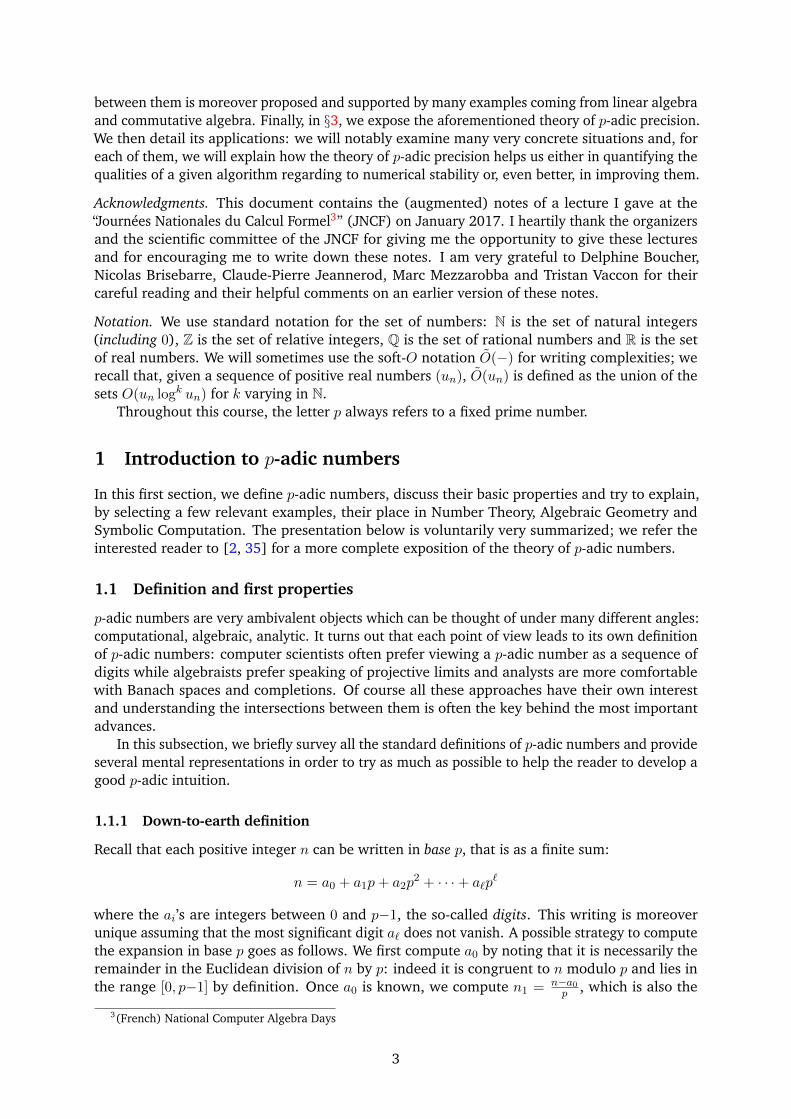
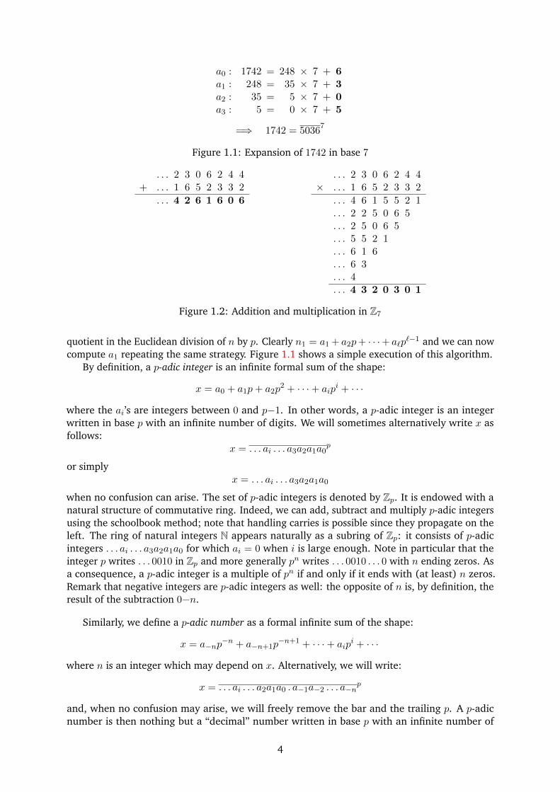
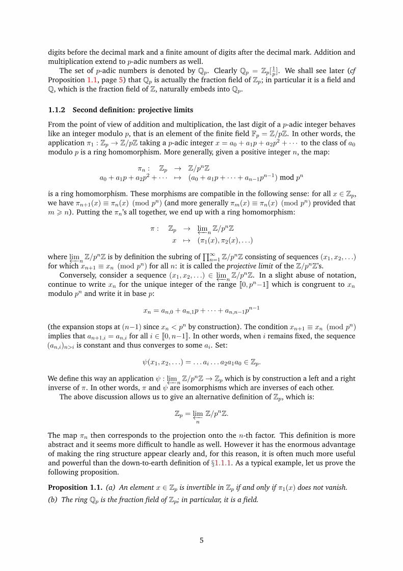


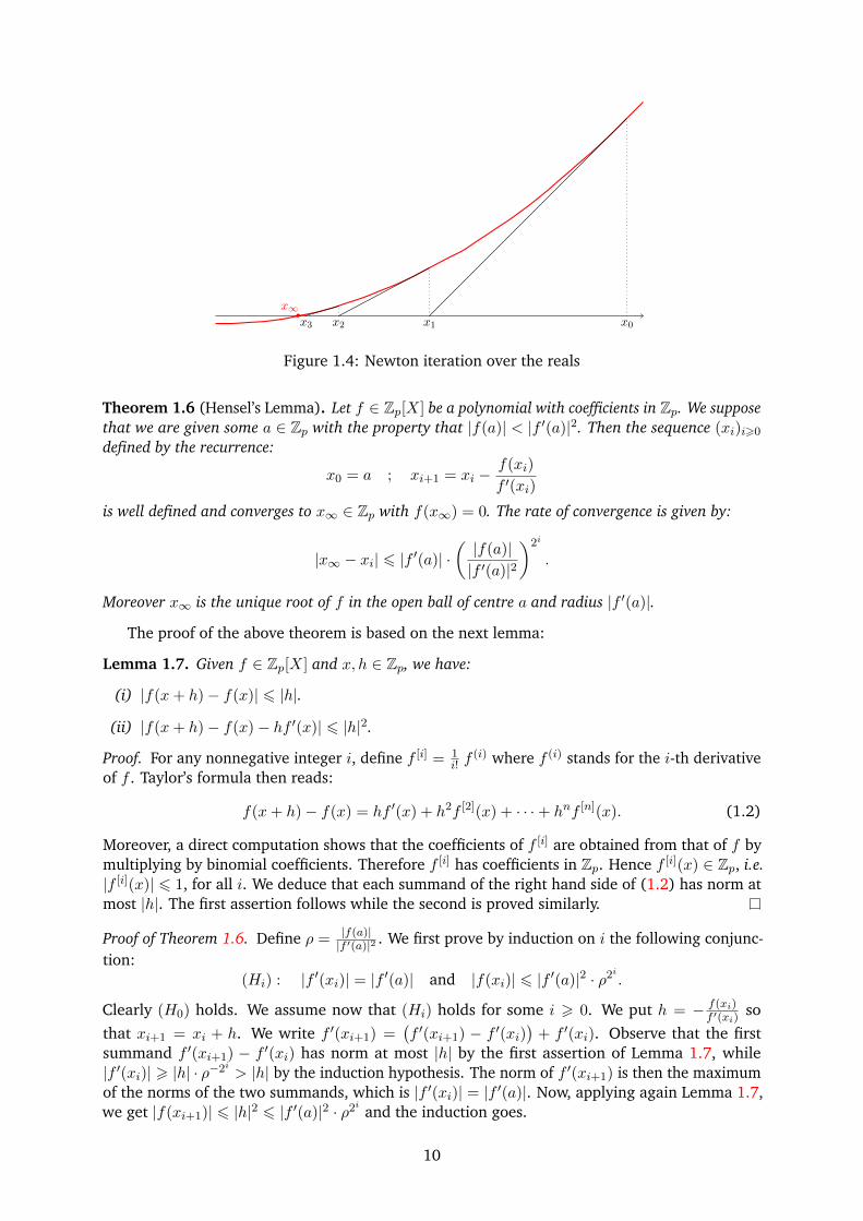
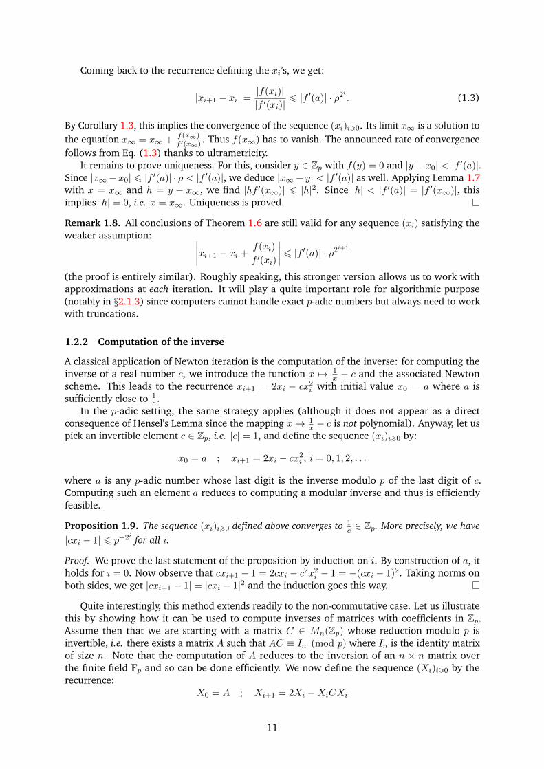
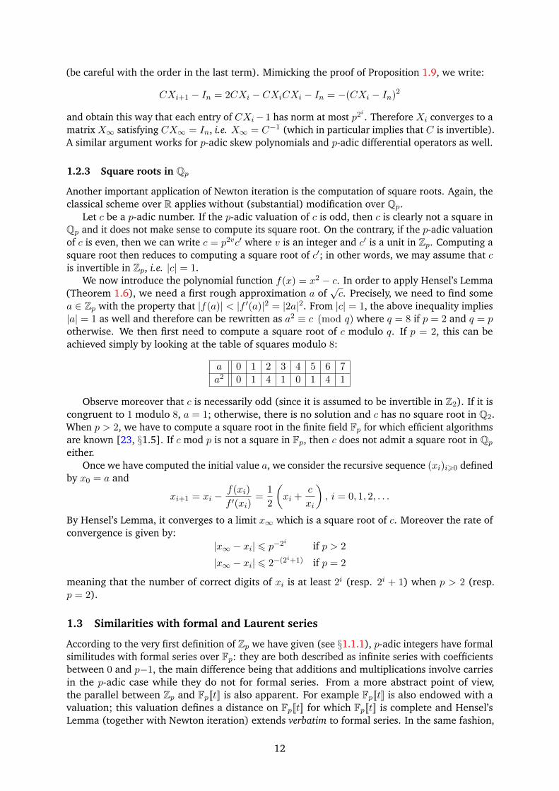
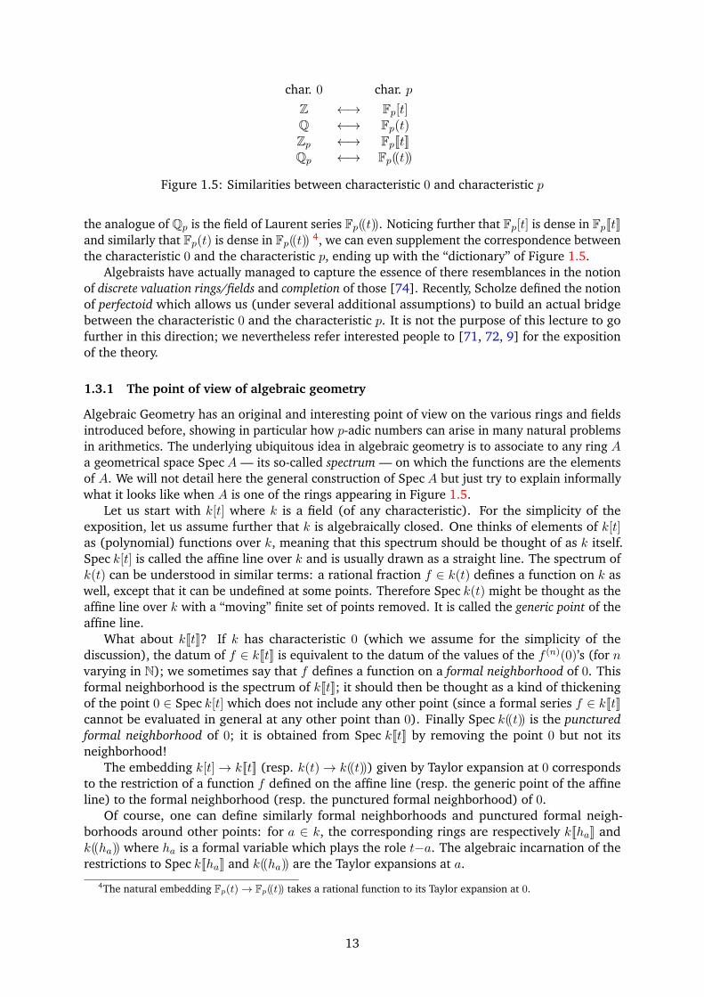
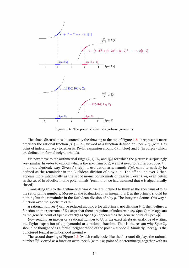


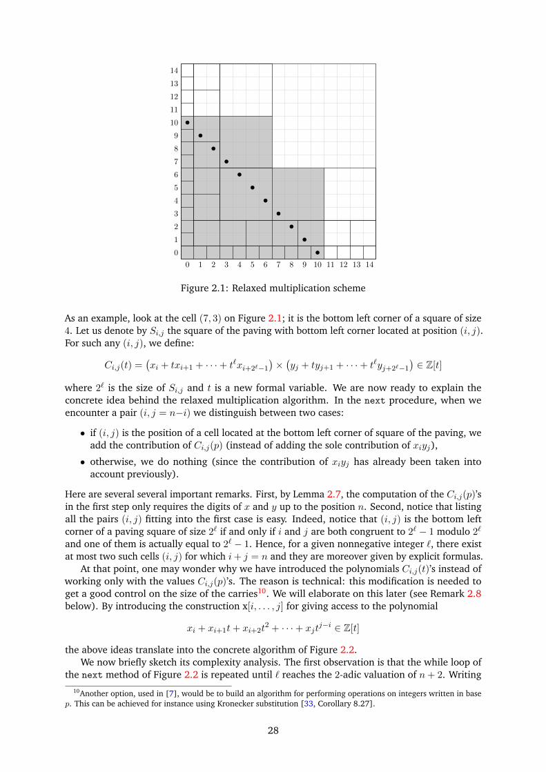

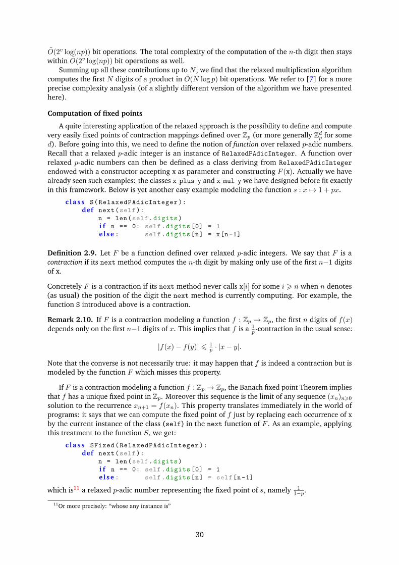


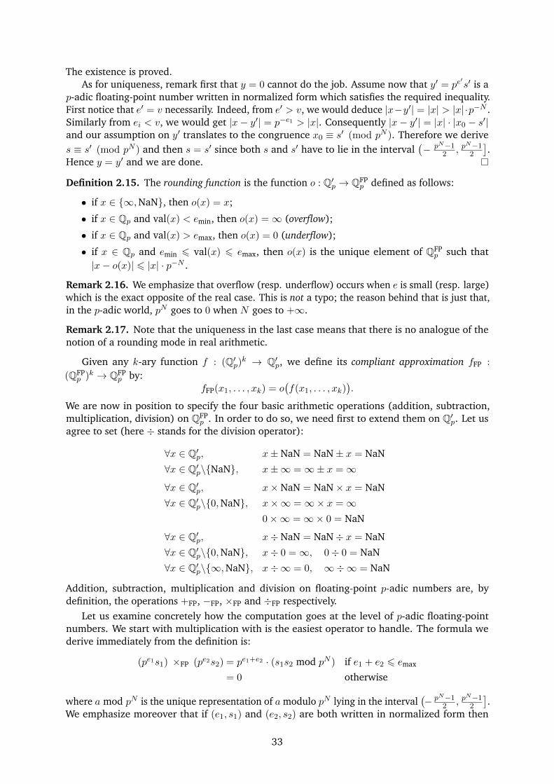
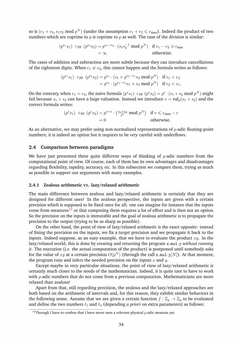

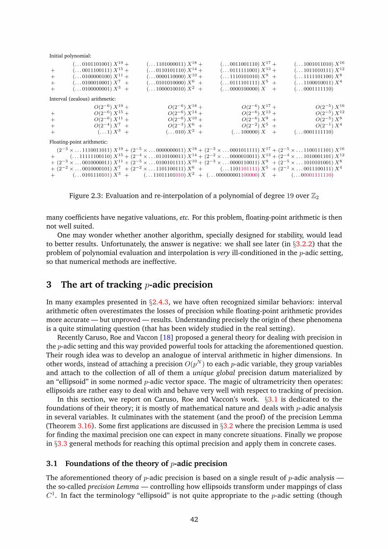


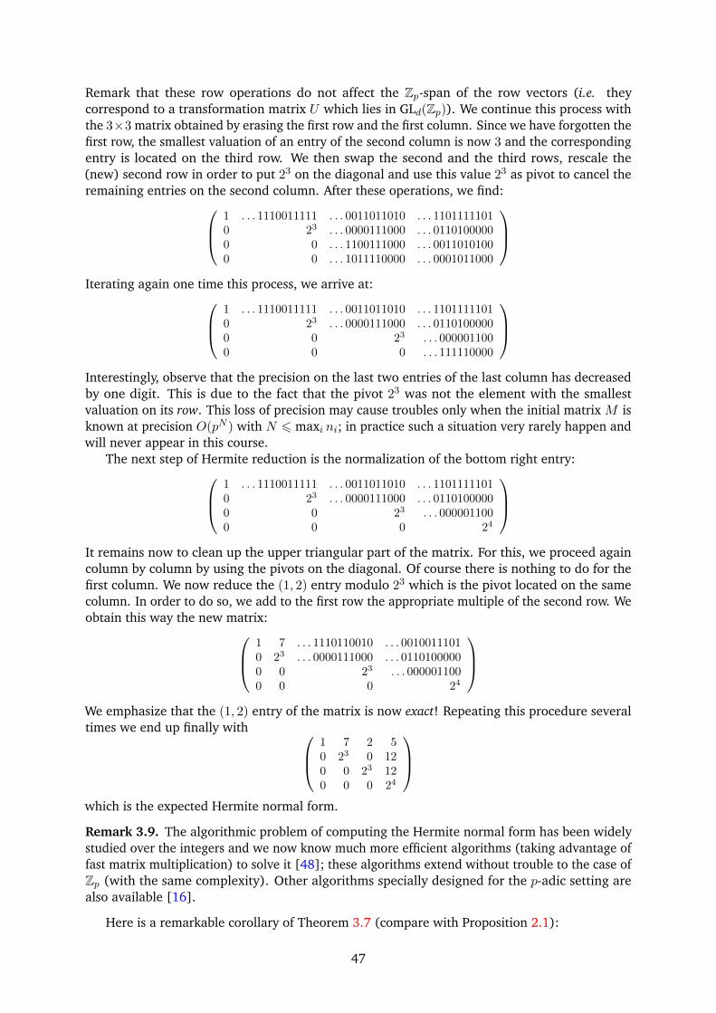

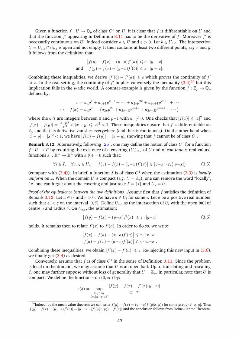
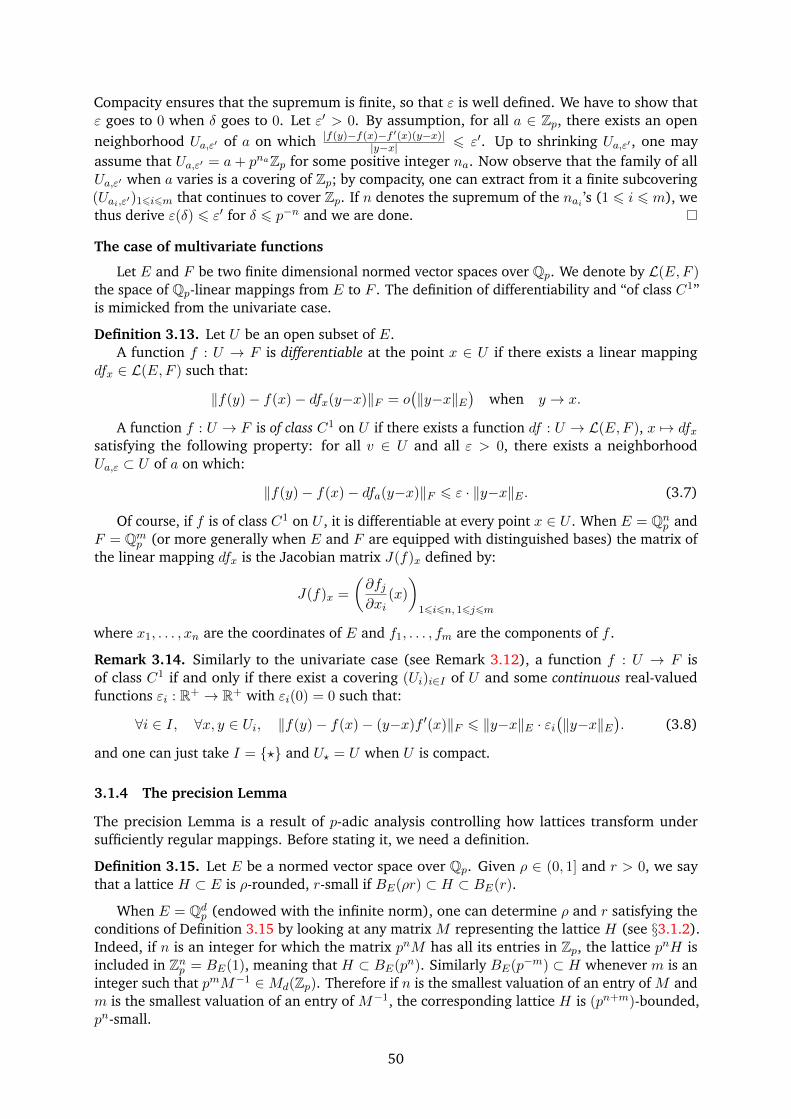
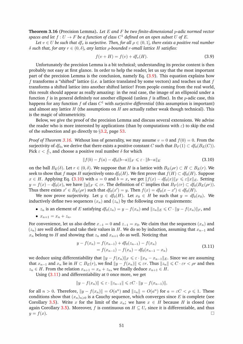


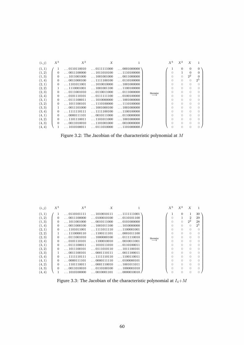
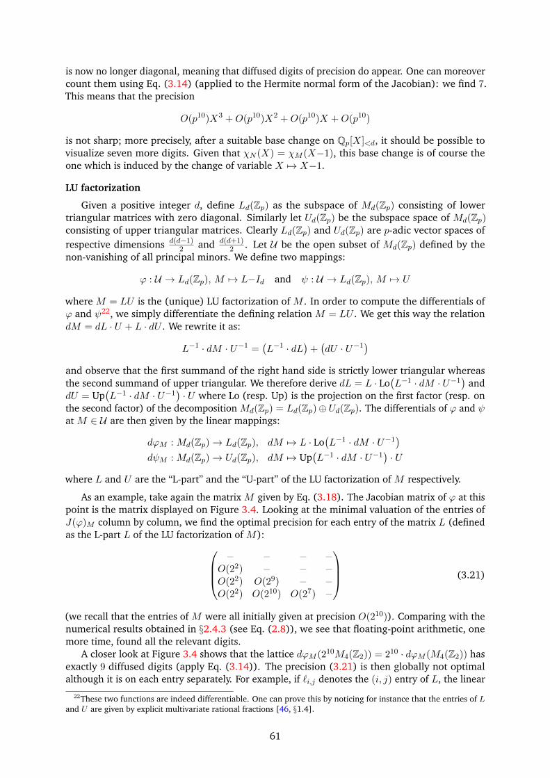

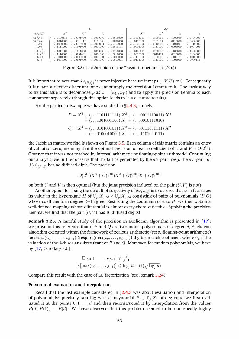


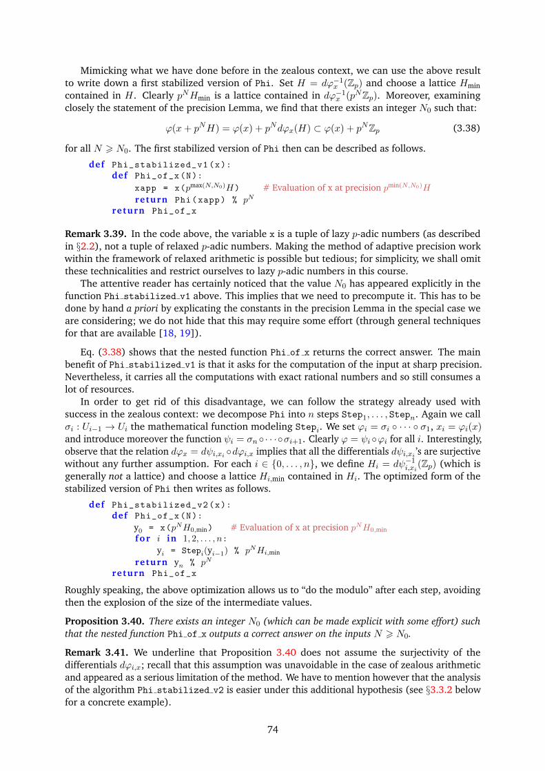
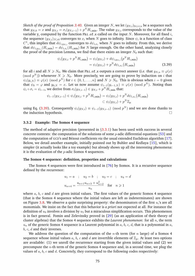

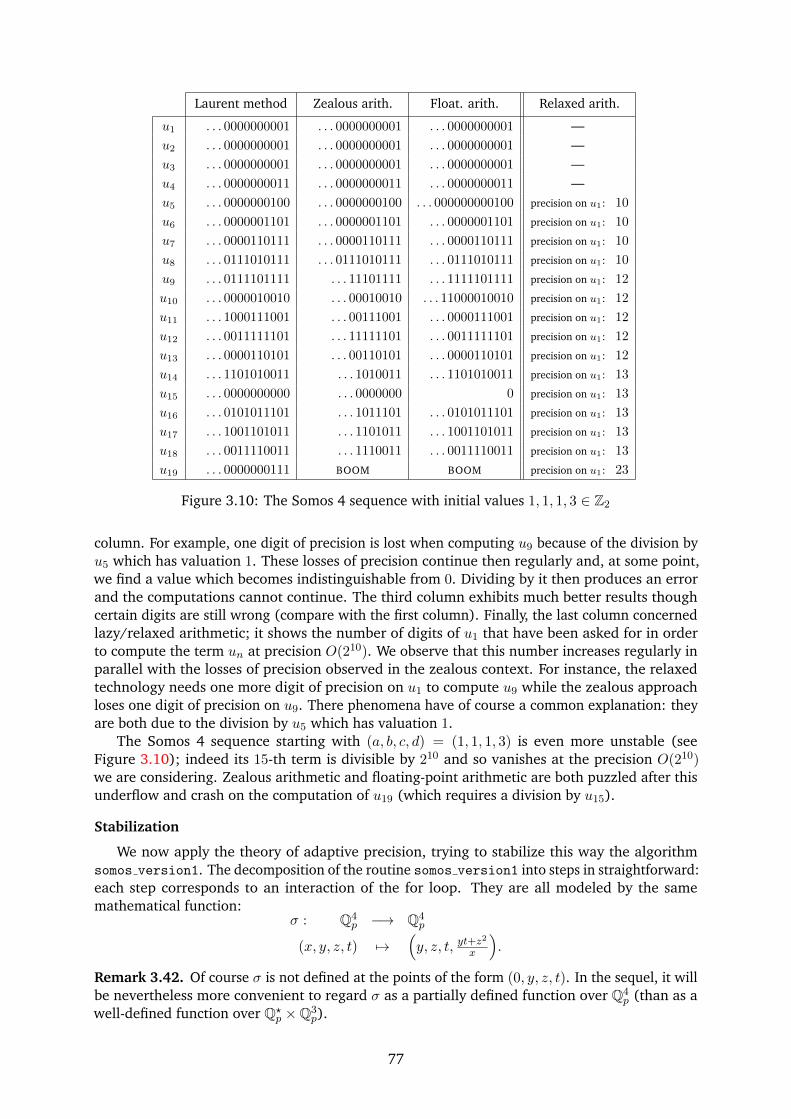

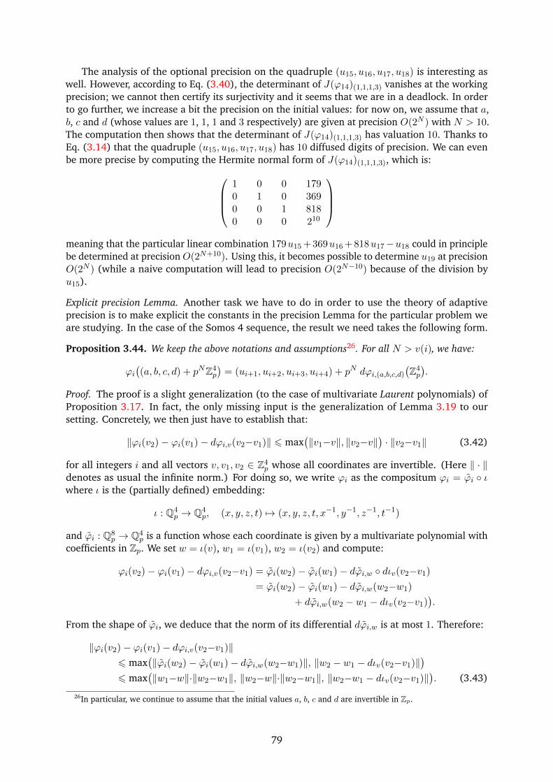
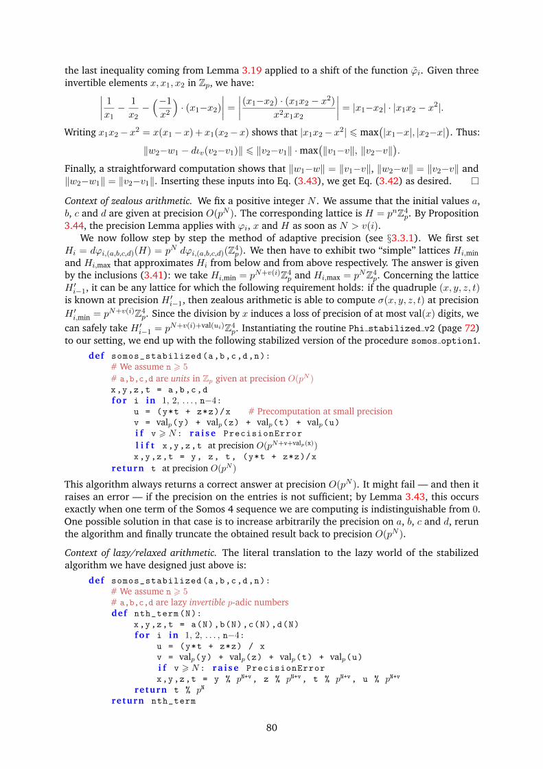


![-ADIC ELLIPTIC POLYLOGARITHM, -ADIC EISENSTEIN SERIES … · 2018-10-24 · arXiv:0707.3747v1 [math.NT] 25 Jul 2007 p-ADIC ELLIPTIC POLYLOGARITHM, p-ADIC EISENSTEIN SERIES AND KATZ](https://static.documents.pub/doc/80x56/5e26cc60ef471f7d09533bad/adic-elliptic-polylogarithm-adic-eisenstein-series-2018-10-24-arxiv07073747v1.jpg)