Computed and Experimental Flutter/LCO Onset for the Boeing Truss-Braced Wing Wind-Tunnel Model Robert E. Bartels * Robert C. Scott † Christie J. Funk ‡ NASA Langley Research Center, Hampton, VA Timothy J. Allen § Boeing Research and Technology, Huntington Beach, CA Bradley W. Sexton ¶ Boeing Research and Technology, St. Louis, MO This paper presents high fidelity Navier-Stokes simulations of the Boeing Subsonic Ultra Green Aircraft Research truss-braced wing wind-tunnel model and compares the results to linear MSC.Nastran flutter anal- ysis and preliminary data from a recent wind-tunnel test of that model at the NASA Langley Research Center Transonic Dynamics Tunnel. The simulated conditions under consideration are zero angle of attack, so that structural nonlinearity can be neglected. It is found that, for Mach numbers greater than 0.78, the linear flut- ter analysis predicts flutter onset dynamic pressure below that of the Navier-Stokes analysis and significantly below that found in the wind tunnel test. Furthermore, the wind-tunnel test revealed that the majority of the high structural dynamics cases were wing limit cycle oscillation (LCO) rather than flutter. Most Navier-Stokes simulated cases were also LCO rather than hard flutter. There is dip in the wind-tunnel test flutter/LCO onset in the Mach 0.76 - 0.80 range. Conditions tested above that Mach number exhibited no aeroelastic instability at the dynamic pressures reached in the tunnel. The linear flutter analyses do not show a flutter/LCO dip. The Navier-Stokes simulations reveal a slight dip in onset at Mach 0.82, then a significantly higher onset dynamic pressure at Mach 0.90. The Navier-Stokes simulations indicate a mild LCO onset at Mach 0.82, then a more rapidly growing instability at Mach 0.86 and 0.90. Finally, the modeling issues and their solution related to the use of a beam and pod finite element model to generate the Navier-Stokes structure mode shapes are discussed. I. Introduction The NASA Fixed Wing program has identified fuel efficiency and noise reduction targets as end products of funded research. To reach the goal of better fuel efficiency, propulsive and aerodynamic efficiency increases have been addressed in recent research efforts. The outcome of an N+3 phase 1 study conducted by the Boeing Company was the proposal to advance the Subsonic Ultra Green Aircraft Research (SUGAR) truss-braced wing (TBW) aircraft for further study. The advantages of the TBW configuration are its large aspect ratio, thin wings made possible by the added stiffness provided by a main and jury strut. The increase in aspect ratio results in a reduction of induced drag, while skin friction drag is reduced by maintaining laminar flow over thinner wings. One of the challenges of such a design is the likelihood of greater wing flexibility. This increased flexibility means that a multidisciplinary analysis of the vehicle aerodynamics, structure and control system is most likely required almost from the start of the design. The complexity of a wing/strut configuration designed to fly at a high subsonic Mach number suggests the use of higher fidelity tools to simulate the aerodynamic/structure interaction. The Boeing Company is just now completing an N+3 phase 2 study of the SUGAR TBW concept. 1, 2 This study included an analysis and design of a flight vehicle and the design and testing of an aeroelastic model in the NASA * Senior Aerospace Engineer, Aeroelasticity Branch, Senior Member. † Senior Aerospace Engineer, Aeroelasticity Branch, Associate Fellow. ‡ Aerospace Engineer, Aeroelasticity Branch, Member. § Principle Engineer. ¶ Principle Engineer, Associate Fellow. 1 of 24 American Institute of Aeronautics and Astronautics
Transcript
Computed and Experimental Flutter/LCO Onset for the BoeingTruss-Braced Wing Wind-Tunnel Model
Robert E. Bartels∗
Robert C. Scott†
Christie J. Funk‡
NASA Langley Research Center, Hampton, VA
Timothy J. Allen§
Boeing Research and Technology, Huntington Beach, CA
Bradley W. Sexton¶
Boeing Research and Technology, St. Louis, MO
This paper presents high fidelity Navier-Stokes simulations of the Boeing Subsonic Ultra Green AircraftResearch truss-braced wing wind-tunnel model and compares the results to linear MSC.Nastran flutter anal-ysis and preliminary data from a recent wind-tunnel test of that model at the NASA Langley Research CenterTransonic Dynamics Tunnel. The simulated conditions under consideration are zero angle of attack, so thatstructural nonlinearity can be neglected. It is found that, for Mach numbers greater than 0.78, the linear flut-ter analysis predicts flutter onset dynamic pressure below that of the Navier-Stokes analysis and significantlybelow that found in the wind tunnel test. Furthermore, the wind-tunnel test revealed that the majority of thehigh structural dynamics cases were wing limit cycle oscillation (LCO) rather than flutter. Most Navier-Stokessimulated cases were also LCO rather than hard flutter. There is dip in the wind-tunnel test flutter/LCO onsetin the Mach 0.76−0.80 range. Conditions tested above that Mach number exhibited no aeroelastic instabilityat the dynamic pressures reached in the tunnel. The linear flutter analyses do not show a flutter/LCO dip. TheNavier-Stokes simulations reveal a slight dip in onset at Mach 0.82, then a significantly higher onset dynamicpressure at Mach 0.90. The Navier-Stokes simulations indicate a mild LCO onset at Mach 0.82, then a morerapidly growing instability at Mach 0.86 and 0.90. Finally, the modeling issues and their solution related to theuse of a beam and pod finite element model to generate the Navier-Stokes structure mode shapes are discussed.
I. Introduction
The NASA Fixed Wing program has identified fuel efficiency and noise reduction targets as end products offunded research. To reach the goal of better fuel efficiency, propulsive and aerodynamic efficiency increases have beenaddressed in recent research efforts. The outcome of an N+3 phase 1 study conducted by the Boeing Company wasthe proposal to advance the Subsonic Ultra Green Aircraft Research (SUGAR) truss-braced wing (TBW) aircraft forfurther study. The advantages of the TBW configuration are its large aspect ratio, thin wings made possible by theadded stiffness provided by a main and jury strut. The increase in aspect ratio results in a reduction of induced drag,while skin friction drag is reduced by maintaining laminar flow over thinner wings. One of the challenges of such adesign is the likelihood of greater wing flexibility. This increased flexibility means that a multidisciplinary analysis ofthe vehicle aerodynamics, structure and control system is most likely required almost from the start of the design. Thecomplexity of a wing/strut configuration designed to fly at a high subsonic Mach number suggests the use of higherfidelity tools to simulate the aerodynamic/structure interaction.
The Boeing Company is just now completing an N+3 phase 2 study of the SUGAR TBW concept.1, 2 This studyincluded an analysis and design of a flight vehicle and the design and testing of an aeroelastic model in the NASA
American Institute of Aeronautics and Astronautics
Langley Research Center Transonic Dynamics Tunnel (TDT). The Boeing designed SUGAR TBW model was testedin the TDT in December 2013 and January-February 2014. The purpose of that test was to assess the open and closedloop aeroelastic stability of the SUGAR TBW model in an unperturbed and oscillating free stream and to obtain aflutter boundary as a function of Mach number and dynamic pressure. Comparisons of the TDT wind-tunnel flutteronset with nonlinear MSC.Nastran flutter onset recently have been presented.3 The present paper will compare andcontrast unsteady aeroelastic simulation results with the experimental data from the TDT test. For the present paper,the data of interest are the open loop flutter and limit cycle oscillation (LCO) onset boundaries in an unperturbed freestream. Low angle of attack conditions will be considered so that structural nonlinearity can be neglected.
The primary focus will be simulations performed with the unstructured FUN3D Navier-Stokes computational fluiddynamics (CFD) code. Before unsteady aeroelastic results can be shown, the technique developed here to effectthe fluid/structure data transfer will be discussed. The TDT wind-tunnel data to be presented in this paper will bediscussed. The finite element model and flutter onset simulation results using the Boeing MSC.Nastran linear modelof the SUGAR vehicle will be discussed. Finally CFD simulations of the vehicle aeroelastic response are presentedand compared to the doublet lattice method (DLM) and experimental data.
II. Wind-Tunnel Test Setup
A. Transonic Dynamics Tunnel
The Langley TDT is a unique national facility dedicated to identifying, understanding, and solving relevant aeroelasticand aeroservoelastic problems. The TDT is a closed circuit, continuous flow, variable pressure, wind-tunnel with a16 ft square test section with cropped corners.4 The tunnel uses either air or a heavy gas as the test medium and canoperate at total pressures from near vacuum to atmospheric. It has a Mach number range from near zero to 1.2 and iscapable of maximum unit Reynolds numbers of about 3 million per foot in air and 10 million per foot in heavy gas. TheTDT currently uses 1,1,1,2 tetrafluoroethane(R-134a)5, 6 as a heavy gas test medium. The TDT is specially configuredfor flutter testing, with excellent model visibility from the control room and a rapid tunnel shutdown capability formodel safety. Testing in heavy gas has important advantages over testing in air: improved model to full-scale similitude(which results in heavier, easier-to-build models with lower elastic mode frequencies), higher Reynolds numbers, andreduced tunnel power requirements. Results presented are at nominal angles of attack in the range −1 ≤ α ≤ 1, Machnumbers in the range 0.70 ≤ M ≤ 0.80 corresponding to Reynolds numbers of roughly 1 million to 2 million based onmean aerodynamic chord.
B. Wind-Tunnel Model
The SUGAR TBW wind-tunnel model is a 15 percent semispan side wall mounted model. The SUGAR TBW conceptwas developed by The Boeing Company and is described in reference 1. The wing and mount system for the SUGARTBW test were designed and fabricated by NextGen Aeronautics in Torrance, California. NextGen Aeronautics was asubcontractor to The Boeing Company. Details can be found in reference 2. The model includes main and jury struts,pylon and annular nacelle, wing and fuselage. The vehicle empennage is not included in the wind-tunnel model. Thefuselage includes an offset to bring the entire fuselage/wing outside the wind-tunnel wall boundary layer. The wing andstruts are composed of spars for load bearing and pods to provide aerodynamic shape. The model is aeroelasticallyscaled for testing in heavy gas which, in addition to the advantages enumerated in the previous section, minimizesactuator bandwidth requirements.
Figure 1 shows a photo of the SUGAR TBW model installed in the TDT. The scaled fuselage length was 18.8ft, but it was shortened to 13.4 ft to reduce weight and potential torsional dynamics with the turntable mount. Themean aerodynamic chord is 16.5 inches. The model wing span to the center line is 12.75 ft (about 75 percent ofthe tunnel width) with an additional 2.25 inches added to the half fuselage, the approximate wind-tunnel boundarylayer displacement thickness. The wing, strut and jury use a spar-pod design where the scaled stiffnesses (EI andGJ distributions) are designed into the flanged aluminum spar, and the aerodynamic shape is provided by discretefairings, or pods, mounted to the spars. The pods were made of graphite epoxy and attached to the spars using brackets.The nacelle and pylon are not structurally scaled, but have the correct mass and inertia. The fuselage consists of analuminum internal structure with fiberglass skin panels. Lead weights are attached to the wing spar in several locationsso the wing has the proper scaled mass.
One of the the objectives of the SUGAR TBW test was to demonstrate flutter suppression. As a result, the winghas two trailing edge control surfaces, one near the wing tip and one just outboard of the engine pylon. Each aileron is
2 of 24
American Institute of Aeronautics and Astronautics
driven by a vane-type hydraulic actuator with position measured by a rotary variable differential transducer (RVDT).Other instrumentation included 11 strain gauges and 21 accelerometers. The model was supported by a turntable onthe east wall of the TDT as shown in Figure 1, and the model angle of attack was varied between -3 and +5 degrees.
III. Computational Model Development
A. Finite Element Structural Model
Several MSC.Nastran finite element models (FEMs) of the SUGAR TBW configuration were generated over thecourse of this project. A full-scale, full-span version with highly detailed wing structure FEM was used in the de-sign/optimization studies described in reference 1. As part of the aeroelastic wind-tunnel model development processseveral semi-span, beam-rod FEMs were also developed. This FEM was refined as the details of the model structuraldesign matured. The scaled mass and stiffness are reflected in version 19 of the beam-rod FEM shown in Figure 2a.This FEM includes updates to produce a good correlation with in-tunnel ground vibration test (GVT) measured modalfrequencies and mode shapes. The structural damping has also been estimated from GVT to be around one percent.Note that a version 20 FEM with a better correlation with GVT data is now available, but is not used in this study.
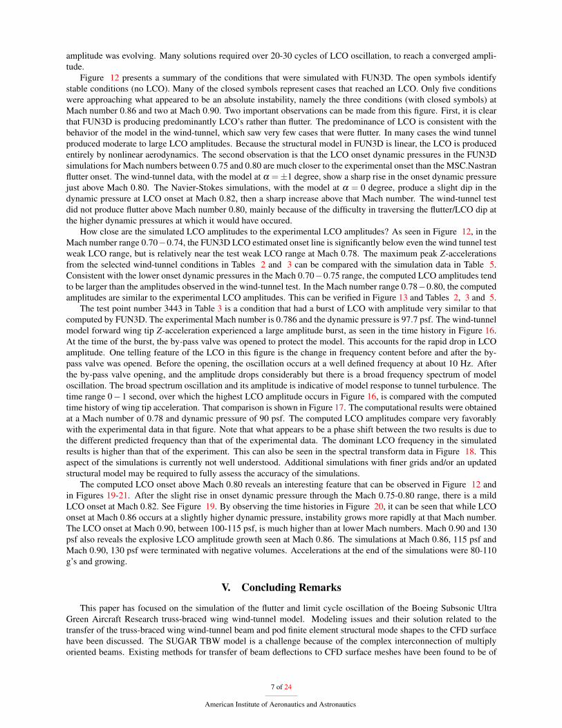
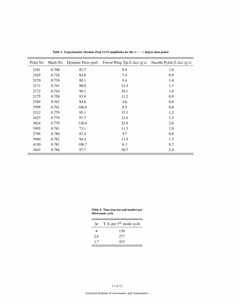
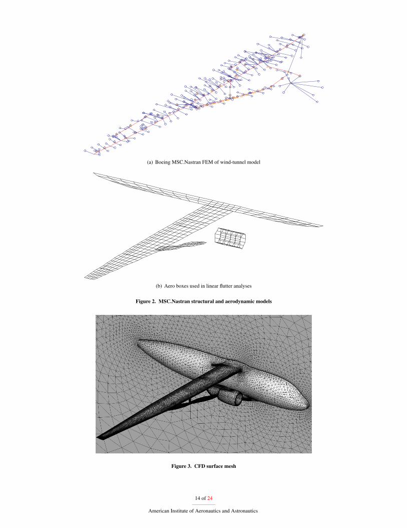
Version 19 of the beam-rod FEM has approximately 400 nodes with 200 elements including CBEAM, CONM2,RBAR , and RBE2 element types. This model consists of beams for the wing and strut spars, engine strut and controlsurface hinges. Discrete weights such as control surface actuators, spar/wing and engine spar/wing attachments areconnected to the various beams by rigid body elements. Structural displacements are thus produced at a fairly complexarrangement of isolated node points. Accelerometer and strain gauge locations consistent with the physical modelare included. Figure 2b shows the doublet lattice aerodynamic box layout used for the linear flutter analyses. Theaerodynamic model was linked to the structural model using a combination of infinite plate and infinite beam splines.There are four major spline regions for the four major aero groups seen in Figure 2b: engine/nacelle, wing, strut, andfuselage. Also, each control surface has spline points associated with them as well. Additional modeling details canbe found in reference 2 and a version of this FEM was used in the study described in reference 3. Both the linear andhigh fidelity nonlinear simulations discussed here use the normal structural modes from a vehicle finite element modelthat does not include any pre-stress. Modal frequencies for the first 16 modes are shown in Table 1. It can be seenthat the first five modes include a variety of in-plane and out-of-plane wing bending and wing/nacelle torsion. Higherfrequency modes also include strut bending and strut torsion.
B. High Fidelity Nonlinear Computational Fluid Dynamics Model
The high fidelity simulations are performed by the FUN3D CFD code. The Navier-Stokes code FUN3D (fully un-structured Navier-Stokes three-dimensional) is a finite-volume unstructured CFD code.8 Flow variables are stored atthe vertices of the grid. The compressible Reynolds-averaged Navier-Stokes (RANS) flow equations and the Spalart-Allmaras turbulence model are solved on a tetrahedral grid. The Venkatakrishnan flux limiter is used and flux con-struction is performed by the low dissipation scheme.
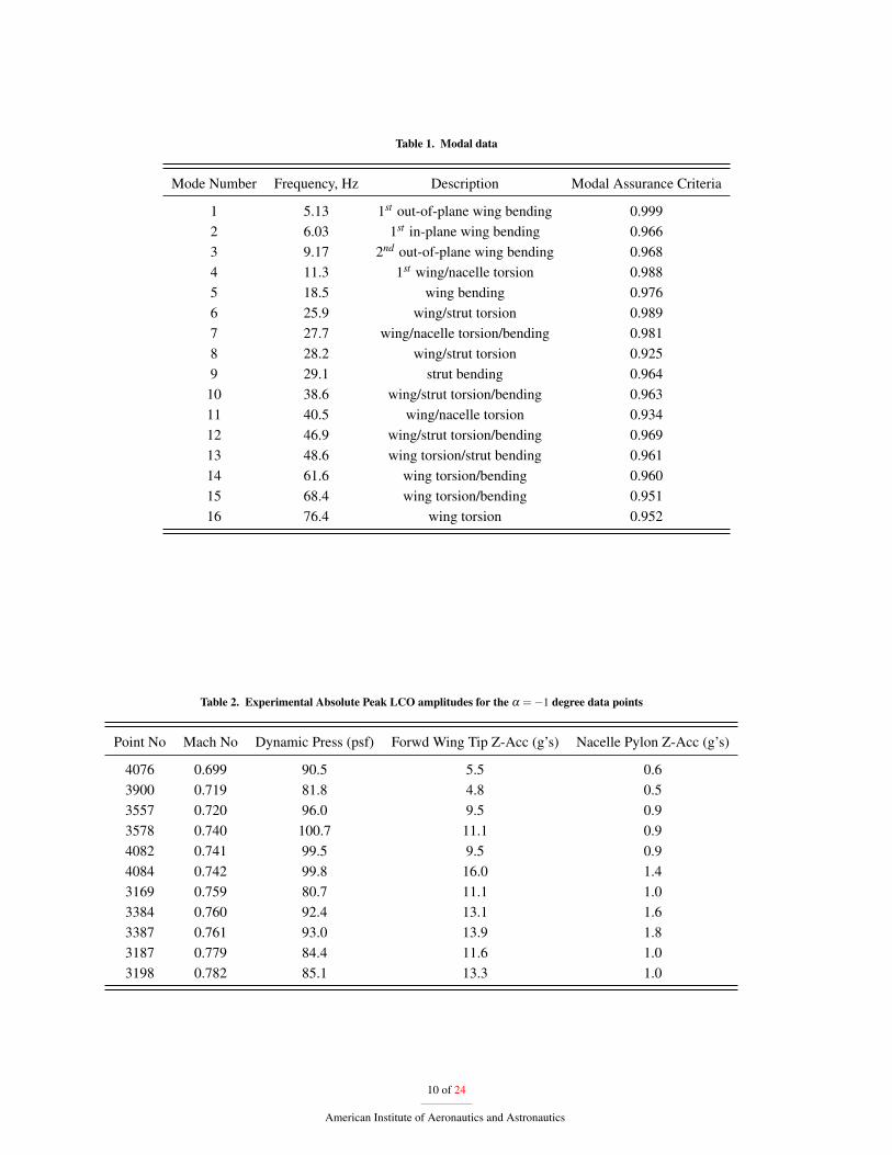
The SUGAR TBW surface mesh used in the FUN3D calculations is shown in Figure 3. A semi-infinite tetrahedralvolume grid having 4.5 million nodes was developed with the VGRID software.7 The wind-tunnel wall is treatedas a symmetry plane. As in the wind-tunnel model, an offset has been added to account for the effect of the tunnelwall boundary layer. Upstream, downstream and side boundaries are placed at 10 wing span lengths from the model.Normal spacing of the first grid point off the vehicle surface is at y+ ≈ 1 everywhere.
Steady state and subiterative solutions are accelerated to convergence by the use of local time stepping.8 Domaindecomposition is used to enable distributed parallel computing. The solutions are computed on 288−800 processorsdepending on the platform.
The aeroelastic simulations in this paper use mode shapes internal to the FUN3D code coupled with the generalizedequations of structural dynamics. For a moving mesh, the conservation equations are written in the Arbitrary LagrangeEuler (ALE) formulation.9 The mesh deformation is accomplished by treating the mesh motion as analogous to a linearelasticity problem. The material properties vary based on distance to the nearest solid boundary. Elements near a solidboundary are made significantly stiffer by specifying the value of the Youngs modulus (E).
3 of 24
American Institute of Aeronautics and Astronautics
C. Force and Deflection Transfer Between Dissimilar Structure/CFD Models
A key step in performing aeroelastic analysis is the transfer of structural deflections and fluid forces between thestructure and the CFD surface nodes. Methods have been developed based on various interpolation and finite elementshape functions. To name a few examples in use, there is the inverse isoparametric mapping,10 third order spline,11
nonuniform B-splines or those based on quadric surface basis functions.12 In the case of the FUN3D fluid/structureinteraction, the Discrete Data Transfer Between Dissimilar Models (DDTBDM) software13 is often employed. Thatsoftware uses a derivative of the inverse isoparametric mapping algorithm presented by Farhat, Lesoinne, and LeTal-lec.14 This method works well when the target and source nodes are in reasonably close proximity.
As discussed earlier, the SUGAR TBW model fuselage, wing, trusses and nacelle pylon are modeled structurallyby a collection of flexible and rigid beams with discrete masses. To accomodate the fluid/structure transfer for thesevarious elements, the Boeing MSC.Nastran SUGAR model defines four infinite plate splines (IPS)15 and the beamnodes and aerodynamic boxes associated with each of these splines. Because the FEM structure and DLM aerodynamicmodels have similar coarse node spacing, it is straightforward to define spline regions that encompass all the structureand aerodynamic nodes. Furthermore, in the current DLM aerodynamic model, the wing and strut and nacelle boxesare not connected (see Figure 2). Different splines can be defined without discontinuities appearing between splineregions. It is more challenging when the structure FEM and CFD node spacings widely differ. Particularly, when thecontinuous CFD surface mesh has very tight grid spacing between several splined regions, any discontinuities at splineregion intersections will be transmitted to the CFD surface. Such discontinuities in a CFD surface mesh are, of course,not tolerated.
Methods of interfacing beam models with CFD surfaces that use an extrapolation of beam nodal displacements androtations have been in existence for some time.16, 17 Using this approach, it is possible to extrapolate beam deflectionsusing rigid body rotations and translations to CFD nodes that are far from the associated beam node. This approachhas been very successful for applications such as an isolated rotor blade or wing where the transfer is between a simplebeam and its associated CFD surface.18, 19, 20 The DDTBDM software also has this capability to transfer between afairly simple beam model and a CFD surface mesh.
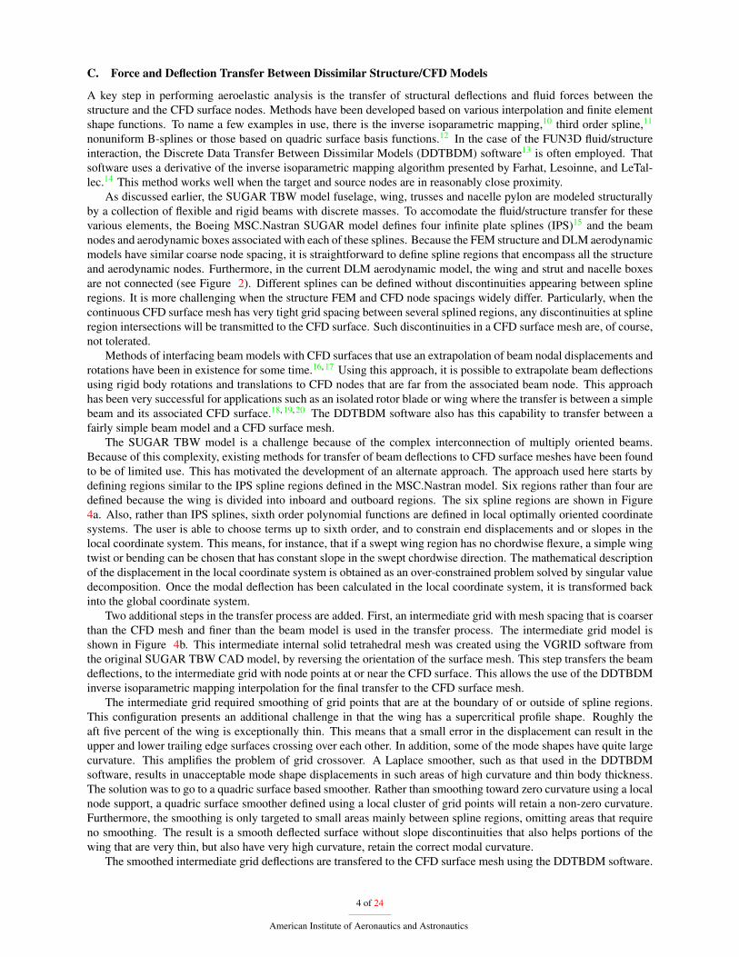
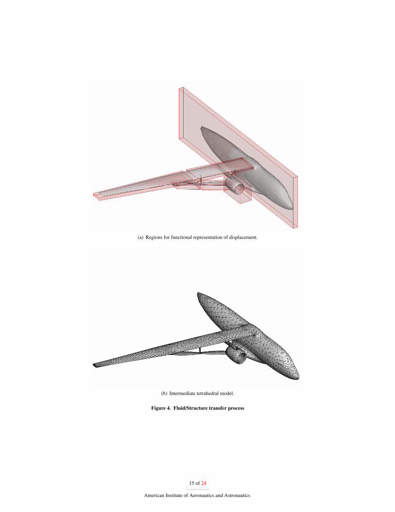
The SUGAR TBW model is a challenge because of the complex interconnection of multiply oriented beams.Because of this complexity, existing methods for transfer of beam deflections to CFD surface meshes have been foundto be of limited use. This has motivated the development of an alternate approach. The approach used here starts bydefining regions similar to the IPS spline regions defined in the MSC.Nastran model. Six regions rather than four aredefined because the wing is divided into inboard and outboard regions. The six spline regions are shown in Figure4a. Also, rather than IPS splines, sixth order polynomial functions are defined in local optimally oriented coordinatesystems. The user is able to choose terms up to sixth order, and to constrain end displacements and or slopes in thelocal coordinate system. This means, for instance, that if a swept wing region has no chordwise flexure, a simple wingtwist or bending can be chosen that has constant slope in the swept chordwise direction. The mathematical descriptionof the displacement in the local coordinate system is obtained as an over-constrained problem solved by singular valuedecomposition. Once the modal deflection has been calculated in the local coordinate system, it is transformed backinto the global coordinate system.
Two additional steps in the transfer process are added. First, an intermediate grid with mesh spacing that is coarserthan the CFD mesh and finer than the beam model is used in the transfer process. The intermediate grid model isshown in Figure 4b. This intermediate internal solid tetrahedral mesh was created using the VGRID software fromthe original SUGAR TBW CAD model, by reversing the orientation of the surface mesh. This step transfers the beamdeflections, to the intermediate grid with node points at or near the CFD surface. This allows the use of the DDTBDMinverse isoparametric mapping interpolation for the final transfer to the CFD surface mesh.
The intermediate grid required smoothing of grid points that are at the boundary of or outside of spline regions.This configuration presents an additional challenge in that the wing has a supercritical profile shape. Roughly theaft five percent of the wing is exceptionally thin. This means that a small error in the displacement can result in theupper and lower trailing edge surfaces crossing over each other. In addition, some of the mode shapes have quite largecurvature. This amplifies the problem of grid crossover. A Laplace smoother, such as that used in the DDTBDMsoftware, results in unacceptable mode shape displacements in such areas of high curvature and thin body thickness.The solution was to go to a quadric surface based smoother. Rather than smoothing toward zero curvature using a localnode support, a quadric surface smoother defined using a local cluster of grid points will retain a non-zero curvature.Furthermore, the smoothing is only targeted to small areas mainly between spline regions, omitting areas that requireno smoothing. The result is a smooth deflected surface without slope discontinuities that also helps portions of thewing that are very thin, but also have very high curvature, retain the correct modal curvature.
The smoothed intermediate grid deflections are transfered to the CFD surface mesh using the DDTBDM software.
4 of 24
American Institute of Aeronautics and Astronautics
It was also found that the inverse isoparametric interpolation would produce, in areas of high curvature (e.g. in somestrut modes), slightly perceptible triangular faceting corresponding to the triangular surfaces of the intermediate gridtetrahedra. Once again, targeted smoothing was applied using the quadric surface smoother. Targeting small regionsof the vehicle is intended to reduce as much as possible the degrading effect the smoothing has on the transfered themode shape.
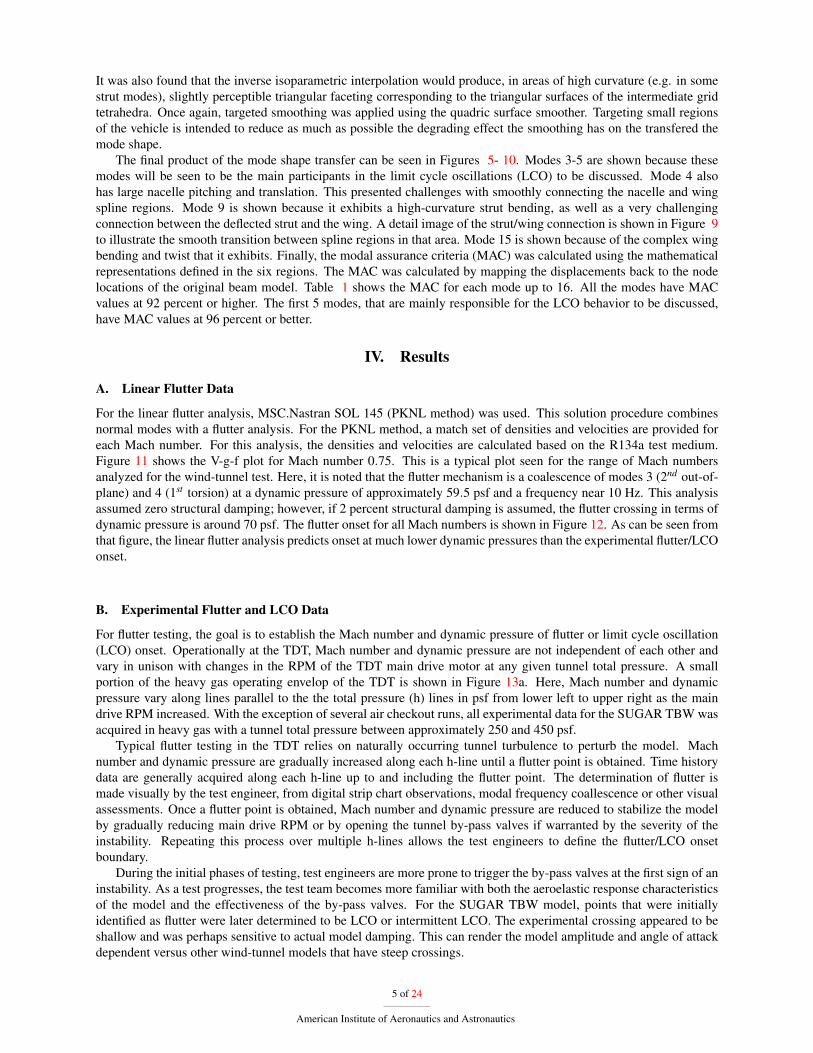
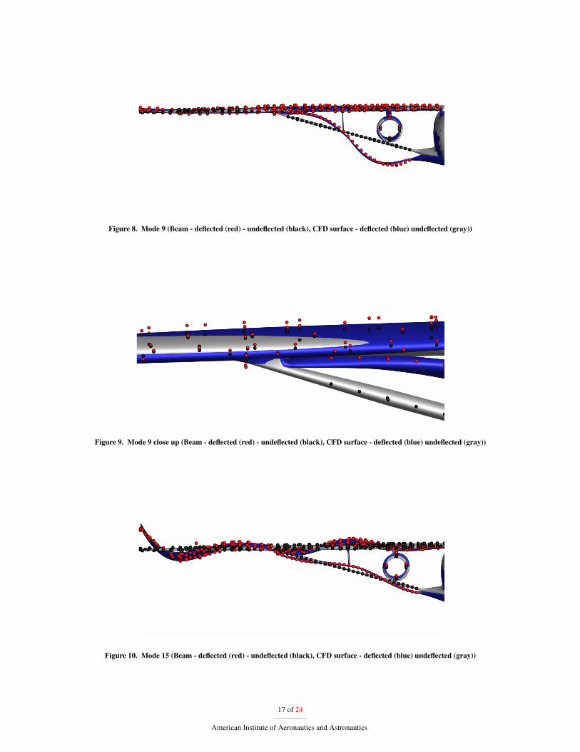
The final product of the mode shape transfer can be seen in Figures 5- 10. Modes 3-5 are shown because thesemodes will be seen to be the main participants in the limit cycle oscillations (LCO) to be discussed. Mode 4 alsohas large nacelle pitching and translation. This presented challenges with smoothly connecting the nacelle and wingspline regions. Mode 9 is shown because it exhibits a high-curvature strut bending, as well as a very challengingconnection between the deflected strut and the wing. A detail image of the strut/wing connection is shown in Figure 9to illustrate the smooth transition between spline regions in that area. Mode 15 is shown because of the complex wingbending and twist that it exhibits. Finally, the modal assurance criteria (MAC) was calculated using the mathematicalrepresentations defined in the six regions. The MAC was calculated by mapping the displacements back to the nodelocations of the original beam model. Table 1 shows the MAC for each mode up to 16. All the modes have MACvalues at 92 percent or higher. The first 5 modes, that are mainly responsible for the LCO behavior to be discussed,have MAC values at 96 percent or better.
IV. Results
A. Linear Flutter Data
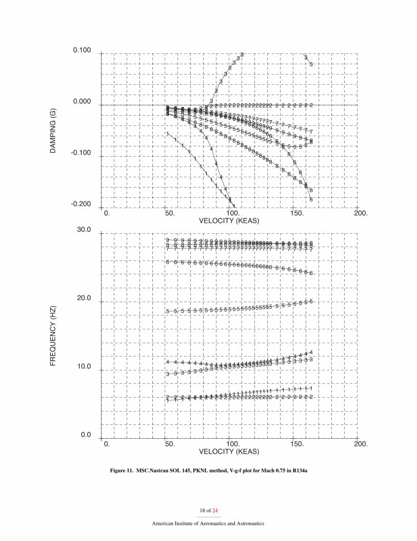
For the linear flutter analysis, MSC.Nastran SOL 145 (PKNL method) was used. This solution procedure combinesnormal modes with a flutter analysis. For the PKNL method, a match set of densities and velocities are provided foreach Mach number. For this analysis, the densities and velocities are calculated based on the R134a test medium.Figure 11 shows the V-g-f plot for Mach number 0.75. This is a typical plot seen for the range of Mach numbersanalyzed for the wind-tunnel test. Here, it is noted that the flutter mechanism is a coalescence of modes 3 (2nd out-of-plane) and 4 (1st torsion) at a dynamic pressure of approximately 59.5 psf and a frequency near 10 Hz. This analysisassumed zero structural damping; however, if 2 percent structural damping is assumed, the flutter crossing in terms ofdynamic pressure is around 70 psf. The flutter onset for all Mach numbers is shown in Figure 12. As can be seen fromthat figure, the linear flutter analysis predicts onset at much lower dynamic pressures than the experimental flutter/LCOonset.
B. Experimental Flutter and LCO Data
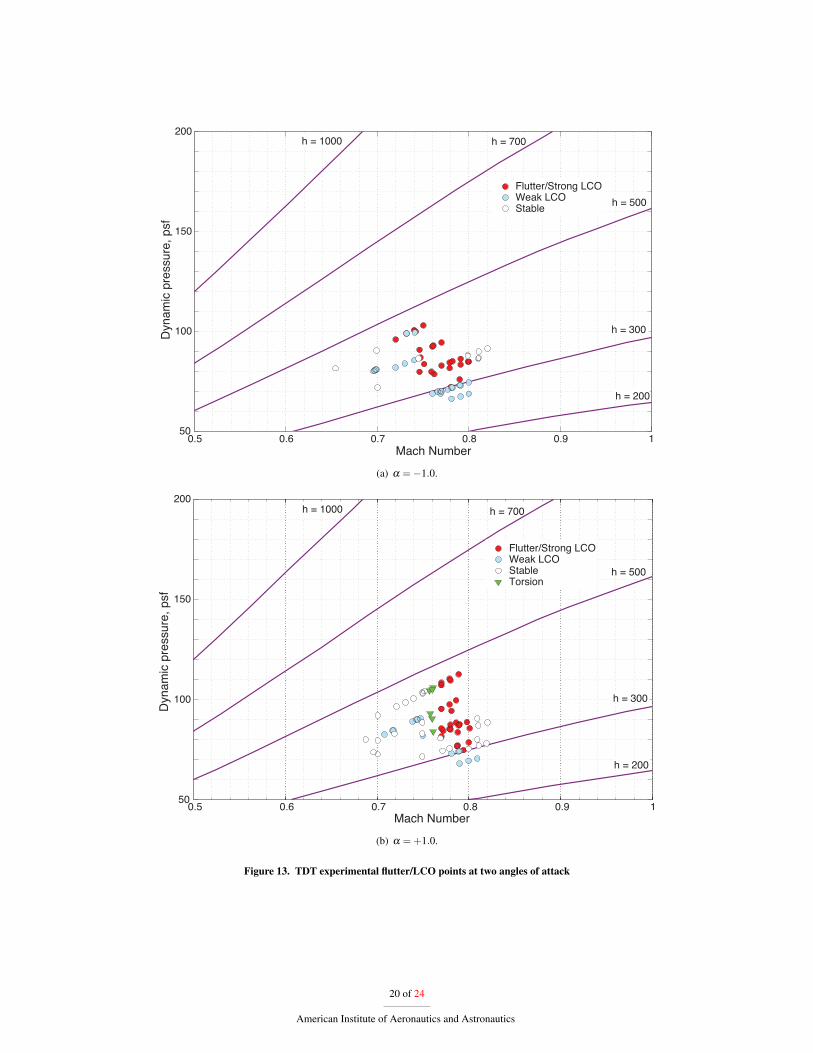
For flutter testing, the goal is to establish the Mach number and dynamic pressure of flutter or limit cycle oscillation(LCO) onset. Operationally at the TDT, Mach number and dynamic pressure are not independent of each other andvary in unison with changes in the RPM of the TDT main drive motor at any given tunnel total pressure. A smallportion of the heavy gas operating envelop of the TDT is shown in Figure 13a. Here, Mach number and dynamicpressure vary along lines parallel to the the total pressure (h) lines in psf from lower left to upper right as the maindrive RPM increased. With the exception of several air checkout runs, all experimental data for the SUGAR TBW wasacquired in heavy gas with a tunnel total pressure between approximately 250 and 450 psf.
Typical flutter testing in the TDT relies on naturally occurring tunnel turbulence to perturb the model. Machnumber and dynamic pressure are gradually increased along each h-line until a flutter point is obtained. Time historydata are generally acquired along each h-line up to and including the flutter point. The determination of flutter ismade visually by the test engineer, from digital strip chart observations, modal frequency coallescence or other visualassessments. Once a flutter point is obtained, Mach number and dynamic pressure are reduced to stabilize the modelby gradually reducing main drive RPM or by opening the tunnel by-pass valves if warranted by the severity of theinstability. Repeating this process over multiple h-lines allows the test engineers to define the flutter/LCO onsetboundary.
During the initial phases of testing, test engineers are more prone to trigger the by-pass valves at the first sign of aninstability. As a test progresses, the test team becomes more familiar with both the aeroelastic response characteristicsof the model and the effectiveness of the by-pass valves. For the SUGAR TBW model, points that were initiallyidentified as flutter were later determined to be LCO or intermittent LCO. The experimental crossing appeared to beshallow and was perhaps sensitive to actual model damping. This can render the model amplitude and angle of attackdependent versus other wind-tunnel models that have steep crossings.
5 of 24
American Institute of Aeronautics and Astronautics
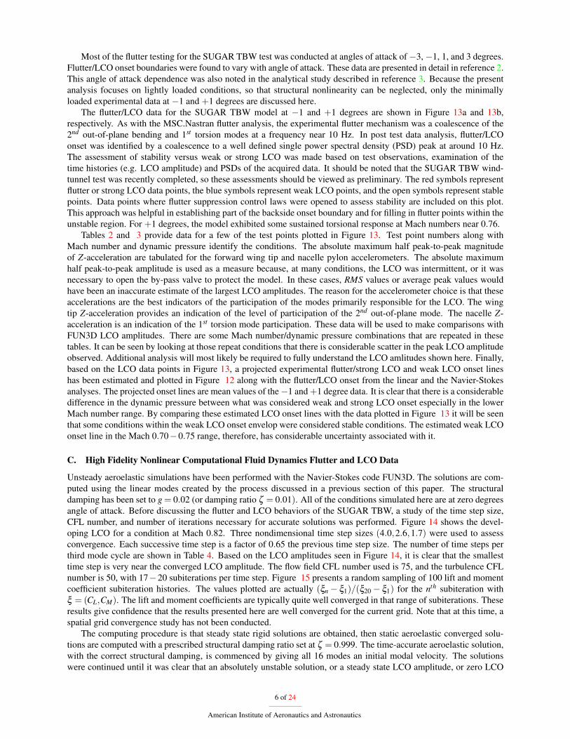
Most of the flutter testing for the SUGAR TBW test was conducted at angles of attack of −3, −1, 1, and 3 degrees.Flutter/LCO onset boundaries were found to vary with angle of attack. These data are presented in detail in reference 2.This angle of attack dependence was also noted in the analytical study described in reference 3. Because the presentanalysis focuses on lightly loaded conditions, so that structural nonlinearity can be neglected, only the minimallyloaded experimental data at −1 and +1 degrees are discussed here.
The flutter/LCO data for the SUGAR TBW model at −1 and +1 degrees are shown in Figure 13a and 13b,respectively. As with the MSC.Nastran flutter analysis, the experimental flutter mechanism was a coalescence of the2nd out-of-plane bending and 1st torsion modes at a frequency near 10 Hz. In post test data analysis, flutter/LCOonset was identified by a coalescence to a well defined single power spectral density (PSD) peak at around 10 Hz.The assessment of stability versus weak or strong LCO was made based on test observations, examination of thetime histories (e.g. LCO amplitude) and PSDs of the acquired data. It should be noted that the SUGAR TBW wind-tunnel test was recently completed, so these assessments should be viewed as preliminary. The red symbols representflutter or strong LCO data points, the blue symbols represent weak LCO points, and the open symbols represent stablepoints. Data points where flutter suppression control laws were opened to assess stability are included on this plot.This approach was helpful in establishing part of the backside onset boundary and for filling in flutter points within theunstable region. For +1 degrees, the model exhibited some sustained torsional response at Mach numbers near 0.76.
Tables 2 and 3 provide data for a few of the test points plotted in Figure 13. Test point numbers along withMach number and dynamic pressure identify the conditions. The absolute maximum half peak-to-peak magnitudeof Z-acceleration are tabulated for the forward wing tip and nacelle pylon accelerometers. The absolute maximumhalf peak-to-peak amplitude is used as a measure because, at many conditions, the LCO was intermittent, or it wasnecessary to open the by-pass valve to protect the model. In these cases, RMS values or average peak values wouldhave been an inaccurate estimate of the largest LCO amplitudes. The reason for the accelerometer choice is that theseaccelerations are the best indicators of the participation of the modes primarily responsible for the LCO. The wingtip Z-acceleration provides an indication of the level of participation of the 2nd out-of-plane mode. The nacelle Z-acceleration is an indication of the 1st torsion mode participation. These data will be used to make comparisons withFUN3D LCO amplitudes. There are some Mach number/dynamic pressure combinations that are repeated in thesetables. It can be seen by looking at those repeat conditions that there is considerable scatter in the peak LCO amplitudeobserved. Additional analysis will most likely be required to fully understand the LCO amlitudes shown here. Finally,based on the LCO data points in Figure 13, a projected experimental flutter/strong LCO and weak LCO onset lineshas been estimated and plotted in Figure 12 along with the flutter/LCO onset from the linear and the Navier-Stokesanalyses. The projected onset lines are mean values of the −1 and +1 degree data. It is clear that there is a considerabledifference in the dynamic pressure between what was considered weak and strong LCO onset especially in the lowerMach number range. By comparing these estimated LCO onset lines with the data plotted in Figure 13 it will be seenthat some conditions within the weak LCO onset envelop were considered stable conditions. The estimated weak LCOonset line in the Mach 0.70−0.75 range, therefore, has considerable uncertainty associated with it.
C. High Fidelity Nonlinear Computational Fluid Dynamics Flutter and LCO Data
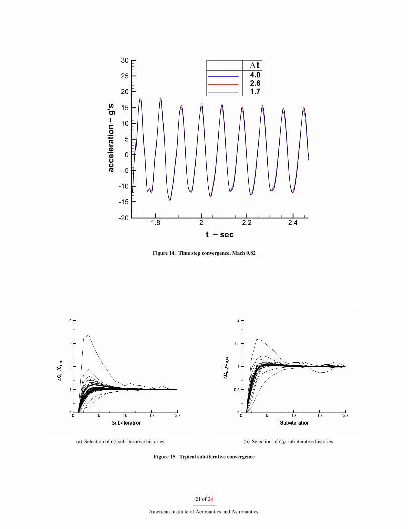
Unsteady aeroelastic simulations have been performed with the Navier-Stokes code FUN3D. The solutions are com-puted using the linear modes created by the process discussed in a previous section of this paper. The structuraldamping has been set to g = 0.02 (or damping ratio ζ = 0.01). All of the conditions simulated here are at zero degreesangle of attack. Before discussing the flutter and LCO behaviors of the SUGAR TBW, a study of the time step size,CFL number, and number of iterations necessary for accurate solutions was performed. Figure 14 shows the devel-oping LCO for a condition at Mach 0.82. Three nondimensional time step sizes (4.0,2.6,1.7) were used to assessconvergence. Each successive time step is a factor of 0.65 the previous time step size. The number of time steps perthird mode cycle are shown in Table 4. Based on the LCO amplitudes seen in Figure 14, it is clear that the smallesttime step is very near the converged LCO amplitude. The flow field CFL number used is 75, and the turbulence CFLnumber is 50, with 17−20 subiterations per time step. Figure 15 presents a random sampling of 100 lift and momentcoefficient subiteration histories. The values plotted are actually (ξn − ξ1)/(ξ20 − ξ1) for the nth subiteration withξ = (CL,CM). The lift and moment coefficients are typically quite well converged in that range of subiterations. Theseresults give confidence that the results presented here are well converged for the current grid. Note that at this time, aspatial grid convergence study has not been conducted.
The computing procedure is that steady state rigid solutions are obtained, then static aeroelastic converged solu-tions are computed with a prescribed structural damping ratio set at ζ = 0.999. The time-accurate aeroelastic solution,with the correct structural damping, is commenced by giving all 16 modes an initial modal velocity. The solutionswere continued until it was clear that an absolutely unstable solution, or a steady state LCO amplitude, or zero LCO
6 of 24
American Institute of Aeronautics and Astronautics
amplitude was evolving. Many solutions required over 20-30 cycles of LCO oscillation, to reach a converged ampli-tude.
Figure 12 presents a summary of the conditions that were simulated with FUN3D. The open symbols identifystable conditions (no LCO). Many of the closed symbols represent cases that reached an LCO. Only five conditionswere approaching what appeared to be an absolute instability, namely the three conditions (with closed symbols) atMach number 0.86 and two at Mach 0.90. Two important observations can be made from this figure. First, it is clearthat FUN3D is producing predominantly LCO’s rather than flutter. The predominance of LCO is consistent with thebehavior of the model in the wind-tunnel, which saw very few cases that were flutter. In many cases the wind tunnelproduced moderate to large LCO amplitudes. Because the structural model in FUN3D is linear, the LCO is producedentirely by nonlinear aerodynamics. The second observation is that the LCO onset dynamic pressures in the FUN3Dsimulations for Mach numbers between 0.75 and 0.80 are much closer to the experimental onset than the MSC.Nastranflutter onset. The wind-tunnel data, with the model at α =±1 degree, show a sharp rise in the onset dynamic pressurejust above Mach 0.80. The Navier-Stokes simulations, with the model at α = 0 degree, produce a slight dip in thedynamic pressure at LCO onset at Mach 0.82, then a sharp increase above that Mach number. The wind-tunnel testdid not produce flutter above Mach number 0.80, mainly because of the difficulty in traversing the flutter/LCO dip atthe higher dynamic pressures at which it would have occured.
How close are the simulated LCO amplitudes to the experimental LCO amplitudes? As seen in Figure 12, in theMach number range 0.70−0.74, the FUN3D LCO estimated onset line is significantly below even the wind tunnel testweak LCO range, but is relatively near the test weak LCO range at Mach 0.78. The maximum peak Z-accelerationsfrom the selected wind-tunnel conditions in Tables 2 and 3 can be compared with the simulation data in Table 5.Consistent with the lower onset dynamic pressures in the Mach 0.70−0.75 range, the computed LCO amplitudes tendto be larger than the amplitudes observed in the wind-tunnel test. In the Mach number range 0.78−0.80, the computedamplitudes are similar to the experimental LCO amplitudes. This can be verified in Figure 13 and Tables 2, 3 and 5.
The test point number 3443 in Table 3 is a condition that had a burst of LCO with amplitude very similar to thatcomputed by FUN3D. The experimental Mach number is 0.786 and the dynamic pressure is 97.7 psf. The wind-tunnelmodel forward wing tip Z-acceleration experienced a large amplitude burst, as seen in the time history in Figure 16.At the time of the burst, the by-pass valve was opened to protect the model. This accounts for the rapid drop in LCOamplitude. One telling feature of the LCO in this figure is the change in frequency content before and after the by-pass valve was opened. Before the opening, the oscillation occurs at a well defined frequency at about 10 Hz. Afterthe by-pass valve opening, and the amplitude drops considerably but there is a broad frequency spectrum of modeloscillation. The broad spectrum oscillation and its amplitude is indicative of model response to tunnel turbulence. Thetime range 0−1 second, over which the highest LCO amplitude occurs in Figure 16, is compared with the computedtime history of wing tip acceleration. That comparison is shown in Figure 17. The computational results were obtainedat a Mach number of 0.78 and dynamic pressure of 90 psf. The computed LCO amplitudes compare very favorablywith the experimental data in that figure. Note that what appears to be a phase shift between the two results is due tothe different predicted frequency than that of the experimental data. The dominant LCO frequency in the simulatedresults is higher than that of the experiment. This can also be seen in the spectral transform data in Figure 18. Thisaspect of the simulations is currently not well understood. Additional simulations with finer grids and/or an updatedstructural model may be required to fully assess the accuracy of the simulations.
The computed LCO onset above Mach 0.80 reveals an interesting feature that can be observed in Figure 12 andin Figures 19-21. After the slight rise in onset dynamic pressure through the Mach 0.75-0.80 range, there is a mildLCO onset at Mach 0.82. See Figure 19. By observing the time histories in Figure 20, it can be seen that while LCOonset at Mach 0.86 occurs at a slightly higher dynamic pressure, instability grows more rapidly at that Mach number.The LCO onset at Mach 0.90, between 100-115 psf, is much higher than at lower Mach numbers. Mach 0.90 and 130psf also reveals the explosive LCO amplitude growth seen at Mach 0.86. The simulations at Mach 0.86, 115 psf andMach 0.90, 130 psf were terminated with negative volumes. Accelerations at the end of the simulations were 80-110g’s and growing.
V. Concluding Remarks
This paper has focused on the simulation of the flutter and limit cycle oscillation of the Boeing Subsonic UltraGreen Aircraft Research truss-braced wing wind-tunnel model. Modeling issues and their solution related to thetransfer of the truss-braced wing wind-tunnel beam and pod finite element structural mode shapes to the CFD surfacehave been discussed. The SUGAR TBW model is a challenge because of the complex interconnection of multiplyoriented beams. Existing methods for transfer of beam deflections to CFD surface meshes have been found to be of
7 of 24
American Institute of Aeronautics and Astronautics
limited use. An alternate method of transfering modal deflections from the finite element model to the CFD surfacemesh has been developed.
The computed flutter and LCO at model angle of attack of 0 degrees have been compared with data from a recentwind-tunnel test of the Boeing Subsonic Ultra Green Aircraft Research truss-braced wing wind-tunnel model at theNASA Langley Research Center Transonic Dynamics Tunnel. The wind-tunnel test and model are discussed. Thewind tunnel model test data is for angle of attack of ±1 degrees. The high fidelity Navier-Stokes LCO simulationshave also been compared to linear flutter onset. It is found that the linear analysis predicts flutter onset dynamicpressure well below the wind-tunnel test LCO onset. Furthermore, the majority of the wind-tunnel test high dynamicscases were wing and nacelle LCO. The Navier-Stokes simulations generally also exhibit LCO rather than hard flutter.Both the linear and Navier-Stokes simulations correctly predict that the LCO is produced by a coalescence of the thirdand fourth structural modes. There is a transonic dip and then sharp rise in the wind-tunnel test LCO onset in the Mach0.78-0.80 region. Wind-tunnel conditions above that Mach number exhibited no aeroelastic instability at the dynamicpressures reached in the tunnel. The linear analysis does not show this rise. The Navier-Stokes simulations show aslight dip in LCO onset at Mach 0.82 then a sharp rise at higher Mach numbers. At Mach 0.90, the simulations weredamped at 100 psf and below. An interesting feature of the Navier-Stokes simulations is the mild LCO onset at Mach0.82, but a more explosive LCO onset at Mach 0.86 and 0.90.
There are many questions that remain unanswered from the wind-tunnel test and the computations. The physicalmechanism for the appearance of torsional modes at Mach 0.76 and +1 degree angle of attack and not at otherconditions remains unclear. Additional work is required to determine the physical mechanism causing the differencein LCO onset seen in the computations in the Mach number range 0.82− 0.90. The wind-tunnel data exhibit anangle of attack dependency, indeed, the shape of the transonic LCO onset envelop may be angle of attack dependent.Previously published flutter analyses using linear aerodynamics and nonlinear structural mode shapes show the similarangle of attack dependency as the wind-tunnel data. The present Navier-Stokes simulations have been computed atzero degree angle of attack. Future high fidelity simulations are needed to asses how LCO/flutter onset is influenced byangle of attack. The influence of structural nonlinearity, in particular in-plane strut loading on flutter/LCO onset hasnot been investigated with the high fidelity CFD code. Finally, an investigation of the influence of CFD grid resolutionand a repeat of the present computations using the version 20 FEM, that may have an improved GVT correlation, iswarranted.
References1Bradley, M. K. and Droney, C. K., “Subsonic Ultra Green Aircraft Research: Truss Braced Wing Design Exploration,” Contractor report,
The Boeing Company, June 2014.2Bradley, M. K., Droney, C. K., and Allen, T. J., “Subsonic Ultra Green Aircraft Research: Truss Braced Wing Aeroelastic Test Report,”
Contractor report, The Boeing Company, June 2014.3Coggin, J. M., Kapania, R. K., Zhao, W., Schetz, J. A., Hodigere-Siddaramaiah, V., Allen, T. J., and Sexton, B. W., “Nonlinear Aeroelastic
Analysis of a Truss Braced Wing Aircraft,” 55th AIAA/ASMe/ASCE/AHS/SC Structures, Structural Dynamics, and Materials Conference, No.AIAA-2014-0335, National Harbor, MD, Jan. 2014.
4Staff of the Aeroelasticity Branch, “The Langley Transonic Dynamics Tunnel,” Langley Working Paper LWP-799, Sept. 1969.5Corliss, J. M. and Cole, S. R., “Heavy Gas Conversion of the NASA Langley Transonic Dynamics Tunnel,” Proceedings of the 20th Advanced
Measurements and Ground Testing Technology Conference, No. 98-2710, Albuquerque, NM, June 1998.6Cole, S. R. and Rivera Jr, J. A., “The New Heavy Gas Testing Capability in the NASA Langley Transonic Dynamics Tunnel,” Royal
Aeronautical Society Wind Tunnels and Wind Tunnel Test Techniques Forum, No. 4, Cambridge, UK, April 1997.7Parlette, E. and Garriz, J., “VGRID: Unstructured Grid Generation Program Version 3.9 User’s Guide,” ViGYAN, Inc., Hampton, VA, 2007.8NASA LaRC, Hampton, VA, FUN3D Manual, Nov. 2008.9Biedron, R. T. and Thomas, J. L., “Recent Enhancements To The FUN3D Flow Solver For Moving-Mesh Applications,” 47th AIAA
Aerospace Sciences Meeting, No. 1360, 2009.10Pidaparti, R. M., “Structural and Aerodynamic Data Transformation Using Inverse Isoparametric Mapping,” Journal of Aircraft, Vol. 29,
No. 3, 1992, pp. 507–509.11Garcia:2005, “NumericalInvestigationofNonlinearAeroelasticEffectsonFlexibleHighAspectRatioWings,” Journal of Aircraft, Vol. 42, No. 4,
2005, pp. 1025–1035.12Franke, R., “Scattered Data Interpolation: Tests of Some Methods,” Mathematics of Computation, Vol. 38, No. 157, 1982, pp. 181–200.13Samareh, J. A., “Discrete Data Transfer Technique for Fluid-Structure Interaction,” 18th AIAA Computational Fluid Dynamics Conference,
No. AIAA-2007-4309, Miami, Florida, June 2007.14Farhat, C., Lesoinne, M., and LeTallec, P., “Load and Motion Transfer Algorithms for Fluid/Structure Interaction Problems with Non-
Matching Discrete Interface: Momentum and Energy Conservation, Optimal Discretization and Application to Aeroelasticity,” Computer Methodsand Applied Mechanical Engineering, Vol. 157, No. 1, 1998, pp. 95–114.
15Harder, R. L. and Desmarais, R. N., “Interpolation Using Surface Splines,” AIAA Journal, Vol. 9, No. 2, 1972, pp. 189–191.16Brown, S. A., “Displacement Extrapolations for CFD+CSM Aeroelastic Analysis,” No. AIAA-2097-1090.
8 of 24
American Institute of Aeronautics and Astronautics
17Hallissy, B. P. and Cesnik, C. E. S., “High-fidelity Aeroelastic Analysis of Very Flexible Structures,” 52nd AIAA/ASMe/ASCE/AHS/SCStructures, Structural Dynamics, and Materials Conference, No. AIAA-2011-1914, Denver, CO, April 2011.
18Palacios, R. and Cesnik, C. E. S., “Static Nonlinear Aeroelasticity of Flexible Slender Wings in Compressible Flow,” 45thAIAA/ASMe/ASCE/AHS/SC Structures, Structural Dynamics, and Materials Conference, No. AIAA-2005-1945, Austin, TX, April 2005.
19Abras, J., Lynch, C. E., and Smith, M., “Advances In Rotorcraft Simulations With Unstructured CFD,” Proceedings of the American Heli-copter Society 63rd Annual Forum, Virginia Beach, VA, 2007.
20Thepvongs, S., Cook, J. R., Cesnik, C. E. S., and Smith, M. J., “Computational Aeroelasticity of Rotating Wings with Deformable Airfoils,”Proceedings of the American Helicopter Society 65rd Annual Forum, Grapevine, TX, 2009.
9 of 24
American Institute of Aeronautics and Astronautics
Table 1. Modal data
Mode Number Frequency, Hz Description Modal Assurance Criteria