113 TERRÆ DIDATICA 13-2,2017 ISSN 1679-2300 Terræ Didatica Introduction Computer Aided Design (CAD) is the use of computer systems to assist in creation, modification and analysis of technical drawing. CAD software offers multiple capabilities for defining the geo- metrical parameters and constraints that determine the shape, dimensions, and angular relationships of the modeling entities. It constitutes an essential tool extensively used in a wide range of fields that require accurate and versatile 2D and 3D design- ing. Engineering drawing, industrial designing and all type of building projecting are actually among its main areas of application. The mentioned fea- tures indicate that CAD has an enormous potential for being applied in geological structural analysis; however, this type of application has not yet been sufficiently explored, as shown by the scarcity of updated specific references. As structural analysis is largely based on Euclid- ean geometry axioms, its conventional methods make use of descriptive geometry principles along with trigonometric functions, in combination with Mongean, stereographic, and orthographic projec- tions (Weijermars 1997, Groshong 2006). Accord- ing to this classic approach, structural problems are studied and solved by using 2D sections that, together with geological maps, represent 3D situ- ations, either with hand-made drawings or com- puter programs (Kozniewski & Orlowski 2011). However, the obtained solutions sometimes chal- lenge students’ ability to think in 3D, making the analyzed situation hard to understand. Three-dimensional visualization of natural patterns is essential for proper understanding of geological structures. Using CAD software to cre- ate 3D models of geological situations enhances the comprehension of structural problems and provides precise solutions. With this approach, the structural parameters could be obtained through direct measurements avoiding calculations and simplifying the geometrical analysis. Users currently have access to a selection of CAD commercial and open-source software. To develop the present article, AutoCAD from Autodesk has been chosen, as it is one of the most widely used CAD programs, which has been continu- ously improved since its introduction in 1982. The program is available for Windows and Mac OS platforms and, in addition, Autodesk offers free access for students, teachers, and schools to the same AutoCAD software that is used by profession- als. For this work we used the 2016 M.48.M.555 version; however, the methods are also valid for other recent versions. ARTIGO ABSTRACT: The three-dimensional (3D) modeling environment of AutoCAD is used to represent and solve problems of structural geology. As an alternative to bi-dimensional (2D) techniques of classical structural analysis, the 3D capabilities of the software are used for modeling, positioning and measuring geological structures. To introduce the proposed method, two practical examples are presented as exercises with detailed instructions. The technique consists in precisely representing the geometrical entities that comprise the geological problem within three-dimensional space to enable the direct measurement of structural parameters. Accurate results, such as fault displace- ment and the attitude of several structures, are obtained with the dimension tools of the program, so no calculations are required. Diverse 3D viewing perspectives can be adopted to enhance the comprehension of the analyzed situation. DESENHO GEOLÓGICO ASSISTIDO POR COMPUTADOR: AUTOCAD® APLICADO À GEOLOGIA ESTRUTURAL Manuscrito: Recebido:16/12/2016 Corrigido: 14/03/2017 Aceito: 01/08/2017 Citation: Chiozza S.�. 2017. Computer aided geo- Chiozza S.�. 2017. Computer aided geo- logical design: AutoCAD ® applications in structural geology. Terræ Didatica, 13(2):113-122. <http:// www.ige.unicamp.br/terraedidatica/>. Keywords: AutoCAD, structural analysis, three- dimensional modeling, fault slip, three-point problem. Computer aided geological design: AutoCAD ® applications in structural geology Univ. Fed. Ceará, UFC, Campus do Pici, Bl. 912, 60440-554 Fortaleza CE SEBASTIÁN GONZÁLEZ CHIOZZA DOI - 10.20396/td.v13i2.8650087
Transcript
113TERRÆ DIDATICA 13-2,2017 ISSN 1679-2300
TerræDidatica
IntroductionComputer Aided Design (CAD) is the use of
computer systems to assist in creation, modification and analysis of technical drawing. CAD software offers multiple capabilities for defining the geo-metrical parameters and constraints that determine the shape, dimensions, and angular relationships of the modeling entities. It constitutes an essential tool extensively used in a wide range of fields that require accurate and versatile 2D and 3D design-ing. Engineering drawing, industrial designing and all type of building projecting are actually among its main areas of application. The mentioned fea-tures indicate that CAD has an enormous potential for being applied in geological structural analysis; however, this type of application has not yet been sufficiently explored, as shown by the scarcity of updated specific references.
As structural analysis is largely based on Euclid-ean geometry axioms, its conventional methods make use of descriptive geometry principles along with trigonometric functions, in combination with Mongean, stereographic, and orthographic projec-tions (Weijermars 1997, Groshong 2006). Accord-ing to this classic approach, structural problems are studied and solved by using 2D sections that, together with geological maps, represent 3D situ-
ations, either with hand-made drawings or com-puter programs (Kozniewski & Orlowski 2011). However, the obtained solutions sometimes chal-lenge students’ ability to think in 3D, making the analyzed situation hard to understand.
Three-dimensional visualization of natural patterns is essential for proper understanding of geological structures. Using CAD software to cre-ate 3D models of geological situations enhances the comprehension of structural problems and provides precise solutions. With this approach, the structural parameters could be obtained through direct measurements avoiding calculations and simplifying the geometrical analysis.
Users currently have access to a selection of CAD commercial and open-source software. To develop the present article, AutoCAD from Autodesk has been chosen, as it is one of the most widely used CAD programs, which has been continu-ously improved since its introduction in 1982. The program is available for Windows and Mac OS platforms and, in addition, Autodesk offers free access for students, teachers, and schools to the same AutoCAD software that is used by profession-als. For this work we used the 2016 M.48.M.555 version; however, the methods are also valid for other recent versions.
ARTIGO
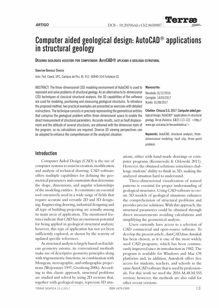
ABSTRACT: The three-dimensional (3D) modeling environment of AutoCAD is used to represent and solve problems of structural geology. As an alternative to bi-dimensional (2D) techniques of classical structural analysis, the 3D capabilities of the software are used for modeling, positioning and measuring geological structures. To introduce the proposed method, two practical examples are presented as exercises with detailed instructions. The technique consists in precisely representing the geometrical entities that comprise the geological problem within three-dimensional space to enable the direct measurement of structural parameters. Accurate results, such as fault displace-ment and the attitude of several structures, are obtained with the dimension tools of the program, so no calculations are required. Diverse 3D viewing perspectives can be adopted to enhance the comprehension of the analyzed situation.
Desenho geológico assistiDo por computaDor: autocaD® aplicaDo à geologia estrutural
Computer aided geological design: AutoCAD® applications in structural geology
Univ. Fed. Ceará, UFC, Campus do Pici, Bl. 912, 60440-554 Fortaleza CE
sebastián gonzález chiozza
DOI - 10.20396/td.v13i2.8650087
114 TERRÆ DIDATICA 13-2,2017ISSN 1679-2300
There are three basic methods to begin a com-mand: 1) typing in the command on the com-mand line, 2) selecting the command from the drop-down cascading menus or ribbon tabs, and 3) using the toolbar icon to activate the command. In this article we provide the command name that should be typed on the command line; neverthe-less, the user can choose any other method to run the commands. The search tool in the HELP menu is extremely useful to find the different possible paths to execute the desired command.
Whenever confirmation or ending of an opera-tion is required, it will be indicated with [CON-FIRM] or [ESC], respectively.
An initial knowledge of AutoCAD basic func-tions (such as zooming, panning, creating and activating layers, selecting objects, moving, erasing, copying and pasting etc.) is assumed. Extended information on these operations is available from online support provided by AutoCAD and at dif-ferent step-by-step instruction manuals with easy to understand explanations (e.g. Gindis 2013).
The different commands of the program are grouped in the “Drafting” and “Modeling” tool sets, which allow one to create, modify and manip-ulate objects in 2D and 3D.
The Properties Inspector, a palette that dis-plays the properties of the selected object or set of objects, can be opened from the drop-down Tools menu. Apart from examining the object’s param-eters, within this menu one can specify a new value to modify any property.
Technical geological drawing requires funda-mental objects to be manipulated, dimensioned and connected to each other by using specific locations (snapping points), such as midpoints, endpoints or intersections. Within AutoCAD, the Object Snap (OSNAP) tools are essential for specifying these precise locations on objects. The particular snap-ping points that will enable the accurate connec-tions required on this article are midpoint, endpoint, intersection, nearest and perpendicular. Another helpful accuracy tool that can be used to impose constraints upon line tracing is the ORTHO mode, which allows you to draw perfectly straight vertical or horizontal lines.
For adding simple labels, the DTEXT com-mand is an adequate tool. When it is activated, the following specifications will be required in sequence: starting point (just click on the desired position), text height (specify value in suitable drawing units), rotation angle (90° for horizontal
Although a variety of powerful 3D modeling software is largely available for specific geological applications in oil and gas fields (e.g. Tahmasebi et al. 2012), groundwater and ore deposits (e.g. Faure et al. 2011, Fallara et al. 2006), it is often expensive and very specific, thus becoming a restricted access resource rather than an open tool for general use.
This paper presents two hypothetical problems which are solved by applying several methods for representing, measuring and analyzing the geom-etry of geological structures in CAD environment.
Although CAD software has already been used to solve similar situations, as exposed by Jacobson (2001) and Carneiro & Carvalho (2012), the meth-ods proposed by these authors are not developed in three-dimensional space, as they just reproduce the traditional 2D solutions in the CAD drafting environment. In this work, a 3D modeling approach is used to solve the proposed problems, aiming to show AutoCAD commands and functions that are geologically useful. The detailed methods should enable the user to discover alternative ways to achieve the same results, as well as to create and solve other structural problems. The main objec-tive is to outline how structural elements could be represented, combined and dimensioned within the CAD tridimensional space. Far from exhausting the subject, this article intends to show AutoCAD’s potential as a tool for structural analysis either in the research and educational fields.
AutoCAD® for geological designThe AutoCAD software includes a diversity
of drafting and modeling tools, which can be used under various drawing modes. When used for geological drawing, some particular properties and functions are remarkably useful, so they are briefly outlined in this section.
Commands and functions of general useOn CAD environment, geological entities such
as litologies, structures, contour lines, contacts, labels, symbols and field data may be displayed on different layers, which can be turned on and off independently by using the layers palette. This property is particularly useful when working with structural analysis, as geological objects could be easily handled, being enabled or disabled for visu-alization and edition, facilitating the execution of several operations.
115TERRÆ DIDATICA 13-2,2017 ISSN 1679-2300
text) and text content. To finish, click anywhere out of the text and then press “esc”. After being created, text objects may be easily repositioned by using the grips (small blue boxes that are showed on selected objects and may be used to perform basic edition tasks).
Starting configurationsSome initial configurations that prepare the
CAD working environment for representing geo-logical situations are described in this section.
is set according to the mathematical convention (0° along the positive X axis and values increasing coun-terclockwise), the settings could be adapted to geo-logical needs. Running the DDUNITS command would open the drawing units box. To represent structural directions with the standard geological quadrant notation, the SURVEYOR option should be selected for the angle type. On the other hand, if azimuths are going to be used, the selected type shall be DECIMAL DEGREE, with the CLOCK-WISE mode activated (check box marked) and the base angle direction set to NORTH. In this paper azimuthal notation will be used.
Coordinate system To define the position of objects, AutoCAD uses
a fixed Cartesian reference system called “World Coordinate System” (WCS), in which the X axis is oriented east-west, Y is north-south and Z is vertical. The WCS constitutes a suitable frame for using UTM positioning, where easting and north-ing are equivalent to the X and Y directions and the Z coordinate being used to represent elevations. Large coordinate values should be avoided because they may interfere with certain functions of the program; it is thus convenient to use kilometers rather than meters as distance units when work-ing with UTM system. Geographic coordinates (latitude and longitude in angular values) are not supported by AutoCAD.
When necessary, the program allows creation of a User defined Coordinate System (UCS), which permits a temporary redefinition of the X, Y and Z-axes’ position and orientation. The current coor-dinate system could be visualized under the “view cube” (on the upper right corner of the drawing
area), and the coordinate values of the pointer are exhibited at the lower right corner.
LayersAs part of the initial preparation work, it is rec-
ommended to anticipate the creation of the various layers that will be required to solve the problem. Use the layers palette to perform this operation, as well as to label and attribute a different color to each layer. The suggested layers are indicated at the begging of each problem.
Geological structural problemsTwo structural problems are proposed and
solved through alternative modeling methods taking advantage of AutoCAD’s 3D resources and tools. The first situation deals with fault slip determination based on simple geological data; the solution to a similar situation using traditional methods was presented by Rowland et al. (2007). On the second problem, an original solution for the three-point geological problem is developed. The 3D modeling technique presented here repre-sents an alternative to the classical bi-dimensional graphical approaches (Ragan 2009, Carneiro & Carvalho 2012) and to calculation based method-ologies, such as the spreadsheet program devel-oped by Martinez-Torres et al. (2012).
Within the following instructions, the com-mands are indicated with capital letters, such the way as they should be typed in the command line. Whenever specific modes, views or settings should be adopted (VIEW – OSNAP MODE – POLAR TRACKING – ACTIVE LAYERS – ORTHO MODE), will be indicated between brackets in the appropriated position within the text. Names of keys, layers and specific denominations used by AutoCAD (e.g. endpoint, NW isometric etc.) will be given in italics.
Instructions have been sequentially numbered using # symbol in order to facilitate internal refer-ences within the article. At the beginning of a new instruction remember to check that unnecessary accuracy tools (OSNAP, ORTHO) are disabled to avoid computations that may interfere with the task.
The reader may notice that, in certain proce-dures, the fastest or most efficient solving methods have not been adopted; this has been done inten-tionally, in order to introduce different program capabilities.
116 TERRÆ DIDATICA 13-2,2017ISSN 1679-2300
an angle of 30° from the western side of the plane towards SE (figure 3). [CURRENT LAYER: slip] [OSNAP: nearest + endpoint] Run the LINE com-mand and select a starting point within the western side of the FP close to the NW corner; then draw a line extended up to the SW corner [CONFIRM]. Select the segment and activate the ROTATE com-mand; specify the northern endpoint as base point for rotation and type -30° (negative value to per-form a counterclockwise rotation) [CONFIRM]. Before long, this vector will create corresponding tie-points where it intersects the dike planes.
(#A2) Fault Plane (FP) positioning.
[OSNAP: nearest] To incline the plane at its dipping angle select the FP and the SL; then adopt a 3D perspective view (e.g. SW isometric) and start the 3DROTATE command. For the rotation base point, use any point at the west side of the plane; then, when prompted for a rotation axis use the 3D rotation gizmo to select the Y-axis by clicking once on the Y-axis handle (i.e. green circle which is perpendicular to the Y axis). To complete the operation, enter the dip value (40) [CONFIRM].
Then you can orient the plane according to its strike; first return to the planar TOP VIEW, then select the FP and the SL and immediately run the ROTATE command. Specify any base point within the surface and type -15 to produce a counterclockwise rotation that will leave the FP at its strike direction of 165°. Use the 3DORBIT tool to pan along different 3D views and making sure the SL lies within the FP.
The western side of the surface that remained horizontal at ground level (elevation = 0m) rep-resents the strike line (STL) of the FP.
Situation A – Fault slip calculation.PROBLEM: Figure 1 shows a simplified geo-
logic map containing a fault plane (165°/40°NE) and a faulted dike (050°/55°SE) with 320m of dextral strike separation. An oblique slip path along the fault plane has been inferred through the existence of slickenside lineations trending SE with a rake of 30°. The goal will be to measure the absolute slip and determine the slickensides attitude.
SOLUTION: As illustrated in figure 2, the geological situation will be reconstructed in tri-dimensional space and the slip of the fault will be obtained by direct measuring between correspond-ing tie-points. In this case, no real world coordi-nates are specified, so objects positioning in the drawing space is arbitrary. Nevertheless, angular configurations should be set to azimuthal mode.LAYERS: fault – dike – slip – attitude.
(#A1) Creating the Fault Plane (FP) including the Slickenside Lineation (SL).
[CURRENT LAYER: fault] To begin, an horizontal planar surface will be created with the PLANESURF tool. After running the command, choose any arbitrary location for the first corner, then type @800,800. This would create a quadran-gular surface of 800m x 800m that will be used as the fault plane (FP).
Before adjusting the FP with its strike and dip orientations, a segment representing the slick-enside lineation (SL) will be added to the plane. According to its rake, this segment should make
Figure 1. Geologic map for use in Problem A.
Figure 2. Fault slip complete model construction with fault slip represented on the fault plane (FP) between corresponding tie-points (circled).
117TERRÆ DIDATICA 13-2,2017 ISSN 1679-2300
(#A5) Trimming the exceeding portions of the dikes.
Start the SURFTRIM command and select the planes representing the two dikes and the fault, as objects to trim [CONFIRM]. After that, indicate the FP as the cutting surface [CONFIRM] and then use one click to cut the NE portion of the north-ern dike, that lies at the hanging-wall. Immediately click on the SW portion of the southern dike situ-ated at the footwall to trim it too [ESC] (figure 2).
[CURRENT LAYER: fault] [OSNAP: end-point] [TOP VIEW] Now that just the existent portions of the dike have been left, use the LINE command to create a line representing the hanging-wall dike trace on the FP (i.e. segment defined by the intersection between the FP and the south-eastern portion of the dike). When done, activate the TRIM command and select the dike trace that has just been drawn and the SL as objects to trim [CONFIRM]. Then eliminate the SL segment that extends beyond the dike trace. At this point, the SL segment represents the slip of the fault (figure 2); to get acquainted of its value, just open the proper-ties inspector and check the length of the SL line.
(#A6) Determining attitude of the SL.
[VIEW: SW isometric] The attitude of the SL will be obtained by developing the simple geo-metrical construction presented in figure 5. To start, duplicate the SL by copying it at the same position. To do this, select the line and click on its central grip to activate the moving / copying command; then, holding down the control key, click once more at the same point to create a copy [ESC]. Next, select the copied object and use the MOVE TO LAYER command (right button activation) to allocate it in the attitude layer. Then, make this attitude layer cur-rent and turn off all other layers. Repeat the previous step to duplicate the SL once again. Select the new copy and with the properties inspector adjust its end Z value to 0, to create the horizontal line in the trend of the lineation.
[OSNAP: endpoint + nearest] For measuring the plunge, run the UCS command and set the origin at the SE endpoint of the horizontal line. Then indicate its opposite NW endpoint to define the X-axis direc-tion and finally, mark any point on the SL to define the XY plane. Turn on the DIMANG command and click sequentially on both lines to have the plung-ing angle dimension (18,7°), as shown in figure 5.
(#A3) Dike representation.
[CURRENT LAYER: dike] [TOP VIEW] As in #A1, use the PLANESURF tool to create a square planar surface of 600m x 600m at an arbi-trary position within the free drawing space; this surface would represent the dike. To orientate the dike according to its attitude, just repeat the pro-ceedings of step #A2; in this case use the attitude of the dike (050°/55°SE). Note that this time, to orient the dike according to its strike, a clockwise rotation of 50° should be carried out.
[OSNAP: intersection + midpoint] Once the dike is positioned at its right attitude, run the MOVE command, pick the dike at the midpoint of its STL and displace it to the intersection between the SL and the STL of the fault plane.
(#A4) Strike separation.
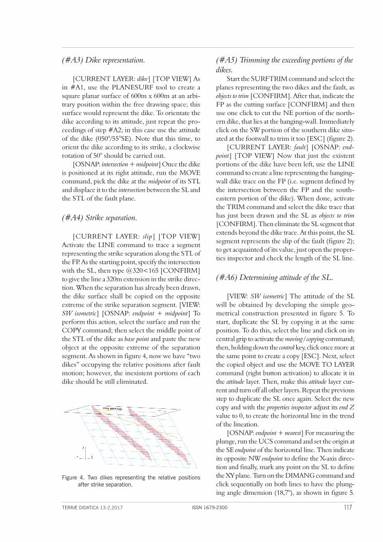
[CURRENT LAYER: slip] [TOP VIEW] Activate the LINE command to trace a segment representing the strike separation along the STL of the FP. As the starting point, specify the intersection with the SL, then type @320<165 [CONFIRM] to give the line a 320m extension in the strike direc-tion. When the separation has already been drawn, the dike surface shall be copied on the opposite extreme of the strike separation segment. [VIEW: SW isometric] [OSNAP: endpoint + midpoint] To perform this action, select the surface and run the COPY command; then select the middle point of the STL of the dike as base point and paste the new object at the opposite extreme of the separation segment. As shown in figure 4, now we have “two dikes” occupying the relative positions after fault motion; however, the inexistent portions of each dike should be still eliminated.
Figure 4. Two dikes representing the relative positions after strike separation.
118 TERRÆ DIDATICA 13-2,2017ISSN 1679-2300
structural contours that would be used to draw the contact trace on the map as shown in figure 7. To deal with this problem the topographic base map presented in figure 6 will be used as a raster image to create its georeferenced analogous version in a dwg file, with contour lines and cartographical ref-erences represented by individual CAD entities. To enhance the program’s performance, all distances as well as UTM coordinates, will be measured in kilometers. Nevertheless, contour level lines and structural contours will maintain the conventional labeling in meters.
LAYERS: references – topography – field data – structure contours – attitude – planes – contact.
(#B1) Image importing. Create an image file with figure 6 and save it
on your computer using a standard raster exten-sion, such as jpeg, png or tiff. After configuring a new drawing as specified previously, open the “layers” administration palette and create the layers sug-gested above, attributing different colors to them.
[CURRENT LAYER: 0] Use the IMAGE-ATTACH command to incorporate the image to the drawing. When placing it in the drawing area, choose any position and scale, as these parameters will be precisely adjusted in the next steps.
(#B2) Georeferencing. As the inserted map is not georeferenced
it will have to be scaled and positioned. It is convenient to start setting the scale in such a way that one drawing unit equals a kilometer, a necessary condition to achieve absolute compat-ibility with the UTM system. To do this start the
Restore the WCS by running the UCS command and typing “w” [CONFIRM].
[ORTHO] [OSNAP: nearest] [VIEW: Top] To measure the trend, first check the view cube to certify that north direction is set upright. Then use the LINE command to draw a segment in the north direction, starting at the northwestern point of the horizontal trace (figure 5). Measure the angle between the two lines by running the DIMANG tool to obtain the azimuthal trend of the slip (141,1°).
Finally, the analyzed geological situation with all its structural components can be fully appreciated by turning all the layers on and using the 3DOR-BIT command to adopt diverse 3D perspectives (figure 2).
Situation B – Contact drawing from three point geological information.
PROBLEM: The contact between two strati-form sedimentary units, a shale overlying a lime-stone, was recognized at three different outcrops situated at points A (E:538.970 - N:9671.196 - elevation:323.9), B (E:538.743 - N:9669.837 - elevation:554.1) and C (E:540.117 - N:9671.053 - elevation:754.0), within the area of the topographic map of figure 6. Assuming that the contact is a plane and has not been deformed, the objective is to use these geological data to determine the contact’s attitude and draw its cartographical trace.
SOLUTION: The three points are positioned in 3D space and a planar surface is aligned with them defining the orientation and position of the contact. Intersection lines between the inclined contact and horizontal planes are used to measure strike and dip of the contact as well as to create the
Figure 5. Three-dimensional attitude measurement of the slickenside lineation (SL).
Figure 6. Topographic base map.
119TERRÆ DIDATICA 13-2,2017 ISSN 1679-2300
(#B3) Contour line tracing. [CURRENT LAYER: topography] The contour
lines in the raster image should be reproduced as digitalized objects. The SPLINE tool is suitable to perform this action, as it can be used to draw smooth curves that pass through specified fit points. [OSNAP: nearest] Run the SPLINE command and commence marking the first point at the intersec-tion of any contour line with the border of the map. Turn off the OSNAP and continue setting fit points along the curve trajectory in order to reproduce its form with the spline. Inflection points on the curves are in general useful positions to place the fit points; if needed, use the UNDO (control + z) command to step back. If the contour line ends at the margin of the map, the [OSNAP: nearest] mode should be activated before positioning the last point; if the contour curve is a closed line, the [OSNAP: endpoint] mode will help to make it end precisely at the starting point. To finalize a line after setting its last point, hit Enter or the space bar.
nearest] To label the digitalized contour lines run the DTEXT command and mark the start point on the line to establish the position where the text shall begin. Indicate an adequate height and when prompted for the rotation angle, specify any point over the same line in the direction that text would be read. Then type the corresponding elevation value. Repeat for every line. To conclude, click anywhere out of the text and then press “esc”. To separate the texts from the lines select all the labels and, with the properties inspector opened, adjust justification to bottom left.
Now, within the topography layer, we have reproduced the original topographic map with individual objects that have specific attributes, like elevation and geographical position. These objects can be manipulated and will be used to perform further actions in combination with new geological elements that will be added.
(#B5) Data plotting. [CURRENT LAYER: field data] Run the
POINT command and type the easting, north-ing and elevation values of point A separated by a comma, then press Enter. Although the point should appear positioned as shown in figure 7, due
SCALE command and select the raster image [CONFIRM]. Then, as base point for scaling, indicate any point within the image, type “r” and [CONFIRM]. The selected option serves to give a reference of known length, such as the scale bar of the map or an object with a dimension obtained directly in the field. [ORTHO] Zoom in to gain precision, click on both extremes of the graphic scale and immediately type the value of the corresponding real distance (0.2) [CON-FIRM]. The whole map will become scaled at drawing units.
Next step is to place the map at the exact position where its UTM coordinates will match the WCS system of the drawing. To proceed, select the image, run the MOVE command and when prompted for a reference point, click precisely at the intersection of the two UTM coordinate lines. On the command line, type the known easting (E) and northing (N) coordinate values separated by a comma [CONFIRM]. The image will be displaced with the reference point being positioned at the specified coordinates and, finally, becoming completely georeferenced. Use the ZOOM to extents command to bring the map back to display.
Now the map should be transformed in an AutoCAD drawing by creating an object over every cartographical element. [CURRENT LAYER: ref-erences] [OTHO: on] The reference straight lines (i.e. north arrow, map border, coordinate lines, scale bar) could be easily traced by using the LINE command.
Figure 7. Topographic base map with data points, labeled structure contours (red) and cartographical contact trace (blue). The horizontal dip direction line (HDDL) used to define the offset distance is also shown.
120 TERRÆ DIDATICA 13-2,2017ISSN 1679-2300
0 (by default), it should be displaced vertically so as it stands at the same elevation of a contour line in the map (for example 700). To perform this, select the surface, start the MOVE command and then specify any base point. Type “@0,0,0.7” to define the relative movement in X, Y and Z directions respectively (in this case there is no displacement along X and Y directions and 0.7 kilometers up in the Z direction). Now a duplicate of the horizon-tal plane will be created and situated 0.1km above. Select the surface and run the COPY command, choose any base point within the surface and then type “@0,0,0.1”; [CONFIRM] to conclude the action and press [ESC] to exit the copying tool. Visualize at different 3D perspectives (figure 8).
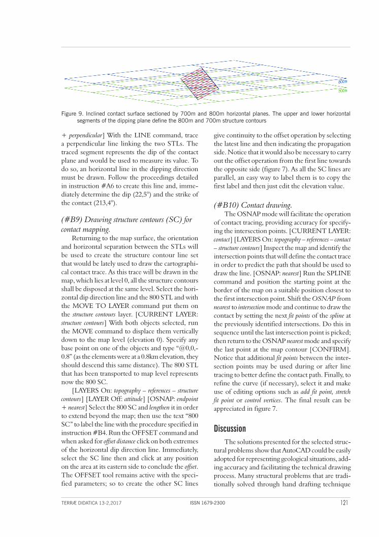
[VIEW: SE Isometric] Activate the SURFTRIM (surface trim) command and select the three planes as surfaces to trim [CONFIRM]. Immediately select both horizontal planes as cutting surfaces and finally, click on the upper and lower areas of the dipping plane to eliminate them. The intersection segments between the horizontal surfaces and the remnant dipping contact plane (figure 9), define the STLs at 700 and 800 meters that will be used to obtain the contact’s attitude and structure contours.
[OSNAP: endpoint] Activate the LINE command and draw a segment coinciding exactly with the upper horizontal intersection of the dipping plane (figure 9). Repeat for the lower intersection. Turn off all the layers except the current one (attitude). Just the two parallel STLs must have remained visible. [VIEW: SW Isometric] [OSNAP: nearest
to symbol style and size it may not be visible. This could be adjusted by using the DDPTYPE com-mand in order to define point style and dimensions. Choose a symbol different from a dot and set its size. Repeat the proceeding to plot points B and C within the map area.
(#B6) Creating the 3D positioned contact plane. An horizontal plane will be initially created and
then repositioned to fit the three points previously projected. [CURRENT LAYER: planes] [VIEW: Top] Activate the PLANESURF command to create a rectangular horizontal planar surface with its position and dimensions coincident with the base map area (see #A1 for details). [VIEW: SE isometric] [LAYERS off: references – topography] [OSNAP: endpoint + node] Run the 3DALIGN command, select the planar surface as the object to align [CONFIRM] and specify as base points, three of its vertices in sequence. To complete the action, indicate the three points A, B and C as destination points (sequentially from the lowest to the highest). The plane has now assumed the contact position; nevertheless, neither of its sides is horizontal.
(#B7) Determining contact’s strike lines (STLs). Two horizontal surfaces intercepting the
inclined contact plane will be created to define contact’s attitude and the orientation and spacing of structure contours. [CURRENT LAYER: planes] [VIEW: Top] Create a new horizontal surface by using the PLANESURF command ensuring that it wholly contains the inclined plane at the top view perspective. As the surface would be created at level
Figure 8. Frontal southwestern view of the inclined contact surface crosscutting the 700m and 800m horizontal planes. Note that the dipping plane is aligned with points A, B and C.
121TERRÆ DIDATICA 13-2,2017 ISSN 1679-2300
give continuity to the offset operation by selecting the latest line and then indicating the propagation side. Notice that it would also be necessary to carry out the offset operation from the first line towards the opposite side (figure 7). As all the SC lines are parallel, an easy way to label them is to copy the first label and then just edit the elevation value.
(#B10) Contact drawing. The OSNAP mode will facilitate the operation
of contact tracing, providing accuracy for specify-ing the intersection points. [CURRENT LAYER: contact] [LAYERS On: topography – references – contact – structure contours] Inspect the map and identify the intersection points that will define the contact trace in order to predict the path that should be used to draw the line. [OSNAP: nearest] Run the SPLINE command and position the starting point at the border of the map on a suitable position closest to the first intersection point. Shift the OSNAP from nearest to intersection mode and continue to draw the contact by setting the next fit points of the spline at the previously identified intersections. Do this in sequence until the last intersection point is picked; then return to the OSNAP nearest mode and specify the last point at the map contour [CONFIRM]. Notice that additional fit points between the inter-section points may be used during or after line tracing to better define the contact path. Finally, to refine the curve (if necessary), select it and make use of editing options such as add fit point, stretch fit point or control vertices. The final result can be appreciated in figure 7.
DiscussionThe solutions presented for the selected struc-
tural problems show that AutoCAD could be easily adopted for representing geological situations, add-ing accuracy and facilitating the technical drawing process. Many structural problems that are tradi-tionally solved through hand drafting technique
+ perpendicular] With the LINE command, trace a perpendicular line linking the two STLs. The traced segment represents the dip of the contact plane and would be used to measure its value. To do so, an horizontal line in the dipping direction must be drawn. Follow the proceedings detailed in instruction #A6 to create this line and, imme-diately determine the dip (22,5°) and the strike of the contact (213,4°).
(#B9) Drawing structure contours (SC) for contact mapping.
Returning to the map surface, the orientation and horizontal separation between the STLs will be used to create the structure contour line set that would be lately used to draw the cartographi-cal contact trace. As this trace will be drawn in the map, which lies at level 0, all the structure contours shall be disposed at the same level. Select the hori-zontal dip direction line and the 800 STL and with the MOVE TO LAYER command put them on the structure contours layer. [CURRENT LAYER: structure contours] With both objects selected, run the MOVE command to displace them vertically down to the map level (elevation 0). Specify any base point on one of the objects and type “@0,0,-0.8” (as the elements were at a 0.8km elevation, they should descend this same distance). The 800 STL that has been transported to map level represents now the 800 SC.
[LAYERS On: topography – references – structure contours] [LAYER Off: attitude] [OSNAP: endpoint + nearest] Select the 800 SC and lengthen it in order to extend beyond the map; then use the text “800 SC” to label the line with the procedure specified in instruction #B4. Run the OFFSET command and when asked for offset distance click on both extremes of the horizontal dip direction line. Immediately, select the SC line then and click at any position on the area at its eastern side to conclude the offset. The OFFSET tool remains active with the speci-fied parameters; so to create the other SC lines
Figure 9. Inclined contact surface sectioned by 700m and 800m horizontal planes. The upper and lower horizontal segments of the dipping plane define the 800m and 700m structure contours
122 TERRÆ DIDATICA 13-2,2017ISSN 1679-2300
trutural. Terrae Didatica, 8(2):83-93.Fallara F., Legault M., Rabeau O. 2006. 3-D In-
tegrated Geological Modeling in the Abitibi Subprovince (Quebec, Canada): Techniques and Applications. Exploration and Mining Geol-ogy, 15:27-41.
Faure F., Godey S., Fallara F., Trepanier S. 2011. Seismic Architecture of the Archean North American Mantle and Its Relationship to Dia-mondiferous Kimberlite Fields. Economic Geol-ogy, 106:223-240.
Gindis E. 2013. Up and Running with AutoCAD 2014. Oxford: Academic Press. 727p.
Groshong R.H. 2006. 3-D Structural Geology. A Prac-tical Guide to Quantitative Surface and Subsurface Map Interpretation (2nd ed.). Heidelberg: Springer-Verlag. 400p.
Jacobson C.E. 2001. Using AutoCAD for descriptive geometry exercises in undergraduate structural geology. Computers & Geosciences, 27(1):9-15.
Kozniewski E., Orlowski M. 2011. From 2D Mon-gean Projection to 3D model in AutoCAD. The Journal of Polish Society for Geometry and Engineer-ing Graphics, 22:49-54.
Martinez-Torres L. M., Lopetegui A., Eguiluz L. 2012. Automatic resolution of the three-points geological problem. Computers & Geosciences, 42:200-202.
Ragan D.M. 2009. Structural Geology. An Introduc-tion to Geometrical Techniques (4th ed.). New York: Cambridge University Press. 602p.
Rowland S.M., Duebendorfer E.M., Schiefelbein I.M. 2007. Structural analysis and synthesis: A labo-ratory course in Structural Geology (3rd ed). Oxford: Blackwell. 301p.
Tahmasebi P., Hezarkhani A., Sahimi M. 2012. Mul-tiple-point geostatistical modeling based on the cross-correlation functions. Computational Geo-sciences, 16:779-797.
Weijermars R. 1997. Structural geology and map in-terpretation. Amsterdam: Alboran Science Pub-lishing. 378p.
based essentially in descriptive geometry and trigo-nometry are treated in 3D space using true spatial relations and relative positions (with no specific projection required). This more realistic approach reduces the abstraction of graphical representations that involve projections (orthogonal, orthographic or stereographic). Indeed, AutoCAD has a proved potential as a structural analysis tool, as through 3D modeling, it enables geometric operations (projections, translations, measurements, etc.) that when manually performed, have limited accuracy and require more complex and time-consuming manipulations. Furthermore, an outstanding aspect of the presented methods is that no calculation is involved and the results are obtained by direct measuring.
Traditional treatment of problems throughout manual methods has great didactical value and should be not be set apart as it provides the student with concrete experiences of measuring and scale dimensioning, which in computer environment may result more difficult to capitalize. Neverthe-less, when considering didactical aspects, it should be noticed that computational 3D modeling con-tributes to construct the conception that geological structures have volume and aids in the process of learning to see beyond the outcropping surface.
AcknowledgementsThe author would like to thank the geologist
Patricio Figueredo for valuable discussions, posi-tive criticism and comments, which significantly improved this work.
Resumo: O ambiente de modelagem tridimensional (3D) do AutoCAD é utilizado para representar e resolver problemas de geologia estrutural. Como alternativa às técnicas bidimensionais (2D) da analise estrutural clássica, as capacidades 3D do software são usadas para modelar posicionar e medir estruturas geológicas. Para introduzir a metodologia proposta, são apresentados dois exemplos práticos como exercícios com instruções detalhadas. A técnica consiste em representar precisamente as entidades geológicas que compõem o problema geológico no espaço tridimensional, para poder medir diretamente os parâmetros estruturais. Resultados acurados, tais como rejeito de falha e a atitude de diversas estruturas, são obtidos com as ferramentas de medição do programa, sem necessidade de cálculos adicionais. Várias perspectivas de visualização 3D podem ser adotadas para melhorar a compreensão da situação analisada.
PALAVRAS-CHAVE: AutoCAD; análise estrutural; modelagem tridimensional; rejeito de falha; problema dos três pontos.