COMPUTER-AIDED GEOMETRIC DESIGN COMPUTER-AIDED GEOMETRIC DESIGN AND AND COMPUTER GRAPHICSCOMPUTER GRAPHICS::

HIGH LEVEL COMPUTATION PROGRAMS HIGH LEVEL COMPUTATION PROGRAMS ((MATHEMATICAMATHEMATICA AND AND MATLABMATLAB) IN CAGD ) IN CAGD

AND COMPUTER GRAPHICSAND COMPUTER GRAPHICS

Andrés Iglesiase-mail: iglesias@unican.es

Web pages: http://personales.unican.es/iglesiashttp://etsiso2.macc.unican.es/~cagd

Department of Applied Mathematics and Computational Sciences

University of Cantabria UC-CAGD UC-CAGD GroupGroup

© 2001 A

ndrés Iglesias. See: http://personales.unican.es/iglesias

Symbolic and Numerical computation programs♦ In the last few years, the extraordinary advances in hardware and software have made possible the appearance of a new generation of Scientific Computation Programs (SCPs):

• either symbolic, as Mathematica• or numerical, as Matlab

# The SCPs are easier to use, because: - they incorporate many mathematical and programming commands and libraries - their algorithms are very optimized - they have a powerful and user-friendly interface# The SCPs are very powerful, because: - their programming languages incorporate not only the procedural but also the functional programming including, in several cases, pattern recognition and object-oriented programming. - they have a very remarkable graphical capabilities.# The NCPs are very popular. Both Mathematica and Matlab are used for hundreds of thousands of industrial, government and academic users around the world.

© 2001 Andrés Iglesias. See: http://personales.unican.es/iglesias

Bernstein[i_,n_,v_]:= Binomial[n,i] (1-v)^(n-i) v^i

Mathematica for CAGD and Computer GraphicsMathematical expressions can be easily implemented in Mathematica; in most cases, this process consists of a simple translation of these expressions to its programming language.

In[3]:= Bernstein[1,3,t]Out[3]:= 3 (1-t)2 t

In[1]:= <<CAGD.m First, loading the package

In[4]:= Show[ Table[Plot[Bernstein[i,4,t], {t,0,1},PlotRange->{0,1}], {i,0,4}] ]

We have developed a Mathematica package that incorporates the mostusual curves and surfaces in CAGD and computer graphics.

( )Bn

i (t) =n

i(1 − t)n−iti

© 2001 Andrés Iglesias. See: http://personales.unican.es/iglesias

Mathematica for CAGD and Computer Graphics

In[6]:= pts={{1,1},{2,4},{3,0},{4,3},{5,-1},{6,0}};

In[7]:= BezierCurve[pts,t]Out[7]:= {1+5t, 1+15t-70t2+140t3-140t4+54t5}

We have obtained the symbolic expression for the Bézier curve !!!

In[8]:= ptos3D={{1,4,4},{2,2,3}, {3,0,3},{3,4,0},{4,5,2}};

In[9]:= PlotBezierCurve[ptos3D,t]

The same commands work for two- and three- dimensional points.

n∑

i=0PiB

ni (t)

BezierCurve[pts:{{_,_}..}|{{_,_,_}..},v_]:= Module[{n=Length[pts]-1}, Table[Bernstein[i,n,v],{i,0,n}].pts //Simplify ];

© 2001 Andrés Iglesias. See: http://personales.unican.es/iglesias

BezierSurf[pts:{{{_,_,_}..}..},{u_,v_}]:= Module[{m=Length[pts]-1,U,V, n=Length[First[pts]]-1}, {U,V}=MapThread[ Table[ Bernstein[i,#1,#2], {i,0,1}]&,{{m,n},{u,v}} ]; Plus @@ (U.pts*V) //Simplify ]

Mathematica for CAGD and Computer Graphics

The previous commands can be easily generalized to the surface case. For example:

x y z x y z x y z x y z x y z x y z0 0 1 0 1 2 0 2 3 0 3 3 0 4 2 0 5 11 0 2 1 1 3 1 2 4 1 3 4 1 4 3 1 5 22 0 3 2 1 4 2 2 5 2 3 5 2 4 4 2 5 33 0 3 3 1 4 3 2 5 3 3 5 3 4 4 3 5 34 0 2 4 1 3 4 2 4 4 3 4 4 4 3 4 5 25 0 1 5 1 2 5 2 3 5 3 3 5 4 2 5 5 1

Table of 3-dimensional control points

BEZIER SURFACES © 2001 Andrés Iglesias. See: http://personales.unican.es/iglesias

Mathematica for CAGD and Computer Graphics

In Mathematica 3.0 or higher users can easily create palettes for incorporating their own commands.

Mathematica 3.0 palettes In[]:= Bernstein[1,3,u]Out[]:= 3 (1-u)2 u

In[]:= BezierCurve[pts,t]Out[]:= {1+5t, 1+15t-70t2+140t3-140t4+54t5}

In[]:= ptos3D={{1,4,4},{2,2,3}, {3,0,3},{3,4,0},{4,5,2}};

In[]:= PlotBezierCurve[ptos3D,t]

In[]:= PlotBezierSurf[ptos3D,{u,v}]

MATHEMATICA PALETTES

© 2001 Andrés Iglesias. See: http://personales.unican.es/iglesias

Mathematica for CAGD and Computer GraphicsThe CAGD.m package can be applied for educational purposes!!!

EXAMPLE

We know that the Bézier curves hold the convex hull property: the curve lies entirely within the convex polygon determined by its control points.

In[1]: p1={{1/2,1},{2,3/2}, {3,1},{4,2},{5,1/2},{6,3}};

In[5]: Show[ {Graphics[ {RGBColor[1,1,0], Polygon[%]}],c1} ]

In[3]: <<DiscreteMath` ComputationalGeometry`

In[4]: ConvexHull[p1]; Part[p1,#]& /@ %Out[4]: {{6,3},{1/2,1},{5,1/2}}

We introduce some control points.

In[2]: c1=PlotBezierCurve[p1,t];

We take advantage of the computational geometryMathematica packages, avoiding to calculate the convex hull of the given list of points:

© 2001 Andrés Iglesias. See: http://personales.unican.es/iglesias

Mathematica for CAGD and Computer Graphics

EXAMPLE: TWO DIMENSIONAL TRANSFORMATIONS

This example shows how the previouscommands can be combined with two-dimensional transformations.

List of 22 control points

Reflection

Rotations

In[1]:= BezierCurve[spitop,t]

Out[1]: {21 t-105 t2+2992.5 t4-20349 t5++............................... , ................................+4.36432 106 t19-737383 t20+59270.5 t21}

A 21-degree polynomial !!!!

spitop={{0,16},{1,16},{1.5,16},{1.5,16},{1.5,16}, {1.5,16},{1.5,14.5},{1.5,14.5},{1.5,14.5}, {1.5,14.5},{1.5,14.5},{2,14.5},{3.5,14}, {5,13},{5.5,11},{4.5,8.5},{3,7},{1.5,6}, {1,4.5},{0.5,3},{0,1.5},{0,0}};

© 2001 Andrés Iglesias. See: http://personales.unican.es/iglesias

Mathematica for CAGD and Computer Graphics

EXAMPLE: THREE DIMENSIONAL TRANSFORMATIONS

This previous example can be extendedto the three dimensional case.

© 2001 Andrés Iglesias. See: http://personales.unican.es/iglesias

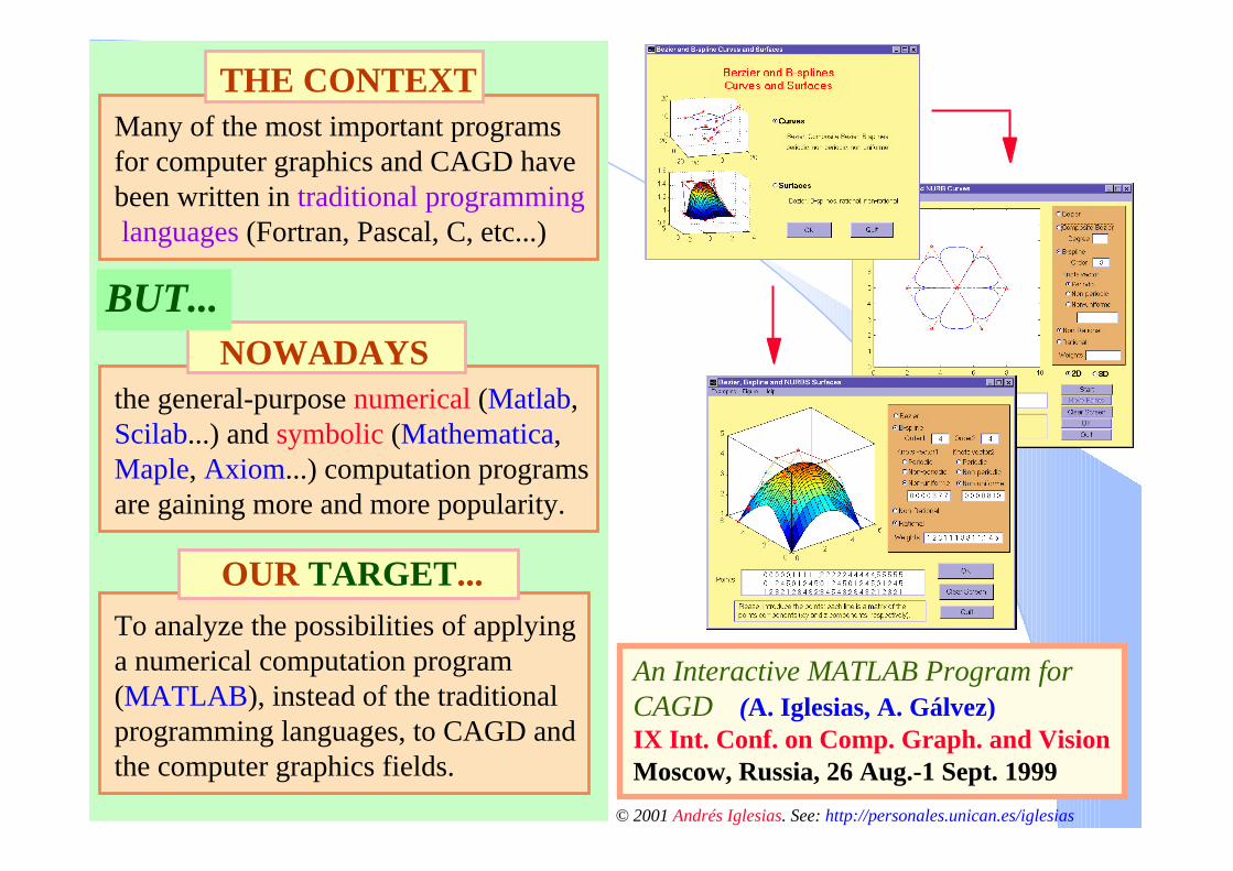
Many of the most important programs for computer graphics and CAGD have been written in traditional programming languages (Fortran, Pascal, C, etc...)

THE CONTEXT

the general-purpose numerical (Matlab,Scilab...) and symbolic (Mathematica, Maple, Axiom...) computation programs are gaining more and more popularity.

NOWADAYS

BUT...

OUR TARGET...To analyze the possibilities of applying a numerical computation program (MATLAB), instead of the traditional programming languages, to CAGD and the computer graphics fields.

An Interactive MATLAB Program for CAGD (A. Iglesias, A. Gálvez)IX Int. Conf. on Comp. Graph. and VisionMoscow, Russia, 26 Aug.-1 Sept. 1999

© 2001 Andrés Iglesias. See: http://personales.unican.es/iglesias

MATLAB

WEB PAGE: www.mathworks.com• Spreading:Spreading:

••Graphical capabilities.Graphical capabilities.

• Programming language:Programming language:

– Hundreds of thousands of users.– Industrial, academic and research environments.– Available versions for Windows 95, 98 and NT, Macintosh, UNIX, VMS, Linux, Digital, etc...

– It is based on C.– Arrays do not require dimensioning.– Incorporates functional programming.

Plotting 2D and 3D data, patches, hidden line removal, colors, lighting, reflectances, texture mapping, files management, etc...

MATLAB files External files

MATLAB

MATLAB user interface

MATLAB Kernel

Signal Control

TimeSeries

TOOLBOXES

GUIsOOP

Symbolic

MAPLE

CC

YOUR OWN TOOLBOXES

© 2001 Andrés Iglesias. See: http://personales.unican.es/iglesias

Building numerical libraries for CAGD

Implementation of an extensive set of numerical libraries for CAGD.

TASK:MATLAB incorporates:

• Basic commands for interpolation: 'nearest' - nearest neighbor 'linear' - linear 'spline' - cubic spline 'cubic' - cubic

• A Spline Toolbox by Carl de Boor. - difficult to understand - it is very limited - not so useful for industry - it lacks of many important commands in CAGD

- Bézier curves and surfaces: both rational and nonrational Bézier and composite Bézier.

- B-splines curves and surfaces: for any order and knots vector (periodic, nonperiodic, nonuniform) and weights (including NURBS).

- Two- and three-dimensional transformations.

- Projections and perspectives.

MATLAB Kernel

TOOLBOXES

© 2001 Andrés Iglesias. See: http://personales.unican.es/iglesias

An illustrative example: Bézier curves

function M = mij(n)for i=0:n for j=0:n M(i+1,j+1)=(-1)^(ji)*binom(n,j)*binom(j,i); endendM=M(1:n+1,1:n+1);

function Bezier(ptos)[n,d]=size(ptos);n=n-1;bt=ptos'*mij(n)*ti(n);if d==2plot(bt(1,:),bt(2,:),ptos(:,1),ptos(:,2),'r-.p')elseplot3(bt(1,:),bt(2,:),bt(3,:), ... ptos(:,1),ptos(:,2),ptos(:,3),'r-.p')endrotate3d

function c=binom(n,i)if i==n | i==0 c=1;elseif i<n & i>=0 c=factorial(n)/ (factorial(i)*factorial(n-i));else c=0;end

function T=ti(n) m=1;t=0:0.05:m; % step=0.05T=[];for i=0:n T= [T;t.^i];end

[ See: G. E. Farin. Curves and Surfaces for CAGD, 3rd ed., Academic Press, San Diego (1993)]

The main function: Defining the factorial and binomial function:

function f=factorial(n)if n==1 f=1;else f=n*factorial(n-1);end

Auxiliar functions:

© 2001 Andrés Iglesias. See: http://personales.unican.es/iglesias

The case of Bézier surfaces

function M = mij(n)for i=0:n for j=0:n M(i+1,j+1)=(-1)^(ji)*binom(n,j)*binom(j,i); endendM=M(1:n+1,1:n+1);

function SupBezier(ptos)[m,n,o]=size(ptos);for k=1:3b(:,:,k)=ti(m-1)'*mij(m-1)'*ptos(:,:,k)... *mij(n-1)*ti(n-1);endsurf(b(:,:,1),b(:,:,2),b(:,:,3)), hold on,mesh(ptos(:,:,1),ptos(:,:,2),ptos(:,:,3)),hidden offplot3(ptos(:,:,1),ptos(:,:,2),ptos(:,:,3),'bp')rotate3d

function c=binom(n,i)if i==n | i==0 c=1;elseif i<n & i>=0 c=factorial(n)/ (factorial(i)*factorial(n-i));else c=0;end

function T=ti(n) m=1;t=0:0.05:m; % step=0.05T=[];for i=0:n T= [T;t.^i];end

[ See: G. E. Farin. Curves and Surfaces for CAGD, 3rd ed., Academic Press, San Diego (1993)]

The main function: Defining the factorial and binomial function:

function f=factorial(n)if n==1 f=1;else f=n*factorial(n-1);end

Auxiliar functions:

© 2001 Andrés Iglesias. See: http://personales.unican.es/iglesias

Applications to industry

In an European project we propose the use of symbolic and numerical tools for CAGD in industry.

(Ref: 1FD97-0409)

Computational Algebra and Geometry Group University of Cantabria

Computer-Aided Geometric Design Group University of Cantabria

www.candemat.com

http://matsun1.matesco.unican.es/CAG/

http://etsiso2.macc.unican.es/~andres/UC-CAGD/

MATHEMATICA MATLAB

MAPLE

© 2

001

And

rés

Igle

sias

. See

: ht

tp:/

/per

sona

les.

unic

an.e

s/ig

lesi

as

Applications to industry

IGES FILECurves and surfaces

Numerical

Symbolic

1 Reading 2 Evaluation

Textures

3 Representation

4 Visualization

Lighting

Patches

Reflectance

Color

Interactivity

Wireframe

Mesh

© 2001 Andrés Iglesias. See: http://personales.unican.es/iglesias

Tasks to be done

• Build a IGES-MATLAB Converter - MATLAB file management (The formats TIFF, JPEG, BMP, PCX, XWD and HDF are available)

• Applying the CAGD MATLAB Toolbox - We shall obtain both a numerical and a graphical output

•Visualization - Taking advantage of the MATLAB graphical capabilities - Generating animations - Converting to VRML language VRMLplot by Craig Sayers www.dsl.whoi.edu/DSL/sayers/VRMLplot

VRML file WEB BROWSER Interactive Graphical Output

IGES FILE

MATLAB

© 2001 Andrés Iglesias. See: http://personales.unican.es/iglesias