55
Computer-Aided Verification of Electronic Circuits and Systems EE219A – Fall 2002 Professor: Prof. Alberto Sangiovanni-Vincentelli Instructor: Alessandra Nardi
| Date post: | 17-Dec-2015 |
| Category: |
Documents |
| Upload: | eustacia-morris |
| View: | 219 times |
| Download: | 0 times |

Computer-Aided Verification of Electronic Circuits and Systems
EE219A – Fall 2002
Professor: Prof. Alberto Sangiovanni-Vincentelli
Instructor: Alessandra Nardi
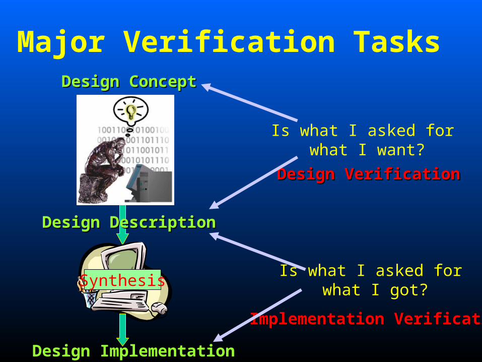
Major Verification TasksDesign ConceptDesign Concept
Design DescriptionDesign Description
Design ImplementationDesign Implementation
Synthesis
Design VerificationDesign Verification
Is what I asked for what I want?
Implementation VerificationImplementation Verification
Is what I asked for what I got?
Functional Verification
• Specification ValidationSpecification Validation: Are the specifications consistent? Are they complete, i.e. if the design satisfies them are we sure that it is correct?
• Design VerificationDesign Verification: Is the “entry” level description of my design correct? Most common reason for chip failure.
• Implementation VerificationImplementation Verification: Are the different levels of abstractions generated by the design process equivalent?
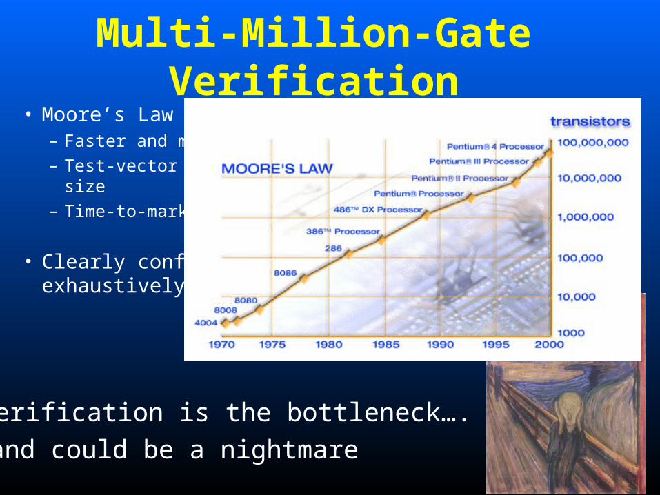
Multi-Million-Gate Verification• Moore’s Law
– Faster and more complex designs
– Test-vector size grows even faster than design size
– Time-to-market pressures will certainly not abate
• Clearly conflicts with the need to exhaustively verify a design before sign-off
Verification is the bottleneck….
….and could be a nightmare

Verification Techniques
• Simulation (FT):Simulation (FT):Build a mathematical model of the components of the design, submit test vectors and solve the equations that give the output as a function of the input and of the models on a computer
• Formal Verification (F):Formal Verification (F):Prove mathematically that:– A description has a set of properties
– Two descriptions at different levels of abstraction are functionally equivalent
Goal:Goal: Ensure the design meets its functional (F) and timing (T) requirements at each of those levels of abstraction
Verification Techniques
• Static Timing Analysis (T):Static Timing Analysis (T):Analyze circuit’s topological paths and check their timing properties and their impact on circuit delay
• Emulation (F):Emulation (F):Map the design onto the components of the emulation machine, submit test vectors and check the outputs of the machine possibly physically connecting them to a system
• Prototyping (F): Prototyping (F): Build a hardware implementation of the design and operate it
Goal:Goal: Ensure the design meets its functional (F) and timing (T) requirements at each of those levels of abstraction

Simulation: Perfomance vs Abstraction
.001x
SPICE
Event-drivenSimulator
Cycle-basedSimulator
1x 10xPerformance and Capacity
Abs
trac
tion
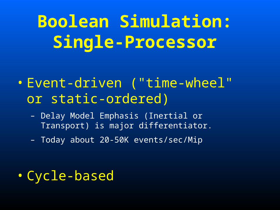
Boolean Simulation: Single-Processor
• Event-driven ("time-wheel" or static-ordered)– Delay Model Emphasis (Inertial or Transport) is major
differentiator.
– Today about 20-50K events/sec/Mip
• Cycle-based

Cycle-based simulation
• Cycle-based simulators work off of a control and data-flow representation
• Treats everything in the design description as either clocked element or zero-delay combinational logic
• Advantages– exceptionally fast– same internal representation for both simulation
and synthesis– predicted results same as synthesized logic

Cycle-based Algorithm
• Input design must be completely synchronous
• Only evaluate on the clock edge– First: evaluate all combinational logic– Next: latch values into state registers– Repeat on next clock edge
CCoommb.b.
SSttaattee
SSttaattee
LLooggiicc
clockclock

Boolean Simulation: Hardware Acceleration
• Quickturn-IBM (Cobalt) type
– 1M Event/sec.
– Requires fairly long compilation time

Emulation
• Based on re-programmable FPGA technology.
• Only functional verification (no timing verification yet).
• Close to implementation performance.
– Can boot operating system, give look and feel for final implementation.
• Allows hardware-software co-design.
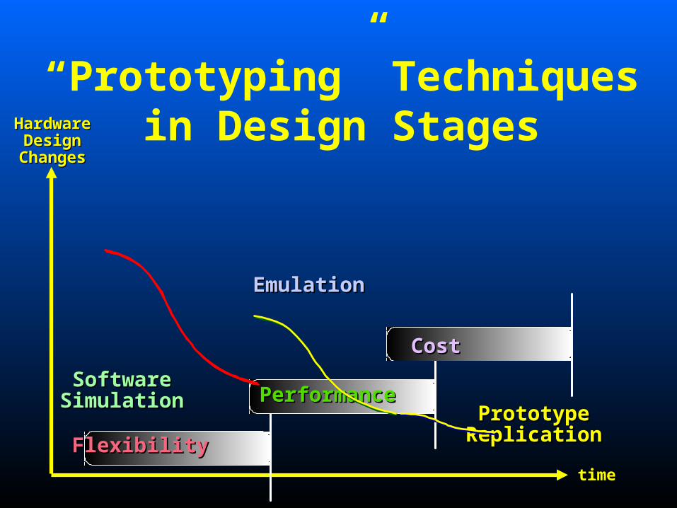
“Prototyping” Techniques in Design Stages
timetime
HardwareHardwareDesignDesignChangesChanges
SoftwareSoftwareSimulationSimulation
EmulationEmulation
PrototypePrototypeReplicationReplicationFlexibilityFlexibility
PerformancePerformance
CostCost
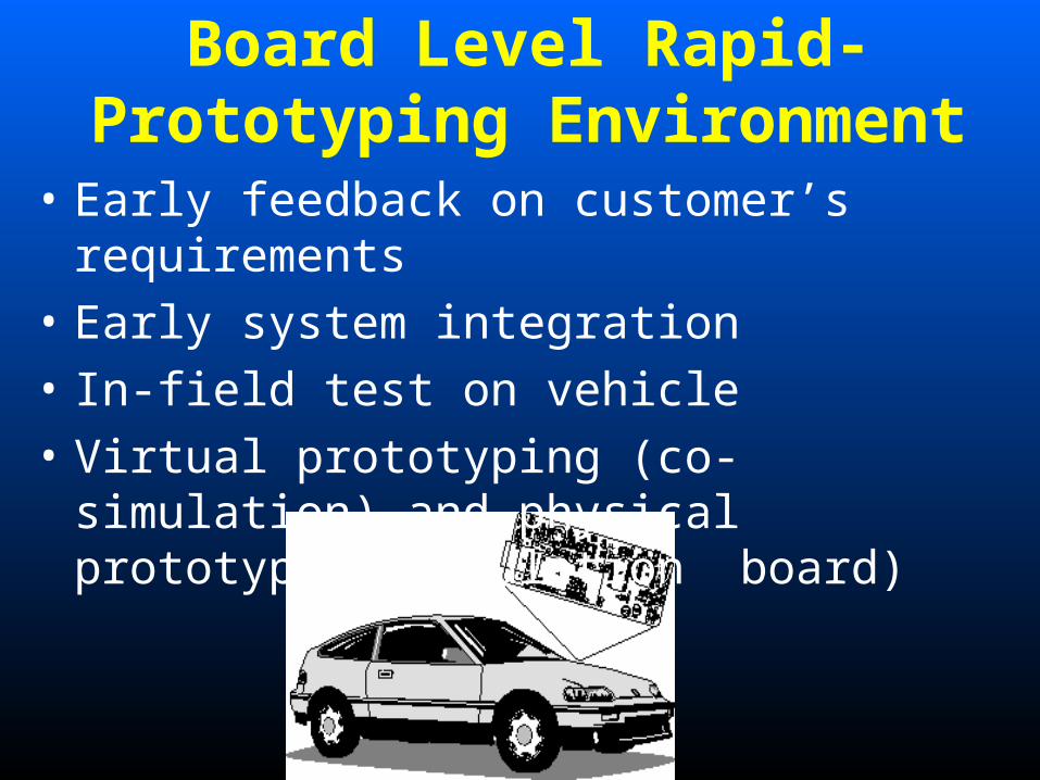
Board Level Rapid-Prototyping Environment
• Early feedback on customer’s requirements
• Early system integration
• In-field test on vehicle
• Virtual prototyping (co-simulation) and physical prototyping (emulation board)

Simulation vs Formal Methods
• Degree of confidence in simulation depends on test vectors selected by the designers
• Formal methods most important for implementation verification
• Simulation cannot be replaced by formal verification especially for design verification: specifications are often not given in rigorous terms and are not complete

Analog Circuits – A World Apart• Analog circuits’ behavior specified in terms of
complex functions: time-domain, frequency-domain, distorsion, noise, power spectra….
• Required accuracy of models much higher than digital
• …emerging paradigm: Field Programmable Analog Array for prototyping (and more)

Circuit Simulation
• Formulation of circuit equations – STA, MNA
• Solution of linear equations – LU factorization, QR factorization, Krylov
Methods
• Solution of nonlinear equations– Newton’s method
• Solution of ordinary differential equations– One-step and Multi-step methods
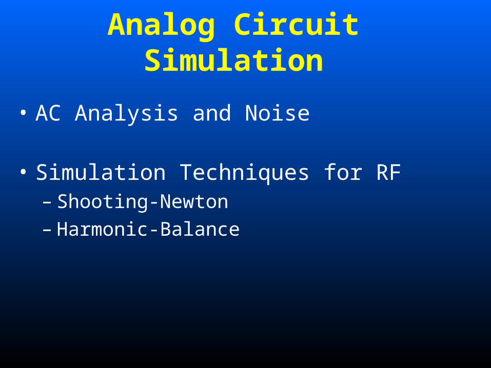
Analog Circuit Simulation
• AC Analysis and Noise
• Simulation Techniques for RF– Shooting-Newton– Harmonic-Balance
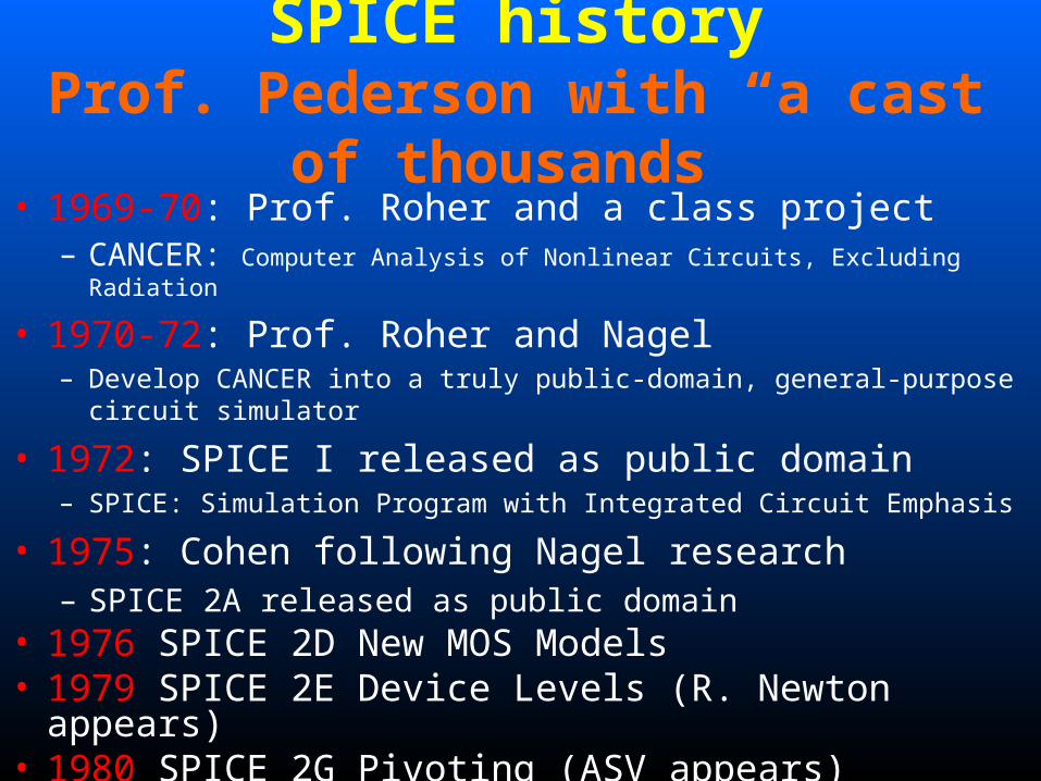
SPICE historyProf. Pederson with “a cast of
thousands”• 1969-70: Prof. Roher and a class project
– CANCER: Computer Analysis of Nonlinear Circuits, Excluding Radiation
• 1970-72: Prof. Roher and Nagel– Develop CANCER into a truly public-domain, general-purpose circuit simulator
• 1972: SPICE I released as public domain– SPICE: Simulation Program with Integrated Circuit Emphasis
• 1975: Cohen following Nagel research– SPICE 2A released as public domain
• 1976 SPICE 2D New MOS Models• 1979 SPICE 2E Device Levels (R. Newton appears)• 1980 SPICE 2G Pivoting (ASV appears)

Circuit Simulation
Simulator:Solve dx/dt=f(x) numerically
Input and setup Circuit
Output
Types of analysis:– DC Analysis– DC Transfer curves– Transient Analysis– AC Analysis, Noise, Distortion, Sensitivity

Ideal Elements: Reference Direction
Branch voltages and currents are measured according to the associated reference directions– Also define a reference node (ground)
+
_
v i
Two-terminal
+
_
v1
i1
Two-port
i1
+
_
v2
i2
i2

Branch Constitutive Equations (BCE)
Ideal elementsElement Branch Eqn
Resistor v = R·i
Capacitor i = C·dv/dt
Inductor v = L·di/dt
Voltage Source v = vs, i = ?
Current Source i = is, v = ?
VCVS vs = AV · vc, i = ?
VCCS is = GT · vc, v = ?
CCVS vs = RT · ic, i = ?
CCCS is = AI · ic, v = ?

Conservation Laws
• Determined by the topology of the circuit
• Kirchhoff’s Voltage Law (KVL): Every circuit node has a unique voltage with respect to the reference node. The voltage across a branch eb is equal to the difference between the positive and negative referenced voltages of the nodes on which it is incident
• Kirchhoff’s Current Law (KCL): The algebraic sum of all the currents flowing out of (or into) any circuit node is zero.

Nodal Analysis - ExampleR3
0
1 2
R1G2v3
R4Is5
52
1
433
32
32
10
111
111
sie
e
RRR
RG
RG
R

Spice input format: Rk N+ N- Rkvalue
Nodal Analysis – Resistor “Stamp”
kk
kk
RR
RR11
11N+ N-
N+
N-
N+
N-
iRk
sNNk
others
sNNk
others
ieeR
i
ieeR
i
1
1KCL at node N+
KCL at node N-
What if a resistor is connected to ground?
….Only contributes to the
diagonal
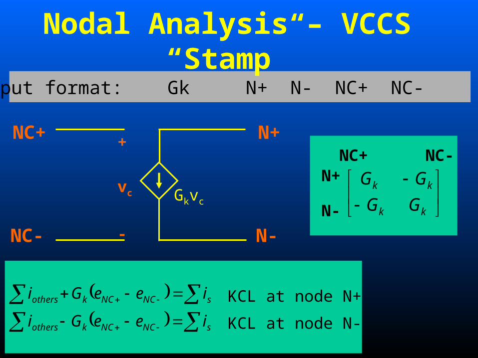
Spice input format: Gk N+ N- NC+ NC- Gkvalue
Nodal Analysis – VCCS “Stamp”
kk
kk
GG
GGNC+ NC-
N+
N-
N+
N-
Gkvc
NC+
NC-
+
vc
-
sNCNCkothers
sNCNCkothers
ieeGi
ieeGi KCL at node N+
KCL at node N-
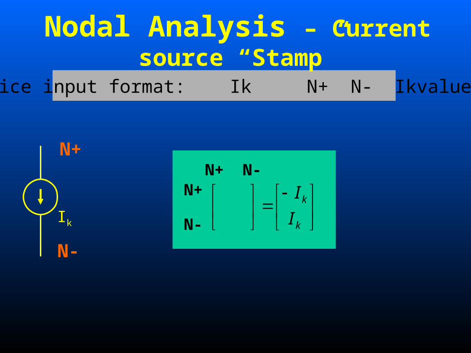
Spice input format: Ik N+ N- Ikvalue
Nodal Analysis – Current source “Stamp”
k
k
I
IN+ N-
N+
N-
N+
N-
Ik

Nodal Analysis (NA)
Advantages• Yn is often diagonally dominant and symmetric• Eqns can be assembled directly from input data• Yn has non-zero diagonal entries• Yn is sparse
Limitations• Conserved quantity must be a function of node
variable– Cannot handle floating voltage sources, VCVS, CCCS,
CCVS

Modified Nodal Analysis (MNA)
• ikl cannot be explicitly expressed in terms of node voltages it has to be added as unknown (new column)
• ek and el are not independent variables anymore a constraint has to be added (new row)
How do we deal with independent voltage sources?
ikl
k l
+ -Ekl
klkl
l
k
Ei
e
e
011
1
1k
l

MNA – Voltage Source “Stamp”
ik
N+ N-
+ -Ek
Spice input format: ESk N+ N- Ekvalue
kE
0
00 0 1
0 0 -1
1 -1 0
N+
N-
Branch k
N+ N- ik RHS
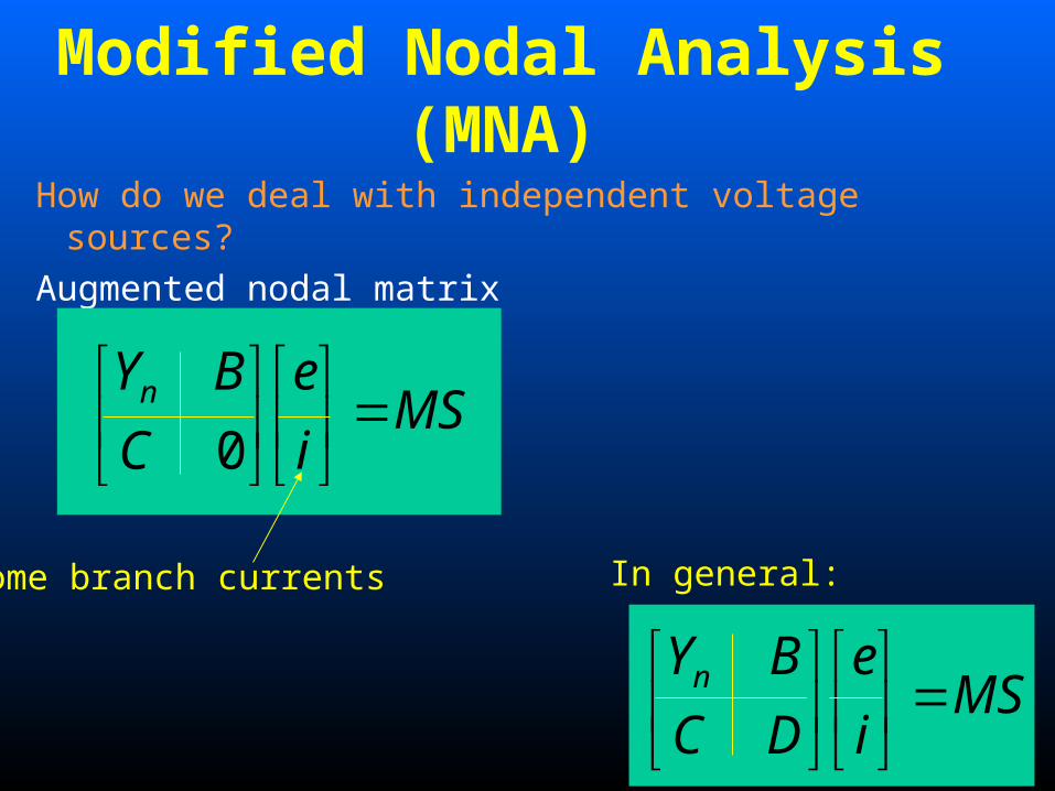
Modified Nodal Analysis (MNA)
How do we deal with independent voltage sources?
Augmented nodal matrix
MSi
e
C
BYn
0
Some branch currents
MSi
e
DC
BYn
In general:

MNA – General rules
• A branch current is always introduced as and additional variable for a voltage source or an inductor
• For current sources, resistors, conductors and capacitors, the branch current is introduced only if:– Any circuit element depends on that branch current– That branch current is requested as output
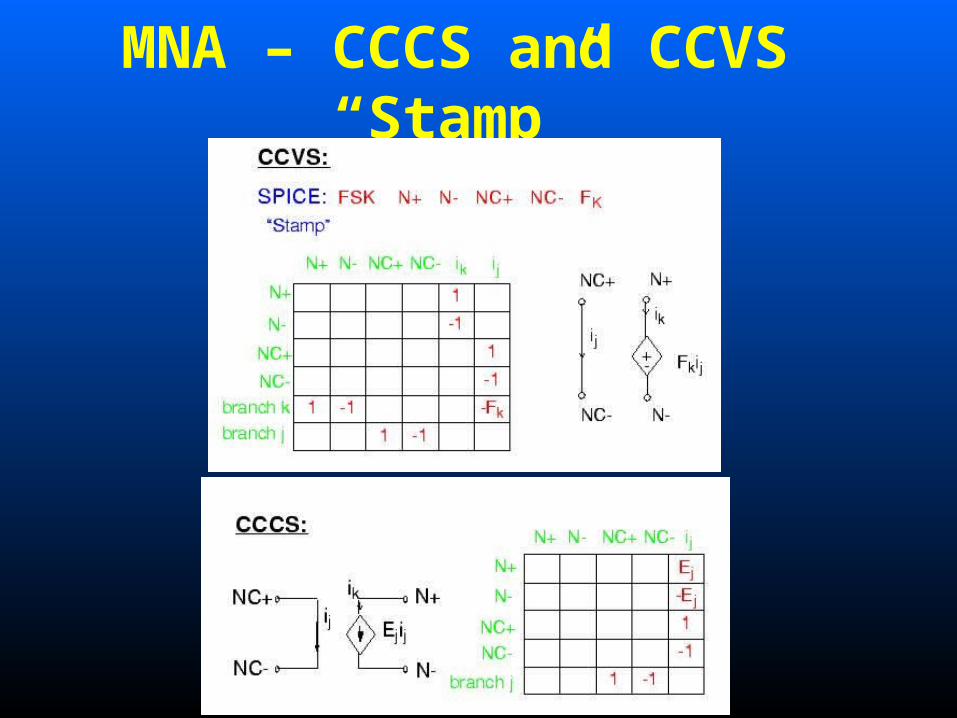
MNA – CCCS and CCVS “Stamp”

MNA – An example
0
1 2
G2v3
R4Is5R1
ES6- +
R8
3
E7v3
- +4
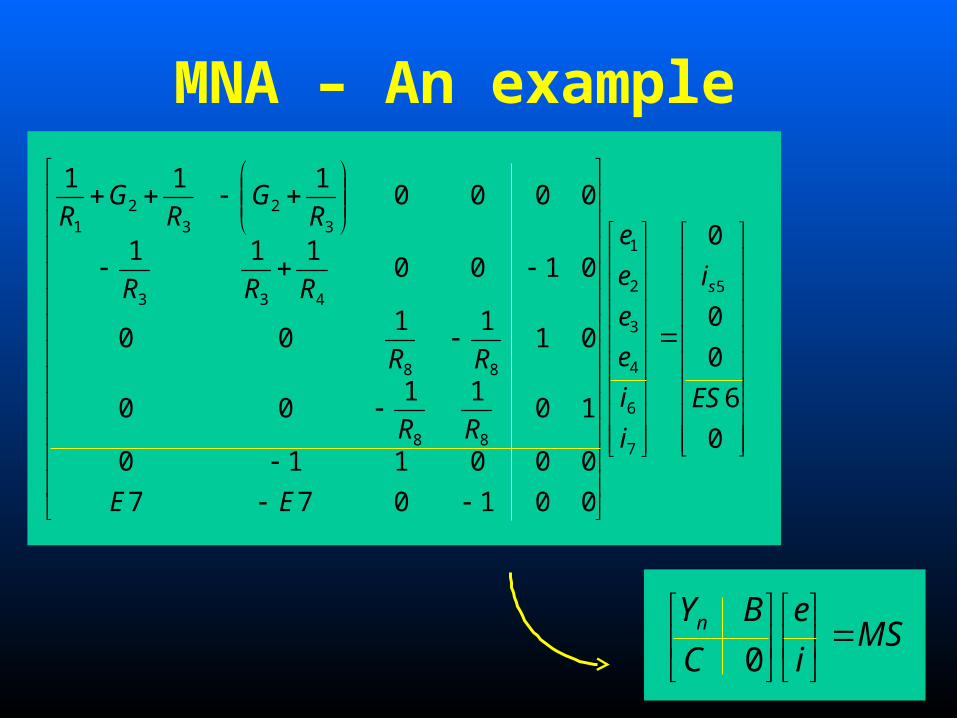
MNA – An example
0
6
0
0
0
001077
000110
1011
00
0111
00
0100111
0000111
5
7
6
4
3
2
1
88
88
433
32
32
1
ES
i
i
i
e
e
e
e
EE
RR
RR
RRR
RG
RG
R
s
MSi
e
C
BYn
0

Modified Nodal Analysis (MNA)
Advantages• MNA can be applied to any circuit• Eqns can be assembled directly from input
data• MNA matrix is close to Yn
Limitations• Sometimes we have zeros on the main
diagonal and principle minors may also be singular.
Systems of linear equations
• Problem to solve: M x = b
• Given M x = b :– Is there a solution?– Is the solution unique?

Systems of linear equations
Find a set of weights x so that the weighted sum of the
columns of the matrix M is equal to the right hand side b
1 1
2 21 2 N
N N
x b
x bM M M
x b
1 1 2 2 N Nx M x M x M b

Systems of linear equations - Existence
A solution exists when b is in the span of the columns of M
A solution exists if:
There exist weights, x1, …., xN, such that:
bMxMxMx NN ...2211
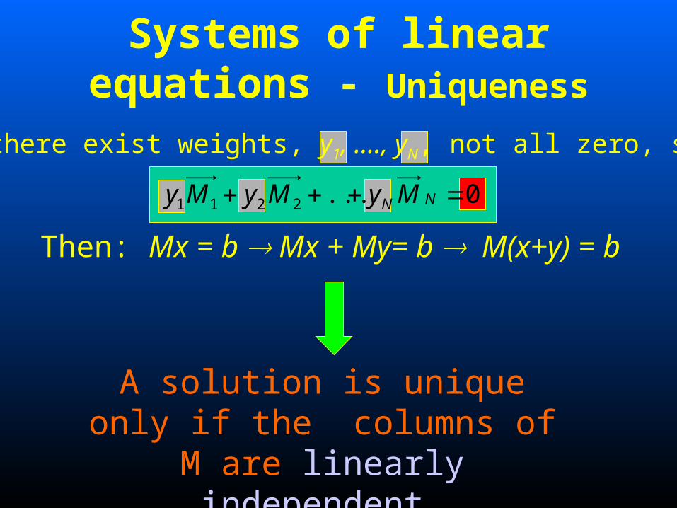
Systems of linear equations - Uniqueness
A solution is unique only if the columns of M are linearly
independent.
Then: Mx = b Mx + My= b M(x+y) = b
Suppose there exist weights, y1, …., yN, not all zero, such that:
0...2211 NN MyMyMy
Systems of linear equations Square matrices
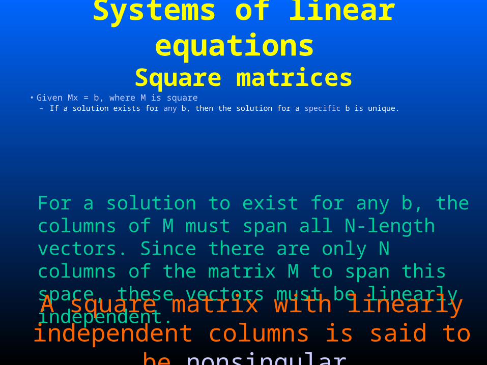
• Given Mx = b, where M is square– If a solution exists for any b, then the solution for a specific b is unique.
For a solution to exist for any b, the columns of M must span all N-length vectors. Since there are only N columns of the matrix M to span this space, these vectors must be linearly independent.
A square matrix with linearly independent columns is said to be nonsingular.

Application Problems
• Matrix is n x n• Often symmetric and diagonally dominant• Nonsingular of real numbers
bxM
SeY

Methods for solving linear equations
• Direct methods: find the exact solution in a finite number of steps
• Iterative methods: produce a sequence a sequence of approximate solutions hopefully converging to the exact solution

Gaussian Elimination Basics
Gaussian Elimination Method for Solving M x = b
• A “Direct” Method Finite Termination for exact result (ignoring roundoff)
• Produces accurate results for a broad range of matrices
• Computationally Expensive

GE basics: summary
(1) M x = b
U x = y Equivalent systemU: upper trg
(2) Noticed that:Ly = b L: unit lower trg
(3) U x = yLU x = b M x = b
GE
Efficient way of implementing GE: LU factorization

Solve M x = bStep 1
Step 2 Forward Elimination
Solve L y = bStep 3 Backward Substitution Solve U x = y
=M = L U
Gaussian Elimination Basics
Note: Changing RHS does not imply to recompute LU factorization
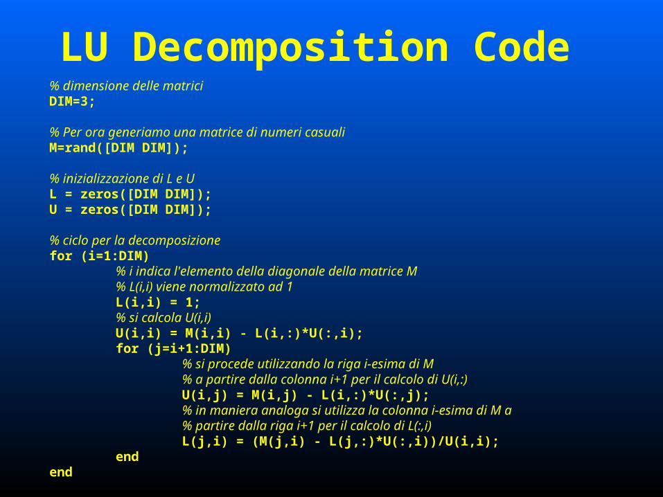
LU Decomposition Code% dimensione delle matriciDIM=3;
% Per ora generiamo una matrice di numeri casualiM=rand([DIM DIM]);
% inizializzazione di L e UL = zeros([DIM DIM]);U = zeros([DIM DIM]);
% ciclo per la decomposizionefor (i=1:DIM) % i indica l'elemento della diagonale della matrice M
% L(i,i) viene normalizzato ad 1 L(i,i) = 1; % si calcola U(i,i) U(i,i) = M(i,i) - L(i,:)*U(:,i); for (j=i+1:DIM) % si procede utilizzando la riga i-esima di M % a partire dalla colonna i+1 per il calcolo di U(i,:) U(i,j) = M(i,j) - L(i,:)*U(:,j); % in maniera analoga si utilizza la colonna i-esima di M a % partire dalla riga i+1 per il calcolo di L(:,i) L(j,i) = (M(j,i) - L(j,:)*U(:,i))/U(i,i); endend
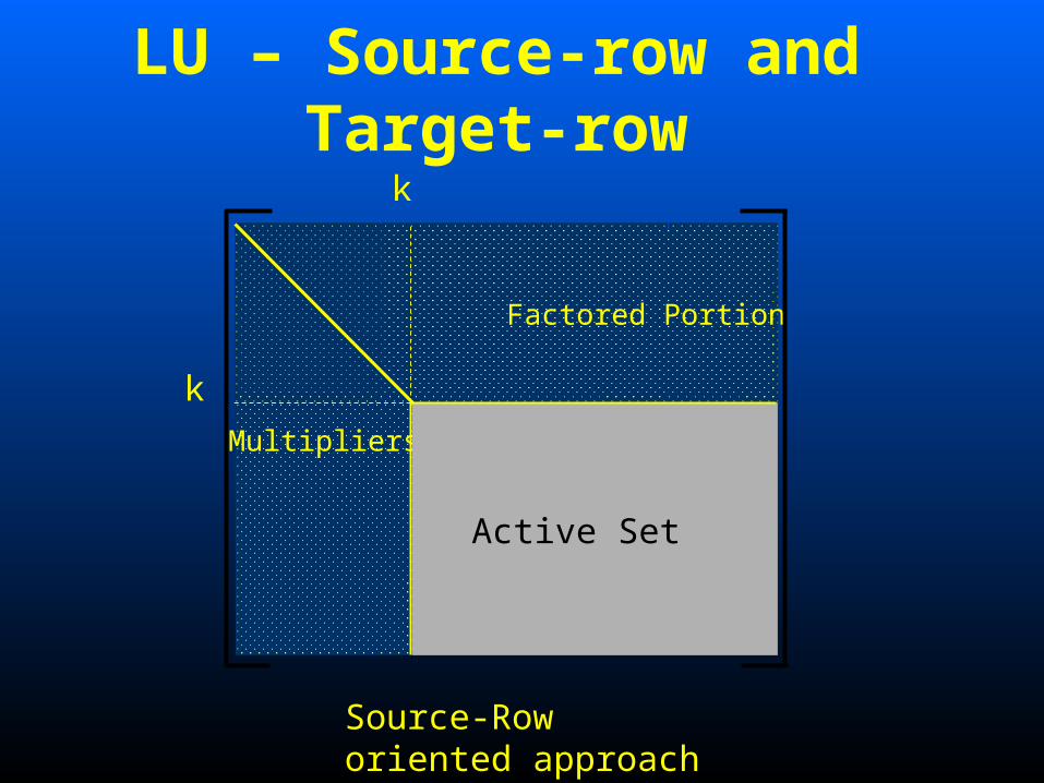
LU – Source-row and Target-row
Multipliers
Factored Portion
Active Set
k
k
Source-Row oriented approach
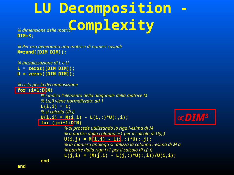
LU Decomposition - Complexity% dimensione delle matriciDIM=3;
% Per ora generiamo una matrice di numeri casualiM=rand([DIM DIM]);
% inizializzazione di L e UL = zeros([DIM DIM]);U = zeros([DIM DIM]);
% ciclo per la decomposizionefor (i=1:DIM) % i indica l'elemento della diagonale della matrice M
% L(i,i) viene normalizzato ad 1 L(i,i) = 1; % si calcola U(i,i) U(i,i) = M(i,i) - L(i,:)*U(:,i); for (j=i+1:DIM) % si procede utilizzando la riga i-esima di M % a partire dalla colonna i+1 per il calcolo di U(i,:) U(i,j) = M(i,j) - L(i,:)*U(:,j); % in maniera analoga si utilizza la colonna i-esima di M a % partire dalla riga i+1 per il calcolo di L(:,i) L(j,i) = (M(j,i) - L(j,:)*U(:,i))/U(i,i); endend
DIM3

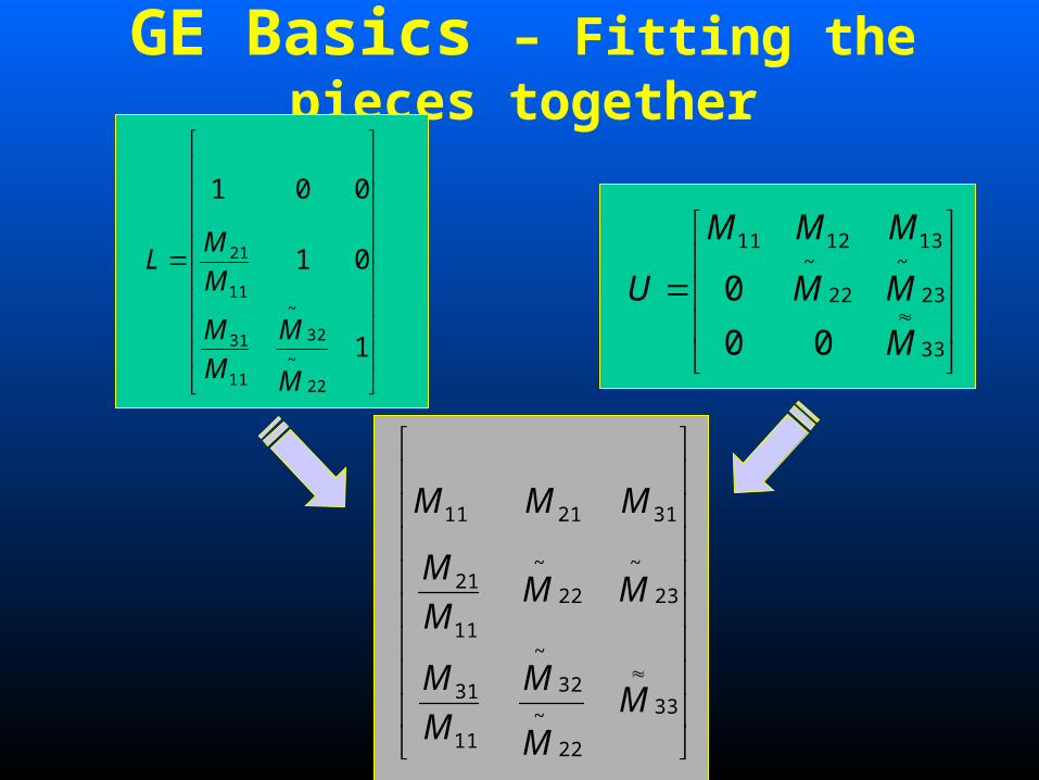
GE Basics – Fitting the pieces together
333231
232221
131211
MMM
MMM
MMM
33
23
~
22
~131211
00
0
M
MM
MMM
U
1
01
001
22
~
32
~
11
31
11
21
M
M
M
M
M
ML
GE Basics – Fitting the pieces together
33
23
~
22
~131211
00
0
M
MM
MMM
U
1
01
001
22
~
32
~
11
31
11
21
M
M
M
M
M
ML
33
22
~
32
~
11
31
23
~
22
~
11
21
312111
MM
M
M
M
MMM
M
MMM

LU Basics – Limitations of the naïve approach
• Zero Pivots
• Small Pivots (Round-off error)
both can be solved with partial pivoting

At Step i
Multipliers
Factored Portion
(L)iiM
jiM
Row i
Row j
What if Cannot form 0 ?iiM ji
ii
M
MSimple Fix (Partial Pivoting) If Find
0iiM 0jiM j i
Swap Row j with i
LU Basics – Partial pivoting for zero pivots
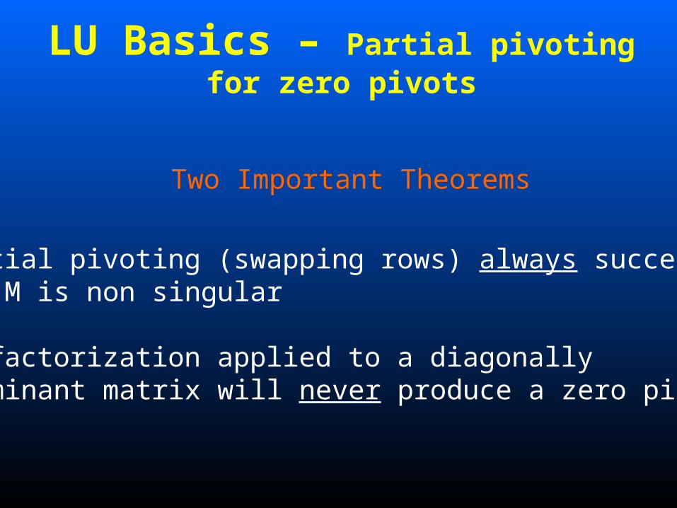
Two Important Theorems
1) Partial pivoting (swapping rows) always succeeds if M is non singular
2) LU factorization applied to a diagonally dominant matrix will never produce a zero pivot
LU Basics – Partial pivoting for zero pivots
Summary
• Existence and uniqueness review
• Gaussian elimination basics– GE basics– LU factorization– Pivoting


![[Malik et al 1988] Malik, S., Wang, A., Brayton, R. K ... › ~bryant › pubdir › CMU-CS-92-160.pdf[Malik et al 1988] Malik, S., Wang, A., Brayton, R. K., and Sangiovanni-Vincentelli,](https://static.documents.pub/doc/80x56/5f0cd6787e708231d437611b/malik-et-al-1988-malik-s-wang-a-brayton-r-k-a-bryant-a-pubdir.jpg)

