Thesis submitted to the Graduate Division of the Electrical Engeneering Faculty of the Federal University of Uberlândia as a fulfillment of the requirements for the PhD degree in the area of Artificial Intelligence of the course of Graduation in Electrical Engineering. José Romildo Malaquias Computer Algebra in Modern Functional Languages Prof. Dr. Antônio Eduardo Costa Pereira Thesis Supervisor Universidade Federal de Uberlândia Uberlândia, MG Brazil February 26 2007
Transcript
Thesis submitted to the Graduate Division of the Electrical Engeneering Faculty of the Federal
University of Uberlândia as a fulfillment of the requirements for the PhD degree in the area of
Artificial Intelligence of the course of Graduation in Electrical Engineering.
José Romildo Malaquias
Computer Algebra in Modern Functional
Languages
Prof. Dr. Antônio Eduardo Costa Pereira
Thesis Supervisor
Universidade Federal de Uberlândia
Uberlândia, MG
Brazil
February 26 2007
Dados Internacionais de Catalogação na Publicação (CIP)
M237c Malaquias, José Romildo, 1967- Computer algebra in modern functional languages / José Romildo Malaquias. - 2007. 140 f. : il.
Orientador: Antonio Eduardo Costa Pereira.
Tese (doutorado) – Universidade Federal de Uberlândia, Programa de Pós-Graduação em Engenharia Elétrica. Inclui bibliografia.
1. Inteligência artificial - Teses. 2. Programação funcional (Computa-ção) - Teses. I. Pereira, Antonio Eduardo Costa. II. Universidade Federal de Uberlândia. Programa de Pós-Graduação em Engenharia Elétrica. III. Título. CDU: 681.3:007.52
Elaborado pelo Sistema de Bibliotecas da UFU / Setor de Catalogação e Classificação
Computer Algebra in Modern Functional
Languages
José Romildo Malaquias
Composition of the Examining Board
Prof. Dr. Antônio Eduardo Costa Pereira FEELT – UFU Supervisor
struggle to become the standard dialect of the main AI language. In the mean time,
Macsyma migrated from MACLISP to Common Lisp. The result is that Macsyma runs in
a standard language, while Reduce is built on top of an obscure dialect known as Standard
Lisp.
• Maple3. Lisp always had a bad reputation for being slow. Therefore, Maple [11] was
developed (at the University of Waterloo, Canada) in a procedural language (C) with a
view to greater efficiency. Since procedural languages like C are not fit for symbolic
computation, the implementors of Maple were forced to invent a symbolic language. Not
being experts in compiler construction, they wrote an interpreter for the Maple language.
The result is that Maple is much slower than Macsyma and other Lisp based systems.
Maple’s source code is not in the public domain.
• Derive4. This package (and its precursor MuMATH) was designed to offer a small and
fast Computer Algebra system [12]. It was the only competitor to Macsyma that really
delivered its promises. The system is indeed very small and reasonably fast. However, it
did not meet the commercial success of Reduce and Maple.
Maple, Reduce and Derive were designed to be worthy competitors of Macsyma. There are
also systems designed to offer limited functionality in a friendly environment. Among these
systems, MatLab5 [13] and Mathematica6 [14] became imensily popular.
It is interesting to note that these two systems that promised limited functionality failed to
deliver their promise too. Due to demands from the market, the developers of both MatLab
and Mathematica increased the functionality of their systems, which became as fat as Reduce.
However, neither MatLab nor Mathematica have the well designed architecture of Reduce. In
fact, these system suffered from a chaotic growth.
Other systems are:
• Magma7. Magma is a large software package designed to solve computationally hard3http://www.maplesoft.com/4http://www.derive.com/5http://www.mathworks.com/6http://www.mathematica.com/7http://www.maths.usyd.edu.au/u/magma/
Chapter three: Addition Explains the fundamental algorithms of the system for addition.
Chapter four: Multiplication and Subtraction. Discusses the algorithms used in symbolic
multiplication and the use of the multiplication by -1 to achieve the subtraction.
Chapter five: Exponentiation and Division Presents the algorithms used both in exponentia-
tion and in division.
Chapter six: System Organization Presents the module structure of the system and the re-
sults of a benchmarking program.
Chapter seven: Conclusion and Future Work Presents the conclusion and suggestions for
future works.
Chapter 2Algebraic Formulas
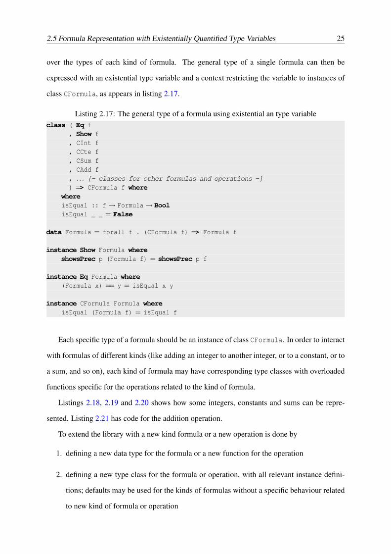
In this chapter, the reader will find descriptions abstract representations of the algebraic expres-
sions in our Computer Algebra library. The author will be specially concerned with the basic
manipulations of the foresaid expressions, but he will also discuss the result of computations
that may fail or succeed.
For the sake of clarity, the term formula will be used for algebraic expression, as expres-
sion is already used when discussing programming languages and denotes a construct of the
language not necessarily related to Algebra. This avoids ambiguity in terminology.
2.1 Kinds of Formulas
Formulas are expressions that can be manipulated in Algebra. They can be added and multi-
plied. They can be squared. Trignometric transformations may be applied to them. They can be
diferentiated and integrated. A large number of operations can be applied to formulas. Formulas
may be composed by numbers and variables, which can be combined in different ways.
Formulas can be grouped, according to their structure, in several groups, including:
• Integers, corresponding to the integer numbers, as defined in axiomatic theories like
Peano’s axioms, Church’s numbers, or in one of the many brands of the Set Theory. A
few examples of this group are 416, 7453 and −3291.
• Constants, representing known mathematical entities. They are expressed by a symbol or
12
2.1 Kinds of Formulas 13
a name, like π, e (neperian number) and ı (imaginary unit). In general, a constant formula
stands for a number without an exact representation in a given numeric system.
• Variables, corresponding closely to mathematical variables. Logicians call them literals
more often than not. Examples of literals: x, y, a, b, α, β.
• Applications, which are formulas built from simpler formulas by applying a functional
operator to its arguments, which are themselves formulas. Exemplos: sinx, cothx, lnx,
log10 x, x + 2, −a, π2 and 5× sin[3π(α + 2)]. Applications may have different forms,
depending on the operator. The basic arithmetic applications are
– Sum, denoting the sum of two formulas. Examples are a+b and 13+ y×4x.
– Product, denoting the product of two formulas. For example 4× x and (a + b)×
(a+ c).
– Power, denoting the power of two formulas, as in x2 and (a+b)12 .
There is no need for special forms for differences and quotients: they can be expressed
using the above formulas. Basicaly, for any formulas x and y,
x− y = x+(−1)× y
xy
= x× y−1
Other common applications are
– Logarithm of a formula in a given base. Examples are log10 y, loge(x + y) and
logb bc.
– Trigonometric formulas, like sine, cosine and tangent of a formula. Examples:
sinx, cosa2, tan(x2 + y2).
There are many other possible forms of applications (hyperbolic formulas, derivatives,
integrals, vectors, matrices, series, . . . )
14 2 Algebraic Formulas
• Indeterminates, which are formulas whose value cannot be determined, like those ob-
tained by dividing by zero. Examples are 3/0, 00 and log0x.
2.2 Trivial Representation of Formulas
The representation of formulas in the implementation language is tricky. One could simply use
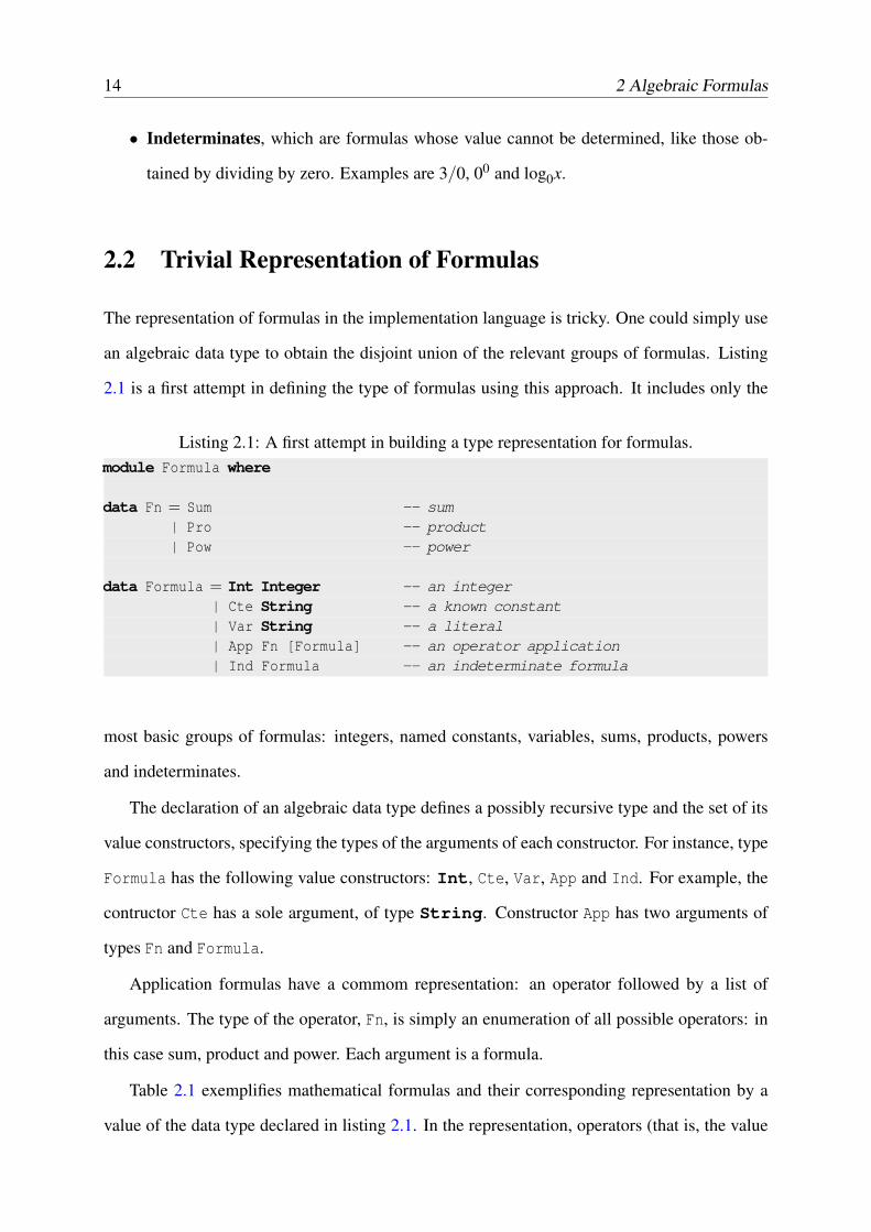
an algebraic data type to obtain the disjoint union of the relevant groups of formulas. Listing
2.1 is a first attempt in defining the type of formulas using this approach. It includes only the
Listing 2.1: A first attempt in building a type representation for formulas.module Formula where
data Fn = Sum -- sum| Pro -- product| Pow -- power
data Formula = Int Integer -- an integer| Cte String -- a known constant| Var String -- a literal| App Fn [Formula] -- an operator application| Ind Formula -- an indeterminate formula
most basic groups of formulas: integers, named constants, variables, sums, products, powers
and indeterminates.
The declaration of an algebraic data type defines a possibly recursive type and the set of its
value constructors, specifying the types of the arguments of each constructor. For instance, type
Formula has the following value constructors: Int, Cte, Var, App and Ind. For example, the
contructor Cte has a sole argument, of type String. Constructor App has two arguments of
types Fn and Formula.
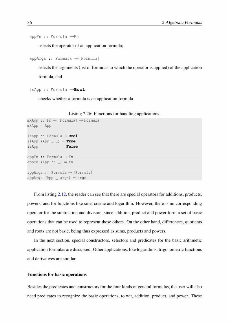
Application formulas have a commom representation: an operator followed by a list of
arguments. The type of the operator, Fn, is simply an enumeration of all possible operators: in
this case sum, product and power. Each argument is a formula.
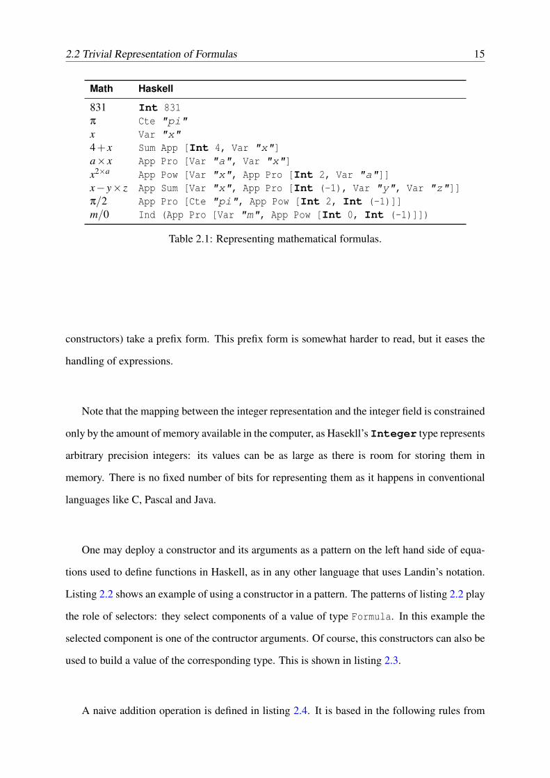
Table 2.1 exemplifies mathematical formulas and their corresponding representation by a
value of the data type declared in listing 2.1. In the representation, operators (that is, the value
2.2 Trivial Representation of Formulas 15
Math Haskell
831 Int 831π Cte "pi"x Var "x"4+ x Sum App [Int 4, Var "x"]a× x App Pro [Var "a", Var "x"]x2×a App Pow [Var "x", App Pro [Int 2, Var "a"]]x− y× z App Sum [Var "x", App Pro [Int (-1), Var "y", Var "z"]]π/2 App Pro [Cte "pi", App Pow [Int 2, Int (-1)]]m/0 Ind (App Pro [Var "m", App Pow [Int 0, Int (-1)]])
Table 2.1: Representing mathematical formulas.
constructors) take a prefix form. This prefix form is somewhat harder to read, but it eases the
handling of expressions.
Note that the mapping between the integer representation and the integer field is constrained
only by the amount of memory available in the computer, as Hasekll’s Integer type represents
arbitrary precision integers: its values can be as large as there is room for storing them in
memory. There is no fixed number of bits for representing them as it happens in conventional
languages like C, Pascal and Java.
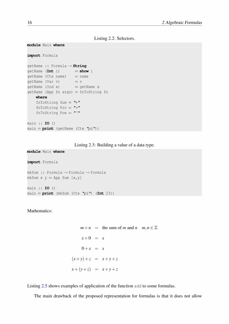
One may deploy a constructor and its arguments as a pattern on the left hand side of equa-
tions used to define functions in Haskell, as in any other language that uses Landin’s notation.
Listing 2.2 shows an example of using a constructor in a pattern. The patterns of listing 2.2 play
the role of selectors: they select components of a value of type Formula. In this example the
selected component is one of the contructor arguments. Of course, this constructors can also be
used to build a value of the corresponding type. This is shown in listing 2.3.
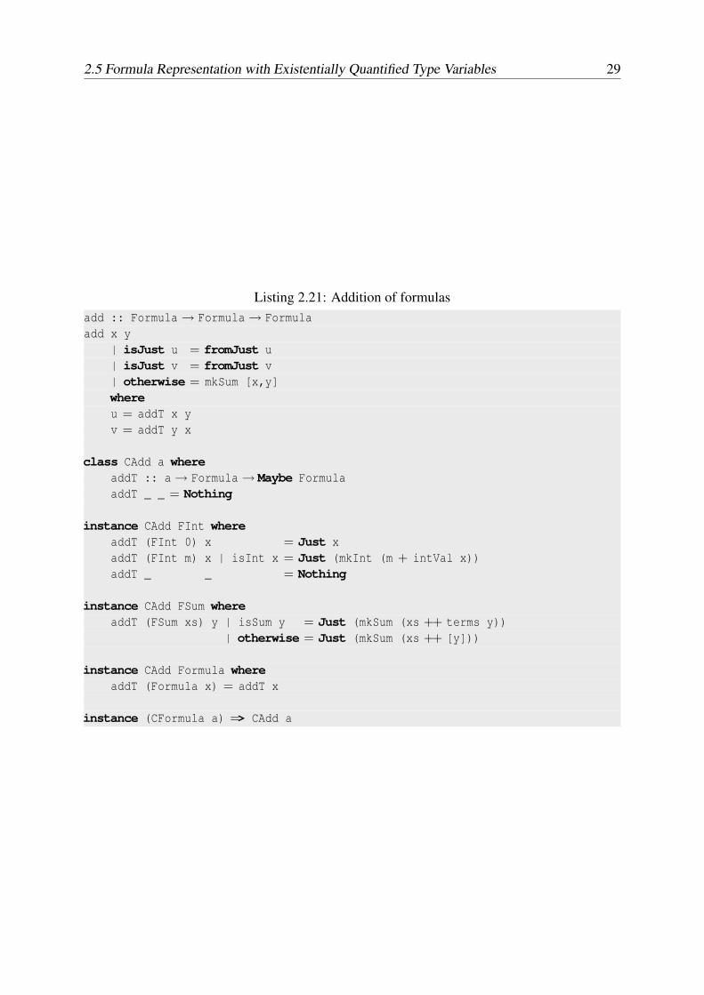
A naive addition operation is defined in listing 2.4. It is based in the following rules from
Listing 2.5 shows examples of application of the function add to some formulas.
The main drawback of the proposed representation for formulas is that it does not allow
2.2 Trivial Representation of Formulas 17
Listing 2.4: Addition of two formulasadd :: Formula→ Formula→ Formulaadd (Int m) (Int n) = Int (m + n)add x (Int 0) = xadd (Int 0) x = xadd (App Sum xs) (App Sum ys) = App Sum (xs ++ ys)add x (App Sum ys) = App Sum (x:ys)add (App Sum xs) y = App Sum (y:xs)add x y = App Sum [x,y]
Listing 2.5: Examples of addition of formulasx1, x2, x3, x4, x5, x6 :: Formulax1 = add (Int 81) (Int 12) -- Int 93x2 = add (Cte "pi") (Int 0) -- Cte "pi"x3 = add (Int 0) (Var "alfa") -- Var "alfa"x4 = add (App Sum [Int 5, Var "x"])
(App Sum [Cte "e", Var "y"]) -- App Sum [Int 5, Var "x", Cte "e", Var "y"]x5 = add (Var "x")
(App Sum [Int 7, Var "y"]) -- App Sum [Var "x", Int 7, Var "y"]x6 = add (App Sum [Int 5, Var "x"])
(Cte "pi") -- App Sum [Int 5, Var "x", Cte "pi"]
easy extension of the type Formula without affecting all programs alreading using this type.
Certainly the library will not offer all possible groups of formulas and someone probably would
like to extended it. For example, suppose the library does not deal with logarithms and the user
wishes to add support for them (effectively extending the library). A new value constructor for
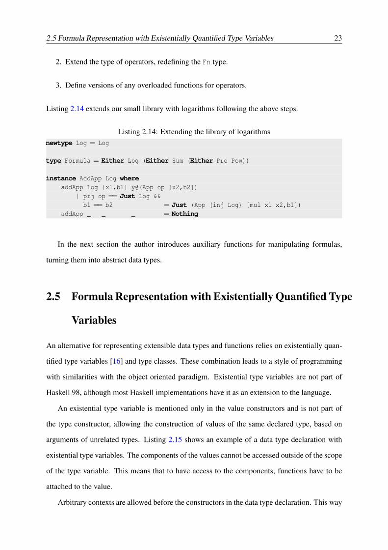
logarithms should be added in the definition of type Fn. Also new rules may need to be added
in the relevant function definitions. Listing 2.6 shows an updated definition for the type of
operators. Listing 2.7 shows an extended addition operation capable of adding two logarithms
Listing 2.6: Adding logarithms to the formula representation.data Fn = Sum -- sum
| Pro -- product| Pow -- power| Log -- logarithms
in the same base, according to the following mathematical law.
logb x+ logb y = logb(x× y)
18 2 Algebraic Formulas
Listing 2.7: Addition od formulas, including derivatives.add :: Formula→ Formula→ Formulaadd (Int m) (Int n) = Int (m + n)add x (Int 0) = xadd (Int 0) x = xadd (App Log x b1) (App Log y b2) = if b1 == b2
then App Log [mul x y, y1]else App Sum [App Log [x,b1], App Log [y,b2]]
add (App Sum xs) (App Sum ys) = App Sum (xs ++ ys)add x (App Sum ys) = App Sum (x:ys)add (App Sum xs) y = App Sum (y:xs)add x y = App Sum [x,y]
mul :: Formula→ Formula→ Formulamul = . . .
Many kinds of formulas and the related operations may be implemented in the library:
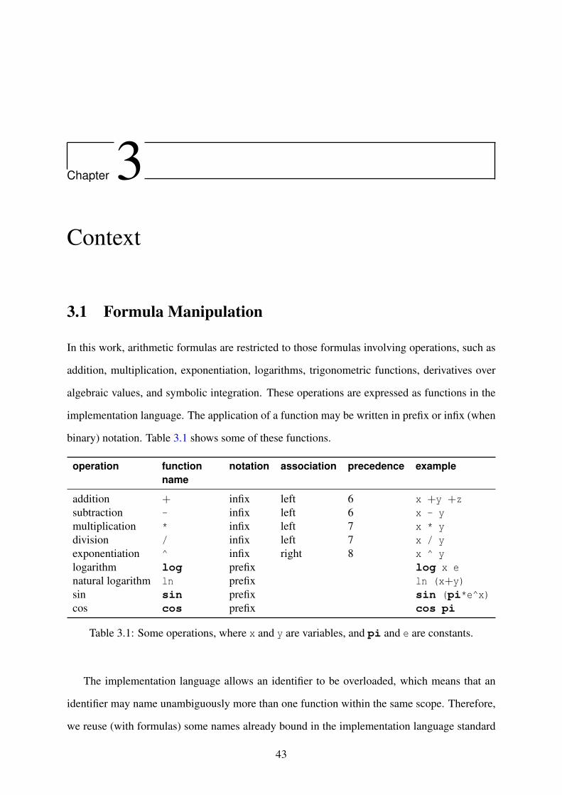
In this work, arithmetic formulas are restricted to those formulas involving operations, such as
addition, multiplication, exponentiation, logarithms, trigonometric functions, derivatives over
algebraic values, and symbolic integration. These operations are expressed as functions in the
implementation language. The application of a function may be written in prefix or infix (when
binary) notation. Table 3.1 shows some of these functions.
operation functionname
notation association precedence example
addition + infix left 6 x +y +zsubtraction - infix left 6 x - ymultiplication * infix left 7 x * ydivision / infix left 7 x / yexponentiation ^ infix right 8 x ^ ylogarithm log prefix log x enatural logarithm ln prefix ln (x+y)sin sin prefix sin (pi*e^x)cos cos prefix cos pi
Table 3.1: Some operations, where x and y are variables, and pi and e are constants.
The implementation language allows an identifier to be overloaded, which means that an
identifier may name unambiguously more than one function within the same scope. Therefore,
we reuse (with formulas) some names already bound in the implementation language standard
43
44 3 Context
environment, like + and sin, for the addition operation and the sine function respectively.
In Haskell, these two functions are defined for the builtin numeric types, i.e., for Int and
Float. When the overloaded names have an infix notation, the association and precedence
are defined in the implementation language standard environment. By doing so, we make sure
that the notation used to express operations over formulas resembles the mathematical notation
as far as possible, and the mathematical notation should be preferred in computational algebra
systems. In this thesis the implementation language notation is used only when it illuminates
the discussion, or simplifies handling of formulas by the machine. When feasible, the author
prefers the pure mathematical notation over the implementation language notation.
A few examples of evaluation of formulas applying arithmetic operations follow.
2+35
+8x3
x− x2 ⇒ 13
5+7x2 (3.1)
a(a+b)⇒ a2 +ab (3.2)
lnx5− lnx⇒ 4lnx (3.3)
sin2(x+ y)+ cos2(x+ y)⇒ 1 (3.4)
The examples show that a computer algebra system is supposed to symplify any formula
that cannot be reduced to a number. In general, a formula can be simplified in different ways,
producing different results. For example, the formula
b2 · ab
+aa+bb+ab
can be simplified to result in
a2 +2ab+b2
or in
(a+b)2
This issue is investigated in the next section. For the time being, we will take a look at listing
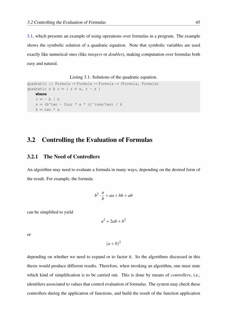
3.2 Controlling the Evaluation of Formulas 45
3.1, which presents an example of using operations over formulas in a program. The example
shows the symbolic solution of a quadratic equation. Note that symbolic variables are used
exactly like numerical ones (like integers or doubles), making computation over formulas both
easy and natural.
Listing 3.1: Solutions of the quadratic equation.quadratic :: Formula→ Formula→ Formula→ (Formula, Formula)quadratic a b c = ( r + s, r - s )
wherer = - b / ks = (b^two - four * a * c)^(one/two) / kk = two * a
3.2 Controlling the Evaluation of Formulas
3.2.1 The Need of Controllers
An algorithm may need to evaluate a formula in many ways, depending on the desired form of
the result. For example, the formula
b2 · ab
+aa+bb+ab
can be simplified to yield
a2 +2ab+b2
or
(a+b)2
depending on whether we need to expand or to factor it. So the algorithms discussed in this
thesis would produce different results. Therefore, when invoking an algorithm, one must state
which kind of simplification is to be carried out. This is done by means of controllers, i.e.,
identifiers associated to values that control evaluation of formulas. The system may check these
controllers during the application of functions, and build the result of the function application
46 3 Context
according to the values of the controllers. The set of all controllers forms the context in which
formulas are calculated.
3.2.2 Representing Contexts
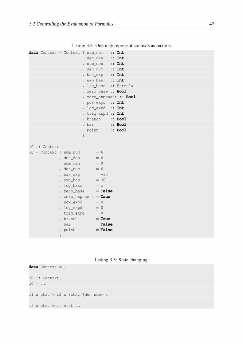
The contexts are states represented as records in the implementation language. Each controller
is a field in the record. The value of a controller is the value of the corresponding field. Listing
3.2 shows an example of context. This initial context is bound to a global variable, since it may
be used whenever one needs to restart a chain of state changes.
From listing 3.2, the reader can see that the notation to access a given controller is function
application, to wit:
controller context
At the beginning of this section, it was said that context is a state representation. This means
that the programmer may change one or more fields of the initial context. If we were dealing
with a procedural language, or even with a functional language with mutable data structures, we
would change the global context directly. Haskell, as well as other purely functional languages,
does not allow this, in order to guarantee referential transparency. However, one may pass the
context as argument to a function and change it in the context of a new call. Listing 3.3 gives
an example of a function which changes the context. From that listing, the reader can see that
the syntax for changing a set of selcted fields, while maintaining the others, has the following
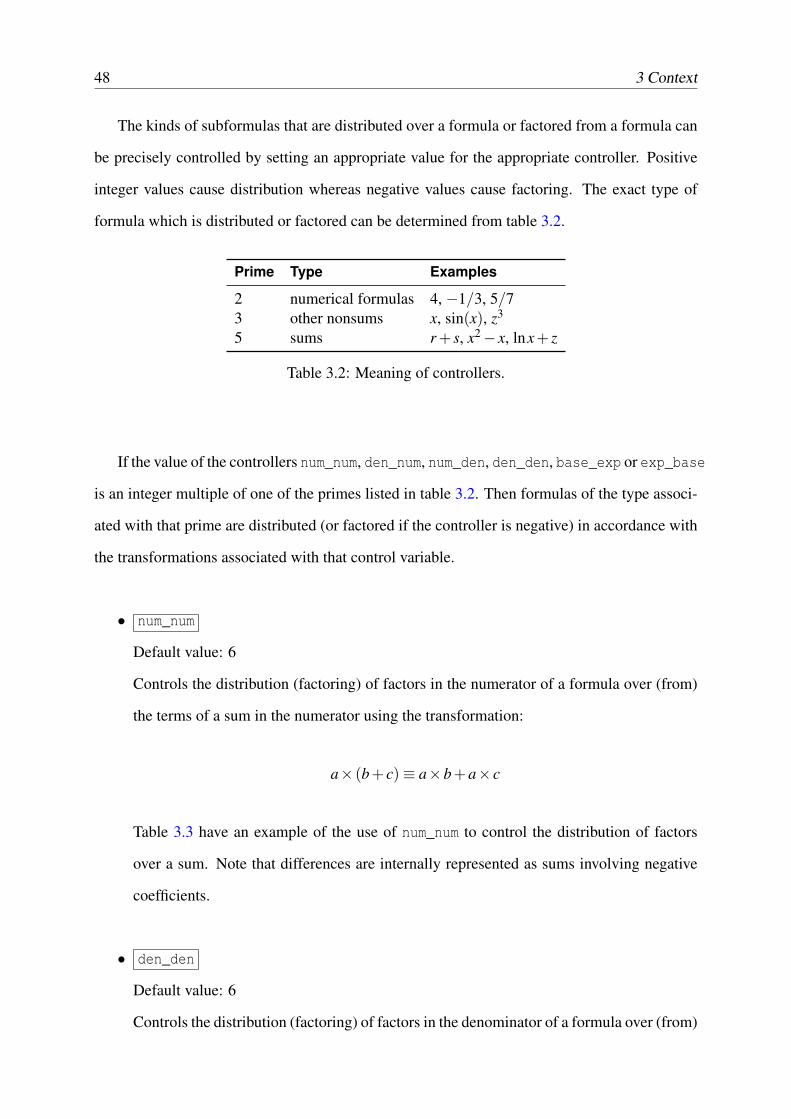
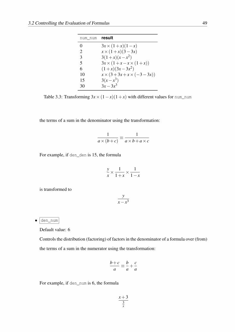
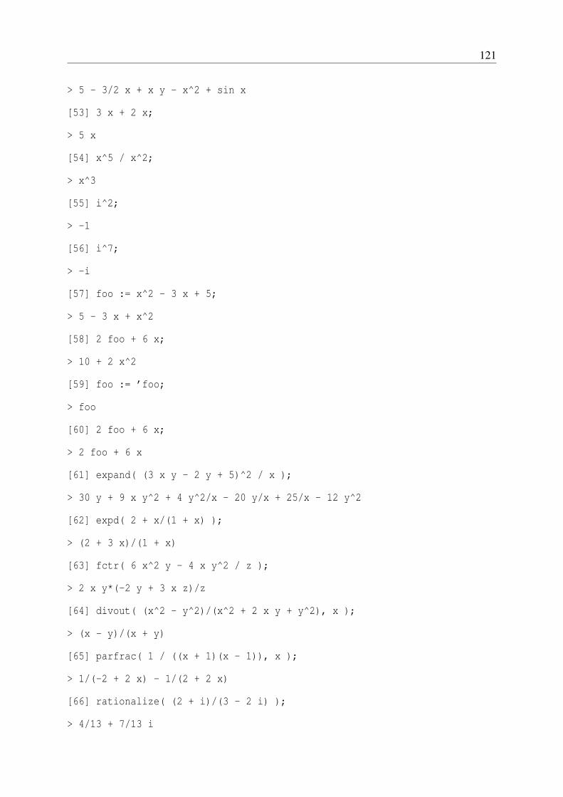
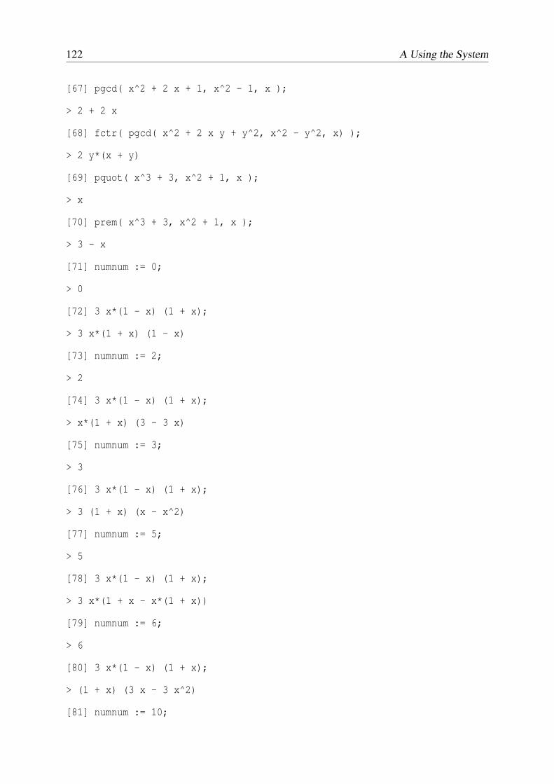
Table 3.3: Transforming 3x× (1− x)(1+ x) with different values for num_num
the terms of a sum in the denominator using the transformation:
1a× (b+ c)
≡ 1a×b+a× c
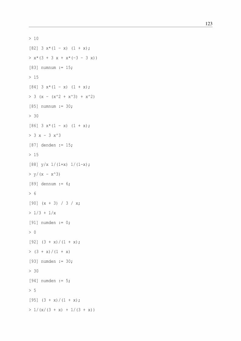
For example, if den_den is 15, the formula
yx× 1
1+ x× 1
1− x
is transformed toy
x− x3
• den_num
Default value: 6
Controls the distribution (factoring) of factors in the denominator of a formula over (from)
the terms of a sum in the numerator using the transformation:
b+ ca
≡ ba
+ca
For example, if den_num is 6, the formula
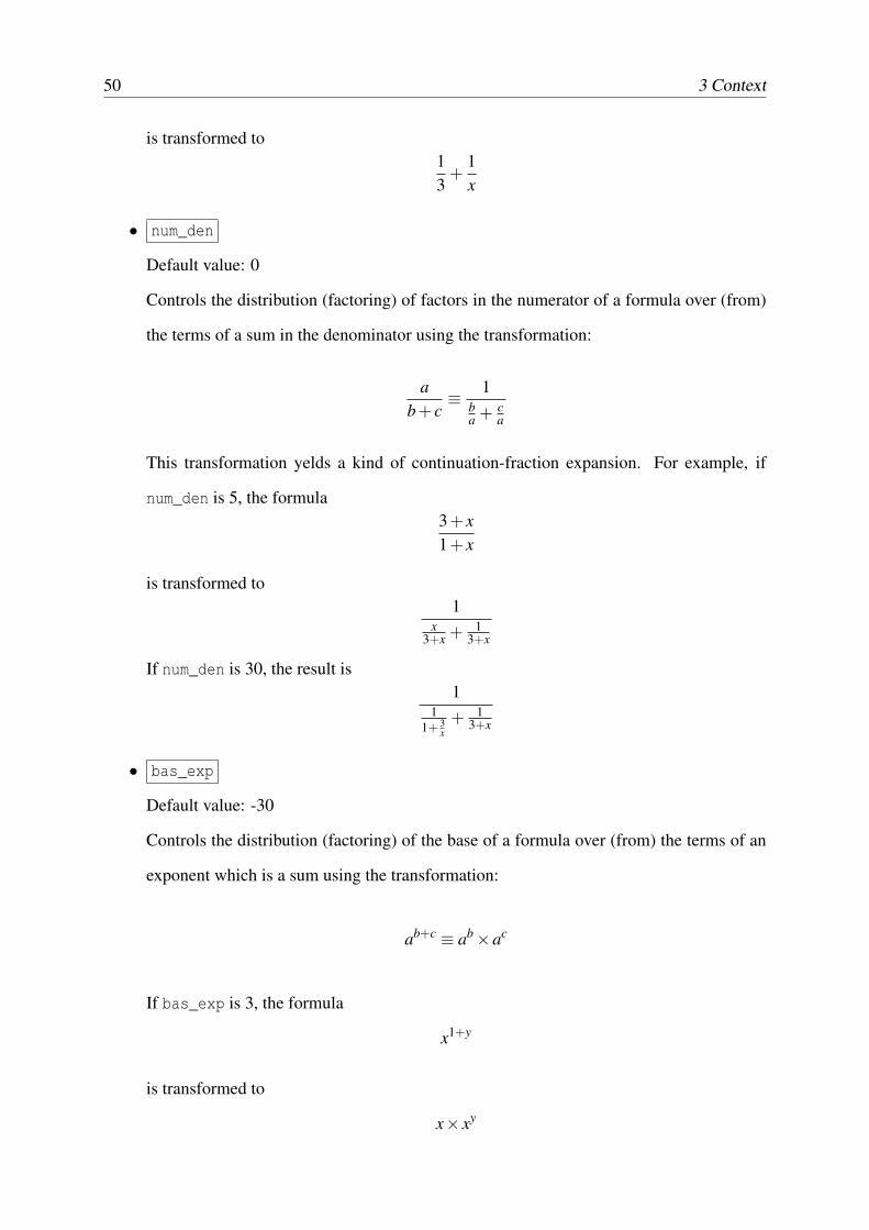
x+33x
50 3 Context
is transformed to13
+1x
• num_den
Default value: 0
Controls the distribution (factoring) of factors in the numerator of a formula over (from)
the terms of a sum in the denominator using the transformation:
ab+ c
≡ 1ba + c
a
This transformation yelds a kind of continuation-fraction expansion. For example, if
num_den is 5, the formula3+ x1+ x
is transformed to1
x3+x + 1
3+x
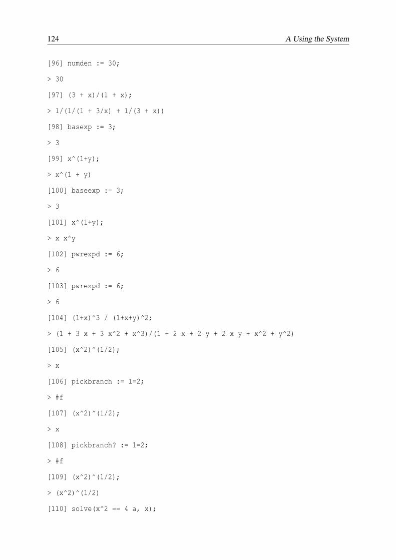
If num_den is 30, the result is1
11+ 3
x+ 1
3+x
• bas_exp
Default value: -30
Controls the distribution (factoring) of the base of a formula over (from) the terms of an
exponent which is a sum using the transformation:
ab+c ≡ ab×ac
If bas_exp is 3, the formula
x1+y
is transformed to
x× xy
3.2 Controlling the Evaluation of Formulas 51
If bas_exp is a negative integer, common bases are collected under an exponent. Since
this transformation is usually more desirable, the default value for bas_exp is -30.
• exp_bas
Default value: 0
Controls the distribution (factoring) of the exponent of a formula over (from) the base
using the transformation:
(a×b)c ≡ ac×bc
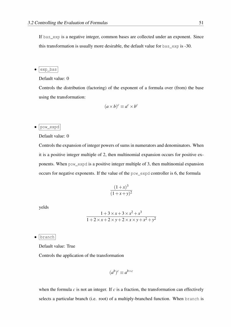
• pow_expd
Default value: 0
Controls the expansion of integer powers of sums in numerators and denominators. When
it is a positive integer multiple of 2, then multinomial expansion occurs for positive ex-
ponents. When pow_expd is a positive integer multiple of 3, then multinomial expansion
occurs for negative exponents. If the value of the pow_expd controller is 6, the formula
(1+ x)3
(1+ x+ y)2
yelds1+3× x+3× x2 + x3
1+2× x+2× y+2× x× y+ x2 + y2
• branch
Default value: True
Controls the application of the transformation
(ab)c ≡ ab×c
when the formula c is not an integer. If c is a fraction, the transformation can effectively
selects a particular branch (i.e. root) of a multiply-branched function. When branch is
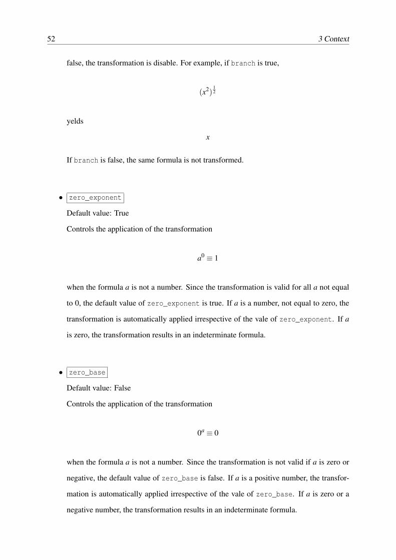
52 3 Context
false, the transformation is disable. For example, if branch is true,
(x2)12
yelds
x
If branch is false, the same formula is not transformed.
• zero_exponent
Default value: True
Controls the application of the transformation
a0 ≡ 1
when the formula a is not a number. Since the transformation is valid for all a not equal
to 0, the default value of zero_exponent is true. If a is a number, not equal to zero, the
transformation is automatically applied irrespective of the vale of zero_exponent. If a
is zero, the transformation results in an indeterminate formula.
• zero_base
Default value: False
Controls the application of the transformation
0a ≡ 0
when the formula a is not a number. Since the transformation is not valid if a is zero or
negative, the default value of zero_base is false. If a is a positive number, the transfor-
mation is automatically applied irrespective of the vale of zero_base. If a is zero or a
negative number, the transformation results in an indeterminate formula.
3.2 Controlling the Evaluation of Formulas 53
3.2.4 Referential Transparency
In section 3.2.2, we have said that Haskell does not allow changing in a global value. This
means that Haskell does not allow destructive updates of the value refered by a given vari-
able. Although possible in other languages, destructive updating should be avoided, because it
obscures the meaning of the program. To understand this, one must refer to books of Philos-
ophy, where one discusses the concept of referential transparency. Bertrand Russel says that a
language has referential transparency if one can substitute an expression’s subexpression with
another of equal meaning, preserving the meaning of the original expression. Since substitu-
tion is a fundamental operation in logic reasoning, a computer language must exhibit referential
transparency if we ever want to reason about programs. An example from Russel will make
clear what is referential transparency. Consider the following sentence:
George IV wanted to know whether Scott was the author of Waverley.
Historians say that this sentence is true, i. e., George IV really wanted to know whether Scott
had written Waverley. We know that Walter Scott was the author of Waverley. Therefore, the
name Scott and the noun phrase author of Waverley are equivalent expressions, i.e., they refer
to the same person. Therefore, if English is transparent, one can substitute Scott for author of
Waverley. With this substitution, Russel’s sentence becomes:
George IV wanted to know whether Scott was Scott.
After the substitution, the sentence, which was true, becomes false. Of course, George IV
did not want to know whether Scott was Scott. Even being mad, George IV knew perfectly well
that Scott was indeed Scott. The replacement of an expression for its equivalent may falsify
a true sentence! The conclusion we reach is that, if a language is not transparent, one cannot
substitute equals for equals. Although acceptable in a natural language, this is undesirable
in a programming language, because programmers must use substitutions to prove their code
correct, or to perform source to source transformation. To understand this, consider the small
program of listing 3.4. One cannot substitute g(2)+h(5) for h(5)+g(2), even though the
commutative property of the addition operation warranties this equivalence.
54 3 Context
Listing 3.4: Procedural languages are not transparent.program (input,output);var y = 5;
function g(integer x): integer;begin
y := 512;g := 2 * x
end;
function h(integer x): integer;begin
h := x + yend;
beginwriteln(h(5)+ g (2))
end.
3.2.5 Passing the Context as Input to Algorithms
It was said that the algorithms we are using make use of contexts to control simplification of
formulas. Basically the controller’s values are set with the desired values (the ones that will
produce the desired result form) and then the simplification of formulas takes place in this
customized context. The implementation of the algorithms may use the context in two ways:
• consult the value of some controller in the context and conduct simplification of the for-
mulas according to the controllers value,
• create a new context on which formulas are simplified and their results are used to build
the final result
Imperative programming languages are based on state changing. In such languages a vari-
able is a placeholder that contains a value. The value is stored in the variable using assignment
commands. Pascal, C, Java, Lisp, Scheme and ML are examples of imperative programming
languages. In section 3.2.4, we have learned that this kind of destructive update leads to an un-
desirable situation, where reasoning about programs becomes very difficult. On the other hand,
the use of contexts in procedural languages is trivial: the context may be stored as a value in
a global variable. This variable could be accessed directly from any function that requires the
3.2 Controlling the Evaluation of Formulas 55
value of a controller. To produce a new context, first the original context should be stored in
a temporary variable and then it can be changed as desired. Further simplification of formulas
will use this modified context. When it is not needed anymore, the original context saved in
the temporary variable is restored, and simplification can continue. This technique of saving
and restoring the context is accomplished automatically in languages with dynamic scope for
variables (like Lisp and some Scheme dialects).
Declarative languages do not support the concept of state changing and variables are just
names for unknown, but otherwise fixed values. The values they represent cannot be changed.
Logic and (pure) functional languages like Mercury, and Haskell are declarative. A solution to
our problem would be to pass the context as an extra argument to the functions which manipulate
formulas, as hinted in listing 3.3. If a new context is needed, it can be created and passed as an
argument to the desired function. The original context is not changed.
As our implementation language is a pure functional programming language, we cannot
expect to perform changes in a global context. So the algorithms should receive the context
among their inputs. Thus if we need an algorithm to compute logarithms as a function named
log of type
log :: Formula →Formula →Formula
that maps two formulas (the logarithmand and the base) to the corresponding logarithm, we
will not be able to express this with only two arguments. After all, the function also needs the
context for the algorithm that computes the logarithm. If Context is the type for contexts, the
type of log should be
log :: Context →Formula →Formula →Formula
This means that log should map a context and two formulas to the logarithm. As an example,
listing 3.5 contains the definition of a function that changes a controller in order to simplify its
arguments.
Passing the context as an extra argument is an acceptable solution, but it has a drawback:
the arity of each function will be incremented by one. For instance, the binary functions will
become ternary. The deleterious consequence of this increase in arity is that one cannot overload
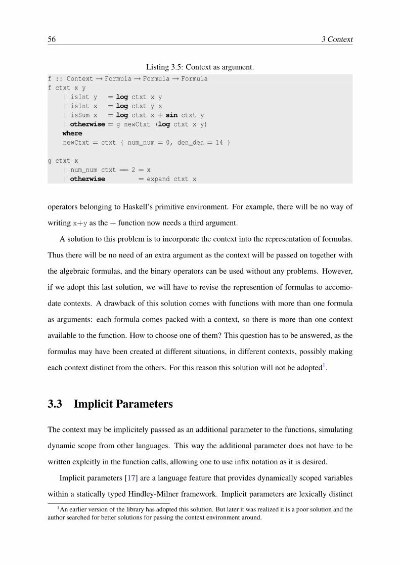
56 3 Context
Listing 3.5: Context as argument.f :: Context→ Formula→ Formula→ Formulaf ctxt x y
| isInt y = log ctxt x y| isInt x = log ctxt y x| isSum x = log ctxt x + sin ctxt y| otherwise = g newCtxt (log ctxt x y)wherenewCtxt = ctxt { num_num = 0, den_den = 14 }
g ctxt x| num_num ctxt == 2 = x| otherwise = expand ctxt x
operators belonging to Haskell’s primitive environment. For example, there will be no way of
writing x+y as the + function now needs a third argument.
A solution to this problem is to incorporate the context into the representation of formulas.
Thus there will be no need of an extra argument as the context will be passed on together with
the algebraic formulas, and the binary operators can be used without any problems. However,
if we adopt this last solution, we will have to revise the represention of formulas to accomo-
date contexts. A drawback of this solution comes with functions with more than one formula
as arguments: each formula comes packed with a context, so there is more than one context
available to the function. How to choose one of them? This question has to be answered, as the
formulas may have been created at different situations, in different contexts, possibly making
each context distinct from the others. For this reason this solution will not be adopted1.
3.3 Implicit Parameters
The context may be implicitely passsed as an additional parameter to the functions, simulating
dynamic scope from other languages. This way the additional parameter does not have to be
written explcitly in the function calls, allowing one to use infix notation as it is desired.
Implicit parameters [17] are a language feature that provides dynamically scoped variables
within a statically typed Hindley-Milner framework. Implicit parameters are lexically distinct
1An earlier version of the library has adopted this solution. But later it was realized it is a poor solution and theauthor searched for better solutions for passing the context environment around.
3.4 Alternative Solutions for Passing a Context Around 57
from regular identifiers, and are bound by a special with construct whose scope is dynamic,
rather static as with let. Implicit parameters are treated by the type system as parameters that
are not explicitly declared, but are inferred from their use.
Although Haskell 98 does not provide implicit parameters, most Haskell implementations
extend the language with this feautre, making it a feasable solution to the problem of passing
the context to function calls without explicitly adding a new parameter to them. Thus, we can
keep using binary operators to represent common binary arithmetic functions.
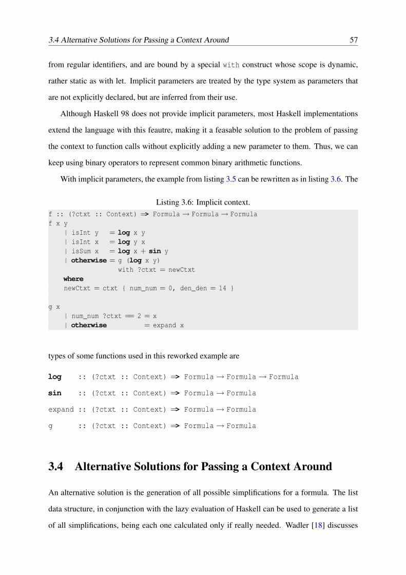
With implicit parameters, the example from listing 3.5 can be rewritten as in listing 3.6. The
Listing 3.6: Implicit context.f :: (?ctxt :: Context) => Formula→ Formula→ Formulaf x y
| isInt y = log x y| isInt x = log y x| isSum x = log x + sin y| otherwise = g (log x y)
types of some functions used in this reworked example are
log :: (?ctxt :: Context) => Formula→ Formula→ Formula
sin :: (?ctxt :: Context) => Formula→ Formula
expand :: (?ctxt :: Context) => Formula→ Formula
g :: (?ctxt :: Context) => Formula→ Formula
3.4 Alternative Solutions for Passing a Context Around
An alternative solution is the generation of all possible simplifications for a formula. The list
data structure, in conjunction with the lazy evaluation of Haskell can be used to generate a list
of all simplifications, being each one calculated only if really needed. Wadler [18] discusses
58 3 Context
backtracking in functional languages.
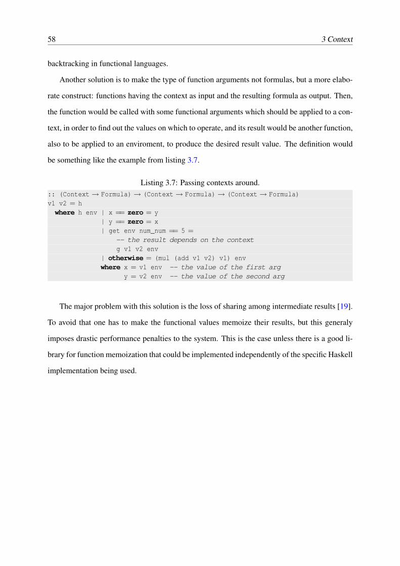
Another solution is to make the type of function arguments not formulas, but a more elabo-
rate construct: functions having the context as input and the resulting formula as output. Then,
the function would be called with some functional arguments which should be applied to a con-
text, in order to find out the values on which to operate, and its result would be another function,
also to be applied to an enviroment, to produce the desired result value. The definition would
be something like the example from listing 3.7.
Listing 3.7: Passing contexts around.:: (Context→ Formula)→ (Context→ Formula)→ (Context→ Formula)v1 v2 = hwhere h env | x == zero = y
| y == zero = x| get env num_num == 5 =
-- the result depends on the contextg v1 v2 env
| otherwise = (mul (add v1 v2) v1) envwhere x = v1 env -- the value of the first arg
y = v2 env -- the value of the second arg
The major problem with this solution is the loss of sharing among intermediate results [19].
To avoid that one has to make the functional values memoize their results, but this generaly
imposes drastic performance penalties to the system. This is the case unless there is a good li-
brary for function memoization that could be implemented independently of the specific Haskell
implementation being used.
Chapter 4Addition
In this chapter the algorithms employed to find the sum of any formulas are presented.
4.1 Basic Addition Rules
The addition of two arbitrary formulas may be reductible or not, depending on the formulas
being added. When it is reductible, the resulting sum is a formula computed by applying known
rules to the terms of the addition. For example, the sum of two rational numbers is a rational
number given by the rules for adding rational numbers, e.g.
34
+56
=
124×3+
126×5
12=
1912
But the addition may fail to produce a sum that is simpler than the stated addition. In this case
there is no option but to pack the terms being added in an application formula for sums. For
example, when adding an integer to a literal, e.g.
45+ x
there is no way to simplify the resulting sum and the result is left as an indication of the desired
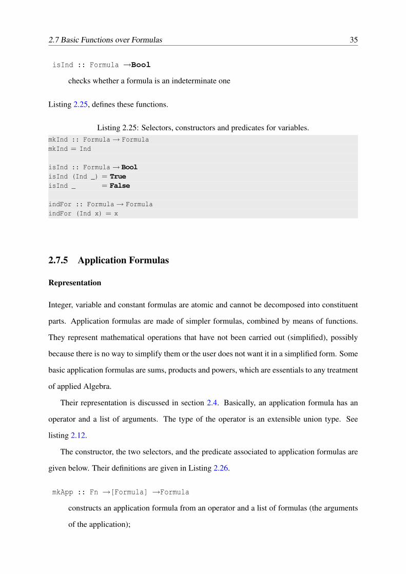
addition. Sections 2.1 and 2.7.5 discuss the representation of unreductible formulas, like the
one above.
59
60 4 Addition
The algorithms used to implement addition make use of a function that tries to add two
terms producing a reduced formula when it is possible, or an indication of failure when not. This
function handles the cases of addition to zero and addition of integers and rational numbers, with
the proviso of handling special cases when necessary. Section 2.9 discusses the representation
of success and failure by means of the Maybe data type.
4.2 Addition of Integer and Rational Numbers
The most basic rules handle addition of zero and any formula, and addition of integer and
rational numbers.
Zero is the identity value of the addition operation, so that
0+ x = x+0 = x
for any formula x.
Integer addition is carried out following the arithmetic rules taught at elementary levels of
Mathematics. The implementation makes use of the function
(+) :: Integer →Integer →Integer
from the standard library to handle it.
Mixed integer and rational addition is accomplished following the rule
n+pq
=n×q+ p
q
where n, p and q are integers and q > 0.
Rational addition is carried out by following the rule
mn
+pq
=m× k
n+ p× k
qk
4.3 Handling of Special Cases 61
where
k = lcm(n,q)
m, n, p and q are integer numbers, n > 0, q > 0 and lcm(n,q) is the least common multiple of
n and q. In the most general case the result is a rational number. When k = 1, the result is an
integer number.
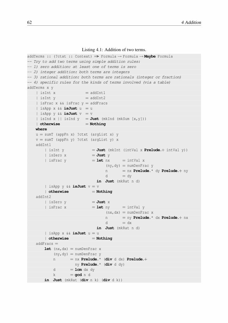
Listing 4.1 shows the implementation code for the basic rules discussed in the above sec-
tions.
4.3 Handling of Special Cases
Besides the basic rules for addition, it is possible to specify special rules. For example, there
is no provision for the addition of two logarithms in the core addition functions. How is it
supposed to be achieved? The library offers a mechanism to attach special rules for addition
into the algorithm that adds two formulas. The rules are triggered when none of the explicit
rules shown above is adequate to handle the addition. For this scheme to work, at least one of
the formulas being added must be an application formula.
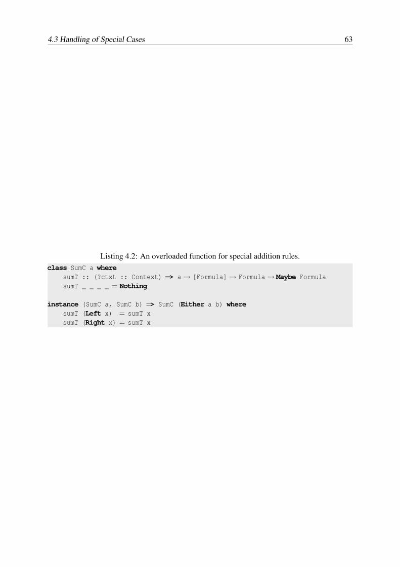
The core addition algorithm has a hook for calling customized functions when none of the
basic rules apply. The hook is an overloaded function called sumT, introduced by the class SumC
defined in listing 4.2. sumT is a function with three explicit arguments:
1. the operator of the application formula (the formula corresponding to the first formula to
be added),
2. the arguments of this application formula,
3. the second formula to be added.
The function may fail or succeed. If it succeeds the result is a formula corresponding to the
sum of the two argument formulas. This listing also declares an instance Either a b of class
SumC. This is important, as the type of the operator in application formulas is an extensible
62 4 Addition
Listing 4.1: Addition of two terms.addTerms :: (?ctxt :: Context) => Formula→ Formula→ Maybe Formula-- Try to add two terms using simple addition rules:-- 1) zero addition: at least one of terms is zero-- 2) integer addition: both terms are integers-- 3) rational addition: both terms are rationals (integer or fraction)-- 4) specific rules for the kinds of terms involved (via a table)addTerms x y
| isInt x = addInt1| isInt y = addInt2| isFrac x && isFrac y = addFracs| isApp x && isJust u = u| isApp y && isJust v = v| isInd x || isInd y = Just (mkInd (mkSum [x,y]))| otherwise = Nothingwhereu = sumT (appFn x) ?ctxt (argList x) yv = sumT (appFn y) ?ctxt (argList y) xaddInt1
| isInt y = Just (mkInt (intVal x Prelude.+ intVal y))| isZero x = Just y| isFrac y = let nx = intVal x
(ny,dy) = numDenFrac yn = nx Prelude.* dy Prelude.+ nyd = dy
in Just (mkRat n d)| isApp y && isJust v = v| otherwise = Nothing
addInt2| isZero y = Just x| isFrac x = let ny = intVal y
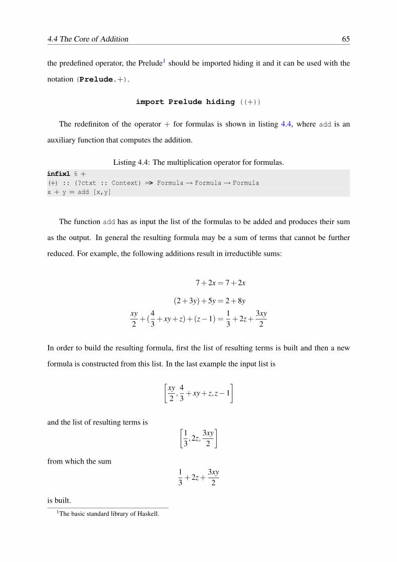
the predefined operator, the Prelude1 should be imported hiding it and it can be used with the
notation (Prelude.+).
import Prelude hiding ((+))
The redefiniton of the operator + for formulas is shown in listing 4.4, where add is an
auxiliary function that computes the addition.
Listing 4.4: The multiplication operator for formulas.infixl 6 +(+) :: (?ctxt :: Context) => Formula→ Formula→ Formulax + y = add [x,y]
The function add has as input the list of the formulas to be added and produces their sum
as the output. In general the resulting formula may be a sum of terms that cannot be further
reduced. For example, the following additions result in irreductible sums:
7+2x = 7+2x
(2+3y)+5y = 2+8y
xy2
+(43
+ xy+ z)+(z−1) =13
+2z+3xy2
In order to build the resulting formula, first the list of resulting terms is built and then a new
formula is constructed from this list. In the last example the input list is
[xy2
,43
+ xy+ z,z−1]
and the list of resulting terms is [13,2z,
3xy2
]from which the sum
13
+2z+3xy2
is built.1The basic standard library of Haskell.
66 4 Addition
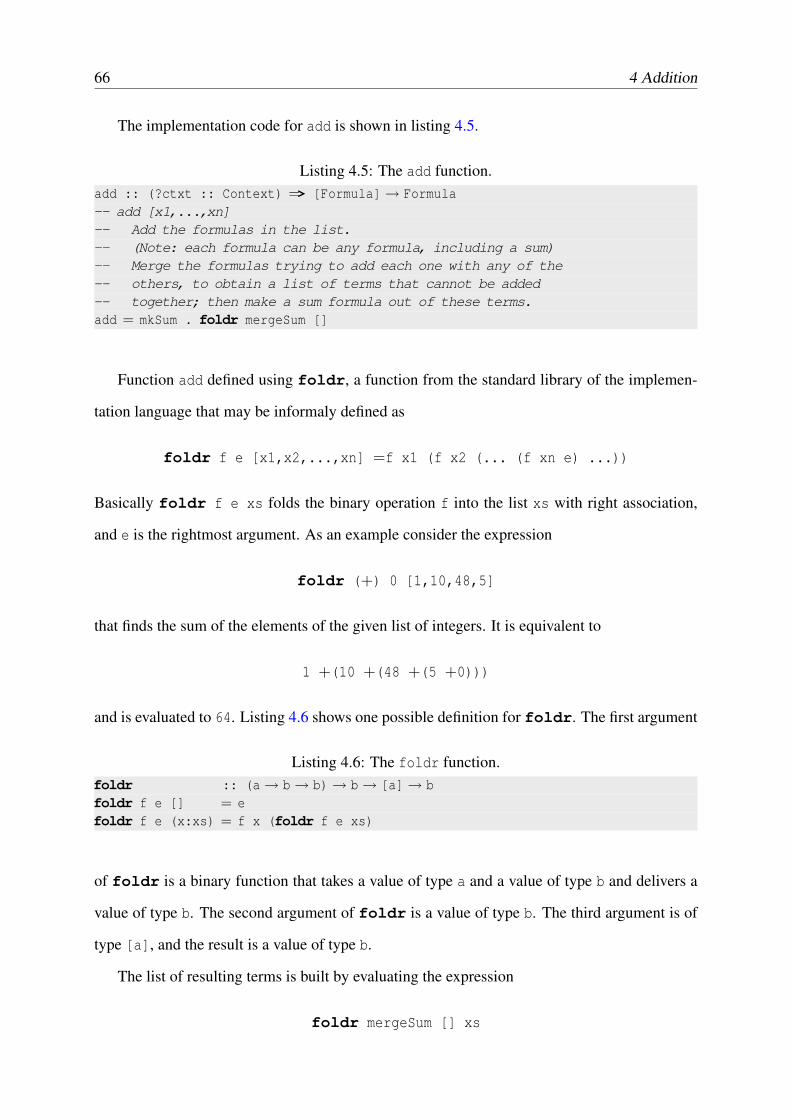
The implementation code for add is shown in listing 4.5.
Listing 4.5: The add function.add :: (?ctxt :: Context) => [Formula]→ Formula-- add [x1,...,xn]-- Add the formulas in the list.-- (Note: each formula can be any formula, including a sum)-- Merge the formulas trying to add each one with any of the-- others, to obtain a list of terms that cannot be added-- together; then make a sum formula out of these terms.add = mkSum . foldr mergeSum []
Function add defined using foldr, a function from the standard library of the implemen-
tation language that may be informaly defined as
foldr f e [x1,x2,...,xn] =f x1 (f x2 (... (f xn e) ...))
Basically foldr f e xs folds the binary operation f into the list xs with right association,
and e is the rightmost argument. As an example consider the expression
foldr (+) 0 [1,10,48,5]
that finds the sum of the elements of the given list of integers. It is equivalent to
1 +(10 +(48 +(5 +0)))
and is evaluated to 64. Listing 4.6 shows one possible definition for foldr. The first argument
Listing 4.6: The foldr function.foldr :: (a→ b→ b)→ b→ [a]→ bfoldr f e [] = efoldr f e (x:xs) = f x (foldr f e xs)
of foldr is a binary function that takes a value of type a and a value of type b and delivers a
value of type b. The second argument of foldr is a value of type b. The third argument is of
type [a], and the result is a value of type b.
The list of resulting terms is built by evaluating the expression
foldr mergeSum [] xs
4.4 The Core of Addition 67
(from the definition of add). If xs =[x0,x1,...,xn], it is equivalent to
mergeSum works with two arguments. Its first argument x is a term from the addition that is
being carried out. The second argument ys is a list of the terms of the sum that will be the result
of the addition, which has been partially built so far. mergeSum checks if x is a sum or not. If x
is a sum x1 + x2 + . . .+ xn then it should be split in its constituent terms x1, x2, . . . , xn and each
term should be dealt separately. Otherwise it is dealt as a single term x. Each term taken from x
in this way is then merged with the terms in ys:
• if ys is the empty list then the result is the list of terms from x, that is, [x] if x is not a sum
or [x1,x2, . . . ,xn] if x is the sum x1 + x2 + . . .+ xn.
• if ys is not empty then the result is obtained by combining each term from x, that is, x
itself if it is not a sum, or x1, x2, . . . , xn if x is the sum x1 + x2 + . . .+ xn, with the list ys
using the function mergeTerm that is discussed in the sequence. This is accomplished by
evaluating the expression
mergeTerm x ys
in the first case, and
4.4 The Core of Addition 69
foldr mergeTerm ys [x1,x2,...,xn]
in the second case.
Listing 4.7 shows the implementation of mergeSum.
Listing 4.7: The mergeSum function.mergeSum :: (?ctxt :: Context) => Formula→ [Formula]→ [Formula]-- mergeSum x ys-- ys is a list [y1, y2, ..., yn] of formulas whose sum-- y1 + y2 + ... + yn-- cannot be simplified in the current context.-- xs is a formula, possibly a sum, to be added to the formula-- y1 + y2 + ... + yn-- whose terms are the elements of ys.-- Basicaly there is a check whether x is a sum. In this case-- its terms should be merged with ys, one at a time.-- Otherwise x should be merged directly with ys.mergeSum x []
| isSum x = appArgs x| otherwise = [x]
mergeSum x ys| isSum x = foldr mergeTerm ys (appArgs x)| otherwise = mergeTerm x ys
As examples of how mergeSum simplifies consider the following reductions:
mergeSum (5x) []
= [5x]
mergeSum (2+x+3y) []
= [2,x,3y]
mergeSum (5x) [7,x,3y]
= mergeTerm (5x) [7,x,3y]
= [7,6x,3y]
mergeSum (2+x+3y) [7,x,3y]
= foldr mergeTerm [7,x,3y] [2,x,3y]
70 4 Addition
= mergeTerm 2 (mergeTerm x (mergeTerm (3y) [7,x,3y]))
= mergeTerm 2 (mergeTerm x [7,x,6y])
= mergeTerm 2 [7,2x,6y]
= [9,2x,6y]
mergeTerm is applied to two arguments. The first argument x is a formula (but it is not
a sum) that must be added to the sum of the formulas that appear as the second argument
ys = [y1,y2, . . . ,yn], a list of terms. So the expression mergeTerm (2x) [5,8x,3y] finds the
sum (2x) +(5+8x+3y). The algorithm for mergeTerm has its fundaments in the comutative
and associative laws of addition. It has three phases:
1. An attempt is made to add x to one of the the terms yi in ys. Each term yi in ys is tried out
starting with i = 1 until the x and yi can be successfuly added using addTerms. In this
case the result is given by combining the sum x+ yi computed by addTerms with the list
of terms that is obtained by dropping yi from ys, that is, [y1, . . . ,yi−1,yi+1, . . . ,yn] using
mergeSum. If there is no yi such that x and yi could be added using addTerms then the
second phase starts.
2. Two terms x and y with a common literal part can be added by adding their coefficients.
So if x = cxlx and y = cyly where cx and lx are respectively the coefficient and literal part
of x and cy and ly are respectively the coefficient and literal part of y and lx = ly = l then
the sum can be computed as
x+ y = cxlx + cyly = (cx + cy)l
In this phase a term yi from the list ys with the same literal part l of x is searched for by
starting with i = 1. If found the result is obtained by replacing yi with the sum of x and yi
computed as explained above in the list ys, if the sum is not equal to 0, in which case yi
is simply removed from ys. If there is no yi in ys with the same literal part as x then starts
the third phase.
3. In this phase x will be inserted into ys to build the result, as there is no way to merge it
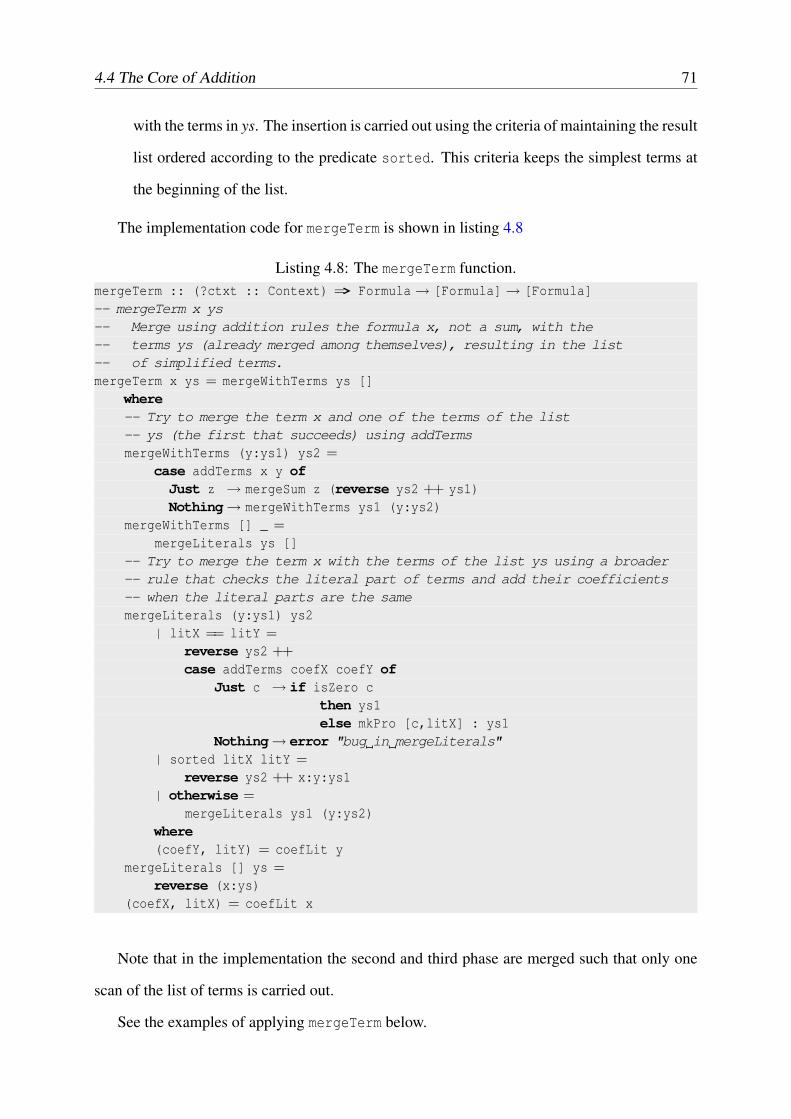
4.4 The Core of Addition 71
with the terms in ys. The insertion is carried out using the criteria of maintaining the result
list ordered according to the predicate sorted. This criteria keeps the simplest terms at
the beginning of the list.
The implementation code for mergeTerm is shown in listing 4.8
Listing 4.8: The mergeTerm function.mergeTerm :: (?ctxt :: Context) => Formula→ [Formula]→ [Formula]-- mergeTerm x ys-- Merge using addition rules the formula x, not a sum, with the-- terms ys (already merged among themselves), resulting in the list-- of simplified terms.mergeTerm x ys = mergeWithTerms ys []
where-- Try to merge the term x and one of the terms of the list-- ys (the first that succeeds) using addTermsmergeWithTerms (y:ys1) ys2 =
case addTerms x y ofJust z → mergeSum z (reverse ys2 ++ ys1)Nothing→ mergeWithTerms ys1 (y:ys2)
mergeWithTerms [] _ =mergeLiterals ys []
-- Try to merge the term x with the terms of the list ys using a broader-- rule that checks the literal part of terms and add their coefficients-- when the literal parts are the samemergeLiterals (y:ys1) ys2
Just c → if isZero cthen ys1else mkPro [c,litX] : ys1
Nothing→ error "bug in mergeLiterals"| sorted litX litY =
reverse ys2 ++ x:y:ys1| otherwise =
mergeLiterals ys1 (y:ys2)where(coefY, litY) = coefLit y
mergeLiterals [] ys =reverse (x:ys)
(coefX, litX) = coefLit x
Note that in the implementation the second and third phase are merged such that only one
scan of the list of terms is carried out.
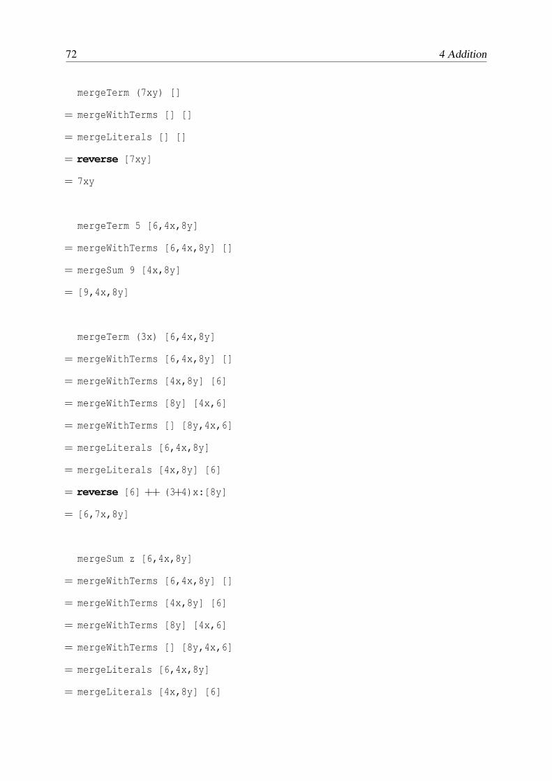
See the examples of applying mergeTerm below.
72 4 Addition
mergeTerm (7xy) []
= mergeWithTerms [] []
= mergeLiterals [] []
= reverse [7xy]
= 7xy
mergeTerm 5 [6,4x,8y]
= mergeWithTerms [6,4x,8y] []
= mergeSum 9 [4x,8y]
= [9,4x,8y]
mergeTerm (3x) [6,4x,8y]
= mergeWithTerms [6,4x,8y] []
= mergeWithTerms [4x,8y] [6]
= mergeWithTerms [8y] [4x,6]
= mergeWithTerms [] [8y,4x,6]
= mergeLiterals [6,4x,8y]
= mergeLiterals [4x,8y] [6]
= reverse [6] ++ (3+4)x:[8y]
= [6,7x,8y]
mergeSum z [6,4x,8y]
= mergeWithTerms [6,4x,8y] []
= mergeWithTerms [4x,8y] [6]
= mergeWithTerms [8y] [4x,6]
= mergeWithTerms [] [8y,4x,6]
= mergeLiterals [6,4x,8y]
= mergeLiterals [4x,8y] [6]
4.4 The Core of Addition 73
= mergeLiterals [8y] [4x,6]
= mergeLiterals [] [8y,4x,6]
= reverse (z:[8y,4x,6])
= [6,4x,8y,z]
Chapter 5Multiplication and Subtraction
In this chapter, the author presents the algorithms employed to find the product and the differ-
ence of formulas. The framework of the multiplication algorithms follows the general guide-
lines presented for addition. However, specific multiplication rules replaces those for addition.
Therefore, one is advised to brush up on his/her knowledge of addition before reading this
chapter.
5.1 Basic Multiplication Rules
Like addition, the multiplication of two arbitrary formulas may be reductible or not, depending
on the formulas being multiplied. When it is reductible, the resulting product is a formula
computed applying known rules to the factors of the multiplication. For example, the product
of two rational numbers is a rational number given by the rules for multiplying rational numbers,
e.g.34× 5
6=
3×54×6
=1230
=25
But the multiplication algorithm may fail in producing a product that is simpler than the stated
multiplication. In this case there is no option unless to pack the factors being multiplied in an
application formula for products. For example, when multiplying an integer and a literal, e.g.
5×a
74
5.2 Multiplication of Integers 75
there is no way to simplify the resulting product and the result is left as an indication of the de-
sired multiplication. Sections 2.1 and 2.7.5 discuss the representation of unreductible formulas,
like the one above.
The algorithms used to implement multiplication makes use of a function that tries to mul-
tiply two factors producing a reduced formula when possible, or an indication of failure other-
wise. This function handles the cases of multiplication by zero, by one, and multiplication of
integers, and makes proviso for the handling of special cases when necessary.
5.2 Multiplication of Integers
The most basic rules deal with multiplication by zero, by one, and multiplication of integer
numbers.
Zero is the zero value of the multiplication operation, that is
0× x = x×0 = 0
for any formula x.
One is the unit value of the multiplication operation, so
1× x = x×1 = x
for any formula x.
Integer multiplication is carried out following rules from elementary school Arithmetics.
The implementation makes use of the function
(*) :: Integer →Integer →Integer
which is taken from the standard library.
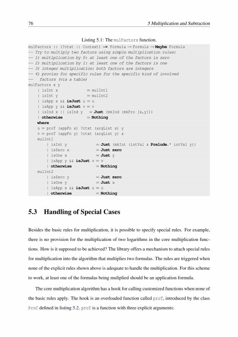
Listing 5.1 shows the implementation code for the basic rules discussed in the above sec-
tions.
76 5 Multiplication and Subtraction
Listing 5.1: The mulFactors function.mulFactors :: (?ctxt :: Context) => Formula→ Formula→ Maybe Formula-- Try to multiply two factors using simple multiplication rules:-- 1) multiplication by 0: at least one of the factors is zero-- 2) multiplication by 1: at least one of the factors is one-- 3) integer multiplication: both factors are integers-- 4) proviso for specific rules for the specific kind of involved-- factors (via a table)mulFactors x y
| isInt x = mulInt1| isInt y = mulInt2| isApp x && isJust u = u| isApp y && isJust v = v| isInd x || isInd y = Just (mkInd (mkPro [x,y]))| otherwise = Nothingwhereu = proT (appFn x) ?ctxt (argList x) yv = proT (appFn y) ?ctxt (argList y) xmulInt1
| isInt y = Just (mkInt (intVal x Prelude.* intVal y))| isZero x = Just zero| isOne x = Just y| isApp y && isJust v = v| otherwise = Nothing
mulInt2| isZero y = Just zero| isOne y = Just x| isApp x && isJust u = u| otherwise = Nothing
5.3 Handling of Special Cases
Besides the basic rules for multiplication, it is possible to specify special rules. For example,
there is no provision for the multiplication of two logarithms in the core multiplication func-
tions. How is it supposed to be achieved? The library offers a mechanism to attach special rules
for multiplication into the algorithm that multiplies two formulas. The rules are triggered when
none of the explicit rules shown above is adequate to handle the multiplication. For this scheme
to work, at least one of the formulas being muliplied should be an application formula.
The core multiplication algorithm has a hook for calling customized functions when none of
the basic rules apply. The hook is an overloaded function called proT, introduced by the class
ProC defined in listing 5.2. proT is a function with three explicit arguments:
5.3 Handling of Special Cases 77
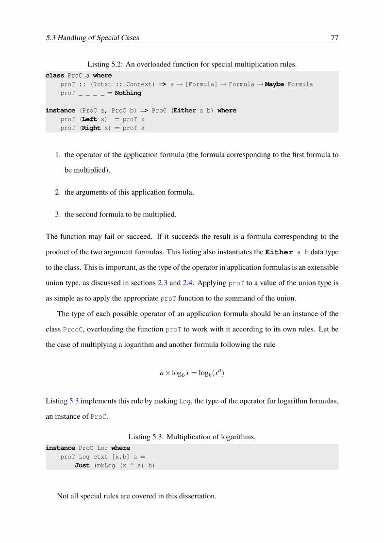
Listing 5.2: An overloaded function for special multiplication rules.class ProC a where
instance (ProC a, ProC b) => ProC (Either a b) whereproT (Left x) = proT xproT (Right x) = proT x
1. the operator of the application formula (the formula corresponding to the first formula to
be multiplied),
2. the arguments of this application formula,
3. the second formula to be multiplied.
The function may fail or succeed. If it succeeds the result is a formula corresponding to the
product of the two argument formulas. This listing also instantiates the Either a b data type
to the class. This is important, as the type of the operator in application formulas is an extensible
union type, as discussed in sections 2.3 and 2.4. Applying proT to a value of the union type is
as simple as to apply the appropriate proT function to the summand of the union.
The type of each possible operator of an application formula should be an instance of the
class ProcC, overloading the function proT to work with it according to its own rules. Let be
the case of multiplying a logarithm and another formula following the rule
a× logb x = logb(xa)
Listing 5.3 implements this rule by making Log, the type of the operator for logarithm formulas,
an instance of ProC.
Listing 5.3: Multiplication of logarithms.instance ProC Log where
proT Log ctxt [x,b] a =Just (mkLog (x ^ a) b)
Not all special rules are covered in this dissertation.
78 5 Multiplication and Subtraction
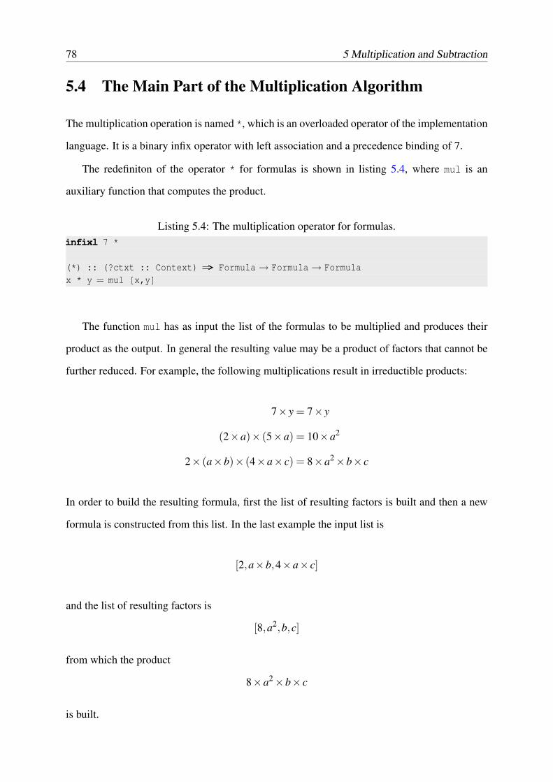
5.4 The Main Part of the Multiplication Algorithm
The multiplication operation is named *, which is an overloaded operator of the implementation
language. It is a binary infix operator with left association and a precedence binding of 7.
The redefiniton of the operator * for formulas is shown in listing 5.4, where mul is an
auxiliary function that computes the product.
Listing 5.4: The multiplication operator for formulas.infixl 7 *
(*) :: (?ctxt :: Context) => Formula→ Formula→ Formulax * y = mul [x,y]
The function mul has as input the list of the formulas to be multiplied and produces their
product as the output. In general the resulting value may be a product of factors that cannot be
further reduced. For example, the following multiplications result in irreductible products:
7× y = 7× y
(2×a)× (5×a) = 10×a2
2× (a×b)× (4×a× c) = 8×a2×b× c
In order to build the resulting formula, first the list of resulting factors is built and then a new
formula is constructed from this list. In the last example the input list is
[2,a×b,4×a× c]
and the list of resulting factors is
[8,a2,b,c]
from which the product
8×a2×b× c
is built.
5.4 The Main Part of the Multiplication Algorithm 79
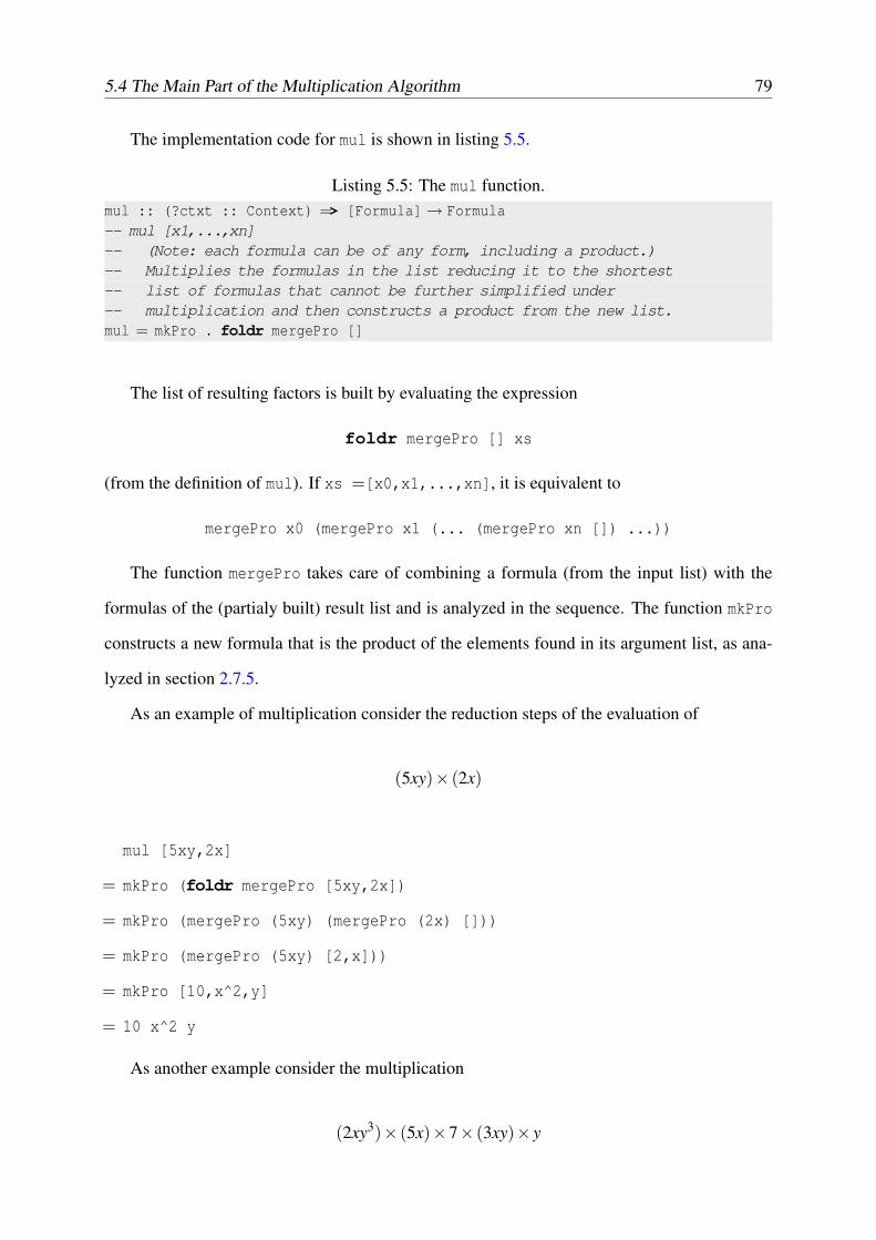
The implementation code for mul is shown in listing 5.5.
Listing 5.5: The mul function.mul :: (?ctxt :: Context) => [Formula]→ Formula-- mul [x1,...,xn]-- (Note: each formula can be of any form, including a product.)-- Multiplies the formulas in the list reducing it to the shortest-- list of formulas that cannot be further simplified under-- multiplication and then constructs a product from the new list.mul = mkPro . foldr mergePro []
The list of resulting factors is built by evaluating the expression
foldr mergePro [] xs
(from the definition of mul). If xs =[x0,x1,...,xn], it is equivalent to
The function mergePro takes care of combining a formula (from the input list) with the
formulas of the (partialy built) result list and is analyzed in the sequence. The function mkPro
constructs a new formula that is the product of the elements found in its argument list, as ana-
lyzed in section 2.7.5.
As an example of multiplication consider the reduction steps of the evaluation of
(5xy)× (2x)
mul [5xy,2x]
= mkPro (foldr mergePro [5xy,2x])
= mkPro (mergePro (5xy) (mergePro (2x) []))
= mkPro (mergePro (5xy) [2,x]))
= mkPro [10,x^2,y]
= 10 x^2 y
As another example consider the multiplication
(2xy3)× (5x)×7× (3xy)× y
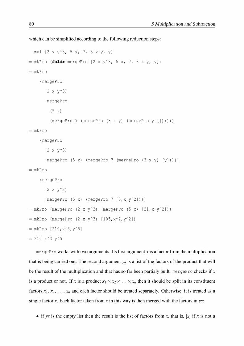
80 5 Multiplication and Subtraction
which can be simplified according to the following reduction steps:
mul [2 x y^3, 5 x, 7, 3 x y, y]
= mkPro (foldr mergePro [2 x y^3, 5 x, 7, 3 x y, y])
= mkPro
(mergePro
(2 x y^3)
(mergePro
(5 x)
(mergePro 7 (mergePro (3 x y) (mergePro y [])))))
= mkPro
(mergePro
(2 x y^3)
(mergePro (5 x) (mergePro 7 (mergePro (3 x y) [y]))))
= mkPro
(mergePro
(2 x y^3)
(mergePro (5 x) (mergePro 7 [3,x,y^2])))
= mkPro (mergePro (2 x y^3) (mergePro (5 x) [21,x,y^2]))
= mkPro (mergePro (2 x y^3) [105,x^2,y^2])
= mkPro [210,x^3,y^5]
= 210 x^3 y^5
mergePro works with two arguments. Its first argument x is a factor from the multiplication
that is being carried out. The second argument ys is a list of the factors of the product that will
be the result of the multiplication and that has so far been partialy built. mergePro checks if x
is a product or not. If x is a product x1× x2× . . .× xn then it should be split in its constituent
factors x1, x2, . . . , xn and each factor should be treated separately. Otherwise, it is treated as a
single factor x. Each factor taken from x in this way is then merged with the factors in ys:
• if ys is the empty list then the result is the list of factors from x, that is, [x] if x is not a
5.4 The Main Part of the Multiplication Algorithm 81
product or [x1,x2, . . . ,xn] if x is the product x1× x2× . . .× xn.
• if ys is not empty then the result is obtained by combining each factor from x, that is, x
itself if it is not a product, or x1, x2, . . . , xn if x is the product x1×x2× . . .×xn, with the list
ys using the function mergeFactor that is analyzed in the sequence. This is accomplished
by evaluating the expression
mergeFactor x ys
in the first case, and
foldr mergeFactor ys [x1,x2,...,xn]
in the second case.
The implementation of mergePro follows in listing 5.6.
Listing 5.6: The mergePro function.mergePro :: (?ctxt :: Context) => Formula→ [Formula]→ [Formula]-- mergePro x ys-- ys is a list [y1, y2, ..., yn] of formulas whose product-- y1 * y2 * ... * yn-- cannot be simplified in the current context.-- xs is a formula, possibly a product, to be multiplied-- with the formula-- y1 * y2 * ... * yn-- whose factors are the elements of ys.-- Basicaly there is a check whether x is a product. In this-- case its factors should be merged with ys, one at a time.-- Otherwise x should be merged directly with ys.mergePro x []
| isPro x = appArgs x| otherwise = [x]
mergePro x ys| isPro x = foldr mergeFactor ys (appArgs x)| otherwise = mergeFactor x ys
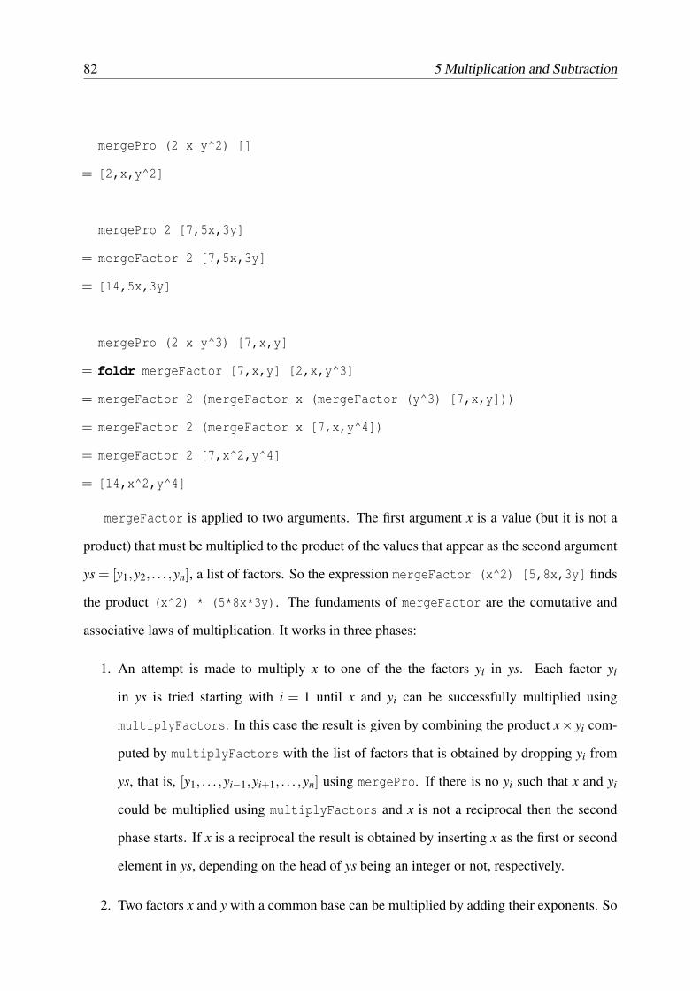
As examples of how mergePro simplifies expressions, consider the following reductions:
mergePro (2+x) []
= [2+x]
82 5 Multiplication and Subtraction
mergePro (2 x y^2) []
= [2,x,y^2]
mergePro 2 [7,5x,3y]
= mergeFactor 2 [7,5x,3y]
= [14,5x,3y]
mergePro (2 x y^3) [7,x,y]
= foldr mergeFactor [7,x,y] [2,x,y^3]
= mergeFactor 2 (mergeFactor x (mergeFactor (y^3) [7,x,y]))
= mergeFactor 2 (mergeFactor x [7,x,y^4])
= mergeFactor 2 [7,x^2,y^4]
= [14,x^2,y^4]
mergeFactor is applied to two arguments. The first argument x is a value (but it is not a
product) that must be multiplied to the product of the values that appear as the second argument
ys = [y1,y2, . . . ,yn], a list of factors. So the expression mergeFactor (x^2) [5,8x,3y] finds
the product (x^2) * (5*8x*3y). The fundaments of mergeFactor are the comutative and
associative laws of multiplication. It works in three phases:
1. An attempt is made to multiply x to one of the the factors yi in ys. Each factor yi
in ys is tried starting with i = 1 until x and yi can be successfully multiplied using
multiplyFactors. In this case the result is given by combining the product x× yi com-
puted by multiplyFactors with the list of factors that is obtained by dropping yi from
ys, that is, [y1, . . . ,yi−1,yi+1, . . . ,yn] using mergePro. If there is no yi such that x and yi
could be multiplied using multiplyFactors and x is not a reciprocal then the second
phase starts. If x is a reciprocal the result is obtained by inserting x as the first or second
element in ys, depending on the head of ys being an integer or not, respectively.
2. Two factors x and y with a common base can be multiplied by adding their exponents. So
5.4 The Main Part of the Multiplication Algorithm 83
if x = bxex and y = by
ey where bx and ex are respectively the base and the exponent of x
and by and ey are respectively the base and the exponent of y and bx = by = b then the
product can be computed as
x× y = bxex ×by
ey = bex+ey
In this phase a factor yi from the list ys with the same base b of x is searched for starting
with i = 1. If found the result is obtained by replacing yi with the product of x and yi
computed as explained above in the list ys. If there is no yi in ys with the same base as x
then starts the third phase.
3. In this phase x will be inserted into ys to build the result, as there is no way of combining
it with the factors in ys. The insertion is carried out using the criteria of maintaining the
result list ordered according to the precedence of formulas (section 2.8) and keeping num-
bers at the beginning of the list. This criteria keeps the simplest factors at the beginning
of the list.
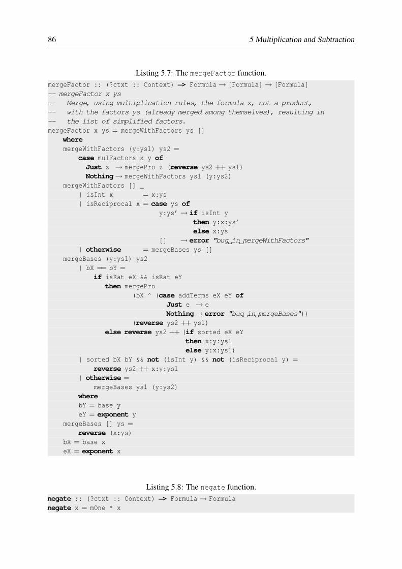
Listing 5.7 presents the implementation code for mergeFactor.
Note that in the implementation the second and third phases are merged such that, only one
scan of the list of factors is completed.
See the examples of applying mergeFactor in the sequence.
mergeFactor (a+b) []
= mergeWithFactors [] []
= mergeBases [] []
= reverse [a+b]
= a+b
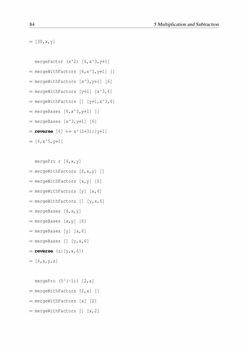
mergeFactor 5 [6,x,y]
= mergeWithFactors [6,x,y] []
= mergePro 30 [x,y]
84 5 Multiplication and Subtraction
= [30,x,y]
mergeFactor (x^2) [6,x^3,y+1]
= mergeWithFactors [6,x^3,y+1] []
= mergeWithFactors [x^3,y+1] [6]
= mergeWithFactors [y+1] [x^3,6]
= mergeWithFactors [] [y+1,x^3,6]
= mergeBases [6,x^3,y+1] []
= mergeBases [x^3,y+1] [6]
= reverse [6] ++ x^(2+3):[y+1]
= [6,x^5,y+1]
mergePro z [6,x,y]
= mergeWithFactors [6,x,y] []
= mergeWithFactors [x,y] [6]
= mergeWithFactors [y] [x,6]
= mergeWithFactors [] [y,x,6]
= mergeBases [6,x,y]
= mergeBases [x,y] [6]
= mergeBases [y] [x,6]
= mergeBases [] [y,x,6]
= reverse (z:[y,x,6])
= [6,x,y,z]
mergePro (5^(-1)) [2,x]
= mergeWithFactors [2,x] []
= mergeWithFactors [x] [2]
= mergeWithFactors [] [x,2]
5.5 Additive Inverse and Subtraction 85
= [2,5^(-1),x]
5.5 Additive Inverse and Subtraction
The additive inverse of a number x is defined as the product of −1 and x. Our implementation
language provides an overloaded identifier named negate for the additive inverse functions.
The library redefines it to invert formulas, as shown in listing 5.8.
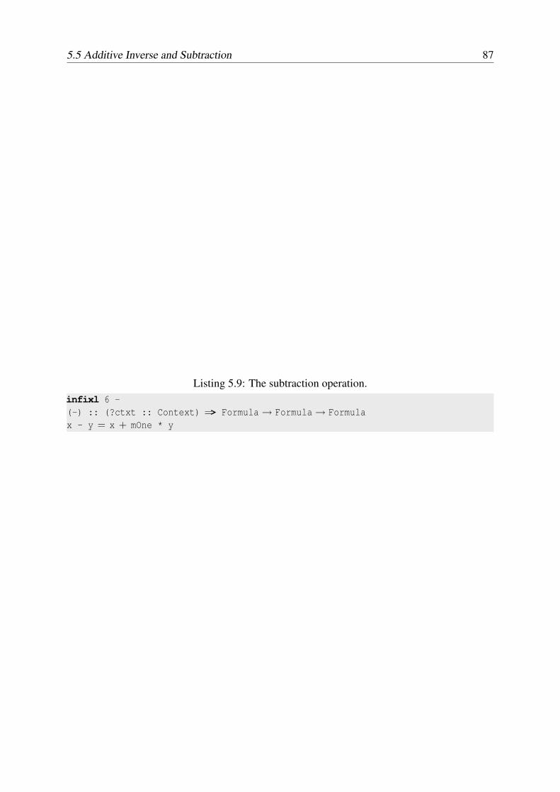
The subtraction operation is named -, and overloaded infix operator of the implementation
language. This operator is non associative and has precedence 6. It is also redefine to calculate
the difference of two formulas. Listing 5.9 shows its new definition, based on the rule
x− y = x× (−y)
86 5 Multiplication and Subtraction
Listing 5.7: The mergeFactor function.mergeFactor :: (?ctxt :: Context) => Formula→ [Formula]→ [Formula]-- mergeFactor x ys-- Merge, using multiplication rules, the formula x, not a product,-- with the factors ys (already merged among themselves), resulting in-- the list of simplified factors.mergeFactor x ys = mergeWithFactors ys []
wheremergeWithFactors (y:ys1) ys2 =
case mulFactors x y ofJust z → mergePro z (reverse ys2 ++ ys1)Nothing→ mergeWithFactors ys1 (y:ys2)
mergeWithFactors [] _| isInt x = x:ys| isReciprocal x = case ys of
instance (BaseC a, BaseC b) => BaseC (Either a b) wherebaseT (Left x) = baseT xbaseT (Right x) = baseT x
class ExponentC a whereexponentT :: (?ctxt :: Context) => a→ Formula→ [Formula]→ Maybe FormulaexponentT _ _ _ _ = Nothing
instance (ExponentC a, ExponentC b) => ExponentC (Either a b) whereexponentT (Left x) = exponentT xexponentT (Right x) = exponentT x
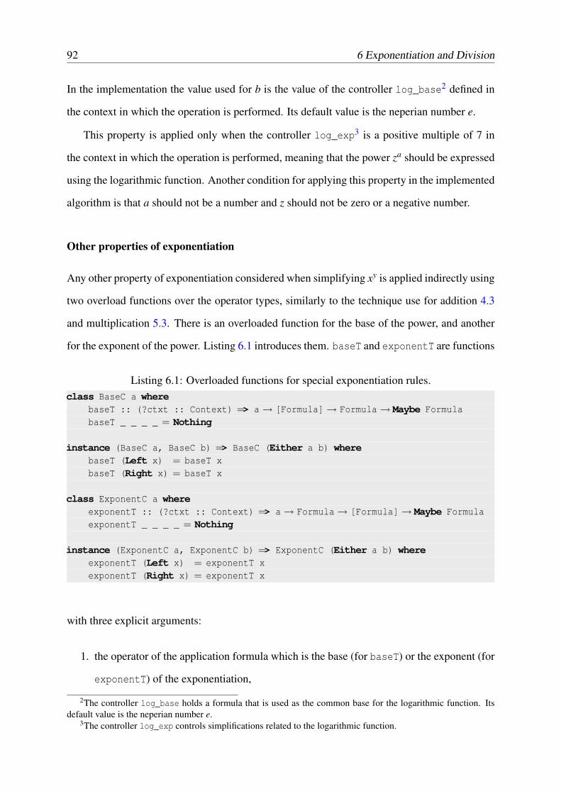
with three explicit arguments:
1. the operator of the application formula which is the base (for baseT) or the exponent (for
exponentT) of the exponentiation,
2The controller log_base holds a formula that is used as the common base for the logarithmic function. Itsdefault value is the neperian number e.
3The controller log_exp controls simplifications related to the logarithmic function.
6.3 Special properties of exponentiation 93
2. the arguments of this application formula,
3. the second formula, which is the exponent (for baseT) or the base (for exponentT).
The functions may fail or succeed. If baseT succeeds the result is a formula corresponding
to the power of the first formula to the second formula. If exponentT succeeds the result is
a formula corresponding to the power of the second formula to the first formula. This listing
also instantiates the Either a b data type to the classes. This is important, as the type of the
operator in application formulas is an extensible union type, as discussed in sections 2.3 and
2.4. Applying baseT or exponentT to a value of the union type is as simple as to apply the
appropriate proT or exponentT function to the summand of the union.
Non simplifiable powers
When it is not possible to simplify a power, the result will be a new formula representing the
exponentiation operation, built using the function mkPow.
Implementation code
Listings 6.2 – 6.7 shows the code that implements these basic properties of exponentiation.
6.3 Special properties of exponentiation
Product where a factor is a power
This rule will be triggered when simplifying a product and one of the factors is a power.
x · ya
Two cases of simplification are handled here. Other cases of products where a factor is a power
are not handled at this point.
94 6 Exponentiation and Division
Listing 6.2: Power of two terms.infixr 8 ^(^) :: (?ctxt :: Context) => Formula→ Formula→ Formulax ^ y
| isInt y = powAnyInt x (intVal y)| isOne x = one| isZero x = powZeroAny y| isE x && isI y &&
negMult (trig_expd ?ctxt) 7 = cos one + i * sin one| x /= logBase &¬ (less x zero) &¬ (isRat x) &&posMult (log_expd ?ctxt) 7 = logBase ^ y * log x logBase
| isApp x && isJust u = fromJust u| isApp y && isJust v = fromJust v| isInd x || isInd y = mkInd (mkPow x y)| otherwise = mkPow x ywherelogBase = log_base ?ctxtu = baseT (appFn x) ?ctxt (arguments x) yv = exponentT (appFn y) ?ctxt x (arguments y)
Division of two integers. The division of two integer numbers x and y is handled by building a
fraction xy followed by its simplification. The result may be an integer, a reciprocal or a fraction.
x · y−1 = x · 1y
=xy
=
xmym
where
m = gcd(x,y)
Listing 6.3: Power of two terms (continued).powAnyInt x yVal
Listing 6.5: Power of two terms (continued).powZeroAny y
| less y zero = mkInd (mkPow zero y)| greater y zero = zero| zero_base ?ctxt = zero| otherwise = mkPow zero y
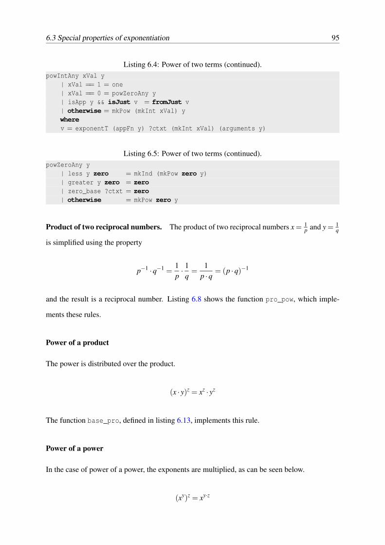
Product of two reciprocal numbers. The product of two reciprocal numbers x = 1p and y = 1
q
is simplified using the property
p−1 ·q−1 =1p· 1
q=
1p ·q
= (p ·q)−1
and the result is a reciprocal number. Listing 6.8 shows the function pro_pow, which imple-
ments these rules.
Power of a product
The power is distributed over the product.
(x · y)z = xz · yz
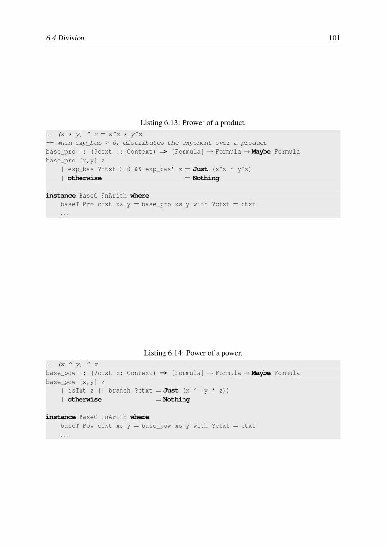
The function base_pro, defined in listing 6.13, implements this rule.
Power of a power
In the case of power of a power, the exponents are multiplied, as can be seen below.
(xy)z = xy·z
96 6 Exponentiation and Division
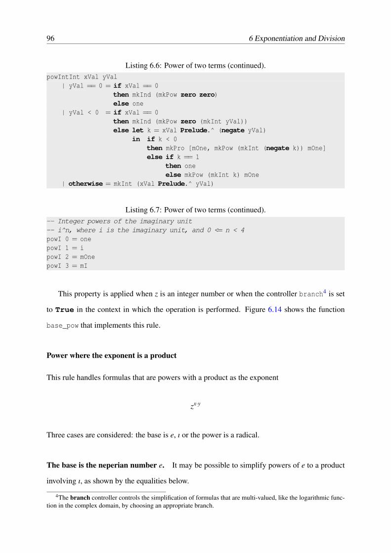
Listing 6.6: Power of two terms (continued).powIntInt xVal yVal
| yVal == 0 = if xVal == 0then mkInd (mkPow zero zero)else one
| yVal < 0 = if xVal == 0then mkInd (mkPow zero (mkInt yVal))else let k = xVal Prelude.^ (negate yVal)
in if k < 0then mkPro [mOne, mkPow (mkInt (negate k)) mOne]else if k == 1
then oneelse mkPow (mkInt k) mOne
| otherwise = mkInt (xVal Prelude.^ yVal)
Listing 6.7: Power of two terms (continued).-- Integer powers of the imaginary unit-- i^n, where i is the imaginary unit, and 0 <= n < 4powI 0 = onepowI 1 = ipowI 2 = mOnepowI 3 = mI
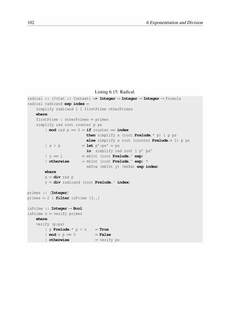
This property is applied when z is an integer number or when the controller branch4 is set
to True in the context in which the operation is performed. Figure 6.14 shows the function
base_pow that implements this rule.
Power where the exponent is a product
This rule handles formulas that are powers with a product as the exponent
zx·y
Three cases are considered: the base is e, ı or the power is a radical.
The base is the neperian number e. It may be possible to simplify powers of e to a product
involving ı, as shown by the equalities below.
4The branch controller controls the simplification of formulas that are multi-valued, like the logarithmic func-tion in the complex domain, by choosing an appropriate branch.
6.3 Special properties of exponentiation 97
Listing 6.8: Product of power.-- x * (y ^ a)-- (y^n) * (y^a) = y (n+a) when bas_exp < 0 && bas_exp’ y-- (k^a) * (y^a) = (k*y) a when exp_bas < 0 && exp_bas’ a-- x * (y -1) = x/y
The use of the third property is controlled by the trig_exp controller setting in the context
in which the simplification is performed. Exponentials are converted to trigonometric functions
only when trig_exp is a negative multiple of 7.
98 6 Exponentiation and Division
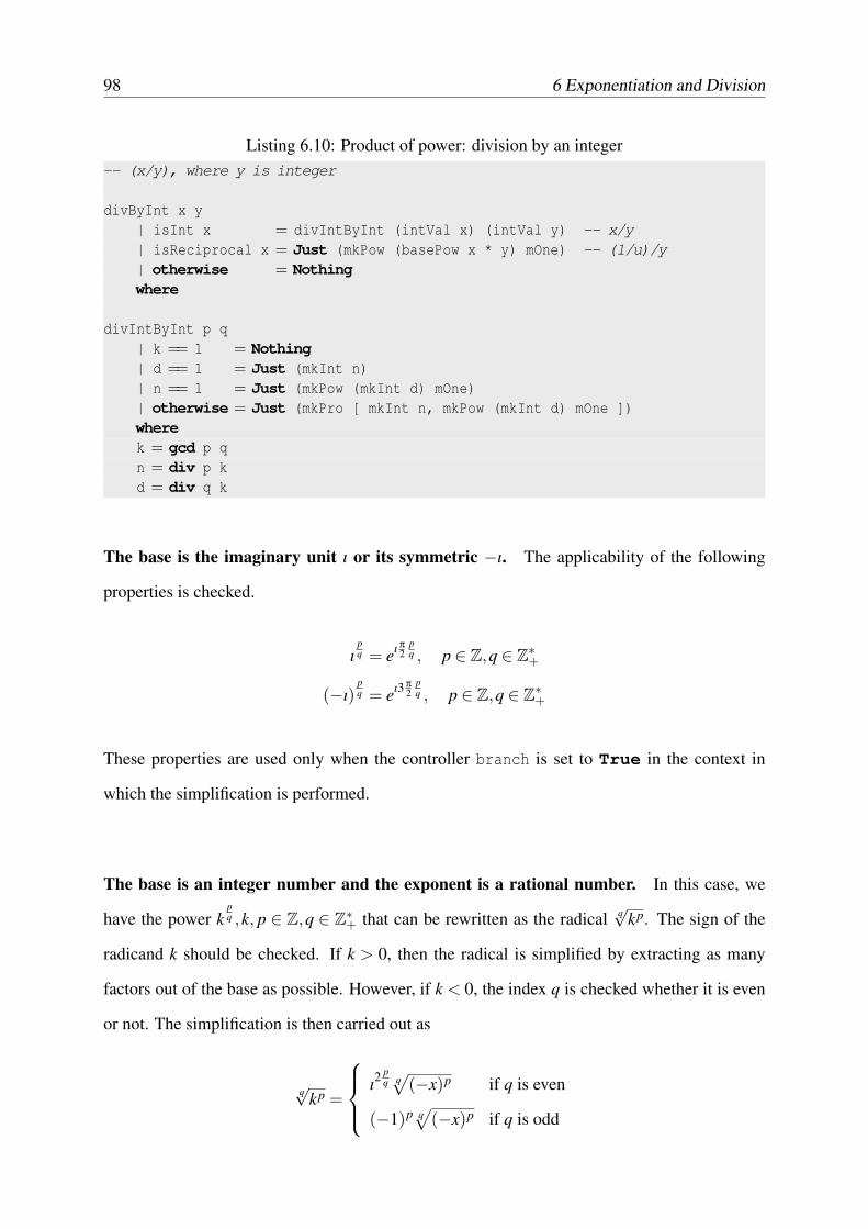
Listing 6.10: Product of power: division by an integer-- (x/y), where y is integer
divByInt x y| isInt x = divIntByInt (intVal x) (intVal y) -- x/y| isReciprocal x = Just (mkPow (basePow x * y) mOne) -- (1/u)/y| otherwise = Nothingwhere
divIntByInt p q| k == 1 = Nothing| d == 1 = Just (mkInt n)| n == 1 = Just (mkPow (mkInt d) mOne)| otherwise = Just (mkPro [ mkInt n, mkPow (mkInt d) mOne ])wherek = gcd p qn = div p kd = div q k
The base is the imaginary unit ı or its symmetric −ı. The applicability of the following
properties is checked.
ıpq = eı π
2pq , p ∈ Z,q ∈ Z∗+
(−ı)pq = eı3 π
2pq , p ∈ Z,q ∈ Z∗+
These properties are used only when the controller branch is set to True in the context in
which the simplification is performed.
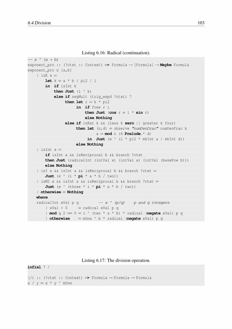
The base is an integer number and the exponent is a rational number. In this case, we
have the power kpq ,k, p ∈ Z,q ∈ Z∗+ that can be rewritten as the radical q
√kp. The sign of the
radicand k should be checked. If k > 0, then the radical is simplified by extracting as many
factors out of the base as possible. However, if k < 0, the index q is checked whether it is even
or not. The simplification is then carried out as
q√
kp =
ı2pq q√
(−x)p if q is even
(−1)p q√
(−x)p if q is odd
6.4 Division 99
These properties are implemented in the code shown on listings 6.15 and 6.16, and must be
used only when the controller branch is set to True in the context in which the simplification
is performed.
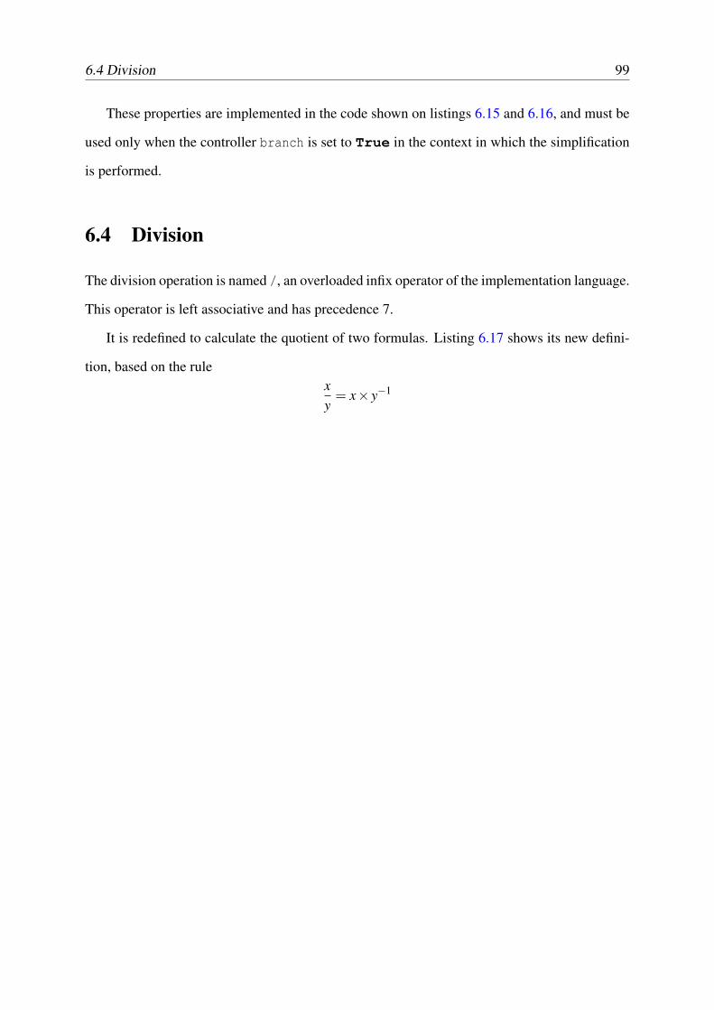
6.4 Division
The division operation is named /, an overloaded infix operator of the implementation language.
This operator is left associative and has precedence 7.
It is redefined to calculate the quotient of two formulas. Listing 6.17 shows its new defini-
tion, based on the rulexy
= x× y−1
100 6 Exponentiation and Division
Listing 6.11: Product of power: division by a sum-- x / (y1 + y2 + ... + yn)---- a) (x1 * x2 * ... * xm) / y = (x1/y) * (x2/y) * ... * (xm/y)-- b) (1/u) / (y1 + y2 + .. + yn) = 1 / (u*y1 + u*y2 + ... + u*yn)-- b) x / (y1 + y2 + ... + yn) = 1 / (y1/x + y2/x + ... + yn/x)
divBySum x ys| isPro x = Just (distribFactors (appArgs x) [] [])| isDen x = distribDen (x ^ mOne)| num_den ?ctxt > 0 &&
num_den’ x = Just (mkPow (distrib’ (x ^ mOne) ys) mOne)| otherwise = NothingwheredistribFactors [] l1 l2 =
distribFactors (u:us) l1 l2| isDen u = if den_den ?ctxt > 0 && den_den’ v
then distribFactors us (v:l1) l2else distribFactors us l1 (u:l2)
| num_den ?ctxt > 0 &&num_den’ u = distribFactors us (v:l1) l2
| otherwise = distribFactors us l1 (u:l2)wherev = u ^ mOne
distribDen u| den_den ?ctxt > 0 &&
den_den’ u = Just (mkPow (distrib’ u ys) mOne)| otherwise = Nothing
distrib’ x ys = distrib x yswith ?ctxt = ?ctxt { num_num = den_den ?ctxt
, den_num = num_den ?ctxt}
-- distrib x ys-- multiply x and each element of ys and then add the resultsdistrib x ys =
mkSum (foldr (\y zs→ mergeSum (x * y) zs) [] ys)
Listing 6.12: Product of power: overloaded functionsinstance ProC FnArith where
proT Pow ctxt xs y = pro_pow xs y with ?ctxt = ctxt. . .
6.4 Division 101
Listing 6.13: Prower of a product.-- (x * y) ^ z = x^z * y^z-- when exp_bas > 0, distributes the exponent over a productbase_pro :: (?ctxt :: Context) => [Formula]→ Formula→ Maybe Formulabase_pro [x,y] z
| exp_bas ?ctxt > 0 && exp_bas’ z = Just (x^z * y^z)| otherwise = Nothing
instance BaseC FnArith wherebaseT Pro ctxt xs y = base_pro xs y with ?ctxt = ctxt. . .
Listing 6.14: Power of a power.-- (x ^ y) ^ zbase_pow :: (?ctxt :: Context) => [Formula]→ Formula→ Maybe Formulabase_pow [x,y] z
| isInt z || branch ?ctxt = Just (x ^ (y * z))| otherwise = Nothing
instance BaseC FnArith wherebaseT Pow ctxt xs y = base_pow xs y with ?ctxt = ctxt. . .
| p Prelude.* p > n = True| mod n p == 0 = False| otherwise = verify ps
6.4 Division 103
Listing 6.16: Radical (continuation).-- x ^ (a * b)exponent_pro :: (?ctxt :: Context) => Formula→ [Formula]→ Maybe Formulaexponent_pro x [a,b]
| isE x =let k = a * b / pi2 / iin if isInt k
then Just (i ^ k)else if negMult (trig_expd ?ctxt) 7
then let r = k * pi2in if free r i
then Just (cos r + i * sin r)else Nothing
else if isRat k && (less k zero || greater k four)then let (n,d) = observe "numDenDrac" numDenFrac k
a = mod n (4 Prelude.* d)in Just (e ^ (i * pi2 * mkInt a / mkInt d))
else Nothing| isInt x =
if isInt a && isReciprocal b && branch ?ctxtthen Just (radicalInt (intVal x) (intVal a) (intVal (basePow b)))else Nothing
| isI x && isInt a && isReciprocal b && branch ?ctxt =Just (e ^ (i * pi * a * b / two))
| isMI x && isInt a && isReciprocal b && branch ?ctxt =Just (e ^ (three * i * pi * a * b / two))
| otherwise = NothingwhereradicalInt xVal p q -- x ^ (p/q) p and q integers
| xVal > 0 = radical xVal p q| mod q 2 == 0 = i ^ (two * a * b) * radical (negate xVal) p q| otherwise = mOne ^ b * radical (negate xVal) p q
Listing 6.17: The division operation.infixl 7 /
(/) :: (?ctxt :: Context) => Formula→ Formula→ Formulax / y = x * y ^ mOne
Chapter 7System Organization
In this chapter the author presents the module organization of the library. He also explains how
to extend the system with new modules. Another discussed topic is performance comparison of
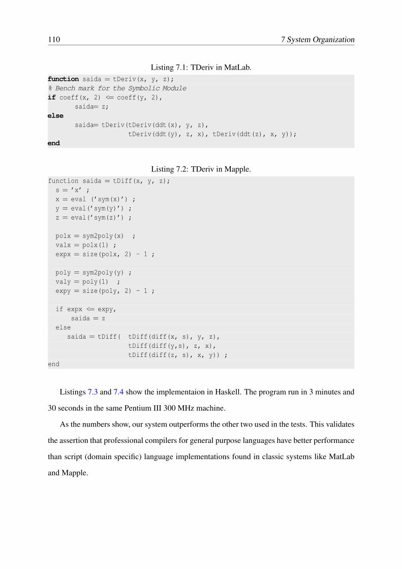
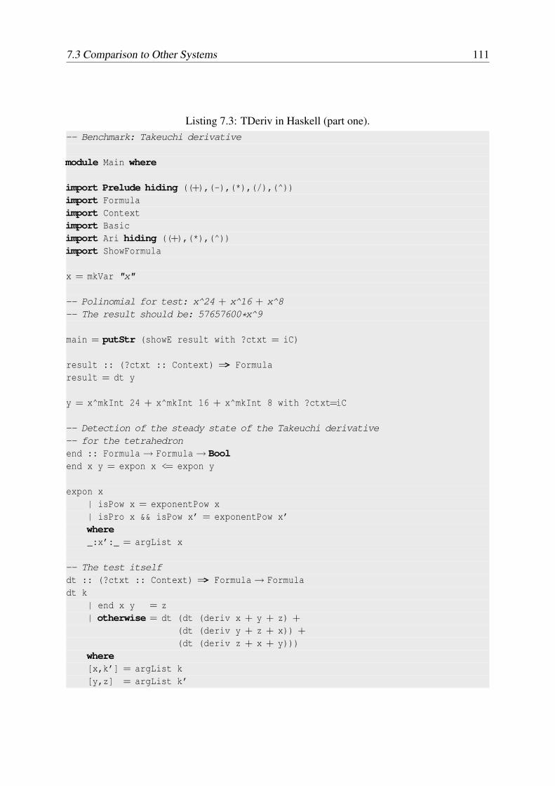
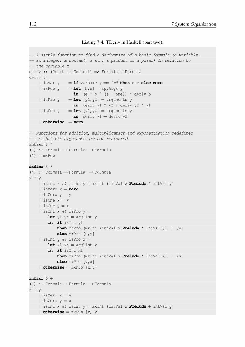
the library against similar systems implemented with different approaches.
7.1 Module Organization
The library is organized as collection of modules, described in the following.
SubType Introduces the subtype relationship among two types, based on type classes.
FnClass Introduces the class of operators, FnC.
FnArithmetic Defines the data type for the basic arithmetic operators and instantiates it to
the FnC class.
FnLogarithm Defines the data type for the logarithm operator and instantiates it to the FnC
class.
Fn Defines the data type for all operators, the supertype Fn, using union types and the sub-
typing relationship introduced in module SugType.
104
7.1 Module Organization 105
Formula Defines the data type for algebraic formulas (the type Formula), which is based on
the Fn type.
Context Defines the data type of contexts (the type Context) and a suitable context (iC for
initial context) for use a top level simplifications. Depends on the Formula module, as some
controller values are formulas.
Basic Defines basic functions over formulas, needed in almost all other modules. This in-
cludes
• checking for canonical form
• finding the arguments of an application formula
• dealing with rational numbers (reciprocals and fractions, numerators and denominators)
• inequalities (checking if a formula is lesser than another formula)
• checking if a formula has a negative coefficient
• getting the coefficient and the literal parts of a formula
• getting the base and the exponent of a power
CBasic Defines type classes for overloading functions that implement special cases of basic
operations defined in module Basic:
• Class ArgumentsC has the funciton argumentsT which handles special ways of finding
the arguments of an application formula.
• Class NumeratorC has the funciton numeratorT which handles special ways of finding
the numerator of a formula.
• Class DenominatorC has the funciton denominatorT which handles special ways of find-
ing the denominator of a formula.
106 7 System Organization
Eval Defines functions for dynamic evaluation of formulas.
CEval Defines type classes (with the function evalT) to handle special cases of dynamic
evaluation of formulas.
Ari Defines basic arithmetic operations with formulas, including
• finding the minum of two formulas
• finding the absolute value of a formula
• addition of formulas
• multiplication of formulas
• exponentation of formulas
CAri Defines tupe classes for overloading the functions that implement special cases of oper-
ations like additons and multiplication.
• Class SumC has the funciton sumT which handles special cases of addition.
• Class ProC has the funciton proT which handles special cases of multiplication.
• Class BaseC has the funciton baseT which handles special cases of the base of an expo-
nentiation.
• Class ExponentC has the funciton exponentT which handles special cases of the expo-
nent of an exponentiation.
Logarithm Defines functions over logarithm formulas. The function log evalutes the loga-
rithm of a formula.
IBasicLog Defines instances of classes ArgumentsC, numeratorC, and DenominatorC for
sums, products and powers, to deal with special cases of basic functions defined in module
Basic over logarithms.
7.2 Extending the Library 107
IBasic Defines instances of classes ArgumentsC, numeratorC, and DenominatorC for sums,
products and powers, to deal with special cases of basic functions defined in module Basic.
IAriLog Defines instances of classes SumC, ProC, BaseC and ExponentC for logarithms, to
deal with special cases of the basic arithmetic operations (addition, multiplication and exponen-
tiation) when one argument is a logarithm.
IAri Defines all instances of classes SumC, ProC, BaseC and ExponentC, to deal with special
cases of the basic arithmetic operations (addition, multiplication and exponentiation).
IEvalAri Defines instances of the classes defined in CEval to deal with special cases of dy-
namic evaluation of basic arithmetic formulas (sums, products and powers).
IEvalLog Defines instances of the classes defined in CEval to deal with special cases of
dynamic evaluation of arithmetic formulas.
IEval Defines instances of the classes defined in CEval to deal with all special cases of dy-
namic evaluation of formulas.
FormulaParser Defines a parser for formulas, based on monadic parser combinators.
ShowFormula Defines a print printer for formulas.
Main Defines an interactive evaluator of algebra formulas, with a read–eval–print loop.
7.2 Extending the Library
In order to extend the library with new kinds of formulas and/or new operations over formulas,
the user should provide the new data type and/or function definition, toghether with instances
of any relevant classes that deal with special cases.
108 7 System Organization
Consider the extension of the library with derivatives. The following modules should be
added to system to complete the support for the derivative operation:
• FnDer with a data type declaration for the operator used with derivative formulas.
• Der with the definition of the function der for finding derivatives of formulas.
• CDer with the definition of a type classe CDer that overloads a function derT to deal with
special rules for finding the derivates. For example, the derivative of a sum is the sum of
the derivatives, is a special rule.
• IDerAri with instances of class CDer that defines the overloaded function derT for the
basic arithmetic formulas (sums, products and powers).
• IDerLog with instances of class CDer that defines the overloaded function derT for log-
arithm formulas.
• IDer with alls instances of class CDer
Some modules should be added or modified to implement special rules concerning derivatives
for the operations already defined, like addition, multiplication and exponentiation. For exam-
ple, the sum of a derivative is the derivative of the summands.
• IAriDer with instance definitions of the classes defined in module CAri, specifying the
rules for adding, multiplying and exponentiating derivatives.
• IAri should be modified to include the new instances from IAriDer|.
• Similarly, if the other operations have special rules for operating on derivatives, the cor-
responding classes should be instantiated accordingly.
As can be noted, the extension of the library with a new kind of formula is reflected in a
set of new modules, and the modification of few ones. If the actual Haskell implementations
had good support for mutually recursive modules, these modules could be reduced in number,
making the system organization simpler.
7.3 Comparison to Other Systems 109
7.3 Comparison to Other Systems
Most successfull Computer Algebra systems available today have been crafted by a large group
of dedicated programmers. This means that special attention could be devoted to the issues
of performance of the system, finding most bottlenecks as well as ways of solving them. For
instance, the Mathematica system is capable to analyse the code to be processed, seeking for
common patterns of simplifications and achieve good performance by handling them as very
special cases. If a problem does not fall in such cases, its performance might not be so good.
As a consequence, the implementation of those systems has a very high level of complexity.
This, added to the low level of abstraction of their implementation language (mostly are written
in C or Lisp), greatly difficults their implementation and mantainability.
Also, in most of those computer algebra systems, the implementation language and the
language used for develepment in the system are distinct languages. The last one is usually an
interpreted language and, as a consequence, programs developed in these systems have lower
performance than programs written in compiled languages.
The computer algebra system developed in this work is implemented in and uses as the
language for development, the same language — Haskell. The choice of this language as the
implementation language contributes for easing the system development and maintanability, due
to the higher level of abstraction found in modern functional languages. It is also expected that
program development and maintenance in our system be easier than in other existing algebraic
system, for the same reason.
To compare the performance of our system to some other successfull Computer Algebra sys-
tems, we run the classical benchmark TDeriv (the Takeuchi derivative). Listing1 7.1 shows its
implementaion in MatLab. It was run using the derivative implementation provided by MatLab.
This program took about 14 minutes to run in a Pentium III 300MHz computer.
Listing 7.2 shows its implementaion in Mapple. When run with the call
tDiff(’x^24’, ’x^16’, ’x^8’), this program took about 14 minutes to complete, in the
same Pentium III 300 MHz computer.
1The MatLab and Mapple tests were conducted with the help of Antônio Cláudio Pascoareli Veiga, from theElectrical Engeneering Faculty at the Universidade Federal de Uberlândia.
110 7 System Organization
Listing 7.1: TDeriv in MatLab.function saida = tDeriv(x, y, z);% Bench mark for the Symbolic Moduleif coeff(x, 2) <= coeff(y, 2),
saida= z;else
saida= tDeriv(tDeriv(ddt(x), y, z),tDeriv(ddt(y), z, x), tDeriv(ddt(z), x, y));
end
Listing 7.2: TDeriv in Mapple.function saida = tDiff(x, y, z);
-- Polinomial for test: x 24 + x 16 + x 8-- The result should be: 57657600*x 9
main = putStr (showE result with ?ctxt = iC)
result :: (?ctxt :: Context) => Formularesult = dt y
y = x^mkInt 24 + x^mkInt 16 + x^mkInt 8 with ?ctxt=iC
-- Detection of the steady state of the Takeuchi derivative-- for the tetrahedronend :: Formula→ Formula→ Boolend x y = expon x <= expon y
expon x| isPow x = exponentPow x| isPro x && isPow x’ = exponentPow x’where_:x’:_ = argList x
-- The test itselfdt :: (?ctxt :: Context) => Formula→ Formuladt k
| end x y = z| otherwise = dt (dt (deriv x + y + z) +
(dt (deriv y + z + x)) +(dt (deriv z + x + y)))
where[x,k’] = argList k[y,z] = argList k’
112 7 System Organization
Listing 7.4: TDeriv in Haskell (part two).
-- A simple function to find a derivative of a basic formula (a variable,-- an integer, a contant, a sum, a product or a power) in relation to-- the variable xderiv :: (?ctxt :: Context) => Formula→ Formuladeriv y
| isVar y = if varName y == "x" then one else zero| isPow y = let [b,e] = appArgs y
in (e * b ^ (e - one)) * deriv b| isPro y = let [y1,y2] = arguments y
in deriv y1 * y2 + deriv y2 * y1| isSum y = let [y1,y2] = arguments y
in deriv y1 + deriv y2| otherwise = zero
-- Functions for addition, multiplication and exponentiation redefined-- so that the arguments are not reorderedinfixr 8 ^(^) :: Formula→ Formula → Formula(^) = mkPow
infixr 8 *(*) :: Formula→ Formula → Formulax * y
| isInt x && isInt y = mkInt (intVal x Prelude.* intVal y)| isZero x = zero| isZero y = y| isOne x = y| isOne y = x| isInt x && isPro y =
let y1:ys = argList yin if isInt y1
then mkPro (mkInt (intVal x Prelude.* intVal y1) : ys)else mkPro [x,y]
| isInt y && isPro x =let x1:xs = argList xin if isInt x1
then mkPro (mkInt (intVal y Prelude.* intVal x1) : xs)else mkPro [y,x]
| otherwise = mkPro [x,y]
infixr 6 +(+) :: Formula→ Formula → Formulax + y
| isZero x = y| isZero y = x| isInt x && isInt y = mkInt (intVal x Prelude.+ intVal y)| otherwise = mkSum [x, y]
Chapter 8Conclusions
8.1 Conclusions
We feel our objective of constructing a library of functions for high level manipulation of al-
gebraic formulas in a pure functional language has been achieved. Although these days the
scenario for programming languages is still dominated by the imperative languages, there is
nothing that forbides the use of declarative languages for solving real world problems. In par-
ticular, the functional languages are ready for use by the software industry and our system is
just an example of how that can be done. One can benefit from the higher level of these lan-
guages for the description of data and algorithms without making sacrifices to the efficiency of
the resulting system, as there are good implementations of functional languages. For instance,
the implementation of the Haskell language, the language we have been using in this project, is
very good, sometimes better than implementations of conventional languages like C.
One could argue the point that functional languages lack good libraries for general use.
This is not always the case. Good libraries are being constantly developed by the functional
programming community. We have just added our contribution to the community of functional
programmers with a new library of Computer Algebra that can be used with no restrictions.
We worked out algorithms for manipulation of algebraic formulas based on earlier works
with non pure functional languages like Scheme and Lisp. Again, it was a new contribution
since there was no such system that was not based on any kind of change of state. Even the
113
114 8 Conclusions
ones programmed in the (non pure) functional languages are not declarative since they rely on
some sort of state changing.
We developed a library of functions for algebraic manipulation in Haskell, a modern func-
tional language, leading to an embedded domain specif language for Computer Algebra. The
library provides types for the representation of algebraic formulas, as well as basic functions
(core) for algebraic manipulation. The library is also easily extensible. Our approach was the
design and language adequacy analisys.
One difficulty we found was how to express some characteristics of the original algorithms
without relying on state changing. The solution was to use implicit parameter passing, which
provides a kind of dynamic scoped parameters. This way the context (set of controllers telling
in which ways the formulas should be transformed) is not explicitly passed in function appli-
cations, keeping the intended arity of operators like +. If the transformation of the algebraic
formula demanded an auxiliary transformation on (possibly part of) the formula with a differ-
ent set of controllers, the appropriate function is called with the usual explicitly parameters
(the formulas to be manipulated) and a new set of controllers, implicitly passed. The prior set
of controllers does not have to be changed. When returning from the auxiliary function, the
original controllers are still intact. There is really no change in state during computation. If
the user needs or wants to prove correctness of the algorithms she/he implemented, referential
transparency allows the substitution of equals for equals, making the reasoning much simpler
than in the absence of referential transparency. Undoubtedly this is one of the most appealing
advantages of functional programming.
Other major difficult that we dealt with was how to achieve a modular, easily extensible
system. It should be easy to add new kind for algebraic formulas and/or operations to the
system without breaking any working programs. Two solutions were investigated. The one
adopted is based on extensible union data types and is based on a mechanism that permits the
extension of a data type with new value constructors (a kind of restricted subtyping). Function
extensions is based on overloading with type classes. Another solution is to use existentially
quantified type variables and type classes to build an object oriented approach. Each kind of
formula has its own data type, which is a subtype of a more general type for all formulas, and a
8.2 Future Work 115
set of specialized functions.
All solutions to these difficulties are based on concepts not incorparated into the Haskell
standard yet. The extended Haskell has shown adequate to the implementation of the library,
offering a high level of abstraction.
It is interesting to note that the author’s proposal is an embeded system for Computer Al-
gebra aplications development. Building it on top of a well-stablished and high-level language
make all the facilities of the hosting language available for the programmer, adding new fea-
tures to it. Few implementations of Computer Algebra systems take this approach. Most of
them have their own programming language.
The reasearch has started with a prototype of the library in Scheme1. It helped to better
understand the algorithms. Then entered Haskell to provide a modern functional language with
static type checking. Finally Clean has been targeted, as a more efficient functional language
with all the properties of modern functional languages. This work describes just the Haskell
part of the research.
8.2 Future Work
Our system uses a context that carries information on how to produce a unique simplification of
an expression. This may be restrictive and a more general solution would compute all the pos-
sible simplications, eliminating the need of the context. It may be desirable that the algorithms
be revised or even redesigned to be free of the need for context. This would be a major work.
A major ambitious project is to extend this system to the context of Pure Algebra and treat
things like groups and rings. In this direction there is already DoCon, a work being developed
by Sergey Mechveliani [20]. “DoCon joins the categorial approach to the mathematical compu-
tation expressed via the Haskell type classes, and explicit processing of the domain description
terms.”
1Appendix A has a short review of what have been implemented in Scheme.
Appendix AUsing the System
This system was first implemented in Scheme as a testbed for the algorithms. This implementa-
tion is more complete than what is presented in the thesis body. The following topics have been
covered by it:
• Basic arithmetic
• Basic algebra
• Arrays
• Matrixes
• Absolute value
• Differentiation
• Logarithms
• Trignometry
• Equation solving
• Ordinary differential equation solving
• Integrals
• Limits
116
117
An interactive system where the user is offered a read-eval-print loop where algebraic ex-
pressions can be entered, evaluated, and then the result can be printed. This system is similar to
the one implemented in Haskell and Clean, but it covers more algorithms.
In the sequence there is some examples of interaction with the system.