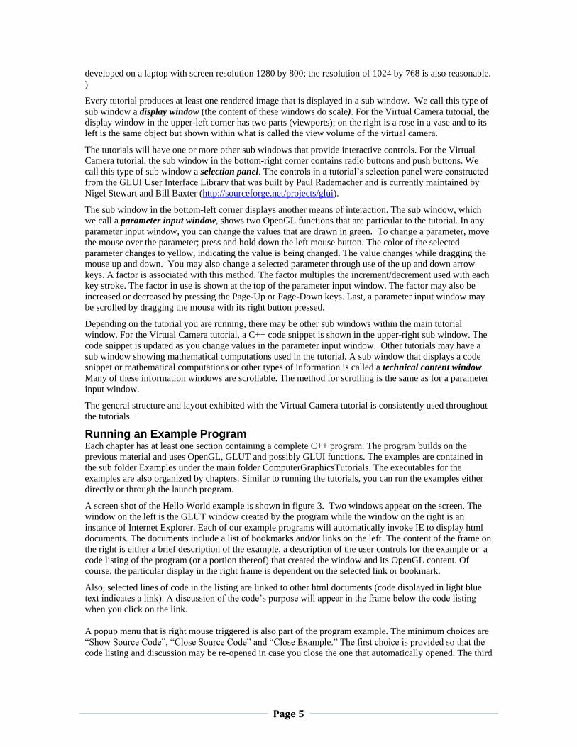
menu choice not only closes the program but it also closes Internet Explorer and its display of the code
listing and ancillary materials.
Figure 3 Hello World Example with Annotated Source Code
Comments on Use of Software As noted in the introduction, the suite of tutorials and examples has evolved over the past 10 years. Also,
the current version has been used for several semesters in an introductory computer graphics course taught
by me. I am sharing herein comments on how it was used in that course.
The course, CS 256 taught at St. Bonaventure University, consists of a “lecture” portion, meeting 2.5 hours
per week, and a closed lab portion, meeting 2 hours per week. The suite is used in both components in
various ways.
It has been said that a picture is worth a thousand words but I add that it is worth even more when it is
interactive. Further, it is understood that students learn best when they are active participants in the process.
Thus, when I used the software in a “lecture”, I asked a student to be the user and “operate” the tutorial
and/or example. But, of course, the student is guided in her exploration with a script that I provide either
verbally or in written form. Appendix B contains samples of three (abbreviated) scripts. The scenarios,
which I call Discovery Activities for lack of a better term, are designed for the students, including the
designated user, to understand through exploration a specific concept and/or specific API function. For
example, activities in the Color Models script are written to discover (understand) saturation in the HSV
model and the effect occurring in the RGB model when changes are made to the color’s saturation. In turn,
it is hoped that the student develops an understanding of the relationship between the two models. The
scenarios easily extend during a “lecture” beyond the ones I initially provide since all students are
encouraged to suggest other activities.
Page 7
Assignments in the closed labs may take one of two forms. One form is a script of Discovery Activities and
the student is required to submit her recorded observations. Another form is the somewhat traditional “write
a program that ….” Lab assignments may also be a combination of the two. For example, the first closed
lab in CS 256 pertains to the Hello World program. The first sample script in Appendix B suggests part of
the assignment; the other part requires the student to submit a modified Hello World program. Obviously,
the first lab serves as an “ice breaker” and, in turn, is not overly demanding. With respect to labs that
strictly require programming, the assignments are either extensions of the examples or are programs
requiring development “from the get-go” and are based on concepts presented in the tutorials. The latter
type of lab assignment indicates why I have chosen to have example software and tutorials in the suite. The
program examples are just that with the entire source code visible to the student. On the other hand, a
tutorial focuses on a concept with its source code not being pertinent to the learning objective. I may give,
for example, a lab assignment that requires the student to incorporate the viewing transformation within her
program. Or I may ask that a program be written that produces a shadow on a plane that is not one of the
coordinate planes. For this latter example, the Projection Shadow tutorial gives the student the necessary
information on computing the projection transformation.
I hope that you find the suite of tutorials and examples useful in these and other ways when teaching an
introductory computer graphics course.
Dalton R. Hunkins
References Hunkins, Dalton and Levine, David, “Additional Rich Resources for Computer Graphics Educators”,
Computers and Graphics, 2002, Vol. 26, No. 4, pp. 609-614.
Hunkins, Dalton and Levine, David, “Rich Resources for Computer Graphics Education”, SIGGRAPH
2001 Educators Forum, Los Angeles, June 2001, pp. 45-48.
Page 8
Appendix A: Annotated Table of Contents
Chapter 0: Our First World Example: Hello World This is our first example of a graphics program. It shows how to create a window using the GLUT library
and create a very simple image in that window using OpenGL functions.
Chapter 1: 2D Projection and Viewports Tutorial: Orthographic Projections With this tutorial you will be learning about projection windows and viewports.
Example: Viewports We use the geometry of our Hello World example and produce two instances of it. The instances are
accomplished through the use of two view ports.
Chapter 2: Color, Geometry and Shading Tutorial: Color Models The tutorial is designed to help you develop intuition about the two color models RGB and HSV. The
models are depicted, respectively, with a cube and a hexcone. By giving input values for either model, you
can develop intuition for color mixing within each model along with an understanding of the relationship
between the two models.
Tutorial: Geometry You see in this tutorial how to construct basic geometries in OpenGL. The geometries include lines,
triangles, quadrilaterials and polygons.
Tutorial: Smooth Shading The focus in this tutorial is the computations used to determine the color of "interior"
points of a triangle using smooth shading (also called Gouraud shading). You are presented with a triangle
having vertex colors red, green, and blue. You select a point of interest within the triangle and the
interpolation computations for that point are then displayed. You may focus your attention on either the
final computation for the selected point or upon one of the intermediary computations.
Example: Cascading Squares The example illustrates the creation of a geometric pattern. The pattern is a sequence of nested squares with
the squares' color saturation decreasing as the squares become smaller. The pattern is created through
recursive function calls.
Example: Circle Disk Line strip (and loop) is a useful basic geometry for approximating curves. We can vary the smoothness of
the approximating curve by varying the distance between the points in the strip. This is illustrated here with
the construction of a circle. Also, once we have the points for the approximating circle, we can easily
construct a filled circle (i.e, a disk).
Example: GLU Disk The OpenGL utility library glu contains a function for constructing a disk. The example illustrates how to
use the function.
Example: Line Stipple A line is stippled when it is drawn broken and appears as a sequence of dots and dashes. Further, the length
of the visible portions and the length of spaces can be varied as illustrated with this example.
Page 9
Chapter 3: Transformations and Animation Tutorial: 2D Transformations By interacting with this tutorial, you can see how a 2D object is affected with the application of two-
dimensional transformations while also viewing the current transformation matrix that creates the effect.
Example: Many Instances We saw with the example Viewports how we can use different viewports to create several instances of a
geometry. The use of transformations gives another way of creating multiple static instances of a geometry.
The example illustrates this point.
Example: Morphing Using Idle Function Animations are of great interest. We use the basic OpenGl transformations to animate the size, orientation
and/or location of geometries. In this example we use transformations to change the shape of an object. We
also animate the color of the object. In creating the animation, we demonstrate how to the use an idle
function that we register with glut. In particular, our registered idle function calls our display method with a
change between calls to the parameters that control the transformations on the object and the color applied
to the object.
Example: Morphing Using Timer Function The animation is the same as the one demonstrated in the previous example. Except in this example we
create the animation through the use of a timer function that we register with glut. The advantage in using a
timer function versus an idle function allows us to make the speed of the animation platform independent
by setting the frame rate of the animation.
Chapter 4: Menu, Keyboard and Mouse Interaction Example: User Interaction through GLUT We see with this example how to create interactive methods using glut. These include the use of the mouse
for picking an object within the world and dragging the object. We also see how to create a popup menu
and define keyboard handlers.
Chapter 5: Texture Mappings Tutorial: Texture Coordinates The tutorial guides you through understanding what is needed to accomplish the application of a texture
(bitmap) to a geometry in two dimensions.
Tutorial: Texture Transformations The tutorial follows the one on texture coordinates. It is suggested that you do the Texture Coordinate
tutorial before doing this one.
Example: Image Map The example has two image maps where either of the two can be applied to different geometries. The
geometries consist of squares, a hexagon and an octagon. The application of a map to a square is straight
forward. But the calculations of the texture coordinates corresponding to the vertices of the hexagon and
the octagon are a bit more complicated.
Chapter 6: A Little Game Programming Example: Game with Stationary Targets This example illustrates a simple third person shooting game. The game consists of a rotating tank that fires
projectiles and five stationary targets. Discussion is given here on how we decide when a projectile will hit
a target. This game provides one of the simplest cases of collision detection -- a moving object along a
straight line and a stationary target.
Page 10
Example: Game with Moving Target This is the first in a series of two in which a moving target is added to our shooting game with stationary
targets. Our method of collision detection used with stationary targets can be used with the moving target if
the moving target stops when the projectile is fired. Guess what happens in this version of the game.
Example: Shooting Game (final version) Collision detection in this version of the game is with both objects moving. The calculations are still
relatively simple since the two motion paths are straight lines. Note that in a real situation, collision
detection requires knowing not only the motion paths but also the velocities of each object. With this
information we compute whether the two objects will arrive at the collision point at the same time. Time in
our synthetic world is measured by frames and, in turn, our question is will the two moving objects arrive at
the collision point in the same frame.
Chapter 7: Virtual Camera Tutorial: Virtual Camera A key concept in computer graphics is to model a world and then "take a picture" of the world through a
(virtual) camera. We first establish the camera in OpenGL by setting its location, the direction it points and
its orientation, also called its roll. Next, we establish the type of projection to be applied, either
orthographic or perspective. The tutorial, in turn, is designed to help you understand this fundamental
concept of viewing and how it is accomplished in OpenGL.
Tutorial: Camera Motion The standard camera movements include orbit, pan, truck and dolly. By interacting with this tutorial, you
can see the effect of each of these camera moves on the projected image.
Tutorial: The Viewing Transformation Matrix The tutorial shows the computations used by OpenGL in determining the viewing transformation matrix.
This matrix is created by OpenGL when a call is made to gluLookAt.
Chapter 8: Lighting Tutorial: Ambient Reflection The tutorial focuses on the determination of color using the Phong Illumination Model. In particular, you
control the color of an ambient light as it illuminates four swatches of material (cyan, yellow, magenta, and
gray). The color computations for any one of the materials you choose are shown in one sub window while
the visual effect of the computation is displayed in another sub window.
Tutorial: Diffuse Reflection The tutorial helps you understand the lighting effects of omni and directional lights on a simple scene
consisting of two planes meeting at a corner. Further, the effect involves diffuse reflectivity and is
determined by the orientation of surface normals to the lights. You can change the lighting effects by
manipulating the normals.
Tutorial: Specular Reflection The tutorial demonstrates specular reflectivity as created by a spot light illuminating a sphere. Also, you
can change the cutoff angle and the exponent of the light and see the effect of the changes by viewing the
illumination of the light on the background.
Example: Lights The example illustrates the use of four lights, ambient, omni, directional and spot, to illuminate our world.
Page 11
Chapter 9: Miscellaneous Tutorial: Bezier Spline A spline consists of curves placed end-to-end. We consider in this tutorial Bezier curves that are part of
OpenGL. We also show how the splines obtained from these curves can be used as motion paths, to obtain
a surface through extrusion and to obtain a surface of revolution.
Tutorial: A Projected Shadow The tutorial demonstrates how a shadow can be cast onto a plane by computing a projection matrix and
applying it to the 3D geometry. We also set the drawing color to one appropriate for the shadow and apply
it to the projected geometry.
Tutorial: Ray Traced Shadow The tutorial applies the method used in a Ray Trace render for creating shadows. The demonstration shows
the calculations for "casting" a shadow onto a plane by one of three types of objects -- a sphere, a hollow
cylinder (one without end caps) and a solid cylinder (one with caps).
Example: Two-Sided Material OpenGL provides the means to assign different materials to two sides, the outside and the inside, of the
geometry. In this example, you can cut away the geometry, which is of course hollow, and see both the
inside and outside of the geometry. You create the cut-away by moving the near plane of the virtual
camera.
Example: Inside a Sphere Generally the background of our synthetic world is static. If we want the background to change as we
animate the camera, then we can place the background on the inside of a sphere and have the sphere
surround the geometry and the camera, as done in this example.
Example: Transparency We have seen with the tutorial Texture Transformations how to make a portion of an image map
"invisible." We do this by setting the alpha component of the texel's color to zero and apply alpha bending.
This can also be accomplished when using a base color or material color for an object. The example also
illustrates how to use the GLUI library in creating an interface for user input.
Example: Texture Methods We have seen in chapter 5 two of the OpenGL methods, namely GL_REPLACE and GL_DECAL, for
applying a image map to a geometry. A third method GL_MODULATE is demonstrated in the example.
You can also compare the effect created with this method in contrast to GL_DECAL. Also, part of the user
interface is created with the GLUI library. Note that this example is located here versus chapter 5 since the
effect of modulate is best appreciated when lighting is present.
Example: Model Viewer The tutorial Camera Animation is a model viewer but with only one model available. The example
illustrates how to use the GLUI library to open a file browser and select a model to be viewed. Reading the
file and rendering its content is part of the Utils class ObjectModel. You can use this class and any of the
others in Utils when you construct your own programs.
Page 12
Appendix B: Sample Scripts
Modifying Hello World
The source code for Hello World, namely HelloWorld.cpp, resides in the folder ../ExampleSourceCode/Chapter 0/.
Open the program HelloWorld.cpp in your IDE.
As mentioned in the introduction, the IDE used in developing the tutorials is Bloodshed’s Dev-C++
with the Cygwin C++ compiler. However, it does not matter which one you use as long as it is setup to compile programs that make calls to OpenGL and GLUT. The particulars on setting up a specific IDE will not be discussed here since there are many differences between them.
There are a number of changes that we can make to Hello World, each producing a different visual affect. In addition to changing the parameter passed to glLineWidth, try the following.
Discovery Activity: What colors do we obtain?
Using only 0’s and 1’s, vary the parameters passed to glColor3f. Try each of the eight possible combinations (1, 1, 1), (0, 1, 1), etc. Compile and run your modified program. Note that color mixing is covered with the tutorial in chapter 2.
Discovery Activity: Assigning colors to each vertex
Place a copy of the call to glColor3f before each of the four calls to glVertex2d. Assign different color values to the four calls to glColor3f. Compile and run the modified program and observe how these changes affect the rendered image.
Discovery Activity: What happens if we use a coordinate larger than 1.0 or smaller than 0.0?
Change one or more of the vertices so that at least one of its coordinates (x or y or both) is bigger than 1.0 and/or less than 0.0. How does this change the rendered image? Keep in mind the boundaries of the projection window are defined in the call to gluOrtho2D,.
Discovery Activity: Does the call to glFlush really matter?
Comment out the call to glFlush and compile and run the modified program. Is the call to glFlush necessary? Why?
Page 13
Exploring with the Orthographic Projection Tutorial
Run the Orthographic Projection tutorial that is in chapter 1.
Discovery Activity: Setting the Projection Window
We are going to change the boundaries of the projection window so as to select certain portions of the world for rendering. You accomplish this by changing the boundary parameters appearing in the parameter input window on the bottom-left side. Also, the technical content window appearing on the bottom-right side shows the coordinates of the rectangles.
Set the boundaries of the projection window so that only the red rectangle appears in the actual display window with a black border around it.
Obviously you can carry out this activity by simply changing the boundaries while watching the projection window in the road-map window. But keep in mind that this visual is not available when writing your graphics programs; you will be setting the projection window boundaries based on the coordinates of the geometries within your world. Uncheck the box “Show Projection Window” in the selection panel and carry out the next activity.
With the projection window not visible in the road-map window, set the boundaries of the projection window so that only the red and green rectangles appear in the actual display window with a black border around them.
Did you pick the left boundary smaller than -30 (e.g. -31) and the right boundary bigger than 15 (e.g., 16)? Also did you pick the bottom boundary smaller than -40 (e.g., -41) and the top boundary larger than 15 (e.g., 16)? How can we determine these boundary values from the coordinates of the rectangles?
Looking at the coordinates of the rectangles, can you pick the boundaries of the projection window so that the red, green, blue and yellow rectangles are displayed AND no portion of any other rectangle? Why or why not?
Discovery Activity: Setting the Viewport
Observe that the shape of the cyan rectangle is tall and skinny. Let us see how it is displayed when we make it the only object in the projection window.
With the projection window not visible in the road-map window, set the boundaries of the projection window so that only the cyan rectangle appears in the actual display window with a black border around them.
Depending on the amount of border you leave around the rectangle, the rectangle appears almost as a square when rendered to the display window. Remember that the projection window is mapped (rendered) to the entire viewport. So, if the projection window is tall and skinny and the viewport is square, the contents of the projection window will be stretched and distorted. In order to avoid the distortion, we have to set the dimensions of the viewport so that it has the same aspect ratio as the projection window. We define the aspect ratio of a rectangle as the quotient
width of rectangle / height of rectangle
A call to glViewport is shown in the parameter input window. The changeable values displayed here are percentages of the width and height; as mentioned, this is a convenient way of setting the boundaries of the viewport.
Keeping the projection window set so as to contain only the cyan rectangle and leaving the left and bottom boundaries of the viewport at 0, change the dimensions of the viewport so that its aspect ratio is the same as that of the projection window.
Did you observe that since the desired aspect ratio is less than one, we need only decrease the width of the viewport to achieve that ratio? Also, the rendered image appears on the left side of the actual display window.
Page 14
Keeping the aspect ratio you set, change a boundary (or boundaries) of the viewport so that the displayed image of the cyan rectangle appears centered in the actual display window.
Did you change only the left boundary of the viewport to achieve the desired affect?
We close this section with the following suggestion.
Use a piece of graph paper when designing your virtual world and label the coordinates of all the vertices within your world.
Page 15
Exploring with the Color Models Tutorial
Run the Color Models tutorial that is in chapter 2.
Discovery Activity: What is Hue?
Click on the second value of rgb[], which sets the green value in RGB, and drag the mouse upward, changing the parameter value from 0.0 to 1.0. Observe the changes in the color models with changes to this green value.
Observe how the color changes from red to yellow. Also note how the ball moves in the RGB model and the HSV model. You will also see the value for hue changing from 0.0 to 60.0.
Click on the first value in rgb[], which sets the red value, and drag the mouse downward, changing the value from 1.0 to 0.0.
Observe that the ball moves along the edge of the hexcone base and the edge of the cube that connects yellow to green. Also the hue parameter changes value from 60.0 to 120.0.
Use the mouse to change the blue value from 0.0 to 1.0
What color changes take place and how does the value for hue change? You should observe that the color changes from green to cyan and hue changes from 120.0 to 180.0.
Use the mouse to change the green value back to 0.0.
After which, increase the red value to 1.0.
Last, decrease the blue value to 0.0, taking us back to full red.
Note that the ball continues to move along the base of the hexcone in a counterclockwise fashion and the value of hue continues to increase through the values 240, 300 and then back to 0. Also observe how the ball moves in the RGB cube, namely along the edges connecting the primary (red, green and blue) and secondary (yellow, cyan and magenta) colors.
Hue is generally what people refer to when talking about color; it is similar to the colors of the rainbow. Hue in the HSV model is represented by the angle in degrees measured counterclockwise around the center of the base of the hexcone. The range of hues is [0, 360) with red = 0, yellow = 60, green = 120, etc. Let us confirm our observations with the following.
Click on the hue value and drag the mouse upward, changing the value from 0.0 through the values 60.0, 120.0, 180.0, 240.0, 300.0 and then back to 0.0.
Yes, the ball moves along the edges of the base of the hexcone in the HSV model and along the edges of the RGB cube connecting the primary and secondary colors.
Page 16
We have been observing color thus far at its full purity and brightness. The values in the HSV model that control these properties are respectfully saturation and value. The two can both be set with numbers in the range [0.0, 1.0].
Discovery Activity: What is Saturation?
Click on the saturation component for the array hsv[] and drag the mouse up and down, changing it between the numbers 0.0 to 1.0.
Observe that when hue = 0, the color goes between red and white through variations of pink. Thus, saturation measures the purity of the color where maximum purity is when saturation = 1.0. When saturation = 0.0 (and value = 1.0), the color is white. Observe also the changes that take place in the RGB model. As the color red decreases in purity, the green and blue components increase equally to 1.0 resulting in the color white and the ball at the vertex (1.0, 1.0, 1.0). Similar changes occur for any of the primary and secondary colors.
Set red and green to 1.0 and blue to 0.0 in the RGB model and, in turn, make the color yellow. Now change saturation from 1.0 to 0.0.
Observe how the color changes to a pale shade of yellow and finally to white. Note also the blue component in the RGB model increases to 1.0.
Discovery Activity: What is Value?
Value, sometimes called brightness, measures the total energy of the color (light) where maximum brightness occurs when value = 1.0. When value is 0.0, the color is black.
Set saturation to 0.0 and value to 1.0 in the HSV model. (Or equivalently, set each of the parameters in the RGB model to 1.0.) Now change the value component of hsv[] from 1.0 to 0.0.
Observe that the ball in each of the models moves along the gray-scale from white to black through shades of gray. In the RGB model, a shade of gray is when the parameters (red, green and blue) are set to the same number.
In summary, saturation in the HSV model measures the relative distance of a point to its axis (gray scale) while value measures the relative height of the point from the apex of the hexcone. We can also think of saturation and value in the RGB model, although it is not as intuitive as in the HSV model. Since saturation is the purity of the color and corresponds to the difference between the color and white, we can reduce the saturation in the RGB model by moving the color from its current location towards the gray scale. We can also change a color's value in the RGB model by moving along the line going from the color's current position to black. For example, to reduce the value of magenta, which is at the point (1.0, 0.0, 1.0), the point moves along the diagonal line in the red-blue face of the cube from the magenta vertex to the black vertex (0.0, 0.0, 0.0). What happens to saturation when the color reaches black? (Hint: any point on the gray scale has zero saturation). Try it!