Computer Methods in Applied Mechanics and Engineering 199 (2010) 1992–2013
Contents lists available at ScienceDirect
Computer Methods in Applied Mechanics and Engineering
j ourna l homepage: www.e lsev ie r.com/ locate /cma
Asynchronous multi-domain variational integrators for nonlinear hyperelastic solids
Michal Beneš b, Karel Matouš a,⁎,1
a Department of Aerospace and Mechanical Engineering, University of Notre Dame, Notre Dame, IN 46556, USAb Computational Science and Engineering, University of Illinois at Urbana-Champaign, Urbana, IL 61801, USA
⁎ Corresponding author. Department of AerospaceUniversity of Notre Dame, 367 Fitzpatrick Hall of Engin5637, USA. Tel.: +1 574 631 1376.
E-mail address: [email protected] (K. Matouš).URL: http://www.nd.edu/~kmatous (K. Matouš).
We present the asynchronous multi-domain variational time integrators with a dual domain decompositionmethod for the initial hyperbolic boundary-value problem in hyperelasticity. Variational time integrationschemes, based on the principle of minimal action within the Lagrangian framework, are constructed for theequation of motion and implemented into a variational finite element framework, which is systematicallyderived from the three-field de Veubeke-Hu-Washizu variational principle to accommodate theincompressibility constraint present in an analysis of nearly-incompressible materials. For efficient parallelcomputing, we use the dual domain decomposition method with local Lagrange multipliers to ensure thecontinuity of the displacement field at the interface between subdomains. The α-method for timediscretization and the multi-domain spatial decomposition enable us to use different types of integrators(explicit vs. implicit) and different time steps on different parts of a computational domain, and thusefficiently capture the underlying physics with less computational effort. The energy conservation of ournonlinear, midpoint, asynchronous integration scheme is investigated using the Energy method, and bothlocal and the global energy error estimates are derived. We illustrate the performance of proposedvariational multi-domain time integrators by means of three examples. First, the method of manufacturedsolutions is used to examine the consistency of the formulation. In the second example, we investigateenergy conservation and stability. Finally, we apply the method to the motion of a heterogeneous planedomain, where different integrators and time discretization steps are used accordingly with disparatematerial data of individual parts.
and Mechanical Engineering,eering, Notre Dame, IN 46556-
In time-dependent scientific simulations, where different multi-physics solvers are often coupled, the time integrator is animportant component. Typically, the partial differential equations(PDEs) are solved by discretizing the domain spatially using finiteelements or finite volumes, then integrating over time using anumerical ordinary differential equation (ODE) solver. Both thecoupling between domains and the time integration must behandled with care to avoid numerical instability, since the stabilityand accuracy of such coupling are dictated not only by the individuallocal time step limits, but also by the data transfer method acrossthe interface. Moreover, the stability and accuracy requirements fordifferent domains may necessitate different time steps. For example,
a stiff material domain may require small time steps for numericalstability, or a fluid domain may require small time steps to resolveboundary layers accurately, while other material domains maypermit a larger time step.
Another challenge when solving these problems is in the spatialdiscretization, allowing the ability to link domains with non-matchingdiscretizations. Due to their size, these simulations often requireparallel computing, which can be effectively done using domaindecomposition. For elliptic problems, Farhat and Roux [16] proposedthe popular FETI method, which was subsequently extended totransient problems [14]. It enforces continuity between domains byadding an additional constraint with Lagrange multipliers. Park et al.[36] developed a variant using local Lagrange multipliers thatconstrains domains to an intermediate interface rather than directlyto each other. Such an intermediate interface is used in Park et al. [37]and Brezzi and Marini [9] to handle domains with non-matchingmeshes, as illustrated in Fig. 1.
To achieve an efficient, stable, and accurate integrator, severalissues must be addressed. For accurate long time integration, it isdesirable that the integrator conserves energy and preservesmomentum. It is well known, that ODE integrators that discretize
Fig. 1. Domain decomposition with a common interface between domains. Arrowsrepresent the local Lagrange multipliers constraining each domain to the interface.
Fig. 2. Problem description.
1993M. Beneš, K. Matouš / Computer Methods in Applied Mechanics and Engineering 199 (2010) 1992–2013
the differential equation itself, such as Runge-Kutta methods, oftenartificially dissipate energy to achieve numerical stability. To relaxthe time step constraint imposed by stability requirements, mixedmethods or multi-time methods with different time steps for eachdomain were proposed. Belytschko and Mullen [6,7] were the firstto use a mixed explicit–implicit method with a nodal partition,while Hughes and Liu [26,27] introduced a mixed method using anelement partition. Belytschko et al. [8] introduced subcycling forfirst-order problems, and later extended it to non-integer time stepratios [5]. Neal and Belytschko [33] developed subcycling with non-integer ratios for second-order structural problems. Althoughpopular, the stability of second-order subcycling methods has beenelusive. Smolinski and Sleith [40] contrived an explicit subcyclingalgorithm for second-order problems that was proved stable [41],but is less accurate than other algorithms. Daniel [11] showed thatNeal and Belytschko's algorithm is “statistically stable”, but unstablefor certain time steps smaller than the expected stability limit. Morerecently, Combescure and Gravouil [10,21] developed a FETI-liketransient method that enforces continuity of velocities and is provedstable but dissipative for subcycling. Prakash and Hjelmstad [38]improved this method to be stable and non-dissipative for subcycling,but their method is based on binary trees for parallelism and additiveoperator split, rendering it less popular for nonlinear problems andhigh-performance computing.
Another set of integrators proposed in recent years are theVariational Integrators. These are derived by discretizing theLagrangian and applying variational calculus, resulting in methodsthat preserve momentum, do not dissipate energy and are symplectic.As a result they are superior for long time integration. Variationalintegrators have been developed by Veselov [42], Wendlandt andMarsden [43], and Marsden and West [31], among others. Kane et al.[29] showed that the popular Newmark method [34] can also bederived variationally. Lew et al. [30] developed an asynchronousvariational integrator (AVI) and presented its explicit implementa-tion, where each element has its own time step. The parallelimplementation of AVI was presented in Kale and Lew [28].
Time integrators for nonlinear problems and their stabilityhave also generated a high degree of interest. Especially, theenergy-controlling or conserving methods have been investigated[19,20,22]. Time integration schemes that conserve the momentaand dissipate the energy in order to diminish unresolved highfrequency modes, while maintaining good accuracy were delineatedin [3]. Recently, energy-dissipative momentum-conserving timestepping algorithms for finite strain multiplicative plasticity werepresented by Armero [2].
Based on the promising results of the variational integrators andtheir deep mathematical structure, in Section 3 we present a
method for integrating nonlinear problems with domain decompo-sition. In particular, we build on our previous work focused on ODEs[18] and extend it to PDEs for nearly-incompressible materials.Quasi-incompressible material behavior is treated by a three-fieldde Veubeke-Hu-Washizu variational principle [19,32,39]. Note thatmodeling of nearly-incompressible materials is challenging, espe-cially for explicit integrators, since the wave speed →∞ as ν→1/2,and thus Δt→0. We develop an asynchronous integrator that allowseach domain to use its own arbitrary time step and integrator. Weuse a variational approach based on the generalized α-method totake advantage of its favorable properties and enforce the continuityof displacements with a common interface. The constraint is appliedby using local Lagrange multipliers in context of the dual domaindecomposition method. Displacement constraints avoid disconti-nuities between domains in the cases where continuity of velocitiesis only enforced.
In Section 4, we present the energy conservation analysis of ourintegrators for both the synchronous and asynchronous timestepping using the midpoint rule, α=1/2. We follow the approachby Hauret and Le Tallec [22]. By treating the constraints variation-ally, we ensure stability in domain coupling. The synchronousimplicit midpoint version achieves a conditional stability withO(Δt3), while with asynchronous steps it is conditionally stable witha local criterion O((Δtk)2). However, we show that for our commoninterface, the global energy control still holds with O(Δt3). Ourmethod accommodates nonlinear problems very naturally and thehigh degree of parallelism is preserved. Note that rigorous nonlinearstability analysis is not part of this investigation. For linear stabilityanalysis of AVI, we point the interested reader to the work of Fonget al. [17].
We present examples in Section 5 involving the convergencestudy, energy conservation study, and the mixed implicit/explicitintegration test that demonstrates the potential of the method forerror control. Finally, several conclusions are made in Section 6.
The main contributions of the present work are: i) Combinationof the most recent advances in asynchronous multi-domainvariational time integrators with a dual domain decompositionmethod in the context of a mixed three-field de Veubeke-Hu-Washizu variational principle for nearly-incompressible solids. ii)Introduction of a linearly interpolated common interface and thelocal Lagrange multiples in the space/time domain that allow formixed, asynchronous implicit/explicit integration amenable toparallel computation. iii) The energy conservation analysis of themidpoint integrator by the Energy method. iv) Unique examples,based on the Method of Manufactured Solutions, that provide arigorous verification testbeds.
1994 M. Beneš, K. Matouš / Computer Methods in Applied Mechanics and Engineering 199 (2010) 1992–2013
2. Governing equations — continuum problem
Let the open set Ω0⊂R3 be the reference configuration of a given (compressible or nearly-incompressible) body at time t0. Each point X isassociated by a bijective map with its position in that configuration: X→X∈Ω0, as shown in Fig. 2.
In the absence of displacement discontinuities, a unique differentiable deformation map ϕ:Ω0×[0, T]→R3 describing a motion exists, suchthat any displaced position at a current time t∈ [0, T], where [0, T]⊂R+ denotes the time of interest, is determined as x=ϕ(X, t) with thedifference being the displacement field u(X, t)=x−X. The deformation gradient F(X, t) is obtained by taking the gradient of the deformationmap F=∇0ϕ, where ∇0 is the gradient with respect to X, and the Jacobian of the deformation map is given by J(X, t)=det F. We also define theright Cauchy-Green deformation tensor C(X, t)=FTF.
The initial/boundary-value problem of motion reads
ρ0∂2u∂t2
= ∇0 · P + f0 in Ω0 × ð0; TÞ;
u = u0 on ∂Ωu × ð0; TÞ;P · N0 = t0 on ∂ΩP × ð0; TÞ;uðX;0Þ = u0 in Ω0;
∂u∂t ðX;0Þ = u0
in Ω0;
ð1Þ
where ρ0(X, t)= Jρ represents the reference mass density and ρ=ρ(X, t) is the deformed mass density, P=P(X, F(X, t)) is the first Piola-Kirchhoff stress, f0= f0(X, t) denotes the external body force, u0= u0(X, t) is the prescribed displacement on the boundary ∂Ωu, t0= t0(X, t)represents the known surface load on the boundary ∂ΩP andN0 represents the unit normal to ∂ΩP. Here
∂u∂t ðX; tÞ denotes thematerial velocity u(X, t)
and ∂2u∂t2 represents thematerial acceleration ü(X, t), respectively. To render the initial/boundary-value problemwell posed, initial conditions u0
and u.0 are given for both displacement u and velocity u. Note that ∂Ωu0
and ∂ΩP are smooth open disjoint subsets of ∂Ω0 such that
∂Ω0=∂Ωu0∪∂ΩP and the 1-dimensional measure of ∂Ω0−(∂Ωu0
∪∂ΩP) is zero.
2.1. A three-field continuous Lagrangian framework
In this work, we are interested in variational integratorswithin the domain decomposition framework to solve the equation of motion, Eq. (1),in the context of nearly-incompressible material behavior, which requires a special numerical treatment. For clarity and completeness of thepresentation, we start with a continuous variational formulation. The derivation of variational integrators for computing the motion in thediscrete setting will follow analogously. To account properly for a nearly-incompressible material response, we employ a three-field de Veubeke-Hu-Washizu variational principle [19,32,39].
In general, the volume-preserving part of a deformation gradient reads
FðX; tÞ = J−13F; ð2Þ
and the volumetric term θ(X, t) is given by
θ = J: ð3Þ
Next, we introduce a mixed deformation gradient FðX; tÞ = θ13 F, such that an additional variable θ now represents a mixed Jacobian (θ≡det(F)).
In the finite element formulation, introduced hereafter, Eq. (3) is satisfied in a weak sense.A mixed variational formulation, in the Lagrangian frame, is governed by a Lagrangian defined as the kinetic minus the potential energy
with Ein being defined as the internal and Eex representing the external energy, respectively. The total energy E of the system is simply E=T+V.
1995M. Beneš, K. Matouš / Computer Methods in Applied Mechanics and Engineering 199 (2010) 1992–2013
As is typical for mixed methods [4,39], the stored energy function W(Ĉ, θ) is additively decomposed into distortional Ŵ and dilatational Uparts
Wð C; θÞ = WðCÞ + UðθÞ; ð7Þ
with CðX; tÞ = J−23C being the isochoric part of the right Cauchy-Green tensor. A traditional nearly-incompressible neo-Hookean potential
WðCÞ = 12μ tr C−3� �
and a simple volumetric function UðθÞ = 12κðθ−1Þ2 are used in this work, where μ is the shear modulus and κ denotes the
bulk modulus, respectively. The hyperelastic constitutive equation yields
P =∂WðFÞ∂F j
F=F+
dUdθ|{z}p
∂θ∂F j
F=F; ð8Þ
where p=p(X, t) (see also Eq. (6)) is the hydrostatic pressure.Now, we introduce an action integral
A = Aðu; θ; pÞ = ∫t2
t1Lðu;u; θ;pÞdt; ð9Þ
where t1, t2 (t1b t2) are arbitrary times within (0, T) and apply the Hamilton's principle δA(u, θ, p)=0 to obtain a weak form of the initial/boundary-value problem (1). Find u(X, t)∈C([0, T]; H1,2), θ(X, t)∈C([0, T]; L2(Ω0)) and p(X, t)∈C([0, T]; L2(Ω0)) such that
ℛu = ∫T
0
(∫Ω0
ρ0∂u∂t ·
∂δu∂t − S 0 : FT∇0δu
� �−pJC−1 : FT∇0δu
� �� �dΩ0
+ ∫Ω0F0 · δudΩ0 + ∫∂ΩP
t0 · δudS0gdt = 0;
ℛθ = ∫T
0∫Ω0
p−κðθ−1Þ½ �δθdΩ0
n odt = 0;
ℛp = ∫T
0∫Ω0
ðJ−θÞδpdΩ0
n odt = 0;
ð10Þ
hold for every variation δu∈C([0, T]; H1,2), δθ∈C([0, T]; L2(Ω0)) and δp∈C([0, T]; L2(Ω0)). δu (X, t):[0,T]→L2(Ω0)3 is piecewise continuous in [0,T], δu(X, t)=0 on ∂Ωu ×[0, T], u(X, t)∈C([0, T]; H0,2) and initial data are given by
uðX;0Þ = u0; ð11Þ
uðX;0Þ =u0: ð12Þ
Here S 0ðX; tÞ = 2∂W∂C ðCÞ is the comzputational deviatoric second Piola-Kirchhoff stress. The Hilbert spaces H1,2 and H0,2 introduced above
represent closures of
E Ω0ð Þ = u∈C∞ Ω0� �3; supp u∩∂Ωu = K
n oð13Þ
in the norm W1,2(Ω0)3 and L2(Ω0)3, where W1,2(Ω0)3 denotes the Sobolev space of square-integrable functions with weak derivatives up to firstorder with range in R3, and L2(Ω0)3 is a typical Lebesgue space.
Fig. 3. Domain decomposition. ND denotes the number of subdomains.
1996 M. Beneš, K. Matouš / Computer Methods in Applied Mechanics and Engineering 199 (2010) 1992–2013
Note that we make no attempt to address issues of existence and uniqueness of the solution. Existence can be proven for certain cases in asuitable Sobolev space [13,25] (typically u∈W1,s(Ω0)3, u∈L2(Ω0)3 and p, θ∈Lq(Ω0)3 with 3/s+1/q≤1, as used in [22] for the two-field mixedmethod), but a complete existence theory is still an open question.We proceed under the assumptions that the hyperbolic initial/boundary-valueproblem in question admits a solution in some sense in spaces defined above, and given this, we continue to construct the numericalapproximation of the solution, and replace the continuous spaces by their discrete counterparts.
2.2. Domain decomposition
To allow for different time steps/integrators to be used in different regions of the domain Ω, we use the dual domain decomposition methodsince it is easily parallelizable. We adopt the method of local Lagrange multipliers, introduced by Park et al. [36], where each domain isconstrained to an intermediate interface, Σ, as shown in Fig. 3.This method is favorable for non-conforming meshes as presented by Brezzi and Marini [9] and Park et al. [37], and eliminates over-constraintswhere more than two subdomains meet.
The augmented Lagrange function and augmented action integral yield
where the operators Bk and Dk are the Boolean matrices extracting the interface degrees of freedom from u and the corresponding degrees offreedom fromw for a particular subdomain k. The relationship between the constraint on displacements, used in this work, or velocities, used byPrakash and Hjelmstad [38], is explained in Appendix A.
The Euler-Lagrange equations resulting from this augmented action integral for the asynchronous case, which is the main objective of thispaper, are presented in what follows.
3. Discrete asynchronous multi-domain integrators
Since the stability and accuracy requirements for different domains may necessitate different time step sizes, we developed a discrete multi-domain asynchronous variational integrator, where each domain advances with its own step size and integrator (explicit/implicit). To formulatesuch integrators, we follow our earlier work focused on ODEs [18]. More details on discrete variational integrators can also be found in [31,42,43].
3.1. Spatial discretization
We begin by traditional discretization in space by the finite element method:
uh = ΨTu u; uh jΩe
= ∑NNu
i=1Ψi
uðxÞu iðtÞ; ∀uh∈Hh⊂H1;2;
θh = ΨTθ θ; θh jΩe
= ∑NNθ
i=1Ψi
θðxÞ θiðtÞ; ∀θh∈Lh⊂L2 Ω0ð Þ;
ph = ΨTp p; ph jΩe
= ∑NNp
i=1Ψi
pðxÞ piðtÞ; ∀ph∈Lh⊂L2 Ω0ð Þ:
ð16Þ
Fig. 4. Substeps of the system time step.
1997M. Beneš, K. Matouš / Computer Methods in Applied Mechanics and Engineering 199 (2010) 1992–2013
The interface motion and the corresponding Lagrange multipliers are approximated as follows:
Here, we denote by Hh and Lh the finite element subspace of the space H1,2 and L2(Ω0), respectively. The finite element trace spaceΦh andMh
are the subspaces of W12;2 ðΣÞ3 and W−1
2;2 ðΣÞ3.
3.2. Asynchronous Lagrangian framework
To facilitate the discussion on asynchronous time stepping, we start by introducing a generalized midpoint rule for primary unknowns
uhn + α = ð1−αÞuhn + αu
hn + 1;
θhn + α = ð1−αÞθhn + αθhn + 1;
phn + α = ð1−αÞphn + αphn + 1:
ð18Þ
The discrete deformation gradient now reads
Fn + α = ð1−αÞFn + αFn + 1 = ð1−αÞ 1 + ∇0uhn
� �+ α 1 + ∇0u
hn + 1
� �; ð19Þ
where 1 is the second order identity tensor.Next, we decompose domain, Ω0 = ∪ND
k = 1Ωk0 (see Fig. 3), and introduce a substep time Δtk=Δt/sk, which is proportional to the system time
step Δt= tn+1− tn, where sk is the number of substeps for domain k, as shown schematically in Fig. 4.As in the continuous case, the discrete augmented Lagrangian is a map that approximates the augmented Lagrangian Eq. (14) over the one systemtime step
Ld uhn;u
hn + 1; θ
hn; θ
hn + 1;p
hn;p
hn + 1;λ
hn;w
hn
� �≈∫tn + 1
tnLh uh
; uh; θh;ph;λh
;whÞdt:�ð20Þ
Employing the generalized midpoint rule, Eq. (18), and taking into consideration a substep Δtk, the discrete augmented Lagrangian Ldk(ui
h, ui+1h ,
θih, θi+1h , pih, pi+1
h , λih, wi
h) for one subdomain with its own substep time yields
Lkd = Δtk Lkh ui + α;
uhi + 1−uh
i
Δtk; θhi + α; p
hi + α;λ
hi ;w
hi
!; ð21Þ
where •i= •(tn+ iΔtk) and •i+α=(1−α) •i+α•i+1 (Fig. 4). Following the three-field continuous case, Eqs. (4)–(6), with the domaindecomposition, Eqs. (14) and (15), the discrete augmented Lagrangian for subdomain k and substep Δtk reads
Lkd = Δtk
(12∫Ωk
0ρ0
uhi + 1−uh
i
Δtk
!·
uhi + 1−uh
i
Δtk
!dΩk
0 −∫Ωk0
W C i + α� �
+ U θhi + α
� �n odΩk
0−∫Ωk
0
phi + α Ji + α−θhi + α
� �dΩk
0
+ ∫Ωk
0
f 0ð Þi + α · uhi + αdΩ
k0 + ∫
∂ΩkP
t0� �
i + α · uhi + αdS0 + ∫
ΓkΦk uh
i ;whi
� �Tλhi
� �kdS0g:
ð22Þ
The total discrete augmented Lagrangian for a whole body and the corresponding discrete augmented action sum are given by summation overall substeps (sk), all subdomains (ND) and all time intervals (NT):
Ld = ∑ND
r=1∑sk−1
i=1Lkd uh
i ;uhi + 1; θ
hi ; θ
hi + 1; p
hi ;p
hi + 1;λ
hi ;w
hi
� �; Ad = ∑
NT−1
n=0∑ND
r=1∑sk−1
i=1Lkd uh
i ;uhi + 1; θ
hi ; θ
hi + 1; p
hi ;p
hi + 1;λ
hi ;w
hi
� �: ð23Þ
In this paper, the position of the common interface wh separating the subdomain Ωk and the supplement Ω−Ωk is linearly interpolated by
whi = 1− i
sk
wh
n +isk
wh
n + 1; ∀i = 1;…; sk: ð24Þ
Note that different interface motion interpolations, wih, will likely lead to a different response of the integrator and potentially its
conservation/stability criteria.
1998 M. Beneš, K. Matouš / Computer Methods in Applied Mechanics and Engineering 199 (2010) 1992–2013
Similar to the continuous case, the discrete Hamilton's principle states that the motion makes the discrete action sum stationary δÂd=0. Thisleads to system of sk discrete Euler-Lagrange equations for uh, θh and ph:
∂∂uh
i
Lkd uh
i−1;uhi ; θ
hi−1; θ
hi ;p
hi−1; p
hi ;λ
hi−1;w
hn;w
hn + 1
� �+
∂∂uh
i
Lkd uh
i ;uhi + 1; θ
hi ; θ
hi + 1;p
hi ;p
hi + 1;λ
hi ;w
hn;w
hn + 1
� �= 0;
∂∂θhi
Lkd uh
i−1;uhi ; θ
hi−1; θ
hi ;p
hi−1; p
hi ;λ
hi−1;w
hn;w
hn + 1
� �+
∂∂θhi
Lkd uh
i ;uhi + 1; θ
hi ; θ
hi + 1;p
hi ; p
hi + 1;λ
hi ;w
hn;w
hn + 1
� �= 0;
∂∂phi
Lkd uh
i−1;uhi ; θ
hi−1; θ
hi ; p
hi−1;p
hi ;λ
hi−1;w
hn;w
hn + 1
� �+
∂∂phi
Lkd uh
i ;uhi + 1; θ
hi ; θ
hi + 1; p
hi ;p
hi + 1;λ
hi ;w
hn;w
hn + 1
� �= 0:
ð25Þ
sk equations for Lagrange multipliers constraining domain Ωk to the interface Σ at each substep:
∂∂λh
i + 1
Lkd uh
i + 1;uhi + 2; θ
hi + 1; θ
hi + 2; p
hi + 1;p
hi + 2;λ
hi + 1;w
hn;w
hn + 1
� �= 0; ð26Þ
and for the interface we have
∂∂wh
n
Lkd uh
i ;uhi + 1; θ
hi ; θ
hi + 1;p
hi ; p
hi + 1;λ
hi ;w
hn−1;w
hn
� �+
∂∂wh
n
Lkd uh
i ;uhi + 1; θ
hi ; θ
hi + 1;p
hi ;p
hi + 1;λ
hi ;w
hn;w
hn + 1
� �= 0: ð27Þ
The above equation represents a weak form of the force balance at the subdomain interfaces.The residual form of the discrete Euler-Lagrange Eqs. (25)–(27) prevalent for the numerical implementation is given by
ℛu = −∫Ωk0ρ0
uhi + 1−2uh
i + uhi−1
Δtk
!· δuhdΩk
0
−αΔtk∫Ωk0S 0i−1 + α : FT
i−1 + αð∇0δuhÞ
h idΩk
0−αΔtk∫Ωk0phi−1 + α Ji−1 + αC
−1i−1 + α : FT
i−1 + αð∇0δuhÞ
h idΩk
0
−ð1−αÞΔtk∫Ωk0S 0i + α : FT
i + αð∇0δuhÞ
h idΩk
0−ð1−αÞΔtk∫Ωk0phi + α Ji + αC
−1i + α : FT
i + αð∇0δuhÞ
h idΩk
0
+ αΔtk∫Ωk0ðf 0Þi−1 + α · δuhdΩk
0 + ð1−αÞΔtk∫Ωk0ðf 0Þi + α · δuhdΩk
0 + αΔtk∫∂ΩPðt0Þi−1 + α · δuhdS0
+ ð1−αÞΔtk∫∂ΩPð tP0Þi + α · δuhdS0 + Δtk∫Γk B
kðδuhÞT ðλhi ÞkdS0 = 0;
ℛθ ¼ −Δtk∫Ωk0κα θhi−1 + α−1� �
+ κð1−αÞ θhi + α−1� �h i
δθhdΩk0 + Δtk∫Ωk
0αphi−1 + α + ð1−αÞphi + α
h iδθhdΩk
0 = 0;
ℛp ¼ −Δtk∫Ωk0αJi−1 + α + ð1−αÞJi + α� �
δphdΩk0 + Δtk∫Ωk
0αθhi−1 + α + ð1−αÞθhi + α
h iδphdΩk
0 = 0;
ð28Þ
with
ℛλ = Δtk∫Γk Bk uhi + 1
� �T− 1− i + 1sk
Dk wh
n
� �T− i + 1sk
Dk wh
n + 1
� �T� �· δλhdS0 = 0; ð29Þ
and for the interface we get
ℛw = ∑ND
k=1∑sk−1
i=0Δtk∫Γr − i
sk
Dk δwh� �T
· λh� �k
n−1;i− 1− i
sk
Dk δwh� �T
· λhi
� �k� �dS0 = 0; ð30Þ
where δuh∈Hh⊂H1,2, δθh∈Lh⊂L2(Ω0), δph∈Lh⊂L2(Ω0), δwh∈Φh⊂W
12;2 ðΣÞ3, δλh∈Mh⊂W−1
2;2 ðΣÞ3 and (λh)n−1,i
k =(λh)k(tn−1+ iΔtk). Note that(λi
h)k≡(λh)n,ik =(λh)k(tn+ iΔtk) (see Fig. 4). For synchronous time stepping sk=1, one can substitute n for i and all equations will collapse to asimple form with Δt as a single time step.
3.3. Consistent linearization
As usual for a nonlinear problem, the system (Eqs. (28)–(30)) must be solved using some iterative technique, such as Newton's method.Consistent linearization is required if one wants to achieve the quadratic rate of convergence. We show the general structure of the Jacobian
1999M. Beneš, K. Matouš / Computer Methods in Applied Mechanics and Engineering 199 (2010) 1992–2013
matrix derived by consistent linearization of residuals (28), (29) and (30), which has a block-bordered form amenable to parallel computation,with each block assigned to a different processor:
for a simple two domain problem with sk=1=1 and sk=2=2, for example.
2000 M. Beneš, K. Matouš / Computer Methods in Applied Mechanics and Engineering 199 (2010) 1992–2013
Individual matrices Ki, Li and Ni are derived by consistent linearization of a particular residual with i+1, i and i−1 substeps:
Ki =Kiuu 0 ðKi
puÞT0 Ki
θθ ðKipθÞT
Kipu Ki
pθ 0
0B@
1CA; i = 1;…; sk; Ki
□△ =∂ℛ□∂Δi + 1
; ð33Þ
Li =
Liuu 0 Lipu� �T
0 Liθθ Lipθ� �T
Lipu Lipθ 0
0BBB@
1CCCA; i = 2;…; sk; Li□△ =
∂ℛ□∂Δi
; ð34Þ
Ni =
Niuu 0 Ni
pu
� �T0 Ni
θθ Nipθ
� �TNipu Ni
pθ 0
0BBB@
1CCCA; i = 3;…; sk; Ni
□△ =∂ℛ□∂Δi−1
: ð35Þ
Note that ∀i=3,…,sk we get the equivalence Ni=Ki−1. All the individual linearized components including the coupling matrices Cλu and Cλware given in Appendix B.
Several interesting features canbeobservedwhen investigatingEq. (31).After standardmathematical operations, thematrix (31) canbe transformedto a dual–primal system, which relates the dual Lagrangemultipliers λh to quasi-primary interface displacement degrees of freedomwh, similar to thatfrom FETI-DP [15]. Once the local Lagrangemultipliersλh and interface displacementswh are known, one can easily evaluate the true primary variables(uh, θh,ph) since the internal block,A11, is a lower triangularmatrix that canbe solvedby forward substitution row-wise fromtop tobottomwhich simplyamounts to time stepping the initial stateun
h, θnh and pnh by sk time steps i∀ND. This operation can be performedwith great efficiency in parallel, and for an
explicit integrator will lead to a standard recursion formulawhen a lumpedmassmatrix is used. Moreover, for synchronous time steps and lower orderelements, such as Q1/P0/V0, we can simply statically condense the pressure and the volumetric unknown to get:
(36)
-
where
K = Kuu + KTpu KpθK
−1θθ KT
pθ
� �−1Kpu
� �: ð37Þ
The residual vector is given by
−Ru = −Ru + KTpuK
−1pθ Rθ−KT
pu KpθK−1θθ KT
pθ
� �−1Rp; ð38Þ
where ℛu=Ru ⋅ δuh, ℛθ=Rθ ⋅ δθh and ℛp=Rp ⋅ δph. However, the static condensation becomes more complicated for asynchronous casesince pi+1
h depends on pih and pi−1
h in a non-trivial fashion. Similar complex relationships hold for θh. In this work, we solve for all unknownssimultaneously by a monolithic method using a direct solver [12]. This monolithic implementation makes our integrators computationally non-optimal, for some applications, and a solution strategy similar to that adopted in FETI-DP [15] will be important, especially in a 3D setting. In ourinitial work, we have not focused on this efficient implementation, but rather on the mathematical and physical characteristics of our integrator,such as consistency, order of convergence, energy conservation, etc.
4. Conservation analysis
Here, we focus on energy conservation properties of our asynchronous integrators. Note that since we discretize the mixed variationalprinciple, the conservation properties are not fully known. We investigate the generalized midpoint rule (α=1/2) and assess its discrete energyevolution, since the energy dissipation is widely regarded as a natural criterion of stability [21,22,38]. Note that we make no claims about thestability of our midpoint integrator, in this section, since it is known that energy conservation is not sufficient for numerical stability in thenonlinear range [35]. For linear stability analysis of AVI, we point the interested reader to work of Fong et al. [17]. The external forces areconsidered zero without loss of generality in this section.
As has been reported by Hauret and Le Tallec [22], for a standard consistent integrator one can derive an energy error estimate
En + 1=2−En−1=2 = cnΔtq; ð39Þ
2001M. Beneš, K. Matouš / Computer Methods in Applied Mechanics and Engineering 199 (2010) 1992–2013
where q is typically an exponent of second or third-order and the constant cn dependents on material properties, size of the domain, level of thediscretization, etc., [22]. However, for the asynchronous time stepping presented in this work, the interface force balance is not satisfied time-wise for an arbitrary substep i even when we “synchronize” at the system time step n (Fig. 5(b)). Rather, we enforce the linear momentumbalance weakly in the space–time domain, Eq. (30), as in the space–time discountinous Galerkin method [1]. Take for example the two domainproblem shown in Fig. 5(b). The force balance at the system time step reads
λh� �b
n= −1
4λh� �a
n;0− 1
16λh� �a
n−1;1− 3
16λh� �a
n;1−1
8λh� �a
n−1;2−1
8λh� �a
n;2− 3
16λh� �a
n−1;3− 1
16λh� �a
n;3: ð40Þ
Therefore, we present hereafter an energy evolution criterion, similar to one given by Eq. (39), but for the asynchronous midpoint methodpresented in this work. We follow the approach by Hauret and Le Tallec [22], and provide a detailed derivation in Appendix C. For the commoninterface (24), one can derive the following global energy error estimate:
Et = ∑ND
k=1∑sk−1
i=0
isk
ΔEk
n−1;i + 1− isk
ΔEk
n;i = cnΔt3: ð41Þ
Note that Eq. (41) represents a sum of unbalanced energy projections (Eq. (C.15)) between n−1,i (ΔEn−1,ik ) and n,i (ΔEn,ik ) substeps over a system
time step Δt, where the projection surface coincides with the linear constraint interpolation (Eq. (24)).Although the global energy conservation described above is promising, we are still interested in the local energy evolution, from i−1/2 to i+1/2,
as in the synchronous case Eq. (C.12). We start by rewriting Eq. (C.9) in the incremental form
ΔEki = Δtk∫Γk Bk ϕh
i + 1−ϕhi−1
2Δtk
! !T
λhi
� �kdS0 + ci Δtk
� �3; ð42Þ
and employing the recurrent formula
ΔEki = Δtk∫Γk Bk uh
i
� �� �Tλhi
� �kdS0 + ci Δtk
� �3;
ΔEki−1 = Δtk∫Γk Bk uh
i
� �� �Tλhi−1
� �kdS0 + ci Δtk
� �2:
ð43Þ
Then,
ΔEki −ΔEk
i−1 = Δtk� �2∫Γk Bk uh
i
� �� �Tλhi
� �kdS0 + ci Δtk
� �2; ð44Þ
and using mathematical induction one gets
Eki + 1
2−Ek
i−12= ci Δtk
� �2; ð45Þ
Fig. 5. Balance of Lagrange multipliers across a common interface. Note that in general Δta≠Δtb≠Δt.
Fig. 6. Method of manufactured solutions for an incompressible material.
2002 M. Beneš, K. Matouš / Computer Methods in Applied Mechanics and Engineering 199 (2010) 1992–2013
since conservative mechanical systems are typically used in the stability studies, Δ Ei−1k =0|t=0 (see [24] for more details). Note that Eq. (45)
holds regardless of how the common interface is interpolated. Also, the estimate Eq. (45) is the strictest estimate on the local energy balance, anddoes not preclude the superior conservation in reality. However, using the theory just presented, wewere not able to derive the higher order localcriterion. Some physical interpretations for the above estimates (41) and (45) are presented in Section 5.2. ffiffiffiffiffiffiffiffiffiffiffiffiffiffiffiq
5. Numerical examples
In this section, convergence tests, the stability study and the analysisof the error decay due to asynchronous time stepping are performed toassess performanceof numericalmethodologies developed in thiswork.The convergence study is used to examine consistency of theformulation while energy conservation is performed to investigatestability of the integrators. Finally, we solve the problem with mixedintegration (implicit/explicit) and lastly show the potential of ourmethod for engineering applications. The finite elements considered forthese studies are classical two-dimensional plane strain Q1/P0/V0
elements, where displacement field is bi-linear, and pressure andvolume are constant over the element. The Lagrange multiplier field isselected to be linear over the element edge in this study.
5.1. Convergence study
In this subsection,we perform the convergence study on a bi-materialsystem to investigate the consistency of the proposed asynchronousintegrators. Both space and time convergence tests are performed usingthe Method of Manufactured Solutions (MMS). We select a solution thatsatisfies the incompressibility constraint, ∇ ⋅ u⁎=0, albeit in the smallstrain setting. The manufactured solution reads
The geometry of the bi-material example as well as the manufac-tured solution (46) are displayed in Fig. 6. The material properties forthis example are listed in Table 1.
Table 1Material properties for the bi-material convergence example.
Note the differentmaterialwave propagation speeds c = EP= ρ0.
The components of the body force used in the numerical implemen-tation are given by
f ⁎1 = −10X1 1−X1ð Þ 1−2X1ð ÞX22 1−X2ð Þ2M2ðtÞ
− ∂∂X1
P11 u⁎� �
− ∂∂X2
P12 u⁎� �
;
f ⁎2 = 10X21 1−X1ð Þ2X2 1−X2ð Þ 1−2X2ð ÞM2ðtÞ
− ∂∂X1
P21 u⁎� �
− ∂∂X2
P22 u⁎� �
; ð48Þ
where
M2ðtÞ = 106⋅ 2sin 103t + π
4
� �103t + 1� �3 −1
sin 103t + π4
� �103t + 1
−2cos 103t + π
4
� �103t + 1� �2
24
35:
ð49Þ
Fig. 7 displays the motion of the point M, (see Fig. 6(a)), computedwith the midpoint, α1,2=1/2, asynchronous integrator, Δt1/Δt2=1/2.Although the spatial h and temporal Δt discretizations are mutuallycoupled ingeneral, the spatial discretization often influences theverticalshift (amplitude) whereas the time discretization changes the horizon-tal variations (frequency) as can be observed in Fig. 7. Note that the zeromotion of pointM in the X2 direction is correctly predicted.
Fig. 7. Motion of point M as shown in Fig. 6. The units used are [m] for h and [s] for Δt.
Fig. 8. Spatial convergence for bi-material test at t=0.004 s.
2003M. Beneš, K. Matouš / Computer Methods in Applied Mechanics and Engineering 199 (2010) 1992–2013
Fig. 8 shows the spatial convergence for both the displacement uh andpressure ph. The H1,2 Sobolev and L2 norms are used for uh and ph,respectively. Observed in Fig. 8, the optimal convergence rates areobtained for both the displacement and the pressure in both thesynchronous and asynchronous cases. Structured grids of 4×4, 8×8,16×16, 32×32 and 64×64 elements are used to compute theconvergence rates (Fig. 8).
Fig. 9 shows the temporal convergence for the bi-material testproblem. Since the ratio of errors between spatial and temporaldiscretizations is not known, we evaluate the error as Et=|uh−uex|−|uh−uh(Δt→0)| to eliminate the discretization error and to allow foreasy visualization. The order of the error can be interpreted as Et=O(h)+O(Δt)−O(h), which leaves only the time influence. The timeconverged solution uh(Δt→0) is computed with Δt one thousandtimes smaller than the smallest evaluated time in Fig. 9. The optimalsecond-order convergence is obtained for both synchronous andasynchronous integrators.
Since the material is nearly-incompressible in this study, we applyan implicit integrator to solve the problem. However, the optimalconvergence rates both in space and time are preserved for explicit,α=0, α=1, as well as for mixed integration schemes, α1=1/2,α2=0, and α1=0, α2=1/2 with an arbitrary sub-stepping as hasbeen tested on a different example, since a fully explicit integratormight experience numerical difficulties as ν→1/2.
Fig. 9. Temporal convergence for a bi-material test. The error is plotted as Et=|uh−uex|− |uh−uh(Δt→0)| for easy visualization. Mesh composed of 10×10 elements isused in this test.
5.2. Stability study
To investigate the stability of our asynchronous integrators we againuse the method of manufactured solutions. However, simple harmonicmotion is now selected in order to establish the stability criteria. Thedomain geometry and manufactured solution are shown in Fig. 10. Themanufactured solution u⁎ and the body force f ⁎ are chosen as
In this stability study, the spatial discretization is fixed at 10×10elements.
Fig. 11 shows themotion of pointM (see Fig. 10(a)) and the energyevolution during the simulation. Note that the kinetic energy is verysmall in this example. Also note that due to the applied body forces,Eq. (50), our forcing term is non-conservative since f ⁎≠0. Thus, thetotal energy in the system is negative.
Fig. 12 shows two inherent instabilities encountered in this problem.We classify these instabilities as a global instability, Fig. 12(a), and a localinstability, Fig. 12(b), respectively. The error of the energy evolution forthe global instability is depicted in Fig. 13(a). As one can observe, theenergy becomes unbounded for larger time steps whereas the boundedenergy solution, typical for the variational integrators that exactlyconserve the value of a “nearby” Hamiltonian [31], is maintained forΔt=5e−5 s.On theotherhand, for the local instability, the energygrowsexponentially causing the solution to rapidly diverge,which results in thecollapse of the algorithm in the Newton-Raphson method (Fig. 13(b)).
We are also interested in the evolution of the angular momentum,since it is an important conserved quantity. Fig. 14 displays the errordispersion of the angular momentum for the case of global instability(Figs. 12(a) and 13(a)). Once more, the bounded solution oscillatingaround zero is obtained for stable integration while the large errorscattering, for which the motions u1 and u2 become asymmetric, isobserved for the unstable integration. Note that for many variational
Fig. 10. Method of manufactured solutions with a harmonic motion. Material properties are as follows. Domain 1: E =0.55 GPa, μ=0.25 GPa, ρ0=1000 kg/m3, c =741.62 m/s;Domain 2: E =2.20 GPa, μ=1.00 GPa, ρ0=1000 kg/m3, c =1483.24 m/s.
Fig. 11.Method of manufactured solutions with a harmonic motion. The asynchronous (1:2) and implicit (α1,2=1/2) integrator is used. Note that 10,000 time steps are used to solvethe reference solution.
2004 M. Beneš, K. Matouš / Computer Methods in Applied Mechanics and Engineering 199 (2010) 1992–2013
integrators the angular momentum is preserved to within machineprecision as shown in prior works [34]. However, the implicit Newmarkalgorithm, which is variational under a near-identity change of co-ordinate forces, also experiences an oscillatory behavior as presented inFig. 14, and this oscillatory behavior will persist indefinitely [34]. In our
Fig. 12. Two potential types of instab
case,we have not been able to identify one cause. The common interfaceinterpolation, asynchronous time stepping andmixed u, p, θ variationalscheme are all potentially contributing to this behavior.
To understand the stability limit further, and to physically interpretthe equations derived in Section 4, we compute the stability limits by
ilities observed for this problem.
Fig. 13. The error in the energy evolution for the global and the local types of instabilities. The exact energy Eex is computed from the manufactured solution (50) using Eqs. (5) and (6).
Fig. 14. The error evolution of the angular momentum. Note that Jex=0 for this example.
2005M. Beneš, K. Matouš / Computer Methods in Applied Mechanics and Engineering 199 (2010) 1992–2013
varying the substep ratios on both the stiff and soft sides. We base ourstability analysis on testing whether any position exceeds a boundingvalue or whether the nonlinear solution routine fails. The phase error
Fig. 15. Bold solid and dashed lines are stability limits. Thin lines are constant error curves shengineering error is in reasonable relationship to stability limits. For α=1/2 integrator, thebecomes independent of the time step ratio. For α=0 integrator, the stability limit increas
represented by thin lines, in Fig. 15, is computed by comparing theaverage solution period per(h, Δt)=∑i=1
n peri/n with the referencesolution period per(u⁎). Note that Fig. 15 is very similar to that presentedfor the ODEs in our previous work [18].
As indicated by Eq. (C.12), the energy is preservedwith cnΔt3 error.Conditional stability depicted for 1:1 time integration in both Fig. 15(a) and (b) is a manifestation of this condition. Regardless of thesubstep ratio (1:6 or 6:1), the critical time step drops deeply whenasynchronous time stepping is invoked. The local stability statebounded by Eq. (45) is likely reason for such a drop. However, thestability limit does not deteriorate further when the time intervalsubdivision is refined more. We contribute this behavior to a globalenergy balance represented by Eq. (41). Note again that Eq. (41)represents a sum of unbalanced energy projections between n−1,i andn,i substeps, where the projection surface coincides with the linearconstraint interpolation (Eq. (24)).
Fig. 15(a) shows the numerically evaluated stability limit forvarying substeps on the nonstiff subdomain. Due to the selectedmaterial constants, the energy error for a soft domain is smaller andless influential on coupling than its stiff domain counterpart. Thus, inthis plot the stability limit is largely above the accuracy limit whenchanging the number of substeps on the nonstiff side. Fig. 15(b) plotsthe stability limit for varying substeps in the stiff region. As can be seen
owing Δt that achieved specified error. For both values of α, the time step to achieve anstability limit initially drops in changing from synchronous to asynchronous, but thenes by a factor of 1.43 from 1:1 to 6:1 ratio when the stiff side time step is refined.
Fig. 16. The global energy error |Etex− Et| over the system time step as predicted by Eq. (16).The exact global energy error Etex is computed from the manufactured solution (50) usingEq. (41), where ΔEn,iex=Ei+1/2
ex −Ei−1/2ex and ΔEn−1,i
ex =En−1,i+1/2−En−1,i−1/2ex .
Fig. 17. Geometry, boundary conditions and loading history for the composite system.The loading impulse is prescribed as P(t)=1.0×10⁷sin(100.0πt). The black domain ismade of a stiff and dense material,M2, while the light grey domains are made of a morecompliant and less dense material, M1 (see Table 2). The element size h=0.05 m. Thetotal number of elements is 980.
Table 2Material properties for the composite structure example.
2006 M. Beneš, K. Matouš / Computer Methods in Applied Mechanics and Engineering 199 (2010) 1992–2013
in Fig. 15(b), the stability limit drops by factor of 5.75 by going fromsynchronous to asynchronous time steps for α=1/2 integrator. Forα=0 integrator, the stability limit increases by factor of 1.43 from a1:1 to 1:6 ratio, which is due to our space–time force balance(Eq. (30)). The sharper initial reduction of the stability limit, comparedto the case of varying substeps in the nonstiff domain, is againattributed to the magnitude of the energy error accumulated andexchanged through the common interface from the stiff to the softdomain.
Fig. 16 shows the global energy error as predicted by Eq. (41). Weselect the implicit asynchronous time integrator, α1,2=1/2, with a 6:1ratio (The last bounding value from Fig. 15(a)). All parameters arefixed in this study, since we are investigating the effect of the timestep on the error measure depicted in Fig. 16. As can be observed, forΔt=1.5e−4 s the global energy error becomes wildly oscillatory, andthe solution fails in the Newton-Raphson routine. For Δt=1.0e−4 s,the global energy error becomes bounded and reaches the maximumvalue of∼1.5e+6 J (Note that we base our stability analysis on testingwhether any position exceeds a bounding value not an energy, orwhether the nonlinear solution routine fails). When we decrease thetime step by an order from Δt=1.0e−4 s to Δt=1.0e−5 s, theenergy error decays cubically as predicted by the global error estimateEq. (41), and reaches the maximum value of ∼1.5e+3 J.
Although we lost the cnΔt3 energy conservation locally in time, wegained the ability for each domain to use a different time step for therequired accuracy in that domain. Moreover, the global energy errorhas been preserved with cnΔt3. In our tests, the stability limit for thetime step still exceeded or coincided with the time step required toattain a reasonable engineering accuracy (accuracy of ∼5% is achievedfor the asynchronous time stepping at the stability limit). Whetherthis holds is of course problem-dependent. It also shows that thecoupling is as important as the individual integrators used in eachsubdomain. It is interesting to observe that a simple estimate for thecritical time step, Δtcr=h/ c , provides a reasonable measure of astability criterion for an explicit integrator. For our bi-materialexample, we compute the conservative estimate Δtcr=h/ c ≈10−5 s(using the wave speed of the stiffer material), which is in agreementwith our numerical study depicted in Fig. 15.
The long time integration is an important issue in manyengineering applications as mentioned in the introduction. Notethat we have investigated only a moderate number of time steps, asshown in Fig. 10. Further study is essential in assessing the long timeperformance of our integrators. For ODEs, we have presented the longtime integration performance in [18].
5.3. Mixed integration study
For problemswhere the accuracy requirement in one domainwouldlimit the system time step, asynchronous integrators allow otherdomains to use larger time steps. To understand the error evolution forsuch scenario, we investigate the composite material system made ofstiff and soft components under an impulse loading. The geometry,loading history and boundary conditions are shown in Fig. 17. We useexplicit, α2=0, integrator for the stiff domain and the implicitintegrator, α1=1/2, for the soft regions. The material properties arelisted in Table 2.
Fig. 18 shows the motion of a heterogeneous structure at threedifferent time steps. Very large deformations can be observed for thesoft domains, while a rigid like motion is spotted for the inner stiffregion.
Fig. 19 depicts the motion of the point A (top arm in Fig. 17). Notethat after the initial loading, the motion of the structure becomesperiodic.
Examining how the time refinement affects the error, we see inFig. 20 that refining the time step on soft domains reduces the error by92%, whereas refining on the nonstiff side, which is prone to effect thestability (Fig. 15(b)), has little effect. In this case, the energy error inthe soft arms and its transfer to the stiff middle one is the main sourceof the inaccuracy. This indicates that we can take larger steps on thestiff side without affecting the accuracy, and smaller steps in thecompliant regions to gain the accuracy required.
This result is somewhat contrary to stability investigations(Fig. 15), where refining the nonstiff domain had a smaller effect onthe critical time step. However, recall that the energy error, and thuspotentially the stability, is influenced by other factors, such asmaterial properties, the size of the subdomains, the length of thecommon interface, etc. In this example, we attribute this behavior to
Fig. 18. Motion of the heterogeneous structure at three different time steps. The mixed integration with Δt=5e−5 s and s1:s2=2:1 is used in this example.
2007M. Beneš, K. Matouš / Computer Methods in Applied Mechanics and Engineering 199 (2010) 1992–2013
vastly different boundary and loading conditions as well as todifferent sizes of the stiff/soft subdomains.
To compare the complexity of asynchronous and synchronousintegrators, such as the Newmark method, we investigate the numberof operations required to solve the system Eq. (31). Note that in ourcurrent implementation, we use the consistent and not lumped massmatrix. Therefore, we solve the system of algebraic equations nomatter if the integrator is explicit or implicit, and thus, our analysistime is mostly governed by the time required to solve several systemsof algebraic equations. We focus on both Δt/Δt1=8/1 and Δt/Δt2=8/1 cases. There are 3360 degrees of freedom in soft regions M1,and 782 degrees of freedom in the stiff middle domain M2 forΔt=Δt1=Δt2. The computational cost of solving a system of algebraicequations by a sparse direct solver can be estimated in two-dimensions as O(N3/2), where N is the number of equations [23].Since we are dealing with nonlinear problems, we usually have four tofive iterations for a give time step. For a synchronous method tointegrate a give time interval (Δt=Δt1=Δt2=8/8 in this study), wecan estimate the computational cost as 8×4×O(41423/2)≈8.5×106.First, let us consider the case Δt/Δt1=8/1, i.e., the soft arms areintegrated with a small time step. Note that for this case the error dropsby 92% when compared to a synchronous time stepping, and thus, weconsider eight single steps of synchronous integrator as a good measure.Since the large domain is integratedwith a small time step, the number ofequations grows toN=27, 662 and the number of operations is given by4×O(276623/2)≈18.4×106. Although we solve the large matrix, weeliminate manymatrix assemblies that are quite expensive for nonlinearproblems and are not accounted for in this estimate. Therefore, thesynchronous method is ∼2.16 times faster for this example. However,when we integrate with the small time step the stiff region M2, only asmall number of equations is added to the system and by thesame estimate the asynchronous integrator is ∼2.23 times faster
Fig. 19. The u1 motion of the point A in Fig. 17. The mixed integration with Δt=5e−5 sand s1:s2=2:1 is used in this example.
(4×O(96163/2)≈3.8×106) that the synchronous one. Unfortunately,no gain in accuracy is obtained in this case (Fig. 20). However, differentapplications would yield different estimates making the proposedasynchronous method sometimes more and sometimes less effective.Also, a solution strategy similar to that adopted in FETI-DP [15], asmentioned in Section 3, will improve the efficiency.
To indicate optimal rates of convergence of the Newton-Raphsonscheme, the residuals Eq. (28) for the displacement uh, pressure ph
and residuals Eq. (30) for the common interface motionwh after eachNewton-Raphson iteration are listed in Table 3. Note that since theconstraint Eq. (15) is linear, the residuals Eq. (29) for Lagrangemultipliersℛλ attain machine precision values immediately after thefirst iteration, as do residuals Eq. (30) for the common interfacemotion wh (see Table 3), and are therefore not listed in Table 3. Also,note that for the simple dilatational strain energy density U(θ) Eq. (7),the residuals for the volume unknown ℛθ attain machine precisionvalues immediately after the first iteration and are therefore not listedin Table 3 as well.
6. Conclusions
In this paper, we have proposed asynchronous multi-domainvariational integrators for nonlinear hyperelastic solids. Variationaltime integration schemes have been derived in the context of theLagrangian variational framework, and the three-field de Veubeke-
Fig. 20. The change of the error as time steps for stiff domain and nonstiff domains arerefined, with fixed system time step Δt=1e−4 s. As the time step is refined on thecompliant domain, along the left axis, error is reduced by 92% compared to 1:1integrator. As the time step is refined on the stiff domain, along the right axis, there islittle change in error. The reference solution uref is obtained using synchronous explicitintegrator α1,2=0 with Δt=5e−7 s. The L2 norm is computed for the time interval [0,0.1] s.
Table 3Residuals after each Newton-Raphson iteration of the nonlinear solution step for the composite structure in Fig. 17. Residuals are evaluated at time t=0.035 s and the similarconvergence properties are observed throughout the whole transient analysis.
2008 M. Beneš, K. Matouš / Computer Methods in Applied Mechanics and Engineering 199 (2010) 1992–2013
Hu-Washizu variational principle has been used for the spatialdiscretization to accommodate the incompressibility constraint.The subdomain coupling has been achieved by the Lagrangemultiplier method to ensure the continuity of the displacementfield at the interface between subdomains. In particular, the dualdomain decomposition method has been exploited in order topreserve the efficient parallelization of the algorithm.
The Energy method has been employed to assess the energyconservation of the proposed midpoint asynchronous integrator.The local and the global energy conservation criteria have beenderived. For synchronous time integration, we retain the O(Δt3)energy evolution while asynchronous time stepping is locallybounded by the O((Δtk)2) estimate. The global energy balanceacross the interface between domains still holds withO(Δt3). Basedon the numerical observations, the investigated integrators areconditionally stable only. However, we have not investigated thenonlinear stability of our integrators and their observed condi-tional stability in detail, and more rigorous study is required.
Several examples have been solved to show the consistency androbustness of the method. We have adopted the method ofmanufactured solutions to show the optimal convergence rates aswell as to investigate the energy evolution and the stability criteria.The mixed time integration, implicit versus explicit, has beenpresented in order to illustrate the solution error control, and the
applicability of the method in engineering applications. Onlymoderate time asynchronicity has been investigated in this work,∼Δt1/Δt2=1/8; future investigation is necessary to extend thisapproach to large time step differences. Moreover, a moderatenumber of time steps has been studied (∼10,000), and further studyis required to assess the long time performance of our integrators.
The emphasis of this work has been on the development ofasynchronous multi-domain time integrators and their energyconservation. However, real-size applications are likely to necessitatesolution strategy improvements, when a systemof algebraic equationsis solved, requiring an efficient parallel implementation of thecomputational scheme presented above. The extension to three-dimensions is also of importance. Ultimately, we want to extend theproposedmethod to examples with non-matching discretizations andmulti-physics problems.
Acknowledgments
The authors gratefully acknowledge support from the Center forSimulation of Advanced Rockets (CSAR) under contract numberB523819 the U.S. Department of Energy as a part of its AdvancedSimulation and Computing program (ASC). The authors also thankProf. Joseph M. Powers from University of Notre Dame for numeroussuggestions that improved the presentation of this paper.
Appendix A. Constraint on displacements or velocities
Here, we compare the constraint on displacements to that on velocities. First, let us consider a split single degree of freedom oscillator withtwo domains constrained to a common interface by displacement constraint using local Lagrange multipliers λa and λb, as shown in Fig. A.1.
Fig. A.1. Split single degree-of-freedom system with masses constrained together.For this scenario, the augmented discrete Lagrangian yields
Ld = Lad qan; qan + 1
� �+ Lbd qbn; q
bn + 1
� �+ qan + 1−ψn + 1� �
λan + 1 + qbn + 1−ψn + 1
� �λbn + 1; ðA:1Þ
where Lda and Ld
b are the discrete Lagrangians for each subdomain. With the augmented action sum, Âd=∑n=0N−1 L d≈∫t0
tNL(q, q)dt, where N is thenumber of time steps, the discrete Euler-Lagrange equations associated with the interface yield
∂ Ad
λan + 1
= qan + 1−ψn + 1 = 0; ðA:2Þ
∂ Ad
λbn + 1
= qbn + 1−ψn + 1 = 0; ðA:3Þ
∂ Ad
ψn= λa
n + λbn = 0: ðA:4Þ
2009M. Beneš, K. Matouš / Computer Methods in Applied Mechanics and Engineering 199 (2010) 1992–2013
The physical interpretation of the Lagrange multipliers for the displacement constraint is well known, with λ kg mS2
h irepresenting an interface
force.Next, let us consider a constraint on velocities with discrete Lagrangian given by
Assuming that there are no discontinuities at rest, n=0, we can eliminate the second term in Eqs. (A.6) and (A.7) by applying the initialconditions (I.C.). Thus, the Euler-Lagrange equations associated with the Lagrange multipliers are identical to those from the displacementconstraint. Simple substitution of variables renders Eqs. (A.4) and (A.8) identical also. Finally, let us present the physical interpretation for
the Lagrangemultipliers, λ, and Eq. (A.8). Since Eq. (A.5) represents the work kgm2
S2
� �and the constraint the velocity m
S
h i, the Lagrangemultipliers
λ denote the generalized interfacemomentum kg mS
h i. Thus, Eq. (A.8) states that the change in the discretemomentum rate across the interface is
constant (note that Δt was canceled in Eq. (A.8)).
Appendix B. Consistent linearization
Here, we give individual linearized contributions of Ki and Li, respectively. The matrices Ki read
δuh⋅Kiuu Δuh
i + 1
h i= Dℛu Δuh
i + 1
h i= − 1
Δtk∫Ωk
0ρ0Δu
hi + 1⋅δu
hdΩk0 + ΔtkV−αð1−αÞ∫Ωk
0FTi + α ∇0δu
h� �h i
: ℒi + α : ∇0 Δuhi + 1
� �� �h idΩk
0
−αð1−αÞ∫Ωk0
∇0δuh
� �T∇0 Δuhi + 1
� �h i: S
0i + αdΩ
k0 −αð1−αÞ∫Ωk
0phi + αJi + α tr F−1
i + α∇0 Δuhi + 1
� �� �tr F−1
i + α∇0δuh
� �h idΩk
0
+ αð1−αÞ∫Ωk0phi + αJi + α tr F−1
i + α∇0 Δuhi + 1
� �F−1i + α∇0δu
h� �h i
dΩk0t;
δθh · Kiθθ Δθhi + 1
h i= Dℛθ Δθhi + 1
h i= −αð1−αÞΔtk∫Ωk
0κ Δθhi + 1
h iδθhdΩk
0;
δph · Kipu Δuh
i + 1
h i= Dℛp Δuh
i + 1
h i= −αð1−αÞΔtk∫Ωk
0δph� �
Ji + αC−1i + α : FT
i + α ∇0 Δuhi + 1
� �� �h idΩk
0;
δph · Kipθ Δθhi + 1
h i= Dℛp Δθhi + 1
h i= αð1−αÞΔtk∫Ωk
0δph� �
Δθhi + 1
h idΩk
0;
ðB:1Þ
where
ℒi + α = 4∂2 W∂C∂C C i + α
� �: ðB:2Þ
The matrices Li read
δuh · Liuu Δuhi
h i= Dℛu Δuh
i
h i=
2Δtk
∫Ωk0ρ0Δu
h · δuhdΩk0 + ΔtkV−α2∫Ωk
0FTi−1 + α ∇0δu
h� �h i
: ℒi−1 + α : ∇0 Δuhi
� �� �h idΩk
0
−α2∫Ωk0
∇0δuh
� �T∇0 Δuhi
� �h i: S
0
i−1 + αdΩk0−α2∫Ωk
0phi−1 + αJi−1 + α tr F−1
i−1 + α∇0 Δuhi
� �� �tr F−1
i−1 + α∇0δuh
� �h idΩk
0
+ α2∫Ωk0phi−1 + αJi−1 + α tr F−1
i−1 + α∇0 Δuhi
� �F−1i−1 + α∇0δu
h� �h i
dΩk0−ð1−αÞ2∫Ωk
0FTi + α ∇0δu
h� �h i
: ℒi + α : ∇0 Δuhi
� �� �h idΩk
0
−ð1−αÞ2∫Ωk0
∇0δuh
� �T∇0 Δuhi
� �h i: S
0
i + αdΩk0−ð1−αÞ2∫Ωk
0phi + αJi + α tr F−1
i + α∇0 Δuhi
� �� �tr F−1
i + α∇0δuh
� �h idΩk
0
+ ð1−αÞ2∫Ωk0phi + αJi + α tr F−1
i + α∇0 Δuhi
� �F−1i + α∇0δu
h� �h i
dΩk0t; ðB:3Þ
δθh⋅Liθθ Δθhih i
= Dℛθ Δθhih i
= − α2 + ð1−αÞ2� �
Δtk∫Ωk0κ Δθhih i
δθhdΩk0;
δph⋅Lipu Δuhi
h i= Dℛp Δuh
i
h i= −α2Δtk∫Ωk
0δph� �
Ji−1 + αC−1i−1 + α : FT
i−1 + α ∇0 Δuhi
� �� �h idΩk
0−ð1−αÞ2Δtk∫Ωk0
δph� �
Ji + αC−1i + α : FT
i + α ∇0 Δuhi
� �� �h idΩk
0;
δph⋅Lipθ Δθhih i
= Dℛp Δθhih i
= α2 + ð1−αÞ2� �
Δtk∫Ωk0
δph� �
Δθhih i
dΩk0;
2010 M. Beneš, K. Matouš / Computer Methods in Applied Mechanics and Engineering 199 (2010) 1992–2013
where
ℒi−1 + α = 4∂2 W∂C∂C Ci−1 + α
� �: ðB:4Þ
Note that ∀i=3,…, sk Ni=Ki−1.The coupling matrices are given by
δλh⋅Cλu Δuhi + 1
h i= Dℛλ Δuh
i + 1
h i= Δtk∫Γk Bk Δuh
i + 1
� �� �TδλhdS0;
δλh⋅Cλw Δwhn + 1
h i= Dℛλ Δwh
n + 1
h i= −Δtk∫Γk Dk Δwh
n + 1
� �� �TδλhdS0:
ðB:5Þ
Appendix C. Energy error estimate
Here, we derive the Energy error estimate Eq. (41). First, let us recall the discrete residual equation ℛu, Eq. 28(a), given by
0 = −∫Ωk0ρ0
uhi + 1−2uh
i + uhi−1
Δtk
!⋅δuhdΩk
0−12Δtk∫Ωk
0
∂ W∂F F
i−12
!+ ph
i−12
Ji−
12
F−T
i−12
!: ∇0δu
h� �
dΩk0
−12Δtk∫Ωk
0
∂W∂F F
i + 12
+ ph
i + 12Ji + 1
2F−Ti + 1
2
!: ∇0δu
h� �
dΩk0 + Δtk∫Γk Bk δuh
� �� �Tλhi
� �kdS0:
ðC:1Þ
Next, we take δuh=(ϕi+1h −ϕi−1
h)/(2Δtk) in Eq. (C.1) and write
0 = −12∫Ωk
0ρ0
uhi + 1−uh
i
Δtk
!⋅ uh
i + 1−uhi
Δtk
!dΩk
0 +12∫Ωk
0ρ0
uhi −uh
i−1
Δtk
!⋅ uh
i −uhi−1
Δtk
!dΩk
0−12∫Ωk
0
∂W∂F F
i−12
+ ph
i−12Ji−1
2F−Ti−1
2
!: F
i + 12−F
i−12
dΩk
0
−12∫Ωk
0
∂W∂F F
i + 12
+ ph
i + 12Ji + 1
2F−Ti + 1
2
!: F
i + 12−F
i−12
dΩk
0 +12∫Γk Bk ϕh
i + 1−ϕhi−1
� �� �Tλhi
� �kdS0:
ðC:2Þ
Taking advantage of a standard Taylor expansion, we collect individual terms of the deviatoric energy function (Eq. (7)) as well as of the pressuregeometric term, which yields
0 = − Tki + 1
2
−Tki−1
2
−∫Ωk
0W
i + 12−W
i−12
dΩk
0−∫Ωk0
phi + 1
2
Ji + 1
2−ph
i−12
Ji−1
2
dΩk
0 +12∫Ωk
0Ji + 1
2+ J
i−12
phi + 1
2−ph
i−12
dΩk
0
+12∫Γk Bk ϕh
i + 1−ϕhi−1
� �� �Tλhi
� �kdS0 + ci Δtk
� �3;
ðC:3Þ
where Tk denotes the discrete kinetic energy, Eqs. (5) and (22) (the first term), expressed using the simple midpoint rule, Eq. (21). As in Hauretand Le Tallec [22], we will say that ci depends on the approximate solution at times i and i+1, respectively. In general, the constants ci aredependent on material properties, size of the subdomains, length of the common interface for subdomain k, etc. The Taylor expansion of thepotential function Ŵ(F), the pressure geometric contribution pJ and the volumetric function U(θ) are given for clarity in Appendix D.
Similarly, we substitute phi + 1
2
−phi−1
2
!for δph in the discrete residual Rp, Eq. (28)(c), and obtain
0 = −12∫Ωk
0Ji + 1
2+ J
i−12
phi + 1
2−ph
i−12
dΩk
0 +12∫Ωk
0θhi−1
2+ θh
i + 12
phi + 1
2−ph
i−12
dΩk
0: ðC:4Þ
After substituting Eq. (C.4) into Eq. (C.3) and using
12
θhi + 1
2+ θh
i−12
phi + 1
2−ph
i−12
= −1
2phi + 1
2+ ph
i−12
θhi + 1
2−θh
i−12
+ ph
i + 12θhi + 1
2−ph
i−12θhi−1
2;
2011M. Beneš, K. Matouš / Computer Methods in Applied Mechanics and Engineering 199 (2010) 1992–2013
we get
0 = − Tki + 1
2
−Tki−1
2
−∫Ωk
0W
i + 12−W
i−12
dΩk
0−∫Ωk0
phi + 1
2
Ji + 1
2−θh
i + 12
−ph
i−12
Ji−1
2−θh
i−12
! !dΩk
0
−12∫Ωk
0phi + 1
2+ ph
i−12
θhi + 1
2−θh
i−12
dΩk
0 +12∫Γk Bk ϕh
i + 1−ϕhi−1
� �� �Tλhi
� �kdS0 + ci Δtk
� �3:
ðC:5Þ
Finally, in the last residual equation ℛθ, Eq. (28), we exchange δθh with θhi + 1
2
−θhi−1
2
!=Δtk:
0 = − κ2∫
Ωk0
θhi + 1
2−1
+ θh
i−12−1
� �θhi + 1
2−θh
i−12
dΩk
0 +12∫
Ωk0
phi + 1
2+ ph
i−12
� �θhi + 1
2−θh
i−12
dΩk
0: ðC:6Þ
We again substitute Eq. (C.6) to Eq. (C.5) and use the Taylor expansion of the volumetric function, U(θ), to reduce Eq. (C.5) after substitution ofEq. (C.6) to
Tki + 1
2+ Vk
i + 12
− Tk
i−12+ Vk
i−12
=
12∫Γk Bk ϕh
i + 1−ϕhi−1
� �� �Tλhi
� �kdS0 + ci Δtk
� �3: ðC:7Þ
The final energetic contribution that needs to be added is the discrete energy flowing through the interface due to the domain decompositionmethod, (the last term in Eq. (22)). Since we use the variational method for constraint enforcement, Eq. (14), the energy flux through theinterface is naturally balanced by the residual equation ℛλ, Eq. (29), that gives
Iki = ∫Γk Φk uh
i ;whi
� �Tλh� �k
idS0 = ∫Γk Bk uh
i
� �−Dk wh
i
� �� �Tλh� �k
n−1;idS0 = 0; ∀i; ðC:8Þ
where (λh)n−1,ik =(λh)k(tn−1+ iΔtk).
The total energy evolution from the time step i−1/2 to i+1/2 can now be written as
Eki + 1
2
−Eki−1
2
= Tki + 1
2
+ Vki + 1
2
+ Iki + 1
2
− Tk
i−12
+ Vki−1
2
+ Iki−1
2
=
12∫Γk Bk ϕh
i + 1−ϕhi−1
� �� �Tλhi
� �kdS0 + ci Δtk
� �3: ðC:9Þ
Note that for the synchronous time stepping, the integral over the interfaces
∑ND
k=1
12∫Γk Bk ϕh
n + 1−ϕhn−1
� �� �Tλh� �k
ndS0 = 0: ðC:10Þ
The consequence of this balance is the local force equilibrium, Eq. (30) (Lagrange multipliers are of the same magnitude and an opposite sign asshown in Fig. 5(a)), that reads
− ∑ND
k=1Δtk∫Γr D
k δwh� �T
λh� �k
ndS0 = 0; which holds ∀n: ðC:11Þ
Here, we have used the constraint Eq. (15) to go from Eqs. (C.11)–(C.10). Thus, the energy evolution yields
Ekn + 1
2−Ek
n−12= cnΔt
3: ðC:12Þ
Note again that cn only depends on the approximate solution at times n and n+1 [22].To investigate the energy evolution for the asynchronous time integrators, we rewrite Eq. (C.9) in the incremental form
Δℰkn;i =
12∫Γk D
k whn;i + 1−wh
n;i−1
� �Tλh� �k
n;idS0 + ci Δtk
� �3: ðC:13Þ
2012 M. Beneš, K. Matouš / Computer Methods in Applied Mechanics and Engineering 199 (2010) 1992–2013
Here, we used the constraint function, Eq. (15), to replace the sub-domain displacements, uh, with their counterparts on the common interfacewh. Expanding Eq. (C.13) by recursion formula, we get
Δℰkn;i =
1sk∫Γk D
k wn + 1−wn
� �T λh� �k
n;idS0 + ci Δtk
� �3; Δℰk
n−1;i =1sk∫Γk D
k wn−wn−1ð ÞT λh� �k
n−1;idS0 + ci Δtk
� �3; ðC:14Þ
with wn,i+1−wn,i−1=2/sk(wn+1−wn), and similarly for n−1,i time step, which is a consequence of our linear interpolation of the commoninterface (Eq. (24)). Now we employ Taylor expansion for the common interface motion as we did for the potential energy functions and write
ΔEkn;i =
1sk∫Γk D
k wnΔt +12wnΔt
2 + cnΔt3Þ
TðλhÞkn;idS0 + ciðΔtkÞ3;ΔEk
n−1;i =1sk∫Γk D
k wnΔt−12wnΔt
2 + cnΔt3Þ
TðλhÞkn−1;idS0 + ciðΔtkÞ3:
ðC:15Þ
Multiplying Eq. (C.15) by (1− i/sk) and Eq. (15) by (i/sk), and summing the equations together, we arrive at
0 = ∑ND
k=1∑sk−1
i=0½ i
sk
ΔEk
n−1;i + 1− isk
ΔEk
n;i−1sk∫Γk D
k ðwnΔt + cnΔt3Þ i
sk
ðλhÞkn−1;i + 1− i
sk
ðλhÞkn;i
dS0
− 1sk∫Γk Δt
2Dk 12wn
1− i
sk
ðλhÞkn;i−
isk
ðλhÞkn−1;i
dS0−ci Δtk
� �3�:ðC:16Þ
Note that Dk is a linear Boolean operator (Eq. (15)). Since we are interested in estimating the order, we approximate the third line in Eq. (C.16)without loss of generality with
− 1sk∫Γk Δt
2Dk 12wn
1− i
sk
ðλhÞkn;i−
isk
ðλhÞkn−1;i
dS0≈− 1
sk∫Γk Δt
3Dk 12wn
c4
ðλhÞkn;i−ðλhÞkn−1;i
Δt
!dS0 =
− 1sk∫Γk Δt
3Dk 12wn
c4ð λhÞkn;i + cnΔt� �
dS0;
ðC:17Þ
where c⁎ does not depend onΔt. Taking into consideration the last residual equationRw, Eq. (30), whichmakes the second line in Eq. (C.16) zero,and arbitrariness of δwh, we reduce Eq. (C.16) using Eq. (C.17) to
Et = ∑ND
k=1∑sk−1
i=0
isk
ΔEk
n−1;i + 1− isk
ΔEk
n;i = cnΔt3; ðC:18Þ
where cn=max{c⁎, cn}.
Appendix D. Taylor expansion of constitutive equations
Here, we describe the Taylor expansion used in the conservation analysis. For the deviatoric part of the potential function we get
Wi + α− Wi−1 + α =12
∂ W∂F F i−1 + α
� �+
∂ W∂F F i + α
� � !: F i + α−F i−1 + α� �
+ c∂3 W∂F3 F4ð Þ F i + α−F i−1 + α
� �3
=12
∂ W∂F F i−1 + α
� �+
∂ W∂F F i + α
� � !: F i + α−F i−1 + α� �
+ci8
Δtk� �3 ∂3 W
∂F3 F4ð Þ F i + α + F i−1 + α
� �3 ; ðD:1Þ
with an unknown matrix F⁎.The volumetric strain density potential can be expanded as
U θhi + α
� �−U θhi−1 + α
� �=
12
∂U∂θh
θhi−1 + α
� �+
∂U∂θh
θhi + α
� � : θhi + α−θhi−1 + α
� �+ ci Δtk
� �3: ðD:2Þ
Finally, the pressure volumetric contribution can be given by
phi + α Ji + α−phi−1 + α Ji−1 + α =12
J Ci + α� �
+ J Ci−1 + α� �� �
⋅ phi + α−phi−1 + α
� �+
12
phi + α Ji + αF−Ti + α + phi−1 + α Ji−1 + αF
−Ti−1 + α
� �:
F i + α−F i−1 + α� �
+ ci Δtk� �3
:
ðD:3Þ
2013M. Beneš, K. Matouš / Computer Methods in Applied Mechanics and Engineering 199 (2010) 1992–2013
References
[1] R. Abedi, R.B. Haber, B. Petracovici, A spacetime discontinuous galerkinmethod forelastodynamics with element-level balance of linear momentum, ComputerMethods in Applied Mechanics and Engineering 195 (2006) 3247–3273.
[2] F. Armero, Energy-dissipative momentum-conserving time-stepping algorithmsfor finite strain multiplicative plasticity, Computer Methods in Applied Mechanicsand Engineering 195 (2006) 4862–4889.
[3] F. Armero, I. Romero, On the formulation of high-frequency dissipative time-stepping algorithms for nonlinear dynamics. part ii. second-order methods,Computer Methods in Applied Mechanics and Engineering 190 (2001) 6783–6824.
[4] S.N. Atluri, E. Reissner, On the formulation of variational theorems involvingvolume constraints, Computational Mechanics 5 (1989) 337–344.
[5] T. Belytschko, Partitioned and adaptive algorithms for explicit time integration,in: W. Wunderlich, E. Stein, K.J. Bathe (Eds.), Nonlinear Finite Element Analysis inStructural Mechanics, Springer, 1981, pp. 572–584.
[6] T.Belytschko,R.Mullen, Stabilityof explicit–implicitmeshpartitions in time integration,International Journal for Numerical Methods in Engineering 12 (1978) 1575–1586.
[7] T. Belytschko, R. Mullen, Mesh partitions of explicit–implicit time integration, in:K. Bathe, J. Oden, W. Wunderlich (Eds.), Formulations and ComputationalAlgorithms in Finite Element Analysis, MIT Press, 1991, pp. 673–690.
[8] T. Belytschko, H. Yen, R. Mullen, Mixed methods for time integration, ComputerMethods in Applied Mechanics and Engineering 17/18 (1979) 259–275.
[9] F. Brezzi, L. Marini, The three-field formulation for elasticity problems, GAMMMitteilungen 28 (2005) 124–153.
[10] A. Combescure, A. Gravouil, A numerical scheme to couple subdomains withdifferent time-steps for predominantly linear transient analysis, ComputerMethods in Applied Mechanics and Engineering 191 (2002) 1129–1157.
[11] W.J.T. Daniel, A study of the stability of subcycling algorithms in structural dynamics,Computer Methods in Applied Mechanics and Engineering 156 (1998) 1–13.
[13] D.G. Ebin, Global solutions of the equations of elastodynamics of incompressibleneo-hookean materials, Proceedings of the National Academy of Sciences USA 90(1993) 3802–3805.
[14] C. Farhat, P. Chen, J. Mandel, A scalable Lagrange multiplier based domaindecomposition method for implicit time-dependent problems, InternationalJournal for Numerical Methods in Engineering 38 (1995) 3831–3858.
[15] C. Farhat, M. Lesoinne, P. LeTallec, K. Pierson, D. Rixen, Feti-dp: a dual–primal unifiedfeti method— part I: A faster alternative to the two-level feti method, InternationalJournal for Numerical Methods in Engineering 50 (2001) 1523–1544.
[16] C. Farhat, F.X. Roux, A method of finite element tearing and interconnecting and itsparallel solution algorithm, International Journal forNumericalMethods in Engineering32 (1991) 1205–1227.
[17] W. Fong, E. Darve, A. Lew, Stability of asynchronous variational integrators,Journal of Computational Physics 227 (18) (2008) 8367–8394.
[18] M. Gates, K. Matouš, M.T. Heath, Asynchronous multi-domain variationalintegrators for non-linear problems, International Journal for Numerical Methodsin Engineering 76 (2008) 1353–1378.
[19] O. Gonzalez, Exact energy and momentum conserving algorithms for generalmodels in nonlinear elasticity, Computer Methods in Applied Mechanics andEngineering 190 (2000) 1763–1783.
[20] O. Gonzalez, J.C. Simo, On the stability of symplectic and energy–momentumalgorithms for non-linear hamiltonian systems with symmetry, ComputerMethods in Applied Mechanics and Engineering 134 (1996) 197–222.
[21] A. Gravouil, A. Combescure, Multi-time-step explicit–implicit method for non-linear structural dynamics, International Journal for Numerical Methods inEngineering 50 (2001) 199–225.
[22] P. Hauret, P. Le Tallec, Energy-controlling time integration methods for nonlinearelastodynamics and low-velocity impact, Computer Methods in Applied Mechan-ics and Engineering 195 (2006) 4890–4916.
[23] M.T. Heath, Scientific Computing: An Introductory Survey. 2nd ed, McGraw-Hill, 2002.[24] T.J.R. Hughes, The Finite Element Method: Linear Static and Dynamic Finite
Element Analysis, Prentice Hall, 1987.[25] T.J.R. Hughes, T. Kato, J.E. Marsden, Well-posed quasi-linear second-order
hyperbolic systems with applications to nonlinear elastodynamics and generalrelativity, Archive for Rational Mechanics and Analysis 63 (3) (1977) 273–291.
[26] T.J.R. Hughes, W. Liu, Implicit–explicit finite elements in transient analysis: Implemen-tation and numerical examples, Journal of Applied Mechanics 45 (1978) 375–378.
[27] T.J.R. Hughes, W. Liu, Implicit–explicit finite elements in transient analysis:Stability theory, Journal of Applied Mechanics 45 (1978) 371–374.
[28] K.G. Kale, A.J. Lew, Parallel asynchronous variational integrators, InternationalJournal for Numerical Methods in Engineering 70 (2007) 291–321.
[29] C. Kane, J.E. Marsden, M. Ortiz, M. West, Variational integrators and the Newmarkalgorithm for conservative and dissipative mechanical systems, InternationalJournal for Numerical Methods in Engineering 49 (2000) 1295–1325.
[30] A. Lew, J.E. Marsden, M. Ortiz, M. West, Asynchronous variational integrators,Archive for Rational Mechanics and Analysis 167 (2003) 85–146.
[31] J.E. Marsden, M. West, Discrete mechanics and variational integrators, ActaNumerica 10 (2001) 357–514.
[32] K. Matouš, A.M. Maniatty, Finite element formulation for modeling largedeformations in elasto-viscoplastic polycrystals, International Journal for Numer-ical Methods in Engineering 60 (2004) 2313–2333.
[33] M.O. Neal, T. Belytschko, Explicit–explicit subcycling with non-integer time stepratios for structural dynamic systems, Computer Methods in Applied Mechanicsand Engineering 31 (1989) 871–880.
[34] N.M. Newmark, A method of computation for structural dynamics, Journal of theEngineering Mechanics Division 85 (1959) 67–94.
[35] M. Ortiz, A note on energy conservation and stability of nonlinear time-steppingalgorithms, Computers and Structures 24 (1) (1986) 167–168.
[36] K.C. Park, C.A. Felippa, U. Gumaste, A localized version of the method of Lagrangemultipliers and its applications, Computational Mechanics 24 (2000) 476–490.
[37] K.C. Park, C.A. Felippa, G. Rebel, A simple algorithm for localized construction ofnon-matching structural interfaces, International Journal for Numerical Methodsin Engineering 53 (2002) 2117–2142.
[38] A. Prakash, K.D. Hjelmstad, A feti-based multi-time-step coupling method fornewmark schemes in structural dynamics, International Journal for NumericalMethods in Engineering 61 (2004) 2183–2204.
[39] J.C. Simo, R.L. Taylor, K.S. Pister, Variational and projection methods for thevolume constraint in finite deformation elasto-plasticity, Computer Methods inApplied Mechanics and Engineering 51 (1985) 177–208.
[40] P. Smolinski, S. Sleith, Explicitmulti-time stepmethods for structural dynamics, NewMethods in Transient Analysis, ASME, 1992, pp. 1–4, PVP-Vol. 246 / AMD-Vol. 143.
[41] P. Smolinski, S. Sleith, T. Belytschko, Stability of an explicit multi-time stepintegration algorithm for linear structural dynamics equations, ComputationalMechanics 18 (1996) 236–244.
[42] A.P. Veselov, Integrable discrete-time systems and difference operators, Func-tional Analysis and Its Applications 22 (1988) 83–93.
[43] J.M. Wendlandt, J.E. Marsden, Mechanics integrators derived from a discretevariational principle, Physica D 106 (1997) 223–246.


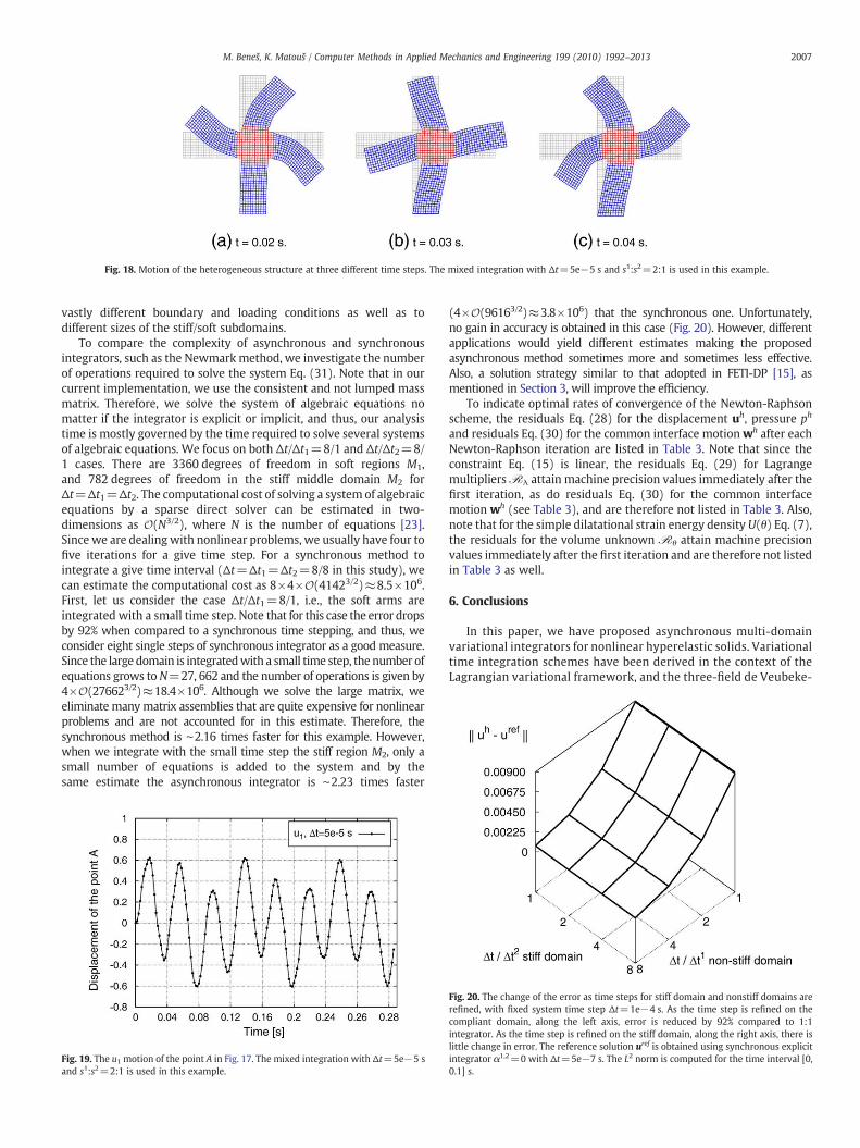


![[Muon LFV-1 2] Review - KEKresearch.kek.jp/group/fapps09/program/Muon_LFV2/Muon_LFV...(Lagarrigue and Peyrou, 1952). Such searches were sig-nificantly improved when muons became artificially](https://static.documents.pub/doc/80x56/5e999036c705fa4795669ebc/muon-lfv-1-2-review-lagarrigue-and-peyrou-1952-such-searches-were-sig-niicantly.jpg)


