COMPUTER PROGRAMS IN SEISMOLOGY - Department of … · 2011-07-07 · PREFACE Preparing the latest...

COMPUTER PROGRAMS IN SEISMOLOGY

AN OVERVIEW OF SYNTHETICSEISMOGRAM COMPUTATION

Robert B. HerrmannEditor

Professor of GeophysicsDepartment of Earth and Atmospheric Sciences

Saint Louis University

Version 3.302002

Copyright © 2002 by R. B. Herrmann

Version 3.30 17 September 2006

-2-

Contents

Preface vi

Chapter 1: DataFormats1. Introduction 1-12. Earth Model 1-23. Time histories 1-44. Distance File 1-85. Depth File 1-96. SURF96 1-107. SAC 1-11

Chapter 2: Generalized Ray1. Introduction 2-12. gprep96 2-13. genray96 2-44. gpulse96 2-55. Sample Run 2-8

DRAFT iii 17 September 2006

Chapter 3: Wav enumber Integration1. Introduction 3-12. hprep96 3-13. hspec96 3-44. hpulse96 3-55. Sample Run 3-66. hwhole96 3-77. hspec96p 3-9

Chapter 4: Modal Summation1. Introduction 4-12. sprep96 4-13. sdisp96 4-34. scomb96 4-45. slegn96/sregn96 4-56. spulse96 4-77. sdpsrf96 4-88. sdpegn96 4-109. sdpder96 4-1210. sdpdsp96 4-1311. sdprad96 4-1412. Sample Runs 4-1513. Dispersion Repair 4-23

DRAFT iv 17 September 2006

Chapter 5: Asymptotic Ray Theory1. Introduction 5-12. cprep96 5-13. cseis96 5-34. cpulse96 5-45. cray96 5-66. Sample Run 5-77. Laterally Varying Models 5-11

Chapter 6: File96 Filters1. Introduction 6-12. fmech96 6-13. fbutt96 6-34. ffilt96 6-55. finteg96 6-86. fderiv96 6-97. fsel96 6-108. fplot96 6-119. fplotg96 6-1210. fprof96 6-1411. fplot396 6-1512. fspec96 6-1913. fdecon96 6-20

DRAFT v 17 September 2006

Chapter 7: SAC Filters1. Introduction 7-12. sactoasc 7-13. asctosac 7-14. shwsac 7-25. f96tosac 7-46. sactof96 7-67. sacdecon 7-78. saciterd 7-89. sacevalr 7-1110. saclhdr 7-1211. sacfilt 7-1412. saccvt 7-15

Chapter 8: Earth Model Files1. Introduction 8-12. model96 8-13. shwmod96 8-14. timmod96 8-25. mkmod96 8-36. time96 8-57. refmod96 8-68. prfmod96 8-7

DRAFT vi 17 September 2006

Chapter 9: Transverse Isotropy1. Introduction 9-12. TI model 9-23. tmkmod96 9-44. is2timod 9-55. ti2ismod 9-66. tshwmod96 9-77. tspec96 9-108. tspec96p 9-139. trftn96 9-1610. tfmech96 9-1711. Limitations and Directions 9-19

Appendix A: CALPLOT Graphics1. Introduction A-12. PostScript Output A-23. Windows Screen Output A-54. Tektronix Output A-75. X11 Output A-86. PNG Output A-117. Figure Manipulation A-128. CALPLOT Colors A-15

Appendix B: Green's Functions1. Introduction B-12. Combinations of Green's Functions B-23. Time Functions B-64. Pulses B-95. References B-11

DRAFT vii 17 September 2006

Appendix C: Program Limitations1. Introduction C-12. Volume II C-13. Volume III C-14. Volume IV C-15. Volume V C-26. Volume VI C-27. Earth Models C-2

Appendix D: Work to Do1. Introduction D-1

Appendix E: Installation1. Introduction E-1

DRAFT viii 17 September 2006

DRAFT ix 17 September 2006

PREFACE

Preparing the latest version of Computer Programs in Seismology included a majoreffort toward making the programs easier to use. This is done in part by reducing thenumber of programs in the distribution andeliminating those designed for algorithm ver-if ication. The choice of programs to eliminate was based on the usage of programs duringthe past decade. Another change was an effort to provide consistency in file formats andcommand line flags.

In this volume I describe programs used for synthetic seismogram generation. Simpleflowcharts are given to indicate the logical flow and the program output. The followingsymbols are used:

data format

program

other output/input

processing flow

optional processing flow

Since the programs will be run on UNIX and MSDOS systems, command line redirectionin place of terminal entry is used to read data into the program from a file. Thisstandardentry in the C language isstdin. The corresponding standard program output isstdout.This terminology will be used in flow charts. Acircle with stdin indicates input from aterminal or from a file using the input redirection, and a circle withstdout indicates out-put to the terminal, or output to a user file using output redirection. A simple instance ofredirection is

Version 3.30 vi 17 September 2006

rbh> program < input_file > output_file

Here, as in all examples, therbh> indicates a command line prompt. This program usagewill be represented in a flow diagram as

stdin

program

stdout

Even though almost all programs are written in FORTRAN, ASCII files that are usedfor standard data formats are defined to be parsed. Thus, if several numbers are writtenper line, they will be separated by white space. In addition, if an array is written, e.g., atime series with fiv e values per ASCII line, then the last entry will be zero filled so that aconsistent C format can be used, e.g., " %f %f %f %f %f ".

A reference to a specific documented program or file format is indicated in bold, e.g.,genray96. Specific input/output files are indicated in italic, e.g.,RAY96.PLT. Terminalinput/output is indicated by a courier font, e.g.,

genray96 -d dfile .

I begin with a discussion of data formats, followed by a discussion of individual pro-grams for generating synthetic seismograms.

Finally, I describe the program usage, but the leave detailed documentation in themanual pages for the individual volumes. In addition, the ultimate source of what a pro-gram can do is the actual source code.

Version 3.30 vii 17 September 2006

Computer Programs in Seismology - Overview

Computer Programs in Seismology 3.1

I hav eusedComputer Programs in Seismology 3.0during the past four years andhave found and corrected many inconsistencies. So how does version 3.1 differ, otherthan the bug fixes. Thesignificant answer is that this version is upwardly compatiblewith the Version 3.0. The intermediate binary file format for synthetic seismograms is notcompatible, though.

• Two blank fields in thefi le96(V) trace file format are now used:LINE13 now con-tains the model predicted P, SV and SH travel times which will be used to align syn-thetics and observed data for wav eform inversion; LINE14 contains medium parame-ters at the source, corresponding the the Love (1944) A, C, F, L and N constants for atransversely anisotropic medium.In addition the timing information, sample interval,have an expanded format to permit travel times in the microsecond range, which isnecessary for experimental measurements at very short distances in engineering andmedicine.

• New utility programs: saclhdr(V), fdecon96(V), fspec96(V), sacfile(V) and sace-valr(V) . In addition, improved subroutine libraries leads to uniform graphics for allroutines.

So what will the next version entail? There will be full support for transverse anisotr-poic media in the wav enumber integration and mode code.Wa ve propagation in a gravi-ating fluid may also be in Version 3.2. Version 3.2 will also see the the first set of pro-grams for analyzing data.

R. B. HerrmannSaint Louis UniversityJanuary 15, 2001

Version 3.30 viii 17 September 2006

CHAPTER 1DATA FORMATS

1. Introduction

The focus of the previous version ofComputer Programs in Seismology was theimplementation of specific algorithms for the analysis of seismic data. Little effort wasdirected toward developing a consistent set of input and output files for these programs.The focus was on specific volumes for each algorithm.

The use of these programs for the analysis of seismic data identified that more focusshould be placed on data/model formats rather than on the algorithms. The two basicfi les used for all synthetic seismogram computations are the earth model file and the out-put time history. Thus the user will find the programs easier to use if different algorithmscan be run using the same input and output formats. The specification of these file for-mats is complicated by the many different ways the earth models can be described andseismic data can be stored.

All programs described here will use amodel96earth model description and will cre-ate a time history in thefi le96 format. The earth model format is well defined for layeredisotropic media, but is general enough to encompass other more complicated models. Theoutput file format is general enough for the present uses of data, can be converted easilyto other formats, and can be extended in the future. The basis of this flexibility is the useof keyed comment lines at the head of each file and the allowance for future extension.

An example of how this concept works is given in Figures 1 and 2. Figure 1 indicatesthat the same earth model file can be used to generate synthetic seismograms by general-ized ray, model summation or wav enumber integration. Figure2 indicates that certain fil-tering operations have been designed to operate onfi le96(V) fi les.

Version 3.30 1-1 17 September 2006


model96

gprep96 genray96 gpulse96

Generalized Ray

hprep96 hspec96 hpulse96

fi le96

Wa venumber Integration

hprep96p hspec96p hpulse96

p-τ

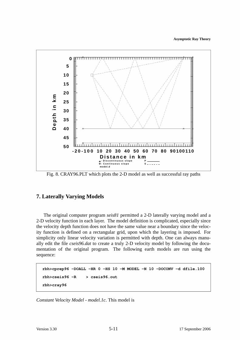
cprep96 cseis96 cpulse96

Asymptotic Ray Theory Ray

sprep96 sdisp96slegn96

sregn96spulse96

Modal Summation

Fig. 1. Processing flow for synthetic seismogram programs.

fi le96

fmech96

fi le96

fbutt96

finteg96

fderiv96

ff i lt96fsel96

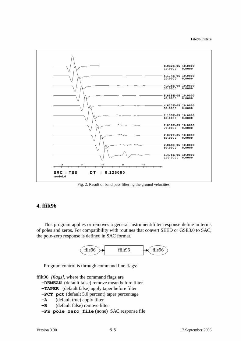
Fig. 2. Filtering operations.

2. Earth Model

A model96model file consists of eleven ASCII header lines followed by the detailedmodel. An example is the best way to present this concept. The model shown below is fora flat, isotropic, flat-layered, constant velocity earth.


Data Formats

MODEL.01TEST MODELISOTROPICKGSFLAT EARTH1-DCONSTANT VELOCITYLINE08LINE09LINE10LINE11

H VP VS RHO QP QS ETAP ETAS FREFP FREFS40. 6.0 3.5 2.8 0.0 0.0 0.0 0.0 1.0 1.000. 8.0 4.7 3.3 0.0 0.0 0.0 0.0 1.0 1.0

The context of the lines in this example are as follow:

Line 01: Thefirst line requires the use of the keyword MODELwhich identifies this ASCIIfi le as an earth model file. This keyword is absolutely necessary. In thisexample the keyword isMODEL.01 indicates that the format is Version 01.

Line 02: Thesecond line is a descriptive comment for the model. Its only limitation isthat it can be no more than 80 characters long.

Line 03: Thethird line describes the isotropy of the medium. The allowed keywords areISOTROPIC, TRANSVERSE ISOTROPICandANISOTROPIC. All pro-grams inComputer Programs in Seismology will work with the ISOTROPICdesignation.

Line 04: Thefourth line indicates the model units.KGSindicates that the distances, layerthicknesses are inkilometers, velocities are inkilometers/second, the densityis in gm/cm3, and that time is inseconds. The units are necessary for definingsynthetic seismogram amplitudes.

Line 05: Thefifth line uses the key wordsFLAT EARTHor SPHERICAL EARTH.

Line 06: Thesixth line describes the nature of model boundaries, e.g.,1-D , 2-D , or 3-D ,

Line 07: Theseventh line describes the nature of layer velocities, e.g.,CONSTANTVELOCITYor VARIABLE VELOCITY .

Lines 08-11: Theeighth througheleventh lines are positions left for future extension inthe file format.

Remaining Lines: The remaining lines are specific to a particular model format.

For an isotropic, one-dimensional medium with constant velocity, the earth modelconsists of a sequence of flat layers in theFLAT EARTH or spherical shells in theSPHERICAL EARTH. The first line of this model definition is an ASCII string



indicating column headings.This is permitted for readability, but the order of the actualnumerical entires is fixed. Theremaining lines specifically define the model. The modelis described in free format by 10 columns:

H VP VS ρ QP QS ηP ηS fP fS

where His the layer thickness, with the bottom layer thickness being 0 or more kilome-ters. IfH is neg ative at the top of the layer stack, then this will define a reference level ofthe surface (this will facilitate studying earth - atmosphere interaction).VP and VS arethe compressional and shear wav evelocities in each layer, and ρ is the layer density. Theanelastic attenuation model is described in terms of three parameters:Qv, ηv and fv,where vis eitherP or S. For wav etype v, the specific quality factor as a function of fre-quency f is giv en by Qv(f ) = Qv(f / fv)

ηv .

In the computer programs,Q < 1 is never permitted, which is not an unreasonableassumption. Thus the earth model may be given in terms ofQ or Q−1, since the programswill automatically associate a value <1 as being Q−1 and a value >1 as being Q. This willmake data input easier.

Finally, the documentation of a specific program will indicate the suite of models thatcan be considered.

To assist in creating the file correctly, Chapter 8 discusses the programmkmod96.

3. Time histories

Time histories are stored in thefi le96 format. Earlier versions of the package had twotime history formats: one for Green’s functions of synthetic seismograms, and other forthree-component time histories. Because of this, it was necessary to have duplicates ofalgorithms, e.g., integration, filtering or differentiation, to act on the two time history for-mats. Thisled to a set of programs differing only in input/output formats.

Other seismological formats exist. The SAC format file consists of a single trace,which can be inconvenient and inefficient for storing Green’s functions, or typical three-component seismic time histories. Both SAC headers and the CSS data base provideinformation about many aspects of the time history, whereas the earlier versions of thispackage did not.

The approach taken here is to implement general purpose programs that work ontime histories, irrespective of the specific time history format. Thus one will be able to fil-ter or display Green’s functions or specify a source mechanism to convert the Green’sfunctions to a three-component time history and then filter or display the traces, using thesame programs.

The cost for generality is a slightly more complicated file format,fi le96.

Consider the following example:

The format consists of two sections: a station header and specific traces, each ofwhich has an individual trace header as well as the trace itself. The meaning of the linesin this example are as follow:


Data Formats

FILE21.02SYNTHETICTIME_DOMAINCOUNTSNone

0 0 0 0 0 0 .0000 0.000000 0.000000 10.000000GRN16

0.000000 0.000000 0.00010.0000 0.0899 0.0000 180.0000

Nonemodel.dPa

2.357022524 4.040610313 4.0406103130.1008E+03 0.1008E+03 0.3220E+02 0.3430E+02 0.3430E+02 0.2800E+01

LINE15LINE16

1 4 1 4 5 1 4 5 1 4 1 4 1 4 5 0 0 0 0 0 0ZEX

-90.000 0.000 0.125 20 0 0 0 0 0 .6667

0.00000000E+00 0.00000000E+00 0.00000000E+00 0.00000000E+00REX

0.000 0.000 0.125 20 0 0 0 0 0 .6667

0.00000000E+00 0.00000000E+00 0.00000000E+00 0.00000000E+00ZVF

-90.000 0.000 0.125 20 0 0 0 0 0 .6667

0.00000000E+00 0.00000000E+00 0.00000000E+00 0.00000000E+00RVF

0.000 0.000 0.125 20 0 0 0 0 0 .6667

0.00000000E+00 0.00000000E+00 0.00000000E+00 0.00000000E+00ZHF

-90.000 0.000 0.125 20 0 0 0 0 0 .6667

0.00000000E+00 0.00000000E+00 0.00000000E+00 0.00000000E+00RHF

0.000 0.000 0.125 20 0 0 0 0 0 .6667

0.00000000E+00 0.00000000E+00 0.00000000E+00 0.00000000E+00THF

0.000 90.000 0.125 20 0 0 0 0 0 .6667

0.00000000E+00 0.00000000E+00 0.00000000E+00 0.00000000E+00

Station Header

Line 01: Thefirst line requires the use of one of the following keywords: FILE01.02 ,FILE03.02 , or FILE16.02 , which uniquely defines the file as being ageneral time series format. The keywords indicate that the ASCII file is a sin-gle component, three component or sixteen component time history,



respectively. In the case of multiple components, not all need be present, asin the case of only transverse component Green’s functions. The.01 exten-sion indicates the version number of the current format definition, with thecurrent version being 01. One of these keywords is required.

Line 02: Thesecond line requires the use of one of the two keywords: OBSERVEDorSYNTHETIC. This is used to identify the origin of the trace, and also toresolve issues concerning the time of the first sample.One of thesekeywords is required.

Line 03: Thethird line requires the use of one of the two keywords: TIME_DOMAINorFREQUENCY_DOMAINto indicate whether the series is a time series or acomplex Fourier spectra. At present, only theTIME_DOMAIN is imple-mented. Oneof these keywords is required.

Line 04: Thefourth line indicates the units of the time series.For TIME_DOMAINthecurrent options areCOUNTS, CM, CM/SEC, CM/SEC/SEC, M, M/SEC,M/SEC/SEC, MICRON, MICRON/SEC, or MICRON/SEC/SEC, One ofthese keywords is required.

Line 05: Thefifth line is a comment string of no more than to 80 characters in lengthdescribing the filtering operations performed on the data stream.If no pro-cessing has been done, the keyword isNONE.

Line 06: Thesixth line information on the event origin, if known. Theentries in spaceseparated free format areYEAR(an integer, e.g., 1990),MONTH(an integer, e.g., 12),DAY(an integer, e.g., 28),HOUR(an integer, e.g., 13),MINUTE(an integer, e.g., 6),SECOND(a float, e.g., 23.345),EVENT_LATITUDE(a float, north = positive),EVENT_LONGITUDE(a float, east = positive), andEVENT_DEPTH(a float, positive = down).For SYNTHETIC, all entries are zero, exceptEVENT_DEPTH.

Line 07: Theseventh line provides informationon the station name. The line consists ofa character string for the station name:STATION_NAME(character*8),For SYNTHETIC, STATION_NAMEis GRN16,

Line 08: Theeighth line provides information the station location. Space separated freeformat is used. The order of entries on the line areSTATION_LATITUDE (a float, north = positive),STATION_LONGITUDE(a float, east = positive),STATION_ELEVATION(a float in kilometers, positive = up).


Data Formats

For SYNTHETIC, STATION_LATITUDE andSTATION_LONGITUDEare0.0, andSTATION_ELEVATION is receiver depth in kilometers (down ispositive).

Line 09: Theninth line provides information about the position of the station with respectto the source, if known. Theentries in space separated free format areDISTANCE_KILOMETERS(distance between source and receiver,DISTANCE_DEGREES(distance in degrees, roughly 111.195°/km)STATION_EVENT_AZIMUTH(azimuth in °, North=0, East= 90)EVENT_STATION_AZIMUTH(back azimuth in °, North=0, East= 90).All four fields are required.

Line 10: Thetenth line is a comment string up to 80 characters in length describing thesource pulse used in making the synthetic seismograms.If no convolutionwith a source time function has been performed, the keyword NONEis used.

Line 11: Theeleventh line is a comment line. For SYNTHETICtime histories this will bethe name of the earth model file.

Line 12: Thetwelvth line indicates the units of the pressure or stress time series.The cur-rent options arePa, MPa, One of these keywords is required.

Line 13: Thethirteenth line gives the model predicted ray theory first arrival times of P,SV and SH for the model. If these are not defined, each is set to-12345.0,which is SAC syntax for an undefined number. The purpose of this field is tobe able to define the first arrival times in the SAC file for use in sourceparameter inversion.

Line 14: Thefourteenth line gives the model predicted medium parametersA, C, F, L, Nand ρ at the source depth. These are the fiv e medium parameters for a trans-versely isotropic medium with vertical axis of symmetry and the density. Foran isotropic medium,A = C = λ + 2µ, F = λ , and L = N = µ. The units chosedhere assume that the corresponding wav evelocty is inkm/sec and the densityis gm/cm3. If the the data file corresponds to observed and not synthetic timeseries, or if these are not defined, then all six parameters are set to 0.0!

Lines 15-16: Thefifteenth throughsixteenth lines are positions left for future expansionof the file format.

Line 17: Theseventeenth line consists the of theJSRC array of 21 integers. The purposeof this array is twofold.

First, if thei’th trace does not exist, or is not generated, thenJSRC(i) = 0 .This makes this ASCII file smaller in size since only non-zero tracesarestored.

The second purpose is to identify the trace type, e.g., 1 = Z (vertical), 2 = N



(north), 3 = E (east), 4 = R (radial), 5 = T (transverse), and 6 = O (other).This second purpose is only introduced to make later manipulation of traceseasier. The ultimate definition of trace orientation is in the individual traceheader.

Tr ace Header and Trace

There are a maximum of 1, 3 or 16 traces associated with theFILE01 , FILE03 orFILE16 keywords, respectively. The presence of a trace is indicated by theJSRC(i) ≠ 0flag in the Station Header. Each trace description consists of a three line header followedby the traces.

Line 01: Thefirst line contains a character string for the component name:COMPONENT_NAME(character*8),

Line 02: Thesecond line gives component orientation and sampling information:COMPONENT_INCIDENCE(float that describes the angle of positive motionwith respect to the vertical. A value of -90 indicates up, 0 indicates horizon-tal, and 90 indicates down)COMPONENT_AZIMUTH(float that describes horizontal orientation of posi-tive motion, e.g., 0 is north, 90 is east)COMPONENT_SAMPLE_INTERVAL(float describing sampling interval inseconds),COMPONENT_NUMBER_OF_SAMPLES(integer)

Line 03: Thethird line uses space separated free format to define the time of the firstsample:YEAR(an integer, e.g., 1990),MONTH(an integer, e.g., 12),DAY(an integer, e.g., 28),HOUR(an integer, e.g., 13),MINUTE(an integer, e.g., 6),SECOND(a float, e.g., 23.345),

Remaining Lines: The remaining lines consist of the trace written in the FORTRAN for-mat (e16.8,1x,e16.8,1x,e16.8,1x,e16.8). There are four entries per line. Ifnumber of points is not a multiple of 4, then the line is zero filled. (Bewareof differences in the E notation in FORTRAN and C for different compilers.In FORTRAN on usually will see and entry like +1.000E+21 and in C anentry like +1.000E+021. This make cause difficulty if the user attempts toduplicate this format in C.)

4. Distance File


Data Formats

This file defines characteristics of the time series to be created. It consists of fiv eASCII entries per line in free format. These entries are

DIST DT NPTS T0 VRED

whereDIST is the desired epicentral (horizontal distance) from the source to the receiver,DT is the sampling interval in seconds,NPTSis the number of samples which must be apower of 2 (note the programs will automatically check this), and the time of the firstsample is

T0 + DIST/VRED seconds. IfVRED = 0 , then the time of the first sample isT0.For use by 2-D ray tracing programs,DIST can be negative.

This issue of distance may be revisited later when 2-D models are fully incorporated,since one may wish to specify the horizontal position of the source as well as the receiver.

Some programs, e.g.,hprep96(VI) andhprep96p(VI), will read the distance file inits entirety and attempt to determine a commonDT, usually the smallest, andNPTS, usu-ally the largest. The time series output values ofDT andNPTSmay thus differ from thatrequested. Thisis because of the need to sample exactly the same frequencies for all dis-tances. If this result is not desired, the user should execute the programs separately foreach distance.

A sample distance file is

10.0 0.125 256 -1.0 6.020.0 0.125 256 -1.0 6.030.0 0.125 256 -1.0 6.040.0 0.125 256 -1.0 6.050.0 0.125 256 -1.0 6.060.0 0.125 256 -1.0 6.070.0 0.125 256 -1.0 6.080.0 0.125 256 -1.0 6.090.0 0.125 256 -1.0 6.0

100.0 0.125 256 -1.0 6.0

5. Depth File

This file defines the source or receiver depths in the case that synthetics for more thana single depth are to be generated.In the programshprep96(VI) for wav enumber inte-gration, andhprep96p(VI) for p-τ response, multiple depths for source or receiver isindicated by the command line flags-FHS source_depth_file or -FHRreceiver_depth_file , respectively.

The contents of the depth file consist of a single ASCII entry per line in free formatgiving the depth:



depth

A sample depth file is

0.02.55.07.5

10.012.515.017.520.0

6. SURF96

The surf96 format is used for experimental dispersion data and is generated by theprogramsdpegn96and used bysdpegn96andsdpdsp96. The format is very simple:

SURF96 WAVE TYPE FLAG MODE PERIOD VALUE DVALUE.... .... .... .... .... ... ....

SURF96 WAVE TYPE FLAG MODE PERIOD VALUE DVALUE

where

SURF96 a left-justified keyword,WAVE single characterR i L for Rayleigh or LoveTYPE single characterC, U, or G for the observed phase velocity, group velocity

or gammaFLAG single characterX for observed orT for theoretical value. This distinction

is used in plotted theoretical dispersion curves and observed dataMODE mode of observation:0 is fundamental mode,1 is 1stPERIOD period of observation in units ofsecondsVALUE observed dispersion in units forkm/sec for Cor Uor km-1 for GtypeDVALUE error in observed value. Note for synthetics, this is set to a small value of

0.001 for velocity and0.0000001 for gamma. For observed data, these val-ues should be be standard error of the mean and not the standard error ofthe observation.

A sampleSURF96dispersion file is

SURF96 R C X 0 5.0000 3.2044 0.10000E-02SURF96 R U T 0 5.0000 3.0707 0.10000E-02SURF96 R G T 0 5.0000 0.31785E-03 0.10000E-06SURF96 L C T 0 8.0000 3.6255 0.10000E-02SURF96 L U T 0 8.0000 3.4402 0.10000E-02


Data Formats

SURF96 L G T 0 8.0000 0.16573E-03 0.10000E-06

As with all formats, except theDepth File format, the keywords are a required part of thefi le definition. In addition theL, R, C, U and G codes are used for benefit of peopleand not computers.

7. SAC

SAC is a standard trace analysis package for manipulating time series.ComputerPrograms in Seismology.

Several conversion programs, described in detail in Chapter 6, were written to workwith SAC files:

sactoasc - convert SAC binary to SAC ascii formatasctosac - convert SAC ascii to SAC binary format

This is useful in transferring SAC files between machines of different binary archi-tecture.

shwsac - reads a SAC binary file, shows all header variables, and lists ten representativevalues of the times series.

f96tosac - convert fi le96(V) to SAC binary formatsactof96 - convert SAC binary tofi le96(V) formatsaclhdr - list the SAC header value for use in SHELL scripts.sacdecon - a water level deconvolution program using SAC files.saciterd - iterative time domain deconvolution program using SAC files.sacevalr - instrument response deconvolution using amplitude and phase response

fi les generated by the IRIS programevalresp.sacfilt - apply or remove a filter response defined by a SAC pole-zero filesaccvt - convert SAC file from big-endian (SPARC) to little-endian (INTEL) and vice

versa.



CHAPTER 2GENERALIZED RAY

1. Introduction

model96

gprep96

genray96

gpulse96

fi le96

In this chapter I describe the use of generalized rays forthe generation of synthetic seismograms. This type of seis-mogram synthesis is very efficient if only a few raysbetween the source and receiver are required in simple lay-ered media. The difficulties in using more rays for adetailed structure are twofold. First, the ray description istedious, since the program requires each ray segment to bedefined in terms of ray type.The second problem is thatcomputations with many rays may take much longer thanusing modal summation or wav enumber integration tech-niques.

To address the first problem, the programgprep96 isused to automatically generate the ray description file. Thisoutput is then used by the programgenray96 to computethe medium response.The output ofgenray96 is in thefi le96 Green’s function format, but convolution with thesecond derivative of the source time function is done by theprogramgpulse96.

2. gprep96

The generalized ray technique requires the complete specification of a ray pathbetween the source and receiver. This means that one must know whether the ray leavesthe source in an upward or downward section, the layer in which each segment of the raylies, and the wav etype itself for each segment, e.g., P, SV or SH. Such descriptions arenot difficult for a simple model with few conversions upon reflection and transmissionbetween P and SV, but become laborious for more complicated models. In addition,changing the layer in which either the source or receiver lie requires a completely



different ray specification.

The programgprep96 automatically provides the ray specifications for all raysbetween the source and receiver in a manner that makes it trivial to change source orreceiver depths. The secret of the ray generation is to change the point of view from thatof rays in layers to one of rays interacting at layer boundaries, with the source andreceiver occupying pseudo-boundaries. With this convention, a ray may leave the sourcegoing upward (0) or downward (1). The ray may next interact with the adjacent boundary,going either up (0) or down (1). This quickly suggests the use of a binary number systemto represent a ray path. If the ray has two segments or legs after leaving the source, thenthere are four possible rays. Figure 1 illustrates this.

*

0

1

00

01

10

11

Fig. 1. Simple ray descriptions.

In this picture 4 rays can be represented by two segments. Since a 4 byte integer isused to represent the unique rays ingprep96, there can be there can be up to232 possiblerays, e.g., 2 with one segment, 4 with two segments, ...,231 with 31 segments. Themini-mum number of segments is the direct ray path between the source and the receiver. If aray path extends above the top or below the bottom of the model, the particular path isignored.

Once a ray path is determined, each ray segment can systematically take on 2 values,e.g., P or SV, leading to yet another set of combinations. The maximum number of P-SVsegments, permitting conversion upon reflection and refractions, is432, which is signifi-cantly more than one would ever desire to run.

The large number of possible total rays, as well as the use of a 32 bit integer, meansthat one may never wish to consider a model with many layers. For example, it would beimpossible to use this program with a fifty layer model, with the source and receiver atopposite ends of the model, since 50 segments would be required just for the direct rayand only 31 segments are permitted using the 4 byte representation of integers.

Figure 2 shows the processing flow for this program. The program requires one earthmodel file in themodel96 format and two optional control files. The output consists ofthe file GPREP96.PLT, a CALPLOT(I) graphics file, the file genray96.ray, the ray con-trol file for genray96(V), and screen output designated bystdout.


Generalized Ray

Program control is through the command line:

gprep96 [flags], where the command flags are-M model - model is a file in themodel96format. Thisis required.-DOP-DOSV-DOSH-DOALL

One or more of these must be specified. These tell the program to compute P, SV,SH and all ray segments. If for example, no SH is desired but both P and SV aredesired, then use-DOP -DOSV. If only -DOP is specified, then there will be no P-> SV or SV -> P conversions.

-DOREFLPermit P-SV conversions only upon reflection, otherwise reflections will only be P→ P SV → SV.

-DOTRANPermit P-SV conversions only upon transmission, otherwise transmissions willonly be P→ P SV → SV.

-DOCONVPermit P-SV conversions on both reflection and transmission

The default is that no conversions are computed.-DENY deny_file

A simple listing of interfaces at which only transmission without wav etype conver-sion is permitted. Reflections are denied at this boundary. The file consists of a sin-gle entry per line, giving the specific boundary number of the earth model. Thismay be useful to approximate a gradient when there are no turning rays.

-R reverberation_fileA simple listing of layers and the maximum number of ray segments in a layer.This is useful to focus on the reverberations within specific layers. The default is topermit as many as possible.

-N maximum_number_of_segmentsThe maximum number of ray segments permitted in the ray description. Since arti-ficial boundaries are inserted at the source and receiver depths, this number must belarge enough to permit one direct ray between the source and receiver.

-HS source_depthThe depth of the source in the model

-HR receiver_depthThe depth of the receiver in the model

-?-h

Online help



gprep96

stdout genray96.rayGPREP96.PLT

model96 deny reverb

Fig. 2. Processing flow for gprep96

3. genray96

genray96creates the synthetic seismogram by applying the Cagniard-de Hoop tech-nique to each ray description. This technique is well described in seismological litera-ture. Thisprogram is a modification of a program originally developed by Dr. C. A.Langston, The Pennsylvania State University, in the late 1970’s.

Figure 3 shows the processing flow for this program. The program requires one earthmodel file in themodel96format which is referenced through the file genray96.ray gen-erated bygprep96(V). The other required input file is adistance_file described in Chap-ter 1. The output consists of the file genray96.grn in thefi le96(V) format, a tabulation oftravel time for each ray description in the file genray96.tim and screen output designatedby stdout.


genray96 [flags], where the command flags are-ALL

Compute all Green’s functions(default true).-EQEX

Compute only Green’s functions for moment tensor sources.(default false)


Generalized Ray

-EXFComputer Green’s functions for explosion and point forces. This addresses explo-ration sources.(default false)

-d dfileThe required distance file. The file contains the following ASCII entries per line:


whereDIST is the epicentral distance in kilometers,DT is the sampling interval forthe time series,NPTSis the number of points in the time series ( a power of 2). T0and VREDare used to define the time of the first sample point which isT0 +DIST/VRED if VRED ≠ 0 or T0 if VRED = 0 .

This file is required-n nasym

Number of asymptotic terms to use from the expansion of the modified Besselfunction Km(spr). If nasym = 1, near-field contributions are not included.Theeffect of this term can be seen in Helmberger and Harkrider (1978).(defaultnasym= 1)

-SUOnly produce Green’s functions for rays that leave the source upward.

-SDOnly produce Green’s functions for rays that leave the source downward.

-SPUPOnly produce Green’s functions for P rays that leave the source upward.

-SSUPOnly produce Green’s functions for S rays that leave the source upward.

-SPDNOnly produce Green’s functions for P rays that leave the source downward.

-SSDNOnly produce Green’s functions for S rays that leave the source downward.(If none of these flags are given, the synthetic will consist of all rays from thesource)

-TIMEDo not produce the Green’s functions. Just create the file genray96.tim which con-tains travel time information.

-va -vb -vc -vd -ve -vf -vg -vhVarious flags to output intermediate results. Used as a debugging tool. Onlyattempt to use this with theory and source code at hand.

-?-h

Program does nothing, other than to list the command line flags.

4. gpulse96



genray96

stdout genray96.grngenray96.tim

model96 dfile genray96.ray

Fig. 3. Processing flow for genray96

Figure 4 shows the processing flow for this program. The program requires thegen-ray96.grn fi le created bygenray96(V) and optionally the source pulse definition filerfile. The program output is onstdout and is a time series infi le96(V) format. SeeAppendix B concerning the Green’s functions.


gpulse96 [flags], where the command flags are-v

Verbose output-t

Triangular pulse of base 2 L∆t, which∆t is the sample interval. To avoid problemswith sharp truncation in the frequency domain spectra by sampling, never set L < 2.The special case of L = 2 for the triangular pulse is equivalent to the parabolicpulse with L = 1.

-pParabolic Pulse of base4 L ∆t

-oOhnaka pulse with parameter alpha

-i


Generalized Ray

Dirac Delta function-l L

Source duration factor for the parabolic and triangular pulses.-a alpha

Shape parameter for Ohnaka pulse-D

Output is ground displacement-V

Output is ground velocity (default)-A

Output is ground acceleration-F rfile

User supplied pulse-m mult

Multiplier (default 1.0)-OD

Output is forced to be named displacement-OV

Output is forced to be named velocity-OA

Output is forced to be named acceleration-Z zero phase triangular/parabolic pulse, else causal

-?-h

Online help concerning program usage



gpulse96

stdoutfi le96

genray96.grnrfile

Fig. 4. Processing flow for gpulse96

5. Sample Run

Given the sample model and distance files of Chapter 1, the following commands arerun:

rbh> gprep96 -DOALL -HR 0 -HS 10 -M model.d -N 10 -DOCONV

rbh> genray96 -d dfile > genray96.out

rbh> gpulse96 -V -p -l 4 | f prof96

The graphics output ofgprep96 is given in Figure 5.


Generalized Ray

TEST MODEL DEPTH SRC=1 0 . 0 0 0 REC=0 . 0 0 0

H VP VS RHO

4 0 . 0 0 0 6 . 0 0 0 3 . 5 0 0 2 . 8 0 0

1

1000

REC

( 0 . 0 0 0 )

SRC

( 1 0 . 0 0 0 )

0 . 0 0 0 8 . 0 0 0 4 . 7 0 0 3 . 3 0 0

2

model .dARTIFICIAL BOUNDARY FOR SOURCE-RECEIVERLAYER BOUNDARYLAYER BOUNDARY (NO CONVERSIONS)

Fig. 5. The GPREP96.PLT generated.

The synthetic transverse time histories for a vertical strike-slip source are given in Figure6.



1 0 . 0 0 0 00 . 0 0 0 0

1 . 2 0 5 E - 0 41 0 . 0 0 0 0

1 0 . 0 0 0 00 . 0 0 0 0

8 . 3 5 9 E - 0 52 0 . 0 0 0 0

1 0 . 0 0 0 00 . 0 0 0 0

5 . 8 0 2 E - 0 53 0 . 0 0 0 0

1 0 . 0 0 0 00 . 0 0 0 0

7 . 7 4 7 E - 0 54 0 . 0 0 0 0

1 0 . 0 0 0 00 . 0 0 0 0

6 . 3 0 9 E - 0 55 0 . 0 0 0 0

1 0 . 0 0 0 00 . 0 0 0 0

2 . 8 2 3 E - 0 56 0 . 0 0 0 0

1 0 . 0 0 0 00 . 0 0 0 0

2 . 6 7 6 E - 0 57 0 . 0 0 0 0

1 0 . 0 0 0 00 . 0 0 0 0

2 . 7 5 9 E - 0 58 0 . 0 0 0 0

1 0 . 0 0 0 00 . 0 0 0 0

2 . 7 2 0 E - 0 59 0 . 0 0 0 0

1 0 . 0 0 0 00 . 0 0 0 0

1 . 9 5 6 E - 0 51 0 0 . 0 0 0 0

18 24 30 36 42

SRC = TSS D T = 0 . 1 2 5 0 0 0model .d

Fig. 6. The TSS time histories file generated byfprof96.


Generalized Ray

CHAPTER 3WAVENUMBER INTEGRATION

1. Introduction

model96

hprep96

hspec96

hpulse96

fi le96

This chapter describes the use of wav enumber integra-tion for the generation of synthetic seismograms. This typeof seismogram synthesis is complete, but can be computa-tionally intensive. There are three stages between the speci-fication of the model file and the final synthetic seismo-grams.

The programhprep96 creates a data file hspec96.datfor use byhspec96to create the Green’s functions in theω -distance space. The output of this program is a binaryfi le, hspec96.grn, which is used byhpulse96 to convolvethe response with the source time function to createfi le96Green’s function time histories.

2. hprep96

The purpose of this program is to generate a data file for use by the wav enumber inte-gration programs. These programs are more general than the generalized ray programs inthat one may consider more than a single distance, source depth or receiver depth. Thispermits creating record sections for vertical seismic profiling as well as ordinary refrac-tion lines. However there is the requirement to compute synthetics using the same numberof points, N, and the sample time domain sampling interval∆t.

To generate synthetics as free as possible from numerical artifacts, due to the time andspace domain periodicity caused by sampling in the frequency - wav enumber domain,certain parameters must be carefully defined. These areα and L.α is used to alleviate thetime domain periodicity, and should be such thatα N∆t ≈ 2. 5, which usually works wellunless the layer multiples do not decay rapidly. This default choice ensures that arrivalsthat wrap around to interfere with the desired signal are reduced by a factor ofe2. 5. Thewavenumber sampling is∆k = 2π / L, where theL parameter is defined using the criteria



developed by Bouchon.

This program will read a model, the distance file, and get source and receiver depthinformation from the command line, and will generate the data file required by thewavenumber integration programs.

Unless overridden by specific command line arguments, the program will attempt todefine suitable values ofα and L.

Figure 1 shows the processing flow for this program. The program requires one earthmodel file in themodel96 format and two optional control files. The output consists ofthe filehspec96.dat.

hprep96 [flags], where the command flags are-M model (default none, this is required ) Name of earth model file.-d dfile (default none, this is required ) Name of distance file

The required distance file. The file contains the following ASCII entries per line:


whereDIST is the epicentral distance in kilometers,DT is the sampling interval forthe time series,NPTSis the number of points in the time series ( a power of 2).T0and VREDare used to define the time of the first sample point which isT0 +DIST/VRED if VRED ≠ 0 or T0 if VRED = 0 .

-FHS srcdep (overrides -HS ) Name of source depthfi le-FHR recdep (overrides -HR ) Name of receiver depth file-HS hs (default 0.0 ) Source depth-HR hr (default 0.0 ) Receiver depth-TF (default true ) top surface is free-TR (default false) topsurface is rigid-TH (default false) topsurface is halfspace-BF (default false) bottomsurface is free-BR (default false) bottomsurface is rigid-BH (default true ) bottom surface is halfspace-ALL (default true ) Compute all Green’s functions-EQEX (default false) Computeearthquake/explosion Green’s functions-EQF (default false) Computeexplosion/point force Green’s functions-CMAX cmax -C1 c1 -C2 c2 -CMIN cmin (default none) phase velocity fil-

ter band-XL xleng (default automatic determination )∆k = 6. 2 8318 5 3/ x leng-XF xfac (default 4.0) Upper bound in wvno integration parameter at a given a

given frequency isk = xfac 2 πf/ v min .-NDEC ndec (default 1) decimate the time series-ALP alp (default 2.5) time domain damping factor. The end of the trace is reduced

by a factor ofe−alp to reduce the effects of Discrete Fourier Transform periodicityand to remove poles from the real wav enumber axis.

-Z The first time point will be t0+abs(source depth - receiver depth)/vred-R the first time point will be t0+sqrt(z*z + r*r)/vred-?



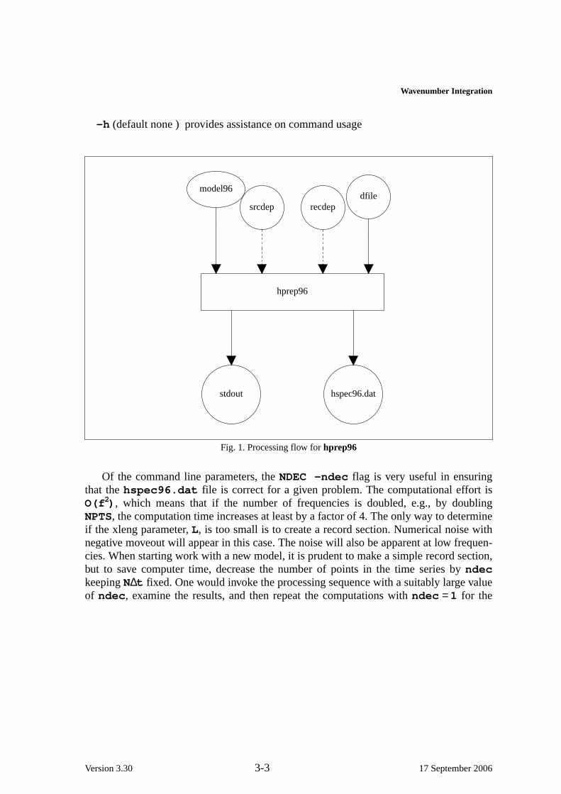
-h (default none ) provides assistance on command usage

hprep96

stdout hspec96.dat

model96

srcdep recdepdfile

Fig. 1. Processing flow for hprep96

Of the command line parameters, theNDEC -ndec flag is very useful in ensuringthat thehspec96.dat fi le is correct for a given problem. The computational effort isO(f 2) , which means that if the number of frequencies is doubled, e.g., by doublingNPTS, the computation time increases at least by a factor of 4. The only way to determineif the xleng parameter, L, is too small is to create a record section. Numerical noise withnegative moveout will appear in this case. The noise will also be apparent at low frequen-cies. When starting work with a new model, it is prudent to make a simple record section,but to sav e computer time, decrease the number of points in the time series byndeckeepingN∆t fixed. One would invoke the processing sequence with a suitably large valueof ndec , examine the results, and then repeat the computations withndec = 1 for the



final run.

3. hspec96

Figure 3 shows the processing flow for this program. The program requires thehspec96.dat fi le created byhprep96(VI). The program output is onstdout and on abinary filehspec96.grn.


hspec96 [flags], where the command flags are-H (default false) UseHankel function not Bessel. This will be useful at large dis-

tances and high frequencies, especially when phase velocity windowing is per-formed.

-A arg (default arg=3.0) value ofkr whereHn(k r) replacesJn(k r) in integration -only used when -H is used

-K (default Futterman) use Kjartansson Causal Q

The following govern wav efield at source. The default is the entire wav efield-SU (default whole wav efield) Compute only upgoing wav efield from the source-SD (default whole wav efield) Compute only downgoing wav efield from the source-SPUP Include upward P at source-SSUP Include upward S at source-SPDN Include downward P at source-SSDN Include downward S at source

The following govern the wav efield at the receiver. The default is the entire wav efield.The usefulness and effect of these for a surface receiver is not clear.

-RD Include only downgoing wav es at receiver-RU Include only upgoing wav es at receiver-RPUP Include upward P at receiver-RSUP Include upward S at receiver-RPDN Include downward P at receiver-RSDN Include downward S at receiver-?-h Online help concerning program usage



hspec96

stdout hspec96.grn

model96 hspec96.dat

Fig. 2. Processing flow for hspec96

4. hpulse96

Figure 3 shows the processing flow for this program. The program requires thehspec96.grn fi le created byhspec96(V)and optionally the source pulse definition filerfile. The program output is onstdout and is a time series infi le96(V) format.


hpulse96 [flags], where the command flags are-t Triangular pulse of base 2 L dt-p Parabolic Pulse of base4 L dt-o Ohnaka pulse with parameter alpha-i Dirac Delta function-l L Source duration factor for the parabolic and triangular pulses.-a alpha Shape parameter for Ohnaka pulse-D Output is ground displacement-V Output is ground velocity (default)-A Output is ground acceleration-F rfile User supplied pulse-m mult Multiplier (default 1.0)



-OD Output is forced to be named displacement-OV Output is forced to be named velocity-OA Output is forced to be named acceleration

-Z zero phase triangular/parabolic pulse, else causal-?-h Online help concerning program usage

hpulse96

stdoutfi le96

hspec96.grnrfile

Fig. 3. Processing flow for hpulse96

5. Sample Run




rbh> hprep96 -M model.d -d dfile -HS 10 -HR 0 -ALL

rbh> hspec96 > hspec96.out

rbh> hpulse96 -V -p -l 4 | f prof96


1 0 . 0 0 0 00 . 0 0 0 0

1 . 2 4 2 E - 0 41 0 . 0 0 0 0

1 0 . 0 0 0 00 . 0 0 0 0

1 . 0 2 9 E - 0 42 0 . 0 0 0 0

1 0 . 0 0 0 00 . 0 0 0 0

7 . 7 4 6 E - 0 53 0 . 0 0 0 0

1 0 . 0 0 0 00 . 0 0 0 0

6 . 1 8 5 E - 0 54 0 . 0 0 0 0

1 0 . 0 0 0 00 . 0 0 0 0

5 . 0 0 1 E - 0 55 0 . 0 0 0 0

1 0 . 0 0 0 00 . 0 0 0 0

4 . 1 8 4 E - 0 56 0 . 0 0 0 0

1 0 . 0 0 0 00 . 0 0 0 0

3 . 5 0 6 E - 0 57 0 . 0 0 0 0

1 0 . 0 0 0 00 . 0 0 0 0

3 . 0 8 5 E - 0 58 0 . 0 0 0 0

1 0 . 0 0 0 00 . 0 0 0 0

2 . 8 1 2 E - 0 59 0 . 0 0 0 0

1 0 . 0 0 0 00 . 0 0 0 0

2 . 4 3 3 E - 0 51 0 0 . 0 0 0 0

18 24 30 36 42

SRC = TSS D T = 0 . 1 2 5 0 0 0model .d

Fig. 4. TSS Green’s function for the layered model.

6. hwhole96

This program computes synthetics for a wholespace using the properties of the firstlayer of the model. This program has two important uses. First, a wholespace solution isfundamental in the development of seismic wav etheory. Second, this analytical solutionpermits a direct test of the wav enumber integration used byhspec96. Since an analyticalsolution is used, wav enumber integration is not performed. The excitation of this programis very rapid. Figure 5 shows the processing flow for this program. The program



requires thehspec96.dat fi le created byhprep96(VI). The program output is onstdoutand on a binary filehspec96.grn.


hwhole96 [flags], where the command flags are-K (default Futterman) use Kjartansson Causal Q-?-h


hwhole96

stdout hspec96.grn

model96 hspec96.dat

Fig. 5. Processing flow for hwhole96

rbh> hprep96 -M model.d -d dfile -HS 10 -HR 0 -ALL

rbh> hwhole96 > hspec96.out





1 0 . 0 0 0 00 . 0 0 0 0

6 . 4 8 9 E - 0 51 0 . 0 0 0 0

1 0 . 0 0 0 00 . 0 0 0 0

5 . 1 2 5 E - 0 52 0 . 0 0 0 0

1 0 . 0 0 0 00 . 0 0 0 0

3 . 8 1 8 E - 0 53 0 . 0 0 0 0

1 0 . 0 0 0 00 . 0 0 0 0

3 . 0 7 2 E - 0 54 0 . 0 0 0 0

1 0 . 0 0 0 00 . 0 0 0 0

2 . 4 9 4 E - 0 55 0 . 0 0 0 0

1 0 . 0 0 0 00 . 0 0 0 0

2 . 0 8 9 E - 0 56 0 . 0 0 0 0

1 0 . 0 0 0 00 . 0 0 0 0

1 . 7 5 2 E - 0 57 0 . 0 0 0 0

1 0 . 0 0 0 00 . 0 0 0 0

1 . 5 3 9 E - 0 58 0 . 0 0 0 0

1 0 . 0 0 0 00 . 0 0 0 0

1 . 4 0 3 E - 0 59 0 . 0 0 0 0

1 0 . 0 0 0 00 . 0 0 0 0

1 . 2 1 4 E - 0 51 0 0 . 0 0 0 0

18 24 30 36 42

SRC = TSS D T = 0 . 1 2 5 0 0 0model .d

Fig. 6. Whole space response for TSS Green’s function.

7. hspec96p

This program computes the p-τ response for a layered media. The wav enumber inte-gration method for computing synthetic seismograms consists of evaluating the doubleintegral

g(r, t) =∞

−∞∫ g(r, f)ej2π ftdf

where

g(r, f) =∞

0∫ g(k, f)Jn(kr)kdk

Since this equation is a Hankel transform, we also have

g(k, f) =∞

0∫ g(r, f)Jn(kr)rdr

In exploration seismology it convenient to think in terms of ray parameterp which is



related tok andω = 2π f by k = pω . By substitution, we can defineg(p,τ ) as

g(p,τ ) = g(p, t − pr) =∞

−∞∫ g(k = 2π fp, f )ej2π f(t−pr)df

=∞

−∞∫ g(k = 2π fp, f)ej2π fτ df

This last expression shows that thep − τ response is actually the inverse Fourier trans-form of g(k, f) with the constraint k= p2π f.

The p− τ seismogram has several interesting properties. Reflection hyperbolas in ther − t domain, appear as ellipses in thep − τ domain. A refracted arrival with ray parame-ter, prefr, is mapped into a point with ray parameterprefr in thep − τ domain. Moreimpor-tantly, the effect of the Hankel transform is that geometrical spreading is removed. Thep − τ time history gives correct relative amplitudes due to plane wav e reflection andrefraction in the model.

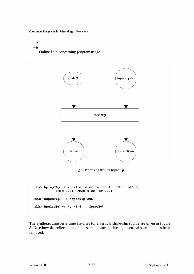
Figure 7 shows the processing flow for this program. The program requires thehspec96p.dat fi le created byhprep96p(VI). The program output is onstdout and on abinary filehspec96.grn.

Program control for the programhprep96p is through command line flags. The pro-gram is similar in concept to that ofhprep96, except for two important points. First theoutput is a file by the namehspec96p.dat. Since we are interested in p-τ time histories,distance is immaterial; ray parameter is the important parameter. The distance file, indi-cated by the command line flag-d dfile is important since this defines the sampling inter-val and the number of points in the time series. The use of the same file rather thananother one, means that one can easily obtain time histories in the r-t space and the p-τspace using the same data files, as indicated by the examples in this chapter. The programhprep96p is executed as follows:

hprep96p [flags], where the command flags are-M model (default none ) Earth model file-d dfile (default none ) Name of distance file



whereDIST is the epicentral distance in kilometers,DT is the sampling interval forthe time series,NPTSis the number of points in the time series ( a power of 2).For this program the entries DIST T0 and VRED are NOT used. They are includein the input for compatibility with the synthetic seismogram programs.

-FHS srcdep (overrides -HS ) Name of source depthfi le-FHR recdep (overrides -HR ) Name of receiver depth file-HS hs (default 0.0 ) Source depth-HR hr (default 0.0 ) Receiver depth-TF (default true ) top surface is free



-TR (default false) topsurface is rigid-TH (default false) topsurface is halfspace-BF (default false) bottomsurface is free-BR (default false) bottomsurface is rigid-BH (default true ) bottom surface is halfspace-ALL (default true ) Compute all Green s functions-EQEX (default false) Computeearthquake/explosion Green s functions-EQF (default false) Computeexplosion/point force Green s functions-PMIN pmin -PMAX pmax -DP dp (default none) ray parameter sample space

in sec/km-TRUE (default false) use modified p-tau response. For a simple direct body wav e

arrival, the pulse of the vertical and horizontal components are Hilbert transformsof each other, because has a different ordern of the Bessel functions. This programautomatically adjusts the phase of the radial components byπ /2 radians, unlessspecifically instructed not to by this command. Application of the correct order ofthe Hankel transform to observed three component data would result in the samephase difference, and this option is provided for a direct comparison.

-NDEC ndec (default 1) decimate the time series-ALP alp (default 2.5) time domain damping factor. The end of the trace is reduced

by a factor ofe−alp to reduce the effects of Discrete Fourier Transform periodicity.Note, if hspec96pis used for site spectral response, then setalpha = 0.0 . Fortime series, use the default.

-? (default none ) this help message-h (default none ) this help message

Program control forhspec96pis through the command line:

hspec96p [flags], where the command flags are-K (default Futterman) use Kjartansson Causal QThe following govern wav efield at source. The default is the entire wav efield-SU (default whole wav efield) Compute only upgoing wav efield from the source-SD (default whole wav efield) Compute only downgoing wav efield from the source-SPUP

Include upward P at source-SSUP

Include upward S at source-SPDN

Include downward P at source-SSDN

Include downward S at sourceThe following govern wav efield at receiver. The default is the entire wav efield-RD Include only downgoing wav es at receiver-RU Include only upgoing wav es at receiver-RPUP Include upward P at receiver-RSUP Include upward S at receiver-RPDN Include downward P at receiver-RSDN Include downward S at receiver



-?-h


hspec96p

stdout hspec96.grn

model96 hspec96p.dat

Fig. 7. Processing flow for hspec96p

rbh> hprep96p -M model.d -d dfile -HS 10 -HR 0 -ALL \-PMIN 0.01 -PMAX 0.20 -DP 0.01

rbh> hspec96p > hspec96p.out


The synthetic transverse time histories for a vertical strike-slip source are given in Figure8. Note how the reflected amplitudes are enhanced, since geometrical spreading has beenremoved.



1 0 . 0 0 0 00 . 0 0 0 0

1 . 6 2 4 E - 0 40 . 0 1 0 0

1 0 . 0 0 0 00 . 0 0 0 0

3 . 2 5 2 E - 0 40 . 0 2 0 0

1 0 . 0 0 0 00 . 0 0 0 0

4 . 8 8 9 E - 0 40 . 0 3 0 0

1 0 . 0 0 0 00 . 0 0 0 0

6 . 5 3 5 E - 0 40 . 0 4 0 0

1 0 . 0 0 0 00 . 0 0 0 0

8 . 1 8 7 E - 0 40 . 0 5 0 0

1 0 . 0 0 0 00 . 0 0 0 0

9 . 9 2 7 E - 0 40 . 0 6 0 0

1 0 . 0 0 0 00 . 0 0 0 0

1 . 1 7 2 E - 0 30 . 0 7 0 0

1 0 . 0 0 0 00 . 0 0 0 0

1 . 3 5 3 E - 0 30 . 0 8 0 0

1 0 . 0 0 0 00 . 0 0 0 0

1 . 5 3 6 E - 0 30 . 0 9 0 0

1 0 . 0 0 0 00 . 0 0 0 0

1 . 7 2 4 E - 0 30 . 1 0 0 0

1 0 . 0 0 0 00 . 0 0 0 0

1 . 9 3 5 E - 0 30 . 1 1 0 0

1 0 . 0 0 0 00 . 0 0 0 0

2 . 1 4 3 E - 0 30 . 1 2 0 0

1 0 . 0 0 0 00 . 0 0 0 0

2 . 3 6 1 E - 0 30 . 1 3 0 0

1 0 . 0 0 0 00 . 0 0 0 0

2 . 6 0 8 E - 0 30 . 1 4 0 0

1 0 . 0 0 0 00 . 0 0 0 0

2 . 8 4 3 E - 0 30 . 1 5 0 0

1 0 . 0 0 0 00 . 0 0 0 0

3 . 1 3 6 E - 0 30 . 1 6 0 0

1 0 . 0 0 0 00 . 0 0 0 0

3 . 4 2 2 E - 0 30 . 1 7 0 0

1 0 . 0 0 0 00 . 0 0 0 0

3 . 7 5 7 E - 0 30 . 1 8 0 0

1 0 . 0 0 0 00 . 0 0 0 0

4 . 1 3 1 E - 0 30 . 1 9 0 0

1 0 . 0 0 0 00 . 0 0 0 0

4 . 5 3 4 E - 0 30 . 2 0 0 0

0 6 12 18 24

SRC = TSS D T = 0 . 1 2 5 0 0 0model .d

Fig. 8. The p-τ response for the TSS Green’s function. Theannotation at the right indi-cated the maximum trace amplitude, the fact that the source depth was 10.0 km, the rayparameter, and the receiver depth.



CHAPTER 4MODAL SUMMATION

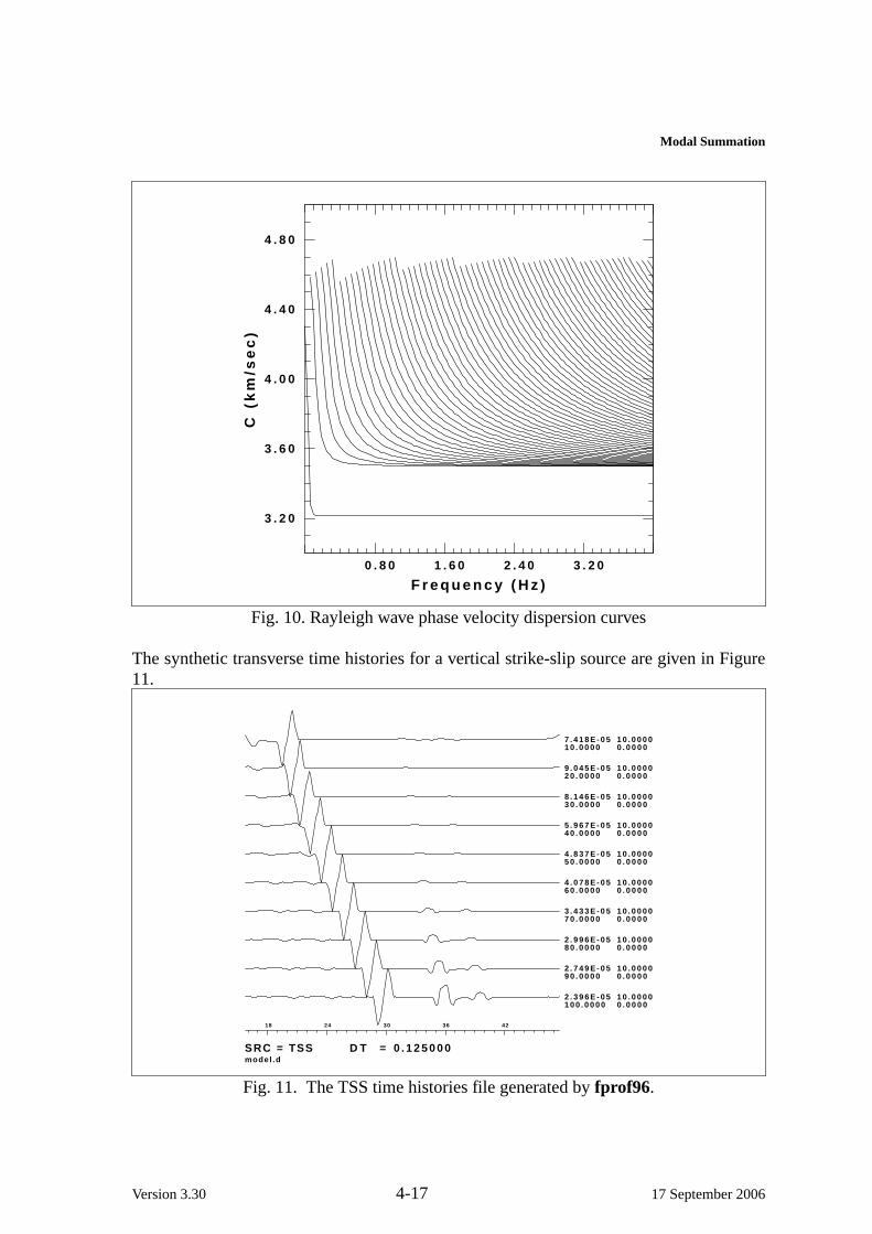
1. Introduction model96

sprep96

sdisp96

scomb96

slegn96sregn96

spulse96

fi le96

sdpsrf96

sdpegn96sdpder96

This chapter describes the use ofmodal superposition of surface wav es tocreate synthetic seismograms.For lowfrequency seismograms, this techniquecan be much faster than wav enumberintegration and generalized ray tech-niques. In addition, extension of themodel by adding a high velocity cap zoneat great depth permits the computation ofalmost complete synthetic seismogramsby the locked mode approximation.There are four stages between the specifi-cation of the model file and the final syn-thetic seismograms.

The programsprep96creates a data file sdisp96.dat for use bysdisp96to determinethe multimode phase velocity dispersion for the model.slegn96and sregn96computethe eigenfunctions required for synthetics from the dispersion curves. Finally, spulse96uses the eigenfunction and dispersion information to create the required Green’s func-tions infi le96 format. The programscomb96can be used to correct the dispersion curvesgenerated bysdisp96by filling in missing modes. The programssdpsrf96andsdpegn96are used to display the dispersion curves and thus provide a quality control check.Theprogramsdpder96 lists and plots the depth dependence of surface-wav eeigenfunctionsand phase velocity partial derivatives.

Given the capabilities of modern computers, it is possible to combine all these func-tions into a single large program, but the modularapproach used permits intervention forquality control at each stage, since determination of dispersion curves is not trivial.

2. sprep96



Figure 1 shows the processing flow for this program.The program requires an earthmodel file in themodel96 format and two optional control files. The output consists ofthe filesdisp96.dat.

sprep96

stdout sdisp96.dat

model96period

fi lefrequency

fi le

Fig. 1. Processing flow for sprep96


sprep96 [flags], where the command flags are-M model (default none ) Earth model file-d dfile (default none ) Name of distance file



whereDIST is the epicentral distance in kilometers,DT is the sampling interval forthe time series,NPTSis the number of points in the time series ( a power of 2).T0and VREDare used to define the time of the first sample point which isT0 +DIST/VRED if VRED ≠ 0 or T0 if VRED = 0 .This program only uses the DT and NPTS entries to define the frequency range ofdesired dispersion


Modal Summation

-HS hs (default 0.0 ) Source depth-HR hr (default 0.0 ) Receiver depth-DT dt (default 1.0 ) Sampling interval-NPTS npts (default 1 ) Number of points-NMOD nmodes (default 1 ) Maximum number of modes-L (default false) Generate Love Wav es-R (default false) Generate Rayleigh Wav es

Note that at least one of these must be specified. Also note that Love waves do notexist in a halfspace.

-FACL faclov (default 5.0) parameter for controlling root search. A small numberis faster, but higher modes may be missed.

-FACR facray (default 5.0) parameter for controlling root search-FREQ freq User specified single frequency. This permits dispersion computation

for a single frequency. This cannot be used for synthetics.-PER period User specified single period. This permits dispersion computation

for a single period. This cannot be used for synthetics.-FARR freq_file User specified file of separate frequencies on each line. This

permits dispersion computation for a list of specified frequencies.This cannot beused for synthetics.

-PARR period_file File of user specified periods User specified file ofseparate periods on each line. This permits dispersion computation for a list ofspecified periods.This cannot be used for synthetics.

NOTE: one of -DT -NPTS, -FARR, -PARR, -PER or -FREQ required-?-h (default none ) this help message

3. sdisp96

This program computes the dispersion curves for the given earth model. This pro-gram calculates the desired dispersion curves for the model. All program control isthrough the file sdisp96.dat created by the programsprep96. The output consists the ofbinary dispersion files for Love and Rayleigh wav es: sdisp96.lov andsdisp96.ray, respec-tively.


sdisp96 [flags], where the command flags are-v (default none ) On a PC, the frequency of each computation is written to the

screen on the same line to indicate that the program is actually working. Thiscan-not be easily done with UNIX since UNIX does not support the formatting parame-ter ’+’, but instead scrolls the screen..

-?-h (default none ) this help message



Figure 2 shows the processing flow for this program.

sdisp96

stdout sdisp96.lovsdisp96.ray

model96 sdisp96.dat

Fig. 2. Processing flow for sdisp96

4. scomb96

This program redoes the root determination ofsdisp96 in a user defined rectangularregion. Thismay be necessary if modes are missed.Missing modes are seen by visualinspection of the dispersion curves usingsdpsrf96. This program calculates the desireddispersion curves for the model. All program control is through the file sdisp96.dat andthe command line.For Love wav es, the input is the file sdisp96.lov and the output is thebinary dispersion file tsdisp96.lov. For Rayleigh wav es, the input is the file sdisp96.rayand the output is the binary dispersion filetsdisp96.ray.

the difference in the input and output file names is to preserve the original file. Ifmany sequential repairs must be made, the user must systematically renametsdisp96.lovto sdisp96.lov for Love wav es and similarly for the Rayleigh wav es.


scombf96 [flags], where the command line flags are


Modal Summation

-L Recompute the Love wav edispersion contained in the filesdisp96.lov.-R Recompute the Rayleigh wav edispersion contained in the file sdisp96.ray. br Note

that either -L or -R must be specified-TMIN Minimum value of period for search region-TMAX Maximum value of period for search region-FMIN Minimum value of frequency for search region-FMAX Maximum value of frequency for search region-CMIN Minimum value of phase velocity for search region-CMAXMaximum value of phase velocity for search region-FAC factor Factor to control density of search-I Ignore existing zeros within [CMIN, CMAX] and restart the search-?-h On line command help On line command help

Figure 3 shows the processing flow for this program.

scomb96

stdouttsdisp96.lovtsdisp96.ray

model96sdisp96.lovsdisp96.ray

Fig. 3. Processing flow for scomb96

5. slegn96/sregn96



Figure 4 shows the processing flow for these programs.The programslegn96requires thesdisp96.lov fi le created bysdisp96 (or the tsdisp96.lov fi le created byscomb96) and the programsregn96requires thesdisp96.ray fi le created bysdisp96(orthe tsdisp96.lov fi le created byscomb96). Thecommon purpose of these programs is tocompute the eigenfunctions corresponding to the dispersion curves for Love and Rayleighwaves, respectively. The eigenfunctions so created for use by the synthetic seismogramprogramspulse96are stored in the filesslegn96.egn andsregn96.egn, respectively.

Program control is through the command line and is identical for each program:

slegn96 [flags], where the command line flags are-FHS srcdepth_file (overrides -HS ) Name of source depthfi le-FHR recdepth_file (overrides -HR ) Name of receiver depth file-HS src_depth Source depth, overrides previously given value-HR rec_depth Receiver depth, overrides previously given value-NOQIgnore the Q model. Compute purely elastic dispersion-T Use the dispersion filetsdisp96.lov instead ofsdisp96.lov.-DER output all depth dependent values (default false)-DE output eigenfunctions(depth) (default false)-DH output DC/DH(depth) (default false)-DB output DC/DB(depth) (default false)-DR output DC/DR(depth)-?-h Write this help message (default false)

sregn96 [flags], where the command line flags are-FHS srcdepth_file (overrides -HS ) Name of source depthfi le-FHR recdepth_file (overrides -HR ) Name of receiver depth file-HS src_depth Source depth, overrides previously given value-HR rec_depth Receiver depth, overrides previously given value-T Use the dispersion filetsdisp96.ray instead ofsdisp96.ray.-DER output all depth dependent values (default false)-DE output eigenfunctions(depth) (default false)-DH output DC/DH(depth) (default false)-DA output DC/DA(depth). This only applies to the programsregn96 since Love

waves are independent of P-wav evelocity. (default false)-DB output DC/DB(depth) (default false)-DR output DC/DR(depth)-?-h Write this help message

Note that if the flags -DER, -DH, -DA , -DB or -DR are set, only the file slegn96.derorsregn96.der is computed. If these flags are not set, then only the file sregn96.egnorslegn96.egnare created. The files slegn96.derand sregn96.derare created for use inwaveform inversion or other programs.


Modal Summation

slegn96

slegn96.egnslegn96.der

sdisp96.lovtsdisp96.lov

sregn96

sregn96.egnsregn96.der

sdisp96.raytsdisp96.ray

Fig. 4. Processing flow for slegn96andsregn96

6. spulse96

Figure 5 shows the processing flow for this program. The program requires either orboth of the files slegn96.egn sregn96.egn to compute synthetic seismograms on the stan-dard output infi le96format.

Program control is through the command line:spulse96 [flags], where the command line flags are

-d Distance_File Distance control fileThe required distance file. The file contains the following ASCII entries per line:



-v Verbose output-t Triangular pulse of base 2 L dt-p Parabolic Pulse of base4 L dt-l L Duration control parameter for triangular and parabolic pulses-o Ohnaka pulse with parameter alpha-i Dirac Delta function-a alpha Shape parameter for Ohnaka pulse-D Output is ground displacement



-V Output is ground velocity (default)-A Output is ground acceleration-F rfile User supplied pulse-m mult Multiplier (default 1.0)-OD Output is forced to be named displacement-OV Output is forced to be named velocity-OA Output is forced to be named acceleration-EX Explosion and point force green s functions-EQ Earthquake and double couple green s functions-ALL Earthquake, Explosion and Point Force-LAT (default false) Laterally varying eigenfunctions produced by slat96-2 (default false) Use double length FFT internally (alleviates FFT wrap around)-M [ nmode ] (default all) mode number to compute. [0=fund,1=1st]-FUND (default all) use fundamental modes only for the synthetic-HIGH (default all) use all higher modes only for the synthetic-LOCK locked mode used. This does not affect the synthetics, but drops the artificial,

high velocity bottom layer from the first arrival time computation. There is no wayto define this from the earth model.

-Z zero phase triangular/parabolic pulse, else causal-?-h Write this help message

7. sdpsrf96

This programs reads the phase velocity dispersion file created bysdisp96and plotsthe dispersion curves. A listing is optional.The output isa CALPLOT file with nameSDISPL.PLT or SDISPR.PLT for Love and Rayleigh wav edispersion, respectively. If the-TXT flag is used, then a listing of the dispersion information is on file SDISPL.TXT orSDISPR.TXT for Love and Rayleigh wav es, respectively. Figure 6 shows the processingflow for this program.

Program control is through the command line:sdpsrf96 [flags], where the command line flags are

-L Plot the Love wav edispersion contained in the filesdisp96.lov.-R Plot the Rayleigh wav edispersion contained in the file sdisp96.ray. br Note that

either -L or -R must be specified, but not both.-FREQ the X-axis is frequency (default)-PER the X-axis is period-XMIN Minimum value of X-axis-XMAXMaximum value of X-axis(default is automatic determination of limits)-YMIN Minimum value of phase velocity for vertical axis-YMAXMaximum value of phase velocity for vertical axis-X0 x0 (default 2.0 in = 5.08 cm)-Y0 y0 Absolute coordinates of lower left corner of plot (default 1.0 in = 2.54 cm)


Modal Summation

spulse96

stdoutfi le96

slegn96.egn sregn96.egn dfile rfile

Fig. 5. Processing flow for spulse96

-XLEN xlen Length of X-axis (default 6.0 in = 15.24 cm)-YLEN ylen (default 6.0) Length of Y-axis-K kolor CALPLOT color code for dispersion curves. Default=1-NOBOXDo not plot the coordinate axes, only plot corner tics. This is useful for over-

laying several plots.-TXT (default .false.) create a text file listing of the dispersion with the name

SDISPL.TXT or SDISPR.TXT for Love and Rayleigh wav es, respectively.-ASC (default .false.) create an ASCII text file listing of the dispersion with the name

SDISPL.ASC or SDISPR.ASC for Love and Rayleigh wav es, respectively. Thesefi les have a single single line header followed by numeric column entries as in thissmall exerpt for a

sdpsrf96 -L -ASC

LMODE NFREQ PERIOD(S) FREQUENCY(Hz) C(KM/S)0 1 2.000000000 0.5000000000 3.5534143310 2 2.000977040 0.4997558594 3.5534176310 3 2.001955034 0.4995117188 3.553420936

Here the columns are mode (with 0 for fundamental), the unique frequency num-ber, the period, frequency and phase velocity.

-T Use the dispersion files tsdisp96.lov or tdisp96.ray instead of sdisp96.lov orsdisp96.ray, respectively.

-XLOGX-axis is logarithmic (default is false)-?



-h On line command help

sdpsrf96

SDISPL.PLTSDISPL.TXTSDISPL.ASC

SDISPR.PLTSDISPR.TXTSDISPR.ASC

sdisp96.lovtsdisp96.lov sdisp96.ray

tsdisp96.ray

Fig. 6. Processing flow for sdpsrf96

8. sdpegn96

This programs reads the eigenfunction file created byslegn96or sregn96and plotsthe curves. A listing is also permitted. The output isa CALPLOT file with nameSLEGNU.PLT or SREGNU.PLT for Love and Rayleigh wav egroup-velocity dispersion,respectively, SLEGNC.PLT or SREGNC.PLT for Love and Rayleigh wav ephase-velocitydispersion, respectively, and SLEGNG.PLT or SREGNG.PLT for Love and Rayleighanelastic attenuation coefficient, respectively. Figure 7 shows the processing flow for thisprogram. Inthe presence of Q, the phase velocities will be those for causal Q, but thegroup velocities are only for infinite Q.

Program control is through the command line:sdpegn96 [flags], where the command line flags are

-L Plot the Love wav edispersion contained in the filesdisp96.lov.-R Plot the Rayleigh wav edispersion contained in the filesdisp96.ray.

Note that either -L or -R must be specified


Modal Summation

-U Plot the group velocity dispersion-C Plot the phase velocity dispersion-G Plot the anelastic attenuation coefficient

Note that either -U , -C or -G must be specified-FREQ the X-axis is frequency (default)-PER the X-axis is period-XMIN Maximum value of X-axis-XMAXMinimum value of X-axis-YMIN Minimum value of phase velocity for vertical axis-YMAXMaximum value of phase velocity for vertical axis-X0 x0 (default 2.0)-Y0 y0 Absolute coordinates of lower left corner of plot (default 1.0)-XLEN xlen Length of X-axis (default 6.0)-YLEN ylen Length of Y-axis (default 6.0)-K kolor CALPLOT color code for dispersion curves. Default=1-NOBOXDo not plot the coordinate axes, only plot corner tics. This is useful for over-

laying several plots.-TXT (default .false.) create a text file listing of the dispersion in files names

SDISPL.TXT or SDISPR.TXT for Love and Rayleigh wav es respectively.-ASC (default .false.) create an ASCII text file listing of the dispersion in files names

SDISPL.ASC or SDISPR.ASC for Love and Rayleigh wav es respectively. Thesefi les have a single single line header followed by numeric column entries as in thissmall exerpt for a

sdpegn96 -R -ASC

RMODE NFREQ PERIOD(S) FREQUENCY(Hz) C(KM/S) U(KM/S) ENERGY GAMMA(1/KM) ELLIPTICITY

0 1 2.0000 0.50000 3.2632 3.2640 0.14010E-01 0.48125E-03 0.68118

0 2 2.0010 0.49976 3.2632 3.2640 0.14003E-01 0.48102E-03 0.68118

0 3 2.0020 0.49951 3.2632 3.2640 0.13996E-01 0.48078E-03 0.68118

0 4 2.0029 0.49927 3.2632 3.2640 0.13989E-01 0.48055E-03 0.68118

0 5 2.0039 0.49902 3.2632 3.2640 0.13982E-01 0.48031E-03 0.68118

Here the columns are mode (with 0 for fundamental), the unique frequency num-ber, the period, frequency, phase velocity, group velocity, energy integral, anelasticattenuation coefficient (exp( −gammdistance) , and for Rayleigh wav es, theellipticity..

-XLOG (default linear) X axis is logarithmic-D dispfile (default ignore) plot dispersion values from the file dispfile which is in

SURF96 dispersion format. Only those values specified by the-L , -R , -U , -C and-G specific flag combination are plotted. The purpose is to plot observed disper-sion on top of model predicted dispersion.

-DE dispfile (default ignore) plot dispersion values from the file dispfile which is inSURF96 dispersion format. Only those values specified by the-L , -R , -U , -C and-G specific flag combination are plotted. The purpose is to plot observed disper-sion and error bars on top of model predicted dispersion.

-S (default no) create output theoretical dispersion values in files in SURF96 format.All values, group velocity, phase velocity and gamma wil be placed into a filenamedSLEGN.dsp or SREGN.dsp. Artif icial low values will be placed in the error



field.-?-h On line command help

sdpegn96

SLEGNC.PLTSLEGNU.PLTSLEGNG.PLT

SLEGN.TXTSLEGN.ASCSLEGN.dsp

SREGNC.PLTSREGNU.PLTSREGNG.PLT

SREGN.TXTSREGN.ASCSREGN.dsp

slegn96.egn sregn96.egn

Fig. 7. Processing flow for sdpegn96

9. sdpder96

This programs reads the depth dependent eigenfunction file created by the-DER,-DH, -DA, -DB or -DR options ofslegn96or sregn96and plots the curves. A listing isalso permitted. The output isa CALPLOT file with nameSLDER.PLT or SRDER.PLTand optionally the ASCII files SLRDER.TXT and SRDER.TXT, for Love and Rayleighwave functions, respectively. Figure 8 shows the processing flow for this program.

Program control is through the command line:sdpder96 [flags], where the command line flags are

-L Plot the Love wav edepth dependent functions contained in the fileslegn.der.-R Plot the Rayleigh wav edepth dependent functions contained in the filesregn.der.

Note that either -L or -R must be specified-XMAXMaximum value of X-axis-XMIN Minimum value of X-axis-YMIN Minimum value of independent variable-YMAXMaximum value of independent variable


Modal Summation

-X0 x0 (default 2.0)-Y0 y0 Absolute coordinates of lower left corner of plot (default 1.0)-XLEN xlen Length of X-axis (default 6.0)-YLEN ylen Length of Y-axis (default 6.0)-K kolor CALPLOT color code for dispersion curves. Default=1-NOBOXDo not plot the coordinate axes, only plot corner tics. This is useful for over-

laying several plots.-CLEAN (default false) No period,mode annotation on the plot-TXT (default .false.) create a text file listing of the dispersion-?-h On line command help

sdpder96

SLDER.PLT SLDER.TXT SRDER.PLT SRDER.TXT

slegn96.der sregn96.der

Fig. 8. Processing flow for sdpder96

10. sdpdsp96

This programs readsSURF96 dispersion files and plots them on axes in the same manneras sdpder96. The purpose of the program is to compare observations with predictions.The output isa CALPLOT file with nameSLDSPU.PLT or SRDSPU.PLT for Love andRayleigh wav egroup-velocity dispersion, respectively, SLDSPC.PLT or SRDSPC.PLT forLove and Rayleigh wav e phase-velocity dispersion, respectively, and SLDSPG.PLT orSRDSPG.PLT for Love and Rayleigh anelastic attenuation coefficient, respectively. Up to100 files can be plotted, but this is certainly beyond the capabilities of command lineinput.



Program control is through the command line:sdpdsp96 [flags], where the command line flags are

-L Plot the Love wav edispersion contained in the filesdisp96.lov.-R Plot the Rayleigh wav edispersion contained in the filesdisp96.ray.

Note that either -L or -R must be specified-U Plot the group velocity dispersion-C Plot the phase velocity dispersion-G Plot the anelastic attenuation coefficient

Note that either -U , -C or -G must be specified-FREQ the X-axis is frequency (default)-PER the X-axis is period-XMIN Maximum value of X-axis-XMAXMinimum value of X-axis-YMIN Minimum value of phase velocity for vertical axis-YMAXMaximum value of phase velocity for vertical axis-X0 x0 (default 2.0)-Y0 y0 Absolute coordinates of lower left corner of plot (default 1.0)-XLEN xlen Length of X-axis (default 6.0)-YLEN ylen Length of Y-axis (default 6.0)-S symsiz (default 0.03) size of observed symbol.-K kolor CALPLOT color code for dispersion curves. Default=1-NOBOXDo not plot the coordinate axes, only plot corner tics. This is useful for over-

laying several plots.-XLOG (default linear) X axis is logarithmic-D dispfile (default ignore) plot dispersion values from the file dispfile which is in

SURF96 dispersion format. Only those values specified by the-L , -R , -U , -C and-G specific flag combination is plotted. The purpose is to plot observed dispersionon top of model predicted dispersion. The dispersion values have a size specifiedby the size parameter below, and a symbol shape keyed on the mode number.

-DE dispfile (default ignore) plot dispersion values from the file dispfile which is inSURF96 dispersion format. Only those values specified by the-L , -R , -U , -C and-G specific flag combination is plotted. The purpose is to plot observed dispersionand error bars on top of model predicted dispersion.The dispersion values have asize specified by the size parameter below, and a symbol shape keyed on the modenumber.

-DC dispfile (default ignore) plot dispersion values from the file dispfile which is inSURF96 dispersion format as acontinueous curve. Only those values specified bythe -L , -R , -U , -C and -G specific flag combination is plotted.Typically this filewill be obtained fromsdpegn96.

-?-h On line command help

11. sdprad96

This program plots theoretical radiation pattern plots for a given period, mode and wav etype. This program is used as a final step in determining focal mechanisms from surface


Modal Summation

wave spectral amplitude radiation patterns.

To use this program it is necessary to run the programssregn96 -DER andslegn96 -DER to generate the binary files, sregn96.der andslegn96.der, of eigenfunc-tions as a function of depth.

The output of the program is a either aSRADR.PLT or aSRADL.PLT CALPLOTfi le.The plot consists of the radiation pattern with a maximum radius of 1 inch (2.54 cm), thetheoretical radiation pattern in black, the observed data points in red, a scale indicatingthe spectral amplitude in units ofcm-sec, and the observation period. The command linerequired a target distance,dist. Observed data at a distance,r are first corrected foranelastic attenuation by using the model derived γ by multiplication by the factorexp(+γ r) and then propagated to the reference distance my multiplication by the factor√ r/dist.

If the observed data file is not available, just the theoretical radiation pattern is plot-ted.

Program control is through the command line:sdprad96 [flags], where the command line flags are

-DIP dip dip of fault plane-STK Strike strike of fault plane-RAKE Rake slip angle on fault plane-M0 Moment (def=1.0) Seismic moment in units of dyne-cm-MWmw Moment magnitude-E Explosion-fx FX -fy Fy -fZ fz

Point force amplitudes (N,E,down) in units of dynes-XX Mxx -YY Myy -ZZ Mzz -XY Mxy -XZ Mxz -YZ Myz

Moment tensor elements in units of dyne-cm-DIST dist Distancein km-HS hs Source depth in km-X0 x0 (default=1.5 ) x-coordinate of center of plot-Y0 y0 (default=1.75) y-coordinate of center of plot-O observed_data File with observations in MFT96 format-PER period (default 20.0 sec) desired period-M mode (default 0)desired mode (0-Fund)-L (default Rayl)Plot Love wav eradiation-R (default Rayl)Plot Rayleigh wav eradiation-DMIN dmin (default 0 km ) minimum for distance sieve-DMAXdmax (default 100000 km) maximum for distance sieve-?-h On line command help

12. Sample Runs




rbh> sprep96 -HR 0 -HS 10 -M model.d -d dfile -NMOD 100 -L -Rrbh> sdisp96 > sdisp96.outrbh> sdpsrf96 -L -XMIN 0 -XMAX 4 -YMIN 3.0 -YMAX 5.0rbh> sdpsrf96 -R -XMIN 0 -XMAX 4 -YMIN 3.0 -YMAX 5.0rbh> slegn96 > s legn96.outrbh> sregn96 > sregn96.outrbh> spulse96 -d dfile -V -p -l 4 | f prof96

The phase velocity dispersion curves computed usingsdisp96and plotted usingsdpsrf96are shown in Figure 9 for Love and in Figure 10 for Rayleigh wav es.

3 . 2 0

3 . 6 0

4 . 0 0

4 . 4 0

4 . 8 0

C (

km

/se

c)

0 . 8 0 1 . 6 0 2 . 4 0 3 . 2 0

F r e q u e n c y ( H z )

Fig. 9. Love wav ephase velocity dispersion curves


Modal Summation

3 . 2 0

3 . 6 0

4 . 0 0

4 . 4 0

4 . 8 0C

(k

m/s

ec

)

0 . 8 0 1 . 6 0 2 . 4 0 3 . 2 0


Fig. 10. Rayleigh wav ephase velocity dispersion curves


1 0 . 0 0 0 00 . 0 0 0 0

7 . 4 1 8 E - 0 51 0 . 0 0 0 0

1 0 . 0 0 0 00 . 0 0 0 0

9 . 0 4 5 E - 0 52 0 . 0 0 0 0

1 0 . 0 0 0 00 . 0 0 0 0

8 . 1 4 6 E - 0 53 0 . 0 0 0 0

1 0 . 0 0 0 00 . 0 0 0 0

5 . 9 6 7 E - 0 54 0 . 0 0 0 0

1 0 . 0 0 0 00 . 0 0 0 0

4 . 8 3 7 E - 0 55 0 . 0 0 0 0

1 0 . 0 0 0 00 . 0 0 0 0

4 . 0 7 8 E - 0 56 0 . 0 0 0 0

1 0 . 0 0 0 00 . 0 0 0 0

3 . 4 3 3 E - 0 57 0 . 0 0 0 0

1 0 . 0 0 0 00 . 0 0 0 0

2 . 9 9 6 E - 0 58 0 . 0 0 0 0

1 0 . 0 0 0 00 . 0 0 0 0

2 . 7 4 9 E - 0 59 0 . 0 0 0 0

1 0 . 0 0 0 00 . 0 0 0 0

2 . 3 9 6 E - 0 51 0 0 . 0 0 0 0

18 24 30 36 42

SRC = TSS D T = 0 . 1 2 5 0 0 0model .d




The other example shows the use ofsregn96to generate depth dependent eigenfunc-tions and partial derivatives for the given model, which are displayed usingsdpder96.The following test modelmodel.wat is used.

MODELWATER MODELISOTROPICKGSFLAT EARTH1-DCONSTANT VELOCITYLINE08LINE09LINE10LINE11HR VP VS RHO QP QS ETAP ETAS FREFP FREFS

0.5 1.8 0.0 1.0 0.0 0.0 0.0 0.0 1.0 1.00.5 1.8 0.0 1.0 0.0 0.0 0.0 0.0 1.0 1.00.5 1.8 0.0 1.0 0.0 0.0 0.0 0.0 1.0 1.00.5 1.8 0.0 1.0 0.0 0.0 0.0 0.0 1.0 1.00.5 1.8 0.0 1.0 0.0 0.0 0.0 0.0 1.0 1.00.5 1.8 0.0 1.0 0.0 0.0 0.0 0.0 1.0 1.00.5 1.8 0.0 1.0 0.0 0.0 0.0 0.0 1.0 1.00.5 1.8 0.0 1.0 0.0 0.0 0.0 0.0 1.0 1.00.5 1.8 0.0 1.0 0.0 0.0 0.0 0.0 1.0 1.00.5 1.8 0.0 1.0 0.0 0.0 0.0 0.0 1.0 1.00.5 6.0 3.5 2.8 0.0 0.0 0.0 0.0 1.0 1.00.5 6.0 3.5 2.8 0.0 0.0 0.0 0.0 1.0 1.00.5 6.0 3.5 2.8 0.0 0.0 0.0 0.0 1.0 1.00.5 6.0 3.5 2.8 0.0 0.0 0.0 0.0 1.0 1.00.5 6.0 3.5 2.8 0.0 0.0 0.0 0.0 1.0 1.00.5 6.0 3.5 2.8 0.0 0.0 0.0 0.0 1.0 1.00.5 6.0 3.5 2.8 0.0 0.0 0.0 0.0 1.0 1.00.5 6.0 3.5 2.8 0.0 0.0 0.0 0.0 1.0 1.00.5 6.0 3.5 2.8 0.0 0.0 0.0 0.0 1.0 1.00.5 6.0 3.5 2.8 0.0 0.0 0.0 0.0 1.0 1.01. 8.0 4.7 3.3 0.0 0.0 0.0 0.0 1.0 1.01. 8.0 4.7 3.3 0.0 0.0 0.0 0.0 1.0 1.01. 8.0 4.7 3.3 0.0 0.0 0.0 0.0 1.0 1.01. 8.0 4.7 3.3 0.0 0.0 0.0 0.0 1.0 1.01. 8.0 4.7 3.3 0.0 0.0 0.0 0.0 1.0 1.01. 8.0 4.7 3.3 0.0 0.0 0.0 0.0 1.0 1.01. 8.0 4.7 3.3 0.0 0.0 0.0 0.0 1.0 1.01. 8.0 4.7 3.3 0.0 0.0 0.0 0.0 1.0 1.01. 8.0 4.7 3.3 0.0 0.0 0.0 0.0 1.0 1.01. 8.0 4.7 3.3 0.0 0.0 0.0 0.0 1.0 1.0

the following sequence of commands is run:


Modal Summation

rbh> sprep96 -M nmodel.wat -DT 5.0 -NPTS 2 -L -R -NMOD 2rbh> sdisp96 -vrbh> sregn96 -HS 10 -HR 20 -DER -NOQrbh> sdpder96 -R -TXT -K 2 -XLEN 3.0 -X0 1.0 -YLEN 4.0

rbh> reframe -N1 -O < SRDER.PLT > UR.PLTrbh> reframe -N2 -O < SRDER.PLT > UZ.PLTrbh> reframe -N3 -O < SRDER.PLT > TZ.PLTrbh> reframe -N4 -O < SRDER.PLT > TR.PLTrbh> reframe -N5 -O < SRDER.PLT > DH.PLTrbh> reframe -N6 -O < SRDER.PLT > DA.PLTrbh> reframe -N7 -O < SRDER.PLT > DB.PLTrbh> reframe -N8 -O < SRDER.PLT > DR.PLT

rbh> reframe -O -Y0+5000 -X0+500 < UZ.PLT > junkrbh> reframe -O -Y0+5000 -X0+5000 < UR.PLT >> junkrbh> reframe -O -Y0+5000 -X0+9500 < TZ.PLT >> junkrbh> reframe -O -Y0+5000 -X0+14000 < TR.PLT >> junkrbh> reframe -O -X0+500 < DH.PLT >> junkrbh> reframe -O -X0+5000 < DA.PLT >> junkrbh> reframe -O -X0+9500 < DB.PLT >> junkrbh> reframe -O -X0+14000 < DR.PLT >> junkrbh> mv junk ALL.PLT

In this sequence, the-DER flag to sregn96indicates that the depth dependent quantitiesshould be output at each of the initial layer boundaries. The sequence ofreframe com-mands are used to extract and reposition each of the depth plots.Figure 12 displays thesefunctions. TheDC/DH is the partial derivative of the phase velocity with respect to achange in layer thickness.

DE

PT

H

- 0 . 9 0 0 . 9 0UZ

T0=1 . 0 0 0 E + 0 1 MODE=0 C =3 . 0 0 6 E + 0 0

DE

PT

H

- 0 . 6 0 0 . 6 0UR

T0=1 . 0 0 0 E + 0 1 MODE=0 C =3 . 0 0 6 E + 0 0

DE

PT

H

- 0 . 9 0 0 . 9 0TR

T0=1 . 0 0 0 E + 0 1 MODE=0 C =3 . 0 0 6 E + 0 0

DE

PT

H

- 2 . 0 0 0 . 0 0 2 . 0 0TZ

T0=1 . 0 0 0 E + 0 1 MODE=0 C =3 . 0 0 6 E + 0 0

DE

PT

H

- 0 . 6 0 0 . 0 0 0 . 6 0DC/DH

T0=1 . 0 0 0 E + 0 1 MODE=0 C =3 . 0 0 6 E + 0 0

DE

PT

H

- 0 . 3 0 0 . 3 0DC/DA

T0=1 . 0 0 0 E + 0 1 MODE=0 C =3 . 0 0 6 E + 0 0

DE

PT

H

- 0 . 0 2 0 0 . 0 2 0DC/DB

T0=1 . 0 0 0 E + 0 1 MODE=0 C =3 . 0 0 6 E + 0 0

DE

PT

H

- 0 . 3 0 0 . 0 0 0 . 2 0 0 . 4 0DC/DR

T0=1 . 0 0 0 E + 0 1 MODE=0 C =3 . 0 0 6 E + 0 0

Fig. 12. Display of depth dependent eigenfunctions and phase velocity partial derivatives.

The next example shows how to inv oke the programsdpdsp96 to plot dispersioncurves. The files SREGN.dsp, mmsurf96.d andmsurf96.d were created by other programs.



The theoretical dispersionSREGN.dsp is plotted as a continuous curve (note that the fol-lowing command is on one line).

rbh> sdpdsp96 -R -C -PER -XLOG -YMIN 2.5 -YMAX 5 -DC SREGN.dsp-DE mmsurf96.d -DE msurf96.d -XMIN 4 -XMAX 500 -K 1025 -S 0.07

3 . 0 0

3 . 5 0

4 . 0 0

4 . 5 0

5 . 0 0

C (

km

/se

c)

101 102

P e r i o d ( s e c )

Fig.13. Output ofsdpdsp96

To plot surface-wav e radiation patterns one first uses the programdo_mft to per-form a multiple-filter analysis on surface wav es. Assuming that this was done for all sta-tions recording an earthquake, with all thestation.dsp fi les concatenated into the singleobservation file all.dsp. The following scripts show how to compute the eigenfunctionsas a function of depth and then how to plot the radiation patterns, The resultant plot isshown in Figure 14:


Modal Summation

#!/bin/sh###### define the earth model#####cat > modcus.d << EOFMODELCUS ModelISOTROPICKGSFLAT EARTH1-DCONSTANT VELOCITYLINE08LINE09LINE10LINE11HR VP VS RHO QP QS ETAP ETAS FREFP FREFS1.0000 5.0000 2.8900 2.5000 2000 1000 0.0 0.0 1.0 1.01.0000 6.1000 3.5200 2.7000 2000 1000 0.0 0.0 1.0 1.01.0000 6.1000 3.5200 2.7000 2000 1000 0.0 0.0 1.0 1.01.0000 6.1000 3.5200 2.7000 2000 1000 0.0 0.0 1.0 1.01.0000 6.1000 3.5200 2.7000 2000 1000 0.0 0.0 1.0 1.01.0000 6.1000 3.5200 2.7000 2000 1000 0.0 0.0 1.0 1.01.0000 6.1000 3.5200 2.7000 2000 1000 0.0 0.0 1.0 1.01.0000 6.1000 3.5200 2.7000 2000 1000 0.0 0.0 1.0 1.01.0000 6.1000 3.5200 2.7000 2000 1000 0.0 0.0 1.0 1.01.0000 6.1000 3.5200 2.7000 2000 1000 0.0 0.0 1.0 1.01.0000 6.4000 3.7000 2.9000 2000 1000 0.0 0.0 1.0 1.01.0000 6.4000 3.7000 2.9000 2000 1000 0.0 0.0 1.0 1.01.0000 6.4000 3.7000 2.9000 2000 1000 0.0 0.0 1.0 1.01.0000 6.4000 3.7000 2.9000 2000 1000 0.0 0.0 1.0 1.01.0000 6.4000 3.7000 2.9000 2000 1000 0.0 0.0 1.0 1.01.0000 6.4000 3.7000 2.9000 2000 1000 0.0 0.0 1.0 1.01.0000 6.4000 3.7000 2.9000 2000 1000 0.0 0.0 1.0 1.01.0000 6.4000 3.7000 2.9000 2000 1000 0.0 0.0 1.0 1.01.0000 6.4000 3.7000 2.9000 2000 1000 0.0 0.0 1.0 1.01.0000 6.4000 3.7000 2.9000 2000 1000 0.0 0.0 1.0 1.02.0000 6.7000 3.8700 3.0000 2000 1000 0.0 0.0 1.0 1.02.0000 6.7000 3.8700 3.0000 2000 1000 0.0 0.0 1.0 1.02.0000 6.7000 3.8700 3.0000 2000 1000 0.0 0.0 1.0 1.02.0000 6.7000 3.8700 3.0000 2000 1000 0.0 0.0 1.0 1.02.0000 6.7000 3.8700 3.0000 2000 1000 0.0 0.0 1.0 1.02.0000 6.7000 3.8700 3.0000 2000 1000 0.0 0.0 1.0 1.02.0000 6.7000 3.8700 3.0000 2000 1000 0.0 0.0 1.0 1.02.0000 6.7000 3.8700 3.0000 2000 1000 0.0 0.0 1.0 1.02.0000 6.7000 3.8700 3.0000 2000 1000 0.0 0.0 1.0 1.02.0000 6.7000 3.8700 3.0000 2000 1000 0.0 0.0 1.0 1.00.0000 8.1500 4.7000 3.4000 2000 1000 0.0 0.0 1.0 1.0EOF####### define the desired periods#####cat > perfil << EOF102040EOFsprep96 -M modcus.d -HS 10 -HR 0 -L -R -PARR perfil -NMOD 1sregn96 -DERslegn96 -DER



#!/bin/sh###### define the mechanism, seismic moment and source depth#####HS=2MOM=1.0e+22DIP=70RAKE=70STK=20###### define reference distance#####DIST=1000MODE=0###### Loop over Rayleigh Wave Data#####for FIG in 01 02 03docase ${FIG} in

01) PER=10 ; X0=2.0 ; Y0=6.0;;02) PER=20 ; X0=5.0 ; Y0=6.0;;03) PER=40 ; X0=8.0 ; Y0=6.0;;

esacsdprad96 -R -DIP ${DIP} -RAKE ${RAKE} -STK ${STK} -DIST ${DIST} \

-PER ${PER} -HS ${HS} -M ${MODE} -M0 ${MOM} -O all.dsp \-X0 ${X0} -Y0 ${Y0}

mv SRADR.PLT R${FIG}.PLTdonefor FIG in 04 05 06docase ${FIG} in

04) PER=10 ; X0=2.0 ; Y0=2.0;;05) PER=20 ; X0=5.0 ; Y0=2.0;;06) PER=40 ; X0=8.0 ; Y0=2.0;;

esacsdprad96 -L -DIP ${DIP} -RAKE ${RAKE} -STK ${STK} -DIST ${DIST} \

-PER ${PER} -HS ${HS} -M ${MODE} -M0 ${MOM} -O all.dsp \-X0 ${X0} -Y0 ${Y0}

mv SRADL.PLT L${FIG}.PLTdone###### use CAL to annotate the final figure#####CAL << EOFNEWPEN1CENTER5.0 3.5 0.20 ’Love’ 0.0CENTER5.0 7.5 0.20 ’Rayleigh’ 0.0PENDEOF###### c oncatenate all invividual figures to make# f inal display figure#####cat L??.PLT R??.PLT CAL.PLT > SRAD.PLT###### c lean up#####rm -f CAL.PLT CAL.cmd L??.PLT R??.PLT


Modal Summation

N

2 x 10 - 4

T = 1 0 . 0

N

2 x 10 - 4

T = 2 0 . 0

N

2 x 10 - 4

T = 4 0 . 0

N

2 x 10 - 4

T = 1 0 . 0

N

2 x 10 - 4

T = 2 0 . 0

N

2 x 10 - 4

T = 4 0 . 0

Love

R a y l e i g h

Fig.14. Output ofsdprad96

13. Dispersion Repair

As mentioned in the discussion ofscomb96, there may be times that the dispersionfollowing technique used insdisp96fails. This is not necessarily an imperfection in thelatter program, but rather reflects a tradeoff between a desire for rapid root determinationand accuracy. The following example illustrates the use ofscomb96.

Low velocity zones in the model severely challenge the dispersion following tech-nique used indisp96. In addition, at high frequencies the dispersion curves flatten signifi-cantly a phase velocities equal to layer velocities. Thefollowing test modellmodel.d isused.



MODELChallenging ModelISOTROPICKGSFLAT EARTH1-DCONSTANT VELOCITYLINE08LINE09LINE10LINE11HR VP VS RHO QP QS ETAP ETAS FREFP FREFS10. 6.5 3.8 2.7 0.0 0.0 0.0 0.0 1.0 1.010. 6.0 3.5 2.5 0.0 0.0 0.0 0.0 1.0 1.010. 7.5 4.4 3.1 0.0 0.0 0.0 0.0 1.0 1.010. 7.0 4.1 2.9 0.0 0.0 0.0 0.0 1.0 1.000. 8.0 4.7 3.3 0.0 0.0 0.0 0.0 1.0 1.0

the following sequence of commands is run:

rbh> sprep96 -HS 10 -HR 0 -M lmodel.d -d dfile -L -R -NMOD 400

rbh> sdisp96 -v

rbh> sdpsrf96 -L -XMIN 0 -XMAX 4 -YMIN 3.0 -YMAX 5.0plot_nps -F7 -W10 -EPS < SDISPL.PLT > 04011.eps

rbh> sdpsrf96 -R -XMIN 0 -XMAX 4 -YMIN 3.0 -YMAX 5.0plot_nps -F7 -W10 -EPS < SDISPL.PLT > 04012.eps

rbh> scomb96 -XMIN 3.9 -XMAX 4.0 -CMIN 4.3 -CMAX 4.7 -R

rbh> mv tsdisp96.ray sdisp96.ray

rbh> scomb96 -XMIN 1.75 -XMAX 1.85 -CMIN 4.1 -CMAX 4.2 -R -I

rbh> sdpsrf96 -R -T -XMIN 0 -XMAX 4 -YMIN 3.0 -YMAX 5.0plot_nps -F7 -W10 -EPS < SDISPL.PLT > 04013.eps

The first command creates the data file sdisp96.dat. The second command generates thedispersion curves. The third command plots the Love wav edispersion, shown below inFigure 15; the Love wav edispersion has no problems. On the other hand, the plot of theRayleigh wav edispersion, shown in Figure 16, shows problems. First a mode is missed athigh frequency; and secondly, it seems as if two modes are mistakenly identified near 1.8Hz.

scomb96 is invoked to repair the dispersion near 4.0 Hz. The output is the filetdisp96.ray. Since we wish to repair the dispersion curve at another frequency, the UNIXmv (or DOS 6.22move /Y tsdisp96.ray sdisp96.ray ) renames the programoutput to be used as input. Since Figure 16 indicated a mistaken duplication of a root near1.8 Hz, the second use ofscomb96is told to ignore all previous roots between 4.1 and4.2 km/sec, and to recompute them. The result of this computation is shown in Figure 17.The dispersion curve has been repaired.


Modal Summation

To continue the process and generate synthetic seismograms, the following com-mands are required:

rbh> sregn96 -Trbh> slegn96 -Trbh> spulse96 -V -p -l 4 | fprof96

Heresregn96 -Tsays to use thetdisp96.ray fi le rather than the incorrectsdisp96.ray. Ofcourse one can also rename the file again and just invokesregn96.

3 . 2 0

3 . 6 0

4 . 0 0

4 . 4 0

4 . 8 0

C (

km

/se

c)

0 . 8 0 1 . 6 0 2 . 4 0 3 . 2 0


Fig. 15. Love wav ephase velocity dispersion curves



3 . 2 0

3 . 6 0

4 . 0 0

4 . 4 0

4 . 8 0

C (

km

/se

c)

0 . 8 0 1 . 6 0 2 . 4 0 3 . 2 0


Fig. 16. Rayleigh wav ephase velocity dispersion curves showing bad dispersion


Modal Summation

3 . 2 0

3 . 6 0

4 . 0 0

4 . 4 0

4 . 8 0

C (

km

/se

c)

0 . 8 0 1 . 6 0 2 . 4 0 3 . 2 0


Fig. 17. Repaired Rayleigh wav edispersion curves



CHAPTER 5ASYMPTOTIC RAY THEORY

1. Introduction

model96

cprep96

cseis96

cpulse96

fi le96

cray96

This chapter describes the use of highfrequency ray theory to create syntheticseismograms. Theprogramcseis96is aslightly modified version of the programseis81written by C

v

ervený and Pšencv ik.There are three stages between the speci-fication of the model file and the finalsynthetic seismograms.cprep96 createsa data file cseis96.dat for use bycseis96which performs the ray tracing andamplitude computations.cpulse96 usesthis information to create thefi le96Green’s functions for a specific sourcetime function. The programcray96 plotsthe ray trajectories in the medium.

2. cprep96

This program is very similar internally to the programcprep96 in that it reads anearth model, automatically generates rays, and creates the input data file for the subse-quent program. It differs in that the earth model consists of a laterally varying layers andmedium parameters.

Figure 1 shows the processing flow for this program. The program requires one earthmodel file in themodel96format and two optional files. Theoutput of the program con-sists of the file cseis96.dat, two CALPLOT graphics files CPREP96M.PLT andCPREP96R.PLT, and screen output designated bystdout.




cprep96 [flags], where the command flags are-M model - model is a file in themodel96format. Thisis required.-DOP-DOSV-DOSH-DOALL

One or more of these must be specified. These tell the program to compute P, SV,SH and all ray segments. If for example, no SH is desired but both P and SV aredesired, then use-DOP -DOSV. If only -DOP is specified, then there will be no P-> SV or SV -> P conversions.

-DOREFLPermit P-SV conversions only upon reflection

-DOTRANPermit P-SV conversions only upon transmission.

-DOCONVPermit P-SV conversions on both reflection and transmission

The default is that no conversions are computed.-DENY deny_file

A simple listing of interfaces at which only transmission without wav etype conver-sion is permitted. Reflections are denied at this boundary. The file consists of a sin-gle entry per line, giving the specific boundary number of the earth model.

-R reverberation_fileA simple listing of layers and the maximum number of ray segments in a layer.This is useful to focus on the reverberations within specific layers. The default is topermit as many as possible.

-N maximum_number_of_segmentsThe maximum number of ray segments permitted in the ray description.

-HS source_depthThe depth of the source in the model

-XS source_x_coordinateThe x-coordinate of the source in the model

-d dfile(default none) The name of the distance file.The required distance file. The file contains the following ASCII entries per line:



-?-h

Online help


Asymptotic Ray Theory

cprep96

stdout cseis96.datCPREP96M.PLTCPREP96R.PLT

model96 dfile deny reverb

Fig. 1. Processing flow for cprep96

3. cseis96

This program performs the dynamic ray tracing through the 2-D medium and com-putes arrival times and amplitudes for a point source in the 2-D model. This 2.5-D modelis equivalent to 3-D wav epropagation perpendicular to the axis of symmetry, but essen-tially in a 2-D medium.The receiver must be a point at the free surface? There can beno water layers.

Figure 2 shows the processing flow for this program.Default operation does notrequire any command line arguments to run, with control from the filecseis96.dat.


cseis96 [flags], where the command flags are-v (default false) verbose output-R (default false) Generate ray trajectory file toCRAY96-? (default false) Online help-h (default false) Online help



cseis96

stdout cseis96.trccseis96.amp

cseis96.dat

Fig. 2. Processing flow for cseis96

4. cpulse96

Figure 3 shows the processing flow for this program. The program requires thecseis96.amp fi le created bycseis96(V)and optionally the source pulse definition file rfile.The program output is onstdout and is a time series infi le96(V) format.


cpulse96 [flags], where the command flags are-v

Verbose output-t

Triangular pulse of base 2 L∆t, which ∆t is the sample interval. To avoidproblems with sharp truncation in the frequency domain spectra by sampling,never set L < 2. The special case of L = 2 for the triangular pulse is equiv-alent to the parabolic pulse with L = 1.

-pParabolic Pulse of base4 L ∆t

-l L



Source duration factor for the parabolic and triangular pulses.-D

Output is ground displacement-V

Output is ground velocity (default)-A

Output is ground acceleration-F rfile

User supplied pulse-m mult

Multiplier (default 1.0)-OD

Output is forced to be named displacement-OV

Output is forced to be named velocity-OA

Output is forced to be named acceleration-Q

(default false) do causal Q-EX (default) Explosion and point force green s functions-EQ Earthquake and double couple green s functions-ALL Earthquake, Explosion and Point Force

-Z zero phase triangular/parabolic pulse, else causal-?-h




cpulse96

stdoutfi le96

cseis96.amprfile

Fig. 3. Processing flow for cpulse96

5. cray96

This program plots the ray trajectories found by the programcseis96. Figure 4 showsthe processing flow for this program. The program requires thecseis96.trc fi le created bycseis96(V). The program output is aCALPLOT graphics file CRAY96.PLT. The pro-gram will operate without any command line arguments, but the user may wish finer con-trol of the plot.


cray96 [flags], where the command flags are-v

Verbose output-XMIN xmin

Minimum distance range for plot-XMAX xmax

Maximum depth range for plot-ZMIN zmax

Minimum depth range for plot



-ZMAX zmaxMaximum depth range for plot

-?-h


cray96

stdoutCRAY96.PLT

cseis96.trc

Fig. 4. Processing flow for cray96

6. Sample Run


rbh> cprep96 -DOALL -HR 0 -HS 10 -M model.d -N 10 -DOCONV -d dfile

rbh> cseis96 > cseis96.out

rbh> cpulse96 -V -p -l 4 | f prof96



The graphics output ofcprep96are given in Figures 5 and 6.

- 1 0 0 . 0 0 - 6 0 . 0 0 - 2 0 . 0 0 2 0 . 0 0X-COORDINATE

6 0 . 0 0 1 0 0 . 0 0 1 4 0 . 0 0 1 8 0 . 0 00

.00

10

.00

20

.00

Z-C

OO

RD

INA

TE

30

.00

40

.00

50

.00

60

.00

- D i s c o n t i n u o u s s l o p e - C o n t i n u o u s s l o p e

S R C = ( 0 . 0 , 1 0 . 0 )

Fig. 5. CPREP96M.PLT which plots the 2-D model.




TEST MODEL DEPTH SRC=1 0 . 0 0 0 REC=0 . 0 0 0

1

1000

REC

( 0 . 0 0 0 )

SRC

( 1 0 . 0 0 0 )

2

model .dARTIFICIAL BOUNDARY FOR SOURCE-RECEIVERLAYER BOUNDARYLAYER BOUNDARY (NO CONVERSIONS)

Fig. 6. CPREP96R.PLT which plots the ray description



1 0 . 0 0 0 00 . 0 0 0 0

1 . 3 2 5 E - 0 41 0 . 0 0 0 0

1 0 . 0 0 0 00 . 0 0 0 0

9 . 2 7 8 E - 0 52 0 . 0 0 0 0

1 0 . 0 0 0 00 . 0 0 0 0

7 . 7 1 5 E - 0 53 0 . 0 0 0 0

1 0 . 0 0 0 00 . 0 0 0 0

6 . 2 3 2 E - 0 54 0 . 0 0 0 0

1 0 . 0 0 0 00 . 0 0 0 0

4 . 9 3 8 E - 0 55 0 . 0 0 0 0

1 0 . 0 0 0 00 . 0 0 0 0

4 . 1 6 3 E - 0 56 0 . 0 0 0 0

1 0 . 0 0 0 00 . 0 0 0 0

3 . 4 8 1 E - 0 57 0 . 0 0 0 0

1 0 . 0 0 0 00 . 0 0 0 0

2 . 9 6 1 E - 0 58 0 . 0 0 0 0

1 0 . 0 0 0 00 . 0 0 0 0

2 . 9 1 6 E - 0 59 0 . 0 0 0 0

1 0 . 0 0 0 00 . 0 0 0 0

2 . 3 8 5 E - 0 51 0 0 . 0 0 0 0

18 24 30 36 42

SRC = TSS D T = 0 . 1 2 5 0 0 0model .d


To illustrate the output ofcray96, synthetics are computed only at a distance of 100km, using the distance file dfile.100. Giv en the sample model and distance files of Chap-ter 1, the following commands are run:

rbh>cprep96 -DOALL -HR 0 -HS 10 -M model.d -N 10 -DOCONV -d dfile.100

rbh>cseis96 -R > cseis96.out

rbh>cray96

The graphics output ofcray96 is given in Figure 8.



- 2 0 - 1 0 0 10 20 30 40 50 60 70 80 90 100 110

0

5

10

15

20

25

30

35

40

45

50

D i s t a n c e i n k m - D i s c o n t i n u o u s s l o p e - C o n t i n u o u s s l o p e

PS

model .d

De

pth

in

km

Fig. 8. CRAY96.PLT which plots the 2-D model as well as successful ray paths

7. Laterally Varying Models

The original computer programseis81 permitted a 2-D laterally varying model and a2-D velocity function in each layer. The model definition is complicated, especially sincethe velocity depth function does not have the same value near a boundary since the veloc-ity function is defined on a rectangular grid, upon which the layering is imposed.Forsimplicity only linear velocity variation is permitted with depth. One can always manu-ally edit the file cseis96.dat to create a truly 2-D velocity model by following the docu-mentation of the original program. The following earth models are run using thesequence:

rbh>cprep96 -DOALL -HR 0 -HS 10 -M MODEL -N 10 -DOCONV -d dfile.100

rbh>cseis96 -R > cseis96.out

rbh>cray96

Constant Velocity Model - model.1c. This model is



MODEL01.1TEST MODELISOTROPICKGSFLAT EARTH1-DCONSTANT VELOCITYLINE08LINE09LINE10LINE11

H VP VS RHO QP QS ETAP ETASREFP REFS40. 6.0 3.5 2.8 0.0 0.0 0.0 0.0 1.0 1.000. 8.0 4.7 3.3 0.0 0.0 0.0 0.0 1.0 1.0

The ray traced output is shown in Figure 9.

- 2 0 - 1 0 0 10 20 30 40 50 60 70 80 90 100 110

0

5

10

15

20

25

30

35

40

45

50


PS

model .1c

De

pth

in

km

Fig. 9. CRAY96.PLT for a 1-D constant velocity model.

Variable Velocity Model - model.1v. This model is differs from the constant velocity 1-Dmodel by the use of the key word VARIABLE VELOCITY instead of CONSTANTVELOCITY and the fact that each layer is replaced by a dual entry, giving the mediumparameters at the top and bottom of each layer.



MODEL01.1TEST MODELISOTROPICKGSFLAT EARTH1-DVARIABLE VELOCITYLINE08LINE09LINE10LINE11

H VP VS RHO QP QS ETAP ETASREFP REFS40. 5.0 3.0 2.2 0.0 0.0 0.0 0.0 1.0 1.040. 6.0 3.6 2.5 0.0 0.0 0.0 0.0 1.0 1.000. 7.0 4.2 3.8 0.0 0.0 0.0 0.0 1.0 1.000. 8.0 4.7 3.3 0.0 0.0 0.0 0.0 1.0 1.0

The ray traced output is shown in Figure 10. Note the curved rays.

- 2 0 - 1 0 0 10 20 30 40 50 60 70 80 90 100 110

0

5

10

15

20

25

30

35

40

45

50


PS

model .1v

De

pth

in

km

Fig. 10. CRAY96.PLT for a 1-D linear velocity depth model.

Constant Velocity 2-D Model - model.2c. This model is characterized by the key words2-D and the use of CERVENY for the previously unused LINE11.Following the headeris a 2 line comment indicating the format. Next comes the description of the boundaries.The first line gives the number of boundaries (MLYR) and the number of (x,z) pairsdefining each boundary (NC(1) .. NC(MLYR)). Thenfor each layer, NC (x,z) pairs areread in. Following this is the standard 1-D constant velocity model.



MODEL01.1TEST MODELISOTROPICKGSFLAT EARTH2-DCONSTANT VELOCITYLINE08LINE09LINE10CERVENY

MLYR (NC(i), i=1,MLYR)((XC(I,J),ZC(I,J),J=1,NC(i)),I=1,MLYR)2 2 11-10 0 200 0-10 40 20 30 40 50 60 40 80 30 100 40 120 50 140 40 160 30 180 40 200 40H VP VS RHO QP QS ETAP ETASREFP REFS

40. 5.0 3.0 2.2 0.0 0.0 0.0 0.0 1.0 1.000. 8.0 4.7 3.3 0.0 0.0 0.0 0.0 1.0 1.0


- 2 5 0 25 50 75 100 125 150 175 200 225

0

10

20

30

40

50

60


PS

model .2c

De

pth

in

km

Fig. 11. CRAY96.PLT for a 2-D constant velocity model.

Variable Velocity 2-D Model - model.2v. This model is characterized by the key words2-D, VARIABLE VELOCITY and the use of CERVENY for the unused LINE11.Fol-lowing the header is 2 line comment indicating the format. Next comes the description ofthe boundaries. The first line gives the number of boundaries (MLYR) and the number of(x,z) pairs defining each boundary (NC(1) .. NC(MLYR)). Thenfor each layer, NC (x,z)pairs are read in.Following this is the variable velocity in Z. indicated by a double entry



for each layer. Because of the way theseis81program separates the velocity model andthe boundaries, the linear velocity gradient starts at the shallowest depth of the layerabove and the deepest depth of the layer beneath.

MODEL01.1TEST MODELISOTROPICKGSFLAT EARTH2-DVARIABLE VELOCITYLINE08LINE09LINE10CERVENY

MLYR (NC(i), i=1,MLYR)((XC(I,J),ZC(I,J),J=1,NC(i)),I=1,MLYR)2 2 11-10 0 200 0-10 40 20 30 40 50 60 40 80 30 100 40120 50 140 40 160 30 180 40 200 40H VP VS RHO QP QS ETAP ETASREFP REFS

40. 5.0 3.0 2.2 0.0 0.0 0.0 0.0 1.0 1.040. 6.0 3.6 2.5 0.0 0.0 0.0 0.0 1.0 1.000. 7.0 4.2 3.8 0.0 0.0 0.0 0.0 1.0 1.000. 8.0 4.7 3.3 0.0 0.0 0.0 0.0 1.0 1.0


- 2 5 0 25 50 75 100 125 150 175 200 225

0

10

20

30

40

50

60


PS

model .2v

De

pth

in

km

Fig. 12. CRAY96.PLT for a 2-D linear velocity depth model.



CHAPTER 6FILE96 FILTERS

1. Introduction

fi le96

fi lter

fi le96

The first part of this chapter describes the use of rou-tines that act as filters for data in thefi le96 trace format.This means that the programs read traces in afi le96 format,modify the traces, and then write the output in afi le96 for-mat. Some of the programs, e.g.,fmech96change the tracedata stream from Green’s functions to a three componenttime history. The unifying feature is that the outputs can becascaded. thus for example, the sequence of Butterworthfi ltering and conversion of Green’s functions to three com-ponent time histories can be interchanged.

fbutt96 -fl 0.10 -fh 0.20 -n 3 |fmech96 -D 45 -R 90 -S 90 -A 0 -B 180

is equivalent to

fmech96 -D 45 -R 90 -S 90 -A 0 -B 180 |butt96 -fl 0.10 -fh 0.20 -n 3

although the second will take less computational time since only three traces are filteredinstead of up to 16 for each station.

The second part of the chapter, describes plotting routines for thefi le96(V) fi les.These routines arefplot96(V), fplot396(V), fplotg96(V), and fprof96(V) . These routinesread afi le96(V) fi le and create aCALPLOT(I) graphics file.

2. fmech96

This program converts Green’s functions into a three component time history for aparticular source mechanism - double couple, general moment tensor or point force.



fi le96 fmech96 fi le96


fmech96 [flags], where the command flags are-D dip dip of fault plane-S Strike strike of fault plane-R Rake slip angle on fault plane-M0 Moment (def=1.0) Seismic moment in units of dyne-cm-MWmw Moment magnitude-E Explosion-A Az Source to Station Azimuth-B Baz (def=0) Stationto Source azimuth-ROT

Force the three component time histories to be vertical, radial and transverseinstead of vertical, north, and east. Since the Green’s functions are already vertical,radial, and transverse, the value of the back-azimuth is not used.

-fx FX -fy Fy -fZ fzPoint force amplitudes (N,E,down) in units of dynes

-XX Mxx -YY Myy -ZZ Mzz -XY Mxy -XZ Mxz -YZ MyzMoment tensor elements in units of dyne-cm

-h-? Online help

The relation between seismic moment, M0, and moment magnitude, MW used is

log10 M0 =1. 5MW +16. 05

The program will permit a superposition of the point force with any of the momenttensor sources. however, one may wish to do this with separate operations since thesource time functions of the point force and moment tensor sources may differ.

The three moment tensor specifications are mutually exclusive: e.g., strike, dip rake;explosion, moment tensor matrix. By this I mean that only one of these specified on thecommand line will be used to make the three component time history, in fact, the verylast entry on the command line controls. Thus the command

fmech96 -D 45 -S 120 -R 33 -E

will yield the three component time histories for an explosion.

Given the sample model and distance files of Chapter 1, the generalized ray exampleof Chapter 2, the following commands are executed:


File96 Filters



rbh> gpulse96 -V -p -l 4 > g.vel

rbh> fmech96 -D 45 -S 45 -R 45 -M0 1.0e+24 -A 0.0 -B 180 < g.vel | fplot96

The graphics output offmech96andfplot96 is given in Figure 1.

Z 8 . 9 9 9 E - 0 2

18 24 30 36 42

TMIN= 1 5 . 6 6 7 TMAX= 4 7 . 5 4 2 D T = 0 . 1 2 5 0

D I S T = 1 0 0 . 0 0 SDEPTH=1 0 . 0 0 RDEPTH=0 . 0 0

model .d

N 5 . 2 4 5 E - 0 2

E 7 . 6 1 2 E - 0 2

Fig. 1. Result of converting the Green’s functions into a three component seismogram. This is the ground

velocity in units ofcm/sec at a distance of 100 km for an source with seismic moment of1. 0 x 1024

dyne-cm for a source pulse with duration of 2 seconds.

3. fbutt96

This program lowpass, highpass or bandpass filters a time history using an n’th orderButterworth filter.



fi le96 fbutt96 fi le96

Program control is through command line flags:

fbutt96 [flags], where the command flags are-fl fl (default 0.0) low cut corner frequency-fh fh (default Nyquist frequency) high cut corner frequency-n norder (default 1) order of filter 0≤ n ≤10-h-? Online help

Given the sample model and distance files of Chapter 1, the the generalized ray run ofChapter 2, following commands are run:




rbh> fbutt96 -fl 0.10 -fh 0.50 -n 2 < g.vel | fprof96

The graphics output offbutt96 is given in Figure 2.


File96 Filters

1 0 . 0 0 0 00 . 0 0 0 0

8 . 9 3 2 E - 0 51 0 . 0 0 0 0

1 0 . 0 0 0 00 . 0 0 0 0

6 . 1 7 4 E - 0 52 0 . 0 0 0 0

1 0 . 0 0 0 00 . 0 0 0 0

4 . 3 2 8 E - 0 53 0 . 0 0 0 0

1 0 . 0 0 0 00 . 0 0 0 0

5 . 6 8 5 E - 0 54 0 . 0 0 0 0

1 0 . 0 0 0 00 . 0 0 0 0

4 . 6 2 3 E - 0 55 0 . 0 0 0 0

1 0 . 0 0 0 00 . 0 0 0 0

2 . 1 3 5 E - 0 56 0 . 0 0 0 0

1 0 . 0 0 0 00 . 0 0 0 0

2 . 0 1 8 E - 0 57 0 . 0 0 0 0

1 0 . 0 0 0 00 . 0 0 0 0

2 . 0 7 2 E - 0 58 0 . 0 0 0 0

1 0 . 0 0 0 00 . 0 0 0 0

2 . 0 6 8 E - 0 59 0 . 0 0 0 0

1 0 . 0 0 0 00 . 0 0 0 0

1 . 4 7 6 E - 0 51 0 0 . 0 0 0 0

18 24 30 36 42

SRC = TSS D T = 0 . 1 2 5 0 0 0model .d

Fig. 2. Result of band pass filtering the ground velocities.

4. ffilt96

This program applies or removes a general instrument/filter response define in termsof poles and zeros. For compatibility with routines that convert SEED or GSE3.0 to SAC,the pole-zero response is defined in SAC format.

fi le96 ff i lt96 fi le96


ff i lt96 [flags], where the command flags are-DEMEAN(default false) remove mean before filter-TAPER (default false) apply taper before filter-PCT pct (default 5.0 percent) taper percentage-A (default true) apply filter-R (default false) remove filter-PZ pole_zero_file (none) SAC response file



-W water_level (0.01) to control response removal by avoiding a division by zero-h-? Online help concerning program usage

Tw o examples will be given for this program. The first compares the highpass filteroperation offbutt96(V) , performed using a bilinear recursive digital filter on the timeseries to the results using the discrete Fourier transform technique offfilt96(V) . TheSAC pole-zero response file is calledsac.res and is

ZEROS 20. 0.0. 0.

POLES 2-7.071067 -7.071067-7.071067 7.071067

CONSTANT 1.0E+00

(Note that the keywords begin in column 1 )

Given the sample model and distance files of Chapter 1, the the generalized ray exampleof Chapter 2, but restricting the synthetic to only one distance at 100 km using the filedfile.100, the following commands are run:

rbh> gprep96 -DOALL -HR 0 -HS 10 -M model.d -N 2 -DOCONVrbh> genray96 -d dfile.100 > genray96.outrbh> gpulse96 -V -p -l 4 > file96

High pass using recursive filter and pole-zero filter

rbh> fbutt96 -n 2 -fl 01.591549 < file96 > file96.brbh> ffilt96 -A -PZ sac.res < file96 > file96.s

Compare the time domain recursive Butterworth with thefrequency domain filter result in a plot

rbh> fplotg96 -f1 file96.b -f2 file96.srbh> mv FPLOTG96.PLT FWD.PLT

Inverse filter the recursive filter output

rbh> ffilt96 -R -PZ sac.res -W 0.001 < file96.b > file96.ss

Compare the original timeseries with the inverse filter results

rbh> fplotg96 -f1 file96 -f2 file96.ssrbh> mv FPLOTG96.PLT INV.PLT

The comparison of the two high pass filters is given in Figure 3a, while the result of theinverse filtering is given in Figure 3b. The most glaring difference in this latter case is thedistortion in the low frequency content of the deconvolved trace since it is impossible torecover the low frequency information lost by the initial high pass filter.


File96 Filters

4 . 4 1 9 E - 0 7

ZDD

TMIN = 1 5 . 6 6 7 TMAX = 4 7 . 5 4 2 D I S T = 1 0 0 . 0 0 0 DEPTHR=0 . 0 0 0DT = 0 . 1 2 5 0 DEPTHS=1 0 . 0 0 0

5 . 7 8 4 E - 0 7

4 . 2 4 0 E - 0 7

RDD

4 . 7 4 5 E - 0 7

4 . 3 7 9 E - 0 7

ZDS

5 . 7 2 8 E - 0 7

3 . 0 2 1 E - 0 7

RDS

3 . 9 5 4 E - 0 7

2 . 6 5 3 E - 0 7

TDS

2 . 9 7 2 E - 0 7

1 . 4 7 3 E - 0 7

ZSS

1 . 8 8 7 E - 0 7

4 . 2 9 6 E - 0 7

RSS

4 . 7 7 9 E - 0 7

2 . 6 4 9 E - 0 6

TSS

2 . 9 6 8 E - 0 6

1 . 4 7 9 E - 0 7

ZEX

1 . 6 5 1 E - 0 7

4 . 3 2 4 E - 0 7

REX

4 . 8 1 6 E - 0 7

5 . 6 7 0 E - 0 7

ZVF

7 . 4 6 6 E - 0 7

3 . 9 1 2 E - 0 7

RVF

5 . 1 4 9 E - 0 7

1 . 9 9 5 E - 0 7

ZHF

2 . 6 1 9 E - 0 7

4 . 0 7 2 E - 0 7

RHF

5 . 2 6 5 E - 0 7

1 . 2 5 2 E - 0 6

THF

1 . 6 3 1 E - 0 6

Fig. 3a. Comparison of the time domain filtered (top trace of each Green’s function to the pole-zero filteredtrace.

1 . 3 3 7 E - 0 5

ZDD

TMIN = 1 5 . 6 6 7 TMAX = 4 7 . 5 4 2 D I S T = 1 0 0 . 0 0 0 DEPTHR=0 . 0 0 0DT = 0 . 1 2 5 0 DEPTHS=1 0 . 0 0 0

1 . 0 1 3 E - 0 5

9 . 2 8 9 E - 0 6

RDD

6 . 9 8 7 E - 0 6

1 . 4 3 1 E - 0 5

ZDS

1 . 0 6 4 E - 0 5

9 . 7 6 2 E - 0 6

RDS

7 . 2 9 4 E - 0 6

1 . 9 7 1 E - 0 6

TDS

1 . 5 5 3 E - 0 6

4 . 1 1 0 E - 0 6

ZSS

3 . 1 5 2 E - 0 6

3 . 5 6 2 E - 0 6

RSS

2 . 7 9 0 E - 0 6

1 . 9 5 6 E - 0 5

TSS

1 . 5 4 3 E - 0 5

1 . 1 1 4 E - 0 6

ZEX

8 . 9 3 4 E - 0 7

3 . 4 8 0 E - 0 6

REX

2 . 7 4 5 E - 0 6

3 . 7 0 4 E - 0 5

ZVF

2 . 4 0 1 E - 0 5

2 . 4 8 3 E - 0 5

RVF

1 . 6 4 8 E - 0 5

7 . 6 2 1 E - 0 6

ZHF

6 . 5 2 7 E - 0 6

1 . 3 5 3 E - 0 5

RHF

8 . 3 6 0 E - 0 6

4 . 0 1 1 E - 0 5

THF

2 . 6 6 8 E - 0 5

Fig. 3b. Comparison of the initial ground velocity (toptrace) to the reconstructed ground velocity (bottomtrace).



5. finteg96

This program integrates a time history numerically. A simple running sum is used,which is equivalent to a rectangular rule. The algorithm implemented is

n∆t

0∫ x(t)dt = ∆t

n

j=0Σ x( j)

If there is a DC offset inherent in the synthetic seismogram technique, e.g., modal sum-mation or wav enumber integration which use the discrete Fourier transform, then it maybe appropriate to remove a DC trend, defined by the first sample point, prior to summa-tion. The flag-DC yields the following approximation to the integral:

n∆t

0∫ x(t)dt = ∆t

n

j=0Σ

x( j) − x(0)

fi le96 finteg96 fi le96


finteg96 [flags], where the command flags are-DC - Remove the DC offset prior to performing the integration. (default - DC offset is

not removed)-h-?

Online help





rbh> finteg96 < g.vel | fprof96

The graphics output offinteg96is given in Figure 4.


File96 Filters

1 0 . 0 0 0 00 . 0 0 0 0

6 . 9 3 5 E - 0 51 0 . 0 0 0 0

1 0 . 0 0 0 00 . 0 0 0 0

4 . 9 7 9 E - 0 52 0 . 0 0 0 0

1 0 . 0 0 0 00 . 0 0 0 0

3 . 5 1 2 E - 0 53 0 . 0 0 0 0

1 0 . 0 0 0 00 . 0 0 0 0

4 . 0 3 2 E - 0 54 0 . 0 0 0 0

1 0 . 0 0 0 00 . 0 0 0 0

3 . 2 6 9 E - 0 55 0 . 0 0 0 0

1 0 . 0 0 0 00 . 0 0 0 0

1 . 7 4 0 E - 0 56 0 . 0 0 0 0

1 0 . 0 0 0 00 . 0 0 0 0

1 . 6 0 2 E - 0 57 0 . 0 0 0 0

1 0 . 0 0 0 00 . 0 0 0 0

1 . 5 8 8 E - 0 58 0 . 0 0 0 0

1 0 . 0 0 0 00 . 0 0 0 0

1 . 5 4 5 E - 0 59 0 . 0 0 0 0

1 0 . 0 0 0 00 . 0 0 0 0

1 . 1 5 5 E - 0 51 0 0 . 0 0 0 0

18 24 30 36 42

SRC = TSS D T = 0 . 1 2 5 0 0 0model .d

Fig. 4. Result of integrating the ground velocities.

6. fderiv96

This program differentiates a time history numerically. A simple backward differenceis used. because of the simplicity of the algorithm, thefderiv96 | finteg96sequence will yield a one unit time delay. The algorithm implemented is

dx

dt| t =n∆t =

x(n) − x(n − 1)

∆t

fi le96 fderiv96 fi le96


fderiv96 [flags], where the command flags are-h-?

Online help







rbh fderiv96 < g.vel | fprof96

The graphics output offderiv96 is given in Figure 5.

1 0 . 0 0 0 00 . 0 0 0 0

2 . 7 7 8 E - 0 41 0 . 0 0 0 0

1 0 . 0 0 0 00 . 0 0 0 0

1 . 9 9 6 E - 0 42 0 . 0 0 0 0

1 0 . 0 0 0 00 . 0 0 0 0

1 . 4 1 4 E - 0 43 0 . 0 0 0 0

1 0 . 0 0 0 00 . 0 0 0 0

2 . 0 6 0 E - 0 44 0 . 0 0 0 0

1 0 . 0 0 0 00 . 0 0 0 0

1 . 6 7 7 E - 0 45 0 . 0 0 0 0

1 0 . 0 0 0 00 . 0 0 0 0

7 . 0 5 7 E - 0 56 0 . 0 0 0 0

1 0 . 0 0 0 00 . 0 0 0 0

6 . 5 1 4 E - 0 57 0 . 0 0 0 0

1 0 . 0 0 0 00 . 0 0 0 0

6 . 4 1 1 E - 0 58 0 . 0 0 0 0

1 0 . 0 0 0 00 . 0 0 0 0

6 . 2 8 8 E - 0 59 0 . 0 0 0 0

1 0 . 0 0 0 00 . 0 0 0 0

4 . 7 1 2 E - 0 51 0 0 . 0 0 0 0

18 24 30 36 42

SRC = TSS D T = 0 . 1 2 5 0 0 0model .d

Fig. 5. Result of differentiating the ground velocity time history.

7. fsel96

This program selects subsets of afi le96(V) to create a sequence of single tracefi le96(V) fi les.

Thus one may select all times histories (components or Green’s functions) for one stationor select a single component from all stations, e.g., to select all vertical components ofthree-component time histories. This may be useful when passing synthetic vertical


File96 Filters

component data through a phase velocity determination program. The processing flow is

fi le96 fsel96 fi le96


fsel96 [flags], where the command flags are-NT number_trace Select only this trace/Green’s function from each station.

Note the program requires an integer, and thus it is required the the user know that2 represents the RDD component for synthetic Green’s functions or that 1 repre-sents vertical component data for three component time histories.

-NS number_station Select all time histories for a single station/distance. Thenumbering is in the order of the sequence in thefi le96fi le.

-h-h-? Command help

8. fplot96

This program creates theCALPLOT(I) fi le FPLOT96.PLT from the contents of thefi le96(V) fi le read from the standard input. For each station, e.g., each unique distance-depth set for synthetics, all traces are displayed on a single page. Subsequent pages showthe results for other traces. The processing flow is

fi le96 fplot96 FPLOT96.PLT


fplot96 [flags], where the command flags are-K kolor where kolor is an integer indicating CALPLOT color for the trace

(default =1 which is black)-h-?

Online help






rbh> gpulse96 -V -p -l 4 | fplot96

The first page of the graphics output offplot96 is given in Figure 6. This display may beof use to understand the individual ray contributions to the seismogram by analyzing theparticle motion between the vertical and radial components for each Green’s function.

ZDD 1 . 8 6 6 E - 0 4

6 12 18 24 30

TMIN= 0 . 6 6 7 TMAX= 3 2 . 5 4 2 D T = 0 . 1 2 5 0

D I S T = 1 0 . 0 0 SDEPTH=1 0 . 0 0 RDEPTH=0 . 0 0

model .d

RDD 8 . 0 0 6 E - 0 5ZDS 3 . 3 6 5 E - 0 5RDS 5 . 1 3 8 E - 0 5TDS 1 . 2 8 7 E - 0 4ZSS 6 . 1 1 1 E - 0 5RSS 2 . 7 7 7 E - 0 5TSS 1 . 2 0 5 E - 0 4ZEX 2 . 3 0 8 E - 0 5REX 2 . 5 4 3 E - 0 5ZVF 2 . 2 1 3 E - 0 4RVF 1 . 1 5 6 E - 0 4ZHF 1 . 1 8 5 E - 0 4RHF 8 . 7 7 2 E - 0 5THF 3 . 4 1 7 E - 0 4

Fig. 6. The Green’s functions for a distance of 10 kilometers.

9. fplotg96

This program creates theCALPLOT(I) fi le FPLOTG96.PLT from the contents of thefi le96(V) fi le read from the standard input. For each station, e.g., each unique distance-


File96 Filters

depth set for synthetics, all traces are displayed on a single page. Subsequent pages showthe results for other traces. The processing flow is

fi le96 fplotg96 FPLOTG96.PLT


fplotg96 [flags], where the command flags are-f1 file1 The name of the file to be plotted-f2 file2 The name of the file to be plotted.

If neither flag is used, then the trace data is read from the standard input. If both areused, the traces are compared side by side.

-RWhen both the-f1 file1 and-f2 file2 flags are used, the second trace isplotted using the scaling of the first trace, for each component. This provides directcomparison of amplitudes.

-K kolor where kolor is an integer indicating CALPLOT color for the trace(default =1 which is black)

-h-?

Online help

Given the sample model and distance files of Chapter 1, and the generalized rayexample of Chapter 2, following commands are run:

rbh> gprep96 -DOALL -HR 0 -HS 10 -M model.d -N 10 -DOCONVrbh> genray96 -d dfile > genray96.outrbh> gpulse96 -V -p -l 4 > g.vel

rbh> hprep96 -M model.d -d dfile -HS 10 -HR 0 -ALLrbh> hspec96 > hspec96.outrbh> hpulse96 -V -p -l 4 > h.vel

rbh> fplotg -f1 g.vel -f2 h.vel -R

The first page of the graphics output offplotg96 is given in Figure 7.



1 . 8 6 6 E - 0 4

ZDD

TMIN = 0 . 6 6 7 TMAX = 3 2 . 5 4 2 D I S T = 1 0 . 0 0 0 DEPTHR=0 . 0 0 0DT = 0 . 1 2 5 0 DEPTHS=1 0 . 0 0 0

8 . 0 0 6 E - 0 5

RDD

3 . 3 6 5 E - 0 5

ZDS

5 . 1 3 8 E - 0 5

RDS

1 . 2 8 7 E - 0 4

TDS

6 . 1 1 1 E - 0 5

ZSS

2 . 7 7 7 E - 0 5

RSS

1 . 2 0 5 E - 0 4

TSS

2 . 3 0 8 E - 0 5

ZEX

2 . 5 4 3 E - 0 5

REX

2 . 2 1 3 E - 0 4

ZVF

1 . 1 5 6 E - 0 4

RVF

1 . 1 8 5 E - 0 4

ZHF

8 . 7 7 2 E - 0 5

RHF

3 . 4 1 7 E - 0 4

THF

Fig. 7. The Green’s functions for a distance of 10 kilometers, comparing generalized ray (upper trace) tothe wav enumber integration (lower) for each Green’s function.

10. fprof96

This program creates theCALPLOT(I) fi le FPROF96.PLT from the contents of thefi le96(V) fi le read from the standard input. This creates a unique page for each compo-nent. Theprocessing flow is

fi le96 fprof96 FPROF96.PLT


fprof96 [flags], where the command flags are-R

The first trace of each component is used to define the scaling of subsequent traceson the same page.

-K kolor where kolor is an integer indicating CALPLOT color for the trace(default =1 which is black)

-TMAX tmax (default end of trace)-TMIN tmin (default beginning of trace)

Define the time window for plotting the trace. This is relative to the beginning of


File96 Filters

the trace and not absolute time.-A Annotate the trace with the P and S arrival times, if defined. (default do not anno-

tate).-h-?

Online help

This program is used to create the figures used to describeinteg96of this chapter.

11. fplot396

This program operates in a slightly different manner than the other plotting programs.Instead of directly plotting afi le96(V) fi le in the manner offplot96(V), fplotg96(V), orfprof96(V) , the list of files to be plotted is derived from a command file. A special com-mand language is used. In addition, this program will only plotthree-component time his-tory files. Thepurpose is to be able to compare traces for publication.

The command file is read either from the standard input or is indicated on the com-mand line. All other action is controlled by the program.


fplot396 [flags], where the command flags are-C cmdfil The name of the command file. If not specified here, then it is derived

from the standard input.-h-?

Online help

The command language used is as follows:

Command Action

NEWPAGE Force a new pageSHOWZRT Place the symbols Z R T on the plotSHOWZNE Placethe symbols Z N E on the plot

If the file96 file only has Z R T, only Z is plotted.For side by side plots, these symbols are column

headers.NOSHOWZRT Turn this option offNOSHOWZNE Turn this option off

RELATIVE Top trace in column defines scaling.All other traces are relative to first

ABSOLUTE Turn off the RELATIVE scalingSHOWABC Putsequential identifier to right of traceRESETABC Restartthe sequencing at (a)

TIME Put time axis in side by side plot atcurrent position. Requires next line to have

character string of times.



’tmin’ ’tmax’SHOWTITLE placestitle on right of trace. Next

line is the title string, quoted.’t itle’

SHOWFILE placesfi le name to right of trace.NEWY0 Redefines position of top of plot.

Default is 7.0 Next line is thefloating point value

yy0DELY Defines the vertical spacing between traces

Default is 0.75. The Next line is the floating point valuedely

FILE Plot a file96 file. Next line contains name of file,start and end times of plotted segment with respect

to origin time. File name is quoted.’file_name’ tstart tend

VERTICAL Plot traces vertically, not side by sideHORIZONTAL Plot traces side by side (default)

NEWPEN Next line gives integer indicating CALPLOT color.kolor

Tw o examples will illustrate the use of this program.The first will use the syntheticseismograms.

rbh> gprep96 -DOALL -HR 0 -HS 10 -M model.d -N 10 -DOCONVrbh> genray96 -d dfile > genray96.outrbh> gpulse96 -V -p -l 4 > g.velrbh> fmech96 -D 45 -S 45 -R 45 -A 22.5 -B 202.5 < g.vel > zne.velrbh> fplot396 -C cmdfil

where the contents of the command filecmdfil are

SHOWZNESHOWABCSHOWTITLE

’SYN’SHOWFILEDELY0.75NEWPEN4HORIZONTALFILE

’zne.vel’ 0.0 80.0TIME

’0’ ’40’

Figure 8 shows the resulting plot. Note that plotting window is from 0 to 80 seconds afterthe origin time, but since the traces have different start times as a function of distance,they appear to shift to the right in the figure. If the data for individual distances had beenin different files then the command word TITLE could have been used to indicate thereceiver distances on the traces instead of using the (a) ... (j) tags.


File96 Filters

Z N E8 . 3 5 1 E - 2 5 6 . 6 3 0 E - 2 5 8 . 3 0 8 E - 2 5

SYN

( a )

5 . 6 9 2 E - 2 5 1 . 2 3 6 E - 2 5 6 . 1 7 1 E - 2 5

SYN

( b )

2 . 8 1 8 E - 2 5 1 . 1 2 8 E - 2 5 4 . 0 0 2 E - 2 5

SYN

( c )

1 . 0 2 1 E - 2 5 1 . 6 0 8 E - 2 5 4 . 9 2 4 E - 2 5

SYN

( d )

1 . 2 3 9 E - 2 5 1 . 6 5 5 E - 2 5 3 . 8 5 8 E - 2 5

SYN

( e )

1 . 1 0 0 E - 2 5 1 . 0 2 6 E - 2 5 1 . 7 4 3 E - 2 5

SYN

( f )

9 . 9 2 8 E - 2 6 1 . 0 6 2 E - 2 5 1 . 6 0 0 E - 2 5

SYN

( g )

9 . 9 3 1 E - 2 6 9 . 0 2 1 E - 2 6 1 . 6 3 5 E - 2 5

SYN

( h )

9 . 3 4 5 E - 2 6 6 . 4 1 7 E - 2 6 1 . 6 2 8 E - 2 5

SYN

( i )

8 . 9 6 0 E - 2 6 4 . 9 7 0 E - 2 6 1 . 1 1 3 E - 2 5

SYN

( j )

400

Fig. 8. The ground velocity as a function of distance. (a) is 10 km, (b) is 20 km, and (j) is 100 km.

The other example is from a synthetic seismogram fit to a real data set. In this casethe command file is



SHOWZNESHOWABCSHOWTITLE

’FLO’DELY0.65RESETABCNEWPEN2RELATIVEFILE

’3f.wwlp.96’ 20.0 120.0SHOWTITLE

’ ’FILE

’3dataflo.196’ 20.0 120.0FILE

’3dataflo.296’ 20.0 120.0FILE

’3dataflo.396’ 20.0 120.0DOWN0.65RESETABCRELATIVESHOWTITLE

’SLM’FILE

’3s.wwlp.96’ 20.0 120.0SHOWTITLE

’ ’FILE

’3dataslm.196’ 20.0 120.0FILE

’3dataslm.296’ 20.0 120.0FILE

’3dataslm.396’ 20.0 120.0TIME

’0’ ’30’

The resulting plot is given in Figure 9.


File96 Filters

Z N E9 . 6 5 4 E - 0 4 1 . 0 6 1 E - 0 3 7 . 4 3 9 E - 0 4

FLO

( a )

1 . 0 0 8 E - 0 3 8 . 1 1 7 E - 0 4 5 . 0 7 5 E - 0 4

( b )

1 . 0 0 7 E - 0 3 8 . 1 0 2 E - 0 4 5 . 0 7 6 E - 0 4

( c )

1 . 1 3 9 E - 0 3 8 . 0 5 6 E - 0 4 6 . 6 8 0 E - 0 4

( d )

1 . 2 1 2 E - 0 3 9 . 3 5 4 E - 0 4 1 . 0 3 8 E - 0 3

SLM

( a )

1 . 4 7 6 E - 0 3 1 . 0 7 0 E - 0 3 7 . 4 6 8 E - 0 4

( b )

1 . 4 7 6 E - 0 3 1 . 0 7 0 E - 0 3 7 . 4 6 8 E - 0 4

( c )

1 . 3 1 6 E - 0 3 1 . 0 1 3 E - 0 3 1 . 0 4 1 E - 0 3

( d )

300

Fig. 9. Comparison of observed (a) and synthetic time histories for FLO and SLM for the March 3, 1963Missouri earthquake. The traces are WWSSN 15-100 long period instrument withgain of 1.0. (b) if for thepreviously published mechanisms; (c) is that mechanism with P and T axes interchanged; (d) is that mecha-nism with P and T axes interchanged and rotated 180°. Trace amplitudes are in cm.

12. fspec96


fspec96 [flags], where the command flags are-K kolor (default 1) pen color-XLOG (default .false.)-XLIN (default .true.)-YLOG (default .false.)-YLIN (default .true.)-XMIN xmin (default auto) minimum value of x-axis-XMAXxmax (default auto) maximum value of x-axis-YMIN ymin (default auto) minimum value of y-axis-YMAXymax (default auto) maximum value of y-axis-NX nx (default auto ) maximum cyles in log x-axis-NY ny (default auto ) maximum cyles in log y-axis-FREQ (default .true.) x-axis is frequency-PER (default .false.) x-axis is period



-?-h Online help

13. fdecon96

fdecon96 performs a deconvolution in the frequency domain by dividing the spec-tra of the numerator by the spectra of the denominator. To bandlimit the results for a suc-cessful deconvolution, a cosine taper can applied. The deconvolution uses a water levelset as 0.001 maximum spectral amplitude of the denominator.

The program is invoked as

fdecon96 [flags]-FN fi le_num (default none) numerator-FD fi le_den (default none) denominator-W (default false) force cosine taper in freq domain-?-h Online help.

A sample invocation would befdecon96 -N numerator -D denominator

The output is given in the standard output.


File96 Filters

CHAPTER 7SAC FILTERS

1. Introduction

This chapter describes programs written to interact with SAC files. SAC - SeismicAnalysis Code is a seismic trace analysis package written at Lawrence LivermoreNational Laboratory and is copyrighted by the Regents of the University of California. Atpresent SAC runs on a number of different hardware and operating system platforms,MS-DOS and Apple Macintosh excepted. While the package is powerful, there is often aneed to convert SAC binary trace files to other formats without using the actual program.

The synthetic seismogram code presented here uses afi le96(V) format that differsfrom the SAC trace format by permitting multiple components and multiple stations onthe same ASCII file. Thus there is a need to quickly convert between SAC and thefi le96(V) format. Thischapter presents programs that work with SAC files.

2. sactoasc

This program converts a SAC binary trace file to a SAC ascii file. Thecommand isrun directly from the command line as:

sactoasc SAC_BINARY_FILE SAC_ASCII_FILE

The order of arguments is important. TheSAC_ASCII_FILE will be over-written if italready exists.

3. asctosac

This program converts a SAC ascii trace file to a SAC binary trace file. The com-mand is run directly from the command line as:

asctosac SAC_ASCII_FILE SAC_BINARY_FILE



The order of arguments is important. TheSAC_BINARY_FILE will be over-written if italready exists.

4. shwsac

This program reads a SAC file given on the command line, and tells everything possi-ble about the contents of the SAC header. In addition, a simple plot is presented of thetrace. The command is run with arguments on the command line:

shwsac [-A] [-B] SAC_FILE

where the flags[-A] and [-B] indicate that the SAC_FILE is ascii or binary, respec-tively. The user is responsible for specifying the type of SAC file, since this informationis not directly obtainable from the file itself. An example of the output follows from theinvocation of the command

shwsac -B B0101ZDD.sac

for which the SAC file was created byf96osac(V). The screen output is

REAL INDEX NAME INT VALUE REAL VALUE1 DELTA 0.12500E+00 0.12500E+002 DEPMIN -0.86318E-05 -0.86318E-053 DEPMAX 0.13413E-04 0.13413E-044 SCALE -0.12345E+05 -0.12345E+055 ODELTA -0.12345E+05 -0.12345E+056 B 0 .00000E+00 0.00000E+007 E 0 .31875E+02 0.31875E+028 O 0 .00000E+00 0.00000E+009 A - 0.12345E+05 -0.12345E+05

10 FMT -0.12345E+05 -0.12345E+0511 T0 -0.12345E+05 -0.12345E+0512 T1 -0.12345E+05 -0.12345E+0513 T2 -0.12345E+05 -0.12345E+0514 T3 -0.12345E+05 -0.12345E+0515 T4 -0.12345E+05 -0.12345E+0516 T5 -0.12345E+05 -0.12345E+0517 T6 -0.12345E+05 -0.12345E+0518 T7 -0.12345E+05 -0.12345E+0519 T8 -0.12345E+05 -0.12345E+0520 T9 -0.12345E+05 -0.12345E+0521 F -0.12345E+05 -0.12345E+0522 RESP0 -0.12345E+05 -0.12345E+0523 RESP1 -0.12345E+05 -0.12345E+0524 RESP2 -0.12345E+05 -0.12345E+0525 RESP3 -0.12345E+05 -0.12345E+0526 RESP4 -0.12345E+05 -0.12345E+0527 RESP5 -0.12345E+05 -0.12345E+0528 RESP6 -0.12345E+05 -0.12345E+0529 RESP7 -0.12345E+05 -0.12345E+0530 RESP8 -0.12345E+05 -0.12345E+0531 RESP9 -0.12345E+05 -0.12345E+0532 STLA 0.00000E+00 0.00000E+0033 STLO 0.00000E+00 0.00000E+00


SAC Filters

34 STEL 0.00000E+00 0.00000E+0035 STDP -0.12345E+05 -0.12345E+0536 EVLA 0.00000E+00 0.00000E+0037 EVLO 0.10000E+02 0.10000E+0238 EVEL -0.12345E+05 -0.12345E+0539 EVDP 0.00000E+00 0.00000E+0040 FHDR40 -0.12345E+05 -0.12345E+0541 USER0 -0.12345E+05 -0.12345E+0542 USER1 -0.12345E+05 -0.12345E+0543 USER2 -0.12345E+05 -0.12345E+0544 USER3 -0.12345E+05 -0.12345E+0545 USER4 -0.12345E+05 -0.12345E+0546 USER5 -0.12345E+05 -0.12345E+0547 USER6 -0.12345E+05 -0.12345E+0548 USER7 -0.12345E+05 -0.12345E+0549 USER8 -0.12345E+05 -0.12345E+0550 USER9 -0.12345E+05 -0.12345E+0551 DIST 0.89930E+00 0.89930E+0052 AZ 0.18000E+03 0.18000E+0353 BAZ 0.00000E+00 0.00000E+0054 GCARC 0.00000E+00 0.00000E+0055 SB -0.12345E+05 -0.12345E+0556 SDELTA -0.12345E+05 -0.12345E+0557 DEPMEN -0.72922E-08 -0.72922E-0858 CMPAZ 0.00000E+00 0.00000E+0059 CMPINC 0.00000E+00 0.00000E+0060 XMINIMUM -0.12345E+05 -0.12345E+0561 XMAXIMUM -0.12345E+05 -0.12345E+0562 YMINIMUM -0.12345E+05 -0.12345E+0563 YMAXIMUM -0.12345E+05 -0.12345E+0564 ADJTM -0.12345E+05 -0.12345E+0565 FHDR65 -0.12345E+05 -0.12345E+0566 FHDR66 -0.12345E+05 -0.12345E+0567 FHDR67 -0.12345E+05 -0.12345E+0568 FHDR68 -0.12345E+05 -0.12345E+0569 FHDR69 -0.12345E+05 -0.12345E+0570 FHDR70 -0.12345E+05 -0.12345E+05

INTEGER INDEX NAME INT VALUE INT VALUE1 NZYEAR 1970 19702 NZJDAY 1 13 NZHOUR 0 04 NZMIN 0 05 NZSEC 15 156 NZMSEC 666 6667 NVHDR 6 68 NINF 0 09 NHST 0 0

10 NPTS 256 25611 NSNPTS -12345 -1234512 NSN -12345 -1234513 NXSIZE -12345 -1234514 NYSIZE -12345 -1234515 NHDR15 -12345 -12345

ENNUMERATED INDEX NAME INT VALUE ENU VALUE16 IFTYPE 1 I TIME17 IDEP -1234518 IZTYPE 9 I B19 IHDR4 -1234520 IINST -1234521 ISTREG -1234522 IEVREG -1234523 IEVTYP -1234524 IQUAL -1234525 ISYNTH -12345

LOGICAL INDEX NAME INT VALUE LOG VALUE



36 LEVEN 1 T37 LPSPOL 0 F38 LOVROK 0 F39 LCALDA 0 F40 LHDR5 0 F

CHARACTER INDEX NAME INT VALUE CHAR VALUE1 KSTNM GRN16 GRN162 KEVNM SYNTHETI SYNTHETI3 KEVNMC C C4 KHOLE -12345 -123455 KO -12345 -123456 KA - 12345 -123457 KT0 -12345 -123458 KT1 -12345 -123459 KT2 -12345 -12345

10 KT3 -12345 -1234511 KT4 -12345 -1234512 KT5 -12345 -1234513 KT6 -12345 -1234514 KT7 -12345 -1234515 KT8 -12345 -1234516 KT9 -12345 -1234517 KF -12345 -1234518 KUSER0 -12345 -1234519 KUSER1 -12345 -1234520 KUSER2 -12345 -1234521 KCMPNM ZDD ZDD22 KNETWK -12345 -1234523 KDATRD -12345 -1234524 KINST -12345 -12345

1 0.26 7.40105E-0751 1.51866E-0776 8.95409E-08101 5.38562E-07126 -8.63175E-06151 -2.72976E-06176 -2.86479E-07201 -2.29318E-09226 1.70056E-08251 1.41848E-08256 1.33739E-08

and the graphics output is shown in Figure 1. The table contains the components of thefloating point, integer and character headers of the SAC file. In addition, the integer val-ues may be interpreted as logical or to represent some ennumerated values. The secondcolumn shows the SAC internal name, or something like FHDR70 if there is not officialSAC name, the actual value in the header, and the enumerated value. Finally the last 12lines show the first, last and ten intermediate values of the time history.

5. f96tosac

This program converts afi le96(V) trace file to single trace SAC files, either inbinaryor ASCII format. The program is controlled from the command line as follows:

f96tosac [-A] [-B] file96_file


SAC Filters

NPTS=256 MAX=1 . 3 3 7 E - 0 5DT=0.125E+00 MIN=- 8 . 6 0 9 E - 0 6

Fig. 1. Graphic output of the programshwsac(V).

where the flags[-A] and [-B] indicate that the SAC_FILE is to be in ascii or binaryformat, respectively.

This program operates in two modes depending whether thefi le96(V) fi le is anobserved or a synthetic time history.

For synthetic seismograms, the following template is used

wXXyyZZZ.sac

w is a single character to indicate whether the file is an ASCII,A, or binary, B SAC file.XX is a two digit integer, e.g., 01, to represent the order of the station-event in the multi-stationfi le96 fi le. Theyy is a two digit integer, e.g., 01, to indicate the order of the tracewithin the station-event grouping. For example, an 10 indicates the REX explosionGreen’s function in a FILE16 format, and an 01 would represent the vertical componenttime history in a FILE03 format.The ZZZ consists of the first three characters of thecomponent name, e.g.,REX for the Green’s function 10.

For non-synthetic data, the following template is used

wXXXXyyy.sac

w is a single character to indicate whether the file is an ASCII,A, or binary, B SAC file.XXXXare the first four characters of the station name, andyyy are the first three charac-ters of the component with blanks filled by 0’s.

A sample run was made using the single distance trace file file96 generated for the



example of the use of the programffilt96(V) in Chapter 5. The command

f96tosac -B file96

created the following files in SAC binary format:

B0101ZDD.sac, B0105TDS.sac, B0109ZEX.sac, B0114RHF.sac,B0102RDD.sac, B0106ZSS.sac, B0110REX.sac, B0112RVF.sac,B0103ZDS.sac, B0107RSS.sac, B0111ZVF.sac, B0115THF.sac,B0104RDS.sac, B0108TSS.sac, B0113ZHF.sac.

After this conversion, the user is free to rename the files as required.

6. sactof96

The conversion of SAC files to thefi le96(V) format is not trivial, since all files forone station must be input. The programsacfto96uses an interactive command languageto accomplish this. The program will create afi le96(V) fi le, with the fixed namefile96.fil,for only one station.

The command line language consists of single line commands, which can be in eitherupper or lower case, and optional second line entries. Only the commandsUNIT or thoseindicating a specific component, e.g.,01 or Z are followed by an additional line. Thecommand syntax can be seen by entering the commandHELP which prompts the user foranenter so the screen does not fill so quickly. The results of theHELP command are:

Control the creation of FILE96(V) files by thesecommands:KEYWORD MEANING______________________________________________HELP Print this help screenREVIEW Print current input listBINARY SAC file is in binary formASCII SAC file is in ASCII formOBSERVED Series is observedSYNTHETIC Series is syntheticTIME_DOMAIN This is a time seriesFREQUENCY_DOMAIN This is a complex Fourier transform seriesPROCESS Begin conversion to FILE96QUIT Exit this programFILE01 Create a 1 component FILE96FILE03 Create a 3 component FILE96FILE16 Create a 16 c omponent FILE96UNIT The next line is one of the

following left justified keywords:COUNTS CM CM/SEC CM/SEC/SEC M M/SECM/SEC/SEC MICRON MICRON/SEC MICRON/SEC/SEC

01 The following FILE is ZDD02 The following FILE is RDD03 The following FILE is ZDS04 The following FILE is RDS05 The following FILE is TDS06 The following FILE is ZSS07 The following FILE is RSS


SAC Filters

08 The following FILE is TSS09 The following FILE is ZEX10 The following FILE is REX11 The following FILE is ZVF12 The following FILE is RVF13 The following FILE is ZHF14 The following FILE is RHF15 The following FILE is THFZ The following FILE is VerticalN The following FILE is NorthE The following FILE is EastT The following FILE is TransverseO The following FILE is Other______________________________________________

ENTER to continue

An actual run combining three of the SAC files created byf96tosacinto a three compo-nent file required the following commands:

FILE03SYNTHETICUNITCM/SECBINARYZB0106ZSS.sacRB0107RSS.sacTB0108TSS.sacREVIEWPROCESS

The REVIEW COMMAND provides the current state of the desired conversion. Theresults for this run are:

File Type: FILE03Data Source: SYNTHETICDomain: TIME_DOMAINUnits: CM/SECSAC File Type: BINARY

Z SAC Data File: B0106ZSS.sac -- ExistsR SAC Data File: B0107RSS.sac -- ExistsT SAC Data File: B0108TSS.sac -- Exists

Figure 2 shows the plot of the contents of the file file96.fil created using the commandfplot96 < file96.fil .

Fig. 2. Plot of thefi le96fi le created bysactof96.

7. sacdecon

sacdecon performs a deconvolution in the frequency domain by dividing the spec-tra of the numerator by the spectra of the denominator. To bandlimit the results for a suc-cessful deconvolution, a cosine taper can applied. The deconvolution uses a water levelset as 0.001 maximum spectral amplitude of the denominator.




sacdecon [flags]-FN file_num (default none) numerator-FD file_den (default none) denominator-W (default 0.001) water level-T (default false) force cosine taper in freq domain-ALP alpha (default 2.3) complex frequency parameter-D delay (0 sec) Begin output delay sec before t=0-A (default false) data are SAC ascii-B (default true) data are SAC binary-?-h Online help.

A sample invocation would besacdecon -FN numerator -FD denominator -B

The output is given in the file sacdecon.bin if the original files were inSAC binary and in the filesacdecon.asc if the original files were in SAC alpha format.

8. saciterd

saciterd performs a time domain deconvolution. This program was written byC.J. Ammon and is described in

Ligorria, J. P. and C. J. Ammon (1999). Iterative deconvolution and receiver-func-tion estimation,Bull. Seism. Soc. Am. 89,1395-1400.

An important aspect of this program is that the deconvolution is expressed as a sequenceof Gaussian filtered impulses. The zero phase Gaussian filter is defined as

H(f) = e−π 2f2/α 2.

The parameter alpha controls the frequency content, with thee−1 point at a frequencyα /π . Thus anα = 1. 0 give a lowpass version of the receiver function at a frequency ofabout 0.3 Hz.The program is invoked as

saciterd [flags]-FN file_num (default none) numerator-FD file_den (default none) denominator-E error (0.001) convergence criteria-ALP alpha (default 1.0) Gaussian Filter Width

H(f) = exp( - (pi freq/alpha)**2)Filter corner ˜ alpha/pi

-N niter (default 100) Number iterations/bumps


SAC Filters

-D delay (5 sec) Begin output delay sec before t=0-POS (default false) Only permit positive amplitudes-2 (default false) use double length FFT to avoid FFT wrap around in convolution-RAYP rayp (default -12345.0) Ray parameter in (sec/km) to set in SAC header for use

by rftn96 andjoint96 . This value is not used by this program. Useudtdd todetermine this value

-?-h Online help.Output files:

observed: original numerator convolved with Gaussiannumerator: original numerator convolved with Gaussian

denominator: original numerator convolved with Gaussiandecon.out: Receiver function for Gaussianpredicted: Receiver function for Gaussian

SAC header valuesUSER0 : gwidth USER5 :fi t in %KUSER0: Rftn KUSER1: IT_DECONKEVNM : Rftn

A sample invocation would besaciterd -FN file_num -FD file_den

wherenumerator anddenominator are binary SAC files.

This program creates several files which are in SAC binary format:decon.out - final Gaussian filtered deconvolutionobserved - Gaussian filtered numeratornumerator - Gaussian filtered numeratordenominator - Gaussian filtered denominatorpredicted - prediction of Gaussian filtered numerator obtained by convolving decon.out

with the original denominator filfile_den

In addition the program sets several of the SAC header values in the filedecon.out:

B - set to-delay secondsUSER0 - set to the value of the Gaussian filter parameteralphaKUSER0 - set to the stringRftn.KUSER1 - set to the stringIT_DECON.USER4 - set to the value of the ray parameter (sec/km) on the command line. If not speci-

fied on the command line, the SAC default value of -12345.0 is used.KUSER4 - if the ray parameter > 0, then this variable is set top(km/s).USER5 - set to the quality of fit value, e.g., for the example below this will be99.5 indi-

cating that the predicted numerator accounts for 99.5% of the actual filtered numera-tor.

KUSER5 - set to the stringFIT

The following example uses the programhspec96p to generate vertical and radialplane-wav esynthetics for a teleseismic signal incident from a halfspace onto a 1 km thick



soil deposit. The vertical and radial binary SAC files are denoted asfile.Z andfile.R , respectively. saciterd is invoked to perform 100 iterations withα = 5.

Figure 3 presents the input traces and the traces generated by the script:

#!/bin/sh

cat > dfile << EOF100.0 0.01 4096 5.0 0.0EOF

###### define the simple soil model#####

cat > soil.mod << EOFMODELsimple soil modelISOTROPICKGSFLAT EARTH1-DCONSTANT VELOCITYLINE08LINE09LINE10LINE11HR VP VS RHO QP QS ETAP ETAS FREFP FREFS1.00 1.80 0.80 1.6 100 100 0.0 0.0 1.0 1.010.0 6.1000 3.55 2.7 100 100 0.0 0.0 1.0 1.0EOF

###### Make synthetic plan wave response# This should be a good approximation for teleseisms# especially since we are interested in the receiver function## We only consider upgoing P saves form the source in hspec96p#####

hprep96p -M soil.mod -d dfile -HS 10 -HR 0 -TF -BH -EQEX -PMIN 0.07 -PMAX 0.07 -DF 0.0hspec96p -SPUPhpulse96 -p -V -l 2 | f96tosac -Bmv B0109ZEX.sac file.Zmv B0110REX.sac file.Rrm B*sac

###### now run saciterd#####

saciterd -FN file.R -FD file.Z -N 100 -D 10.0 -E 0.00001 -ALP 5.0 -RAYP 0.07


SAC Filters

4 8 12 16

T i m e ( s )D e c 3 1 ( 3 6 5 ) , 1 9 6 9 2 3 : 5 9 : 5 9 . 5 9 9

0 . 0 0 0

0 . 0 0 8

0 . 0 1 6

f i l e . RO

0 . 0 0 0

0 . 0 2 0

0 . 0 4 0

f i l e . ZO

0 . 0 0

0 . 8 0

decon .ou tO

- 1 . 0 0

1 . 0 0

3 . 0 0

*

10

-3 numeratorO

- 2 . 0 0

2 . 0 0

6 . 0 0

*

10

-3 denominatorO

- 1 . 0 0

1 . 0 0

3 . 0 0

*

10

-3 p r e d i c t e dO

- 1 . 0 0

1 . 0 0

3 . 0 0

*

10

-3 observedO

Fig. 3. Traces in order from top to bottom:file.R , radial time series;file.Z , vertical time series;decon.out , receiver function; numerator ; denominator ; predicted and observed . The filedecon.out would be input to a program to invert the receiver funciton for earth structure.

If the -V flag is invoked, SAC files are created at each stage of the iteration withnamesrXXX, dXXXandfXXX , where XXX is the three digit iteration number. For exam-ple,p001 is the predicted Gaussian filtered numerator at iteration 1,d001 is the receiverfunction as of iteration 1, andr001 is the residual receiver function to be fit by furtheriterations.

9. sacevalr

The command syntax changed in Version 3.30

Using the amplitude and phase ascii files output from the IRIS programevalresp ,this program convolves or deconvolves the instrument response.

sacevalr [flags]

-DEMEAN(default false) remove mean before filter-TAPER (default false) apply taper before filter-FREQLIMITS f1 f2 f3 f4 apply a taper for deconvolution (-R) This cubic

taper ensures that the deconvoled spectrum passband is [f2,f3] and that the spectumis zero forf < f1 andf > f4 with a cubic taper int the region [f1,f2] and [f3,f4].

-A (default true) apply filter



-R (default false) remove filter-AMP amp_file (none) evalresp amp file-PHA phase_file (none) evalresp phase file-SACIN binary_sac_input fi le (none)-SACOUTbinary_sac_output fi le (none)-?-h

Online help

In addition the program sets several of the SAC header values in the file binary_sac.out ifthe instrument response is removed:

USER1 - minimum period in the passbandUSER2 - maximum period in the passbandKUSER1 - set to the stringPER_MIN.KUSER2 - set to the stringPER_MAX.These fields are set when removing the instrument response (-R ) so that other programs,such assacmft96 andsacpom96 , only use frequencies within the passband of decon-volution. Theuse of frequency limits ensures a stable deconvolution by a zero-phasebandbass.

10. saclhdr

This program examines the header of a SAC file to return a specified header value.The purpose of the program is to return the header value in a way that permits is to beassigned to a SHELL variable. The following shell script illustrates its use. Note that adifferent syntax is required incsh.

#!/bin/sh###### t est sac file using the new saclhdr#####

ISSAC=‘saclhdr -ISSAC $1‘

if test $ISSAC = 1then

echo ISSAC FILEfiDIST=‘saclhdr -DIST $1‘echo $DIST

The command is run directly from the command line as:

saclhdr [-?] [-h] -Cmd[s] -NL SAC_ALPHA_OR_BINARY_FILE

The -Cmd is one of the SAC header items listed in the description ofshwsac . The SAC


SAC Filters

fi le can either be machine dependent binary or in the SAC alpha format. The programattempts to determine the data type.

In addition to the SAC header values, we recently added theNZMON andNZDAY topermit output of month and day.

If the -NL flag is not used, then only the first command is output using a C printf stat-ment, such asprintf("%f",fval) - no newline is placed in the output, which permits it useas a SHELL variable.

If the -NL flat is invoked, more than one command can be evaluated, and a space isoutput in between the fields using a C printf statement, such asprintf("%f ",fval), with theentire stream terminated by a newline.

The output is free format. If the SAC header is set to the default no-value or-12345.,-12345 or "-12345" for real, integer or string values, then these appear on the output.

Special formatting is used for theNZYEAR, NZJDAY, NZMON, NZDAY NZHOUR,NZMIN andNZMSEC fields to ensure that the complete field widths of 4, 3, 2, 2, 2, 2,and 3, respectively are used. Thus successive queries can lead to the time stamp:

2001 002 05 10 03 010This is useful for defining unique trace names or wav efrom directories directly from theheader:

#!/bin/sh

###### query the SAC header to define a name for storing the receiver function# f or this station#####ALP=1.0for STA in *BHZ*do

BASE=‘basename ${STA} .BHZ‘saciterd -ALP ${ALP} -P 0.10 -N ${BASE}.BHR -D ${BASE}.BHZ -D 10KSTNM=‘saclhdr -KSTNM ${STA}‘NZYEAR=‘saclhdr -NZYEAR ${STA}‘NZJDAY=‘saclhdr -NZJDAY ${STA}‘NZHOUR=‘saclhdr -NZHOUR ${STA}‘

# be c areful here in that the trace time may not be the origin time# does the directory for this stations’ receiver functions exist

if [ -d ../${STA}RFTN ]thenecho existselsemkdir ../${STA}RFTNfi

###### r ename the decon.out file and move it to the station directory#####

mv decon.out ../${STA}RFTN/${NZYEAR}${NZJDAY}${NZHOUR}${STA}${ALP}done

The-NL flag was introduced to permit an quick evaluation of the contents of the SACheader without a lot of SHELL programming. This example examines the header valuesof some receiver functions.



#!/bin/shfor i in */*.1.0do

saclhdr -NL -KSTNM -KCMPNM -USER0 -USER4 -USER6 $idone

11. sacfilt

The command syntax changed in Version 3.30

This program applies or removes a general instrument/filter response define in termsof poles and zeros. For compatibility with routines that convert SEED or GSE3.0 to SAC,the pole-zero response is defined in SAC format.

sac sacfilt sac


sacfilt [flags], where the command flags are-DEMEAN(default false) remove mean before filter-TAPER (default false) apply taper before filter-FREQLIMITS f1 f2 f3 f4 apply a taper for deconvolution (-R) This cubic

taper ensures that the deconvoled spectrum passband is [f2,f3] and that the spectumis zero forf < f1 andf > f4 with a cubic taper int the region [f1,f2] and [f3,f4].

-A (default true) apply filter-R (default false) remove filter-PZ pole_zero_file (none) SAC response file-SACIN binary_sac_input fi le (none)-SACOUTbinary_sac_output fi le (none)-h-? Online help concerning program usage

In addition the program sets several of the SAC header values in the file binary_sac.out ifthe instrument response is removed:

USER1 - minimum period in the passbandUSER2 - maximum period in the passbandKUSER1 - set to the stringPER_MIN.KUSER2 - set to the stringPER_MAX.These fields are set when removing the instrument response (-R ) so that other programs,such assacmft96 andsacpom96 , only use frequencies within the passband of decon-volution. Theuse of frequency limits ensures a stable deconvolution by a zero-phasebandbass.


SAC Filters

12. saccvt

This program addresses the problem of transporting SAC binary files between aSPARC, or other machine using IEEE big-endian INTEL little-endian representations ofnumbers. This utility thus performs the necessary byte swaps to accomplish this.


saccvt [flags], where the command flags are-I (default none) intelligently guess whether to convert-h-? Online help concerning program usage

The use of the program is illustrated by executing saccvt -h or saccvt -? ,which gives:

Convert SAC binary IEEE to INTEL formatConvert SAC binary INTEL to IEEE formatAll 4 byte integers and floats (a,b,c,d) aretransposed to (d,c,b,a)

Example: saccvt < SAC_BINARY > tmp ; mv tmp SAC_BINARY-I (default none) intelligently guess whether to convert-h (default none) this help message-? (default none) this help message

Ultimately this program will be modified to permit the files to be converted to begiven on the command line. The reason for the two stage process outlined above is toensure that the conversion is a conscious act.The other alternative is to use thesac-tosac andasctosac routines to convert the native binary SAC file to ASCII, transferthe ASCII between the machines, and then convert the ASCII to the other machine’sbinary SAC file format. The use ofsaccvt is the preferred mechanism.

The -I flag is the latest addition to the code. If this flag is invoked, then the file isexamined by looking for the pattern -12345. in the floating point header values or theinteger -12345 in the integer header values. if this is NOT seen then the file is converted.Otherwise if is not.I usually run this program in a shell script:

for i in *sac

do

saccvt -I < i > tmp; mvtmpidone

This will ensure that all SAC files in the current directory are in the format for the localarchitecture.



CHAPTER 8EARTH MODEL FILES

1. Introduction

This chapter describes the earth model format in detail. Preliminary versions of pro-grams that use the earth model format are documented.

2. model96

Themodel96 format is described in Chapter 1 for flat-layered media. Chapter 5 dis-cusses the extension to 2-D varying interfaces and vertically varying velocity functions inthe context of asymptotic ray tracing. The focus of this chapteris on layered media withconstant velocity layers.

3. shwmod96

This program plots an earth model in themodel96 format.


shwmod96 [flags] model96_file[s]-XLEN xlen (default 6.0 ) Length of horizontal axis-YLEN ylen (default 6.0 ) Length of depth axis-X0 x0 (default 2.0 ) (x0,y0) are lower left corner-Y0 y0 (default 1.0 )-K kolor (default 1 ) Profile in color. If kolor < 0 plot modelswith progression

from red to blue.-VMIN vmin (default 2.0 ) Minimum value of horizontal-VMAX vmax (default 5.0 ) Minimum value of horizontal-ZMIN zmin (default 0.0 ) Minimum value of depth axis-ZMAX zmax (default 60. ) Minimum value of horizontal axis



-W width (default 0.001") Line width in inches-NOLABX (default label X) Do not label X-axis’-NOLABY (default label Y) Do not label Y-axis’-P (default S ) plot P-velocity-S (default S ) plot S-velocity-D (default S ) plot density-? (default none ) this help message-h Online help.

NOTE: WORKS ONLY FOR ISOTROPIC EARTH MODELS

4. timmod96

This program predicts and plots the first arrival times of the P, SV and SH arrivals fora giv en model96 fi le[s].


timmod96 [flags] model96_file[s]-XLEN xlen (default 6.0) Length X-axis-YLEN ylen (default 6.0) Length Y-axis-VRED vred (default not used) reduction velocity-HS hs (default 0.0) Source depth km-HR hr (default 0.0) Receiver depth km-TMIN tmin (default 0.0) Minimum value of time-TMAX tmax (default 100.0) Maximum value of time-XMIN xmin (default 0.0) Minimum value of distance-XMAX xmax (default 300.0) Maximum value of distance-X0 x0 (default 2.0) x-position of lower left corner-Y0 y0 (default 1.0) y-position of lower left corner-K kolor (default 1 ) Profile in color. If kolor < 0 plot modelswith progression

from red to blue-K kolor (default 1 ) Profile in colorif kolor < 0 use red->blue progression

-P (default ) Plot P times-SV (default P ) Plot SV times-SH (default P ) Plot SH times-W width (default 0.001") Line width in inches-?-h Online help.

NOTE: WORKS ONLY FOR ISOTROPIC FLAT EARTH MODELS

The program also creates an output file TIMMOD96.TXT which has four columns ofoutput: distance (km), P time (sec), SV time (sec) and SH time (sec). Of these only oneset of travel time-distance values are plotted according to the use of the-P , -SV and-SH


Earth Model Files

flags. The-VRED vred can change the plot to a reduced travel time plot, but this doesnot affect the listing of times in the fileTIMMOD96.TXT.

Note also that this is preliminary code and that the presentation must be cleaned up.

5. mkmod96

This program currently interactively creates amodel96 fi le for a 1-D velocity modelwith constant velocity layers. One use of the program is to prototype the correct modelformat and then to use aneditor to add detail to the model.

The following examples indicates the use of the program. User input is indicated bytheCourier Bold font and program output by theCourier font.



mkmod96Write creating model96 file for isotropic constant velocity layers, 1-D modelEnter name of the earth model file

model1.dModel file is :model1.d

Enter model commentIsotropic model

Comment is :Isotropic modelEnter 0 for flat earth model

1 f or spherical earth model0

Model flat/sph: 0Enter Velocity Model, EOF to end:

H VP VS RHO QP QS ETAP ETAS FREFP FREFS(km) (km/s) (km/s) (gm/cmˆ3) -- -- ---- ---- (Hz) (Hz)

0 7 4 .5 2.7 100 100 0.0 0.0 1.0 1.040. 7. 4.5 2.70000005 100. 100. 0. 0. 1. 1.

0 9 5 .7 3.3 1000 1000 0.0 0.0 1.0 1.00. 9. 5.69999981 3.29999995 1000. 1000. 0. 0. 1. 1.

(enter a End Of File - a CTRL Z RETURN in DOS or usually a CTRL D on UNIX/LINUXOverwriting Existing model File

mkmod96Write creating model96 file for isotropic constant velocity layers, 1-D modelEnter name of the earth model file

model2.dModel file is :model2.d

Enter model commentSpherical isotropic model

Comment is :Spherical isotropic modelEnter 0 for flat earth model

1 f or spherical earth model1

Model flat/sph: 1Enter Velocity Model, EOF to end:

H VP VS RHO QP QS ETAP ETAS FREFP FREFS(km) (km/s) (km/s) (gm/cmˆ3) -- -- ---- ---- (Hz) (Hz)

-50 0.30 0.0 0.001 0 0 0 0 1 .0 1.0-50. 0.300000012 0. 0.00100000005 0. 0. 0. 0. 1. 1.

-10 0.31 0.0 0.001 0 0 0 0 1 .0 1.0-10. 0.310000002 0. 0.00100000005 0. 0. 0. 0. 1. 1.

40 6 3.5 2.7 100 100 0.0 0.0 1.0 1.040. 6. 3.5 2.70000005 100. 100. 0. 0. 1. 1.

0 8 4 .7 3.3 1000 1000 0.0 0.0 1.0 1.00. 8. 4.69999981 3.29999995 1000. 1000. 0. 0. 1. 1.

(enter a End Of File - a CTRL Z RETURN in DOS or usually a CTRL D on UNIX/LINUXOverwriting Existing model File

Note that the second model file used the negative layer thicknesses of the first twolayers to indicate that the model extended above the reference datum - the surface of theearth. To plot the velocity profiles shwmod96 is used. Note thatshwmod96 correctlyplots the model with respect to the surface datum.

shwmod96 -P -VMIN 0 -VMAX 10 -ZMIN -100 -ZMAX 50 -K 2 model*.d

Themodel*.d is a UNIX/LINUX wild-card expansion. This will also work under DOSbecause of the use of the gcc/g77 compilers.


Earth Model Files

2 4 6 8P - V e l o c i t y ( k m / s )

30

0

- 3 0

- 6 0

- 9 0

De

pth

(k

m)

Fig. 1. Plot of the models files produced usingmkmod96.

6. time96

This program predicts the first arrival times of the P, SV and SH arrivals for a givenmodel96 fi le[s]. This program is designed to used in the manner ofudfdd in that out-put can be placed in a SHELL variable.

As an example, assume that you wish to make synthetics that start 100 seconds beforethe predicted P-wav efi rst arrival. Also assume that you wish to place the P travel time,relative to the origin time in to the SAC header value A and that you wish do define aparameterT0 for a synthetic seismogram program. This can be done as following, in thisBASH SHELL fragment:

for GCARC in \20 30 40doA=“time96 -M AK135sph.mod -GCARC ${GCARC} -T -EVDP ${HS}“T0=“echo $A | awk '{printf "%f", $1 - 100}' “done




time96 [flags]-GCARC gcarc (default none) epicentral dist deg-DIST dist (default none) epicentral dist km-EVDP evdp (default 10.0) source depth km-P (default false) output ray param-T (default true) output travel time-M model_name Model96 velocity model-h this command help-? this command help

An earth flattening approximation is used for spherical models.

Ultimately this program could be used to provide the ray parameter for the model.

7. refmod96

This program predicts and plots the first arrival times of the P, SV and SH arrivals, aswell as reflection times, for a given model96 fi le[s].

This special purpose program is mean to be used with theplotrecordsection or refrcommand plot output ofgsac .


refmod96 [flags]-XLEN xlen (default 6.0) Length X-axis-YLEN ylen (default 6.0) Length Y-axis-VRED vred (default not used) reduction velocity-TMIN tmin (default 0.0) Minimum value of time-TMAX tmax (default 100.0) Maximum value of time-XMIN xmin (default 0.0) Minimum value of distance-XMAX xmax (default 300.0) Maximum value of distance-X0 x0 (default 2.0) x-position of lower left corner-Y0 y0 (default 1.0) y-position of lower left corner-W width (default 0.001) Width of line (inch) for model plot-KR kr (default 4 ) Color of reflection-KF kf (default 2 ) Color of first arrival-M model (required )model96 file name-P (default ) Plot P times-SV (default P ) Plot SV times-SH (default P ) Plot SH times-NOBOX (default none) do not plot bounding frame-NMULT nmult (default 1) number of reflection multiples-LEG (default none) Put in file legend-? (default none ) this help message


Earth Model Files

-h (default none ) this help message


8. prfmod96

This program contour plots a 2-D S-wav evelocity model using 1-Dmodel96 veloc-ity models specified as a function of latitude and longitude.


prfmod96 [flags]-XLEN xlen (default 6.0) Length X-axis-YLEN ylen (default 6.0) Length Y-axis-ZMAX zmax (default 100.0) maximum depth (km) for plot-LAT1 lat1 (default none) left coordinates of plot-LON1 lon1 (default none)-LAT2 lat2 (default none) left coordinates of plot-LON2 lon2 (default none)-W width (default 50 ) Width (km) of projection-C control (required )control name-KV control_value_file If not defined the contour VALUES

are 2.5 - 6.0 in increments of 0.25 km/sec.The file has one value per line in increasing order

-KA control_label_file If not defined the contour LABELSare 2.5 - 6.0 in increments of 0.50 km/sec

The file has one value per line in increasing orderlat lon model96_file

-? (default none ) this help message-h (default none ) this help message


An example of the use of this program in in the following BASH SHELL script. Thisscript creates the files for the annotation of the plot. The data set consists of 1-D modelsfor Korea and creates a profile by using 1-D models within±50 km of the selected pro-fi le.

The contents of the file control which associates latitude, longitude, station name andvelocity model is given here. Note that FORTRAN requires the use of single quotes todelimit the station and file names in the script. The fileWW contains entries such as:

36.569 128.706 'AND' '../FINV/FinvAND/end.mod'37.968 124.630 'BRD' '../FINV/FinvBRD/end.mod'35.249 129.113 'BUS' '../FINV/FinvBUS/end.mod'36.823 127.257 'CEA' '../FINV/FinvCEA/end.mod'



36.773 127.119 'CHA' '../FINV/FinvCHA/end.mod'

The processing script,NDOIT, is

#!/bin/sh###### define plot limits#####VMIN=2.5VMAX=5.5ZMAX=40.0WIDTH=50.0###### define the contour values#####cat > kv_file << EOF3.003.253.503.754.004.254.50EOF###### define the contour values to be annotated. To have a clean# appearance, only a few contour labels are plotted#####cat > ka_file << EOF3.03.54.04.5EOF

prfmod96 -YLEN 3 -ZMAX ${ZMAX} -C WW ${LL} -VMIN ${VMIN} \-VMAX ${VMAX} -W ${WIDTH} -KA ca_file -KV cv_file

cat PRFMOD96.PLT | plotnps -F7 -W10 -EPS -K > PROF.eps

The resulting plot is shown in Figure 2. Note that the plotting routine is not perfect in thatstation names can overlap. This can be adjusted using Adobe illustrator.


Earth Model Files

32

24

16

8

0

De

pth

(k

m)

YO

SN

AH

CH

I

HA

CK

UC

CP

N

MU

G

CH

J

JEC

YOW

WO

N

HO

CC

HC

CH

U

INJ

SK

C

3 4 . 0 N , 1 2 8 . 0 E 3 9 . 0 N , 1 2 8 . 0 E

3 . 5 0

4 . 0 0

Fig. 2. Plot of the models files produced usingmkmod96.

CHAPTER 9TRANSVERSE ISOTROPY

1. Introduction

This chapter describes the initial implementation of synthetic seismogram codes fortransversely isotropic media. Eventually the documentation will be included in the chap-ters corresponding to the particular technique. As of the date of writing this document,May 27, 2002, only the wav enumber integration codes for Chapter 3 have been devel-oped.

The programs recently developed are

tspec96 Extensionto hspec96tspec96p Extensionto hspec96ptrftn96 Extensionof hrftn96ti2ismod Convert TI model to best Isotropic Modelis2timod Convert Isotropic model to TI Modeltmkmod96 Similarto mkmod96 - interactively create TI modelttimmod96 Extensionto timmod96tshwmod96 Extensionto shwmod96



tfmech96 Extensionto fmech96

The termExtension means that the program works with both transverse isotropic (TI) andisotropic models. Computation times for an isotropic model are significantly faster whenusing the corresponding purely isotropic implementation.Certain programs have beenmodified to use either a TI or isotropic model (e.g.,hprep96 , hspec96 )

2. TI model

A transversely isotropic velocity model with a vertical axis of symmetry is defined byfive elastic constants (Love, 1944). In the Love notation, the moduli of elasticity are A, C,F, L and N. I define the velocities VPV= √ C/ρ, VPH = √ A/ ρ, VSV = √ L/ ρ,VSH = √ N/ρ and VPF= √ F/ρ. Four of these have simple meanings. VPV is the velocityof a vertically propagating quasi-P wav e, and VSV is the velocity of a vertically propa-gating quasi-S wav e for which there is no distinction between quasi-SV and quasi-SH.VPH is the velocity of a horizontally propagating quasi-P wav e. VSH is the velocity ofthe horizontally propagating quasi-SH wav e. For reference, the quasi-SV wav epropagat-ing horizontally has the velocity VSV. The VPFis a constructed velocity related to theFmodulus.

Since an isotropic medium is just a special case of a TI model, the TI moduli arerelated to the Lamé parameters by the simple relationsA = C = λ + 2µ, F = λ andL = N = µ.

Because a TI medium requires fiv e elastic constants for a complete description, incor-poration of anelasticity should also require fiv e different Qvalues. Inthe wav enumberintegration and surface-wav edispersion programs, causalQ is introduced.A design deci-sion was made to describe the Q-effect in terms of only two values - QP and QS, whichare used in the isotropic mdeia. Since anisotropy in the Earth exists in the upper mantleas a subtle perturbation to the isotropic earth, the decision to have only aQP and aQS isjustifiable on the basis oflack of knowledge of actual TI-Q in the Earth and because anyeffect may be subtle.Before introducing a design decision for implementingQ in a TImodel, a review of some concepts is presented.

Anderson and Archambeau (?, 1966X) discussed the attenuation of P- and S-wav es interms of the bulk modulusκ and rigidity µ. At a fixed frequency, the complex VP and VSare defined in terms of complex bulk and shear moduli,κ + iκ * and µ + iµ *:

VP =√ κ +4

3µ + i(κ * +

4

3µ*)

ρ

VS =√ µ + iµ *

ρ

Assuming thatκ* << κ andµ* << µ, then


Tr ansverse Isotropy

VP ≈√ κ +4

3µ

ρ

1 +i

2

κ * +4

3µ *

κ +4

3µ

≡ VP(elastic)1 +

i

2QP

and

VS ≈√ µρ

1 +

i

2

µ *

µ

≡ VS(elastic)1 +

i

2QS

which leads to the definitions

1

QP≡

κ * +4

3µ *

κ +4

3µ

and

1

QS≡

µ *

µ

Anderson and Archambeau (196?, ?) note that if energy loss is due only to shear, κ* = 0,and that as a consequence

QP

QS=

3

4

V2P(elastic)

V2S(elastic)

Whenλ = µ, then QP / QS = 2. 25.

To implement attenuation into the TI model, three design decisions are made:

•A *

A=

C *

C=

1

QP

•L *

L=

N *

N=

1

QS

• F * is chosen in a manner to reduce to the isotropicλ * so that the model syntheticsreduce to isotropic synthetics as the TI model→ isotropic.

To accomplish this we start with equations (8.191) and (8.192) of Dahlen and Tromp(1998) that relate the TI constants to the best isotropic model bulk moduli:

κ = λ +2

3µ =

1

9(C + 4A − 4N + 4F)

µ =1

15(C + A + 6L + 5N − 2F)



Following Archambeau and Anderson (196?, ?), at a fixed frequency,

κ * = λ * +23

µ* =19

(C * +4A * −4N * +4F*)

µ* =1

15(C * +A * +6L * +5N * −2F*)

Noting that a causalQ operator also makes the real part of the complex velocity fre-quency dependent, two factors, fa(ω,ω ref,Q

−1P ) and fs(ω,ω ref,Q

−1S ) are introduced that con-

vert the frequency independent purely elastic moduli to the frequency dependent complexmoduli. The factors→1 as Q→ ∞. The complex F is obtained from the definition

2F ≡ Cf2a + Af 2a + 6Lf2

b + 5Nf2b −15µf2

b

where µ, A, C, L and N are real constants. Algebraic substitution shows that in theisotropic limit for the special case ofκ* = 0 λ * / λ = Q−1

P andµ * / µ = Q−1S . This approach

is taken since the P- and Q- causal atenuation operators may have different reference fre-quencies.

3. tmkmod96

This program interactively creates amodel96 fi le for a 1-D velocity model withconstant velocity layers. One use of the program is to prototype the correct model formatand then to use aneditor to add detail to the model.

The following examples indicates the use of the program. User input is indicated bytheCourier Bold font and program output by theCourier font.



tmkmod96Write creating model96 file for transverse isotropicconstant velocity layers, 1-D modelEnter name of the earth model file

MVDH.mod.tiModel file is :MVDH.mod.ti

Enter model commentModified Van der Heiden beryl TI model - P vel scaled to 6 km sˆ-1

Comment is :Modified Van der Heiden beryl TI model - P vel scaled to 6 km sˆ-1

Enter 0 for flat earth model1 f or spherical earth model

0Model flat/sph: 0

Enter Velocity Model, EOF to end:H VPV VSV RHO QP QS ETAP ETAS FREFP FREFS

(km) (km/s) (km/s) (gm/cmˆ3) -- -- ---- ---- (Hz) (Hz)VPH VSH VPF

(km/s) (km/s) (km/s)1.0000 5.7530 3.0220 2.7000 0.00 0.00 0.00 0.00 1.00 1.006.1430 3.4730 3.0430

1. 5.75299978 3.02200007 2.70000005 0. 0. 0. 0. 1. 1.6.14300013 3.47300005 3.04299998

Creating the model file:MVDH.mod.tiOverwriting Existing model File

The model file created,MVHD.mod.ti is the following:

MODEL.01Modified Van der Heiden beryl TI model - P vel scaled to 6 km sˆ-1

TRANSVERSE ISOTROPICKGSFLAT EARTH1-DCONSTANT VELOCITYLINE08LINE09LINE10LINE11

H(KM) VPV(KM/S) VSV(KM/S) RHO(GM/CC) QP QS ETAP ETAS FREFP FREFSVPH(KM/S) VSH(KM/S) VPF(KM/S)

1.0000 5.7530 3.0220 2.7000 0.00 0.00 0.00 0.00 1.00 1.006.1430 3.4730 3.0430

4. is2timod

This program reads an isotropic model and converts it into a TI model. One use ofthis program is to do the hard work of converting a model that is mostly isotropic to onethat is in the TI model format. For example, one may wish an upper mantle model thatonly has true transverse isotropy within a narrow region of the upper mantle.The TImodel file can then be edited to give the correct TI model values to selected layers.



This program does not have an on-line help with the-h or -? command line flags.The program is just a filter.

Consider the following isotropic model contained in the filtermodel.is .

MODELTEST MODELISOTROPICKGSFLAT EARTH1-DCONSTANT VELOCITYLINE08LINE09LINE10LINE11HR VP VS RHO QP QS ETAP ETAS FREFP FREFS40 5.8383 3.3408 2.7000 0.00 0.00 0.00 0.00 1.00 1.00

0 8 4 .7 3.3 0.0 0.0 0.0 0.0 1.0 1.0

Running the commandis2timod < model.is > model.ti

creates the equivalent model file in TI format,model.ti :

MODEL.01TEST MODELTRANSVERSE ISOTROPICKGSFLAT EARTH1-DCONSTANT VELOCITYLINE08LINE09LINE10LINE11


40.0000 5.8383 3.3408 2.7000 0.00 0.00 0.00 0.00 1.00 1.005.8383 3.3408 3.4298

0.0000 8.0000 4.7000 3.3000 0.00 0.00 0.00 0.00 1.00 1.008.0000 4.7000 4.4520

5. ti2ismod

This program reads a transverse isotropic model and converts it into an equivalentisotropic model.This conversion uses equations (8.191) and (8.192) of Dahlen andTromp (1998):

κ = λ +2

3µ =

1

9(C + 4A − 4N + 4F)



µ =115

(C + A + 6L + 5N − 2F)

The use of this program may be to create an equivalent isotropic model so that isotropicsynthetic seismograms can be compared to the TI ones.

This program does not have an on-line help with the-h or -? command line flags.The program is just a filter.

Consider the following transversely isotropic model contained in the file model.TI :

MODEL.01TEST MODELTRANSVERSE ISOTROPICKGSFLAT EARTH1-DCONSTANT VELOCITYLINE08LINE09LINE10LINE11


40.0000 5.7530 3.0220 2.7000 0.00 0.00 0.00 0.00 1.00 1.006.1430 3.4730 3.0430

0.0000 8.0000 4.7000 3.3000 0. 0. 0.00 0.00 1.00 1.008.0000 4.7000 4.4520

Running the commandti2ismod < model.TI > model.IS

creates the following best isotropic model file,model.IS :

MODEL.01TEST MODELISOTROPICKGSFLAT EARTH1-DCONSTANT VELOCITYLINE08LINE09LINE10LINE11

H(KM) VP(KM/S) VS(KM/S) RHO(GM/CC) QP QS ETAP ETAS FREFP FREFS40.0000 5.8383 3.3408 2.7000 0.00 0.00 0.00 0.00 1.00 1.00

0.0000 8.0000 4.7000 3.3000 0.00 0.00 0.00 0.00 1.00 1.00

6. tshwmod96

This program plots an earth model in themodel96 format either for the isotropic ortransverse isotropic 1-D constant velocity layered specification.

The program differs fromshwmod96 in that the plotted depth values increase downward



instead of decreasing. If the model is transverse isotropic the VPH and VSH velocities,corresponding to a horizontally propagating quasi-P and quasi-SH, respectively, are plot-ted with dashed lines.The VPV and VSV velocities, corresponding to vertically propagat-ing quasi-P and quasi-Sv or quasi-SH, respectively, as well as the P- and S-wav eveloci-ties for an isotropic medium are plotted with solid line segments.

Although the program plots VPv, VSV, VPH and VSH the pseudo-velocity VPF is notplotted. Ratherthe parameterη = F/A − 2L (Dahlen and Tromp, 1999) is plotted usingthe command line option-E . The parameterη = 1 for an isotropic medium.

The output is a CALPLOT plot file with nameSHWMOD96.PLT.


tshwmod96 [flags] model96_file[s]-XLEN xlen (default 6.0 ) Length of horizontal axis-YLEN ylen (default 6.0 ) Length of depth axis-X0 x0 (default 2.0 ) (x0,y0) are lower left corner-Y0 y0 (default 1.0 )-K kolor (default 1 ) Profile in color. If kolor < 0 plot modelswith progression

from red to blue.-VMIN vmin (default 2.0 ) Minimum value of horizontal-VMAX vmax (default 5.0 ) Minimum value of horizontal-ZMIN zmin (default 0.0 ) Minimum value of depth axis-ZMAX zmax (default 60. ) Minimum value of horizontal axis-W width (default 0.001") Line width in inches-NOLABX (default label X) Do not label X-axis’-NOLABY (default label Y) Do not label Y-axis’-P (default S ) plot P-velocity-S (default S ) plot S-velocity-D (default S ) plot density-E (default S ) plot eta-? (default none ) this help message-h Online help.

The relation between seismic moment, M0, and moment magnitude, MW used is

log10 M0 =1. 5MW +16. 05

The following shell script plots the TI and equivalent isotropic models in two dis-plays. thefi rst plots the velocities, densities and eta side-by-side to produce the plot fileTIMOD1.PLT with different colors representing the different models. The other over-lays all model parameters in the file model.TI onto a single frame with different colorsrepresenting the two velocities, density andη.



#!/bin/sh

###### Define colors#####BLACK=1RED=2GREEN=3BLUE=4RAINBOW=-1

###### P S density Eta in side-by-side frames#####tshwmod96 -X0 1.0 -XLEN 2.5 -VMIN 5.0 -VMAX 9.0 -ZMIN 0 -ZMAX 50. -P \

-K ${RAINBOW} model.TI model.timv SHWMOD96.PLT mptshwmod96 -X0 3.5 -XLEN 2.5 -VMIN 2.0 -VMAX 6.0 -ZMIN 0 -ZMAX 50. -S \

-K ${RAINBOW} model.TI model.tireframe -N1 -O -XL3500 < SHWMOD96.PLT > mstshwmod96 -X0 6.0 -XLEN 2.5 -VMIN 2.0 -VMAX 4.0 -ZMIN 0 -ZMAX 50. -D \

-K ${RAINBOW} model.TI model.tireframe -N1 -O -XL6000 < SHWMOD96.PLT > mdtshwmod96 -X0 8.5 -XLEN 2.5 -VMIN 0.0 -VMAX 1.5 -ZMIN 0 -ZMAX 50. -E \

-K ${RAINBOW} model.TI model.tireframe -N1 -O -XL8500 < SHWMOD96.PLT > mecat mp ms md me > TIMOD1.PLTrm -f mp ms me mdrm -fr SHWMOD96.PLTplotnps -EPS -K < TIMOD1.PLT > timod1.eps

###### Plot P S Density and Eta on one frame - use different colors for each# c ut off the top#####tshwmod96 -X0 1.0 -XLEN 4.0 -VMIN 0.0 -VMAX 9.0 -ZMIN 0 -ZMAX 50. -P -K \

${BLACK} model.TIcat SHWMOD96.PLT > mmtshwmod96 -X0 1.0 -XLEN 4.0 -VMIN 0.0 -VMAX 9.0 -ZMIN 0 -ZMAX 50. -S -K \

${RED} model.TIcat SHWMOD96.PLT >> mmtshwmod96 -X0 1.0 -XLEN 4.0 -VMIN 0.0 -VMAX 9.0 -ZMIN 0 -ZMAX 50. -D -K \

${GREEN} model.TIcat SHWMOD96.PLT >> mmtshwmod96 -X0 1.0 -XLEN 4.0 -VMIN 0.0 -VMAX 9.0 -ZMIN 0 -ZMAX 50. -E -K \

${RED} model.TIcat SHWMOD96.PLT >> mmreframe -YH7200 -O < mm > TIMOD2.PLTrm mmrm SHWMOD96.PLTplotnps -EPS -K < TIMOD2.PLT > timod2.eps

The resultant plots are



5 . 6 0 6 . 4 0 7 . 2 0 8 . 0 0 8 . 8 0P - V e l o c i t y ( k m / s )

4 0 . 0 0

3 0 . 0 0

2 0 . 0 0

1 0 . 0 0

De

pth

(k

m)

3 . 2 0 4 . 0 0 4 . 8 0 5 . 6 0S - V e l o c i t y ( k m / s )

2 . 4 0 2 . 8 0 3 . 2 0 3 . 6 0D e n s i t y ( g m / c m ^ 3 )

0 . 3 0 0 . 6 0 0 . 9 0 1 . 2 0E t a

Fig. 1. TIMOD1.PLT

1 . 0 0 2 . 0 0 3 . 0 0 4 . 0 0 5 . 0 0 6 . 0 0 7 . 0 0 8 . 0 0

4 0 . 0 0

3 0 . 0 0

2 0 . 0 0

1 0 . 0 0

De

pth

(k

m)

1 . 0 0 2 . 0 0 3 . 0 0 4 . 0 0 5 . 0 0 6 . 0 0 7 . 0 0 8 . 0 0

4 0 . 0 0

3 0 . 0 0

2 0 . 0 0

1 0 . 0 0

De

pth

(k

m)

1 . 0 0 2 . 0 0 3 . 0 0 4 . 0 0 5 . 0 0 6 . 0 0 7 . 0 0 8 . 0 0

4 0 . 0 0

3 0 . 0 0

2 0 . 0 0

1 0 . 0 0

De

pth

(k

m)

1 . 0 0 2 . 0 0 3 . 0 0 4 . 0 0 5 . 0 0 6 . 0 0 7 . 0 0 8 . 0 0

4 0 . 0 0

3 0 . 0 0

2 0 . 0 0

1 0 . 0 0

De

pth

(k

m)

Fig. 2. TIMOD2.PLT

7. tspec96

tspec96 generates the Green’s functions for TI media as a function of distance andfrequency. Its output is used byhpulse96 to yield the Green’s functions as a functionof distance and time. Although program will accept an isotropic or TI model specifica-tion, computation time for an isotropic model will be greater than forhspec96 because



of the need to compute eigenfunctions and eigenvalues and then the propagator matrices.hspec96 uses known algebraic equations for the propagator matrices.The Green’sfunctions will be the same as those fromhspec96 if the model is isotropic.

Figure 3 shows the processing flow for this program. The program requires thehspec96.dat fi le created byhprep96(VI). The program output is onstdout and on abinary filehspec96.grn.


tspec96 [flags], where the command flags are-H (default false) UseHankel function not Bessel. This will be useful at large dis-

tances and high frequencies, especially when phase velocity windowing is per-formed.

-A arg (default arg=3.0) value ofkr whereHn(k r) replacesJn(k r) in integration -only used when -H is used

-K (default Futterman) use Kjartansson Causal Q

The following govern wav efield at source. The default is the entire wav efield-SU (default whole wav efield) Compute only upgoing wav efield from the source-SD (default whole wav efield) Compute only downgoing wav efield from the source-SPUP Include upward P at source-SSUP Include upward S at source-SPDN Include downward P at source-SSDN Include downward S at source

The following govern the wav efield at the receiver. The default is the entire wav efield.The usefulness and effect of these for a surface receiver is not clear.

-RD Include only downgoing wav es at receiver-RU Include only upgoing wav es at receiver-RPUP Include upward P at receiver-RSUP Include upward S at receiver-RPDN Include downward P at receiver-RSDN Include downward S at receiver-?-h Online help concerning program usage

If we run the following script,



tspec96

stdout hspec96.grn

model96 hspec96.dat

Fig. 3. Processing flow for tspec96

hprep96 -M model.TI -d dfile -HS 10 -HR 0 -ALLtspec96 > hspec96.outhpulse96 -V -p -l 4 > TI.velfplot96 < TIvelmv FPLOT96.PLT TIhPLOT

hprep96 -M model.IS -d dfile -HS 10 -HR 0 -ALLtspec96 > hspec96.outhpulse96 -V -p -l 4 > IS.velfplot96 < ISvelmv FPLOT96.PLT IShPLOT

we will be able to compare the Green’s functions for the TI and isotropic media. Figure 4shows this comparison for the SS source Green’s functions.



1 0 . 0 0 0 00 . 0 0 0 0

6 . 5 0 4 E - 0 51 0 . 0 0 0 0

1 0 . 0 0 0 00 . 0 0 0 0

1 . 0 7 1 E - 0 52 0 . 0 0 0 0

1 0 . 0 0 0 00 . 0 0 0 0

6 . 5 7 6 E - 0 63 0 . 0 0 0 0

1 0 . 0 0 0 00 . 0 0 0 0

4 . 6 0 2 E - 0 64 0 . 0 0 0 0

1 0 . 0 0 0 00 . 0 0 0 0

4 . 1 5 9 E - 0 65 0 . 0 0 0 0

1 0 . 0 0 0 00 . 0 0 0 0

4 . 8 8 8 E - 0 66 0 . 0 0 0 0

1 0 . 0 0 0 00 . 0 0 0 0

5 . 2 7 2 E - 0 67 0 . 0 0 0 0

1 0 . 0 0 0 00 . 0 0 0 0

8 . 8 3 7 E - 0 68 0 . 0 0 0 0

1 0 . 0 0 0 00 . 0 0 0 0

7 . 2 5 9 E - 0 69 0 . 0 0 0 0

1 0 . 0 0 0 00 . 0 0 0 0

7 . 2 2 0 E - 0 61 0 0 . 0 0 0 0

18 24 30 36 42

SRC = ZSS D T = 0 . 1 2 5 0 0 0m o d e l . T I

1 0 . 0 0 0 00 . 0 0 0 0

7 . 5 1 1 E - 0 51 0 . 0 0 0 0

1 0 . 0 0 0 00 . 0 0 0 0

3 . 0 8 4 E - 0 52 0 . 0 0 0 0

1 0 . 0 0 0 00 . 0 0 0 0

6 . 9 5 2 E - 0 63 0 . 0 0 0 0

1 0 . 0 0 0 00 . 0 0 0 0

6 . 3 2 4 E - 0 64 0 . 0 0 0 0

1 0 . 0 0 0 00 . 0 0 0 0

6 . 1 8 7 E - 0 65 0 . 0 0 0 0

1 0 . 0 0 0 00 . 0 0 0 0

6 . 3 2 4 E - 0 66 0 . 0 0 0 0

1 0 . 0 0 0 00 . 0 0 0 0

4 . 5 4 3 E - 0 67 0 . 0 0 0 0

1 0 . 0 0 0 00 . 0 0 0 0

5 . 5 5 4 E - 0 68 0 . 0 0 0 0

1 0 . 0 0 0 00 . 0 0 0 0

4 . 1 6 8 E - 0 69 0 . 0 0 0 0

1 0 . 0 0 0 00 . 0 0 0 0

4 . 5 3 7 E - 0 61 0 0 . 0 0 0 0

18 24 30 36 42

SRC = ZSS D T = 0 . 1 2 5 0 0 0m o d e l . I S

1 0 . 0 0 0 00 . 0 0 0 0

6 . 1 1 9 E - 0 51 0 . 0 0 0 0

1 0 . 0 0 0 00 . 0 0 0 0

2 . 9 8 6 E - 0 52 0 . 0 0 0 0

1 0 . 0 0 0 00 . 0 0 0 0

1 . 6 0 7 E - 0 53 0 . 0 0 0 0

1 0 . 0 0 0 00 . 0 0 0 0

1 . 3 5 0 E - 0 54 0 . 0 0 0 0

1 0 . 0 0 0 00 . 0 0 0 0

1 . 0 9 5 E - 0 55 0 . 0 0 0 0

1 0 . 0 0 0 00 . 0 0 0 0

9 . 3 4 3 E - 0 66 0 . 0 0 0 0

1 0 . 0 0 0 00 . 0 0 0 0

8 . 0 6 0 E - 0 67 0 . 0 0 0 0

1 0 . 0 0 0 00 . 0 0 0 0

6 . 9 2 4 E - 0 68 0 . 0 0 0 0

1 0 . 0 0 0 00 . 0 0 0 0

5 . 9 8 6 E - 0 69 0 . 0 0 0 0

1 0 . 0 0 0 00 . 0 0 0 0

5 . 2 2 6 E - 0 61 0 0 . 0 0 0 0

18 24 30 36 42

SRC = RSS D T = 0 . 1 2 5 0 0 0m o d e l . T I

1 0 . 0 0 0 00 . 0 0 0 0

5 . 1 3 2 E - 0 51 0 . 0 0 0 0

1 0 . 0 0 0 00 . 0 0 0 0

3 . 6 2 0 E - 0 52 0 . 0 0 0 0

1 0 . 0 0 0 00 . 0 0 0 0

1 . 7 4 3 E - 0 53 0 . 0 0 0 0

1 0 . 0 0 0 00 . 0 0 0 0

1 . 3 0 7 E - 0 54 0 . 0 0 0 0

1 0 . 0 0 0 00 . 0 0 0 0

1 . 0 0 5 E - 0 55 0 . 0 0 0 0

1 0 . 0 0 0 00 . 0 0 0 0

7 . 9 1 5 E - 0 66 0 . 0 0 0 0

1 0 . 0 0 0 00 . 0 0 0 0

6 . 5 0 3 E - 0 67 0 . 0 0 0 0

1 0 . 0 0 0 00 . 0 0 0 0

5 . 4 3 4 E - 0 68 0 . 0 0 0 0

1 0 . 0 0 0 00 . 0 0 0 0

4 . 4 7 5 E - 0 69 0 . 0 0 0 0

1 0 . 0 0 0 00 . 0 0 0 0

3 . 9 6 1 E - 0 61 0 0 . 0 0 0 0

18 24 30 36 42

SRC = RSS D T = 0 . 1 2 5 0 0 0m o d e l . I S

1 0 . 0 0 0 00 . 0 0 0 0

1 . 1 6 0 E - 0 41 0 . 0 0 0 0

1 0 . 0 0 0 00 . 0 0 0 0

1 . 1 9 6 E - 0 42 0 . 0 0 0 0

1 0 . 0 0 0 00 . 0 0 0 0

9 . 4 0 9 E - 0 53 0 . 0 0 0 0

1 0 . 0 0 0 00 . 0 0 0 0

7 . 4 0 4 E - 0 54 0 . 0 0 0 0

1 0 . 0 0 0 00 . 0 0 0 0

5 . 9 5 8 E - 0 55 0 . 0 0 0 0

1 0 . 0 0 0 00 . 0 0 0 0

5 . 0 2 7 E - 0 56 0 . 0 0 0 0

1 0 . 0 0 0 00 . 0 0 0 0

4 . 1 7 2 E - 0 57 0 . 0 0 0 0

1 0 . 0 0 0 00 . 0 0 0 0

3 . 7 9 1 E - 0 58 0 . 0 0 0 0

1 0 . 0 0 0 00 . 0 0 0 0

3 . 4 1 6 E - 0 59 0 . 0 0 0 0

1 0 . 0 0 0 00 . 0 0 0 0

3 . 0 7 1 E - 0 51 0 0 . 0 0 0 0

18 24 30 36 42

SRC = TSS D T = 0 . 1 2 5 0 0 0m o d e l . T I

1 0 . 0 0 0 00 . 0 0 0 0

1 . 5 0 5 E - 0 41 0 . 0 0 0 0

1 0 . 0 0 0 00 . 0 0 0 0

1 . 2 4 4 E - 0 42 0 . 0 0 0 0

1 0 . 0 0 0 00 . 0 0 0 0

9 . 4 9 1 E - 0 53 0 . 0 0 0 0

1 0 . 0 0 0 00 . 0 0 0 0

7 . 3 1 2 E - 0 54 0 . 0 0 0 0

1 0 . 0 0 0 00 . 0 0 0 0

5 . 9 1 9 E - 0 55 0 . 0 0 0 0

1 0 . 0 0 0 00 . 0 0 0 0

4 . 9 0 6 E - 0 56 0 . 0 0 0 0

1 0 . 0 0 0 00 . 0 0 0 0

4 . 1 5 0 E - 0 57 0 . 0 0 0 0

1 0 . 0 0 0 00 . 0 0 0 0

3 . 7 6 0 E - 0 58 0 . 0 0 0 0

1 0 . 0 0 0 00 . 0 0 0 0

3 . 3 4 7 E - 0 59 0 . 0 0 0 0

1 0 . 0 0 0 00 . 0 0 0 0

2 . 9 6 0 E - 0 51 0 0 . 0 0 0 0

18 24 30 36 42

SRC = TSS D T = 0 . 1 2 5 0 0 0m o d e l . I S

Fig. 4. Comparison of the ZSS, RSS and TSS Green’s functions for the TI media (left)and equivalent isotropic media (right). Synthetics are made at distances of 10 - 100 kmin increments of 10 km. Each trace consists of 256 points withdt=0.125 sec.A reduc-tion velocity of 8.0 km/sec is used and each trace start at the time−1. 0+ r/8. 0

8. tspec96p

tspec96p generates the Green’s functions for TI media as a function of a rayparameter and frequency. Its output is used byhpulse96 to yield the Green’s functionsas a function of ray parameter and time. Althoughprogram will accept an isotropic or TImodel specification, computation time for an isotropic model will be greater than forhspec96p because of the need to compute eigenfunctions and eigenvalues and then the



propagator matrices.The Green’s functions will be the same as for the isotropic case.

This program computes the p-τ response for a layered media. The wav enumber inte-gration method for computing synthetic seismograms consists of evaluating the doubleintegral

g(r, t) =∞

−∞∫ g(r, f)ej2π ftdf

where

g(r, f) =∞

0∫ g(k, f)Jn(kr)kdk

Since this equation is a Hankel transform, we also have

g(k, f) =∞

0∫ g(r, f)Jn(kr)rdr

In exploration seismology it convenient to think in terms of ray parameterp which isrelated tok andω = 2π f by k = pω . By substitution, we define g(p,τ ) as

g(p,τ ) = g(p, t− pr )=∞

−∞∫ g(k = 2π fp, f)ej2π f(t−pr )df

=∞

−∞∫ g(k = 2π fp, f)ej2π fτ df

This last expression shows that thep − τ response is actually the inverse Fourier trans-form of g(k, f) with the constraint k= p2π f.

The p− τ seismogram has several interesting properties. Reflection hyperbolas in ther − t domain, appear as ellipses in thep − τ domain. A refracted arrival with ray parame-ter, prefr, is mapped into a point with ray parameterprefr in thep − τ domain. Moreimpor-tantly, the effect of the Hankel transform is that geometrical spreading is removed. Thep − τ time history gives correct relative amplitudes due to plane wav e reflection andrefraction in the model.

Figure 5 shows the processing flow for this program. The program requires thehspec96p.dat fi le created byhprep96p(VI). The program output is onstdout and on abinary filehspec96.grn.

Program control fortspec96pis through the command line:

tspec96p [flags], where the command flags are-K (default Futterman) use Kjartansson Causal QThe following govern wav efield at source. The default is the entire wav efield-SU (default whole wav efield) Compute only upgoing wav efield from the source-SD (default whole wav efield) Compute only downgoing wav efield from the source



-SPUPInclude upward P at source

-SSUPInclude upward S at source

-SPDNInclude downward P at source

-SSDNInclude downward S at source

The following govern wav efield at receiver. The default is the entire wav efield-RD Include only downgoing wav es at receiver-RU Include only upgoing wav es at receiver-RPUP Include upward P at receiver-RSUP Include upward S at receiver-RPDN Include downward P at receiver-RSDN Include downward S at receiver-?-h


tspec96p

stdout hspec96.grn

model96 hspec96p.dat

Fig. 5. Processing flow for tspec96p



rbh> hprep96p -M model.d -d dfile -HS 10 -HR 0 -ALL \-PMIN 0.01 -PMAX 0.20 -DP 0.01

rbh> tspec96p > t spec96p.out


9. trftn96

This program computes the vertical and radial components for incident quasi-P andquasi-SV atthe top layer of a model consisting of a free surface overlying a layered half-space. Theprogram also computes the surface receiver function. The output is a sacfile.


trfn96 [flags], where the command flags areUSAGE: trftn96 [-P] [-S] [-2] [-r] [-z] -RAYP p -ALP

alpha -DT dt -NSAMP nsamp-P (default true ) Incident P wav e-S (default false) IncidentS wav e-RAYP p (default 0.05 ) Ray parameter in sec/km-DT dt (default 1.0) Sample interval for synthetic-NSAMP nsamp (default 512) Number samples for synthetic-M model (default none ) Earth model name-ALP alp (default 1.0) Number samples for synthetic

H(f) = exp( - (pi freq/alpha)**2)Filter corner ˜ alpha/pi

-2 (default false) Use2x length internally-r (default false) Outputradial timeseries-z (default false) Outputvertical time series-2 (default false) use double length FFT to

avoid FFT wrap around in convolution-D delay (default 5 sec) output delay sec before t=0-? Display this usage message-h Display this usage message

As an example of running this program consider the following which produces SAC filesfor the surface P-wav ereceiver function and surface vertical (z) and radial (r) time histo-ries for the isotropic and TI models. The traces are plotted in Figure 6.



trftn96 -P -ALP 1.0 -DT 0.1 -D 10. -RAYP 0.10 -M model.IS -2mv hrftn96.sac 1010.rfntrftn96 -z -P -ALP 1.0 -DT 0.1 -D 10. -RAYP 0.10 -M model.IS -2mv hrftn96.sac z1010.rfntrftn96 -r -P -ALP 1.0 -DT 0.1 -D 10. -RAYP 0.10 -M model.IS -2mv hrftn96.sac r1010.rfntrftn96 -P -ALP 1.0 -DT 0.1 -D 10. -RAYP 0.10 -M model.TI -2mv hrftn96.sac t1010.rfntrftn96 -z -P -ALP 1.0 -DT 0.1 -D 10. -RAYP 0.10 -M model.TI -2mv hrftn96.sac tz1010.rfntrftn96 -r -P -ALP 1.0 -DT 0.1 -D 10. -RAYP 0.10 -M model.TI -2mv hrftn96.sac tr1010.rfn

I S

T I

I S

T I

I S

T I

Z

R

RFTN

Fig. 6. Comparison of surface vertical (Z) and radial (R) synthetics and derivedreceiver functions (RFTN) for the isotropic and TI models. The differences becomeapparent at late time.

10. tfmech96



This program converts Green’s functions into a three component time history for aparticular source mechanism - double couple, general moment tensor or point force.

This program is in evaluation and testing.

This program differs from the currentfmech96 in its support of the TI Green’sfunctions. The determination of three-component time histories for a dislocation sourcefor isotropic media requires only the isotropic Green’s functions and the seismic moment.For TI media, the linear combination of Green’s functions for a dislocation sourcerequires terms such asLudA andNudA whereL andN are two of the fiv e TI constants,uis the displacement on the fault anddA is the fault area. For isotropic media,µ = L = Nand the common term,µudA ≡ M0 can be factored from the fault definition terms.

To preserve the useful concept of seismic moment, this program uses the value of theseismic moment, M0 given on the command line. The program next defines

µeff =1

15(C + A + 6L + 5N − 2F)

and then defines theudA ≡ M0 / µeff . Finally the exact TI relations for excitation are usedsince we now hav e a value for udA. If the source layer is isotropic then the resultingthree-component time history will be the same as that from the originalfmech96 . Thissimplifying assumption favors the standard approach of specifying seismic moment forisotropic media while permitting the investigation of wav epropagation in TI media.

An explosion in isotropic media is represented by a diagonal moment tensor withM11 = M22 = M33. The proper representation of an explosion in TI media is under investi-gation.

fi le96 tfmech96 fi le96


tfmech96 [flags], where the command flags are-D dip dip of fault plane-S Strike strike of fault plane-R Rake slip angle on fault plane-M0 Moment (def=1.0) Seismic moment in units of dyne-cm-MWmw Moment magnitude-E Explosion-A Az Source to Station Azimuth-B Baz (def=0) Stationto Source azimuth-ROT

Force the three component time histories to be vertical, radial and transverseinstead of vertical, north, and east. Since the Green’s functions are already vertical,radial, and transverse, the value of the back-azimuth is not used.

-fx FX -fy Fy -fZ fzPoint force amplitudes (N,E,down) in units of dynes

-XX Mxx -YY Myy -ZZ Mzz -XY Mxy -XZ Mxz -YZ Myz



Moment tensor elements in units of dyne-cm-h-? Online help

The program will permit a superposition of the point force with any of the momenttensor sources. however, one may wish to do this with separate operations since thesource time functions of the point force and moment tensor sources may differ.

The three moment tensor specifications are mutually exclusive: e.g., strike, dip rake;explosion, moment tensor matrix. By this I mean that only one of these specified on thecommand line will be used to make the three component time history, in fact, the verylast entry on the command line controls the result. Thus the command

tfmech96 -D 45 -S 120 -R 33 -E

will yield the three component time histories for an explosion.

11. Limitations and Directions

The names of some of the programs may change since a TI medium includes anisotropic medium. The programsttimmod96 , tshwmod96 or tfmech96 may berenamedtimmod96 , shwmod96 or fmech96 respectively. The functionality oftmk-mod96 may be included inmkmod96. The computational programstspec96 ,tspec96p andtrftn96 will not be renamed since the original programs for isotropicmedia are faster for computing synthetics.



APPENDIX ACALPLO T GRAPHICS

1. Introduction

CALPLOT file

CALPLOT device filter

graph

Computer Programs in Seismology is distributedwith its own graphics package to make the installa-tion of distributed software easier. Each non-interac-tive graphics program will create a binary, device-independent metafile of plotting commands, whichmust be converted for use by a specific hardwaredevice. At the simplest level, the low lev el plottingcommands are a sequence of pen up, pen move andpen down commands.Some of the early plottingdevices supported were Calcomp mechanical plot-ters, Versatec electrostatic printers and Tektronixgraphics terminals. Today graphic output is sup-ported for X-Windows, PC Windows displays, andPostScript printers. Only a small subset of outputdevices are currently supported, primarily becauseof the existence of excellent conversion software;one example of which isghostscript which convertsPostScript to many devices.

If a CALPLOT device filter is namedplotdev, one uses the program as follows:

plotdev [options] < PLOTFILE for a screen device

plotdev [options] < PLOTFILE > temp_file ( create temp file)print temp_file ( output to the actual printer)

Some common options are

-S scaling_factorMultiply all plot moves by thescaling_factor (default 1.0)

-R

Version 3.30 A-1 17 September 2006


Rotate the plot by 90°-F font

Change the default fault to numberfont. The default is Times Roman. A-F7 willinvoke bold Helvetica in PostScript.

Other commands are specific to the hardware device. A complete description of all sup-ported devices is given in CALPLOT(I) of Computer Programs in Seismology.

2. PostScript Output

The programplotnps converts the binary CALPLOT file to PostScript. This programsupports 128 unique colors in its palette. The output can also be in the form of Encapsu-lated PostScript, which is used to provide all graphics in this document.


plotnps [flags], where the command flags are-S scalefac

Scale all plot motions by this factor.-P pipe_process

On UNIX/LINUX pipe the PostScript output through this process instead of send-ing throughstdout

-RRotate the plot on the printed page. In effect the plot region is 8.5" wide and 11.0"high instead of 11.0" wide and 8.5" high.

-NTurn off shading options for smaller PostScript file

-F fontMake the default font equalfont

font Font Used0 Times-Roman1 Times-Roman2 Times-Italic3 Times-Bold4 Symbol (Greek)5 Helvetica6 Helvetica-Oblique7 Helvetica-Bold8 Symbol (Greek)9 Courier

10 Courier-Oblique11 Courier-Bold


CALPLO T Graphics

12 Symbol(Greek)

-H30-H60

Use a halftone density of 30 or 60 (default) dots per inch. The density of 30 pro-duces larger dots, and may be of use when a figure must be reduced for publication.

-KShow colors with a red -> green -> blue palette

-KRShow colors with a red -> white -> blue pallette

-KBShow colors with a blue -> white -> red pallette

-KWShow colors, but whiten the spectrum.

-GShow colors in grayscale.

The default action when neither-G , -K nor -KWare used is that shading is in gray,but all colored lines and text are black.

-Bassume the paper is 11 x 14 instead of 8.5 x 11

-Lassume the paper is 8.5 x 14 instead of 8.5 x 11

-A3assume the paper is A3 instead of 8.5 x 11

-A4assume the paper is A4 instead of 8.5 x 11

-Wmin_linewidthReset the minimum line width.

-EPSMake the output an Encapsulated PostScript file.

-T titlePlace the title stringtitle in the lower left corner. Do not use spaces, or underUNIX/LINUX place string between quotes, e.g.,-T "a test case"

-h-?

Online help

Standards

To be compatible with PostScript display software and with word processing softwarethat permits inclusion of PostScript files, PostScript Document Structure Convention 3.0(DSC 3.0) is followed.

Plotspace Mapping

The CALPLOT definition of axes is such that the X-axis is horizontal and the Y-axisis vertical. This is then mapped onto a printed page of dimension 8.5" x 11". In the



default case the X-axis is mapped onto the long dimension of the paper. The plot spaceon the paper is demonstrated in Figure 1.

X

Y

0 1 1 0 0 00

8 5 0 0

PHYSICAL PLOT AREA

Fig. 1. Default mapping of CALPLOT plot space onto physical page.

The -R option rotates the mapping, such that the Y-axis is mapped onto the longdimension of the paper. The plot space on the paper is demonstrated in Figure 2.

X

Y

0 8 5 0 00

1 1 0 0 0

PH

YS

ICA

L P

LO

T A

RE

A

Fig. 2. Mapping of CALPLOT plot space onto physical page using-R.

Note that the CALPLOT plot space is mapped onto a rectangular page with no distor-tion of the unit lengths of the X- or Y-axes.

The PostScript plot space is assumed to be that the X-axis is horizontal with a length of8.5" and the Y-axis is vertical with a length of 11.0". The use of the-EPS or -LEPSoptions permits a plot to be able t0 fit within these limits. For the-EPS option, theCALPLOT X-axis will still be horizontal. The default and-R option changes the lengthsof the plotted axes in the manner consistent with Figures 1 and 2. The-LEPS optionmake the X-axis parallel to the long direction of the page.

The following examples use the second page of the example file PLTTST to illustratethe result of using this program with different options.


CALPLO T Graphics

0 . 5

0 . 5

1 . 0

1 . 0

1 . 5

1 . 5

2 . 0

2 . 0

2 . 5

2 . 5

3 . 0

3 . 0

3 . 5

3 . 5

4 . 0

4 . 0

4 . 5

4 . 5

5 . 0

5 . 0

5 . 5

5 . 5

6 . 0

6 . 0

6 . 5

6 . 5

7 . 0

7 . 0

7 . 5

7 . 5

8 . 0

8 . 0

8 . 5

8 . 5

9 . 0

9 . 0

9 . 5

9 . 5

1 0 . 0

1 0 . 0

1 0 . 5

1 0 . 5

1 1 . 0

1 1 . 0

1 1 . 5

1 1 . 5

1 2 . 0

1 2 . 0

1 2 . 5

1 2 . 5

1 3 . 0

1 3 . 0

1 3 . 5

1 3 . 5

1 4 . 0

1 4 . 0

1 4 . 5

1 4 . 5

1 5 . 0

1 5 . 0

1 5 . 5

1 5 . 5

1 6 . 0

1 6 . 0

1 6 . 5

1 6 . 5

1 7 . 0

1 7 . 0

1 7 . 5

1 7 . 5

1 8 . 0

1 8 . 0

1 8 . 5

1 8 . 5

1 9 . 0

1 9 . 0

1 9 . 5

1 9 . 5

2 0 . 0

2 0 . 0

X

Y

Fig. 3. This is the result of usingplotnps -EPS < plt > plttst.eps

0.5

0.5

1.0

1.0

1.5

1.5

2.0

2.0

2.5

2.5

3.0

3.0

3.5

3.5

4.0

4.0

4.5

4.5

5.0

5.0

5.5

5.5

6.0

6.0

6.5

6.5

7.0

7.0

7.5

7.5

8.0

8.0

8.5

8.5

9.0

9.0

9.5

9.5

10

.0

10

.0

10

.5

10

.5

11

.0

11

.0

11

.5

11

.5

12

.0

12

.0

12

.5

12

.5

13

.0

13

.0

13

.5

13

.5

14

.0

14

.0

14

.5

14

.5

15

.0

15

.0

15

.5

15

.5

16

.0

16

.0

16

.5

16

.5

17

.0

17

.0

17

.5

17

.5

18

.0

18

.0

18

.5

18

.5

19

.0

19

.0

19

.5

19

.5

20

.0

20

.0

X

Y

Fig. 4. This is the result of usingplotnps -EPS -R < plt > plttst.rps

3. Windows Screen Output



The programplotmsw is a native WIN32 program for use under the MS Windows(WIN 95/98/NT etc ) windowing system. It is built on thegraphapp package.


plotmsw [flags]-S scalefac

Scale all motions by this factor.-F font

Change the default font.-R

Rotate the plot by 90°-N

No shading-I

Invert the background. The background will be black instead of white. This is doneby interchanging the black and white color map entries

-K(default) Show colors with a red -> green -> blue pallette



-GGrayscale(color is default)

-WwidthMinimum linewidth in units of 0.001" or 0.0025cm

-geometry width xheight+-xoff+-yoffset geometry in manner of X11. Thexoff and yoff are optional. (Defaultwidth=800, height=640).

-p-p2-p4-p10

Put up background positioning grid every 1000 CALPLOT units. every 500, every250 or every 100, respectively

To provide additional user control, the command line arguments can be placed in theenvironment by separating them by colons (:) with no intervening spaces.This is theonly way to change display options when using the graphics libraries are used forinteractive plots. To force a scale factor of 0.5, and the images size of 800x600 onewould set the environment parameterPLOTMSW

set PLOTMSW=:-S0.5:-g:800x600:-h-?

Online help


CALPLO T Graphics

The Windows screen is viewed as a piece of paper exactly 10.0" wide and 8.0" high (approximately 25.4 cm wide by 20.32 cm high). The default screen has dimensions of800 x 640 pixels.

N e x t Q u i t

X

Y

0 . 5

0 . 5

1 . 0

1 . 0

1 . 5

1 . 5

2 . 0

2 . 0

2 . 5

2 . 5

3 . 0

3 . 0

3 . 5

3 . 5

4 . 0

4 . 0

4 . 5

4 . 5

5 . 0

5 . 0

5 . 5

5 . 5

6 . 0

6 . 0

6 . 5

6 . 5

7 . 0

7 . 0

7 . 5

7 . 5

8 . 0

8 . 0 8 . 5 9 . 0 9 . 5 1 0 . 0

When the page is completely drawn, a cursor will appear. One can use this to point toa feature of interest. The following actions can be performed:

• Pressing and releasing theLeft Mouse Button will advance the page.• Pressing the menu buttonNext will advance the page.• Pressing the menu buttonQuit terminates the plot.

In order of importance, an entry such as this overrides a command line or environ-ment option. For the other options, the command line overrides the PLOTMSW environ-ment control.

Last Modified 05 NOV 2001

4. Tektronix Output



Although few will possess an actual Tektronix 4010 or 4014 graphics terminal,ker-mit (3.3) ( for dial up modems) andteraterm (for use under Windows 3.1 and Winsockfor PPP or SLIP), support this protocol and also have added some color capability. Thesecapabilities permit remote examination of graphics output.


plot4014 [flags] , where the command flags are-S scalefac

Scale all plot motions by this factor.-R

Rotate plot by 90°-N

Turn off shading for speed.-T4025

Plotting device is a Tektronix 4025 terminal.-K

Plotting device is KERMIT 3.0. Color shading is not permitted even though colorlines are. Also switch KERMIT from VT emulation to TEK emulation

-WsleeptimeSet a delay between plot frame. This delay is set at the computer, and will have noeffect for modem or internet connections.

-D reducReduce the resolution. The original 4014 had a 4096 x 3120 resolution.Emulatordisplays on PC’s may have something like 500 x 400. Thus any attempt to plotgreater detail will not be resolvable. If the plot driver does not send these coordi-nates, the result is significantly less data transmission and faster plotting.A -D4 isuseful.

-F fontChange the default font.

-TTPlotting device is TERATERM. Color shading is not permitted even though colorlines are is now permitted.

-h-?

Online help

5. X11 Output

The programplotxvig is a native X11 program for use under the X11 windowing sys-tem. It is based on the XviG Version 1.1 package (Antoon Demarrée, IMEC, © 1993).This program supports 35 unique colors in its palette. If these colors are not available,dithering is used to create the apparent set. This package is also the basis of interactiveX11 software.


CALPLO T Graphics


plotxvig [flags]-S scalefac

Scale all motions by this factor.-F font

Change the default font.-R

Rotate the plot by 90°-N

No shading-I

Invert the background. The background will be black instead of white. This is doneby interchanging the black and white color map entries

-K(default) Show colors with a red -> green -> blue pallette



-GGrayscale(color is default)

-WwidthMinimum linewidth in units of 0.001" or 0.0025cm

-geometry width xheight+-xoff+-yoffset geometry in manner of X11. Thexoff and yoff are optional. (Defaultwidth=800, height=640).

-p-p2-p4-p10

Put up background positioning grid every 1000 CALPLOT units. every 500, every250 or every 100, respectively

To provide additional user control, the command line arguments can be placed in theenvironment by separating them by colons (:) with no intervening spaces.This is theonly way to change display options when using the graphics libraries are used forinteractive plots. To force a scale factor of 0.5, and the images size of 800x600 onewould set the environment parameterPLOTXVIG

set PLOTXVIG=:-S0.5:-g:800x600:export PLOTXVIG (under sh or ksh)

or

setenv PLOTXVIG=:-S0.5:-g:800x600: (under csh)-h



-?Online help

The X11 screen is viewed as a piece of paper exactly 10.0" wide and 8.0" high ( approxi-mately 25.4 cm wide by 20.32 cm high). The default screen has dimensions of 800 x 640pixels, which can be changed through the window manager when the programbegins.The following screen would appear:

N e x t Q u i t

X

Y

0 . 5

0 . 5

1 . 0

1 . 0

1 . 5

1 . 5

2 . 0

2 . 0

2 . 5

2 . 5

3 . 0

3 . 0

3 . 5

3 . 5

4 . 0

4 . 0

4 . 5

4 . 5

5 . 0

5 . 0

5 . 5

5 . 5

6 . 0

6 . 0

6 . 5

6 . 5

7 . 0

7 . 0

7 . 5

7 . 5

8 . 0

8 . 0 8 . 5 9 . 0 9 . 5 1 0 . 0

When the page is completely drawn, a cursor will appear. One can use this to point toa feature of interest. The following actions can be performed:

• Pressing and releasing theLeft Mouse Button will advance the page.• Pressing the menu buttonNext will advance the page.• Pressing the menu buttonQuit terminates the plot.

To be consistent with X11, the geometry of the plot window can be specified by anentry in the .Xdefaults file:

plotxvig.calxvig.plotxvig.geometry: 1000x800+100+50

In order of importance, an entry such as this overrides a command line or environment


CALPLO T Graphics

option. For the other options, the command line overrides the PLOTXVIG environmentcontrol.

Problems:

Since X11 programming is a new experience, here are some annoyances.

Resizing a window after plotting begins will truncate the plot, if the window is smaller, orwill have unused areas. Because of the size of the binary plotfiles, there is no way torewind and redraw a plot. Instead a backup image is used.

Finally, plotxvig works by setting up two UNIX processes: one to do do the drawing,the other to handle events and to place the drawing on the screen - an interesting use ofinterprocess communication.You may find yourself with a display that is not responsive- this usually happens because one, but not both processes have terminated. Useps to listthe processes, and thenkill PID to get rid ofcalxvig andplotxvig.

6. PNG Output

This is a CALPLOT driver to create Portable Network Graphics (PNG) files. ThisCALPLOT driver was built upon the sample programs wpng.c andwritepng.c available athttp://www.libpng.org. This driver supports 256 unique colors in its palette which ismore than the 103 colors available in CALPLOT.


plotpng [flags] < CALPLOT_FILE > FILE.png-V

Program Version-S scalefac

(default=1.0) Plotmagnifier-R

(default off) Rotateplot 90 degrees-N num

(default 1) Convery page num-I

(default off) Invert the background. The background will be black instead of white.This is done by interchanging the black and white color map entries

-F font(default 0)0 Roman1 Roman2 Italic3 Bold4 Symbol (Greek)

-X numx



(default 640) X-pixels one of 640,800,400,1000,2000-Y numy

(default 480)Y-pixels one of 480,600,320,800,1600

-K(default color) Color output

-KW(default -K ) Color output, whitened spectrum

-KR(default -K ) Color output Red->White->Blue

-KB(default -K ) Color output Blue->White->Red

-G(default -K ) Gray output

-C colors(default 256) Size of Colormap 2, 4, 16 or 256

-hDo not execute, show options

-?Do not execute, show options

The PNG image is viewed as a piece of paper exactly 10.0" wide and 8.0" high ( approxi-mately 25.4 cm wide by 20.32 cm high). The default image has dimensions of 640 x 480pixels. To maintain the design aspect ratio, choose the dumension combinations 320 x200 640 x 480, 800 x 600, 1000 x 800 or 2000 x 1600.

The program output is tostdin and consists of the binary PNG graphics file. It is nec-essary to redirect the output to a file. It is also necessary to ensure that the file name ter-minates with a.png so that other programs can recognize the file type. You can view thePNG file using a recent Web Broswer or some graphics manipulation program. An exam-ple of a command would be

plotpng -C16 -K -X800 -Y640 < GRAYSC.PLT > graysc.png

7. Figure Manipulation

The programreframe permits manipulation of a CALPLOT figure, either by chang-ing the position on the page, by imposing a primitive clipping. Options exist to select onefigure of a multipage plot file, and to merge plot files. Theoutput of this program isanother plot file. Theprogram imput is from the last argument on the command line, ifthat argument is not a command flag, or the standard input



CALPLO T Graphics

reframe [flags], where the command flags are-O

Redirect the output to the standard output. Otherwise aplotXXXXX fi le will becreated, whereXXXXX is a unique identification number.

-PForce the output to be a plot file. This the default.

-MmergefileThis is the file that will be superimposed onto the original file.

-XL x_low_clip (default = -100000000)-XHx_high_clip (default = 100000000)-YL y_low_clip (default = -100000000)-YHy_high_clip (default = 100000000)

A selected position of the input figure can be passed through to the output. Theselected region is bounded by these coordinates.

-X0 x_origin-Y0 y_origin

These values are added to the (x,y) coordinates of all input values within the clip-ping window to shift the resulting figure on the page.

The sequence of operations is that first the image is clipped, and then the origin isshifted.

To illustrate the usage of the program, consider the following two examples:

To merge the second frames of two plot files, one need only do

reframe -N2 -O -MPLOTrhwvint < PLOTrefplt > PLOTrefplt2

Note that the page number flag applies to both input files. It may be necessary to run theprogram three times to select the desired pages, first two runs, and then to merge the out-put using the temporary files.

To select the first three pages of a multipage plotfile, and then to combine them on to asingle page,

reframe -V -XH8500 -YH11000 -N1 -O < TABL > hunk1( retrieve page 1 and save in the file hunk1)

reframe -V -XH8500 -YH11000 -X0+8750 -N2 -O < TABL > hunk2( retrieve page 2, move plot 8750 units to right and

save in the file hunk2)reframe -V -XH8500 -YH11000 -X0+17500 -N3 -O < TABL > hunk3

( retrieve page 3, move plot 11000 units to right andsave in the file hunk3)

reframe -V -N1 -O -Mhunk2 hunk1 > munk1( merge the files hunk2 and hunk1 into the file munk1)

reframe -V -X0+1000 -Y0+1000 -N1 -O -Mhunk3 munk1 > PLOTreframe2( merge files hunk3 and munk1, and shift the origin 1000 units to

the right and upward)



All units are in the device independent plot units. When the CALPLOT programs areused, 1000 units correspond to 1.000 inches on the hardcopy plot.

The results of another example are shown in Figures 3 and 4. The object is to cut Fig-ure 3 into four quadrants centered at (4.0,4.0) and to exchange the upper right with thelower left quadrant and the upper left with the lower right quadrant. The commands usedare as follow:

reframe -N1 -O < PLTTST > preframe -N1 -O -X0+4000 -Y0+4000 -XL0000 -XH4000 -YL0000 -YH4000 < p1 > g1reframe -N1 -O -X0-4000 -Y0+4000 -XL4000 -XH8000 -YL0000 -YH4000 < p1 > g2reframe -N1 -O -X0+4000 -Y0-4000 -XL0000 -XH4000 -YL4000 -YH8000 < p1 > g3reframe -N1 -O -X0-4000 -Y0-4000 -XL4000 -XH8000 -YL4000 -YH8000 < p1 > g4reframe -N1 -O -Mg1 < g2 > g5reframe -N1 -O -Mg3 < g4 > g6reframe -N1 -O -Mg5 -X0+1000 -Y0+1000 < g6 > g7plotnps -F7 -W10 -G -EPS < g7 > g7.epsrm p1 g1 g2 g3 g4 g5 g6 g7

X

Y

0 . 5

0 . 5

1 . 0

1 . 0

1 . 5

1 . 5

2 . 0

2 . 0

2 . 5

2 . 5

3 . 0

3 . 0

3 . 5

3 . 5

4 . 0

4 . 0

4 . 5

4 . 5

5 . 0

5 . 0

5 . 5

5 . 5

6 . 0

6 . 0

6 . 5

6 . 5

7 . 0

7 . 0

7 . 5

7 . 5

8 . 0

8 . 0

8 . 5

8 . 5

9 . 0

9 . 0

9 . 5

9 . 5

1 0 . 0

1 0 . 0

1 0 . 5

1 0 . 5

1 1 . 0

1 1 . 0

1 1 . 5

1 1 . 5

1 2 . 0

1 2 . 0

1 2 . 5

1 2 . 5

1 3 . 0

1 3 . 0

1 3 . 5

1 3 . 5

1 4 . 0

1 4 . 0

1 4 . 5

1 4 . 5

1 5 . 0

1 5 . 0

1 5 . 5

1 5 . 5

1 6 . 0

1 6 . 0

1 6 . 5

1 6 . 5

1 7 . 0

1 7 . 0

1 7 . 5

1 7 . 5

1 8 . 0

1 8 . 0

1 8 . 5

1 8 . 5

1 9 . 0

1 9 . 0

1 9 . 5

1 9 . 5

2 0 . 0

2 0 . 0

Fig. 3. Initial plot to be sectioned


CALPLO T Graphics

Y

4 . 0

4 . 5

5 . 0

5 . 5

6 . 0

6 . 5

7 . 0

7 . 5

8 . 0

X4 . 0 4 . 5 5 . 0 5 . 5 6 . 0 6 . 5 7 . 0 7 . 5 8 . 0

0 . 5

0 . 5

1 . 0

1 . 0

1 . 5

1 . 5

2 . 0

2 . 0

2 . 5

2 . 5

3 . 0

3 . 0

3 . 5

3 . 5

4 . 0

4 . 0

Fig. 4. Result of clipping and shifting

8. CALPLOT Colors

Many programs permit the user definition of colors for curves. These are invokedusing

-K kolor

The CALPLOT graphics uses a set of predefined colors that take on slightly differentmeanings depending upon whether the plot program (plotxvig, plotmsw, plot-nps, plotgif ), is invoked with the -G , -K , -KR or -KB flags. Values ofkolorbetween0 and999 are mapped into a specified sequence of 7 colors. Values in the range1000 - 1100 select a palette of continuous color tones selected by the use of these flags.The table below defines some of these values as do the figures, which are best viewed ona color terminal screen using GhostView or Acroread.



Kolor -G -K -KR -KB0 Background Background Background Background1 Foreground Foreground Foreground Foreground2 (see below) Red (see below) (seebelow)3 Green4 Blue5 Orange6 Blue-Green7 Yellow8 Foreground Foreground Foreground Foreground9 Red

9991000 Lt.Gray Red Red Blue1025 Orange Light Red Light Blue1050 Med.Gray Green White White1075 BlueGreen Light Blue Light Red1100 Dk.Gray Blue Blue Red

Normal plotting uses the-G and-K flags. Displays of continuous color maps can use the-KR and-KB modes if the color indices are programed to represent a range of negative -positive values with white representing a median value. Thefollowing figures show theresulting colors for a given choice of thekolor index.

0

1

2

3

4

5

6

7

8

9

1 0

1 1

1 2

1 3

1 4

1 5

1 6

1 7

1 8

1 9

1 0 0 0

1 0 0 1

1 0 0 2

1 0 0 3

1 0 0 4

1 0 0 5

1 0 0 6

1 0 0 7

1 0 0 8

1 0 0 9

1 0 1 0

1 0 1 1

1 0 1 2

1 0 1 3

1 0 1 4

1 0 1 5

1 0 1 6

1 0 1 7

1 0 1 8

1 0 1 9

1 0 2 0

1 0 2 0

1 0 2 1

1 0 2 2

1 0 2 3

1 0 2 4

1 0 2 5

1 0 2 6

1 0 2 7

1 0 2 8

1 0 2 9

1 0 3 0

1 0 3 1

1 0 3 2

1 0 3 3

1 0 3 4

1 0 3 5

1 0 3 6

1 0 3 7

1 0 3 8

1 0 3 9

1 0 4 0

1 0 4 0

1 0 4 1

1 0 4 2

1 0 4 3

1 0 4 4

1 0 4 5

1 0 4 6

1 0 4 7

1 0 4 8

1 0 4 9

1 0 5 0

1 0 5 1

1 0 5 2

1 0 5 3

1 0 5 4

1 0 5 5

1 0 5 6

1 0 5 7

1 0 5 8

1 0 5 9

1 0 6 0

1 0 6 0

1 0 6 1

1 0 6 2

1 0 6 3

1 0 6 4

1 0 6 5

1 0 6 6

1 0 6 7

1 0 6 8

1 0 6 9

1 0 7 0

1 0 7 1

1 0 7 2

1 0 7 3

1 0 7 4

1 0 7 5

1 0 7 6

1 0 7 7

1 0 7 8

1 0 7 9

1 0 8 0

1 0 8 0

1 0 8 1

1 0 8 2

1 0 8 3

1 0 8 4

1 0 8 5

1 0 8 6

1 0 8 7

1 0 8 8

1 0 8 9

1 0 9 0

1 0 9 1

1 0 9 2

1 0 9 3

1 0 9 4

1 0 9 5

1 0 9 6

1 0 9 7

1 0 9 8

1 0 9 9

1 1 0 0

plotnps -G < GRAYSC

0

1

2

3

4

5

6

7

8

9

1 0

1 1

1 2

1 3

1 4

1 5

1 6

1 7

1 8

1 9

1 0 0 0

1 0 0 1

1 0 0 2

1 0 0 3

1 0 0 4

1 0 0 5

1 0 0 6

1 0 0 7

1 0 0 8

1 0 0 9

1 0 1 0

1 0 1 1

1 0 1 2

1 0 1 3

1 0 1 4

1 0 1 5

1 0 1 6

1 0 1 7

1 0 1 8

1 0 1 9

1 0 2 0

1 0 2 0

1 0 2 1

1 0 2 2

1 0 2 3

1 0 2 4

1 0 2 5

1 0 2 6

1 0 2 7

1 0 2 8

1 0 2 9

1 0 3 0

1 0 3 1

1 0 3 2

1 0 3 3

1 0 3 4

1 0 3 5

1 0 3 6

1 0 3 7

1 0 3 8

1 0 3 9

1 0 4 0

1 0 4 0

1 0 4 1

1 0 4 2

1 0 4 3

1 0 4 4

1 0 4 5

1 0 4 6

1 0 4 7

1 0 4 8

1 0 4 9

1 0 5 0

1 0 5 1

1 0 5 2

1 0 5 3

1 0 5 4

1 0 5 5

1 0 5 6

1 0 5 7

1 0 5 8

1 0 5 9

1 0 6 0

1 0 6 0

1 0 6 1

1 0 6 2

1 0 6 3

1 0 6 4

1 0 6 5

1 0 6 6

1 0 6 7

1 0 6 8

1 0 6 9

1 0 7 0

1 0 7 1

1 0 7 2

1 0 7 3

1 0 7 4

1 0 7 5

1 0 7 6

1 0 7 7

1 0 7 8

1 0 7 9

1 0 8 0

1 0 8 0

1 0 8 1

1 0 8 2

1 0 8 3

1 0 8 4

1 0 8 5

1 0 8 6

1 0 8 7

1 0 8 8

1 0 8 9

1 0 9 0

1 0 9 1

1 0 9 2

1 0 9 3

1 0 9 4

1 0 9 5

1 0 9 6

1 0 9 7

1 0 9 8

1 0 9 9

1 1 0 0

plotnps -K < GRAYSC

0

1

2

3

4

5

6

7

8

9

1 0

1 1

1 2

1 3

1 4

1 5

1 6

1 7

1 8

1 9

1 0 0 0

1 0 0 1

1 0 0 2

1 0 0 3

1 0 0 4

1 0 0 5

1 0 0 6

1 0 0 7

1 0 0 8

1 0 0 9

1 0 1 0

1 0 1 1

1 0 1 2

1 0 1 3

1 0 1 4

1 0 1 5

1 0 1 6

1 0 1 7

1 0 1 8

1 0 1 9

1 0 2 0

1 0 2 0

1 0 2 1

1 0 2 2

1 0 2 3

1 0 2 4

1 0 2 5

1 0 2 6

1 0 2 7

1 0 2 8

1 0 2 9

1 0 3 0

1 0 3 1

1 0 3 2

1 0 3 3

1 0 3 4

1 0 3 5

1 0 3 6

1 0 3 7

1 0 3 8

1 0 3 9

1 0 4 0

1 0 4 0

1 0 4 1

1 0 4 2

1 0 4 3

1 0 4 4

1 0 4 5

1 0 4 6

1 0 4 7

1 0 4 8

1 0 4 9

1 0 5 0

1 0 5 1

1 0 5 2

1 0 5 3

1 0 5 4

1 0 5 5

1 0 5 6

1 0 5 7

1 0 5 8

1 0 5 9

1 0 6 0

1 0 6 0

1 0 6 1

1 0 6 2

1 0 6 3

1 0 6 4

1 0 6 5

1 0 6 6

1 0 6 7

1 0 6 8

1 0 6 9

1 0 7 0

1 0 7 1

1 0 7 2

1 0 7 3

1 0 7 4

1 0 7 5

1 0 7 6

1 0 7 7

1 0 7 8

1 0 7 9

1 0 8 0

1 0 8 0

1 0 8 1

1 0 8 2

1 0 8 3

1 0 8 4

1 0 8 5

1 0 8 6

1 0 8 7

1 0 8 8

1 0 8 9

1 0 9 0

1 0 9 1

1 0 9 2

1 0 9 3

1 0 9 4

1 0 9 5

1 0 9 6

1 0 9 7

1 0 9 8

1 0 9 9

1 1 0 0

plotnps -KR < GRAYSC

0

1

2

3

4

5

6

7

8

9

1 0

1 1

1 2

1 3

1 4

1 5

1 6

1 7

1 8

1 9

1 0 0 0

1 0 0 1

1 0 0 2

1 0 0 3

1 0 0 4

1 0 0 5

1 0 0 6

1 0 0 7

1 0 0 8

1 0 0 9

1 0 1 0

1 0 1 1

1 0 1 2

1 0 1 3

1 0 1 4

1 0 1 5

1 0 1 6

1 0 1 7

1 0 1 8

1 0 1 9

1 0 2 0

1 0 2 0

1 0 2 1

1 0 2 2

1 0 2 3

1 0 2 4

1 0 2 5

1 0 2 6

1 0 2 7

1 0 2 8

1 0 2 9

1 0 3 0

1 0 3 1

1 0 3 2

1 0 3 3

1 0 3 4

1 0 3 5

1 0 3 6

1 0 3 7

1 0 3 8

1 0 3 9

1 0 4 0

1 0 4 0

1 0 4 1

1 0 4 2

1 0 4 3

1 0 4 4

1 0 4 5

1 0 4 6

1 0 4 7

1 0 4 8

1 0 4 9

1 0 5 0

1 0 5 1

1 0 5 2

1 0 5 3

1 0 5 4

1 0 5 5

1 0 5 6

1 0 5 7

1 0 5 8

1 0 5 9

1 0 6 0

1 0 6 0

1 0 6 1

1 0 6 2

1 0 6 3

1 0 6 4

1 0 6 5

1 0 6 6

1 0 6 7

1 0 6 8

1 0 6 9

1 0 7 0

1 0 7 1

1 0 7 2

1 0 7 3

1 0 7 4

1 0 7 5

1 0 7 6

1 0 7 7

1 0 7 8

1 0 7 9

1 0 8 0

1 0 8 0

1 0 8 1

1 0 8 2

1 0 8 3

1 0 8 4

1 0 8 5

1 0 8 6

1 0 8 7

1 0 8 8

1 0 8 9

1 0 9 0

1 0 9 1

1 0 9 2

1 0 9 3

1 0 9 4

1 0 9 5

1 0 9 6

1 0 9 7

1 0 9 8

1 0 9 9

1 1 0 0

plotnps -KB < GRAYSC


CALPLO T Graphics

APPENDIX BGREEN'S FUNCTIONS

1. Introduction

The Green’s functions generated by synthetic seismogram codes can be combined tocreate three component time histories for arbitrarily oriented point forces, for double cou-ple sources and for general moment tensor sources. The correspondence between theinternal representation and what the represent is indicated by the following table:

Position Green’s Function Description

1 ZDD Vertical Component 45° dip slip2 RDD RadialComponent 45° dip slip3 ZDS Vertical Component 90° dip slip4 RDS RadialComponent 90° dip slip5 TDS Tangential Component 90° dip slip6 ZSS Vertical Component vertical strike slip7 RSS RadialComponent vertical strike slip8 TSS Tangential Component vertical strike slip9 ZEX Vertical Component Explosion

10 REX Radial Component Explosion11 ZVF Vertical Component Downward Vertical Force12 RVF RadialComponent Downward Vertical Force13 ZHF Vertical Component Horizontal Force14 RHF Radial Component Horizontal Force15 THF Tangential Component Horizontal Force16 PEX Pressure in Fluid for Explosion17 PDD Pressure in Fluid for DD source in solid18 PDS Pressure in Fluid for DS source in solid19 PSS Pressure in Fluid for SS source in solid20 PVF Pressure in Fluid for VF source in solid21 PHF Pressure in Fluid for HF source in solid

Version 3.30 B-1 17 September 2006


2. Combinations of Green's Functions

Double-Couple Source

For an arbitrarily oriented double couple without moment source model with vector n= (n1, n2, n3) normal to the fault and f= (f1, f2, f3) in the direction of the dislocation(Haskell, 1963; Haskell, 1964), equation 11 of Wang and Herrmann (1980) for theFourier transformed displacements at the free surface at a distance r from the originbecomes

uz(r ,0,ω) = ZSS[(f1n1 − f2n2) cos 2φ + (f1n2 + f2n1) sin 2φ] (1a)

+ ZDS[(f1n3 + f3n1) cosφ + (f2n3 + f3n2) sin φ]

+ ZDD[f3n3]

ur(r ,0,ω) = RSS[(f1n1 − f2n2) cos 2φ + (f1n2 + f2n1) sin 2φ] (1b)

+ RDS[(f1n3 + f3n1) cosφ + (f2n3 + f3n2) sin φ]

+ RDD[f3n3]

uφ(r ,0,ω) = TSS[(f1n1 − f2n2) sin 2φ − (f1n2 + f2n1) cos 2φ] (1c)

+ TDS[(f1n3 + f3n1) sin φ − (f2n3 + f3n2) cosφ]

The vertical displacementuz is positive upward, the radial displacement is positiveaw ay from the source, and the tangential displacementuφ is positive in a direction clock-wise from north. The vectors n and f are still defined in a local coordinate system at thesource in which the 1, 2, and 3 cartesian axes are in the north, east and downward direc-tions, respectively. Following Herrmann (1975) the components of these vectors can beexpressed in terms of the fault plane parameters of strike, dip and slip. The strike, φ f, ismeasured clockwise from north, the dip,df, is measured in a positive sense from the hori-zontal direction perpendicular to strike, and the slip,λ f, is measured on the fault plane ina counterclockwise sense from the horizontal direction of strike. With these conventions,all possible fault planes are encompassed by the ranges in the angles of0o ≤ φ f < 360o,0o ≤ df ≤ 90o, and −18 00 ≤ λ f < 180o. With this notation, the sense of P-wav efi rst motionat the center of the focal sphere is positive for positive values ofλ f and negative for neg-ative values. Thecomponents of the vectors are

f1 = cosλ f cosφ f + sinλ f cos df sinφ f

f2 = cosλ f sinφ f − sinλ f cos df cosφ f

f3 = − sinλ f sin df

n1 = − sinφ f sin df


Green's Functions

n2 = cosφ f sin df

n3 = − cos df

Moment Tensor

Jost and Herrmann (1989) related the Green’s functions in the formulation of Her-rmann and Wang (1985) to a moment tensor source representation. An error entered intothe Jost and Herrmann (1989) equations A5.4 - A 5.6, which are correct for a pure devia-toric source and for a pure isotropic source. The correct expressions are as follow:

uz(r ,z = 0,ω) = Mxx

ZSS

2cos(2φ) −

ZDD

6+

ZEX

3

+ Myy

−ZSS

2cos(2φ) −

ZDD

6+

ZEX

3

+ MzzZDD

3+

ZEX

3

+ MxyZSS sin(2φ)

(2a)

+ MxzZDS cos(φ)

+ MyzZDS sin(φ)

ur(r ,z = 0,ω) = Mxx

RSS

2cos(2φ) −

RDD

6+

REX

3

+ Myy

−RSS

2cos(2φ) −

RDD

6+

REX

3

+ MzzRDD

3+

REX

3

+ Mxy

RSS sin(2φ)

(2b)

+ Mxz

RDS cos(φ)

+ Myz

RDS sin(φ)



uφ(r ,z = 0,ω) = Mxx

TSS

2sin(2φ)

+ Myy

−TSS2

sin(2φ)

+ Mxy−TSS cos(2φ)

(2c)

+ MxzTDS sin(φ)

+ Myz−TDS cos(φ)

.

Point Force

The displacements corresponding to Green’s functions for an arbitrarily point force,given by the vectorf = (f1, f2, f3) are

uz = ( f1 cos φ + f2 sin φ )ZHF + f3 ZVF

ur = (f1 cosφ + f2 sinφ)RHF + f3RVF

and

uφ = (f1 sinφ − f2 cosφ)THF ,

where the positive displacements in thez, r, and φ directions are taken to beup, awayfrom the source, and clockwise about the source when looking down. The force vector,though, uses a cartesian coordinate system such that the vertical is positive downward, the1 is north and the2 is east, andφ is measured clockwise from north.

Point Explosion

For an explosion source, the displacements are just

uz = ZEX

and

ur = REX

and

uφ = 0

The pressure field in a fluid due to an explosion is given by the function PEX, whichis defined such that a positive value corresponds to a compression.

Units

The physical units of the Green’s functions depend upon the source time function andthe input earth model. For convenience and historical reasons, the following mixed units


Green's Functions

are often used:

Input EquivalentParameter User Units CGS Units MKSUnits

Distance km 105 cm 103 mVelocity km/s 105 cm/s 103 m/sDensity gm/cm3 1 gm/cm3 103 kg/m3

If the source time function,s(t), behaves as a step-like function with unit final offset, thenits derivative has a unit area. The Fourier transform of the ZEX, REX, PEX and RVFGreen’s functions for displacement and stress are

ZEX =MIS(ω)

4π ρα 2e

− iωR

α

h

R3+ (

iωα

)h

R2

REX =MIS(ω)

4π ρα 2e

− iωR

α

r

R3+ (

iωα

)r

R2

PEX =MI(iω)2S(ω)

4π α 2

1

Re

− iωR

α

RVF = −FIS(ω)

4π ρω 2

e− iωR

α

−3rh

R5

+ (iωα

)

−3rh

R4

+ (iωα

)2

− rh

R3

− e− iωR

β

−3rh

R5

+ (iωβ

)

−3rh

R4

+ (iωβ

)2

− rh

R3

At large distances and high frequencies, it is seen that

dZEX

dt≈

MI(iω)2S(ω)

4π ρα 3

h

R2e

− iωR

α

dREX

dt≈

MI(iω)2S(ω)

4π ρα 3

r

R2e

− iωR

α

PEX =MI(iω)2S(ω)

4π α 2

1

Re

− iωR

α

If the input is the user units, dimensional analysis shows that the time history velocitywill be in cm/s for a isotropic moment of1020 dyne-cm. For the same moment, the pres-sure field will be in units of105 dyne/cm2, or equivalently in units of104 nt /m2 (Pa).Similar analysis will indicate that the default force is1015 dynes.



Because of the mixed units, the program Green’s functions must be multiplied by thefollowing scaling factors to obtain the desired output units

Input ScalingFactor Output Green’s FunctionM ij moment tensor ZDD, RDD, ZDS, RDS,

(dyne-cm) 10−20 cm TDS,ZSS, RSS, TSS,ZEX, REX

Fj force ZVF, RVF, ZHF, RHF,(dyne) 10−15 cm THF

MI isotropic moment PEX(dyne-cm) 10−20⋅104 Pa

This assumes that the model distance units are km and the density is gm/cm3.Derivatives of time series yield output units of cm/s or cm/s/s.The programfmech96 requires the moment to be in dyne-cm and theforce to be in dynes, and properly adjusts the units to CGS for3-component time histories to yield displacements incm, velocitiesin cm/s and acceleration incm/s/s).

Geographic Displacements

To convert the radial and tangential components of motion to north and east, the fol-lowing transformation is used:

uz = uz

uN = − cosθ ur + sinθ uφ

uE = − sinθ ur − cosθ uφ

whereθ is the back-azimuth from the receiver to the source, measured clockwise fromnorth.

3. Time Functions

The time function is imposed in the last step of computing Green’s functions (Figure1, Chapter 1) through the programsgpulse96 , hpulse96 , spulse96 orcpulse96 . The programs share a set of command line flags:

-t Triangular pulse of base 2 L dt-p Parabolic Pulse of base4 L dt-l L (default 1 )duration control parameter-o Ohnaka pulse with parameter alpha


Green's Functions

-i Dirac Delta function-a alpha Shape parameter for Ohnaka pulse-D Output is ground displacement-V Output is ground velocity (default)-A Output is ground acceleration-F rfile User supplied pulse-m mult Multiplier (default 1.0)-OD Output is ground displacement-OV Output is ground velocity-OA Output is ground acceleration-Z zero phase triangular/parabolic pulse, else causal

To impose a direct relationship between source moment or force, all pulses, includingthe user provided rfile used with-F rfile, must have an area equal to+1.0. The internaltime functions, triangular (-t ), parabolic (-p ), Ohnaka (-o ) or impulse (-i) consist ofa single positive pulse, with the first three functions representing a low-pass filtered ver-sion of the Dirac delta function.

For reasons of numerical stability, the Computer Program in Seismology 3.20 conven-tion is that these functions represent the first derivative of the displacement on a fault, theexplosion moment, or point force. Thus the near-field displacement of a dislocationsource is a step, the explosion has a step in moment, and the point forces has a step-liketime function. The only difference among the pulses, or equivalently the step offset, is thedegree of smoothing.

The flags -A, -V, and -D indicate that the resultant time histories are to be groundacceleration, velocity or displacement, respectively for the step-like time history of offsetacross the fault, increase in moment at the elastic radius of an explosion, or application offorce. Theseconcepts are illustrated in Figure 1, which computes the TSS Green’s func-tions for the wholespace at short (near-field) and large distances (far-field).

It is obvious that one way of thinking of the time histories added to the signal using[h,s,g,c]pulse is to associate them with the far-field time function in the seismic wav e-field. For example, if you want a displacement seismogram for a step dislocation acrossthe fault, you can apply a delta-function time history to the f96 signals using

hpulse96 -i -DIf you want displacement seismograms for an earthquake that slipped over a time of 4*dt,the far-field time function is a triangle with a duration of 4*dt, then use

hpulse -t -l 2 -D

For clean synthetics, I never use the Ohnaka or impulse sources because these havesignal at the Nyquist frequency which causes ringing in the synthetics.

The flags-A , -V , and -D indicate that the resultant time histories are to be groundacceleration, velocity or displacement, respectively for the effective step time history atthe source. From the discussion above, these flags will give ground acceleration incm/s2,ground velocity incm/s or ground displacement incm, respectively, for a default momentof 1020 dyne-cm for the ZDD, RDD, ZDS, RDS, TDS, ZSS, RSS, TSS, ZEX and REXGreen’s functions, and for a default force of1015 dynes for the ZVF, RVF, zHF, RHF and



NEAR FIELD FAR FIELD

D i s

V e l

Acc

Fig. 1. Comparison of near-field and far-field wav eforms for displacement (-D), velocity )-V) and accelera-

tion (-A) command flags for the parabolic pulse.

THF Green’s functions.

Figures 2 and 3 illustrates the different source pulses upon the near- and far-field syn-thetics. Thetriangular and parabolic responses are identical since the-p -l 1 sampledpulse is identical to the-t -2 pulse. This was done since the-t -l 1 would be plagued bythe sharp truncation in the frequency domain.

DIS VEL ACC

T r i a n g l e

P a r a b o l i c

Ohnaka

Impulse

Fig. 2. Comparison of the effect of the pulse type on the displacement, velocity and acceleration wav eforms

at short distance.

Three other flags, -OD, -OV and -OA have a special purpose for use in get-ting the true response to an effective impulse source. The Computer Programs in Seismol-ogy - 3.20 strongly emphasizes physical units in itsfile96 format so that the Green’sfunctions can be used for quantitative source parameter inversion. The emphasis on aneffective step-like source time function is appropriate for earthquakes and explosions. To


Green's Functions

DIS VEL ACC

T r i a n g l e

P a r a b o l i c

Ohnaka

Impulse

Fig. 3. Comparison of the effect of the pulse type on the displacement, velocity and acceleration wav eforms

at large distances.

obtain Green’s functions for an effective impulse, one just has to take the first derivativeof the time series. Unfortunately whilefderiv96 will take the derivative, it will notredefine the file96 header. The following alternative can be used with any of theXpulse96 programs:

To obtain the ground velocity for a parabolic source pulse for an effective step sourcetime function, one invokes

spulse96 -p -V

If one wants the ground velocity for a parabolic pulse for aneffective impulse source timefunction, inv oke

spulse96 -p -A -OV

The -A flag forces taking the derivative, the the-OV ensures that the header in thefile96 fi le hasCM/SEC instead ofCM/SEC/SEC.

4. Pulses

This section provides more detail on the favored triangular and parabolic pulses:

Evaluation of the inverse Fourier transform to yield a time series is usually accom-plished by an inverse Fast Fourier Transform (Brigham, 1974) which approximates thetrue inverse transform

g(t) =∞

− ∞∫ G(f)ei2π ftdf

by the inverse Discrete Fourier Transform



g(k∆t) =N −1

n= 0Σ G(n∆f)ei2π nk∆t∆f ∆f for k = 0, . . ., N−1

where ∆f =1

N∆t. (Note that this is related to the original Fourier transform definition

defined in the introduction ifh(t) = g(t) andG(f) = H(2π f)). This approximation to thecontinuous Fourier Transform introduces concerns about finite frequency and time win-dows and periodicity in the time and frequency domains. This will always be presentwhen the discrete Fourier transform pair is used, but can be controlled so that the discreteFourier transform result is a reasonable approximation to the desired Fourier transformsolution.

The first problem considered concerns the effect of the finite frequency window in theresultant time histories. The functionH(f) is sampled in the range(−fN, fN) where

fN =1

2∆t. Frequencies outside this range are effectively set to zero. If the transitions

through the frequency points f = ±fN are not smooth, high frequency ripples will be seenin the time domain. This effect can be significantly reduced in synthetic seismograms bychoosing source time functions that have zeros at the Nyquist frequencies±fN. Two pos-sible functions that have this property are the triangular and parabolic pulses.

Triangular:

s(t) =1

τ

0

t

τ1−

t

τ0

t ≤ 0

0 ≤ t ≤ τ

τ ≤ t ≤ 2τ

t ≥ 2τwhich has the Fourier transform

e−i ωτ

sinπ fτπ fτ

2

This is a positive pulse with unit area and a corner frequency fc = 1 /π τ . If τ = 2M∆t and

M ≥ 1, this function has spectral zeros at frequencies1

MfN,

2

MfN, .. . , fN, where fN is the

Nyquist frequency defined asfN =1

2∆t. Thus if we sample the Fourier transform of this

pulse and apply the inverse discrete Fourier Transform, we will see a nice sampled trian-gular pulse without any ripples in the time domain.


Green's Functions

Parabolic:

s(t) =12τ

01 /2( t / τ )2

−1 /2( t / τ )2 + 2( t / τ ) −11 /2( t / τ )2 − 4( t / τ ) + 8

0

t ≤ 00 < t ≤ ττ ≤ t ≤ 3τ3τ < t ≤ 4τt > 4τ

The Fourier transform of this function is

e− iω2τ [2 sin ωτ − sin 2ωτ ]

(ωτ )3= e− iω2τ

4 sin2 ωτ2

sinωτ

(ωτ )3.

This time function has a unit area and a corner frequency fc = 1/ 4.575τ . In addition, it hasspectral zeros at certain frequencies. Ifτ = M∆t, where M> 1, then spectral zeros are at

frequencies1

MfN,

2

MfN, .. . , fN. By choosingτ and∆t such that one of the spectral zeros

occurs at the Nyquist frequency, the pulses can be synthesized and propagated throughthe model without the rippling introduced by an arbitrary, sharp high frequency spectralcutoff. Note that the parabolic pulse withτ = ∆t will give the same sample values at thetriangular pulse withτ = 2∆t.

5. References

Haskell, N. A. (1963). Radiation pattern of Rayleigh wav es from a fault of arbitrary dipand direction of motion in a homogeneous medium,Bull. Seism. Soc. Am. 53,619-642.

Haskell, N. A. (1964). Radiation pattern of surface wav es from point sources in a multi-layered medium,Bull. Seism. Soc. Am. 54, 377-393.

Herrmann, R. B. (1975). A student’s guide to the use of P and S wav e data for focalmechanism determination,Earthquake Notes 46, 29-40.

Herrmann, R. B. and C. Y. Wang (1985). A comparison of synthetic seismograms,Bull.Seism. Soc. Am. 75, 41-56.

Jost, M. L. and R. B. Herrmann (1989). A student’s guide to and review of moment ten-sors,Seism. Res. Let. 60, 37-57.

Wang, C. Y. and R. B. Herrmann (1980). A numerical study of P-, SV-, and SH-wav egeneration in a plane layered medium,Bull. Seism. Soc. Am. 70, 1015-1036.



APPENDIX CPROGRAM LIMIT ATIONS

1. Introduction

The purpose of this section is to describe limitations in the distributed version ofcom-puter Programs in Seismology.

2. Volume II

3. Volume III

Program Parameter Descriptionall parameter(NL=100) Maximum number of layers

in modelsdisp96 parameter(MAXMOD=2000) Maximum number of modessregn96slegn96sdpsrf96sdpegn96spulse96 parameter(NSAMP=8192) Maximum length of time series

4. Volume IV

Program Parameter Description

Version 3.30 C-1 17 September 2006


5. Volume V

Program Parameter Descriptiongpulse96 parameter(NSAMP=2048) Maximumlength of time seriesgprep96 parameter(NL=50) Maximumnumber of layers

in modelgenray96 parameter(NL=50) Maximumnumber of layers

in model

all f96 programs parameter (NSAMP=16384) Maximum length of time seriesff i lt96 parameter(NPZ=100) Maximum number of poles and zeors

shwsac parameter(LN=20000) Maximum length of SAC time seriessactoasc parameter(LN=20000) Maximum length of SAC time seriesasctosac parameter(LN=20000) Maximum length of SAC time seriesf96tosac parameter(NSAMP=16384) Maximum length of SAC time seriessactof96 parameter(NSAMP=8192) Maximum length of SAC time series

6. Volume VI

Program Parameter Descriptionhpulse96 parameter(NSAMP=4096) Maximumlength of time seriesall parameter (NL=100) maximum number of layers

in modelparameter(NSOURCE=100) Maximumnumber of source depthsparameter(NRECEIVER=100) Maximumnumber of receiver depthsparameter(NSR=100) Maximumnumber of sources and

receivers togetherparameter(NDST=100) Maximumnumber of receiver distances

7. Earth Models

At present only isotropic, constant velocity layering is supported. Volume III supportsa spherical to flat earth transformation that must be examined carefully in the context ofits use for making synthetic seismograms.

Volume III permits a stack of fluid layers at the surface, and permits buried sourcesand receivers in the fluid (as of 1 Nov 96).

Volume V does not permit fluid layers.


Program Limitations

Volume VI permits a stack of fluid layers at the surface, and permits buried sourcesand receivers in the fluid.

Note (as of 1 Nov 96) the earth model specification can permit a definition of the sur-face for atmospheric problems. consider the following model:

MODEL.01ARDC LINEAR GRADIENT MODELISOTROPICKGSFLAT EARTH1-DCONSTANT VELOCITYLINE08LINE09LINE10LINE11

H VP VS RHO QP QS ETAP ETAS REFP REFS-40 .328 .000 .000220 1000 1.434 0 0 1 1-40 .338 .000 .001220 1000 1.434 0 0 1 140.0 6.10 3.50 2.70 1000 0 0 0 1 1

0.0 8.10 4.70 3.30 0 0 0 0 1 1

The negative layer thickness indicate layering above the surface. Thesurface is definedat the point between the negative and positive layer thicknesses. To place a source in theatmosphere 10 km above the surface, use HS=-10. To place a source 10 km in the elasticmedium, use HS=10. The value of Qs is the specific heat ratio for the atmosphere, whichis required is gravity is accounted for.

As of 1 November 1996, gravity has not been built into the codes



APPENDIX DWORK TO DO

1. Introduction

The purpose of this section is to describe necessary modifications and additions to thepresent code.

1.

• Create a model display (done) and a model consistency check

• For surface wav e code, permit fluid layer stack (done 1 Nov 96), and also permitrigid, free and halfspace boundary conditions at the top and bottom boundaries to becompatible with the wav enumber integration code (still must be done 1 Nov 96)

• For the surface wav ecode, determine the lowest medium velocity near the source andreceiver, and evaluate propagators down and up to this zone. At present propagatorsgo from bottom up. This is required for numerical stability, especially for the case ofa layered wholespace, e.g., coal seams

• Build sphericity in to the omega-k code. Also review all previous earth flatteningapproximations

• For fluid sources, consider the implications of hte energy injection source and alsoreplacing the atmospheric explosion by a point vertical force at the surface. This ismentioned in Ben-Menahem and Singh, and is valid for solid elastic wav es since thethe phase velocities of seismic arrivals, P, S and Rayleigh will have sqrt(k**2 -ka**2) approximately ka, e.g., you would get this by stationary phase.

• Build in transverse anisotropy (done for wav enumber integration 10 JUN 2002)

Version 3.30 D-1 17 September 2006


APPENDIX EINSTALLATION

1. Introduction

The purpose of this section is to describe the installation of these programs.

• Install the programs using

zcat PROGRAMS.316..Z | tar xvf -

or

gunzip -c cs30.tgz | tar xvf -

This will create the directory PROGRAMS.316

cd PROGRAMS.316

Now run the scriptMake with one of the following operatiing system names:

Make SOL (for Solaris 2.7 using cc/f77)

Make SOL-EGCS (forSolaris 2.7 using gcc/g77)

Make OSF (forOSF1 on a DEC ALPHA)

Make LINUX (for LINUX using gcc/g77 )

Make IRIX (for Silicon Graphics 6.3)

This script visits all subdirectories and copies the operating system specific Makefile toMakefile, e.g., cp Makefile.OSF Makefile

Verify that these resultant Makefile’s hav ethe proper names for compilers and have theproper library locations

Version 3.30 E-1 17 September 2006


Now execute

./C

This does all the compiles.

Finally set your PATH variable in your environment to

/...path.../PROGRAMS.316/bin


Installation


Date post:	05-Jun-2019
Category:	Documents
Upload:	buinguyet
View:	218 times
Download:	0 times

COMPUTER PROGRAMS IN SEISMOLOGY - Department of … · 2011-07-07 · PREFACE Preparing the latest...

Documents