Computer Science BSc Basic Mathematics { Linear Algebra

EOTVOS LORAND UNIVERSITYFACULTY OF INFORMATICS

DEPARTMENT OF NUMERICAL ANALYSIS

Computer Science BSc

Basic Mathematics –Linear Algebra

University material

Istvan Csorgo

May 2021

Written byassist. prof. Dr. Istvan CSORGO

Vetted byZoltan Istvan FILIPP

Contents

1. Matrices 71.1. Theory . . . . . . . . . . . . . . . . . . . . . . . . . . . . . . 7

1.1.1. The Concept of Matrix . . . . . . . . . . . . . . . . . 71.1.2. Operations with Matrices . . . . . . . . . . . . . . . 81.1.3. Control Questions to the Theory . . . . . . . . . . . 13

1.2. Exercises . . . . . . . . . . . . . . . . . . . . . . . . . . . . . 131.2.1. Exercises for Class Work . . . . . . . . . . . . . . . . 131.2.2. Additional Tasks . . . . . . . . . . . . . . . . . . . . 15

2. Determinants 162.1. Theory . . . . . . . . . . . . . . . . . . . . . . . . . . . . . . 16

2.1.1. The Concept of Determinant . . . . . . . . . . . . . . 162.1.2. Inverses of Matrices . . . . . . . . . . . . . . . . . . . 192.1.3. Control Questions to the Theory . . . . . . . . . . . 21


3. Vectors, Vector Spaces 253.1. Theory . . . . . . . . . . . . . . . . . . . . . . . . . . . . . . 25

3.1.1. The Concept of Vector Space . . . . . . . . . . . . . 253.1.2. The Vector Space Kn . . . . . . . . . . . . . . . . . . 283.1.3. Subspaces . . . . . . . . . . . . . . . . . . . . . . . . 303.1.4. Control Questions to the Theory . . . . . . . . . . . 32


4. Geneated Subspaces 354.1. Theory . . . . . . . . . . . . . . . . . . . . . . . . . . . . . . 35

4.1.1. Linear Combination . . . . . . . . . . . . . . . . . . . 354.1.2. The Concept of Generated Subspace . . . . . . . . . 354.1.3. Finite Dimensional Vector Space . . . . . . . . . . . 384.1.4. Control Questions to the Theory . . . . . . . . . . . 39

4.2. Exercises . . . . . . . . . . . . . . . . . . . . . . . . . . . . . 404.2.1. Exercises for Class Work . . . . . . . . . . . . . . . . 40

4 CONTENTS

4.2.2. Additional Tasks . . . . . . . . . . . . . . . . . . . . 41

5. Linear Independence 435.1. Theory . . . . . . . . . . . . . . . . . . . . . . . . . . . . . . 43

5.1.1. The Concept of Linear Independence . . . . . . . . . 435.1.2. Theorems about Vector Systems . . . . . . . . . . . . 465.1.3. Control Questions to Theory . . . . . . . . . . . . . . 48

5.2. Exercises . . . . . . . . . . . . . . . . . . . . . . . . . . . . . 495.2.1. Exercises for Class Work: . . . . . . . . . . . . . . . . 495.2.2. Additional Tasks . . . . . . . . . . . . . . . . . . . . 49

6. Basis, Dimension 516.1. Theory . . . . . . . . . . . . . . . . . . . . . . . . . . . . . . 51

6.1.1. Basis . . . . . . . . . . . . . . . . . . . . . . . . . . . 516.1.2. Control Questions to the Theory . . . . . . . . . . . 55

6.2. Exercises . . . . . . . . . . . . . . . . . . . . . . . . . . . . . 566.2.1. Exercises for Class Work . . . . . . . . . . . . . . . . 566.2.2. Additional Tasks: . . . . . . . . . . . . . . . . . . . . 57

7. Rank, System of Linear Equations 587.1. Theory . . . . . . . . . . . . . . . . . . . . . . . . . . . . . . 58

7.1.1. The Rank of a Vector System . . . . . . . . . . . . . 587.1.2. The Rank of a Matrix . . . . . . . . . . . . . . . . . 597.1.3. System of Linear Equations (Linear Systems) . . . . 617.1.4. Solving a Linear System in Practice . . . . . . . . . . 697.1.5. Three Computed Examples . . . . . . . . . . . . . . 757.1.6. Control Questions to the Theory . . . . . . . . . . . 85


8. Connection with the Inverse Matrix 898.1. Theory . . . . . . . . . . . . . . . . . . . . . . . . . . . . . . 89

8.1.1. Linear System with Square Matrix . . . . . . . . . . 898.1.2. Inverse Matrix and the Linear System . . . . . . . . 908.1.3. Computation of the Inverse Matrix with Gauss-Jordan

Method . . . . . . . . . . . . . . . . . . . . . . . . . 918.1.4. Control Questions to the Theory . . . . . . . . . . . 94


CONTENTS 5

9. Eigenvalues and Eigenvectors of Matrices 97

9.1. Theory . . . . . . . . . . . . . . . . . . . . . . . . . . . . . . 97

9.1.1. Linear Transformations in Kn . . . . . . . . . . . . . 97

9.1.2. Basic Concepts . . . . . . . . . . . . . . . . . . . . . 98

9.1.3. Eigenvector Basis (E.B.) . . . . . . . . . . . . . . . . 101

9.1.4. Control Questions to the Theory . . . . . . . . . . . 103

9.2. Exercises . . . . . . . . . . . . . . . . . . . . . . . . . . . . . 103

9.2.1. Exercises for Class Work . . . . . . . . . . . . . . . . 103

9.2.2. Additional Tasks: . . . . . . . . . . . . . . . . . . . . 104

10.Diagonalization of Matrices 105

10.1. Theory . . . . . . . . . . . . . . . . . . . . . . . . . . . . . . 105

10.1.1. Similarity of Matrices . . . . . . . . . . . . . . . . . . 105

10.1.2. Diagonalizability . . . . . . . . . . . . . . . . . . . . 105

10.1.3. Two Computed Examples . . . . . . . . . . . . . . . 108


10.2. Exercises . . . . . . . . . . . . . . . . . . . . . . . . . . . . . 112


10.2.2. Additional Tasks: . . . . . . . . . . . . . . . . . . . . 113

11.Real Euclidean Spaces I. 114

11.1. Theory . . . . . . . . . . . . . . . . . . . . . . . . . . . . . . 114

11.1.1. The Concept of Real Euclidean Space . . . . . . . . . 114

11.1.2. The Norm (Length) of a Vector . . . . . . . . . . . . 116

11.1.3. Orthogonality . . . . . . . . . . . . . . . . . . . . . . 118

11.1.4. Fourier-expansion . . . . . . . . . . . . . . . . . . . . 122

11.1.5. Control Questions to Theory . . . . . . . . . . . . . . 125

11.2. Exercises . . . . . . . . . . . . . . . . . . . . . . . . . . . . . 126



12.Real Euclidean Spaces II. 128

12.1. Theory . . . . . . . . . . . . . . . . . . . . . . . . . . . . . . 128

12.1.1. The Projection Theorem . . . . . . . . . . . . . . . . 128

12.1.2. The Gram-Schmidt Process . . . . . . . . . . . . . . 131

12.1.3. Triangle-inequality . . . . . . . . . . . . . . . . . . . 133


12.2. Exercises . . . . . . . . . . . . . . . . . . . . . . . . . . . . . 135



6 CONTENTS

13.Appendix 13813.1. An Example of Infinite Dimensional Vector Space . . . . . . 13813.2. Examples of Invertibility of 4× 4 Matrices . . . . . . . . . . 13913.3. The Geometrical Meaning of the Determinant . . . . . . . . 142

1. MatricesIn this chapter we will compute with real or complex number tables. Basi-cally, these tables are what we call matrices.

Let us introduce the notation K which denotes one of R or C. It will beuseful, because the real and the complex cases can be discussed in parallel.

The algebraic structures of R or C is: field (number field). In this sensewe can speak about the number field K.

1.1. Theory

As it was written in the introduction, K denotes one of R or C.

1.1.1. The Concept of Matrix

1.1. Definition Let m and n be positive integers. The functions

A : {1, . . . ,m} × {1, . . . , n} → K

are called m × n matrices (over the number field K). The set of m × nmatrices is denoted by Km×n. The replacement value A(i, j) of the matrixA at the place (i, j) is called the j-th entry in the i-th row (or the i-th entryof the j-th column), and it is denoted by aij or by (A)ij.

The matrix is called square matrix if m = n, that is the number of rowsequals the number of columns.

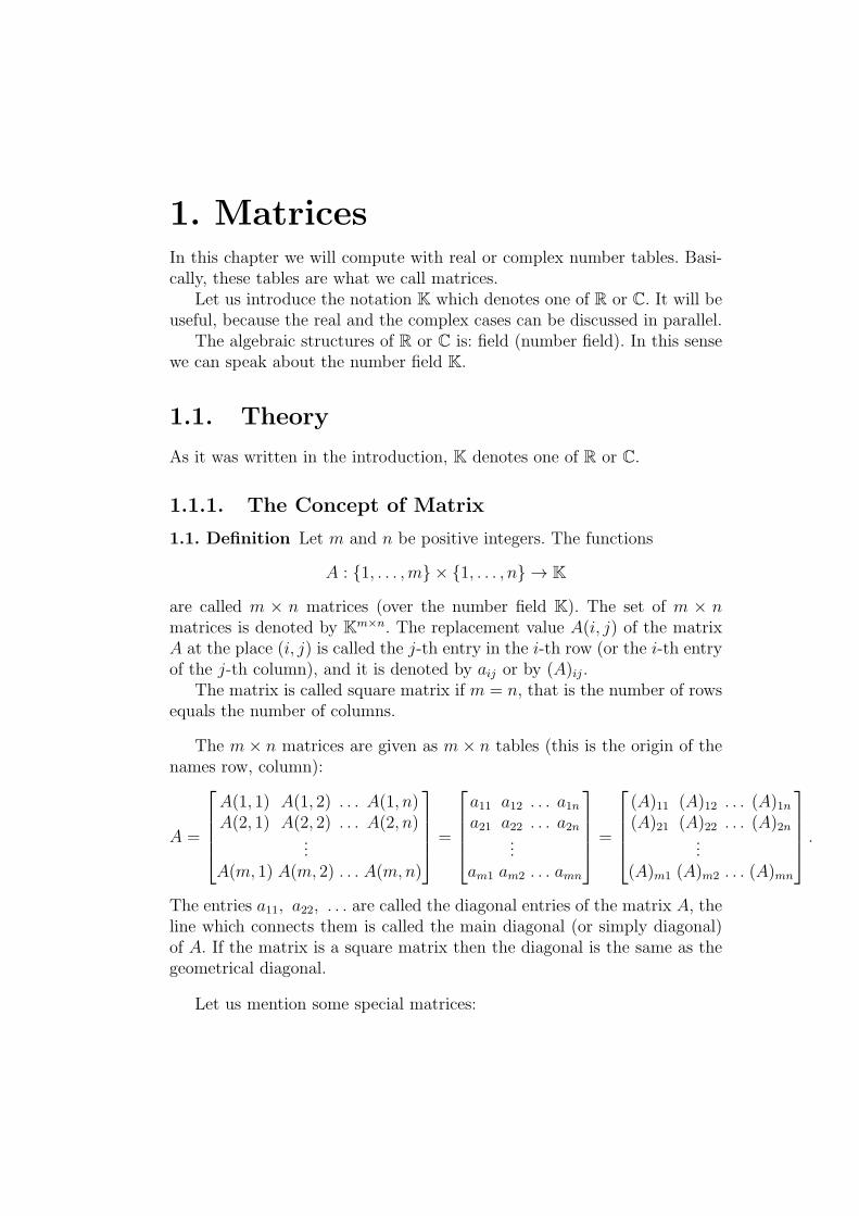
The m× n matrices are given as m× n tables (this is the origin of thenames row, column):

A =

A(1, 1) A(1, 2) . . . A(1, n)A(2, 1) A(2, 2) . . . A(2, n)

...A(m, 1) A(m, 2) . . . A(m,n)

=

a11 a12 . . . a1na21 a22 . . . a2n

...am1 am2 . . . amn

=

(A)11 (A)12 . . . (A)1n(A)21 (A)22 . . . (A)2n

...(A)m1 (A)m2 . . . (A)mn

.

The entries a11, a22, . . . are called the diagonal entries of the matrix A, theline which connects them is called the main diagonal (or simply diagonal)of A. If the matrix is a square matrix then the diagonal is the same as thegeometrical diagonal.

Let us mention some special matrices:

8 1. Matrices

• Zero matrix: all its entries are zero. The zero matrix is often denotedby the symbol 0.

• Row matrix: it has only one row. In other words the elements of K1×n.The row matrices are often called row vectors.

• Column matrix: it has only one column. In other words the elementsof Km×1. The column matrices are often called column vectors.

Later we will speak more about the reason of the names”row vector”,

”column vector” (see Remark 3.8).

• Lower triangular matrix: all the entries above the diagonal are 0, thatis aij = 0 if j > i.

• Upper triangular matrix: all the entries below the diagonal are 0, thatis aij = 0 if j < i.

• Diagonal matrix: all the entries outside of the diagonal are 0, that isaij = 0 if i = j.

Among the square matrices it is important the unit matrix (or identitymatrix):

1.2. Definition The matrix I ∈ Kn×n is called (n × n) unit matrix (oridentity matrix), if:

(I)ij :=

{0 ha i = j,1 ha i = j

(i, j = 1, . . . , n).

1.3. Remark. It is obvious, that the identity matrix is diagonal matrix.

1.1.2. Operations with Matrices

There are several operations which can be made with matrices. The simplestones are the addition and the multplication by scalar. these are performed

”entries”.

1.4. Definition Let A,B ∈ Km×n. The matrix

A+B ∈ Km×n, (A+B)ij := (A)ij +Bij

is called the sum of the matrices A and B.

1.1. Theory 9

1.5. Definition Let A ∈ Km×n and λ ∈ K. The matrix

λA ∈ Km×n, (λA)ij := λ · (A)ij

is called the λ-multiple of the matrix A.

1.6. Theorem The main properties of the above defined matrix operationsare as follows:

I. 1. ∀A,B ∈ Km×n : A+B ∈ Km×n

2. ∀A,B ∈ Km×n : A+B = B + A

3. ∀A,B,C ∈ Km×n : (A+B) + C = A+ (B + C)

4. ∃ 0 ∈ Km×n ∀A ∈ Km×n : A+ 0 = A

(namely, let 0 be the zero matrix)

5. ∀A ∈ Km×n ∃ (−A) ∈ Km×n : A+ (−A) = 0

(namely, let (−A)ij := −(A)ij)

II. 1. ∀λ ∈ K ∀A ∈ Km×n : λA ∈ Km×n

2. ∀A ∈ Km×n ∀λ, µ ∈ K : λ(µA) = (λµ)A

3. ∀A ∈ Km×n ∀λ, µ ∈ K : (λ+ µ)A = λA+ µA

4. ∀A,B ∈ Km×n ∀λ ∈ K : λ(A+B) = λA+ λB

5. ∀A ∈ Km×n : 1A = A

1.7. Remark. The 10 properties listed above are called vector space ax-ioms (see definition 3.1). Thus the vector space axioms hold in Km×n.

The following operation, the product of matrices is a bit more compli-cated.

1.8. Definition Let A ∈ Km×n, B ∈ Kn×p. The matrix

AB ∈ Km×p, (AB)ij := ai1b1j + ai2b2j + . . .+ ainbnj =n∑

k=1

aikbkj

is called the product of the matrices A and B (in this order).

The following properties of the matrix product can be proved by simplecalculations:

10 1. Matrices

1.9. Theorem 1. associative:

(AB)C = A(BC) (A ∈ Km×n, B ∈ Kn×p, C ∈ Kp×q);

2. distributive:

A(B + C) = AB + AC (A ∈ Km×n, B, C ∈ Kn×p);

(A+B)C = AC +BC (A, B ∈ Km×n, C ∈ Kn×p);

3. multiplication by the identity matrix: let I be the unit matrix of rightsize. Then:

AI = A (A ∈ Km×n), IA = A (A ∈ Km×n).

4. multiplication of a product by a scalar:

(λA)B = λ(AB) = A(λB) (A ∈ Km×n, B ∈ Kn×p, λ ∈ K).

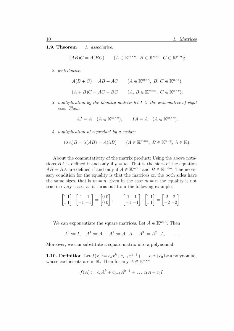
About the commutativity of the matrix product: Using the above nota-tions BA is defined if and only if p = m. That is the sides of the equationAB = BA are defined if and only if A ∈ Km×n and B ∈ Kn×m. The neces-sary condition for the equality is that the matrices on the both sides havethe same sizes, that is m = n. Even in the case m = n the equality is nottrue in every cases, as it turns out from the following example:[

1 11 1

]·[1 1−1 −1

]=

[0 00 0

],

[1 1−1 −1

]·[1 11 1

]=

[2 2−2 −2

].

We can exponentiate the square matrices. Let A ∈ Kn×n. Then

A0 := I, A1 := A, A2 := A · A, A3 := A2 · A, . . . .

Moreover, we can substitute a square matrix into a polynomial:

1.10. Definition Let f(x) := ckxk+ck−1x

k−1+ . . . c1x+c0 be a polynomial,whose coefficients are in K. Then for any A ∈ Kn×n

f(A) := ckAk + ck−1A

k−1 + . . . c1A+ c0I

1.1. Theory 11

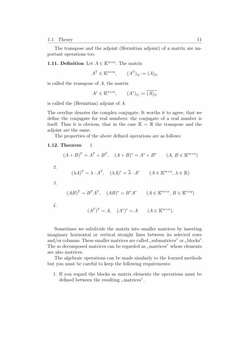
The transpose and the adjoint (Hermitian adjoint) of a matrix are im-portant operations too.

1.11. Definition Let A ∈ Km×n. The matrix

AT ∈ Kn×m, (AT )ij := (A)ji

is called the transpose of A, the matrix

A∗ ∈ Kn×m, (A∗)ij := (A)ji

is called the (Hermitian) adjoint of A.

The overline denotes the complex conjugate. It worths it to agree, that wedefine the conjugate for real numbers: the conjugate of a real number isitself. Thus it is obvious, that in the case K = R the transpose and theadjoint are the same.

The properties of the above defined operations are as follows:

1.12. Theorem 1.

(A+B)T = AT +BT , (A+B)∗ = A∗ +B∗ (A, B ∈ Km×n)

2.(λA)T = λ · AT , (λA)∗ = λ · A∗ (A ∈ Km×n, λ ∈ K)

3.

(AB)T = BTAT , (AB)∗ = B∗A∗ (A ∈ Km×n, B ∈ Kn×p)

4.(AT )T = A, (A∗)∗ = A (A ∈ Km×n).

Sometimes we subdivide the matrix into smaller matrices by insertingimaginary horizontal or vertical straight lines between its selected rowsand/or columns. These smaller matrices are called

”submatrices” or

”blocks”.

The so decomposed matrices can be regarded as”matrices” whose elements

are also matrices.The algebraic operations can be made similarly to the learned methods

but you must be careful to keep the following requirements:

1. If you regard the blocks as matrix elements the operations must bedefined between the resulting

”matrices”.

12 1. Matrices

2. The operations must be defined between the blocks itselves.

In this case the result of the operation will be a partitioned matrix, thatcoincides with the block decomposition of the result of operation with theoriginal (numerical) matrices.

Finally, we speak about an important matrix operation: the inverses ofmatrices. It corresponds to the reciprocal of real or complex numbers.

1.13. Definition Let A, C ∈ Kn×n. The matrix C is called the inverse ofthe matrix A, if

AC = CA = I

(Here I denotes the n× n identity matrix.) The inverse of A is denoted byA−1.

1.14. Definition Let A ∈ Kn×n.(a) The matrix A is called regular (invertible) if it has inverse, that is if

∃A−1.(b) The matrix A is called singular (non-invertible), if it has no inverse,

that is if @A−1.

We can easily prove the uniqueness of the inverse:

1.15. Theorem Let A ∈ Kn×n be a regular matrix, and suppose that bothC ∈ Kn×n and D ∈ Kn×n are the inverses of A, that is

AC = CA = I and AD = DA = I .

Then C = D.

Proof.D = DI = D(AC) = (DA)C = IC = C .

�Thus a square matrix either has no inverse (singular case) or it has only

one inverse (regular case).

We will deal later with the conditions of existence of the inverse andwith the methods of its computation. Here we show an example.[

1 21 3

]−1

=

[3 −2−1 1

],

1.2. Exercises 13

because[1 21 3

]·[3 −2−1 1

]=

[1 00 1

], and

[3 −2−1 1

]·[1 21 3

]=

[1 00 1

].

Thus we have proved that the matrix

[1 21 3

]is regular.

1.1.3. Control Questions to the Theory

1. Define the concept of matrix

2. Define the addition of matrices and list the most important propertiesof this operation

3. Define the scalar multiplication of a matrix and list the most impor-tant properties of this operation

4. Define the product of matrices and list the most important propertiesof this operation

5. Define the Transpose and the Hermitian adjoint of a matrix and listthe most important properties of these operations

1.2. Exercises

1.2.1. Exercises for Class Work

1. What are the sizes of the following matrices? Which of them is zeromatrix, row matrix, column matrix, lower triangular matrix, uppertriangular matrix, diagonal matrix, identity matrix?

A =[1 −1 2 4 3

]; B =

[0 0 0

]; C =

1 0 00 1 00 0 1

;

14 1. Matrices

D =

[2 0 0−3 1 0

]; E =

[71

]; F =

0 0 0 10 0 0 10 0 0 10 0 0 1

.

2. Consider the following matrices:

A =

[−2 1 30 2 5

]; B =

[3 0 21 3 −1

]; C =

[2 45 4

].

Determine (if the result exists):

A+B ; A−B ; 2A−3B ; A+C ; A ·B ; A⊤ ; A⊤ ·C ; C2.

3. Let A =

[1 2−1 2

]∈ R2×2, and let f be the following polynomial:

f(x) := 2x3 − x2 − 5x+ 3 (x ∈ R) .

Compute the matrix f(A).

4. Decide whether C is the inverse of A or not, if

a) A =

[3 −84 6

]; C =

[3 81 3

]

b) A =

1 3 −22 5 −3−3 2 −4

; C =

14 −8 −1−17 10 1−19 11 1

1.2. Exercises 15

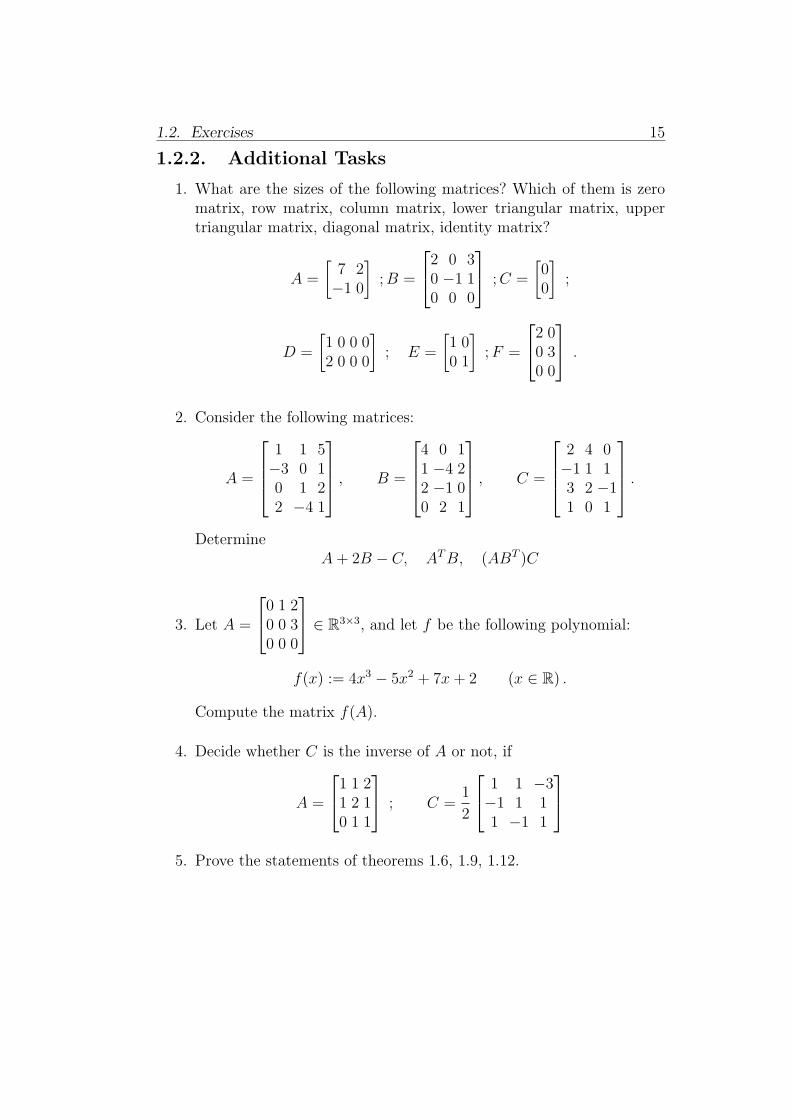
1.2.2. Additional Tasks

1. What are the sizes of the following matrices? Which of them is zeromatrix, row matrix, column matrix, lower triangular matrix, uppertriangular matrix, diagonal matrix, identity matrix?

A =

[7 2−1 0

];B =

2 0 30 −1 10 0 0

;C =

[00

];

D =

[1 0 0 02 0 0 0

]; E =

[1 00 1

];F =

2 00 30 0

.

2. Consider the following matrices:

A =

1 1 5−3 0 10 1 22 −4 1

, B =

4 0 11 −4 22 −1 00 2 1

, C =

2 4 0−1 1 13 2 −11 0 1

.

DetermineA+ 2B − C, ATB, (ABT )C

3. Let A =

0 1 20 0 30 0 0

∈ R3×3, and let f be the following polynomial:

f(x) := 4x3 − 5x2 + 7x+ 2 (x ∈ R) .

Compute the matrix f(A).

4. Decide whether C is the inverse of A or not, if

A =

1 1 21 2 10 1 1

; C =1

2

1 1 −3−1 1 11 −1 1

5. Prove the statements of theorems 1.6, 1.9, 1.12.

2. DeterminantsIn this chapter we’ll get to know the determinants as numbers ordered tosquare matrices. In the light of determinants we will return to the discussionof inverse matrices.

2.1. Theory

As we have agreed K denotes one of the number sets R or C, that is K ∈{R, C}.

2.1.1. The Concept of Determinant

To the definition of determinant we need minor matrices via deleting onerow and one column of a square matrix:

2.1. Definition Let n ≥ 2 and A ∈ Kn×n and (i, j) be a pair of row-columnindices (i, j ∈ {1, . . . , n}). Delete the i-th row and the j-th column fromA. The remainder (n− 1)× (n− 1)-size matrix is called the minor matrixof A related to the index pair (i, j). This minor matrix is denoted by Aij.

After these preliminaries we define recursively the function det : Kn×n →K as follows:

2.2. Definition 1. If A = [a11] ∈ K1×1, then det(A) := a11.

2. If A ∈ Kn×n, then:

det(A) :=n∑

j=1

a1j · (−1)1+j · det(A1j) =n∑

j=1

a1j · a′1j,

where a′ij := (−1)i+j ·det(Aij), and it is called: signed subdeterminantor cofactor.

We say that we have defined the determinant by expansion along the firstrow.

2.3. Examples

2.1. Theory 17

1. The determinant of a 2× 2 matrix can be computed as follows:

det(

[a bc d

]) = a · (−1)1+1 · det([d]) + b · (−1)1+2 · det([c]) = ad− bc,

that is we obtain the determinant of a 2 × 2 matrix if we subtractfrom the product of its main diagonal entries the product of its sidediagonal entries.

2. It follows immediately from the definition, that the determinant of alower diagonal matrix (especially a diagonal matrix) equals the prod-uct of its diagonal elements. Consequently, the determinant of theidentity matrix equals 1.

In addition to det(A) we will use the notation∣∣∣∣∣∣∣∣∣a11 . . . a1na21 . . . a2n...

...an1 . . . ann

∣∣∣∣∣∣∣∣∣also for the determinant. We speak in this sense about the rows, the columns,the entries etc. of the determinant.

Thus, using the above notation:∣∣∣∣a11 a12a21 a22

∣∣∣∣ = a11a22 − a12a21

Hereinafter we list - without proof - some important and useful proper-ties of the determinant.

1. The determinant can be expanded by its any row or its any column,that is for any r, s ∈ {1, . . . , n} holds:

det(A) =n∑

j=1

arj · a′rj =n∑

i=1

ais · a′is.

2. The consequence of the previous statement is that det(A) = det(AT ).It follows from here, that the determinant of an upper triangular ma-trix equals the product of its main diagonal entries.

18 2. Determinants

3. If a determinant has only 0 entries in a row (or in a column), then itsvalue equals 0.

4. If we swap two rows (or two columns) of a determinant, then its valuewill be the opposite of the original one.

5. If a determinant has two equal rows (or two equal columns), then itsvalue equals 0.

6. If we multiply every entry of a row (or of a column) of the determinantby a number λ, then its value will be the λ-multiple of the originalone.

7. ∀A ∈ Kn×n and ∀λ ∈ K holds det(λ · A) = λn · det(A).

8. If two rows (or two columns) of a determinant are proportional, thenits value equals 0.

9. The determinant is additive in its any row (and by its any column).This means – in the case of additivity of its r-th row – that:

If (A)ij :=

αj if i = r

aij if i = r,and (B)ij :=

βj if i = r

aij if i = r,

and (C)ij :=

αj + βj if i = r

aij if i = r ,

then det(C) = det(A) + det(B).

10. If we add to a row of a determinant a scalar multiple of another row(or to a column a scalar multiple of another column), then the valueof the determinant remains unchanged.

11. The determinant of the product of two matrices equals the product oftheir determinants:

det(A ·B) = det(A) · det(B) (A, B ∈ Kn×n) .

The determinant is in close connection with the calculation of length, ofarea and of volume. We write more about this topic in the Appendix, seethere

”The geometric meaning of the determinant”.

2.1. Theory 19

2.1.2. Inverses of Matrices

In the definition 1.13 the concept of the inverse matrix was defined, furtherit was proved its uniqueness.

In this section – using the determinant – we investigate in more detailthe conditions of the existence of inverse matrix.

2.4. Theorem [existence of the right-hand inverse]Let A ∈ Kn×n. Then there exists a matrix C ∈ Kn×n for which holds

AC = I if and only if det(A) = 0. Such a matrix C is called a right-handinverse of A.

Proof. First suppose the existence of C with this property. Then AC = I,consequently:

1 = det(I) = det(A · C) = det(A) · det(C).

From here immediately follows det(A) = 0.Conversely, suppose det(A) = 0. Define the following matrix:

C :=1

det(A)· A , ahol (A)ij := a′ji .

Now we will show that AC = I holds for this C. Really:

(AC)ij =

(A · 1

det(A)· A)

ij

=1

det(A)· (A · A)ij =

=1

det(A)·

n∑k=1

(A)ik · (A)kj =1

det(A)·

n∑k=1

aik · a′jk.

The last sum equals 1 if i = j, because – using the expansion of the deter-minant along the i-th row:

1

det(A)·

n∑k=1

aik · a′ik =1

det(A)· det(A) = 1.

Now suppose that i = j. In this case the above mentioned sum is theexpansion of a determinant along its j-th row which can be obtained fromdet(A) by exchanging its j-th row to its i-th row. But this determinant hastwo equal rows (the i-th and the j-th), so its value equals 0. This meansthat

∀ i = j : (AC)ij = 0 .

20 2. Determinants

We have proved that (AC)ij = (I)ij, consequently the product AC reallyequals the identity matrix. �

Using the theorem about the right-hand inverse, it can be proved theexistence of the inverse matrix.

2.5. Theorem Let A ∈ Kn×n. Then

∃A−1 ⇐⇒ det(A) = 0 ,

that is the matrix A is regular if and only if det(A) = 0. Consequently, thematrix A is singular if and only if det(A) = 0.

Proof. First suppose that A is regular, that is ∃A−1. Then A · A−1 = I,thus

1 = det(I) = det(A · A−1) = det(A) · det(A−1) .

This implies det(A) = 0. Furthermore we have

det(A−1) =1

det(A).

Conversely, suppose det(A) = 0. Then – usig the second half of theprevious theorem – there exists a matrix C ∈ Kn×n, for which holds AC = I.

We will show, that this matrix C is the inverse of A. Since AC = I isproved (see the previous theorem), it is enough to prove that CA = I.

This is proved as follows. Since det(AT ) = det(A) = 0, we can apply thesecond half of the previous theorem for the matrix AT . Thus we have

∃D ∈ Kn×n : ATD = I .

Let us transpose both sides of the equality:

(ATD)T = IT ,

form where DTA = I follows. With the help of this fact the equality CA = Iwill be proved easily:

CA = ICA = DTACA = DT (AC)A = DT IA = DTA = I .

�

2.6. Remarks.

2.1. Theory 21

1. We emphasize once more time, that the regularity of a matrix A ∈Kn×n is equivalent with the fact that its determinant is nonzero. Inthe regular case we have deduced an explicit formula for the inverse:

A−1 =1

det(A)· A , where (A)ij := a′ji .

2. Let us apply the previous result for the 2× 2 matrix

A =

[a bc d

]∈ R2×2 .

Then A is regular if and only if ad − bc = 0. In this case the inversematrix is

A−1 =1

ad− bc·[d −b−c a

].

Expressing it in words:

We obtain the inverse of a 2× 2 regular matrix if we interchange theentries in its main diagonal, then we change the signs of the entriesin the side diagonal, finally, we multiply the obtained matrix with thereciprocal of the determinant of the original matrix.

3. It follows from our considerations, that to prove that the inverse ofA ∈ Kn×n is the matrix C ∈ Kn×n it is enough to prove only one ofthe equalities AC = I or CA = I. The other one holds automatically.


1. Define the concept of the minor matrix assigned to the index pair(i, j) of an m× n matrix, and give a numerical example for this

2. Define the concept of determinant

3. Define the concept of cofactor assigned to (i, j)

4. How can we compute the 2× 2 determinants?

5. How can we compute the determinant of a triangular matrix?

22 2. Determinants

6. State the following properties of the determinant:

- expansion along any row/column

- transpose-property

- 0 row/column

- row/column interchange property

- two rows/two columns are equal

- row/column homogeneous

- the determinant of λA

- proportional rows/columns

- row/column additive

- the determinant of AB

7. Define the right-hand inverse, the left-hand inverse and the inverse ofa square matrix

8. Define the concept of singular matrix and regular matrix

9. State and prove the theorem about the existence and formula of theright-hand inverse

10. State and prove the theorem about the necessary and sufficient con-dition of the existence of the left-hand inverse (reducing the problemback to the right-hand inverse)

11. State and prove the theorem about the connection between the right-hand and the left-hand inverses

12. State and prove the statement about the existence and formula of theinverse

13. State and prove the formula of the inverse of a 2× 2 matrix

2.2. Exercises 23

2.2. Exercises


1. Let

a) A =

[1 23 4

]∈ R2×2 b) A =

3 1 −42 5 61 4 8

∈ R3×3

(1) Compute detA in different ways.

(2) Determine whether the matrix A is regular or singular. In theregular case determine the inverse of A using cofactors.

(3) Check A · A−1 = I.

2. The following matrices are regular or singular? In regular case deter-mine the inverse matrix.

A =

[−2 5−3 1

]B =

[−2 3−4 6

]

3. Illustrate the properties of determinants with concrete matrices.


1. Compute the following determinants:

a)

∣∣∣∣∣∣3 1 −42 5 61 4 8

∣∣∣∣∣∣ b)

∣∣∣∣∣∣∣∣1 0 0 −13 1 2 21 0 −2 12 0 0 1

∣∣∣∣∣∣∣∣

24 2. Determinants

2. Determine the inverse matrices:

a)

[4 −5−2 3

]b)

3 2 −11 6 32 −4 0

furthermore check the result by the definition of the inverse matrix.

3. Illustrate the properties of determinants with concrete matrices.

4. Let A ∈ Kn×n be a diagonal matrix (that is aij = 0 if i = j). Provethat it is invertible if and only if none of the diagonal elements equals0. Prove that in this case A−1 is a diagonal matrix with diagonalelements

1

a11,

1

a22, . . .

1

ann.

3. Vectors, Vector SpacesIn this chapter the concept of vector will be generalized.

3.1. Theory

3.1.1. The Concept of Vector Space

In the secondary school we got acquainted with the concept of vector, op-erations with vectors and their properties. We have found, that the vectoraddition has the following properties:

1. If a and b are vectors then a+ b is also a vector

2. a+ b = b+ a (commutative law)

3. (a+ b) + c = a+ (b+ c) (associative law)

4. a+ 0 = a (the characterization of the zero vector)

5. a+ (−a) = 0 (the characterization of the opposite vector)

The most important properties of the multiplication of vectors by ascalar are follows:

1. If λ is a real number, and a is a vector, then λa is a vector

2. λ(µa) = (λµ)a (multiply a product)

3. (λ+ µ)a = λa+ µa (distributive law)

4. λ(a+ b) = λa+ λb (distributive law)

5. 1a = a

We have seen the same properties in connection with matrices in Theo-rem 1.6.

Now we generalize the concept of vector in the following way: we takea nonempty set (whose elements will be called vectors), and we take anumber set (which will be called scalar range and whose elements will becalled scalars). Furthermore we take two operations (addition of vectors

26 3. Vectors, Vector Spaces

and multiplication of vectors by scalars), which have the above written10 features. The resulting

”structure” will be called vector space. The 10

features are called vector space axioms.

We will use the number fields R and C as scalar range, that is, the scalarrange will be the number field K. Thus we can investigate the real and thecomplex vector spaces

”in parallel”.

After this introduction let us see the definition of a vector space:

3.1. Definition Let V = ∅. We say, that V is a vector space over K ifthere exist the operations x + y (addition) and λx = λ · x (multiplicationby scalar) so that the following axioms hold

I. 1. ∀ (x, y) ∈ V × V : x+ y ∈ V

2. ∀ x, y ∈ V : x+ y = y + x

3. ∀ x, y, z ∈ V : (x+ y) + z = x+ (y + z)

4. ∃ 0 ∈ V ∀ x ∈ V : x+ 0 = x

It can be proved that 0 is unique. Its name is: zero vector.

5. ∀ x ∈ V ∃ (−x) ∈ V : x+ (−x) = 0

It can be proved that (−x) is unique. Its name is: the oppositeof x.

II. 1. ∀ (λ, x) ∈ K× V : λx ∈ V

2. ∀ x ∈ V ∀λ, µ ∈ K : λ(µx) = (λµ)x = µ(λx)

3. ∀ x ∈ V ∀λ, µ ∈ K : (λ+ µ)x = λx+ µx

4. ∀ x, y ∈ V ∀λ ∈ K : λ(x+ y) = λx+ λy

5. ∀ x ∈ V : 1x = x

The elements of V are called vectors, the elements of K are called scalars.K is called the scalar region (scalar range) of V .

Applying several times the associative law of addition we can define thesums of several terms:

x1 + x2 + · · ·+ xk =k∑

i=1

xi (xi ∈ V ) .

3.2. Remarks.

3.1. Theory 27

1. The vectors are often denoted by underlined lowercases , but it is notrequired.

2. It is in evidence, that the axioms are derived from the properties ofgeometric vectors studied in secondary school. Thus we have our firstexample for vector space:

The plane vectors starting from a fixed point of the plane form a vectorspace over R, with respect to the common vector addition and multi-plication by scalar.

The fixed starting point is necessary, so there won’t be any problemwith the equality of vectors.

3. Sometimes we use the operations”multiplication by scalar from the

right”,”division by a nonzero number”,

”subtraction” as follows:

x · λ := λ · x, x

λ:=

1

λ· x x− y := x+ (−y).

The properties of these operations follow from the axioms.

4. If the scalar region and the two operations are given by some defaultsetting, then we simply say:

”V is a vector space”.

3.3. Examples

1. The vectors in the plane, with the usual vector operations form avector space over R. This is the vector space of plane vectors. Sincethe plane vectors can be identified with the points of the plane, insteadof the vector space of the plane vectors we can speak about the vectorspace of the points in the plane.

2. The vectors in the space, with the usual vector operations form avector space over R. This is the vector space of space vectors. Sincethe space vectors can be identified with the points of the space, insteadof the vector space of the space vectors we can speak about the vectorspace of the points in the space.

3. From the algebraic properties of the number field K immediately fol-lows that R is vector space over R, C is vector space over C, that isK is vector space over K.

As a matter of fact, note that C is vector space over R too.

4. For fixed m,n ∈ N+ the set of m× n matrices, that is Km×n forms avector space over K. This follows immediately from Theorem 1.6.


5. The one-element-set is vector space over K. Since the single elementof this set must be the zero vector of the space, we will denote thisvector space by {0}. The operations in this space are:

0 + 0 := 0, λ · 0 := 0 (λ ∈ K) .

The name of this vector space is: zero vector space.

If we don’t say anything else, the symbol V will denote a vector space overK.

In the following theorem some basic properties of vector spaces will belisted. They can be prove using the axioms.

3.4. Theorem Let x ∈ V, λ ∈ K. Then

1. 0 · x = 0 (the left hand side 0 denotes the number zero in K, the righthand side 0 denotes the zero vector in V )

2. λ · 0 = 0 (here both 0-s denote the zero vector in V )

3. (−1) · x = −x.

4. λ · x = 0 ⇐⇒ λ = 0 or x = 0.

3.1.2. The Vector Space Kn

This section will be about a very important vector space: about Kn.For a fixed n ∈ N+ the function

x : {1, . . . , n} → K

is called an n-term sequence ( in other words: ordered n-tuple) created fromthe elements of K.

The number x(i) ∈ K is called the i-th component of the vector x, andit is denoted by xi (i = 1, . . . , n). The n-tuple itself is denoted as follows:

x = (x1, x2, . . . xn) .

E. g. (1, −3, 5, 8) is an ordered 4-tuple.

Let us denote the set of all n-tuples constructed from the elements of Kby Kn:

3.1. Theory 29

Kn := {x = (x1, x2, . . . , xn) | xi ∈ K}

Following the previous example e.g. (1, −3, 5, 8) ∈ R4.

Let us define the operations”componentwise”:

(x1, x2, . . . , xn) + (y1, y2, . . . , yn) := (x1 + y1, x2 + y2, . . . , xn + yn) ;

λ · (x1, x2, . . . , xn) := (λx1, λx2, . . . , λxn) (λ ∈ K) .

In another way:

(x+ y)i := xi + yi; and (λ · x)i := λ · xi (i = 1, . . . , n; x, y ∈ Kn).

3.5. Theorem Kn is a vector space over the number field K.The zero vector of this vector space is the n-tuple (0, 0, . . . , 0), the op-

posite of the vector (x1, x2, . . . , xn) is (−x1, −x2, . . . , −xn).

Proof. One can easily check the validity of the 10 axioms. �

The conventional way for writing the elements of Kn is:

x = (x1, x2, . . . , xn) ∈ Kn ,

but sometimes it is useful to write them in column-mode:

x =

x1

x2...xn

∈ Kn .

The column-mode writing is usefol e.g. in the case when we perform alge-braic operations with elements in Kn. In this case the components havingthe same indices stand at the same height. Thus they are better manageable.For example in R4 we have:

2 ·

−1251

+ 3 ·

12−32

=

2 · (−1) + 3 · 12 · 2 + 3 · 2

2 · 5 + 3 · (−3)2 · 1 + 3 · 2

=

11018

.


3.6. Remark. If we speak about the vector space Kn then the defaultscalar region is K and the default operations are the componentwise oper-ations.

3.7. Remark. It is known that the points and the vectors in the plane canbe characterized by number pairs. Similarly, the points in the space and thevectors in the space can be characterized by number triples. Thus R2 canbe considered the vector space of the points of the plane, or of the vectorsof the plane. Similarly, R3 can be considered the vector space of the pointsof the space, or of the vectors of the space.

Using similar justification, R = R1 can be considered the vector spaceof the points of the line (number line).

3.8. Remark. The vector space Kn can be identified with the space ofrow matrices K1×n, moreover, it can be identified with the space of columnmatrices Kn×1 too. This is the reason, that the row matrices are sometimescalled

”row vectors”, the column matrices are called sometimes

”column

vectors”.

As a special case of matrix product, we can define the matrix-vectorproduct operation as follows:

3.9. Definition Let A ∈ Km×n, x ∈ Kn. The vector

Ax ∈ Km, (Ax)i := ai1x1+ai2x2+. . .+ainxn =n∑

j=1

aijxj (i = 1, . . . ,m)

is called the product of matrix A and vector x (in this order).

3.10. Remark. One can see, that we can compute vector Ax in the fol-lowing way: multiply matrix A by the column matrix associated to x, andtake of as a result the vector associated to the column matrix we computed.This will be Ax. Thus the matrix-vector product is essentially a product ofa matrix and a column matrix. This identification implies in a natural waythe properties of the matrix-vector product.

3.1.3. Subspaces

3.11. Definition Let W be a nonempty subset of the vector space V . Wesay that W is a subspace of V (or: W is a subspace in V ), if W is a vectorspace regarding the operations of V .

3.1. Theory 31

The following theorem gives a useful method to decide whether a subsetin V is a subspace or not.

3.12. Theorem Let W ⊂ V, W = ∅.W is a subspace of V if and only if the following two assumptions hold:

1. ∀x, y ∈ W : x+ y ∈ W ,

2. ∀x ∈ W ∀λ ∈ K : λx ∈ W .

The first assumption expresses that W is closed under addition. Similarly,the second assumption expresses that W is closed under scalar multiplica-tion.

Proof. The two given assumptions are obviously necessary.To prove that they are sufficient, let us realize that the vector space

axioms I.1. and II.1. are exactly the given conditions so they are true.Moreover, axioms I.2., I.3., II.2., II.3., II.4., II.5. are identities, so they areinherited from V to W .

It remains us to prove only two axioms: I.4., I.5.Proof of I.4.: Let x ∈ W and 0 be the zero vector in V . Then – because

of the second condition: 0 = 0x ∈ W , so W really contains a zero vector,and the zero vectors in V and W are the same.

Proof of I.5.: Let x ∈ W and −x be the the opposite vector of x inV . Then – also because of the second condition: −x = (−1)x ∈ W , so Wreally contains an opposite of x and the opposite vectors in V and W arethe same.

�

3.13. Corollary. It follows immediately from the above proof, that a sub-space must contain the zero vector of V . In other words: if a subset does notcontain the zero vector of V , then it is not a subspace. Similar considerationsare valid for the opposite vector too.

Using the above theorem one can easily prove that the following exam-ples are subspaces.

3.14. Examples

1. The zero vector space {0} and V itself both are subspaces in V . Theyare called the trivial subspaces.

2. All the subspaces of the vector space of plane vectors (R2) are:


- the zero vector space {0},

- the straight lines trough the origin,

- R2 itself.

3. All the subspaces of the vector space of space vectors (R3) are:

- the zero vector space {0},

- the straight lines trough the origin,

- the planes trough the origin,

- R3 itself.


1. Define the concept of a vector spaces

2. Give 2 examples for vector space

3. State the 4 elementary properties of vector spaces

4. Define the vector space Kn (its elements, operations in it)

5. Define the matrix-vector product operation

6. Define the subspace of a vector space

7. State and prove the theorem about the necessary and sufficient con-dition for a set to be a subspace

8. Give 2 examples for subspaces

3.2. Exercises 33

3.2. Exercises


1. Let us give the following vectors in R5:

x = (−3, 4, 1, 5, 2) y = (2, 0, 4,−3,−1) z = (7,−1, 0, 2, 3) ,

and the matrix

A =

[5 1 −4 −2 10 2 4 −3 −1

]∈ R2×5 .

Compute:

x+ y , y − z , 4x , x+ 3y − 2z , Ax .

2. Are the following sets subspaces in R2 or not? Which famous sets ofpoints are they (give their geometric names)?

K := {(x, y) ∈ R2 | x2+y2 = 1} ; N := {(x, y) ∈ R2 | x ≥ 0 y ≥ 0} .

3. Are the following sets subspaces in R3 or not? Give their geometricnames.

(a) S1 = {(x, y, z) ∈ R3 | x2 + y2 + z2 = 1},

(b) S2 = {(x, y, z) ∈ R3 | x ≥ 0, y ≥ 0, z ≥ 0},

(c) S3 = {(x, y, z) ∈ R3 | 2x− 3y + z = 0},

(d) S4 = {(x, y, z) ∈ R3 | 2x− 3y + z = 5},

(e) S5 = {(x− y, 3x, 2x+ y) ∈ R3 | x, y ∈ R}.

4. Prove, that the vector space axioms hold in Kn.



1. Consider the following vectors

x = (1,−2, 3, 4) ∈ R4 , y = (−4, 0, 2, 1) ∈ R4 , z = (2,−1, 0) ∈ R3 ,

and the matrix

A =

3 1 2−1 1 −20 2 42 −1 0

∈ R4×3

Compute:3x+ y + 2Az

2. Are the following sets subspaces in R2 or not? Which famous sets ofpoints are they (give their geometric names)?

K := {(x, y) ∈ R2 | xy = 1} ; N := {(x, y) ∈ R2 | xy ≥ 0} .

3. Are the following sets subspaces in R3 or not? Give their geometricnames.

(a) S1 = {(x, y, z) ∈ R3 | z = x2 + y2},(b) S2 = {(x, y, z) ∈ R3 | z2 = x2 + y2},(c) S3 = {(2x, x+ y, y) ∈ R3 | x, y ∈ R}.(d) S4 = {(x, y, z) ∈ R3 | 4x− y + 3z = 0},(e) S5 = {(x, y, z) ∈ R3 | 4x− y + 3z + 1 = 0},

4. Prove, that the vector space axioms hold in Kn (continuation of aclass-work-exercise).

4. Geneated SubspacesIn this section we will give subspaces with the help of some vectors of afinite number.

4.1. Theory

From now on, it will be often mentioned the concept of a (finite) vectorsystem. We speak about a (finite) vector system, if we choose a finite numberof vectors from a vector space in the way, that some vectors may be chosenseveral times. This

”chosen several times” option is exactly the reason why

we make a distinction between a vector system and a set of vectors.

4.1.1. Linear Combination

4.1. Definition Let k ∈ N+, x1, . . . , xk ∈ V be a vector system, λ1, . . . λk ∈K. The vector

λ1x1 + · · ·+ λkxk =k∑

i=1

λixi

(or the expression itself) is called the linear combination of the vector systemx1, . . . , xk, with the coefficients λ1, . . . λk.

The linear combination is called trivial, if all its coefficients are zero,and it is called nontrivial, if it has at least one nonzero coefficient.

Obviously, the result of a trivial linear combination is always the zerovector.

4.2. Remark. Using mathematical induction, it can be proved, that if W

is a subspace in V , and x1, . . . , xk ∈ W , λ1, . . . λk ∈ K, thenk∑

i=1

λixi ∈ W ,

that is: subspaces are closed under linear combination.

4.1.2. The Concept of Generated Subspace

Let x1, x2, . . . , xk ∈ V be a vector system. Consider the following subsetof V :

W ∗ := {k∑

i=1

λixi ∈ V | λ1, . . . , λk ∈ K} . (4.1)

36 4. Geneated Subspaces

One can see that the elements of W ∗ are all the possible linear combinationsof the vector system x1, x2, . . . , xk.

4.3. Theorem 1. W ∗ is a subspace in V .

2. W ∗ covers the system x1, x2, . . . , xk, which means that

xi ∈ W ∗ (i = 1, . . . , k) .

3. For any subspace Z ⊆ V which covers (in the above sense) the systemx1, x2, . . . , xk, holds W ∗ ⊆ Z.

Note before the proof, that the statement of this theorem is shortly sayingthat W ∗ is the minimal subspace, which covers x1, x2, . . . , xk.Proof.

1. Let a =k∑

i=1

λixi ∈ W ∗ and b =k∑

i=1

µixi ∈ W ∗. Then

a+ b =k∑

i=1

λixi +k∑

i=1

µixi =k∑

i=1

(λi + µi)xi ∈ W ∗ .

Furthermore, for any λ ∈ K holds

λa = λk∑

i=1

λixi =k∑

i=1

(λλi)xi ∈ W ∗ .

Consequently, W ∗ is really a subspace in V .

2. For any fixed index i ∈ {1, . . . , k} holds

xi = 0x1 + . . . + 0xi−1 + 1xi + 0xi+1 + . . . + 0xk ∈ W ∗ .

3. Let Z be a subspace given in the theorem, and let a =k∑

i=1

λixi ∈ W ∗.

Since Z covers the vector system, then

xi ∈ Z (i = 1, . . . , k) .

But Z is a subspace, therefore it is closed under linear combination.It implies that a ∈ Z. So really W ∗ ⊆ Z.

�

4.1. Theory 37

4.4. Definition The subspace W ∗ defined in (4.1) is called the subspacegenerated (or spanned) by the vector system x1, x2, . . . , xk. It is denotedby Span (x1, x2, . . . , xk).

4.5. Definition Let W be a subspace of V . We say that W has a finitegenerator system if

∃ k ∈ N+ ∃x1, x2, . . . , xk ∈ V : Span (x1, x2, . . . , xk) = W .

In this case the vector system x1, x2, . . . , xk is called a (finite) generatorsystem of the subspace W .

4.6. Definition In the case when Span (x1, x2, . . . , xk) = V the vectorsystem x1, x2, . . . , xk is called simply generator system.

4.7. Remark. The fact, that a vector x lies in the subspace generated bythe vectors x1, . . . , xk is equivalent with the fact, that x can be written asa linear combination of vectors x1, . . . , xk. We can also say that vector xlinearly depends on vectors x1, . . . , xk.

4.8. Examples

1. Let v be a fixed vector in the space of plane vectors. Then

Span (v) =

{{0} if v = 0,v a straight line through the origin with direction vector v if v = 0.

One can easily prove that in the space of the plane vectors any twononparallel vectors are forming a generator system.

2. In the space of space vectors let v1 and v2 be two fixed vectors. Then

Span (v1, v2) =

{0} if v1 = v2 = 0,the common straight line of v1 and v2 if v1 ∥ v2the common plane of v1 and v2 if v1 ∦ v2.

It can be easily proved, that in the space of space vectors any threevectors, which are not contained in the same plane are forming agenerator system.

3. The i-th canonical unit vector (or standard unit vector) in Kn – letus denote it by ei – is defined as follows:

Let the i-th component of ei be 1, and all its other components to be0 (i = 1, . . . , n).


Then the vector system e1, . . . , en is a generator system in Kn, becausefor any x = (x1, . . . , xn) ∈ Kn holds

x =

x1

x2...xn

=

x1 · 1 + x2 · 0 + · · ·+ xn · 0x1 · 0 + x2 · 1 + · · ·+ xn · 0

...x1 · 0 + x2 · 0 + · · ·+ xn · 1

=

= x1 ·

10...0

+ x2 ·

01...0

+ · · ·+ xn ·

00...1

=n∑

i=1

xiei

Thus x really can be written as a linear combination of the standardunit vectors e1, . . . , en.

4.9. Remark. It is clear, that if we enlarge a generator system in V , thenit still remains a generator system. But if we leave vectors from a generatorsystem, then the result system may not necessarily stay a generator system.The generator systems are – in this sense – the

”large” systems. Later we

will study the question of”minimal” generator systems.

4.1.3. Finite Dimensional Vector Space

The concept of a generator system can be extended into an infinite systemas well. In this connection, we call the above defined generator system moreprecisely a finite generator system. An important class of vector spaces arethe spaces having a finite generator system.

4.10. Definition The vector space V is called finite-dimensional if it hasfinite generator system, that is, if

∃ k ∈ N+ ∃ x1, x2, . . . , xk ∈ V : Span (x1, x2, . . . , xk) = V .

The fact, that V is a finite dimensional space is denoted by dimV < ∞.

4.11. Definition The vector space V is called infinite-dimensional if itdoes not have a finite generator system, that is, if

∀ k ∈ N+ ∀ x1, x2, . . . , xk ∈ V : Span (x1, x2, . . . , xk) = V .

The fact, that V is infinite dimensional is denoted by dimV = ∞.

4.1. Theory 39

4.12. Examples

1. The space of the plane vectors is finite dimensional. A finite generatorsystem is i, j.

2. The space of space vectors is finite dimensional. A finite generatorsystem is i, j, k.

3. The space Kn is finite dimensional. A finite generator system is thesystem of the n standard unit vectors.

4. You can find an example for an infinite dimensional vector space inthe Appendix.


1. Define the linear combination

2. State and prove the theorem about a generated subspace by a finitevector system (This is the theorem about W ∗)

3. Give 2 examples for generated subspaces in R2

4. Give 2 examples for generated subspaces in R3

5. Define the standard unit vectors in Kn. What is the subspace gener-ated by them?

6. Define the notion of a finite dimensional vector space. Why is thevector space Kn finite dimensional?

7. Define the notion of an infinite dimensional vector space.


4.2. Exercises


1. Write the subspace

W := Span ((1, 2,−1), (−3, 1, 1)) ⊆ R3

as a set. Give several elements of this subspace.

Determine whether the vectors (2, 4, 0) and (5,−4,−1) are containedin this subspace or not.

2. Consider the following vectors in R3:

u = (1, 2,−1) ; v = (6, 4, 2) ; x = (9, 2, 7) ; y = (4,−1, 8).

(a) Compute the result of the linear combination −2u+ 3v.

(b) Write up the elements of the subspace Span (u, v).

(c) Determine whether x ∈ Span (u, v) or not.

(d) Determine whether y ∈ Span (u, v)ornot.

3. Consider the subspaces

(a) S5 = {(x− y, 3x, 2x+ y) ∈ R3 | x, y ∈ R} ⊆ R3 ,

(b) S3 = {(x, y, z) ∈ R3 | 2x− 3y + z = 0} ⊆ R3

and the subspaces

(c) W1 = {(x− y+5z, 3x− z, 2x+ y− 7z,−x) ∈ R4 | x, y, z ∈ R} ⊆R4 ,

(d) W2 = {(x, y, z) ∈ R3 | x+ 3y = 0} ⊆ R3

discussed on the previous practice. Determine (finite) generator sys-tems to each of them.

Remark: If it is possible to write the elements of the set as linearcombinations of a finite generator system, then it proves that the setis really a subspace. Thus this is a new possibility to prove, that a setis a subspace.

4. Determine (finite) generator systems for the following subspaces inR3:

4.2. Exercises 41

(a) W1 = {(x, y, z) ∈ R3 |[2 −3 5

]·

xyz

=(0)},

(b) W2 = {(x, y, z) ∈ R3 |[1 −2 32 0 −1

]·

xyz

=

(00

)},

(c) W3 = {(x, y, z) ∈ R3 |[2 −1 −2−4 2 4

]·

xyz

=

(00

)}.

Remark: Considering the remark of the previous exercise, it is unnec-essary to justify forward that the given sets are really subspaces.

5. Determine a (finite) generator system of the following subspace in R4:

W = {(2x−y+z, y+3z, x+y−2z, x−y) ∈ R4 | x, y, z ∈ R, x+2y+z = 0} ⊆ R4 .

Remark: Here it is also unnecessary to justify forward that the givenset is really a subspace.


1. Consider the vectors a = (1, 2,−1), b = (−3, 1, 1) ∈ R3.

(a) Compute the vector 2a− 4b.

(b) Write up several elements of the subspace Span (a, b).

(c) Determine whether the vectors x = (2, 4, 0), y = (2, 4,−3) arecontained in Span (a, b) or not.

2. Determine (finite) generator systems for the following subspaces:

(a) W1 = {(x− y, x+ 2y, 3x, 4x+ 3y) ∈ R4 | x, y ∈ R} ⊆ R4

(b) W2 = {(x, 5x,−4x, 7x) ∈ R4 | x ∈ R} ⊆ R4

(c) W3 = {(x, y, z, u) ∈ R4 | x− 2y + 4z + 3u = 0} ⊆ R4

(d) W4 = {(x, y, z, u) ∈ R4 | 2x− 3z = 0} ⊆ R4


(e) W5 = {(x, y, z) ∈ R3 |[4 −1 2

]·

xyz

=(0)} ⊆ R3,

(f) W6 = {(x, y, z) ∈ R3 |[1 −1 43 1 2

]·

xyz

=

(00

)} ⊆ R3,

(g) W7 = {(x, y) ∈ R2 |

1 23 6−1 −2

·(xy

)=

000

} ⊆ R2.

3. Determine a (finite) generator system of the following subspace in R4:

W = {

x+ y + u

3x− 2y + 5z − u2x+ 2z − u3z + 2u

∈ R4 | x, y, z, u ∈ R, x+y+z+u = 0} ⊆ R4 .

5. Linear Independence

5.1. Theory

5.1.1. The Concept of Linear Independence

5.1. Definition Let k ∈ N+ and x1, . . . , xk ∈ V be a vector system in thevector space V . This vector system is called linearly independent (shortly:independent), if among its possible linear combinations only the trivial lin-ear combination results the zero vector. That is, if

k∑i=1

λixi = 0 =⇒ λ1 = λ2 = . . . = λk = 0 .

The vector system is called linearly dependent (shortly: dependent) if it isnot independent, that is if:

∃λ1, λ2, . . . λk ∈ K, λi not all 0 :k∑

i=1

λixi = 0 .

5.2. Remarks.

1. The equationk∑

i=1

λixi = 0 is called dependence equation (or: depen-

dence relation).

2. One can simply prove, that a vector system containing the zero vectoror containing identical vectors is linearly dependent. Consequently, alinearly independent system cannot contain neither the zero vector,nor identical vectors.

3. The one-term vector system is linearly independent if and only if itssingle vector is not the zero vector. This follows immediately from thebasic properties of vector spaces.

4. Two nonzero vectors are linearly dependent if and only if they are aconstant multiple of each other.

5. In a real vector space (vector space over R) two vectors are calledparallel, if they form a two-term linearly dependent system. These

44 5. Linear Independence

vectors have the same direction, if they are a positive constant multipleof each other, and they have opposite direction, if they are a negativeconstant multiple of each other.

5.3. Examples

1. Using elementary geometry, one can easily prove, that in the space ofspace vectors:

– Two vectors lying on the same line are linearly dependent.

– Two vectors not lying on the same line are linearly independent.

– Three vectors lying in the same plane are linearly dependent.

– Three vectors not lying in the same plane are linearly indepen-dent.

2. The system of the standard unit vectors e1, . . . , en (see examples 4.8)are forming a linearly independent system in Kn. To prove this let ussee the dependence relation:

00...0

= 0 =n∑

i=1

λiei =

λ1 · 1 + λ2 · 0 + · · ·+ λn · 0λ1 · 0 + λ2 · 1 + · · ·+ λn · 0

...λ1 · 0 + λ2 · 0 + · · ·+ λn · 1

=

λ1

λ2...λn

,

which implies λi = 0 (i = 1, . . . , n).

5.4. Remark. One can easily see, that if we tighten a linearly independentsystem in V then it remains linearly independent. But if we enlarge a linearlyindependent system, then the result system will not necessarily stay linearlyindependent. The linearly independent systems are – in this sense – the

”small” systems. Later on, we will study the question of

”maximal” linearly

independent systems.

A characteristic property of a linearly independent system is, that ifa vector can be written as a linear combination of its vectors, then thisprescription is unique. This is expressed in the following theorem:

5.5. Theorem (the theorem of unique representation) Let x1, . . . , xk ∈V be a vector system, x ∈ Span (x1, . . . , xk). Then

a) If the system x1, . . . , xk is linearly independent, then x is uniquely rep-resented as the linear combination of the given system.

b) If the system x1, . . . , xk is linearly dependent, then x can be representedin infinitely many ways as the linear combination of the given system.

5.1. Theory 45

Proof. a)

Suppose

x =k∑

i=1

λixi =k∑

i=1

µixi ,

and rearrange the right-hand side inequality (reduce it to 0, common sum,factoring out):

k∑i=1

(λi − µi)xi = 0 .

Hence – using the independence of the system x1, . . . xk – it follows thatλi − µi = 0, that is:

λi = µi (i = 1, . . . , k).

b)

Let a representation of x be:

x =k∑

i=1

λixi .

Since the system is linearly dependent, there exist the not-all-zero coeffi-cients αi such that

0 =k∑

i=1

αixi .

Let us multiply this equation by an arbitrary number β ∈ K, and sum itup with the equation which produces x:

x+ 0 =k∑

i=1

λixi +k∑

i=1

βαixi

x =k∑

i=1

(λi + βαi)xi .

By the linear dependence there exists an index j for which αj = 0. But inthis case the coefficient λj + βαj takes infinitely many values if β runs overK.

�


5.1.2. Theorems about Vector Systems

Let us see some theorems about the connection between independent sys-tems, dependent systems, and generator systems.

5.6. Theorem (Diminution of a dependent system)Let x1, . . . , xk ∈ V be a linearly dependent system. Then

∃ i ∈ {1, 2, . . . k} : Span (x1, . . . , xi−1, xi+1, . . . , xk) = Span (x1, . . . , xk) .

In words: In a linearly dependent system there exits a vector, which canbe omitted from the system and the generated subspace stays unchanged. Inother words: at least one of the vectors in the system is redundant from thepoint of view of the spanned subspace.

Proof. By the dependence of the system there exist not-all-zero numbersλ1, . . . , λk ∈ K such that

λ1x1 + . . .+ λkxk = 0 .

Let i be an index for which λi = 0 holds. Furthermore let

W1 := Span (x1, . . . , xi−1, xi+1, . . . , xk) es W2 := Span (x1, . . . , xk) .

It must be proved that W1 = W2.

The comprehension W1 ⊆ W2 is obvious because, since

x1, . . . , xi−1, xi+1, . . . , xk ∈ Span (x1, . . . , xk) = W2

the subspace W2 covers the system x1, . . . , xi−1, xi+1, . . . , xk. But W1 is theminimal covering subspace of this system, consequently W1 ⊆ W2.

To prove the converse comprehension W2 ⊆ W1, let us start from thefollowing obvious fact:

x1, . . . , xi−1, xi+1, . . . , xk ∈ Span (x1, . . . , xi−1, xi+1, . . . , xk) = W1 .

Now we will prove that xi ∈ W1. To see this, rearrange xi from the depen-dence relation

λ1x1 + . . .+ λkxk = 0 .

(It is possible because λi = 0.)

xi =k∑

j=1j =i

(−λj

λi

)· xj .

5.1. Theory 47

We get that xi also can be expressed as the linear combination of vectorsx1, . . . , xi−1, xi+1, . . . , xk, consequently xi is really contained in the subspaceSpan (x1, . . . , xi−1, xi+1, . . . , xk) = W1.

So the subspace W1 covers the vector system x1, . . . , xk. Since the sub-space W2 is the minimal covering subspace of this system, then W2 ⊆ W1.

The containing relationships W1 ⊆ W2 and W2 ⊆ W1 together imply,that W1 = W2.

�

5.7. Remark. It turned out from the proof that the redundant vector isthe vector whose coefficient in a dependence equation is not zero.

5.8. Theorem (Extension to a dependent system) Let x1, . . . , xk ∈V be a vector system, and let x ∈ V . Then

x ∈ Span (x1, . . . , xk) =⇒ x1, . . . , xk, x is linearly dependent .

Proof. x ∈ Span (x1, . . . , xk), consequently x can be written as the linearcombination of the generator system:

∃λ1, . . . , λk ∈ K : x = λ1x1 + λ2x2 + . . .+ λkxk .

After a rearrangement we have:

λ1x1 + λ2x2 + . . .+ λkxk + (−1) · x = 0 .

−1 = 0, consequently the system is really dependent. �

5.9. Corollary. (Diminution of an independent system) Omittingany vector from a linearly independent system (suppose, that it has origi-nally at least two terms), the remaining system does not generate the samesubspace as the original one.

5.10. Theorem (Extension of an independent system) Let x1, . . . , xk ∈V be a linearly independent system, and let x ∈ V . Then

a) x ∈ Span (x1, . . . , xk) =⇒ x1, . . . , xk, x is linearly dependent

b) x /∈ Span (x1, . . . , xk) =⇒ x1, . . . , xk, x is linearly independent


Proof. The part a) is a special case of the previous theorem.To prove part b) let us start with the dependence equation:

λ1x1 + λ2x2 + . . .+ λkxk + λ · x = 0 ,

and let us show, that all the coefficients here are 0.We will show first, that λ = 0. Suppose indirectly, that λ = 0. Then x

can be expressed from the dependence equation:

x = −λ1

λx1 − . . .− λk

λxk .

This implies, that x ∈ Span (x1, . . . , xk), which contradicts to assumptionof part b). Thus λ = 0.

Let us substitute the obtained result into the dependence equation:

λ1x1 + λ2x2 + . . .+ λkxk + 0x = 0 .

Using the independence of the original system it follows

λ1 = λ2 = . . . = λk = 0 ,

consequently the system x1, . . . , xk, x is really independent. �

5.11. Corollary. Let x1, . . . , xk, x ∈ V . If the system x1, . . . , xk is linearlyindependent and x1, . . . , xk, x is linearly dependent, then

x ∈ Span (x1, . . . , xk) .

5.1.3. Control Questions to Theory

1. Define the linearly independence and the dependence of finite vectorsystems

2. Give two examples for linearly independent systems and two examplesfor linearly dependent systems

3. State the theorem about the diminution of a dependent system

4. State the theorem about the dependence of the system x1, . . . , xk, x,where x ∈ Span (x1, . . . , xk).

5. State the theorem about the extension of an independent system

5.2. Exercises 49

5.2. Exercises

5.2.1. Exercises for Class Work:

1. Determine whether the following vector systems in R4 are linearlyindependent or dependent:

(a) v1 = (1, 2, 2,−1) ; v2 = (4, 3, 9,−4) ; v3 = (5, 8, 9,−5).

(b) v1 = (1, 2, 3, 1) ; v2 = (2, 2, 1, 3) ; v3 = (−1, 2, 7,−3).

2. Determine whether the vectors

v1 = (1, 2, 3, 1), v2 = (2, 2, 1, 3), v3 = (−1, 2, 7,−3)

in R4 are linearly independent or dependent

Can one vector be omitted from the above system v1, v2, v3, suchthat the generated subspace does not change? If the answer is

”yes”,

then give such a vector.

3. Expand the linearly independent system v1 = (1,−2, 1), v2 = (2, 1, 0)in R3 by a vector v3 ∈ R3, such that the expanded system v1, v2, v3

(a) is linearly dependent.

(b) is linearly independent.


1. Let v1 = (1,−2, 3), v2 = (5, 6,−1), v3 = (3, 2, 1) ∈ R3. Determinewhether this system is linearly independent or dependent.

2. Determine whether the vectors

v1 = (−1, 0, 2, 1), v2 = (3, 4,−1,−5), v3 = (1, 4, 3,−3)

in R4 are linearly independent or dependent.

Can one vector be omitted from the above system v1, v2, v3, suchthat the generated subspace does not change? If the answer is

”yes”,

then give such a vector.


3. Expand the linearly independent system v1 = (1, 4,−1, 3), v2 = (−1, 5, 6, 2)in R4 by a vector v3 ∈ R4, such that the expanded system v1, v2, v3

(a) is linearly dependent.

(b) is linearly independent.

6. Basis, Dimension

6.1. Theory

6.1.1. Basis

6.1. Definition The vector system x1, . . . , xk ∈ V is called basis (in V )if it is generator system and it is linearly independent system at the sametime.

6.2. Remark. What is the advantage of a basis? Since it is generator sys-tem, each veactor of the space can be written as the linear combination ofthe basis vectors. By the independence of the basis vectors this productionis unique. To summarize it:

Each vector of the space can be written uniquely as the linear combinationof the basis vectors. This production is called the expansion of the vectorrelative to the given basis.

6.3. Definition The coefficients of the above expansion are called the co-ordinates of the given vector relative to the given basis.

We have seen examples for generator systems and for linearly indepen-dent systems respectively, thus the following examples for basis can be easilyjustified.

6.4. Examples

1. In the space of the plane vectors any two vectors not lying on thesame line form a basis.

2. In the space of the space vectors any two vectors not lying in the sameplane form a basis.

3. The system of the standard unit vectors in Kn form a basis. This basisis called the standard basis or the canonical basis of Kn.

One can ask the: is there a basis in any vector space or not.Since the zero vector space {0} has no linearly independent system, then

this vector space has no basis. The following theorem states, that apart fromthis case, every finite dimensional vector space has a basis.

52 6. Basis, Dimension

6.5. Theorem (existence of a basis) Every finite dimensional nonzerovector space V has a basis.

Proof. Let x1, . . . , xk be a finite generator system in V . If this system islinearly independent, then it is basis. If it is dependent then by Theorem5.6 a vector can be left from it, such that the remainder system spans V . Ifthis new system is linearly independent, then it is a basis. If it is dependentthen we leave once more a vector from it, and so on.

Let us continue this process until it is possible.Thus either in some step we obtain a basis or after k− 1 steps we arrive

to one-element system, that is generator system in V . Since V = {0}, thissingle vector is nonzero, that is linearly independent, consequently it is abasis. �

6.6. Remark. We have proved more than the statement of the theorem:we have proved, that one can choose bases from any finite generator system,moreover, we have given an algorithm to make this.

We will prove in the following part, that the number of vectors in anytwo bases of the space are equal. As a first step let us prove the followingtheorem:

6.7. Theorem (Exchange Theorem) Let x1, . . . , xk ∈ V be a linearlyindependent system, y1, . . . , ym ∈ V be a generator system in the vectorspace V .

Then for any index i ∈ {1, . . . , k} there exists an index j ∈ {1, . . . ,m},such that the vector system

x1, . . . , xi−1, yj, xi+1, . . . , xk

is linearly independent.

Proof. It is enough to discuss the case i = 1, the proof for the other i-s issimilar.

Suppose indirectly that the system yj, x2, . . . , xk is linearly dependent forevery j ∈ {1, . . . ,m}. Since the system x2, . . . , xk is linearly independent,then by Corollary 5.11 we have

yj ∈ Span (x2, . . . , xk) (j = 1, . . . ,m) ,

that is{y1, . . . , ym} ⊆ Span (x2, . . . , xk) ⊆ V .

6.1. Theory 53

From here follows, that

V = Span (y1, . . . , ym) ⊆ Span (x2, . . . , xk) ⊆ V .

Since the first and the last members of the above chain coincide, at every⊆ in it stands equality. This implies, that

Span (x2, . . . , xk) = V .

But x1 ∈ V , so x1 ∈ Span (x2, . . . , xk). This means that x1 is linear com-bination of x2, . . . , xk, in contradiction with the linear independence ofx1, . . . , xk. �

6.8. Theorem The number of vectors in a linearly independent system isnot greater than the number of vectors in a generator system. (Thus we havethe precise meaning that the linearly independent systems are the

”small”

systems, and the generator systems are the”large” systems.

Proof. Let x1, . . . , xk be an independent system and y1, . . . , ym be a gen-erator system in V . Using the Exchange Theorem replace x1 with a suitableyj1 to obtain the linearly independent system yj1 , x2, . . . , xk. Apply the Ex-change Theorem for this new system: replace x2 with a suitable yj2 , thuswe obtain the linearly independent system yj1 , yj2 , x3, . . . , xk. Continuingthis process, we arrive after k steps to the linearly independent systemyj1 , . . . , yjk . This system contains different vectors (because of the indepen-dence). We have the conclusion, that among the vectors y1, . . . , ym k piecesare different. Consequently k ≤ m. �

6.9. Theorem Let V be a finite dimensional nonzero vector space. Thenin V all bases have the same number of elements.

Proof. Let x1, . . . , xk and y1, . . . , ym be two bases in V . By Theorem 6.8we can deduce that

x1, . . . , xk is independenty1, . . . , ym is a generator system

}⇒ k ≤ m

On the other hand

y1, . . . , ym is independentx1, . . . , xk is a generator system

}⇒ m ≤ k

Consequently k = m. �


6.10. Definition Let V be a finite-dimensional nonzero vector space. Thecommon number of the bases in V is called the dimension of the space and isdenoted by dimV . We agree that by definition dim({0}) := 0. If dimV = nthen V is called an n-dimensional vector space.

6.11. Examples

1. The space of the line vectors is 1 dimensional.

2. The space of the plane vectors is 2 dimensional.

3. The space of the space vectors is 3 dimensional.

4. dimKn = n (n ∈ N).

The above examples follow immediately from examples 6.4.

6.12. Theorem [”4 small statements”]

Let 1 ≤ dim(V ) = n < ∞. Then

1. If x1, . . . , xk ∈ V is a linearly independent vector system, then k ≤ n.

Otherwise: Any linearly independent vector system contains up to asmany terms as the dimension of the space.

Even otherwise: Any vector system containing at least dimV +1 termsis linearly dependent.

2. If x1, . . . , xk ∈ V is a generator system, then k ≥ n.

Otherwise: Any generator system contains at least as many terms asthe dimension of the space.

Even otherwise: Any vector system containing at most dimV −1 termsis not a generator system.

3. If x1, . . . , xn ∈ V is a linearly independent system, then it is a gener-ator system (consequently: it is a basis).

Otherwise: If a linearly independent system contains as many termsas the dimension, then it is a generator system (consequently: it isbasis).

4. If x1, . . . , xn ∈ V is a generator system, then it is linearly independent(consequently: it is a basis).

Otherwise: If a generator system contains as many terms as the di-mension, then it is linearly independent (consequently: it is basis).

6.1. Theory 55

Proof.

1. Let e1, . . . , en be a basis in V . Then it is a generator system, thus byTheorem 6.8 we have:

k ≤ n .

2. Let e1, . . . , en be a basis in V . Then it is a linearly independent system,thus by Theorem 6.8 we have:

k ≥ n .

3. Suppose indirectly that x1, . . . , xn is not a generator system. Then

V \ Span (x1, . . . , xn) = ∅ .

Let x ∈ V \ Span (x1, . . . , xn). Then by Theorem 5.10 the systemx1, . . . , xn, x is linearly independent. This is a contradiction, becausethis system has n+ 1 terms, more than the dimension of the space.

4. Suppose indirectly that x1, . . . , xn is linearly dependent. Then by The-orem 5.6 we have

∃ i ∈ {1, 2, . . . n} : Span (x1, . . . , xi−1, xi+1, . . . , xn) = Span (x1, . . . , xn) = V .

This is a contradiction, because the system x1, . . . , xi−1, xi+1, . . . , xn

has n− 1 terms, less than the dimension of the space.

�


1. Define the concept of a basis in a vector space and give 3 examplesfor bases

2. Define the concept of coordinates

3. What theorem have we learned about the existence of a basis?


4. State the Exchange Theorem

5. State most important corollary of the Exchange Theorem (about thenumber of terms in a linearly independent and in a generator system)

6. Define the concept of the dimension, and give 3 examples for thisconcept

7. State and the”4 small statements” about the vector systems in an

n-dimensional vector space

6.2. Exercises


1. Let in R4 be

x1 = (3, 0,−2, 4), x2 = (2, 1,−1, 3), x3 = (−1, 4, 2, 0), x4 = (−1, 1, 1,−1) .

Select a basis from the generator system in the subspace generated bythem. What is the dimension of this subspace?

2. Determine whether the following vector systems form a basis in R4 ornot.

a) x1, x2 b) x1, x2, x3, x4, x5 c) x1, x2, x3, x4,

where

x1 = (2, 3,−2, 7), x2 = (0, 1, 0, 1), x3 = (1, 2,−1, 0),

x4 = (−1,−5, 2, 0), x5 = (3,−1, 1, 2).

3. Select a basis from the following vector systems in R4 in the subspaceW = Span (x1, x2, x3). Determine dimW too.

a)

x1 = (1, 2, 2,−1) ; x2 = (4, 3, 9,−4) ; x3 = (5, 8, 9,−5).

b)

x1 = (1, 2, 3, 1) ; x2 = (2, 2, 1, 3) ; x3 = (−1, 2, 7,−3).

6.2. Exercises 57

4. The following vector systems form bases in R3 or not?

(a) (1, 0, 0), (2, 2, 0), (3, 3, 3)

(b) (3, 1,−4), (2, 5, 6), (1, 4, 8)

(c) (2,−3, 1), (4, 1, 1), (0,−7, 1), (1, 6, 4)

(d) (2, 4,−1), (−1, 2, 5)

6.2.2. Additional Tasks:

1. Which of the following vector systems form a basis?

(a) x1 = (1, 0, 0), x2 = (2, 2, 0), x3 = (3, 3, 3) in R3.

(b) y1 = (3, 1,−4), y2 = (2, 5, 6), y3 = (1, 4, 8) in R3.

(c) z1 = (1, 2,−1, 0), z2 = (0, 1, 0, 1), z3 = (−1,−5, 2, 0), z4 = (2, 3,−2, 7)in R4.

(d) v1 = (1, 2, 1, 2), v2 = (2, 1, 0,−1), v3 = (−1, 4, 3, 8), v4 = (0, 3, 2, 5)in R4.

2. Using the data of the previous exercise, select a basis from the givenvector systems in the subspace generated by them. What are the di-mensions of these subspaces?

7. Rank, System of LinearEquations

7.1. Theory

7.1.1. The Rank of a Vector System

In this section we will characterize the measure of dependence of a vectorsystem. For example we feel that in the vector space of the space vectorsthree vectors are

”much more” if they lie on a straight line, than if they

lie in a plane, but not in a line. This observation motivates the followingdefinition.

7.1. Definition Let V be a vector space, x1, . . . , xk ∈ V .The dimension of the subspace generated by the system x1, . . . , xk is

called the rank of the vector system. It is denoted by rank (x1, . . . , xk).Thus

rank (x1, . . . , xk) := dimSpan (x1, . . . , xk) .

7.2. Remarks.

1. We see that 0 ≤ rank (x1, . . . , xk) ≤ k.

2. The rank expresses really the measure of dependence. The smaller isthe rank the more dependent are the vectors. Especially:

rank (x1, . . . , xk) = 0 ⇔ x1 = . . . = xk = 0 and

rank (x1, . . . , xk) = k ⇔ x1, . . . , xk are linearly independent .

3. rank (x1, . . . , xk) is the maximal number of linearly independent vec-tors in the system x1, . . . , xk.

7.1. Theory 59

7.1.2. The Rank of a Matrix

7.3. Definition Let A ∈ Km×n. The entries in the i-th row of A form thei-th row vector of A:

si := (ai1, ai2, . . . , ain) ∈ Kn (i = 1, . . . ,m)

The subspace generated by the row vectors s1, s2, . . . , sm is called the rowvector space or simply the row space of A. It is denoted by Row(A). Thus

Row(A) = Span (s1, . . . , sm) ⊆ Kn

7.4. Definition Let A ∈ Km×n. The entries in the j-th column of A formthe j-th column vector of A:

aj :=

a1ja2j...

amj

∈ Km (j = 1, . . . , n)

The subspace generated by the column vectors a1, a2, . . . , an is calledthe column vector space or simply the column space of A. It is denoted byCol(A). Thus

Col(A) = Span (a1, . . . , an) ⊆ Km

7.5. Remark. If A ∈ Km×n then we have the following simple observations:

dimRow(A) ≤ m, dimRow(A) ≤ n, dimCol(A) ≤ n, dimCol(A) ≤ m,

Row(AT ) = Col(A) ⊆ Km and Col(AT ) = Row(A) ⊆ Kn .

7.6. Theorem The dimensions of the row space and the column space areequal, that is for any matrix A ∈ Km×n holds

dimCol(A) = dimRow(A) .

Proof. The statement is obviously true for A = 0. Suppose A = 0.Let r := dimCol(A) ≥ 1, and b1, . . . , br ∈ Km be a basis in Col(A). De-

note by B ∈ Km×r the matrix that consists of the column vectors b1, . . . , br:

B := [b1 . . . br] ∈ Km×r .

60 7. Rank, System of Linear Equations

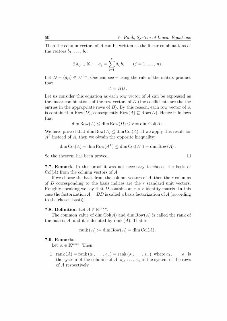
Then the column vectors of A can be written as the linear combinations ofthe vectors b1, . . . , br:

∃ dij ∈ K : aj =r∑

i=1

dijbi (j = 1, . . . , n) .

Let D = (dij) ∈ Kr×n. One can see – using the rule of the matrix productthat

A = BD .

Let us consider this equation as each row vector of A can be expressed asthe linear combinations of the row vectors of D (the coefficients are the theentries in the appropriate rows of B). By this reason, each row vector of Ais contained in Row(D), consequently Row(A) ⊆ Row(D). Hence it followsthat

dimRow(A) ≤ dimRow(D) ≤ r = dimCol(A) .

We have proved that dimRow(A) ≤ dimCol(A). If we apply this result forAT instead of A, then we obtain the opposite inequality:

dimCol(A) = dimRow(AT ) ≤ dimCol(AT ) = dimRow(A) .

So the theorem has been proved. �

7.7. Remark. In this proof it was not necessary to choose the basis ofCol(A) from the column vectors of A.

If we choose the basis from the column vectors of A, then the r columnsof D corresponding to the basis indices are the r standard unit vectors.Roughly speaking we say that D contains an r × r identity matrix. In thiscase the factorization A = BD is called a basis factorization of A (accordingto the chosen basis).

7.8. Definition Let A ∈ Km×n.The common value of dimCol(A) and dimRow(A) is called the rank of

the matrix A, and it is denoted by rank (A). That is

rank (A) := dimRow(A) = dimCol(A) .

7.9. Remarks.Let A ∈ Km×n. Then

1. rank (A) = rank (a1, . . . , an) = rank (s1, . . . , sm), where a1, . . . , an isthe system of the columns of A, s1, . . . , sm is the system of the rowsof A respectively.

7.1. Theory 61

2. rank (A) = rank (AT ).

3. 0 ≤ rank (A) ≤ min{m,n},rank (A) = 0 ⇐⇒ A = 0.

4. rank (A) = m if and only if the row vectors of A are linearly indepen-dent.

rank (A) = n if and only if the column vectors of A are linearly inde-pendent.

7.1.3. System of Linear Equations (Linear Systems)

7.10. Definition Letm ∈ N+ and n ∈ N+ be positive integers. The generalform of the m×n system of linear equations (or: linear equation system, orsimply: linear system) is:

a11x1 + . . . + a1nxn = b1a21x1 + . . . + a2nxn = b2

......

...am1x1 + . . . + amnxn = bm

,

where the coefficients aij ∈ K and the right-side constants bi are given. Thisform is called the scalar form of the linear system.

We are looking for all the possible values of the unknowns (or: variables)x1, . . . , xn ∈ K such that all the equations will be true. Such a systemx1, . . . , xn of values of the variables is called a solution of the linear system.

7.11. Definition The linear system is named consistent if it has a solution.It is named inconsistent if it has no solution.

Let us introduce the vectors

a1 :=

a11a21...

am1

, . . . , an :=

a1na2n...

amn

, b :=

b1b2...bm

in Km. Using them the linear system can be written in the following simplerform:

x1a1 + x2a2 + · · ·+ xnan = b . (7.1)


This form is called the vector form of the linear system. Now we reformu-late the question in the following way: can we expand vector b as a linearcombination of the vectors a1, . . . , an? If yes, then compute the coefficientsof all the possible expansions.

Finally, if we introduce the matrix

A := [a1 . . . an] :=

a11 a12 . . . a1na21 a22 . . . a2n...

......

am1 am2 . . . amn

∈ Km×n ,

which is called the coefficient matrix or simply the matrix of the system,and the unknown vector x := (x1, . . . , xn) ∈ Kn, then the shortest form ofthe linear system is

Ax = b . (7.2)

This is called the matrix form of the linear system.

In this form the problem is to find all the possible vectors x in Kn forwhich the statement Ax = b will be true. Such a vector (if it exists) is calleda solution vector of the system.

7.12. Remark. It is easy to observe that

the system is consistent ⇐⇒ b ∈ Span (a1, . . . , an) = Col(A) .

Thus the consistence of a linear system is equivalent with the question thatb lies in the column space of A or not. Consequently the smaller the columnspace is, the greater is the chance of inconsistence. If rank (A) equals thenumber of rows m (in other words: the rows of A are linearly independent),then Col(A) is the possible greatest subspace that is Col(A) = Km. In thiscase the system is surely consistent.

Let us denote by M the set of the solution vectors of the system Ax = b:

M := {x ∈ Kn | Ax = b} ⊆ Kn .

It is called solution set.

7.13. Definition Two liner systems are said to be equivalent, if their so-lution sets are the same.

7.1. Theory 63

7.14. Remark. The following statements can be considered easily:

1. The linear system can be solved (is consistent) if and only if M = ∅.

2. The solution set of the linear system equals the intersection of thesolution sets of the equations contained in the system.

3. If the linear system contains at least one equation of the form

0x1 + 0x2 + . . . + 0xn = q (q = 0) ,

then the system is inconsistent (it has no solution).

4. The following transformations result equivalent linear systems:

(a) We multiply an equation by a nonzero constant.

(b) We add the constant multiple of an equation to another equation.

(c) We omit an equation of the form

0x1 + 0x2 + . . . + 0xn = 0

from the system.

7.15. Definition Let A ∈ Km×n. The linear system Ax = 0 is called ho-mogeneous system. We often say that Ax = 0 is the homogeneous systemassociated with Ax = b .

Notice, that the homogeneous system is always solvable, because thezero vector is surely a solution of it.

7.16. Theorem Let Mh be the solution set of the homogeneous system,that is

Mh := {x ∈ Kn | Ax = 0} ⊆ Kn .

Then Mh is a subspace in Kn.

Proof. Since 0 ∈ Mh, then Mh = ∅.

Mh is closed under addition, because if x, y ∈ Mh, then Ax = Ay = 0,consequently

A(x+ y) = Ax+ Ay = 0 + 0 = 0 .


Hence it follows that x+ y ∈ Mh.

Furthermore Mh is closed under scalar multiplication too, because ifx ∈ Mh and λ ∈ K, then Ax = 0, consequently

A(λx) = λAx = λ0 = 0 .

Hence it follows that λx ∈ Mh. �

7.17. Definition Let A ∈ Km×n. The subspace Mh is called the null spaceor the kernel space or simply the kernel of matrix A. Its notation is Ker (A).So

Ker (A) := Mh = {x ∈ Kn | Ax = 0} ⊆ Kn .

We now move on to the investigation of the solution sets of consistentlinear systems.

7.18. Theorem (Basic Theorem of Linear Systems)Let A ∈ Km×n, r = rank (A) ≥ 1 (that is A = 0), b ∈ Km, and let us

consider the consistent linear system

Ax = b .

Let

A = [a1 . . . an] , ahol aj ∈ Km .

be the column-partitioned form of A.We know that the column vectors of A form a generator system in

Col(A), furthermore dimCol(A) = r. By this reason we can choose r vectorsfrom the columns of A, which r vectors form a basis in Col(A). Suppose forsimplicity that these r vectors are a1, . . . , ar, the first r columns of A.

Let the unique expansion of b on this basis be

b =r∑

i=1

ciai .

Then

7.1. Theory 65

a) in the case r = n the linear system has the unique solution:

xi = ci (i = 1, . . . , r = n) .

b) in the case 1 ≤ r < n let us consider the unique expansions of thecolumn vectors ar+1, . . . , an ∈ Col(A) relative to the basis a1, . . . , ar:

aj =r∑

i=1

dijai (j = r + 1, . . . , n) .

Then all the solutions of the linear system are:

xi = ci −n∑

j=r+1

dijxj (i = 1, . . . , r) , xr+1, . . . , xn ,

where xr+1, . . . , xn ∈ K are arbitrary numbers. The above formula gives thegeneral solution of the system.

Proof. a) Case r = n

It is trivial by the independence of the vectors a1, . . . , an and by thetheorem of the unique expansion.

b) Case 1 ≤ r < n

We arrive to the general solution by the following equivalent transfor-mations:

Ax = bn∑

i=1

xiai = b

r∑i=1

xiai +n∑

j=r+1

xjaj = b

we substitute b and aj with their expansions:

r∑i=1

xiai +n∑

j=r+1

xj ·r∑

i=1

dijai =r∑

i=1

ciai

We interchange the order of summations, then we rearrange the equations:


r∑i=1

(xi +

n∑j=r+1

dijxj

)· ai =

r∑i=1

ciai

using the independence of the vectors ai and the theorem of unique expan-sion we have

xi +n∑

j=r+1

dijxj = ci (i = 1, . . . , r)

xi = ci −n∑

j=r+1

dijxj (i = 1, . . . , r) .

�

7.19. Remarks.

1. If we agree that the value of the empty sum equals 0, then the casesr = n and r < n can be uniformly summarized in the formula

xi = ci −n∑

j=r+1

xjdij (i = 1, . . . , r), xr+1, . . . , xn ∈ K . (7.3)

2. The variables xr+1, . . . , xn are called free variables, they have arbi-trary values. The variables x1, . . . , xr are called bound variables. Theyare uniquely depending on the free variables. The number n−r is calledthe degree of freedom of the linear system. It gives the number of thefree variables.

3. One can see, that in the case r = n the degree of freedom is 0, thereis no free variable, all the variables are bound variables, the solutionis unique. In the case r < n we have infinitely many solutions withn− r free variables.

4. If we choose in Col(A) another basis instead of the first r columns,then we obtain a similar theorem, only the indexing will be morecomplicated.

Now we will arrange the solutions into a vector, thus we will arrive tothe vector form of the solutions.

7.1. Theory 67

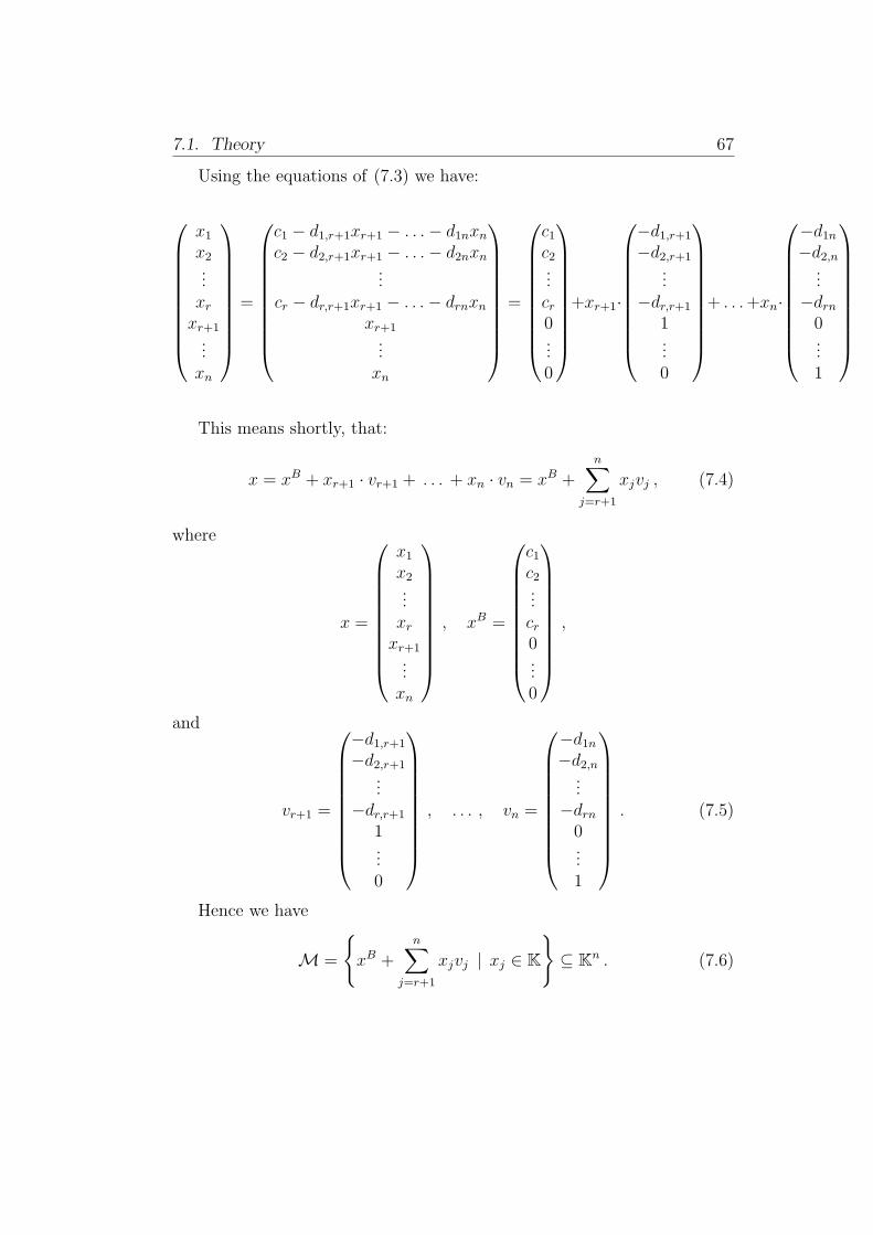
Using the equations of (7.3) we have:

x1

x2...xr

xr+1...xn

=

c1 − d1,r+1xr+1 − . . .− d1nxn

c2 − d2,r+1xr+1 − . . .− d2nxn...

cr − dr,r+1xr+1 − . . .− drnxn

xr+1...xn

=

c1c2...cr0...0

+xr+1·

−d1,r+1

−d2,r+1...

−dr,r+1

1...0

+ . . .+xn·

−d1n−d2,n

...−drn0...1

This means shortly, that:

x = xB + xr+1 · vr+1 + . . . + xn · vn = xB +n∑

j=r+1

xjvj , (7.4)

where

x =

x1

x2...xr

xr+1...xn

, xB =

c1c2...cr0...0

,

and

vr+1 =

−d1,r+1

−d2,r+1...

−dr,r+1

1...0

, . . . , vn =

−d1n−d2,n

...−drn0...1

. (7.5)

Hence we have

M =

{xB +

n∑j=r+1

xjvj | xj ∈ K

}⊆ Kn . (7.6)


7.20. Remark. One can see, that xB is a solution of the linear system,moreover, in the case r = n this is the unique solution.

The following theorem gives the structure of the solution set:

7.21. Theorem (The structure of the solution set)Under the assumptions of theorem 7.18 we have

1. The solution set Mh of the homogeneous system Ax = 0 is an n − rdimensional subspace in Kn. A basis of this subspace is the vectorsystem vr+1, . . . , vn given by the formulas (7.5).

2. If the system Ax = b is consistent (solvable), then its solution set Mis a shifting of the subspace Mh with the vector xB.

Proof.

1. Since the system is homogeneous, then b = 0. Consequently c1 =. . . = cr = 0, that is xB = 0. Let us substitute this into formula (7.6):

Mh =

{n∑

j=r+1

xjvj | xj ∈ K

}.

– In the case r = n it means, that Mh = {0} (the case of the emptysum). Consequently dimMh = 0 = n− n = n− r.

– In the case r < n it means, that vr+1, . . . , vn is a generator system inthe subspace Mh. On the other hand – by the 0 – 1 components – thevectors vr+1, . . . , vn are linearly independent. Thus the vector systemvr+1, . . . , vn is a basis in the subspace Mh, consequently dimMh =n− r.

2. It follows immediately from formula (7.6).

�

7.22. Remarks.

1. In the case r = n the sums in the formulas of M and Mh are empty,consequently we have

Mh = {0}, dimMh = 0, M = {xB} .

7.1. Theory 69

2. Using Ker (A) = Mh and dimMh = n − r and dimCol(A) = r, wehave the following important equality:

dimKer (A) + dimCol(A) = n .

Our theory from above cannot be used to solve a linear system in prac-tice, because it didn’t give an algorithm

– to decide the solvability (consistence) of the linear system,– to determine a basis in Col(A),– to determine the numbers ci and dij.

We will deal with the practical solution in the following section.

7.1.4. Solving a Linear System in Practice

In the secondary school we have learnt two methods for solving systemsof linear equations: the method of substitution and the method of equalcoefficients.

The essentiality of the substitution method is the following:

1. From one of the equations we express one of the unknowns. We markthe equality of expression (for example we frame it).

2. The expression resulting for this unknown we substitute into all theother equations. Thus we get a system involving one less equationsand one less unknowns.

3. We repeat this process until it is possible.

4. After the process has stopped, first we find out whether the systemhas solution or not. If it has, then – using the marked equalities – wedetermine the values of the unknowns.

The essential step of the method of equal coefficients is as follows:

1. Choose two equations from the system in which the coefficients of thesame unknowns are equal. If there are no such equations, then – bymultiplying both sides of the chosen two equations – achieve that thecoefficients of one of the unknowns to be equal.


2. Subtract this two equations from each other. Then the above men-tioned unknown falls out in the resulted equation.

3. We replace one of the originally chosen equations by the resulted equa-tion. The new system will be equivalent with the original one. But oneof its equation surely does not contain the above mentioned unknown.

We can see that the essential step of the method of equal coefficients canbe performed by the method of substitution too: let us express an unknownfrom one of the chosen two equations, and let us substitute it into anotherone. We illustrate this in the following example:

Suppose that the chosen two equations are:

5x1 − 3x2 + 2x3 = 75x1 + x2 + x3 = 3

Let us subtract the second equation from the first one (method of equalcoefficients):

−4x2 + x3 = 4 .

If we apply the substitution method, then let us express x1 from the firstequation:

x1 =3x2 − 2x3 + 7

5,

then let us substitute it into the second equation:

5 · 3x2 − 2x3 + 7

5+ x2 + x3 = 3

4x2 − x3 = −4

−4x2 + x3 = 4 .

We can see, that we have obtained the same equation like at the method ofequal coefficients.

The essential step of the method of equal coefficients can be regardedas we have added a constant multiple of an equation to another one. Thuswe have reached, that an unknown variable has vanished from the equation.If we improve this idea in the way that we add the appropriate constantmultiples of a fixed equation to all the other equations, then we can remove(in Latin terminology: eliminate) an unknown variable from all, but oneequation. This is the base of the elimination methods will be studied in thesubject

”Numerical Methods”.

In our subject Basic Mathematics we will investigate only one version,the Gauss-Jordan elimination method.

7.1. Theory 71

The first important remark is that instead of writing a complete linearsystem we will write only its coefficients and its right-hand side constantterms in a table in the following way:

a11x1 + . . . + a1nxn = b1a21x1 + . . . + a2nxn = b2

......

...am1x1 + . . . + amnxn = bm

⇐⇒

a11 a12 . . . a1n b1a21 a22 . . . a2n b2...

......

...am1 am2 . . . amn bm

.

If an unknown is absent from an equation, then the entry in the tableequals 0, according to the term 0xj. This table is called the augmentedmatrix of the linear system.

One can easily see, that the representation by the augmented matrixrequires less writing. The equations are identified by the rows, the unknownsare identified by the columns to the left of the vertical line, the right-hand-side constants are identified by the column to the right of the vertical line.

The linear system and the augmented matrix can be generated from eachother easily. The operations with the equations correspond to the operationswith the rows of the augmented matrix.


Suppose that the coefficient matrix of the linear system is not the zeromatrix (in the opposite case the system can be discussed easily). The essen-tiality of the Gauss-Jordan method is the iterative repetition of the followingsteps, and after the process has stopped, reading the results out of the lasttable.

1. We choose to the left of the vertical line a nonzero element, which is neither ina marked row nor in a marked column (at the start of the process there is nomarked row and there is no marked column). The chosen element will be namedpivot element. Its row will be the pivot row, its column will be the pivot column, theunknown according to the pivot column will be the pivot unknown (pivot variable).If we cannot choose pivot element, then the process stops.

2. We divide the pivot row by the pivot element. We mark the 1 in the place of thepivot element (it becomes to a marked element).

3. We subtract from each rows except the pivot row the scalar multiple of the pivotrow such that the element of this row in the pivot column becomes 0 (we reset theentries in the pivot column, except the pivot entry). Thus we have reached thatthe pivot column contains a marked 1, and all its other elements are 0-s. The shortname of this step will be

”the zeroing of the pivot column”.

This means in connection with the linear system that we have eliminated an un-known from the equations according to the non-pivot rows, but we have left thisunknown with coefficient 1 in the equation according to the pivot row.

4. We change the attributes”pivot” (element, row, column, unknown) into

”marked”,

then we go to point 1.

The above process is still continued until it terminates by the stoppingcriterion in point 1., that is, until we find pivot element. The process is ob-viously finite, because the number of the marked elements (but the numberof the marked rows and of columns) increases by 1 in every cycle.

Suppose at the termination the number of the marked elements is r.Then the numbers of the marked rows, columns and unknowns are alsor respectively. Remember, that a marked row is a row which contains amarked element, and a marked column is a column which contains a markedelement.

After the termination of the process we consider two cases:

7.1. Theory 73

Case 1., if r = m: In this case each row contains a marked element, thatis each row is a marked row. By this reason, no more pivot element can bechosen. In this case we call the last table reduced table.

Case 2., if r < m: In this case there exist non-marked rows, but it standsonly 0 elements in any non-marked row to the left of the vertical line. Thisis the reason, that we cannot choose a pivot element.

In this case the equation according to a non-marked row looks like:

0x1 + 0x2 + . . . + 0xn = q .

It is obvious that this equation has no solution if q = 0 (prohibited row),consequently the linear system also does not have solution. In the case q = 0any vector x ∈ Kn is a solution of the equation, consequently the equationcan be omitted from the system.

By this reason in the case r < m we have:

- If there is a non-marked row whose last element (that is the elementto the right of the vertical line) is nonzero (prohibited row), thenthe linear system is unsolvable (inconsistent). No reduced table isproduced.

- If the last element (that is the element to the right of the vertical line)of each non-marked row is 0, then we omit the non-marked rows, andthe remainder table will be called the reduced table.

We will show, that if the reduced table exists (as we have seen, it ispossible in two ways), then the linear system is solvable (consistent).

The reduced table has the following properties:

1. It has r rows, and each of its rows is a marked row. This means thateach of its rows has marked element, and we know that this markedelement equals 1.

2. n columns stand to the left of the vertical line, and there are exactly rmarked columns between them. Furthermore, these r marked columnsare exactly the r r-dimensional standard unit vectors. 1 column standsto the right of the vertical line.

3. Hence it follows that in each row stands exactly 1 of the marked un-knowns. The coefficient of this marked unknown is 1, and this markedunknown does not occur in another row. The r marked unknowns areseparated in the r equations.


Finally, we express from each equation the single marked unknown withthe help of the right-side constants and – if it exists – with the help of thenon-marked unknowns. This is very simple, because

– in the case r = n the value of the marked unknown is the right-sideconstant, so one can simply read out it from the table.

– in the case r < n the terms containing non-marked unknowns must beput into the right side.

So, it can be seen, that if the reduced table exists, then the linear systemhas a solution. The solution is unique in the case when r = n, and thereare infinitely many solutions with n − r free parameters in the case whenr < n.

It can be proved (see e.g.: Istvan Csorgo: Linear algebra lecture schemes(2016) Lessons 7 and 8 about the Elementary Basis Transformation), thatthe Gauss-Jordan-method and the Elementary Basis Transformation Methodare the same. Thus we have:

1. The rank of the coefficient matrix is r. Consequently, the number rdetermined in the Gauss-Jordan method is independent of choosingthe pivot elements.

2. The degree of the freedom of the linear system is n− r.

3. The bound variables are identical with the marked variables (un-knowns).

4. The free variables are identical with the non-marked unknowns. Ifthere is no non-marked unknown, then there is no free variable.

5. The numbers ci can be read out from the column to the right of thevertical line in the reduced table.

6. The numbers dij can be read out from the area to the left of thevertical line in the reduced table.

7.23. Remarks.

1. If the system is homogeneous, then in addition to the above, it is alsotrue that the column to the right of the vertical line contains only 0-sin each table. By this reason, the reduced table exists, and its lastcolumn (the column to the right of the vertical line) is identically 0.

7.1. Theory 75

2. The Gauss-Jordan elimination method can be used also to determinethe rank of a matrix. Then we copy the matrix A in the startingtable, there is no vertical line, and there is no column to the right ofthe vertical line. We perform the elimination steps (repetitions of thesteps 1-2-3-4 until it is possible). The rank of the matrix A will be thenumber of the marked elements: rank (A) = r.

7.1.5. Three Computed Examples

In this section we will exemplify the Gauss-Jordan method and its applica-tions via 3 computed examples. In all of the 3 examples the questions areas follows:

a) Determine the size, the coefficient matrix and the right-hand side vec-tor of the linear system.

b) Solve the linear system using the Gauss-Jordan method (solvability,solutions, bound and free variables).

c) The rank of the coefficient matrix.

d) The vector form of the solution (if the system is solvable).

e) The solution set M (if the system is solvable).

f) Solve the corresponding homogeneous system (solutions, solution setMh = Ker (A), basis and dimension of Mh).

In the process of the Gauss-Jordan elimination method the pivot ele-ments will be denoted by framing, the marked elements will be denoted byunderlining.

Example 1 (the case of unique solution)

x2 − 3x3 = −54x1 + 5x2 − 2x3 = 102x1 + 3x2 − x3 = 7


Solution

a)

Obviously m = 3, n = 3, that is the size of the system is 3 × 3. Itscoefficient matrix and right-hand side vector are:

A =

0 1 −34 5 −22 3 −1

∈ R3×3 , b =

−5107

∈ R3 .

b)

Let us write the table (augmented matrix) corresponding to the originallinear system. In step 1. let us choose the second entry of the first row aspivot element. Thus the first row will be the pivot row, the second columnwill be the pivot column, the unknown x2 will be the pivot variable.

0 1 −3 −54 5 −2 102 3 −1 7

.

Now it follows step 2. First we divide the pivot row (it is row 1) by thepivot element (it is 1), then we mark the 1 in the place of pivot element.

Then it follows step 3., the zeroing of the pivot column. First we subtract5

1= 5-times the first row from the second row, then we subtract

3

1= 3-times

the first row from the third row. The result is

0 1 −3 −54 0 13 352 0 8 22

.

In step 4. the first row will be marked, the second column will be marked,the unknown x2 will be marked.

The first cycle is complete.Now it follows again step 1. Let us choose a pivot element (we can choose

between the 4, 13, 2, 8), let it be the first element of the third row:

0 1 −3 −54 0 13 352 0 8 22

.

Thus the third row is the pivot row, the first column is the pivot column,then unknown x1 is the pivot variable.

7.1. Theory 77

It follows step 2., we divide the pivot row (row 3) by the pivot element(by 2), and we mark the 1 in the position of the pivot element. Thus wehave already two marked elements.

After this it follows step 3., the zeroing of the pivot column. First we

subtract0

2= 0-times the third row from the first row, then we subtract

4

2= 2-times the third row from the second row. The result is

0 1 −3 −50 0 −3 −91 0 4 11

.

By step 4. the third row will be marked, the first column will be marked,the unknown x1 will be marked. Now we have two marked elements, twomarked rows, two marked columns, and two marked unknowns.

The second cycle is complete.Now it follows again step 1. Let us choose a pivot element (we can choose

only the −3):

0 1 −3 −50 0 −3 −91 0 4 11

.

Thus the second row is the pivot row, the third column is the pivotcolumn, then unknown x3 is the pivot variable.

It follows step 2., we divide the pivot row (row 2) by the pivot element(by −3), and we mark the 1 in the position of the pivot element. Thus wehave already three marked elements.

After this it follows step 3., the zeroing of the pivot column. First we

subtract−3

−3= 1-times the second row from the first row, then we subtract

4

−3= −4

3-times the second row from the third row. The result is

0 1 0 40 0 1 31 0 0 −1

.

By step 4. the second row will be marked, the third column will bemarked, the unknown x3 will be marked. Now we have three marked ele-ments, three marked rows, three marked columns, and three marked un-knowns.

The third cycle is complete.


Now it follows again step 1. Let us choose a pivot element. We experiencethat all the rows are marked, it is impossible to choose a pivot element. Theelimination process has stopped (it is terminated). We have three markedunknowns, consequently r = 3.

Since all the rows are marked (case r = m), then the system is solvable(consistent), and the reduced table is identical with the last table:

0 1 0 40 0 1 31 0 0 −1

.

Now, let us compute the solutions. Since all the columns are marked(case r = n), then we have a unique solution, which can be read out fromthe last table in the following way:

By the first row we have: x2 = 4.By the second row we have: x3 = 3.By the third row we have: x1 = −1.We see, that if we move from top to bottom, then we obtain the values

of the unknowns not in the natural order x1, x2, x3. If we want to read outthe values of the unknowns in natural order, then we have to rearrange therows of the reduced table such that the part left to the vertical line will bethe identity matrix:

1 0 0 −10 1 0 40 0 1 3

.

7.1. Theory 79

If we disregard the explanations, the Gauss-Jordan elimination methodmeans now the following sequence of tables:

0 1 −3 −54 5 −2 102 3 −1 7

0 1 −3 −54 0 13 352 0 8 22

0 1 −3 −50 0 −3 −91 0 4 11

0 1 0 40 0 1 31 0 0 −1

1 0 0 −10 1 0 40 0 1 3

.

The three marked unknowns x1, x2, x3 are the bound variables. Thereis no free variable.

7.24. Remark. As it is clear from the example, we have to divide by thepivot element. By this reason if we compute on a paper, then we try tochoose as pivot elements 1 or −1, to avoid fractions.

c)

We have three bound variables, thus the rank of the coefficient matrixis rank (A) = 3.

d)


We havex1 = −1; x2 = 4; x3 = 3 .

Let us arrange them into a vector. So we have the vector form solution:

x = (x1, x2, x3) = (−1, 4, 3) .

e)

The solution set of the linear system is a one-element-set:

M = {(−1, 4, 3)} ⊂ R3 .

f)

The unique solution of the homogeneous system is:

x1 = 0; x2 = 0; x3 = 0 , in vector form: x = (0, 0, 0) ∈ R3 ,

its solution set is:

Mh = {(0, 0, 0)} = Ker (A) ⊂ R3 .

This subspace has no basis, its dimension is dimMh = 0, that is identicalwith the number of free variables.

Example 2 (the case of infinitely many solutions)

−3x1 + x2 + x3 − x4 − 2x5 = 22x1 − x2 + x5 = 0−x1 + x2 + 2x3 + x4 − x5 = 8

x2 + x3 + 2x4 = 6

Solution

a)

Obviously m = 4, n = 5, the size of our system is 4 × 5. Its coefficientmatrix and its right-hand-side vector are:

A =

−3 1 1 −1 −22 −1 0 0 1−1 1 2 1 −10 1 1 2 0

∈ R4×5 , b =

2086

∈ R4 .

7.1. Theory 81

b)

(The explanations are on the lectures, or you can apply the explanationsof the first example.)

−3 1 1 −1 −2 22 −1 0 0 1 0−1 1 2 1 −1 80 1 1 2 0 6

−3 1 1 −1 −2 22 −1 0 0 1 05 −1 0 3 3 43 0 0 3 2 4

1 −1 1 −1 0 22 −1 0 0 1 0−1 2 0 3 0 4−1 2 0 3 0 4

0 1 1 2 0 60 3 0 6 1 81 −2 0 −3 0 −40 0 0 0 0 0

.

Now it follows again step 1, choosing a pivot element. We can see thatalthough there is non-marked row, in each non-marked row we have 0-s tothe left of the vertical line. By this reason, it is impossible to choose a pivotelement. The elimination process has stopped (it is terminated). We havethree marked unknowns, consequently r = 3.

Since the last elements of the non-marked rows are 0-s (only the fourthrow is non-marked), then the system is solvable (consistent). The reducedtable can be obtained by cleaning the fourth row:

0 1 1 2 0 60 3 0 6 1 81 −2 0 −3 0 −4

.

Now let us write the solution from the reduced table, by rearrangement:


By the first row we have: x3 = 6− x2 − 2x4.By the second row we have: x5 = 8− 3x2 − 6x4.By the third row we have: x1 = −4 + 2x2 + 3x4.Thus the general solution of the linear system is:

x2 ∈ R, x4 ∈ R, x1 = −4+2x2+3x4, x3 = 6−x2−2x4, x5 = 8−3x2−6x4 .

The three marked unknowns x1, x3, x5 are the bound variables. The twonon-marked unknowns x2, x4 are the free variables.

c)

Since we have three bound variables, then the rank of the coefficientmatrix is rank (A) = 3.

d)

We have

x1 = −4+2x2+3x4; x5 = 8−3x2−6x4; x3 = 6−x2−2x4 (x2, x4 ∈ R) .

Let us arrange them into a vector, and apply the separation technique.So we have the vector form solution:

x =

x1

x2

x3

x4

x5

=

−4 + 2x2 + 3x4

x2

6− x2 − 2x4

x4

8− 3x2 − 6x4

=

−40608

+ x2 ·

21−10−3

+ x4 ·

30−21−6

.

It can be read out that:

xB = (−4, 0, 6, 0, 8), v2 = (2, 1,−1, 0,−3), v4 = (3, 0,−2, 1,−6) .

e)

The solution set of the linear system is an infinite set:

M = {xB + x2v2 + x4v4 | x2, x4 ∈ R} .

f)

7.1. Theory 83

The general solution of the homogeneous system is (consider 0-s to theright of the vertical line in the reduced table):

x2 ∈ R, x4 ∈ R, x1 = 2x2 + 3x4, x3 = x2 − 2x4, x5 = 3x2 − 6x4 .

In vector form it is:

x =

x1

x2

x3

x4

x5

=

2x2 + 3x4

x2

−x2 − 2x4

x4

−3x2 − 6x4

= x2 ·

21−10−3

+ x4 ·

30−21−6

= x2v2 + x4v4 .

the solution set is:

Mh = {x2v2 + x4v4 | x2, x4 ∈ R} = Span (v2, v4) = Ker (A) .

A basis of Mh is: v1, v2. Furthermore dimMh = 2.

Example 3 (the inconsistent case)

2x1 + 3x2 − x3 + 2x4 = −1x1 + 4x2 − 4x3 + 3x4 = 24x1 + x2 + 5x3 = 1

Solution

a)

Obviously m = 3, n = 4, that is the size of the system is 3 × 4. Itscoefficient matrix and right-hand side vector are:

A =

2 3 −1 21 4 −4 34 1 5 0

∈ R3×4 , b =

−121

∈ R3 .

b)

(The explanations are on the lectures, or you can apply the explanationsof the first example.)


2 3 −1 2 −11 4 −4 3 24 1 5 0 1

−10 0 −16 2 −4−15 0 −24 3 −24 1 5 0 1

−5 0 −8 1 −20 0 0 0 44 1 5 0 1

Now it follows again step 1, choosing a pivot element. We can see thatalthough there is non-marked row, in each non-marked row stand 0-s to theleft of the vertical line. By this reason, it is impossible to choose a pivotelement. The elimination process has stopped (it is terminated). We havetwo marked unknowns, consequently r = 2.

Since we have such a non-marked row whose last element is nonzero (row2, it is a prohibited row), then the linear system is unsolvable (inconsistent,antinomic).

c)

We have two marked unknowns, consequently rank (A) = 2.

d)

There is no solution, consequently the vector form solution also does notexist.

e)

The solution set is the empty set: M = ∅.

f)

The general solution of the homogeneous system is (consider 0-s to theright of the vertical line in the reduced table):

x1 ∈ R, x3 ∈ R, x2 = −4x1 − 5x3, x4 = 5x1 + 8x3 .

The two marked unknowns x2, x4 are the bound variables, and the twonon-marked unknowns x1, x3 are the free variables.

7.1. Theory 85

The vector form of the solution of the homogeneous system is:

x =

x1

x2

x3

x4

=

x1

−4x1 − 5x3

x3

5x1 + 8x3

= x1 ·

1−405

+ x3 ·

0−518

.

The solution set of the homogeneous system is:

Mh = {x1v1 + x3v3 | x1, x3 ∈ R} = Span (v1, v3) = Ker (A) .

A basis of Mh is: v1 = (1,−4, 0, 5), v3 = (0,−5, 1, 8) . FurthermoredimMh = 2.


1. Define the rank of a vector system.

2. State the theorem about the connection between the dimensions ofthe row space and of the column space.

3. Define the rank of a matrix.

4. Write the scalar form and the vector form of a linear system.

5. Define the following sets: M, Mh, Ker (A).

6. State the theorem about the structure of the solution set of the ho-mogeneous linear system.

7. State the theorem about the structure of the solution set of the generallinear system.


7.2. Exercises


1. Consider the following systems of linear equations:

(a)x2 − 3x3 = −5

4x1 + 5x2 − 2x3 = 102x1 + 3x2 − x3 = 7

(b)−3x1 + x2 + x3 − x4 − 2x5 = 22x1 − x2 + x5 = 0−x1 + x2 + 2x3 + x4 − x5 = 8

x2 + x3 + 2x4 = 6

(c)2x1 + 3x2 − x3 + 2x4 = −1x1 + 4x2 − 4x3 + 3x4 = 24x1 + x2 + 5x3 = 1

Answer the following questions for each of them:

a) Give the size, the coefficient matrix and its size, and also theright hand side vector b of the system.

b) Solve the system of linear equations (it is consistent or not, findall solutions, give the solutions in scalar form, bound variables,free variables).

c) Find the rank of the coefficient matrix.

d) If the system is consistent, give the vector form of the solutionstoo.

e) If the system is consistent, give the solution set M.

f) Give the solution set (Mh = Ker (A)) of the associated homoge-neous system. Determine a basis in Mh. Find the dimension ofthe subspace Mh.

2. Let

A =

1 1 3 12 3 1 11 0 8 2

∈ R3×4 .

7.2. Exercises 87

Determine a basis in the subspace

Ker (A) := {x ∈ R4 | Ax = 0} .

Find the dimension of Ker (A).


1. Consider the following systems of linear equations:

a)x1 + 2x2 − 3x3 = 62x1 − x2 + 4x3 = 1x1 − x2 + x3 = 3

b)x1 + x2 + 2x3 = 5x1 + x3 = −22x1 + x2 + 3x3 = 3

Answer the following questions for each of them:

a) Give the size, the coefficient matrix and its size, and also theright hand side vector b of the system.

b) Solve the system of linear equations (it is consistent or not, findall solutions, give the solutions in scalar form, bound variables,free variables).

c) Find the rank of the coefficient matrix.

d) If the system is consistent, give the vector form of the solutionstoo.

e) If the system is consistent, give the solution set M.

f) Give the solution set (Mh = Ker (A)) of the associated homoge-neous system. Determine a basis in Mh. Find the dimension ofthe subspace Mh.

2. Let

A =

3 1 91 2 −22 1 5

.

Determine a basis in the subspace

Ker (A) := {x ∈ R3 | Ax = 0}

Find the dimension of Ker (A).


3. Determine the ranks of the following matrices:

A =

2 0 −14 0 −20 0 0

B =

1 3 −1 −22 4 3 5−1 1 3 4

8. Connection with the InverseMatrix

8.1. Theory

8.1.1. Linear System with Square Matrix

8.1. Theorem (Linear system with square matrix) Consider the lin-ear system Ax = b given by the square matrix A ∈ Kn×n and by the vectorb ∈ Kn. Then

a) In the case rank (A) = n the linear system has a unique solution-b) In the case rank (A) ≤ n− 1 the linear system either has no solution

or the linear system has infinitely many solutions.

Proof.a) Suppose that r = rank (A) = n.

Then the column vectors of A form an n-term linearly independent sys-tem in the n dimensional space Kn. Consequently, they form a basis in Kn,thus Col(A) = Kn. By this reason b ∈ Col(A), that is the linear system hasa solution.

On the other hand, the degree of freedom is n− r = n−n = 0, thus thesolution is unique.

b) Suppose that r = rank (A) ≤ n− 1.In this case by dimCol(A) = r < n = dimKn we have

Col(A) ⊂ Kn Col(A) = Kn .

If so b /∈ Col(A), then the system has no solution. However, if b ∈ Col(A),then the system is solvable, and the degree of freedom is

n− r ≥ n− (n− 1) = 1 ,

consequently the system has infinitely many solutions. �

90 8. Connection with the Inverse Matrix

8.1.2. Inverse Matrix and the Linear System

We can use our results about the linear systems with square matrix also fordetermination of the inverse matrix.

8.2. Theorem Let A ∈ Kn×n be a square matrix. Then

a) rankA = n =⇒ A the matrix A is invertible (regular);b) rankA < n =⇒ A the matrix A is non-invertible (singular).

Proof. Denote by I the n×n identity matrix. Its columns are the standardunit vectors:

I =[e1 e2 . . . en

].

We are looking for the inverse of A, that is, we are looking for the matrix

X =[x1 x2 . . . xn

]∈ Kn×n

such that AX = I is true.

The matrix equation AX = I can be written as follows:

A ·[x1 x2 . . . xn

]=[e1 e2 . . . en

],

Which is equivalent the collection of the following linear systems:

Ax1 = e1, Ax2 = e2, . . . , Axn = en . (8.1)

Now we go to the proofs of the statements a) and b):

a) Since r = n at each linear system, then – using the previous theorem –each linear system can be solved uniquely. It implies, that there exists A−1,and that the columns of A−1 are the solution vectors x1, . . . , xn.

b) Since dimCol(A) = r < n, then all the standard unit vectors e1, . . . , encannot be in Col(A). Thus – using the previous theorem – at least oneof the above collection of linear systems is antinomic, it has no solution.Consequently A−1 does not exist. �

8.3. Remark. It follows from the theorem, that its parts a) and b) areactually equivalences

After all – considering also the connection between the determinants andthe inverses – we can characterize the regular and the singular matrices asfollows:

The 5 characterizations of a regular matrix A ∈ Kn×n:

8.1. Theory 91

1. ∃A−1

2. det(A) = 0

3. rank (A) = n

4. the columns of A are linearly independent

5. the rows of A are linearly independent

The 5 characterizations of a singular matrix A ∈ Kn×n:

1. @A−1

2. det(A) = 0

3. rank (A) < n

4. the columns of A are linearly dependent

5. the rows of A are linearly dependent

8.1.3. Computation of the Inverse Matrix with Gauss-Jordan Method

By the results of the previous section we can establish that to determinethe inverse of an n × n matrix we have to solve n linear systems. Fromthe point of view of the amount of arithmetic operations This method ismore effective than the method of the cofactors (see in the chapter aboutthe determinants). Thus we can compute the inverse matrix solving this nlinear systems after each other.

But the coefficient matrices of these linear systems are the same, sowe obtain a more effective method, if we solve the n linear systems notafter each other, but simultaneously at the same time. The Gauss-Jordanmethod makes it possible. We need only the modification that in the startingtable we put – by (8.1) – the n standard unit vectors, to the right of thevertical line. Then we perform the learnt elimination cycles with this n×2naugmented table.

– If you don’t have the n marked element at the stopping of the elimi-nation cycles, then the matrix is singular, it has no inverse.


– If you have the n marked element at the stopping of the eliminationcycles, then the matrix is regular, it has inverse. To read out the inverse,we have to rearrange the rows of the last table (it is the reduced table atthe same time), such that the block to the left of the vertical line will bethe identity matrix. Then the inverse matrix will be the block to the rightof the vertical line.

The rank of the matrix will be in both cases the number of the markedelements.

Let us look at these two developed examples:

8.1. Theory 93

1. Example Using Gauss-Jordan method determine the inverse of the ma-trix

A =

5 2 −33 1 −22 −3 −4

∈ R3×3 .

Solution

5 2 −3 1 0 03 1 −2 0 1 02 −3 −4 0 0 1

−1 0 1 1 −2 03 1 −2 0 1 011 0 −10 0 3 1

−1 0 1 1 −2 01 1 0 2 −3 01 0 0 10 −17 1

0 0 1 11 −19 10 1 0 −8 14 −11 0 0 10 −17 1

1 0 0 10 −17 10 1 0 −8 14 −10 0 1 11 −19 1

We can read out here that the matrix is regular, its inverse is

A−1 =

10 −17 1−8 14 −111 −19 1

∈ R3×3 .

Since there are three marked elements, the rank of the matrix equals 3.


2. Example Using Gauss-Jordan method determine the inverse of the ma-trix

A =

1 1 −12 0 3−3 1 −7

∈ R3×3 .

Solution

1 1 −1 1 0 02 0 3 0 1 0−3 1 −7 0 0 1

4 0 6 1 0 −12 0 3 0 1 0−3 1 −7 0 0 1

0 0 0 1 −2 −11 0 3/2 0 1/2 00 1 −5/2 0 3/2 1

The elimination process has stopped, because it was impossible to findpivot element. Since the number of the marked elements is less than 3, thenthe matrix is non-invertible, it is singular.

Since there are two marked elements, the rank of the matrix equals 2.

You find an example for the inverse of a 4× 4 matrix in the Appendix.


1. Stte the theorem about the linear systems with square matrices.

2. State the theorem about the connection between the rank and theinvertibility of a matrix.

3. Write the 5 equivalent characterizations of the regular matrices.

4. Write the 5 equivalent characterizations of the singular matrices.

8.2. Exercises 95

8.2. Exercises


1. Solve the following system of linear equations (the exercise was solvedon the previous practice). Is the coefficient matrix regular or singular?Find the rank of the coefficient matrix.

x2 − 3x3 = −54x1 + 5x2 − 2x3 = 102x1 + 3x2 − x3 = 7

2. Using Gauss-Jordan method determine the inverses of the matrices

a) A =

5 2 −33 1 −22 −3 −4

∈ R3×3 b) A =

1 1 −12 0 3−3 1 −7

∈ R3×3

3. Find the rank of the following matrix. Is the coefficient matrix regularor singular?

A =

5 1 −7 −20 2 1 11 5 1 2−3 −1 4 1

∈ R4×4

4. Consider the matrix of the previous exercise:

A =

5 1 −7 −20 2 1 11 5 1 2−3 −1 4 1

∈ R4×4 ,

and letb1 = (−1, 3, 7, 0), b2 = (0, 5, 7,−1) ∈ R4 .

Prove thata) the linear system Ax = b1 has infinitely many solutions,b) the linear system Ay = b2 has no solution.



1. Solve the following system of linear equations. Is the coefficient matrixregular or singular? Find the rank of the coefficient matrix.

a)x1 + 2x2 − 3x3 = 62x1 − x2 + 4x3 = 1x1 − x2 + x3 = 3

b)x1 + x2 + 2x3 = 5x1 + x3 = −22x1 + x2 + 3x3 = 3

2. Using Gauss-Jordan method determine the inverses of the matrices

a) A =

4 3 1−3 −5 −29 4 1

∈ R3×3 b) A =

2 1 43 2 50 −1 1

∈ R3×3

3. Consider the matrix

A =

1 3 4−2 −5 −31 4 9

∈ R3×3 .

(a) Determine its rank. Is the matrix A regular or singular?

(b) Determine the vectors b1, b2 ∈ R3 \ {0} such that the systemAx = b1 is consistent and the system Ax = b2 is inconsistent.

9. Eigenvalues andEigenvectors of MatricesIn this chapter we investigate that in the case of a given matrix A ∈ Kn×n inwhich directions in Kn will be the result of the multiplication by A parallelwith the original direction. These directions (if they exist) will be calledeigen-directions.

The question raised above is in close connection with the linear transfor-mations, therefore let us speak some words about the linear transformations.

9.1. Theory

9.1.1. Linear Transformations in Kn

9.1. Definition A function φ : Kn → Kn is called a linear transformationof the space Kn if

a) φ(x+ y) = φ(x) + φ(y) (x, y ∈ Kn), and

b) φ(λx) = λφ(x) (x ∈ Kn, λ ∈ K).

A linear transformation in R2 is for example the line reflection about thex-axis. Also a linear transformation in R2 is the rotation about the originthrough +90◦.

If A ∈ Kn×n then the function

φ : Kn → Kn, φ(x) = Ax

is a linear transformation in Kn. It can be proved that to each lineartransformation in Kn there exist a unique matrix A ∈ Kn×n such thatφ(x) = Ax (x ∈ Kn). Thus any linear transformation of Kn can be charac-terized by an n× n matrix in Kn×n. This matrix is called the matrix of thelinear transformation.

9.2. Examples

1. The matrix of the above mentioned line reflection about the x-axis is:[1 00 −1

]

98 9. Eigenvalues and Eigenvectors of Matrices

2. The matrix of the above mentioned rotation about the origin through+90◦ is: [

0 −11 0

]An interesting question is, that a linear transformation in which direc-

tions behaves as central dilation, that is for which vectors x ∈ Kn \ {0} andnumbers λ ∈ K holds

φ(x) = λx (the formulation of the eigenvalue problem with transformations) .

Using the matrix of the transformation we have

Ax = λx (the formulation of the eigenvalue problem with matrices) .

We will investigate this last question, in the formulation with matrices.

9.1.2. Basic Concepts

9.3. Definition Let A ∈ Kn×n and λ ∈ K. The number λ is called theeigenvalue of the matrix A if

∃ x ∈ Kn, x = 0 : Ax = λx .

The above vector x ∈ Kn \ {0} is called an eigenvector of A associated withthe eigenvalue λ. The equation Ax = λx is called the eigenvalue-equation.

The set of the eigenvalues is called the spectrum of the matrix A, itsnotation is: Sp (A). So

Sp (A) := {λ ∈ K | ∃x ∈ Kn \ {0} : Ax = λx} ⊆ K .

After a simple rearrangement one can see, that the equation Ax = λxis equivalent with the following homogeneous system of linear equations forany fixed λ ∈ K:

(A− λI)x = 0 , (9.1)

where I denotes the identity matrix in Kn×n.Using the theory of systems of linear equations hence follows that the

number λ ∈ K is an eigenvalue of A if the above system of linear equationshas infinitely many solutions. But this last statement – using the theory ofsquare linear systems – is equivalent with the fact that the determinant ofits coefficient matrix A− λI equals 0. So the parameter λ must satisfy theequation

det(A− λI) = 0 .

9.1. Theory 99

The left-hand side of this equation is a polynomial of the variable λ, becauseat the expansion of the determinant we use only addition and multiplica-tion. The roots in K of this polynomial are the eigenvalues. The eigenvectorsassociated with a fixed eigenvalue are the nontrivial solutions of the homo-geneous system of linear equations (9.1).

9.4. Definition The polynomial

P (λ) = PA(λ) = det(A− λI) =

∣∣∣∣∣∣∣∣∣a11 − λ a12 . . . a1na21 a22 − λ . . . a2n...

......

an1 an2 . . . ann − λ

∣∣∣∣∣∣∣∣∣ (λ ∈ K)

is called the characteristic polynomial of the matrixA. The equation PA(λ) =0 is called characteristic equation.

9.5. Remark. The expansion of the above determinant shows that thecharacteristic polynomial has the degree n, and the coefficient of λn (theleading coefficient) is (−1)n. Moreover – since P (0) = det(A−0I) = det(A)– it follows that its constant term equals det(A). Thus the characteristicpolynomial has the following form:

P (λ) = (−1)n · λn + . . .+ det(A) (λ ∈ K) .

In the”Precalculus” part of the subject

”Basic Mathematics” we have

learnt about the multiplicity of a real root of a polynomial. Similarly we candefine the multiplicity of complex roots. Using this concepts we can give thefollowing definition:

9.6. Definition Let P be the characteristic polynomial of a matrix A ∈Kn×n, and let λ ∈ K be an eigenvalue of A (that is a root of P ). Themultiplicity of the root λ is called the algebraic multiplicity of the eigenvalueλ, and is denoted by a(λ).

Since the eigenvalues are the roots of the characteristic polynomial inK, we can establish that:

• If K = C, then Sp (A) = ∅, and has maximally n elements. If everyeigenvalue is counted as many times as its algebraic multiplicity, thenthe number of eigenvalues is exactly n.


• If K = R, then Sp (A) may be the empty set, and it has maximallyn elements. But even though every eigenvalue is counted as manytimes as its algebraic multiplicity, it is not sure, that the number ofeigenvalues is exactly n. In the case when – counting the eigenvalueswith their algebraic multiplicity – the number of eigenvalues is exactlyn, then we say that all the eigenvalues of the matrix are real.

The eigenvalues of triangular matrices (especially of diagonal matrices)can be obtained easily, as it can be seen in the following remark.

9.7. Remark. Let A ∈ Kn×n be a (lower or upper) triangular matrix.Then – e.g. in the lower triangular case – its characteristic polynomial is asfollows:

P (λ) =

∣∣∣∣∣∣∣∣∣a11 − λ 0 . . . 0a21 a22 − λ . . . 0...

......

an1 an2 . . . ann − λ

∣∣∣∣∣∣∣∣∣ =

= (a11 − λ) · (a22 − λ) · · · · · (ann − λ) (λ ∈ K) .

We have used, that the determinant of a triangular matrix equals the prod-uct of its diagonal entries.

Consequently, the eigenvalues of a triangular matrix are its diagonalentries. The algebraic multiplicity of each eigenvalue is the number of howmany times it occurs in the diagonal.

Let us move on to the investigation of eigenvectors. First we will show,that infinitely many eigenvectors are associated with a fixed eigenvalue.Moreover, these infinitely many eigenvectors and the zero vector togetherform a subspace in Kn.

9.8. Theorem Let A ∈ Kn×n and λ ∈ Sp (A). Then the set

Wλ := Wλ(A) := {x ∈ Kn | Ax = λx}

consisting of the eigenvectors associated with λ and of the zero vector formsan n− rank (A−λI) dimensional subspace in Kn. Infinitely many eigenvec-tors are associated with the eigenvalue λ.

9.1. Theory 101

Proof.

Wλ = {x ∈ Kn | Ax = λx} = {x ∈ Kn | (A− λI)x = 0} = Sh

Using the learned results about the homogeneous linear systems, the aboveset is really a subspace whose dimension is

dimWλ = dimSh = n− rank (A− λI) .

Since dimWλ = n − rank (A − λI) ≥ 1, then the set of the associatedeigenvectors (Wλ \ {0}) is really infinite. �

At a fixed eigenvalue the real question is not the number of the as-sociated eigenvectors, but the maximal number of independent associatedeigenvectors, that is the dimension of the subspace Wλ.

9.9. Definition The subspace

Wλ := Wλ(A) := {x ∈ Kn | Ax = λx}

defined in the above theorem is called the eigenspace corresponding to theeigenvalue λ. The dimension ofWλ is called the geometric multiplicity of theeigenvalue λ. It is denoted by g(λ). Thus we have g(λ) = n− rank (A−λI).

The geometric multiplicity cannot exceed the algebraic one. This is ex-pressed in the following theorem, which is given here without proof.

9.10. Theorem

∀λ ∈ Sp (A) : 1 ≤ g(λ) ≤ a(λ) ≤ n .

9.1.3. Eigenvector Basis (E.B.)

The following theorem will be stated without proof. Essentially it states,that eigenvectors associated with different eigenvalues are linearly indepen-dent.

9.11. Theorem Let A ∈ Kn×n, and λ1, . . . , λk be k different eigenvalues ofmatrix A. Further let si ∈ N+, 1 ≤ si ≤ g(λi), and x

(1)i , x

(2)i , . . . , x

(si)i be a

linearly independent system in the eigenspace Wλi(i = 1, . . . , k). Then the

united vector system

x(j)i ∈ Kn (i = 1, . . . , k; j = 1, . . . , si) (9.2)

is linearly independent.


For each λ ∈ Sp (A) let us take the maximal number (that is g(λ))linearly independent eigenvectors in the eigenspaceWλ. Their united system– in the sense of the above theory – is linearly independent, and the numberof members in the united system equals

∑λ∈Sp (A)

g(λ). Thus we can establish

∑λ∈Sp (A)

g(λ) ≤ n .

In the case when equality holds in the above inequality, we have n inde-pendent vectors in the n dimensional space Kn. Consequently this unitedvector system is a basis in Kn.

9.12. Definition The basis described above is called Eigenvector Basis(E.B.)

We can easily conclude now that

∃ E.B. ⇐⇒∑

λ∈Sp (A)

g(λ) = n .

Using the connection between the algebraic and geometric multiplicities(see theorem 9.10) the following theorem can be proved:

9.13. Theorem Let A ∈ Kn×n, a(λ) be the algebraic multiplicity, and g(λ)be the geometric multiplicity of the eigenvalue λ. Then

∃ E.B. ⇐⇒∑

λ∈Sp (A)

a(λ) = n and ∀λ ∈ Sp (A) : g(λ) = a(λ) .

9.14. Remark. The condition∑

λ∈Sp (A)

a(λ) = n expresses that the charac-

teristic polynomial – counting the roots with their multiplicity – has n rootsin K. This condition

- in case K = C is met”automatically”.

- in case K = R is met if and only if all the roots of the characteristicpolynomial are real.

9.2. Exercises 103


1. Define the eigenvalue and the eigenvector of a matrix

2. Define the characteristic polynomial

3. Define the algebraic multiplicity of an eigenvalue

4. Give the eigenvalues of a triangular matrix

5. Define the eigenspace

6. Define the geometric multiplicity of an eigenvalue

7. What is the connection between the algebraic and the geometric mul-tiplicity of an eigenvalue?

8. State the theorem about the independence of eigenvectors

9. Define the concept of Eigenvector Basis (E. B.)

10. Give the theorems about the necessary and sufficient condition of theexistence of Eigenvector Basis (2 theorems)

9.2. Exercises


1. Determine the eigenvalues and the eigenvectors of the following ma-trices. Determine the eigenspaces, the algebraic and the geometricmultiplicities of the eigenvalues. Is there an eigenvector basis in theadequate vector space?

Solve the above problems in the case K = R and in the case K = Ctoo.

a) A =

2 −1 −13 −2 −3−1 1 2

b) A =

1 −1 11 1 −10 −1 2


c) A =

1 −1 11 1 −12 −1 0

d) A =

1 −1 −11 1 03 0 1


1. Determine the eigenvalues and the eigenvectors of the following ma-trices. Determine the eigenspaces, the algebraic and the geometricmultiplicities of the eigenvalues. Is there an eigenvector basis in theadequate vector space?


a)

[2 −110 −9

]b)

[−2 −71 2

]c)

5 1 30 −1 00 1 2

d) A =

[2 −31 −1

]e)

1 2 −2−3 4 0−3 1 3

10. Diagonalization of Matrices

10.1. Theory

10.1.1. Similarity of Matrices

10.1. Definition Let A,B ∈ Kn×n. We say that matrix B is similar tomatrix A (in notation: A ∼ B), if

∃C ∈ Kn×n : C invertible, and B = C−1AC .

Matrix C is called similarity matrix.

10.2. Remark. The similarity relation is symmetric, that is A ∼ B ⇒B ∼ A. So we can refer to similarity as

”A and B are similar (to each

other)”.

10.3. Theorem If A ∼ B, then PA = PB, that is, their characteristicpolynomials coincide. Consequently their eigenvalues (with algebraic multi-plicities) and their determinants coincide too.

Proof. Let A,B,C ∈ Kn×n, and suppose B = C−1AC. Then for any λ ∈ Kholds

PB(λ) = det(B − λI) = det(C−1AC − λC−1IC) = det(C−1(A− λI)C) =

= det(C−1) · det(A− λI) · det(C) = det(C−1) · det(C) · det(A− λI) =

= det(C−1C) · det(A− λI) = det(I) · PA(λ) = 1 · PA(λ) = PA(λ) .

This exactly means that PA = PB. �

10.1.2. Diagonalizability

In the following definition we define an important class of matrices.

10.4. Definition Let A ∈ Kn×n. We say that A is diagonalizable (some-times the word

”diagonable” is used) over K, if it is similar to a diagonal

matrix, that is, if

∃C ∈ Kn×n, C is invertible : C−1AC is a diagonal matrix .

Matrix C is called diagonalizing similarity matrix, and the diagonal matrixD = C−1AC is called the diagonal form of A.

106 10. Diagonalization of Matrices

10.5. Remark. If A is diagonalizable, then the diagonal entries of its diag-onal form are the eigenvalues of A. Each eigenvalue stands in the diagonalas many times as its algebraic multiplicity is.

The essentiality of the following theorem is that the diagonalizability isequivalent with the existence of the Eigenvector Basis (E.B.)

10.6. Theorem Let A ∈ Kn×n. The matrix A is diagonalizable over K ifand only if there exists E.B. in Kn.

Proof. First suppose that A is diagonalizable. Let c1, . . . , cn ∈ Kn be thecolumn vectors of the diagonalizing similarity matrix C:

C = [c1 . . . cn] .

We will show that c1, . . . , cn is an E.B.By the invertibility of C the n-term system c1, . . . , cn is linearly inde-

pendent, consequently it is a basis in Kn.To prove that the vectors cj are eigenvectors, let us start from equation

C−1AC =

λ1

. . .

λn

,

where λ1, . . . , λn are the eigenvalues of A. Multiply this equation by C fromthe left:

A · [c1 . . . cn] = C ·

λ1

. . .

λn

= [c1 . . . cn] ·

λ1

. . .

λn

[Ac1 . . . Acn] = [λ1c1 . . . λncn]

Using the column-wise equality we have

Acj = λjcj (j = 1, . . . , n)

So the basis really consists of eigenvectors.

Conversely, suppose c1, . . . , cn is an E.B. in Kn. Let C ∈ Kn×n be thematrix built from the columns c1, . . . , cn.

C is obviously invertible, because its columns are linearly independent.

10.1. Theory 107

Let us write the eigenvalue-equations:

Acj = λjcj (j = 1, . . . , n) ,

then perform the steps written in the first half of the proof in the oppositedirection. Then we have the following equality:

C−1AC =

λ1

. . .

λn

.

We can see that A is really diagonalizable. �

10.7. Remarks.

1. One can see that the order of the eigenvector-columns in C is thesame as the order of the corresponding eigenvalues in the diagonal ofC−1AC.

2. If a matrix A ∈ Kn×n has n pairwise distinct eigenvalues in K, thenthe corresponding n eigenvectors are linearly independent. Thus theyform an E.B., consequently A is diagonalizable.

Considering our theorems, we suggest the following algorithm for dis-cussing the diagonalizability of a matrix A ∈ Kn×n:

Step1.:Determine the eigenvalues with their algebraic multiplicities (solvethe characteristic equation).

Step 2.: If the sum of the algebraic multiplicities is less than n, thenstop, the matrix is non-digonalizable. Otherwise go to Step 3.

Step 3.: (The sum of the algebraic multiplicities equals n.) Take aneigenvalue and determine its geometric multiplicity.

Step 3A.: If the geometric multiplicity is less than the algebraic one,then stop, the matrix is non-diagonalizable. Otherwise go to Step 3B.

Step 3B.: If the geometric multiplicity equals the algebraic one, thendetermine the associated eigenvectors.

Repeat this process for all eigenvalues. If you performed Step 3B only,then continue with Step 4.

Step 4.: (The algebraic and the geometric multiplicities are equal forall eigenvalues.) The matrix is diagonalizable. The diagonalizing similaritymatrix and the diagonal form can be obtained by the Remark 10.7.


10.1.3. Two Computed Examples

For illustration of eigenvalues, eigenvectors, diagonalizability let us see twocomputed examples.

In each of the two exercises the questions are as follows:

(a) Determine the eigenvalues, eigenvectors, eigenspaces, algebraic andgeometric multiplicities.

(b) Determine the existence of E.B.

(c) Discuss the diagonalizability of the matrix (diagonalizing similaritymatrix, diagonal form)

Answer these questions in the cases K = R and K = C too.

Example 1

A =

2 −1 −13 −2 −3−1 1 2

∈ K3×3.

SolutionThe characteristic polynomial is

P (λ) = det(A− λI) =

∣∣∣∣∣∣2− λ −1 −13 −2− λ −3−1 1 2− λ

∣∣∣∣∣∣ == (2− λ) · [(−2− λ)(2− λ) + 3] + 1 · [3(2− λ)− 3]− 1 · [3− (2 + λ)] =

= (2− λ)(λ2 − 1)− 2λ+ 2 = (2− λ)(λ+ 1)(λ− 1)− 2(λ− 1) =

= (λ− 1)(λ− λ2) = −λ(λ− 1)2 (λ ∈ K) .

The eigenvalues are the roots of this polynomial:λ1 = 0, its algebraic multiplicity is a(0) = 1, because it is a single root.λ2 = 1, its algebraic multiplicity is a(1) = 2, because it is a double root.So we have

Sp (A) = {0; 1}.

If each eigenvalue is counted by its algebraic multiplicity, then we can alsosay that

λ1 = 0, λ2 = 1, λ3 = 1.

Let us determine the eigenvectors.

10.1. Theory 109

In the case λ1 = 0 the linear system to be solved is 2 −1 −13 −2 −3−1 1 2

·

x1

x2

x3

=

000

.

Its nontrivial solutions are the eigenvectors:

x =

x1

3x1

−x1

= x1 ·

13−1

(x1 ∈ K \ {0}).

The corresponding eigenspace is one dimensional (it is a line), whose basis(direction vector) is the vector (1, 3, −1) . By this reason the geometricmultiplicity of the eigenvalue λ1 = 0 is g(0) = 1.

In the case λ2 = 1 the linear system to be solved is 1 −1 −13 −3 −3−1 1 1

·

x1

x2

x3

=

000

.


x =

x2 + x3

x2

x3

= x2·

110

+x3·

101

(x2, x3 ∈ K, (x2, x3) = (0, 0)).

The corresponding eigenspace is two dimensional (it is a plane), whose basisis the vector system (1, 1, 0), (1, 0, 1). By this reason the geometric multi-plicity of the eigenvalue λ2 = 1 is g(1) = 2.

Now comes the discussion of the diagonalizability:The sum of the algebraic multiplicities of the eigenvalues equals a(1) +

a(0) = 2 + 1 = 3, thus we can go on. The geometric multiplicities areidentical with the algebraic ones:

g(0) = a(0) = 1, g(1) = a(1) = 2.

Therefore the matrix A is diagonalizable over K. Let us note that here wecannot apply the sufficient condition

”A has 3 different eigenvalues”. The

E.B. is the united system of eigenvectors:

c1 = (1, 3,−1), c2 = (1, 1, 0) c3 = (1, 0, 1).


The diagonalizing similarity matrix is built of the vectors of the E.B.

C =

1 1 13 1 0−1 0 1

∈ K3×3.

Finally, the diagonal form of A is (we write the eigenvalues into the diagonal)

C−1AC =

0 0 00 1 00 0 1

∈ K3×3.

Example 2

A =

1 −1 11 1 −10 −1 2

∈ K3×3.

SolutionThe characteristic polynomial (expansion by the first row is suggested) is:

P (λ) = det(A− λI) =

∣∣∣∣∣∣1− λ −1 11 1− λ −10 −1 2− λ

∣∣∣∣∣∣ == (1− λ) · [(1− λ)(2− λ)− 1]− 1 · [(−1)(2− λ) + 1] =

= (1− λ)(λ2 − 3λ+ 1) + 1− λ = (1− λ)(λ2 − 3λ+ 2) =

= (1− λ)(λ− 1)(λ− 2) (λ ∈ K).

Hence the eigenvalues are λ1 = 1, λ2 = 2, their algebraic multiplicities area(1) = 2, a(2) = 1. So we have

Sp (A) = {1; 2}.

If each eigenvalue is counted by its algebraic multiplicity, then we can alsosay that

λ1 = 1, λ2 = 1, λ3 = 2.

Let us determine the eigenvectors.In the case λ1 = 1 the linear system to be solved is0 −1 1

1 0 −10 −1 1

·

x1

x2

x3

=

000

.

10.1. Theory 111


x =

x2

x2

x2

= x2 ·

111

(x2 ∈ K \ {0}).

The corresponding eigenspace is one dimensional (it is a line), whose ba-sis (direction vector) is the vector (1, 1, 1) . By this reason the geometricmultiplicity of the eigenvalue λ1 = 1 is g(1) = 1.

In the case λ2 = 2 the linear system to be solved is−1 −1 11 0 −10 −1 0

·

x1

x2

x3

=

000

.


x =

x1

0x1

= x1 ·

101

(x1 ∈ K \ {0}).

The corresponding eigenspace is one dimensional (it is a line), whose ba-sis (direction vector) is the vector (1, 0, 1). By this reason the geometricmultiplicity of the eigenvalue λ2 = 2 is g(2) = 1.

Now comes the discussion of the diagonalizability:

The sum of the algebraic multiplicities of the eigenvalues equals

a(1) + a(2) = 2 + 1 = 3 ,

thus we can go on. But the identity between the algebraic and the geometricmultiplicities is not true for any eigenvalues, because

g(1) = 1 < a(1) = 2.

Consequently we can establish – without discussing the other eigenvalues –that the matrix A is not diagonalizable over K and the E.B. does not existin Kn neither in case K = R, nor in case K = C.



1. Define the similarity of matrices

2. State and prove the theorem about the characteristic polynomials ofsimilar matrices

3. Define the concept of a diagonalizable matrix

4. What are the diagonal entries of the diagonal form of a diagonalizablematrix?

5. State and prove the necessary and sufficient condition of diagonaliz-ability

10.2. Exercises


1. The eigenvalues and the eigenvectors of the following matrices arediscussed in the previous practice.

(a) Let us quote the results.

(b) Determine whether these matrices are diagonalizable or not. Inthe diagonalizable case determine the matrix C that diagonalizesA and the diagonal form C−1AC.


a) A =

2 −1 −13 −2 −3−1 1 2

b) A =

1 −1 11 1 −10 −1 2

c) A =

1 −1 11 1 −12 −1 0

d) A =

1 −1 −11 1 03 0 1

10.2. Exercises 113


1. The eigenvalues and the eigenvectors of the following matrices arediscussed in the previous practice.

(a) Let us quote the results.

(b) Determine whether these matrices are diagonalizable or not. Inthe diagonalizable case determine the matrix C that diagonalizesA and the diagonal form C−1AC.


a)

[2 −110 −9

]b)

[−2 −71 2

]c)

5 1 30 −1 00 1 2

d) A =

[2 −31 −1

]e)

1 2 −2−3 4 0−3 1 3

11. Real Euclidean Spaces I.In this and in the following chapter the elementary geometric vector oper-ation the

”scalar product of vectors” will be generalized for vector spaces.

For simplicity it will only be about real (that is above R) vector spaces.

11.1. Theory

11.1.1. The Concept of Real Euclidean Space

In the chapters so far we have generalized the concept of a vector, thus wehave arrived to the concept of a vector space. In the secondary school wehave learnt a third vector operation (outside of addition and scalar multi-plication), namely the scalar product of vectors. We have established, thatthe scalar product has the following properties:

1. If a and b are vectors, then a · b is a real number (this is the origin ofthe name: scalar product)

2. a · b = b · a (commutative law)

3. (λa) · b = λ · (a · b) (multiplication of a product by a number)

4. a · (b+ c) = ab+ ac (multiplication of a sum, distributive law)

5. a · a ≥ 0, here stands equality if and only if a = 0

We will generalize the concept of scalar product in the following way:we consider a real vector space, and out of the two vector space opera-tions we introduce a third operation satisfying the above 5 properties. This

”structure” will be called Euclidean space. The above 5 properties will becalled the axioms of the scalar product.

After this short introduction, let us see the definition of the Euclideanspace.

11.1. Definition Let V be a vector space over R with respect to the op-erations x+ y (addition) and λx (multiplication by scalar).

11.1. Theory 115

V is called Euclidean space (or inner product space) over R, if thereexist a third operation

xy = x · y = ⟨x, y⟩

(it is called scalar product or inner product), for which the following axiomshold:

1. ∀x, y ∈ V : ⟨x, y⟩ ∈ R

2. ∀x, y ∈ V : ⟨x, y⟩ = ⟨y, x⟩ (commutative law)

3. ∀x, y ∈ V ∀λ ∈ R : ⟨λx, y⟩ = λ⟨x, y⟩ (multiplication of a prod-uct by a number)

4. ∀x, y, z ∈ V : ⟨x, y + z⟩ = ⟨x, y⟩+ ⟨x, z⟩ (distributive law)

5. ∀x ∈ V : ⟨x, x⟩ ≥ 0,

and here stands equality if and only if x = 0 (the scalar product ispositive definite)

the other name of an Euclidean space over R is: real Euclidean space.

11.2. Examples

1. The plane vectors and the space vectors form a real Euclidean spacewith the well-known scalar product

⟨a, b⟩ = a · b = |a| · |b| · cos γ ,

where γ denotes the angle between the vectors a and b.

2. The vector space Rn is also an Euclidean space over R with the fol-lowing scalar product:

⟨x, y⟩ :=n∑

i=1

xiyi (x, y ∈ Rn) .

This is the default scalar product in Rn.

The following theorem can be proved easily by the axioms:

116 11. Real Euclidean Spaces I.

11.3. Theorem (the basic properties of the scalar product)Let V be an Euclidean space over R. Then for any vector x, xi, y, yj, z ∈

V and for any number λ, λi, µj ∈ R hold

a) ⟨x, λy⟩ = λ · ⟨x, y⟩;b) ⟨x+ y, z⟩ = ⟨x, z⟩+ ⟨y, z⟩;

c) ⟨n∑

i=1

λixi,m∑j=1

µjyj⟩ =n∑

i=1

m∑j=1

λiµj⟨xi, yj⟩;

d) ⟨x, 0⟩ = ⟨0, x⟩ = 0.

11.1.2. The Norm (Length) of a Vector

We obtain from the formula of the common geometrical scalar product

⟨a, b⟩ = | a| · | b| · cos γ

that

⟨a, a⟩ = |a| · |a| · cos 0 = |a|2 azaz |a| =√⟨a, a⟩ .

Using this observation we can generalize the concept of the”absolute

value of a vector”:

11.4. Definition Let V be an Euclidean space over R, and let x ∈ V . Thenorm of the vector x is defined as

∥x∥ :=√⟨x, x⟩ .

Other names for the norm are: the length of x, the absolute value of x.The mapping ∥.∥ : V → R, x 7→ ∥x∥ is called norm too.

11.5. Remark. The norm in an Euclidean space can be regarded as theabbreviation of the phrase

”the square root of the scalar product of a vector

with itself”.

11.6. Examples

1. In the Euclidean space of the plane vectors and of the space vectorsthe norm is identical with the well-known concept

”length of a vector”:

∥a∥ =√

⟨a, a⟩ =√|a| · |a| · cos(a, a) = |a| .

11.1. Theory 117

2. In Rn the default scalar product generates the following norm:

∥x∥ =

√√√√ n∑i=1

x2i =

√x21 + x2

2 + . . . , x2n ,

that is – like what we have learned in secondary school – the squareroot from the square sum of the coordinates. This norm is the Eu-clidean vector norm in the space Rn.

In the following theorem we will prove two simple properties of the norm.

11.7. Theorem (two simple properties of the norm)

1. ∥x∥ ≥ 0 (x ∈ V ). Furthermore, ∥x∥ = 0 ⇐⇒ x = 0 (the normis positive definite)

2. ∥λx∥ = |λ| · ∥x∥ (x ∈ V ; λ ∈ R) (the norm is homogeneous)

Proof. The first statement follows immediately from the fifth axiom of thescalar product.

The proof of the second statement is as follows:

∥λx∥ =√

⟨λx, λx⟩ =√λλ⟨x, x⟩ =

√λ2 · ∥x∥2 =

√λ2 ·

√∥x∥2 = |λ| · ∥x∥ .

�

11.8. Remark. Another form of the first property is

∥ 0∥ = 0 es ∀x ∈ V \ {0} : ∥x∥ > 0 .

11.9. Definition Vector x ∈ V is called a unit vector, if its norm equals1, that is, if

∥x∥ = 1

11.10. Remark. (normalization)Any nonzero vector can be transformedinto a unit vector, which has the same direction as the original nonzero vec-tor. Namely, if x ∈ V \ {0}, then the vector

x0 :=x

∥x∥


answers the purpose. Really, by1

∥x∥> 0 the directions of x and x0 are

identical, furthermore

∥x0∥ =

∥∥∥∥ x

∥x∥

∥∥∥∥ =

∥∥∥∥ 1

∥x∥· x∥∥∥∥ =

1

∥x∥· ∥x∥ = 1 .

This process (division by the norm) is called: normalization.

11.1.3. Orthogonality

It follows immediately from the formula of the common geometrical scalarproduct

⟨a, b⟩ = |a| · |b| · cos γ

that if neither a nor b is the zero vector, then these two vectors are per-pendicular (orthogonal) to each other if and only if their scalar productequals 0. This observation will be used to the definition of orthogonality inEuclidean spaces.

In this section V denotes an Euclidean space over R.

11.11. Definition The vectors x, y ∈ V are called orthogonal (perpendic-ular) to each other, if their scalar product is 0, that is, if

⟨x, y⟩ = 0 .

This relation (which is obviously symmetric) is denoted by x ⊥ y.

11.12. Remark. It is easy to see, that the zero vector is orthogonal toeach vector in the space (to itself too). Furthermore, the zero vector is theunique vector which is orthogonal to itself.

11.13. Definition (Orthogonality to a set) Let ∅ = H ⊆ V and x ∈V . Vector x is said to be orthogonal (perpendicular) to the set H (in nota-tion: x ⊥ H), if it is orthogonal to any element of H, that is, if

∀ y ∈ H : ⟨x, y⟩ = 0 .

The following theorem states, that the orthogonality to a finite dimen-sional subspace is equivalent to the orthogonality to one of its generatorsystems.

11.1. Theory 119

11.14. Theorem (orthogonality to a subspace) Let e1, . . . , en ∈ V bea vector system, W := Span (e1, . . . , en), and x ∈ V . Then

x ⊥ W ⇐⇒ ⟨x, ei⟩ = 0 (i = 1, . . . , n) .

Proof.

”=⇒”: It is trivial by choosing y := ei.

”⇐=”: Let y =

n∑i=1

λiei ∈ W an arbitrary vector. Then

⟨x, y⟩ = ⟨x,n∑

i=1

λiei⟩ =n∑

i=1

λi⟨x, ei⟩ =n∑

i=1

λi · 0 = 0 .

�

11.15. Definition Let x1, . . . , xn ∈ V be a finite vector system in theEuclidean space V .

1. The system x1, . . . , xn is said to be orthogonal system (O.S.), if eachpair of different vectors in this system is orthogonal, that is, if

∀ i, j ∈ {1, . . . n}, i = j : ⟨xi, xj⟩ = 0 .

2. The system x1, . . . , xn is said to be orthonormal system (O.N.S.), ifit is an orthogonal system and each vector in this system is a unitvector too, that is, if

∀ i, j ∈ {1, . . . n} : ⟨xi, xj⟩ ={0 if i = j1 if i = j .

3. If an orthogonal system is basis at the same time, then it is called anorthogonal basis (O.B.).

4. If an orthonormal system is basis at the same time, then it is calledan orthonormal basis (O.N.B.).

11.16. Remarks.

1. One can simply see that

- An O.S. can contain the zero vector.

- An O.N.S. cannot contain the zero vector.


- In an O.S. the zero vector can occur several times, but anynonzero vector at most once.

- An O.N.S. cannot contain identical vectors.

2. (normalization of an O.S.) We can transform an O.S. easily into anO.N.S. which generates the same subspace as the original O.S.:

First let us omit the possible zero vectors from the system, then let usnormalize each vector of the remainder system (see Remark 11.10).

11.17. Examples

1. In the Euclidean space of plane vectors the well-known basic vectorsi, j form an O.N.B.

2. In the Euclidean space of space vectors the well-known basic vectorsi, j, k form an O.N.B.

3. In the Euclidean space Rn the standard unit vectors e1, . . . , en forman O.N.B.

As we can see in the world of space vectors, the orthogonality is astronger concept, than the linear independence. This is expressed in thefollowing theorem:

11.18. Theorem (independence of O.S.) Let x1, . . . , xn ∈ V \{0} be anO.S. Then this system is linearly independent. Consequently, every O.N.S.is linearly independent.

Proof.Consider the dependence equation

0 =n∑

i=1

λixi ,

and multiply it by vector xj (in the sense of scalar product), where j =1, . . . , n:

0 = ⟨0, xj⟩ = ⟨n∑

i=1

λixi, xj⟩ =n∑

i=1

λi⟨xi, xj⟩ = λj⟨xj, xj⟩ .

11.1. Theory 121

Since the zero vector is excluded from the given system, then ⟨xj, xj⟩ = 0.Consequently λj = 0.

Thus all the coefficients in the upper dependence equation are 0, thusthe system is really linearly independent. �

Now comes the other basic theorem of orthogonal systems, which is thegeneralization of the Pythagorean theorem. The pythagorean theorem istaught in the elementary mathematics, as the square of the hypotenuse ina right-angled triangle equals the sum of the squares of the legs. This canbe expressed in the language of vectors as follows:

If the plane or space vectors a and b are orthogonal to each other, then

|a+ b|2 = |a|2 + |b|2 .

This will be generalized for arbitrary but finite number of vectors.

11.19. Theorem (Pythagorean theorem) Let x1, . . . , xn ∈ V be a finiteO.S. Then

∥n∑

i=1

xi∥2 =n∑

i=1

∥xi∥2 , (11.1)

in more detail

∥x1 + x2 + . . . + xn∥2 = ∥x1∥2 + ∥x2∥2 + . . . ∥xn∥2 .

Proof.

∥n∑

i=1

xi∥2 = ⟨n∑

i=1

xi,n∑

j=1

xj⟩ =n∑

i=1

n∑j=1

⟨xi, xj⟩ =n∑

i,j=1i=j

⟨xi, xj⟩+n∑

i,j=1i=j

⟨xi, xj⟩ =

=n∑

i,j=1i=j

0 +n∑

i=1

⟨xi, xi⟩ =n∑

i=1

∥xi∥2.

We have used that for i = j holds ⟨xi, xj⟩ = 0. �


11.1.4. Fourier-expansion

Consider a finite dimensional subspace W in the Euclidean space V , and afinite generator system of W (attention: the basic space V is not assumedto be finite dimensional). We already know, that the vectors of the subspaceW can be written as linear combinations of the generator system.

The basic question of this section is: how can we express the coefficientsof this linear combination using the scalar product. We will see, that thisexpression is very simple if the generator system is orthonormal.

So let e1, . . . , en ∈ V be a finite vector system, W := Span (e1, . . . , en)be the generated subspace, furthermore x ∈ W . Then

∃λ1, . . . , λn ∈ R :n∑

j=1

λjej = x .

Multiply both sides of this equation by ei (in the sense of scalar product)for (i = 1, . . . , n):

⟨n∑

j=1

λjej, ei⟩ = ⟨x, ei⟩ .

After some rearrangement we obtain:

n∑j=1

λj⟨ej, ei⟩ = ⟨x, ei⟩ (i = 1, . . . , n) . (11.2)

This is an n× n system of linear equations, with the unknown variablesλ1, . . . , λn.

Thus the coefficients we are looking for are the solutions of the linearsystem (11.2).

Conversely, suppose that the numbers λ1, . . . , λn ∈ R are the solutionsof the linear system (11.2). Now we will transform the upper equations inthe

”opposite” direction (i = 1, . . . , n):

n∑j=1

λj⟨ej, ei⟩ = ⟨x, ei⟩

⟨x, ei⟩ −n∑

j=1

λj⟨ej, ei⟩ = 0

⟨x−n∑

j=1

λjej, ei⟩ = 0 .

11.1. Theory 123

Since the system e1, . . . , en is a generator system in the subspace W , then

the last equation means that the vector x −n∑

j=1

λjej ∈ W is orthogonal

to the subspace W . But this vector lies in the subspace, consequently it isorthogonal to itself. We know that only the zero vector can be orthogonalto itself (see the basic properties of Euclidean spaces), thus we have

x−n∑

j=1

λjej = 0 that is x =n∑

j=1

λjej .

So the solutions of the linear system (11.2) really give the coefficients of thediscussed linear combination.

The summarized result of the previous consideration is: finding the pos-sible coefficients of the linear combinations which result the vector x ∈ Wis equivalent with solving the linear system (11.2).

11.20. Definition The linear equations (11.2) are called the Gaussian nor-mal equations, and their system is called the Gaussian normal system.

The matrix form of the Gaussian normal system is as follows:⟨e1, e1⟩ ⟨e2, e1⟩ . . . ⟨en, e1⟩⟨e1, e2⟩ ⟨e2, e2⟩ . . . ⟨en, e2⟩

......

...⟨e1, en⟩ ⟨e2, en⟩ . . . ⟨en, en⟩

·

λ1

λ2...λn

=

⟨x, e1⟩⟨x, e2⟩

...⟨x, en⟩

. (11.3)

One can see, that its coefficient matrix is depending only on the vectorse1, . . . , en, but it is independent of vector x. This leads us to the followingdefinition:

11.21. Definition The matrix

G := Gn := G(e1, . . . , en) :=

⟨e1, e1⟩ ⟨e2, e1⟩ . . . ⟨en, e1⟩⟨e1, e2⟩ ⟨e2, e2⟩ . . . ⟨en, e2⟩

......

...⟨e1, en⟩ ⟨e2, en⟩ . . . ⟨en, en⟩

∈ Rn×n

(11.4)is said to be the Gram-matrix of the vector system e1, . . . , en ∈ V . The de-terminant of the Gram-matrix is called the Gram-determinant of the vectorsystem e1, . . . , en.


11.22. Remark. As you can see, the entries of the Gram-matrix are givenby

(G)ij = ⟨ej, ei⟩ (i, j = 1, . . . , n .

In our subject we do not intended to investigate the Gram-matrix. Youcan read about an interesting property of the Gram-matrix in the Appendix,in section

”The geometrical meaning of the determinant”.

Once more we establish, that the coefficients of the expansion of x ∈ Wby a generator system can be obtained by solving the Gaussian normalsystem. This process requires generally a lot of computations.

However the generator system e1, . . . , en is an orthonormal system (O.N.S.)at the same time, so its Gram-matrix is the identity matrix.

In this case the unique solution of the Gaussian system is

λi = ⟨x, ei⟩ (i = 1, . . . , n) ,

consequently, the unique expansion of x is

x =n∑

i=1

⟨x, ei⟩ · ei .

11.23. Definition The numbers

ci = ⟨x, ei⟩ (i = 1, . . . , n)

are said to be the Fourier-coefficients of x, the expansion

x =n∑

i=1

ciei =n∑

i=1

⟨x, ei⟩ · ei

is said to be the Fourier-expansion (or: Fourier-sum) of x with respect tothe O.N.S. e1, . . . , en.

11.24. Remarks.

1. The Fourier-coefficients of x ∈ W are identical with the coordinatesof x with respect to the orthonormal basis e1, . . . , en of the subspaceW .

11.1. Theory 125

2. Applying our result to the Fourier-expansion of the zero vector x = 0we obtain a new justification of the linear independence of an or-thonormal system.

11.1.5. Control Questions to Theory

1. Define the concept of a real Euclidean space

2. State the theorem about the 4 basic properties of the scalar product

3. Define the norm of a vector in a real Euclidean space

4. Give the formula of the Euclidean norm in Rn

5. State the theorem about the two simple properties of the norm

6. Define the unit vector.

7. What does normalization mean?

8. Define the following concepts: orthogonality of two vectors, orthogo-nality of a vector to a set

9. State the theorem about the orthogonality of a vector to a subspace

10. Define the orthogonal system and the orthonormal system

11. State the theorem about the linear independence of an orthogonalsystem

12. State the Pythagorean theorem in Euclidean spaces

13. What is the formula of the coefficients if we write a vector x ∈W as the linear combination of the O.N.S. e1, . . . , en, where W :=Span (e1, . . . , en). What is the name of these coefficients?


11.2. Exercises


1. Let w1, . . . , wn be given positive numbers (weights). Prove that thevector space Rn is an Euclidean space over R with the scalar product

⟨x, y⟩ :=n∑

i=1

wixiyi

(In the case wi = 1 the default scalar product is obtained.)

2. Consider the vectors

x := (1,−2,−3, 5), y := (−1, 2,−1, 0), z := (2,−1, 1, 3) ∈ R4 .

Compute:

(a) ⟨x, y⟩(b) ∥x∥(c) ∥x− z∥

(d)⟨x, z⟩ · y − ⟨y, z⟩ · x

∥ y∥2

(e) the unit vector in the direction of z and the unit vector in oppo-site direction of z

3. Consider the vector system

u1 := (1, 1, 1, 1), u2 := (1,−1,−1, 1), u3 := (−1, 0, 0, 1)

in the Euclidean space R4.

(a) Show that u1, u2, u3 is an orthogonal system (O.R.).

(b) Check the Pythagorean theorem for the system u1, u2, u3.

4. Prove the Parallelogram-identity in a real Euclidean space V :

∀x, y ∈ V : ∥x+ y∥2 + ∥x− y∥2 = 2∥x∥2 + 2∥y∥2

11.2. Exercises 127


1. Let x = (3,−2, 1, 1), y = (4, 5, 3, 1), z = (−1, 6, 2, 0) ∈ R4, and letλ = −4. Prove that in this case:

a) ⟨x, y⟩ = ⟨y, x⟩b) ⟨x+ y, z⟩ = ⟨x, z⟩+ ⟨y, z⟩c) ⟨λx, y⟩ = λ⟨x, y⟩

(We use the default operations in R4.)

2. Using the data of the previous exercise compute

⟨x, x⟩⟨y, z⟩

· x, ∥ z − y∥ · x, the unit vector in the direction of y

3. Let x1 = (0, 0, 0, 0), x2 = (1,−1, 3, 0), x3 = (4, 0, 9, 2) ∈ R4. Deter-mine whether x = (−1, 1, 0, 2) is orthogonal to the subspace Span (x1, x2, x3)or not.

4. Prove that

- the Gram matrix of a linearly independent vector system is regular

- the Gram matrix of a linearly dependent vector system is singular

(Hint: use the Gaussian normal equation system.)

12. Real Euclidean Spaces II.

12.1. Theory

12.1.1. The Projection Theorem

In the previous section we have investigated the expansion of a vector x ∈ Win the case when the generator system of the subspace W is orthonormal. Inthis way we have arrived to the Fourier-expansion of x. Here W is a finitedimensional subspace of the Euclidean space V (V is not assumed to befinite dimensional).

But the Fourier-coefficients can be formed not only in the case x ∈ W ,but for any x ∈ V too. By this mean the following question arises naturally:For a vector x ∈ V – especially for x ∈ V \W – which vector is given bythe Fourier-sum

n∑i=1

⟨x, ei⟩ · ei .

This question will be investigated in this section.

12.1. Theorem (Projection Theorem)Let e1, . . . , en ∈ V be an O.N.S. and W := Span (e1, . . . , en) the gener-

ated subspace. (Note that in this case e1, . . . , en is an O.N.B. in W .)Then any vector x ∈ V can be expressed uniquely in the form x = x1+x2

where x1 ∈ W and x2 ⊥ W . Namely

x1 =n∑

i=1

⟨x, ei⟩ · ei and x2 = x− x1 = x−n∑

i=1

⟨x, ei⟩ · ei .

Proof. Let us prove first the existence of the decomposition. We will show,that the given formulas give a correct decomposition. Let ci denote the i-thFourier-coefficient, that is let

ci = ⟨x, ei⟩ (i = 1, . . . , n) .

Using this notation we have

x1 =n∑

i=1

ciei and x2 = x− x1 = x−n∑

i=1

ciei .

12.1. Theory 129

Obviously x1 ∈ W , because it is the linear combination of the ei-s.It is also obvious that x = x1 + x2, because x2 = x− x1.It remains to prove only that x2 ⊥ W . To prove this, we use the fact, that

the orthogonality to the subspace W is equivalent with the orthogonalityto its generator system e1, . . . , en (see theorem 11.14). But this followsimmediately from the following calculations:

⟨x2, ei⟩ = ⟨x−n∑

j=1

cjej, ei⟩ = ⟨x, ei⟩ −n∑

j=1

cj⟨ej, ei⟩ =

= ⟨x, ei⟩ −n∑

i,j=1i=j

cj⟨ej, ei⟩ − ci⟨ei, ei⟩ =

= ⟨x, ei⟩ − 0− ci · 1 = 0 (i = 1, . . . , n).

As a second step let us prove the uniqueness.

Suppose that

x = x1 + x2 and x = x′1 + x′

2

both are decompositions corresponding to the requirements. Then

x1 + x2 = x′1 + x′

2 , after rearrangement: x1 − x′1 = x′

2 − x2 . (12.1)

Using this we have

⟨x1 − x′1, x1 − x′

1⟩ = ⟨x′2 − x2, x1 − x′

1⟩ == ⟨x′

2, x1⟩ − ⟨x2, x1⟩ − ⟨x′2, x

′1⟩+ ⟨x2, x

′1⟩ = 0− 0− 0 + 0 = 0 .

From here – using the last axiom of the scalar product – we can concludethat x1−x′

1 = 0, that is x1 = x′1. But in this case – using (12.1) – it follows

directly, that x2 = x′2. �

12.2. Remarks.

1. Vector x1 is said to be the parallel component of x relative to W .Its notation is P (x). The name of x2 is: the orthogonal component ofvector x relative to the subspace W . Its notation is: Q(x).

2. Another name of the vector P (x) = x1 is: the orthogonal projectionof the vector x onto the subspace W . If we want to emphasize this

130 12. Real Euclidean Spaces II.

content, then instead of P (x) is better to use the notation projW (x).It follows from our theorem, that

projW (x) =n∑

i=1

⟨x, ei⟩ · ei .

Thus we have answer now the question we have raised at the beginningof this section:

If x ∈ V , then the result of the Fourier-sum is the orthogonal projec-tion of vector x onto the subspace W = Span (e1, . . . , en).

In the case when x ∈ W , this projection is naturally vector x itself.

3. Later on (see corollary 12.6) we will show that any finite dimensionalsubspace can be generated by a finite O.N.S., thus the decompositioninto parallel and orthogonal components can be made for any finitedimensional subspace.

The projection Theorem and its formulae can be easily generalized forthe case of an orthogonal (not necessarily orthonormal) generator system.Suppose for simplicity, that the orthogonal generator system does not con-tain the zero vector.

So let u1, . . . , un ∈ V \ {0} be an orthogonal system (O.S.), W :=Span (u1, . . . , un) be the generated subspace, and x ∈ V . Then, by nor-malization we have the orthonormal system

u1

∥u1∥,

u2

∥u2∥, . . .

un

∥un∥,

which obviously generates subspace W . For this normalized system we canapply the already proved formulae of the decomposition:

P (x) =n∑

i=1

⟨x, ui

∥ui∥⟩ · ui

∥ui∥=

n∑i=1

1

∥ui∥2· ⟨x, ui⟩ · ui =

n∑i=1

⟨x, ui⟩⟨ui, ui⟩

· ui

Q(x) = x−n∑

i=1


· ui

12.1. Theory 131

12.3. Theorem (Estimation of the Length of the Projection) Pre-serving the conditions and notations of the Projection Theorem we have:

∥P (x)∥ ≤ ∥ x∥ .

Here stands equality if and only if Q(x) = 0 (This last condition is equivalentwith x ∈ W .)

Proof. Since P (x) ⊥ Q(x), let us apply the Pythagorean theorem, thenlet us omit the non-negative term ∥Q(x)∥2:

∥x∥2 = ∥P (x) +Q(x)∥2 = ∥P (x)∥2 + ∥Q(x)∥2 ≥ ∥P (x)∥2 .

After performing a square root we obtain the statement to be proved.Obviously, in the last estimation equality stands if and only if Q(x) = 0.

�

12.4. Remarks.

1. The inequality ∥Q(x)∥ ≤ ∥x∥ can be proved similarly. Here standsequality if and only if P (x) = 0, which is equivalent with x ⊥ W .

2. The estimations ∥P (x)∥ ≤ ∥ x∥ and ∥Q(x)∥ ≤ ∥ x∥ are the general-izations of the following statement in the elementary geometry: in aright-angled triangle the legs are no longer than the hypotenuse.

12.1.2. The Gram-Schmidt Process

Let b1, b2, . . . , bn ∈ V be a finite linearly independent vector system. Let usdescribe now the Gram-Schmidt orthogonalization process, which – startingout from the above system – gives us an orthogonal system

u1, u2, . . . , un ∈ V \ {0} ,

which is equivalent with the original system in the following sense:

∀ k ∈ {1, 2, , . . . , n} : Span (b1, . . . , bk) = Span (u1, . . . , uk) .

Especially (for k = n) the two systems generate the same subspace.

The process is as folows:


Step 1: u1 := b1

Step 2 u2 := b2 −⟨b2, u1⟩⟨u1, u1⟩

· u1

Step 3: u3 := b3 −⟨b3, u1⟩⟨u1, u1⟩

· u1 −⟨b3, u2⟩⟨u2, u2⟩

· u2

...

Step n: un := bn −⟨bn, u1⟩⟨u1, u1⟩

· u1 −⟨bn, u2⟩⟨u2, u2⟩

· u2 − . . .− ⟨bn, un−1⟩⟨un−1, un−1⟩

· un−1.

It can be proved that this process produces a system u1, u2, . . . , un

corresponding to the prescribed requirements of the original assignment.

12.5. Remarks.

1. The essence of this process is – and it also gives an illustrative justi-fication of it – that

- u2 is the orthogonal component of b2 relative to the subspaceSpan (u1)

- u3 is the orthogonal component of b3 relative to the subspaceSpan (u1, u2)

- u4 is the orthogonal component of b4 relative to the subspaceSpan (u1, u2, q, u3)

...

- un is the orthogonal component of bn relative to the subspaceSpan (u1, u2, . . . , un−1)

2. This process can be modified in the following way: multiply vector uk

obtained in the k-th step by a constant ck = 0, and use vector ckuk

instead of uk. One can easily see, that the modified process also givesus an equivalent orthogonal system.

Using ck =1

∥uk∥in the upper modification, the process will give us an

equivalent orthonormal system. This is the normalized Gram-Schmidtprocess (Gram-Schmidt orthonormalization process).

12.1. Theory 133

12.6. Corollary. Let V be an Euclidean space over R, 1 ≤ dimV = n <∞. Then there exists orthogonal basis and also orthonormal basis in V .

To get them take a basis b1, b2, . . . , bn of the space, and apply the Gram-Schmidt process to it. Thus we obtain an orthogonal basis u1, u2, . . . , un.Normalizing it, we obtain an orthonormal basis.

Thus we have the forecasted result from the Remark 12.2: Every finitedimensional nonzero subspace can be generated by an O.N.S.

Consequently, the decomposition into parallel and orthogonal compo-nents can be made in any finite dimensional subspace of V .

12.1.3. Triangle-inequality

In elementary geometry we have learnt, that the sum of the lengthes of twosides of a triangle is at least the length of the third side. We can expressthis fact with vectors as well so, that for any two vectors a and b we have

| a+ b| ≤ | a|+ | b| .

In this section we prove the above inequality in an arbitrary Euclideanspace.

To see this, first we prove the Cauchy-inequality, which is interesting byitself as well.

12.7. Theorem (Cauchy-inequality) Let V be an Euclidean space, x, y ∈V . Then

| ⟨x, y⟩| ≤ ∥x∥ · ∥y∥ .

Proof. The statement is obviously true for y = 0 (in equality form).Suppose y = 0. Then we can apply the Projection Theorem for the one-term orthogonal system u1 := y:

x = P (x) +Q(x), where P (x) =1∑

i=1


· ui =⟨x, y⟩⟨y, y⟩

· y =⟨x, y⟩∥ y∥2

· y


Let us use this formula of P (x) in Theorem 12.3 about estimating the lengthof the projection. After some rearrangements we have∥∥∥∥ ⟨x, y⟩∥ y∥2

· y∥∥∥∥ ≤ ∥x∥

∣∣∣∣ ⟨x, y⟩∥ y∥2

∣∣∣∣ · ∥ y∥ ≤ ∥x∥

| ⟨x, y⟩|∥ y∥2

· ∥ y∥ ≤ ∥x∥

| ⟨x, y⟩| ≤ ∥x∥ · ∥y∥ .

�

12.8. Remark. It turns out from this proof, that equality holds if and onlyif x and y are linearly dependent. It can be easily verified, that

– if x and y have the same direction (that is ∃λ > 0 : x = λy), thenthe equality holds in the form

⟨x, y⟩ = ∥x∥ · ∥y∥ ,

– and if x and y have the opposite direction (that is ∃λ < 0 : x = λy),then the equality holds in the form

⟨x, y⟩ = −∥x∥ · ∥y∥

Using Cauchy’s inequality we can prove the triangle-inequality. This willbe the third basic property of the norm. The first and the second ones wereproved in Theorem 11.7.

12.9. Theorem (Triangle-inequality)

∀ x, y ∈ V : ∥x+ y∥ ≤ ∥x∥+ ∥y∥ .

Proof.

∥x+ y∥2 = ⟨x+ y, x+ y⟩ = ⟨x, x⟩+ ⟨x, y⟩+ ⟨y, x⟩+ ⟨y, y⟩ =

= ∥x∥2 + 2⟨x, y⟩+ ∥y∥2 ≤ ∥x∥2 + 2 · |⟨x, y⟩|+ ∥y∥2 ≤

≤ ∥x∥2 + 2 · ∥x∥ · ∥y∥+ ∥y∥2 = (∥x∥+ ∥y∥)2 .

12.2. Exercises 135

By taking the square roots of both sides we obtain the desired inequality.In the last estimation we have used Cauchy’s inequality. �

12.10. Remark. Taking into consideration the case of equality in the Cauchy-inequality, we can establish, that in the triangle inequality stands equalityif and only if either x = 0 or y = 0 or none of them is the zero vectorbut they have the same direction (they are the positive constant-multipleof each other).


1. State the Projection Theorem

2. State the theorem estimating the length of the projection

3. Describe the Gram-Schmidt orthogonalization process

4. State the theorem about the Cauchy-inequality (without the case ofequality)

5. State the theorem about the Triangle-inequality (without the case ofequality)

12.2. Exercises


1. Decompose vector x = (2, 1, 3, 1) ∈ R4 into parallel and orthogonalcomponents by the subspace

W := Span ((1,−1,−1, 1), (1, 1, 1, 1), (−1, 0, 0, 1)) ⊂ R4 .


2. Use the Gram-Schmidt process to transform the linearly independentsystem

b1 := (1, 1, 1, 1), b2 := (3, 3,−1,−1), b3 := (−2, 0, 6, 8) ∈ R4

into an equivalent orthogonal system. What is the rank of the systemb1, b2, b3?

3. Determine an orthogonal basis in the subspace generated by the vec-tors

b1 := (1, 1, 1, 1), b2 := (3, 3,−1,−1), b3 := (−2, 0, 6, 8) ∈ R4 .

4. (a) Determine an orthogonal and an orthonormal basis in the sub-space

W := {y ∈ R4 | 3y1+2y2+y3−2y4 = 0, 5y1+4y2+3y3+2y4 = 0} ⊂ R4

(b) Decompose vector x := (3, 4,−3, 5) ∈ R4 into parallel and or-thogonal components by subspace W

(c) Determine the matrix, whose nullspace is W .


1. Determine the orthogonal projection of vector x = (1, 2, 0,−2) ∈ R4

onto the subspaces (from R4), generated by the following orthogonalsystems:

a) u1 = (0, 1,−4,−1), u2 = (3, 5, 1, 1).

b) u1 = (1,−1,−1, 1), u2 = (1, 1, 1, 1), u3 = (1, 1,−1,−1).

2. Using the Gram-Schmidt process, transform the basis

b1 = (0, 2, 1, 0), b2 = (1,−1, 0, 0), b3 = (1, 2, 0,−1), b4 = (1, 0, 0, 1) ∈ R4

(a) into an orthogonal basis in R4

(b) into an orthonormal basis in R4

12.2. Exercises 137

3. Consider the following subspaces in R4:

(a) W := {y ∈ R4 | y1 − y2 + y3 + y4 = 0, 2y1 − y2 − y3 = 0}(b) W := {y ∈ R4 | y1 − y2 + y3 + y4 = 0}

Perform the following tasks for both subspaces:

(a) Determine an orthogonal and an orthonormal basis in W .

(b) Determine the orthogonal projection of x := (0, 1,−1, 0) ∈ R4

onto W .

(c) Determine the matrix whose nullspace is W .

4. Prove Bessel’s inequality:

If e1, . . . , en is an O.N.S. in a real Euclidean space V , then

∀x ∈ V :n∑

i=1

| ⟨x, ei⟩| 2 ≤ ∥x∥2

13. Appendix

13.1. An Example of Infinite Dimensional Vec-

tor Space

Let V be the set of infinite sequences in K, in which the number of nonzeroterms is finite:

V := {x : N → K | {i | xi = 0} is a finite set} .

Then V is a vector space over K relative to the common termwise additionand scalar multiplication of sequences.

We will show that dimV = ∞.

To prove this, let x(1), . . . , x(k) ∈ V be an arbitrary finite vector system.We will show that this system cannot be a generator system in V , that isSpan (x(1), . . . , x(k)) = V .

Let ni be the index of the last nonzero term of the sequence x(i), wherei = 1, . . . , k. Furthermore, let

N := max{n1, . . . , nk}+ 1 .

Then the N -th term in each of the sequences x(1), . . . , x(k) equals 0, thatis:

x(1)N = 0, . . . , x

(k)N = 0 .

Thus, the N -th term of any linear combination

λ1x(1) + · · ·+ λkx

(k)

also equals 0.By this reason, if y ∈ V is a sequence for which yN = 1, then

y /∈ Span (x(1), . . . , x(k)), consequently Span (x(1), . . . , x(k)) = V .

13.2. Examples of Invertibility of 4× 4 Matrices 139

13.2. Examples of Invertibility of 4 × 4 Ma-

trices

Example 1:Using Gauss-Jordan method determine the inverse of the matrix

A =

2 1 −1 00 −1 0 11 0 1 20 1 −1 −3

∈ R4×4 .

Solution:

2 1 −1 0 1 0 0 00 −1 0 1 0 1 0 01 0 1 2 0 0 1 00 1 −1 −3 0 0 0 1

0 1 −3 −4 1 0 −2 00 −1 0 1 0 1 0 01 0 1 2 0 0 1 00 1 −1 −3 0 0 0 1

0 1 −3 −4 1 0 −2 00 0 −3 −3 1 1 −2 01 0 1 2 0 0 1 00 0 2 1 −1 0 2 1

0 1 5 0 −3 0 6 40 0 3 0 −2 1 4 31 0 −3 0 2 0 −3 −20 0 2 1 −1 0 2 1

0 1 0 0 1/3 −5/3 −2/3 −10 0 1 0 −2/3 1/3 4/3 11 0 0 0 0 1 1 10 0 0 1 1/3 −2/3 −2/3 −1

140 13. Appendix

We have 4 marked elements, thus the inverse matrix exists.Let us rearrange the rows such that the identity matrix stands to the

left of the vertical line.

1 0 0 0 0 1 1 10 1 0 0 1/3 −5/3 −2/3 −10 0 1 0 −2/3 1/3 4/3 10 0 0 1 1/3 −2/3 −2/3 −1

Then the inverse of A stands on the area to the right of the vertical line:

A−1 =

0 1 1 11/3 −5/3 −2/3 −1−2/3 1/3 4/3 11/3 −2/3 −2/3 −1

One can see that the rank of the matrix A equals 4 (the number of markedelements).

13.2. Examples of Invertibility of 4× 4 Matrices 141

Example 2:

Using Gauss-Jordan method determine the inverse of the matrix

A =

1 −1 0 02 −1 −1 13 −1 0 2−1 1 1 0

∈ R4×4 .

Solution:

1 −1 0 0 1 0 0 02 −1 −1 1 0 1 0 03 −1 0 2 0 0 1 0−1 1 1 0 0 0 0 1

1 −1 0 0 1 0 0 01 0 0 1 0 1 0 13 −1 0 2 0 0 1 0−1 1 1 0 0 0 0 1

1 −1 0 0 1 0 0 01 0 0 1 0 1 0 11 −1 0 0 0 −2 1 −2−1 1 1 0 0 0 0 1

1 −1 0 0 1 0 0 00 1 0 1 −1 1 0 10 0 0 0 −1 −2 1 −20 0 1 0 1 0 0 1

No more pivot element can be chosen, thus the elimination has termi-nated with 3 marked elements. Since we have less than 4 marked elements,then A has no inverse. A is a singular matrix. One can see also that therank of the matrix A equals 3 (the number of marked elements).

142 13. Appendix

13.3. The Geometrical Meaning of the De-

terminant

In this section we will define the parallelepiped in a real Euclidean space,then we will discuss how can be calculated their

”volume” with the help of

the Gram-determinant. Since the letter V will be used for the volume, thenthe real Euclidean space will be denoted by E (instead of V ) in this section.

One can see – using elementary geometry studies – that the parallelo-gram in the plane or in the space determined by the side-vectors a and bcan be given as the point set

P = {t1a+ t2b | 0 ≤ t1 ≤ 1, 0 ≤ t2 ≤ 1} .

Similarly can be given the parallelepiped (a parallelogram-based prism) de-termined by the edge-vectors a, b and c in the space:

P = {t1a+ t2b+ t3c | 0 ≤ t1 ≤ 1, 0 ≤ t2 ≤ 1, 0 ≤ t3 ≤ 1} .

We know also that the area of the parallelogram equals the product ofthe length of any side and the altitude belonging to this side. Similarly, thevolume of the parallelepiped equals the product of the area of any face andthe altitude belonging to this face.

Using the above observations, we will define the”k-dimensional” par-

allelepiped (shortly named: k-parallelepiped, k-box) in the real Euclideanspace E. Then we will define the k-dimensional measure of a k-parallelepiped.We will use the word

”volume” instead of

”measure” in each dimension.

Thus the 1-dimensional volume is the length, the 2-dimensional volumeis the area, the 3-dimensional volume is the volume in the traditional sense.

13.1. Definition Let a1, . . . , ak be a vector system in the real Euclideanspace E. The set

P (a1, . . . , ak) := Pk :=

{k∑

i=1

tiai ∈ E | 0 ≤ ti ≤ 1

}⊂ E

is called a k-boxork-parallelepiped in E spanned (or determined) by thevector system a1, . . . , ak. This parallelepiped is named degenerate if thevectors a1, . . . , ak are linearly dependent, and it is named non-degenerateif the vectors a1, . . . , ak are linearly independent.

13.3. The Geometrical Meaning of the Determinant 143

13.2. Remarks.

1. The 1-boxes are the line segments in E, the 2-boxes are the parallel-ograms in E.

2. If k > dimE, then the vectors a1, . . . , ak are surely linearly depen-dent, thus the k-box is degenerate in this case.

Now we will define the volume of a k-box. The main idea of the definitionis as follows:

The 1-dimensional volume (length) of a 1-box will be the norm (length)of its spanning vector.

The volume of a k-box will be the product of the (k − 1)-dimensionalvolume of any

”face” (which is a (k− 1)-box) and the altitude belonging to

this”face”. Shortly:

Volume = base · altitude

13.3. Definition Preserving the above notations let us define the (k-dimensional)volume of a k-box in the following recursive way:

1. VP (a1) := ∥ a1∥

2. VP (a1, ..., ak) := VP (a1, ..., ak−1)︸︷︷︸base

· ∥ b∥︸︷︷︸altitude

,

where b denotes the orthogonal component of ak relative to the sub-space Span (a1, . . . , ak−1) .

13.4. Remark. One can easily see that the volume of a degenerate par-allelepiped equals 0.

The main result of this section is the following theorem:

13.5. Theorem Preserving the above notations denote by

Gk = G(a1, . . . , ak)

the Gram-matrix generated by the vector system a1, . . . , ak ∈ E (see Defi-nition 11.21). Then

detGk ≥ 0, and VP (a1, ..., ak) =√

detGk .

144 13. Appendix

Proof. The proof is based on the following lemma:

13.6. Lemma Suppose that k ≥ 2, and let

b := ak −k−1∑i=1

λiai ,

where the numbers λ1, . . . , λk−1 ∈ R are arbitrary. Then

detG(a1, . . . , ak−1, ak) = detG(a1, . . . , ak−1, b) .

Proof. The entries of the Gram-matrix Gk (see definition 11.21) are:

(Gk)ij = ⟨aj, ai⟩ .

Let us subtract from the k-th row of Gk the λi-multiple of the i-th row ofGk, for every i = 1, . . . k−1. Thus the determinant and the first k−1 rowsof the original matrix all are unchanged. The j-th entry of the k-th row willchange to

(Gk)kj−k−1∑i=1

λi (Gk)ij = ⟨aj, ak⟩−k−1∑i=1

λi⟨aj, ai⟩ = ⟨aj, ak−k−1∑i=1

λiai⟩ = ⟨aj, b⟩ .

Thus the entries of the resulted matrix G′

k are as follows:

(G

′

k

)ij=

(Gk)ij if i = 1, . . . , k − 1

⟨aj, b⟩ if i = k

Now let us make similar transformations with the last column of G′

k . Letus subtract from the k-th column of G

′

k the λj-multiple of the j-th columnof G

′

k, for every j = 1, . . . k − 1. Thus the determinant and the first k − 1columns of the matrix G

′

k all are unchanged. The i-th entry of the k-thcolumn will change to(G

′

k

)ik−

k−1∑j=1

λj

(G

′

k

)ij=

=

⟨ak, ai⟩ −

k−1∑j=1

λj⟨aj, ai⟩ = ⟨ak −k−1∑j=1

λjaj, ai⟩ = ⟨b, ai⟩ if i = 1, . . . , k − 1

⟨ak, b⟩ −k−1∑j=1

λj⟨aj, b⟩ = ⟨ak −k−1∑j=1

λjaj, b⟩ = ⟨b, b⟩ if i = k


Thus the resulted matrix is as follows:⟨a1, a1⟩ ⟨a2, a1⟩ . . . ⟨ak−1, a1⟩ ⟨b, a1⟩⟨a1, a2⟩ ⟨a2, a2⟩ . . . ⟨ak−1, a2⟩ ⟨b, a2⟩

......

......

⟨a1, ak−1⟩ ⟨a2, ak−1⟩ . . . ⟨ak−1, ak−1⟩ ⟨b, ak−1⟩⟨a1, b⟩ ⟨a2, b⟩ . . . ⟨ak−1, b⟩ ⟨b, b⟩

= G(a1, . . . , ak−1, b) .

The determinant remained the same in each step, thus the proof of thelemma is completed. �

Let us return to the proof of the theorem. Since b is the orthogonalcomponent of ak relative to the subspace Span (a1, . . . , ak−1), then b hasthe form

b := ak −k−1∑i=1

λiai

with some coefficients λi. Thus – applying the previous lemma – we have:

detGk = detG(a1, . . . , ak−1, ak) = detG(a1, . . . , ak−1, b) . (13.1)

However, b is perpendicular to the subspace Span (a1, . . . , ak−1), conse-quently

⟨aj, b⟩ = 0 (j = 1, . . . , k − 1) and ⟨b, ai⟩ = 0 (i = 1, . . . , k − 1) .

By this reason we have:

G(a1, . . . , ak−1, b) =

⟨a1, a1⟩ ⟨a2, a1⟩ . . . ⟨ak−1, a1⟩ 0⟨a1, a2⟩ ⟨a2, a2⟩ . . . ⟨ak−1, a2⟩ 0

......

......

⟨a1, ak−1⟩ ⟨a2, ak−1⟩ . . . ⟨ak−1, ak−1⟩ 00 0 . . . 0 ⟨b, b⟩

.

Let us expand the determinant of this matrix along the last row. Thenwe have:

detG(a1, . . . , ak−1, b) = ⟨b, b⟩ · detG(a1, . . . , ak−1) = ∥ b∥2 · detGk−1 .

After combining this with the equality (13.1) we obtain that:

detGk = ∥ b∥2 · detGk−1 . (13.2)

146 13. Appendix

Since detG1 = ∥ a1∥2, then by mathematical induction we have

detGk ≥ 0 .

The formula for the volume can be obtained also by mathematical inductionas follows:

The statement is true for k = 1, because

VP (a1) = ∥ a1∥ =√

⟨a1, a1⟩ =√

G(a1) .

Then we step from k − 1 to k in the following simple way:

VP (a1, ..., ak) = VP (a1, ..., ak−1)·∥ b∥ =√detGk−1·∥ b∥ =

√∥ b∥2 · detGk−1 =

√detGk .

In the last step we have used the equality (13.2).�

13.7. Remark. It can be proved that the value of the Gram-determinantdetG(a1, . . . , ak) is independent of the order of the vectors a1, . . . , ak. Bythis reason, the volume of a k-box is independent of which its

”face” is

chosen as the base.

Let us apply our results in the real Euclidean space E = Rn. First wehave to investigate how can we calculate easily the Gram-matrix of a vectorsystem a1, . . . , ak ∈ Rn.

So let a1, . . . , ak ∈ Rn, and denote by Gk ∈ Rk×k the Gram-matrix ofthis vector system. Let A ∈ Rn×k be the matrix whose column vectors area1, . . . , ak:

A := [a1, . . . , ak] ∈ Rn×k .

One can prove easily – using the rules of the matrix product – that

(Gk)ij = ⟨aj, ai⟩ =(ATA

)ij,

thet is Gk = ATA ∈ Rk×k.

Thus we have the following formula for the (k-dimensional) volume of ak-box in Rn:


VPk=√det(ATA) .

Now we highlight the special case k = n. Then the matrices AT and A areboth square matrices of the same size. Thus they both have determinants,not only their product ATA. Applying the theorem about the determinantof the product of matrices we have

VPn =√

det(ATA) =√

(detAT ) · (detA) =√

(detA) · (detA) =√(detA)2 = | detA| .

Now we have arrived to the geometrical meaning of the determinant:The absolute value of an n × n determinant equals the volume of the

n-dimensional volume of the n-dimensional parallelepiped in Rn.

Let us see some numerical examples:

Example 1

Compute the area T of the parallelogram in R3 spanned by the side-vectors a = (3,−1, 2) and b = (−1, 2, 1).

SolutionIn our example: n = 3, k = 2.

Let A be the matrix whose column vectors are a and b:

A = [a b] =

3 −1−1 22 1

∈ R3×2 .

Then we can calculate easily that

ATA =

[14 −3−3 6

]∈ R2×2 , det(ATA) = 75 .

Hence we have:

T =√det(ATA) =

√75 = 5

√2 .

13.8. Remark. The 4 vertices of the above parallelogram are:

0 = (0, 0, 0), a = (3,−1, 2), b = (−1, 2, 1), a+ b = (2, 1, 3) .

148 13. Appendix

Example 2

Compute the volume V of the parallelepiped in R3 spanned by the edge-vectors a = (1, 0,−1), b = (−1, 1, 3) and c = (2, 4, 1).

SolutionIn our example: n = 3, k = 3.

Let A be the matrix whose column vectors are a, b, c:

A = [a b c] =

1 −1 20 1 4−1 3 1

∈ R3×3, detA = −5 .

Hence we have:V = | detA| = 5 .

13.9. Remark. The 8 vertices of the above parallelogram are:

0 = (0, 0, 0), a = (1, 0,−1), b = (−1, 1, 3), c = (2, 4, 1),

a+ b = (0, 1, 2), a+ c = (3, 4, 0), b+ c = (1, 5, 4), a+ b+ c = (2, 5, 3) .

Date post:	21-Mar-2022
Category:	Documents
Upload:	others
View:	2 times
Download:	0 times

Computer Science BSc Basic Mathematics { Linear Algebra

Documents