164
Computer Science & Information Technology 95

Computer Science & Information Technology 95


Natarajan Meghanathan
Jan Zizka (Eds)
Computer Science & Information Technology
3
rd International Conference on Data Mining & Knowledge Management
(DaKM 2018), November 24~25, 2018, Dubai, UAE
AIRCC Publishing Corporation

Volume Editors
Natarajan Meghanathan,
Jackson State University, USA
E-mail: [email protected]
Jan Zizka,
Mendel University in Brno, Czech Republic
E-mail: [email protected]
ISSN: 2231 - 5403 ISBN: 978-1-921987-93-9
DOI : 10.5121/csit.2018.81501 - 10.5121/csit.2018.81510
This work is subject to copyright. All rights are reserved, whether whole or part of the material is
concerned, specifically the rights of translation, reprinting, re-use of illustrations, recitation,
broadcasting, reproduction on microfilms or in any other way, and storage in data banks.
Duplication of this publication or parts thereof is permitted only under the provisions of the
International Copyright Law and permission for use must always be obtained from Academy &
Industry Research Collaboration Center. Violations are liable to prosecution under the
International Copyright Law.
Typesetting: Camera-ready by author, data conversion by NnN Net Solutions Private Ltd.,
Chennai, India

Preface
The 3rd
International Conference on Data Mining & Knowledge Management (DaKM 2018) was held
in Dubai, UAE during November 24~25, 2018. The 6th
International Conference on Signal, Image
Processing and Pattern Recognition (SIPP 2018), The 8th
International Conference on Computer
Science and Information Technology (CCSIT 2018) and The 3rd
International Conference on
Networks, Communications, Wireless and Mobile Computing (NCWMC 2018) was collocated with
The 3rd
International Conference on Data Mining & Knowledge Management (DaKM 2018). The
conferences attracted many local and international delegates, presenting a balanced mixture of
intellect from the East and from the West.
The goal of this conference series is to bring together researchers and practitioners from academia and
industry to focus on understanding computer science and information technology and to establish new
collaborations in these areas. Authors are invited to contribute to the conference by submitting articles
that illustrate research results, projects, survey work and industrial experiences describing significant
advances in all areas of computer science and information technology.
The DaKM-2018, SIPP-2018, CCSIT-2018, NCWMC-2018 Committees rigorously invited
submissions for many months from researchers, scientists, engineers, students and practitioners related
to the relevant themes and tracks of the workshop. This effort guaranteed submissions from an
unparalleled number of internationally recognized top-level researchers. All the submissions
underwent a strenuous peer review process which comprised expert reviewers. These reviewers were
selected from a talented pool of Technical Committee members and external reviewers on the basis of
their expertise. The papers were then reviewed based on their contributions, technical content,
originality and clarity. The entire process, which includes the submission, review and acceptance
processes, was done electronically. All these efforts undertaken by the Organizing and Technical
Committees led to an exciting, rich and a high quality technical conference program, which featured
high-impact presentations for all attendees to enjoy, appreciate and expand their expertise in the latest
developments in computer network and communications research.
In closing, DaKM-2018, SIPP-2018, CCSIT-2018, NCWMC-2018 brought together researchers,
scientists, engineers, students and practitioners to exchange and share their experiences, new ideas and
research results in all aspects of the main workshop themes and tracks, and to discuss the practical
challenges encountered and the solutions adopted. The book is organized as a collection of papers
from the DaKM-2018, SIPP-2018, CCSIT-2018, NCWMC-2018.
We would like to thank the General and Program Chairs, organization staff, the members of the
Technical Program Committees and external reviewers for their excellent and tireless work. We
sincerely wish that all attendees benefited scientifically from the conference and wish them every
success in their research. It is the humble wish of the conference organizers that the professional
dialogue among the researchers, scientists, engineers, students and educators continues beyond the
event and that the friendships and collaborations forged will linger and prosper for many years to
come.
Natarajan Meghanathan
Jan Zizka

Organization
General Chair
David C. Wyld Southeastern Louisisna University, USA
Jan Zizka Mendel University in Brno, Czech Republic
Program Committee Members
Abdelhadi ASSIR Univ Hassan, Morocco
Abdelmonaime Lachkar University Sidi Mohamed Ben Abdellah, Morocco
Abdullah Alshahrani University of Jeddah, KSA
Ahmad Fadel Klaib Yarmouk University, Jordan
Ahmed Kadhim Hussein Babylon University, Iraq
Ahmed M. El-Bialy Cairo University, Egypt
Ajune Wanis Ismail Universiti Teknologi Malaysia, Malaysia
Alessio Ishizaka University of Portsmouth, United Kingdom
Ali Benzerbadj University Centre of Ain Temouchent, Algeria
Ali N Hasan University of Johannesburg, South Africa
Alok Mishra Atilim University, Turkey
Amir Salarpour Bu-Ali Sina University, Iran
Anand Nayyar Duy Tan University,Vietnam
Anas M.R. AlSobeh Yarmouk University, Jordan
Antonio Moreira University of Aveiro, Portugal
Antonio Pescape University of Napoli Federico Ii, Italy
Asimi Ahmed Ibn Zohr University, Morocco
Azizollah Babakhani Babo Noshirvani University of Tecnology, Iran
Baghdad ATMANI University of Oran, Algeria
Barbara Pekala University of Rzeszow, Poland
Benhaoua Kamel Mustapha Stambouli University, Algeria
Bilal H. Abed-alguni Yarmouk University, Jordan
Biplob Ray Central Queensland University, Australia
Brent Langhals Air Force Institute of Technology, United States
CHERIF Adnen University of Tunis Manar, Tunis-Tunisia
CHOUAKRI Sid Ahmed University of Sidi Bel Abbes, Algeria
Christian Esposito University of Naples Federico II, Italy
Chuan-Ming Liu National Taipei University of Technology, Taiwan
Dac-Nhuong Le Haiphong University, Haiphong, Vietnam.
Dinh-Thuan Do Eastern International University (Eiu), Vietnam
Fadiya Samson Oluwaseun Girne American University, Turkey
Federico Tramarin University of Padova, Italy
Felix Yang Lou City University of Hong Kong, China
Franck Morvan Sabatier University, France
Guilong Liu Beijing Language and Culture University, China
Hamid Ali Abed AL-Asadi Basra University, Iraq
Henrique Joao Lopes Domingos New University of Lisbon, Portugal
Hossein Jadidoleslamy MUT University, Iran

Houda KHROUF Atos Innovation Lab, France
Hwan-Seung Yong Ewha Womans University, Korea
Imran memon Zhejiang University, China
Irena Patasiene Kaunas University of Technology, Lithuania
Isaac Agudo University of Malaga, Spain
Israel Goytom Birhane Ningbo University, China
Iyad alazzam Yarmouk university, Jordan
Jafar A. Alzubi Al-Balqa Applied University, Jordan
Jingjing Wang Tsinghua University, China
Jinhua Sheng Hangzhou Dianzi University, China
Jose Luis Verdegay University of Granada, Spain
Jui-Pin Yang Shih-Shien University, Taiwan
Kemal Avci Izmir Democrasy University, Turkey
Keneilwe Zuva University of Botswana, Botswana
Khalid Mohamed Oqlah Nahar Yarmouk University, Jordan
Klimis Ntalianis University of West Attica, Greece
Luiz Carlos P. Albini Federal University of Parana, Brazil
Maryam Habibi Humboldt-Universitat zu Berlin, Germany
Masoud Nosrati Islamic Azad University Kermanshah Branch, Iran
Md Sah Hj Salam Universiti Teknologi Malaysia, Malaysia
Mehdi Nasri Shahid Bahonar University of Kerman, Iran
Mithun Balakrishna Lymba Corporation, USA
Mohamed Amine Ferrag Guelma University, Algeria
Mohamed Anis Bach Tobji University of Manouba, Tunisia
Mohamed anis mastouri El manar University, Tunisia
Mohammad Abdallah Al-Zaytoonah University, Jordan
Mohammad Ashraf Ottom Yarmouk University, Jordan
Mohammad Javad Mahmoodabadi Sirjan University of Technology, Iran
Mohammad Khalily Islamic Azad University, Iran.
Mohammad Reza Ghavidel Aghdam University of Tabriz, Iran
Mohammed Elbes Al-Zaytoonah University, Jordan
Muhammad Arif Guangzhou University, China
Naresh Doni Jayavelu University of Washington, USA
Nawaf Alsrehin Yarmouk University, Jordan
Oscar Mortagua Pereira University of Aveiro, Portugal
Ouided SEKHRI Freres Mentouri University, Algeria
Panagiotis Antoniou Aristotle University of Thessaloniki, Greece
Pietro Ducange eCampus University, Italy
Pradap University of Wisconsin-Madison, USA
Rabah CNAM-PARIS, France
Rafat Alshorman Yarmouk University, Jordan
Wichian Sittiprapaporn Mahasarakham University, Thailand
Wladyslaw Homenda Warsaw University of Technology, Poland
Xin Bai York College of the City University, New York
Yuan Tian King Saud University, Saudi Arabia
Yuan-Kai Wang Fu-Jen Catholic University,Taiwan
Yusuf Perwej Jazan University, Saudi Arabia
Zoltan Gal University of Debrecen, Hungary

Technically Sponsored by
Computer Science & Information Technology Community (CSITC)
Networks & Communications Community (NCC)
Soft Computing Community (SCC)
Organized By
Academy & Industry Research Collaboration Center (AIRCC)

TABLE OF CONTENTS
3rd
International Conference on Data Mining & Knowledge
Management (DaKM 2018)
Comparison of Four Algoirthms for Online Clustering....................................... 01 - 19
Xinchun Yang and Wassim Kabbara
Imputing Item Auxiliary Information in NMF-Based Collaborative
Filtering ….…........................................................................................................... 21 - 36
Fatemah Alghamedy, Jun Zhang and Maryam Al-Ghamdi
Enhance NMF-Based Recommendation Systems with Social Information
Imputation ….…....................................................................................................... 37 - 54
Fatemah Alghamedy and Jun Zhang
Disaster Initial Responses Mining Damages Using Feature Extraction and
Bayesian Optimized Support Vector Classifiers ….…......................................... 55 - 71
Yasuno Takato, Amakata Masazumi, Fujii Junichiro and Shimamoto Yuri
6th
International Conference on Signal, Image Processing and Pattern
Recognition (SIPP 2018)
Learning Trajectory Patterns by Sequential Pattern Mining from
Probabilistic Databases............................................................................................ 73 - 83
Josky Aïzan, Cina Motamed and Eugene C. Ezin
An Intelligent Approach of the Fish Feeding System............................................ 85 - 97
Mohammed M. Alammar and Ali Al-Ataby
8th
International Conference on Computer Science and Information
Technology (CCSIT 2018)
Audio Encryption Algorithm Using Hyperchaotic Systems of Different
Dimensions.............................................................................................................. 99 - 111
S.N. Lagmiri and H.Bakhous
Research on CRO's Dilemma in Sapiens Chain : A Game Theory
Method................................................................................................................... 113 - 122
Jinyu Shi, Zhongru Wang, Qiang Ruan, Yue Wu and Binxing Fang

Sapiens Chain : A Blockchain Based Cybersecurity Framework............................................................................................................ 123 - 133
Yu Han, Zhongru Wang, Qiang Ruan and Binxing Fang
3rd
International Conference on Networks, Communications, Wireless
and Mobile Computing (NCWMC 2018)
Holistic Approach for Characterizing The Performance of Wireless Sensor
Networks................................................................................................................ 135 - 153
Amar Jaffar and Carlos E. Otero

Natarajan Meghanathan et al. (Eds) : DaKM, SIPP, CCSIT, NCWMC - 2018
pp. 01–19, 2018. © CS & IT-CSCP 2018 DOI : 10.5121/csit.2018.81501
COMPARISON OF FOUR ALGORITHMS FOR
ONLINE CLUSTERING
Xinchun Yang
1,2, Wassim Kabbara
1,3
1Department of Computer Engineering, Centrale Supélec, Paris, France
2Department of Electrical Engineering, Tsinghua University, Beijing, China
3Department of Electrical Engineering and Electronics, Lebanese University,
Tripoli, Lebanon
ABSTRACT
This paper concludes and analyses four widely-used algorithms in the field of online clustering:
sequential K-means, basic sequential algorithmic scheme, online inverse weighted K-means and
online K-harmonic means. All algorithms are applied to the same set of self-generated data in
2-dimension plane with and without noise separately. The performance of different algorithms is
compared by means of velocity, accuracy, purity, and robustness. Results show that the basic
sequential K-means online performs better on data without noise, and the K-harmonic means
online performs is the best choice when noise interferes with the data.
KEYWORDS
Sequential Clustering, online clustering, K-means, time-series clustering
1. INTRODUCTION TO SEQUENTIAL CLUSTERING Clustering is the process of grouping a set of objects according to certain criteria such that members
in each group are similar. It is one of the most important tools in fields of machine learning and data
mining, and is widely used in areas like social media analysis, image processing, psychological
analysis, etc. Traditional algorithms have been well-established, but most of them aim at still and
unchanged data. With the frequent appearance of big data and the mutative market demand,
dynamic and time-series data are usually preferred, and the algorithms couldn’t meet the
requirement of users in many cases any more. Sequential clustering (or online clustering), as the
name indicates, is the kind of clustering that deal with sequential. Its rapidity and accuracy on
processing time-sequenced data in real-time applications make it the perfect solution for the
uprising problems. Therefore, research into it is becoming really meaningful.
Currently, lots of studies have been conducted into the sequential clustering. Many, if not
overmuch, theories are proposed and algorithms are developed, bringing prosperity along with
inconvenience to this field. Software engineers and program developers sometimes may get
confused when trying to select the algorithm for their work. A direct comparison between
algorithms should be conducted, so that performances and characteristics of different algorithms
can be listed clearly as important references for users. This paper is aiming at comparing and
analysing the performances of different prevailing algorithms on sequential clustering.
To do the task, three parts of work are required: to explain the basic theory carefully, to apply
different algorithms to the same problem, and to analyse and evaluate the result in a convincing

2 Computer Science & Information Technology (CS & IT)
way. Many researches have done great in some aspects, yet few have completed all the three parts.
Nevertheless, this paper is inspired largely by their works.
Aghabozorgiet al. [1]did a really outstanding work on reviewing the history of sequential clustering
and categorizing different algorithms according to different criteria. He concluded that there are
basically 3 categories of all the algorithms: partitioning algorithm, which create k groups from n
unlabelled objects in the way that each group contains at least one object; hierarchical algorithm,
which produce a hierarchy of clusters using agglomerative or divisive algorithms; multiple-step
algorithm, which combines different methods by dividing the work into multiple steps. Barbakhet
al. [2] wrote a comprehensive book on clustering algorithms and explained the mechanisms
thoroughly, including that of DBSCAN, IEK, IWKO, KHMO, etc, which has been a good reference
for this paper. Their works view the field of sequential clustering from the top, providing good
understandings and great perspectives, but lack in the stage of operation. Sardar et al.[3] modified
traditional K-means algorithm into parallel one so that it can be implemented on top of Hadoop
with increased accuracy and efficiency; Huang et al.[4] developed a new time-series K-means
algorithm, which would improve the performance on exploiting inherent subspace information of a
time series data set; Yang et al.[5] constructed a new framework combining the advantages of
clustering and classification, and compared the result with traditional frameworks. Zhao et al. [6]
developed an algorithm for mixed data based on information entropy, and test the data with 8
different datasets under 3 evaluation measures. Though they managed to improve one certain
algorithm of clustering rather than compare different algorithms, their studies are really helpful on
the methodologies of implementing and evaluating their algorithms. There are also more studies
explaining the details and pros and cons for a single algorithm, such as the book by manning
explaining everything about sequential K-means[7] and the report by Grzegorzek presenting the
basic sequential algorithm scheme [8]. They are not helpful in their methodology and study
structure, but they are very good teachers.
Inspired by the previous works, this paper chooses four algorithms to study: sequential K-means,
BSAS, IWKO and KHMO, as they are based on the similar idea of partitioning, and they can be
easily implemented on self-generated data with existing tools. Theories will be explained in the
next part.
The format of remaining paper is that: the Section 2 describes the theories and characteristics of
four most widely-used partitioning clustering methods, the Section 3presents the implementation of
those algorithms on a certain set of data, and the Section 4 evaluates their effectiveness and
performances to decide on the best algorithm among the four.
2. THEORIES OF FOUR COMMONLY-USED ALGORITHMS FOR
SEQUENTIAL CLUSTERING
2.1. Sequential K-means Algorithm
The first algorithm we are discussing is the Sequential K-means Algorithm. The normal offline
K-means algorithm[5] start with K randomly chosen centers(or prototypes). All the data are
clustered by their Euclidean distance to the center and form K clusters. Calculate the mean value for
data in each cluster, set the mean values as new centers and then go through the same process,
getting K new clusters with new centers. Repeat the process until it stabilizes so that a good set of
clusters can be decided.
Instead of having the examples all at once in the beginning and do the clustering afterwards, the
sequential algorithm updates one example at a time, cluster the new example and re-calculate the
center for this particular cluster. [6] Awidely used algorithm is as follow.

Computer Science & Information Technology (CS & IT) 3
Make initial guesses for the means��, �� … ,��;
Set the counts�, � … ,� to zero;
Until interrupted:
Acquire the next example, ;
If �� is closest to x:
Increase � for 1;
Replace�� by �� + ����� .
This method is accurate but involves unnecessary calculations. A similar algorithm replaces the ���
part by a consistent learning rate � between 0 and 1, which sacrifices the relative accuracy for a
higher speed.
Define a constant � between 0 and 1;
Make initial guesses for the means��, �� … ,��;
Until interrupted:
Acquire the next example, x;
If �� is closest to x, replace�� by �� + �( − ��).
This algorithm has a characteristic of being 'forgetful'. A newer example would have a higher
weight on calculating new clusters than the old ones, as the final value of ��can be represented as
�� = (1 − �)��� + � �(1 − �)�����
���
where �� is the initial guess, and�is the ��� of n examples used to form m.
Sequential data can be processed more quickly and efficiently with the Sequential K-means
Algorithm, but a question on this algorithms is how to choose the initial prototypes. A good set of
initial value could vastly reduce the amount of calculation, while a bad set would do the opposite.
2.2. Basic Sequential Algorithmic Scheme (BSAS)
In the sequential K-means algorithms we've just discussed, the number of clusters is
pre-determined, but the number along with many other details of the upcoming vectors are not
known a priori in many circumstances, making the former algorithm useless. To avoid this
problem, the BSAS is proposed.
The method of BSAS obeys two certain rules: All vectors are presented to the algorithm only once;
the clusters are gradually generated in the clustering process. [3]When the distance between an
upcoming example and any other clusters is beyond a threshold, a new cluster is created. The
mechanism of this algorithm is stated below.
Define the number of clusters m and its roof limit q;
Initialize m = 1;
Define the first cluster �� = �!; For i = 2 to N:
Find ��: #(�, ��) = min�&�&� #'� , ��(
If#(�, ��) > *
m = m + 1; �� = �; Else:

4 Computer Science & Information Technology (CS & IT)
�� = �� ∪ �; Update representatives if necessary.
The representative is used to calculate the distance between examples and clusters, and it is usually
the mean value of all vectors in a single cluster. It is updated by the following equation:
�,-�./ = (,-�./ − 1)�,-012 + ,-�./
Sometimes people also use the distance between the new example and the nearest or farthest vector
in a cluster as representative, but the mean vector representative outstrips these by its accuracy and
concision.
Problem of this algorithm is that the result of clustering is severely influenced by the order of
coming examples, and an improved BSAS algorithm introduces two threshold values to solve this
problem. [7] One threshold is used to decide whether to create a new cluster as before, while the
other – bigger than the first one – is used to decide whether to put a new example into an existed
cluster. The detailed algorithm is stated below.
Define the number of clusters m and initialize m = 1;
Define the size of store j and initialize j = 1;
Define two threshold values *� and*� where *� > *�;
Define the first cluster�� = �!; For i = 2 to N:
Find�� : #(� , ��) = min�&�&� #'�, ��(;
If#(�, ��) > *�: m = m + 1; �� = �;
Else if #(�, ��) < *�: �� = �� ∪ �; Update representatives if necessary;
Else:
Store�; j = j + 1;
While j≠0:
For i = 2 to j:
Repeat the former loop but get example from the store;
Randomly select an example from the store and create a new cluster.
This method involves a great larger amount of calculation, but it prevents the effect of coming
data's order in the clustering process. It is also important to note that this modification to the BSAS
will make it work better by only updating the prototypes with the close points and create new
clusters with the far points, and neglecting the points that come into between and not classifying
them so they will not affect negatively on the update of the prototype. In the end, those unclassified
points will be reclassified into the established clusters and prototypes. However, this algorithm is
not 100% online, as we cannot have the whole data set and then do the clustering. We will not
discuss the implementation of the improved BSAS in this paper.

Computer Science & Information Technology (CS & IT) 5
2.3. Inverse Weighted K-means Online (IWKO) Algorithm
The two methods we've discussed shared a same problem – an upcoming example would only
influence one single cluster. This may have weird outcome as forming odd-looking clusters or joint
clusters. The IWKO is designed to solve this problem.
To begin with, we need to define a performance function. [4]
678 = � min�&�&79� − ��9�:
���
Add an auxiliarypart considering the influence of other prototypes. Let �� be the closest
prototype to �,and improve the function as below,
6;<7 = �[(� 19� − ��9>
:
���) min�&�&7‖� − ��‖�]:
���
Where n and p are two values indicating the weight of the optimal prototype and the other
prototypes. The performance function for a single data point should be
6;<7(�) = A� 19� − ��9>
:
���B‖� − ��‖� = ‖� − ��‖��> + �‖� − ��‖�
9� − ��9>�C�
In order to get the ideal clustering, we need to minimize the distance between the data point and the
closet prototype, and maximize the distance between that and other prototypes. That is to say,
D6;<7(�)D�� = −( − E)(� − ��)‖� − ��‖��>��
− (� − ��)‖� − ��‖��� � 19� − ��9> =
�C�(� − ��)F��
D6;<7(�)D�� = E'� − ��( ‖� − ��‖�9� − ��9>G� = (� − ��)H��
should all be 0 when the clustering is perfectly done.
The IWKO operates with a similar idea as the sequential K-means, but with a slight difference of
adjusting all the prototypes instead of the nearest one. The goal is to optimize the performance
function, and the partial derivative of the performance function would be a perfect subtraction on
the old prototypes as this would always 'ease' the difference and drives the performance function
towards the optimal. We can write the algorithm below in short.
∆�� = −J(� − ��)F��
∆��C� = −J'� − ��(H��
Where the F��and H��are defined above(choose p = -1 in order to make calculation easier), and the
μis a 'learning rate' between 0-1. The prototype k is selected by
k = FKL min�&�∗&7‖� − ��∗‖
and are updated as
���./ = ��012 − J(� − ��)F��
��C��./ = ��012 − J(� − ��)H��

6 Computer Science & Information Technology (CS & IT)
Despite the comparative accuracy, a disadvantage of this algorithm is the complexity. It takes too
much calculation for every single step, which slows the process severely.
2.4. K-Harmonic Means Online Mode Algorithm(KHMO)
The IWKO solved the problem of former algorithms, but its redundancy on calculation is a big
shortcoming. The KHMO could solve the same problems with a more concise calculation but less
accuracy. In this case, the performance function is defined as the harmonic average of the distances
from each data point to the prototypes,
6NO = � P∑ �‖ ���-‖R7���
:
���
Get the partial derivative:
D6NOD�� = −P 2(� − ��)‖� − ��‖T(∑ �9 ���U9R7��� )�
And the prototypes are updated as
���./ = ��012 + 2P(� − ��012)9� − ��0129T(∑ �
9 ���U9R7��� )�
This algorithm is cleaner than the IWKT by decreasing the calculation work. It also includes all
prototypes other than the ideal prototype, but by using the harmonic average, it avoids dealing with
the ideal prototype and others separately and makes calculation much easier.
The pros and cons of all the algorithms are listed in the chart below.
Table 1. Pros and cons for each algorithm.
Algorithms Pros Cons
K-means(forgetful) More accurate than the unforgetful
one, and simpler than the rest three
Slower than the unforgetful one, with an
initial-prototype-choosing problem
K-means(unforgetful) Faster then the unforgetful one, and
simpler than the rest three
Not so accurate as the forgetful one with
the same initial value problem
BSAS Universal as the cluster number is
not pre-defined
Result is influenced by data upcoming
order, with a threshold-deciding problem
IWKO Adjust every cluster on an
upcoming example, making result
more accurate
Involving huge amount of calculation
which makes it really slow
KHMO Adjust every cluster on an
upcoming example, and simpler
than IWKO
May be less accurate than IWKO and
slower than the rest three
3. EMPIRICAL STUDY
In order to get a better view of the theories, we apply the algorithms on a set of self-generated 2-
dimension data in MATLAB and analyze the results. We use a normal distribution with a σ=0.6 as
the distribution of each cluster and choose the origins randomly to form 6 clusters with 1000 points.
Noise is generated by a uniform distribution measuring 4% of the data set. The data with and
without noise are shown below.
Computer Science & Information Technology (CS & IT) 7
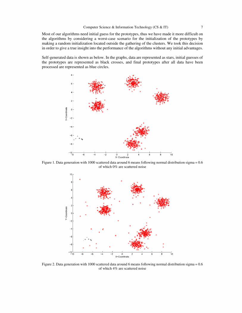
Most of our algorithms need initial guess for the prototypes, thus we have made it more difficult on
the algorithms by considering a worst-case scenario for the initialization of the prototypes by
making a random initialization located outside the gathering of the clusters. We took this decision
in order to give a true insight into the performance of the algorithms without any initial advantages.
Self-generated data is shown as below. In the graphs, data are represented as stars, initial guesses of
the prototypes are represented as black crosses, and final prototypes after all data have been
processed are represented as blue circles.
Figure 1. Data generation with 1000 scattered data around 6 means following normal distribution sigma = 0.6
of which 0% are scattered noise
Figure 2. Data generation with 1000 scattered data around 6 means following normal distribution sigma = 0.6
of which 4% are scattered noise

8 Computer Science & Information Technology (CS & IT)
In order to make performances of the algorithms comparable, we use the same sets of data for the
whole study. Examples are sequentially fed to generate the time-series data. In order to mimic the
sequential behavior of data, at each iteration, we will select a random point from the generated data
and do the processing on it.
First, we will test the proposed algorithms on the generated data without the presence of the noise
factor. Then we will introduce a uniform noise on our data and check the effect on each algorithm.
3.1. Study Without Noise
3.1.1. Implementation of Sequential K-means Algorithm
We implement the unforgetful one first. Select the initial prototypes randomly, and according to the
algorithm, they should spread to approach the ideal prototypes and form the 6 clusters.
Figure 3. Classification using Online K−means unforgetful with initializing means Randomly
We see from the results that only 3 prototypes have been updated and relocated from their initial
positions while the rest did not get updated. This is because that in the online K-means, the new
coming point gets allocated to the clusters defined by the closest prototype to the point (code
colored), and only this prototype gets updated. The major problem occurs when we initialize some
prototypes in such way they will never be the closest to the data points, hence they will never be
updated.
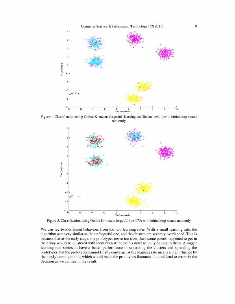
Then we run the forgetful one with different learning rates a = 0.1 and a = 0.75 separately.
Computer Science & Information Technology (CS & IT) 9
Figure 4. Classification using Online K−means forgetful (learning coefficient α=0.1) with initializing means
randomly
Figure 5. Classification using Online K−means forgetful (α=0.75) with initializing means randomly
We can see two different behaviors from the two learning rates. With a small learning rate, the
algorithm acts very similar as the unforgetful one, and the clusters are severely overlapped. This is
because that at the early stage, the prototypes move too slow thus, some points happened to get in
their way would be clustered with them even if the points don't actually belong to them. A bigger
learning rate seems to have a better performance in separating the clusters and spreading the
prototypes, but the prototypes cannot finally converge. A big learning rate means a big influence by
the newly-coming points, which would make the prototypes fluctuate a lot and lead to errors in the
decision as we can see in the result.

10 Computer Science & Information Technology (CS & IT)
Having noticed the difference in performances on the opening stage and the closing stages, we try
to put the two methods together. The process can be separated into 2 periods, while in the first
period a big learning rate is used to spread the prototypes as quickly as possible, and in the second
period, a small learning rate is taken to converge the prototype. At first, prototypes would spread
very quickly to avoid overlapping, and finally, a steady state would be reached.
In the following attempt, we use 300 points as the separation. In the first 300 points, the data are
clustered under a learning rate of 0.75 and then change to 0.1.
Figure 6. Classification using Online K−means forgetful (α�=0.75;α�=0.1) with initializing means randomly
Although the result is still not so convincing, but it's much better than the two forgetful ones at first
sight. Actually, the unforgetful K-means is based on the same idea of decreasing the learning rate
by steps, but this improved method stands out by its simplicity of calculation. We will use this
modified model for the calculating and the analyzing during the rest of this paper.
3.1.2. Implementation of the BSAS Algorithm
We try the BSAS with only one threshold and see its performance. To prevent the number of
clusters from exploding, we use an upper limit of 6 for cluster numbers. Set the threshold to 1, run
the code.

Computer Science & Information Technology (CS & IT) 11
Figure 6. Classification using BSAS with θ=1 and maximum of 6 clusters
The performance looks bad. It seems that there are too many clusters as the threshold is too small.
The threshold is increased to 3 and retest is done again.
Figure 7. Classification using BSAS withθ=3 and maximum of 6 clusters
The performance is much better, but this needs the knowledge of the right value for the threshold
apriori, which is not practical. In addition, in this test, we have not introduced the effect of the
noise. We will see later in the paper the catastrophic results when noise is introduced, new
misleading clusters will be created because of noise.
3.1.3. Implementation of the IWKO Algorithm
Let everything be the same except for the function to update the prototypes. In order to simplify the
calculation, set n in the function to be 2.

12 Computer Science & Information Technology (CS & IT)
Figure 8. Classification using Inverse Weighted K−means with initializing means randomly
The algorithm managed to spread the prototypes and find all the clusters which the k-means could
not. The drawback of this algorithm is that it needs several iterations at first as a learning phase
where it can spread the prototypes. During this learning phase, the algorithm will make mistakes in
allocating the coming data; this is evident by the mixed colors in one cluster. But once the
spreading phase is done the algorithm starts making the right decisions.
3.1.4. Implementation of the KHMO Algorithm
The KHMO method is very similar to the former ones with the same idea of spreading all the
prototypes in each step and with a simpler function.
Figure 9. Classification using Online K−Harmonics means (learning coefficient=0.05) with initializing
means randomly

Computer Science & Information Technology (CS & IT) 13
We can see it does succeed at finding the clusters the same way IWKO found them but with less
computation cost. The mixed points at the beginning also exists, showing another struggling
beginning to decide on the clusters.
3.2. Study with Noise
3.2.1. Implementation of K-means Algorithm
Do the same execution of K-means to the data set with noise. For the forgetful one, we use the
modified as it performs better without noise.
Figure 10. Classification using Online K−means unforgetful with initializing means Randomly
Figure 11. Classification using Online K−means forgetful (α�=0.75;α�=0.1) with initializing means randomly
14 Computer Science & Information Technology (CS & IT)
It seems noise doesn't affect the performance of K-means a lot. When the amount of data is huge, a
point of noise would have little effect on the mean. But no matter whether the noise exists, joint
clusters appears. This is caused by the isolation between examples, with only one prototype - the
one located nearest to the coming point - is changed. The truth is that if there are several clusters
squeezed somewhere and the initial prototypes are selected far away, when one prototype is moved
to this 'crowd', every point in the several clusters would be classified with this prototype as it is
always the 'nearest'. This is why we need the IWKO algorithm.
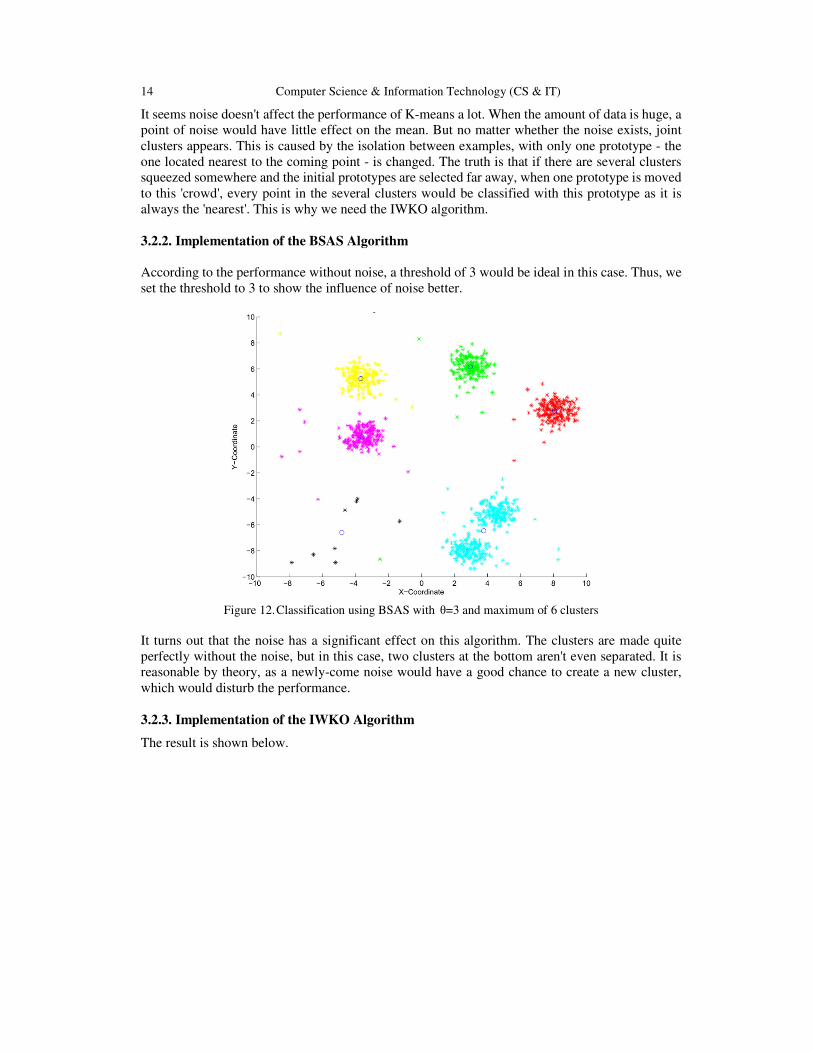
3.2.2. Implementation of the BSAS Algorithm
According to the performance without noise, a threshold of 3 would be ideal in this case. Thus, we
set the threshold to 3 to show the influence of noise better.
Figure 12. Classification using BSAS with θ=3 and maximum of 6 clusters
It turns out that the noise has a significant effect on this algorithm. The clusters are made quite
perfectly without the noise, but in this case, two clusters at the bottom aren't even separated. It is
reasonable by theory, as a newly-come noise would have a good chance to create a new cluster,
which would disturb the performance.
3.2.3. Implementation of the IWKO Algorithm
The result is shown below.

Computer Science & Information Technology (CS & IT) 15
Figure 13. Classification using Inverse Weighted K−means with initializing means randomly
Surprisingly, we find that the IWKO is vastly influenced by the noise. Every point has the influence
over all the prototypes, which means one single prototype has to 'tolerate' the harassment under all
the noise. This would be quite a lot if comparing to the ordinary K-means.
3.2.4. Implementation of the IWKO Algorithm
The result is shown below.
Figure 14. Classification using Online K−Harmonics means (learning coefficient=0.05) with initializing
means randomly
Though similar to the IWKO on the idea of the algorithm, they have quite different robustness. The
KHMO is not likely to be affected by noise, as the noise doesn't even change the result for
clustering. The difference mechanism between KHMO and IWKO might have saved KHMO. The
IWKO would find the nearest point and do the calculation, which means the calculation is different

16 Computer Science & Information Technology (CS & IT)
from time to time. This gives the noises chance to influence the result with there location and
sequences. While in the KHMO, every prototype changes under the same function. The noise
would have a similar influence to all the prototypes wherever it appears, and the result is relatively
honest.
4. ANALYSIS OF PERFORMANCES
The performance of algorithms is rated according to their execution speed, the accuracy of
prototypes, the purity of clusters and the robustness.
� The speed is indicated by the time MATLAB needs to get the result. We run each algorithm
several times, measure the time of each execution and take the average time of execution.
Here, we have run each program 20 times and took the average execution time. As the speed of
an algorithm is decided by the complexity of the algorithm itself rather than about the data
coming inside, there is no need to measure the time with noise included.
� The accuracy is the distance between the real prototypes and the clustered ones. The indicator
is calculated based on the average distance between each prototype after processing all the data
and the true means that were generated at the moment of data generation. This is a one-to-one
mapping between a prototype and its nearest true mean. The range of this indicator is a positive
value, and the bigger the better with 0 a perfect value.
� The purity is an indicator of the percentage of points that are rightly classified. It is shown by
the function[2]
P(ω, C) = 1Z� max� ]^� ∩ ��]�
where ω indicates the clusters (how actually the points are put together) and C indicates the
classes (howexactly the points should be put together). N is the total number of documents that
are correctly classified, and the value of sum should be the number of points that are correctly
classified. To get a better illustration, we generate different data set each time and calculate the
average purity as the purity of a certain algorithm. The indicator should be some value between
0 and 1, where 1 means perfectly clustered and 0 means the opposite. The noise is not
considered inside.
� The robustness is the ability to keep off the influence of noise. An indication of robustness is
based on the difference of velocity, accuracy, and purity between data sets with and without
noise. The formation of cluster shown above can also help. The bigger the difference, the
worse the robustness is. It can also be read from the graph in part 3.
Table 2. Performance of different algorithms.
Algorithms Noise Time Accuracy Purity Robustness
K-means
(forgetful)
0% 5.1119s 3.220 0.597 Good
4% 5.012 0.601
K-means
(unforgetful)
0% 5.1593s 6.160 0.495 Normal
4% 7.360 0.597
BSAS 0% 5.2966s 0.207 0.875 Bad
4% 1.540 0.739
IWKO 0% 5.6401s 0.648 0.766 Normal
4% 2.237 0.702
KHMO 0% 5.2472s 0.612 0.789 Good
4% 1.802 0.751
We can have some comment on the result.

Computer Science & Information Technology (CS & IT) 17
First, the velocity indicates how fast the system would respond to an input. It shows in the result
that the forgetful K-means has the most rapid response and the IWKO has the slowest. It is
consistent with what is shown by the theory. The IWKO and KHMO need to adjust position for
every prototype on each step, so it's reasonable the two of them takes relatively more time, and the
more steps of calculation made the IWKO even slower. The two K-means have to do nothing but
calculating and adjusting only one mean at a time, thus they are relatively fast; the forgetful wins as
it doesn't need to re-calculate the learning rate each time. At first, the BSAS seems confusing as its
algorithm is quite simple without too many calculations. It turns out that it uses more 'if' judgments
than the rest, which is quite costly.
Second, the accuracy shows how well-located the prototypes are. The results indicate that the
normal K-means are working really bad on locating the prototypes. The best performance comes
from the BSAS. This is because the BSAS has a good initial state by locating the point to
neighborhoods of the real prototypes. It would be better to relocate the prototypes inside a small
area rather than locate its step-by-step on the whole plane. The IWKO and the KHMO also stand
out by their idea of adjusting every prototype rather than only one; thus, it's nothing strange to find
them better than normal K-means.
Third, the purity is an indicator of how well the clusters are formed. The unforgetful K-means have
the purity of less than 0.5, which means less than half of the data are clustered correctly. This is a
disaster. The best performance comes from the BSAS because of the similar reason proposed in the
part of accuracy, but its performance drops significantly after noises invade. The forgetful K-means
seems almost not effect by the noise, but in general, the purity is too low. The IWKO and the
KHMO have relatively more stable behavior, while the KHMO has a higher level of purity.
Last, the robustness of BSAS is really bad. The most robust algorithm is the forgetful K-means,
with almost the same robustness. An interesting thing is that in the forgetful K-means algorithm,
the purity is even better than that without the noise. It is probable that in this case, noise help to
spread the initial prototypes, which would provide a better performance. We can also find out that
the forgetful K-means doesn't change a lot with the noise.
5. CONCLUSIONS
In this paper, we studied 4 different algorithms of sequential clustering. We explained the theory,
implemented them on self-generated data and analyzed their effectiveness. The implementation
could prove some of the characteristics shown by theory, and direct comparison between the
algorithms clearly reveals their pros and cons and preferred environment to be applied.
The sequential K-means stands out by its speed and robustness, as the mechanism and calculation
behind the algorithm is really simple; but its accuracy is a disaster as a result. The BSAS let the
system to start really near from the real prototypes, which would avoid a lot of error in the process
of 'finding' the prototypes, making itself an ideal choice for a clean dataset; but it would collapse
when noise is introduced. IWKO performs perfectly on getting accurate and robust results which is
guaranteed by its meticulous calculation, but its obvious slowness prevents it from becoming the
first choice. KHMO is quite moderate, doing well on very aspects with no prominent advantages or
shortcomings, making it a good algorithm in general.
To sum up, we can conclude thatwithout the noise, the Basic Sequential Algorithmic Scheme
(BSAS) would be the best algorithm among the four algorithms, but if noise is added, which is
always the case in real-life systems, the K-Harmonic Means- Online Mode Algorithm (KHMO)
would stand out with its robustness; if speed is the priority in a program, then the sequential
K-means should be adopted, but if one still considers accuracy so important that speed can be
sacrificed, IWKO would be a best choice.

18 Computer Science & Information Technology (CS & IT)
Our research can be improved in its depth and width. In depth, the four algorithms have not been
fully studied in this paper. The results are inevitably unstable as the generated data scale is too small
while the algorithms are always implemented on big data circumstances; implementation on bigger
datasets should make results more convincing. Two-dimension data are not common in real-life
applications, and performance of the algorithms in higher-dimension datasets might be more
accurate on results. In width, this paper only studied 4 algorithms but much more algorithms on
sequential clustering could also be studied under a same methodology. Performance evaluation is
still not strict, with several steps judged by sight, thus certain criteria should be constructed.
ACKNOWLEDGMENTS
The authors would like to thank our instructors and our universities.
REFERENCES
[1] S.Aghabozorgi ,A.Seyed Shirkhorshidi,and T.Ying Wah,(2015)“Time-series clustering - a decade
review”. Information Systems, vol.53, pp16-38.
[2] W.AshourBarbakh, Y.Wu, C.Fyfe, (2009)“Non-standard clustering criteria”. In Non-Standard
Parameter Adaptation for Exploratory Data Analysis, chapter 4, pages 49-72. Springer.
[3] T.Habib Sardar, Z.Ansari, (2018) “An analysis of MapReduce efficiency in document clustering using
parallel K-means algorithm”.Future Computing and Informatics Journal. pp1-10.
[4] X.Huang, Y.Ye, L.Xiong, R.Y.K.Lau, N.Jiang, S.Wang,(2018) “Time series K-means: A new k-means
type smooth subspace clustering for time series data”. Information Sciences, vol.367-368, pp1-13.
[5] C.Yang, N.T.P.Quyen,(2018) “Data analysis framework of sequential clustering and classification
using non-dominated sorting genetic algorithm”. Vol.69, pp 704-718.
[6] X.Zhao, F.Cao, J.Liang, (2018) “A sequential ensemble clusterings generation algorithm for mixed
data”. Vol.335, pp 264-277.
[7] H. Manning, Prabhakar Raghavan. Evaluation of clustering. An Introduction to Information Retrieval.
Cambridge University Press, 2008.
[8] Marcin Grzegorzek. Pattern Recognition Lecture: Sequential Clustering. Research Group for Pattern
Recognition, Institute for Vision and Graphics, University of Siegen, Germany.
[9] Department of Computer Science Princeton University. Sequential k-means clustering.
url: https://www.cs.princeton.edu/courses/archive/fall08/cos436/Duda/C/sk means.htm.
AUTHORS
Xinchun Yang, undergraduate student from Department of Electrical Engineering,
Tsinghua University, Beijing, China. Double major in economics in Peking University,
Beijing, China. Exchanging at CentraleSupélec, Paris, France in 2018..

Computer Science & Information Technology (CS & IT) 19
Wassim Kabbara, undergraduate student from Department of Energy Conversion,
CentraleSupélec University, Paris, France. Double diploma with Lebanese University
Faculty of Engineering, Electrical and Electronics Engineering.

20 Computer Science & Information Technology (CS & IT)
INTENTIONAL BLANK
Natarajan Meghanathan et al. (Eds) : DaKM, SIPP, CCSIT, NCWMC - 2018
pp. 21–36, 2018. © CS & IT-CSCP 2018 DOI : 10.5121/csit.2018.81502
IMPUTING ITEM AUXILIARY
INFORMATION IN NMF-BASED
COLLABORATIVE FILTERING
Fatemah Alghamedy1, Jun Zhang
2 and Maryam Al-Ghamdi
3
1,2Department of Computer Science,
University of Kentucky, Lexington, Kentucky, USA 3Department of Computer Science, University of Jeddah, Jeddah, Saudi Arabia
ABSTRACT
The cold-start items, especially the New-Items which did not receive any ratings, have negative
impacts on NMF (Nonnegative Matrix Factorization)-based approaches, particularly the ones
that utilize other information besides the rating matrix. We propose an NMF based approach in
collaborative filtering based recommendation systems to handle the New-Items issue. The
proposed approach utilizes the item auxiliary information to impute missing ratings before
NMF is applied. We study two factors with the imputation: (1) the total number of the imputed
ratings for each New-Item, and (2) the value and the average of the imputed ratings. To study
the influence of these factors, we divide items into three groups and calculate their
recommendation errors. Experiments on three different datasets are conducted to examine the
proposed approach. The results show that our approach can handle the New-Item's negative
impact and reduce the recommendation errors for the whole dataset.
KEYWORDS
Collaborative filtering, recommendation system, nonnegative matrix factorization, item
auxiliary information, imputation
.
1. INTRODUCTION
Nowadays, the world steps into new stages that depend mainly on technology. This appears in
many different fields, such as everyday life, work, and business. One of the most important
results of using technology in business is E-commerce. It has many helpful tools that are used to
figure out what the customer wants, such as recommendation systems (RS) [1] which suggest
items to users depending on the user’s preferences.
Recommendation systems (RS) are classified into three main categories: content-based (CB),
collaborative filtering (CF), and hybrid. The content-based (CB) system calculates the similarity
between items or users by utilizing external information, like user profiles and item descriptions.
The user gets recommendations for items that are similar to what he previously positively rated.
Since content-based RS does some manual intervention to collect the user profiles and items
descriptions, it is susceptible to errors and does not scale to large items basis. The collaborative
filtering (CF) finds users in the community who have same rated items in common. If two users
have the same rated items in common, it predicts that they will like the same items in the future.
CF doesn’t need any external information like the CB method. However, a number of approaches
combine these two systems, content-based (CB) and collaborative filtering (CF), into one system
to take the advantages of both of them and overcome their limitations.

22 Computer Science & Information Technology (CS & IT)
Collaborative filtering is the most popular approach because its results are more accurate than
other approaches and it needs fewer resources. Collaborative filtering algorithms are classified
into two main categories, memory-based methods and model-based methods.
Memory-based method, also called neighborhood-based method, relies on the rating of users or
items to compute the similarity. It has two types, user-oriented and item-oriented. User-oriented
CF computes the similarity between users based on their previous common items ratings, which
are known as user neighbors. If there are no common rated items between users, then user-
oriented CF will not be able to calculate the similarity, especially with cold-start users. Cold-start
users are users who did not rate a lot of items, e.g., less than five items. The system will not be
able to recommend items to them because it is hard to find neighbors for them. If we think about
the number of items that each user has rated, actually most users rate a small number of items
which makes the rating matrix suffer from sparsity and this leads to one of the most significant
issues which is called the rating matrix sparseness.
To overcome the memory-based method issues, model-based methods have been proposed.
Model-based algorithms model users based on their past items ratings. To predict missing ratings,
it employs statistical and machine learning techniques to learn models and use them. However,
memory-based RS doesn’t need to calculate the similarity and find the users’ neighbors. Model-
based algorithms also have the problem of data sparsity and still don’t solve the issue of cold-start
users.
Using only the rating matrix while letting aside all the other information sources in the dataset
will decrease the accuracy of the results. Examples of these information are: user information
(gender, occupation, location, interests, etc.), item categories, and social information (relationship
between users or trust and distrust list). Still, some other data analysis algorithms require
complete data.
Imputation is one of the approaches that has been used to complete missing data. The imputation
is the process of replacing missing data with substituted values [2]. The imputation method helps
recommendation systems to reduce rating matrix sparsity. Even though most recommendation
system methods do not require complete data, the imputation has been used. In the
recommendation system, if there are more ratings available in the rating matrix, the predicted
ratings are more accurate. Due to that fact, the imputation process has been used as a pre-
processing step in which missing data are imputed before the rating prediction process, then the
system predicts the rating based on original and imputed ratings. Prediction results using the
imputation data with an extremely sparse rating matrix often improves [3].
Even though the imputation alleviates the sparsity issue, it must be taken into consideration the
error, which may be introduced from the imputed ratings. To get the benefit of the imputation and
reduce the imputation error, we need to answer two important questions, (1) which missing data
should be imputed and (2) how to impute ratings [4]. For that, the most efficient imputation-based
collaborative filtering methods impute a subset of the missing data using strategies that select
which missing data should be imputed. There are several methods to impute missing data, such as
the ratings mean of either all known ratings or ratings of a particular item or user, and linear
regression. In addition, many imputation approaches have been proposed with both collaborative
filtering methods: memory-based and model-based collaborative filtering which are sometimes
called imputation-based collaborative filtering methods.
We propose a new strategy that handles New-Items issue by incorporating the item auxiliary
information with Aux-NMF without hurting other items prediction performance.

Computer Science & Information Technology (CS & IT) 23
The remainder of this paper is organized as follows. Section 2 shows the related work. Section 3
defines the problems and notations. Section 4 describes the main ideas of the proposed method.
Section 5 presents the datasets, experiments and discusses the results. Conclusions and future
work are given in Section 6.
2. RELATED WORKS
Nonnegative Matrix Factorization (NMF), which is based on the collaborative filtering method,
has been applied in the collaborative filtering. Zhang et al. in [5] used NMF to learn the missing
ratings in the rating matrix. A nonnegativity constraint is enforced in the linear model to
guarantee that all users’ ratings can be represented as an additive linear combination of canonical
coordinates. An unconstrained 3-factor NMF had been proposed by Ding et al. in [6] which has
an additional factor matrix to absorb the different scales in the two matrix factors in basic NMF.
It is insufficient to rely only on rating information because most datasets suffer from sparsity. In
addition, cold-start items which did not receive many ratings and cold-start users who did not rate
many items have the most negative impact. To alleviate this issue, other sources of information
have been used, such as user information [7] (gender, location, job title, interests, education level,
etc.), item categories [7], and social information (relationship between users or trust and distrust
list) [8, 9, 10, 11, 12]. Aux-NMF [7] is one of the studies that incorporates the users’ and items’
information into NMF method. Their proposed method surpasses the SVD-based data update
approach [13].
Moreover, the imputation process has been incorporated into collaborative filtering methods to
alleviate rating matrix sparsity. A method called IBCF had been proposed by Su et al. in [14] such
that a subset of missing data is imputed after dividing the rating matrix into subset matrices based
on the number of ratings each item received. A novel algorithm called (IMULT) had been
proposed in [15] based on the classic Multiplicative Update Rules (MULT), which utilizes
imputation to fill out the subset of unknown ratings. Furthermore, [16] proposed an imputation
method to impute New-Users. The results show that the proposed approach can handle the New-
Users issue and reduce the recommendation errors. Enlightened by these papers, we apply the
imputation process to Aux-NMF [7] by utilizing item auxiliary information. Our proposed
method is different from [16] in many aspects. First, we impute New-Items which focus on the
advertising beside the recommendation. In addition, we survey two factors that may affect the
imputation: (1) the total number of the imputed ratings for each New-Item, and (2) the value and
the average of the imputed ratings.
3. PROBLEM DESCRIPTION
In collaborative filtering, there are m users such that� = ���, … , ��and n items =���, … , ��.Each user� can rate a set of items. Users represent the rating through an explicit
numeric rating, such as a scale from one to five. In addition, the rating information is summarized
in an� × �matrix, which is called a rating matrix � ∈ ℝ�×�,1 ≤ � ≤ �, 1 ≤ � ≤ �. The rows in
the rating matrix represent the users, and the columns represent items. If a particular user� rates
a particular item��, then the value of the intersection of the user’s row and item’s column in the
rating matrix� � holds the rating value. If the rating is missing, that means the user did not rate
that item. Nonnegative Matrix Factorization (NMF) [17] is a dimension reduction method.
Nonnegative matrix tri-factorization (NMTF) is defined as follows [6],
��×� ≈ ��×� ∙ ��×� ∙ ��×�� (1)

24 Computer Science & Information Technology (CS & IT)
In NMTF, the rating matrix �is factoried into three matrices,�, � and �, where �is a matrix that
contains the latent factors for users and �contains the latent factors for items. In addition, �
matrix absorbs the different scales between � and �.Due to the fact that we are using Aux-NMF
as a basic algorithm, we need more matrices: the user feature matrix ! ∈ ℝ�×"# and the item
feature matrix % ∈ ℝ�×"& ,which hold the users’ and items’ information. Each user and item
belongs to one or more features '! and '%, respectively. The Aux-NMF is defined as follows [7],
���!(),*(),+(,-.�,/,�, �, �, 0! , 0%1 =
2 ⋅∥ / ∘ .� − ����1 ∥78+ : ⋅∥ � − 0! ∥78 + ; ⋅∥ � − 0% ∥78
(2)
where 2, : and; are coefficients that control the weight of each part. 0! and 0%are the user cluster
matrix and the item cluster matrix which are obtained by running the K-Means clustering
algorithm on the users feature matrix !and items feature matrix %. Generally, NMF cannot recommend items that did not receive any ratings to users. The values in
the row that represents this item in matrix �are zeros. Moreover, unpredictable ratings raise the
mean absolute error (MAE) especially when the average value of the ratings in the test set is
closer to the maximum rating value than the minimum. In our paper, we call the users that did not
rate any items New-Users and the items that did not receive any ratings New-Items.
Aux-NMF can alleviate this issue by adding the users and items cluster constraints such that in
each iteration of updating the matrices �, � and �, the : value is added to the � matrix and ; to �matrix. In this paper, we study the impact of the items auxiliary information constraint,;, in
Aux-NMF [7].
Our experiment shows that even though adding the items auxiliary information constraint can
alleviate the New-Items issue, other items’ MAE may become higher. We divide items into three
groups and calculate their MAE. The first group is New-Items which did not receive any ratings
at all. The second group is Cold-Start-Items which received at least one rating and at most four
ratings. The last group is Heavy-Rated-Items which received more than four ratings. We use the
training dataset to count the total number of ratings for each item - not the rating matrix -.In our
datasets, we observe that each group of items has different2 and ;values that result in the lowest
MAE. With New-Items group, all the datasets prefer to set ; to the maximum value, 0.9, and 2 to
the minimum, 0.1. This is because adding ; to the rows of New-Items in the � matrix allows the
system to recommend New-Items to users. The best MAE of Cold-Start-Items is when 2 = 1
and; = 0 with all datasets. However, the best Heavy-Rated-Items MAE results with different 2
and ; settings for each dataset. In addition, we observe that the percentage of the New-Items
ratings in the test set affects the best settings of 2 and ; for the whole dataset. If the percentage of
the New-Items in the test set is high, the Aux-NMF will rely more on items auxiliary information
constraint even if Cold-Start-Items and Heavy-Rated-Items MAE are getting worse.
We propose a method to impute a subset of New-Items ratings in the training set using the items
auxiliary information to alleviate the impact of New-Items on items auxiliary information
constraint and handle New-Items issue.
4. PROPOSED METHOD
We propose a new strategy that handles New-Items issue by incorporating the item auxiliary
information with Aux-NMF without hurting other items prediction performance. In addition, the
proposed method alleviates the impact of the New-Items on the items auxiliary information
constraint - γ-. Because imputed ratings introduce error to the system, our proposed method
imputes limited ratings for each New-Items whereas each dataset has a parameter of the
maximum imputed ratings for each New-Item.

Computer Science & Information Technology (CS & IT) 25
To perform the proposed method, we need to determine the subset of the real ratings that is used
to calculate the imputed ratings which are called source ratings, and the users who hold the
imputed ratings. For each user, we count the total ratings that the user did to all items that belong
to the same New-Item cluster based on the item cluster matrix %. After ordering the users based
on the total ratings descendingly, the top-N users are selected to hold the imputed ratings. For
each top-N user, only the user’s real ratings are utilized to calculate the imputed ratings. Thereby,
we ensure that we maintain the user rating pattern without involving other users’ ratings which
may have different rating pattern.
( a ) Rating matrix
( b ) Item cluster
matrix CI
( c ) Candidate
users
( d ) Total
ratings
( e) Imputed rating
matrix
Figure 1. A simple example of the imputation process.
Figure 1 is a simple example to illustrate the basic idea of the imputation. Figure 1 (a) is the
rating matrix that presents the users, items, and the users’ ratings to the items. As we see, item e3
is a New-Item because there is no rating for it. To impute e3, we need to find all items that belong
to the same cluster as e3. Figure 1 (b) displays the item cluster matrixCI. Item e3 belongs to
clusterG2 and items e1 and e2 belong to the same cluster as e3 belongs to. The candidate users that
may hold the imputed rating are u1 and u2 because they did rate at least one of e1 and e2 items
(Figure 1 (c)). User u1 rated two items while user u2 did one rating only that belong to cluster G2.
If we determine to impute one rating for each New-Item, then u2 will hold the imputed rating for
e3 because u2 did the highest number of ratings as we see in Figure 1 (d). The source ratings are
the ratings that are used to calculate the imputed rating. In our example, the ratings 5 and 1 of u2
are the source ratings. The average of the imputed source ratingsis 3. The imputed rating of user
u2 to New-Item e3 is equal to 3 as we see in Figure 1 (e).
In reality, introducing New-Items to the system is actually advertising items to the customers. For
that, the prediction error of the users that have a high probability to like the New-Item should be
less compared to the users that don’t. There are two methods to calculate the imputed ratings. The
first one is the average of the subset of the real ratings that are used to impute, source ratings, and
the second method is the most frequent rating appears in that subset.
1) Objective Function: Aux-NMF developed the objective function for weighted and constrained
nonnegative matrix tri-factorization that incorporates the auxiliary information of users and items,
as we see in Equation 2.
To handle the New-Item issue, we replace the rating matrix � with imputed rating matrix �′ such
that
? �@ = A? � , if? � ≠ 0ImputedRating, iftotalratingsofitem� = 0andsourceratings ≠ ∅0otherwiseX (3)
where ? �@ ∈ �@, ? � ∈ �, and Imputed Rating could be either the average of the source ratings or
the most frequent ratings.
In addition, we redefined /as a /@ such that:

26 Computer Science & Information Technology (CS & IT)
Y �@ = Z1, if? �@ ≠ 00, if? �@ = 0X [Y �@ ∈ /@, ? �@ ∈ �@\ (4)
By updating Equations (2) using Equations (3) and (4), the objective function is:
���!(),*(),+()-.�@,/@, �, �, �, 0! , 0%1 =
2 ⋅∥ /@ ∘ .�@ − ����1 ∥78+ : ⋅∥ � − 0! ∥78+ ; ⋅∥ � − 0% ∥78 (5)
We name this matrix factorization AuxNew-Item-NMF.
2) Update Formula: The derivation of update formula is the same as Aux-NMF [7] except we
replace the rating matrix �with the imputed rating matrix �′ and /with /′. The final update
formula is in Algorithm 1, Lines 12-14.
We suppose ], ^ ≪ ���.�, �1, the time complexities of updating �, �, and �in each iteration are
all`[��.] + ^1\. Thus, the time complexity of AuxNew-Item-NMF in each iteration
is`[��.] + ^1\. 3) Detailed Algorithm: In this section, we present the AuxNew-Item-NMF algorithm.Algorithm 1
depicts the steps of performing AuxNew-Item-NMF on the imputed rating matrix �′. We perform
this algorithm with two cases. The first case is when the imputed ratings are equal to the average
of source ratings which is called the Average-Imputation case. The second case is when the
imputed ratings are equal to the most frequent ratings in source ratings which is called Most-
Imputation case. However, it may take hundreds or thousands of iterations to converge to a local
minimum. Thus, in the algorithm, we set an additional stop criterion - the maximum iteration
counts. In collaborative filtering, this value varies from 10 ∼100 which can produce good results.
Algorithm 1 New-Item Imputation
Require:
User-Item rating matrix:� ∈ ℝ�×�; User feature matrix: ! ∈ ℝ�×�#; Item feature matrix: % ∈ ℝ�×�&; Column dimension of�:]; Column dimension of�:^; Coefficients in objective function:2, :and;; Number of maximum iterations: MaxIter; Number of maximum imputed ratings for each New-Item: MaxImputedRatings;
Ensure: Factor matrices: � ∈ ℝ�×�, � ∈ ℝ�×� , and� ∈ ℝ�×�; User cluster membership indicator matrix:0! ∈ ℝ�×�; Item cluster membership indicator matrix:0% ∈ ℝ�×� Imputed rating matrix:�@ ∈ ℝ�×�;
1: Function New-Items Imputation[�, 0%cde , �, f�g�hih�j�Case\ 2: for each group l%in0%cdedo
3: if l% == 1then
4: l%fh��m = l%fh��m+ all items belong to l% 5: end if
6: end for 7: for each user � do
8: candidateImputedUsers = count the total ratings of � for all items in l%fh��m 9: end for
10: OrderedUsers =sort candidateImputedUsers based on the total ratings indescending
order

Computer Science & Information Technology (CS & IT) 27
11: for� �nopqr = 1 ∶MaxImputedRatings in OrderUsers do
12: if Imputation Case =Average then 13: ?otuvwxyz�@ = the average ratings of � �nopqrfor all items inl%fh��m 14: else if Imputation Case = Most then 15: ?otuvwxyz�@ = the most frequent ratings value of � �nopqrfor all items inl%fh��m 16: end if 17: end for 18: return?:�@ 19: end function
1: Cluster users into k groups based on !by K-Means algorithm → 0!;
2: Cluster items into l groups based on %by K-Means algorithm → 0%; 3: InitializeU,S,andVwithrandomvalues;
4: for each item��do
5: if �� total ratings == 0then
6: ?:�@ =New-ItemsImputation(�, 0%y{: , �, ImputationCase)
7: end if
8: end for
9: Buildweightmatrix/@byEq.(4);
10: Set �h�?ih�j� = 1andmhjg = -i^m�;
11: while (�h�?ih�j� < }i~fh�?) and (mhjg == -i^m�) do
12: � � ⟵� � ⋅ ��[��∘��\+*����#�t{�����∘.!*+�1�+*���!t{
13: � � ⟵ � � ⋅ ��[��∘��\�!*���&�t{�����∘.!*+�1��!*��+t{ 14: � � ⟵ � � ⋅ �!�[��∘��\+�t{�!����∘.!*+�1�+t{ 15: � ⟵ 2 ⋅∥ /@ ∘ .�@ − ����1 ∥78+ : ⋅∥ � − 0! ∥78+ ; ⋅∥ � − 0% ∥78
16: if L increases in this iteration then
17: stop = true; 18: Restore U, S, and V to their values in last iteration. 19: end if 20: endwhile
21: Return R′,U,S,V,CU, and CI.
5. EXPERIMENTAL STUDY
In this section, we discuss the datasets’ description, evaluation strategy, and experimental results.
5.1. Data Description
Table 1. Statistics of the datasets.
Dataset # Users # Items # Ratings New-Items ratings % in the test set
CiaoDVD 17,615 16,121 72,345 13.22%
Ciao 7,375 21,978 184,024 0.57%
Epinions 22,166 15,000 180,889 5.34%

28 Computer Science & Information Technology (CS & IT)
In the experiments, we adopt CiaoDVD [18], Ciao [19], and Epinions [19] as the test data. Table
1 shows the statistics information of the datasets.
The CiaoDVD was crawled from ciao.co.uk, the DVD category, in December 2013 [18].
Thereare 17,615 users, 16,121 items and 72,345 ratings. Each DVD item belongs to one of the 17
genres. However, there is no information about users. Users are allowed to rate the items using 5-
scale integer ratings (from 1 to 5).
The Ciao dataset was crawled from Ciao.co.uk in May 2011 by Tang et al. in [19]. There are
7,375 users and 106,797 items. Each item belongs to one or more of 28 different categories.
However, there is no information about users. Due to the MATLAB memory limitation, we only
chose users who rated at least one item and items that received at least three ratings ending up
with 7,375 users, 21,978 items, and 184,024 ratings. The 5-scale integer ratings are used to rate
the items.
The Epinions dataset was collected by Tang et al. in May 2011 [19]. There are 22,166 users and
296,277 items. Each item belongs to one or more of 27 categories. However, there is no
information about users in this dataset. Due to the MATLAB memory limitation, we chose 15,000
out of 296,277 items, which are the first 5,000 items, the middle 5,000 items, and the last 5,000
items. Ending up with 22,166 users, 15,000 items and 180,889 ratings. Users are allowed to rate
the items using 5-scale integer ratings.
5.2. Evaluation Strategy
We compare the performance between the proposed approach AuxNew-Item-NMF and Aux-
NMF [7] using the Mean Absolute Error (MAE). The MAE is defined as:
}� = 1|��mh��h| � |? � − g �|�t{∈�q�p*qp (6)
where ? �is the actual value whileg �is the predicted value.
We use 80% of the ratings as a training set and 20% as a test set. We perform the imputation
process after the data is split into training and test sets, and we impute missing ratings using the
training ratings only. We perform our experiment in a 5-fold cross-validation approach. The
machine we used is equipped with a 2.53Ghz quad-core +HT processor, 8GB RAM and is
installed with UNIX operating system. The code was written and run in MATLAB.
5.3. Results and Discussion
To study the impact of the New-Items imputation process on predicting ratings and parameter
settings of Aux-NMF[7], we divide items into three groups and calculate their MAE: New-Items,
Cold-Start-Items, and Heavy-Rated-Items.
Some parameters of the proposed algorithms need to be determined in advance. Table 2 gives the
parameter setup in AuxNew-Items-NMF (see Algorithm 1).
Table 2. Parameter Setup in AuxNew-Items-NMF.
Dataset ββββ k l MaxIter MaxImputedRatings
CiaoDVD 0 2 15 10 3
Ciao 0 10 20 10 15
Epinions 0 10 20 10 5

Computer Science & Information Technology (CS & IT) 29
As mentioned before, with the none imputation case -Aux-NMF method-, the percentage of the
New-Items ratings in the test set affects the best settings of α and γ for the whole dataset. If the
percentage of the New-Items ratings is high, the system relies on items auxiliary information
constraint, γ, more than the rating matrix, because adding γ value to the � matrix allows the
system to predict the New-Items ratings and then recommend them to the users. However, the
other items’ group, Cold-Start-Items and Heavy-Rated-Items, may have different best settings of
α and γ. In addition, the difference in the MAE between the best setting of α and γ for the whole
dataset and each item group can be large. In this analysis, we demonstrate that imputing New-
Items helps to reduce the difference of MAE between the best setting of α and γ for the whole
dataset and for each item group.
Table 3. MAE results of the whole dataset and item groups with all selected combinations of α and γ of
both methods: Aux-NMF and AuxNew-Item-NMF.
αααα ββββ
All-Items MAE New-Items MAE Cold-Start-Items
MAE
Heavy-Rated-Items
MAE
Aux-
NMF
AuxNew-
Item-
NMF
Aux-
NMF
AuxNew-
Item-
NMF
Aux-
NMF
AuxNew-
Item-
NMF
Aux-
NMF
AuxNew-
Item-
NMF
CiaoDVD
0.1 0.9 2.0532 1.9011 2.6477 1.5036 1.8222 1.8153 2.0106 2.0118
0.2 0.8 2.0698 1.8918 2.8351 1.4921 1.7997 1.7951 2.0056 2.0066
0.3 0.7 2.0750 1.8853 2.9164 1.4839 1.7832 1.7799 2.0026 2.0034
0.4 0.6 2.0762 1.8801 2.9588 1.4771 1.7695 1.7671 2.0006 2.0012
0.5 0.5 2.0760 1.8758 2.9834 1.4708 1.7576 1.7558 1.9993 1.9998
0.6 0.4 2.0750 1.8721 2.9985 1.4647 1.7467 1.7454 1.9985 1.9988
0.7 0.3 2.0738 1.8689 3.0073 1.4588 1.7364 1.7357 1.9982 1.9983
0.8 0.2 2.0726 1.8664 3.0123 1.4532 1.7271 1.7267 1.9986 1.9986
0.9 0.1 2.0720 1.8649 3.0148 1.4486 1.7189 1.7187 2.0000 2.0001
1 0 2.1810 1.8660 3.8322 1.4474 1.7142 1.7140 2.0030 2.0036
Ciao
0.1 0.9 0.8158 0.8036 3.0171 0.8332 0.9207 0.9212 0.7486 0.7487
0.2 0.8 0.8083 0.7954 3.1542 0.8339 0.8942 0.8945 0.7489 0.7489
0.3 0.7 0.8029 0.7897 3.1828 0.8340 0.8752 0.8754 0.7495 0.7495
0.4 0.6 0.7986 0.7855 3.1849 0.8343 0.8603 0.8604 0.7501 0.7501
0.5 0.5 0.7952 0.7820 3.1849 0.8346 0.8478 0.8479 0.7508 0.7509
0.6 0.4 0.7924 0.7792 3.1849 0.8351 0.8370 0.8370 0.7518 0.7518
0.7 0.3 0.7901 0.7769 3.1849 0.8357 0.8273 0.8273 0.7529 0.7529
0.8 0.2 0.7882 0.7750 3.1849 0.8367 0.8183 0.8182 0.7544 0.7544
0.9 0.1 0.7867 0.7735 3.1849 0.8095 0.8381 0.8095 0.7562 0.7562
1 0 0.7911 0.7723 4.1654 0.8401 0.8007 0.8006 0.7586 0.7586

30 Computer Science & Information Technology (CS & IT)
Epinions
0.1 0.9 1.3005 1.2205 2.6663 1.1633 1.8002 1.7721 1.1912 1.193
0.2 0.8 1.2991 1.2077 2.8476 1.1302 1.6772 1.6589 1.1857 1.1871
0.3 0.7 1.2957 1.1997 2.9053 1.1018 1.5988 1.5858 1.1829 1.1839
0.4 0.6 1.2927 1.1938 2.9291 1.0762 1.5426 1.5326 1.1812 1.1819
0.5 0.5 1.2900 1.1892 2.9379 1.0539 1.4986 1.4909 1.1801 1.1805
0.6 0.4 1.2876 1.1857 2.9400 1.0350 1.4628 1.4565 1.1793 1.1795
0.7 0.3 1.2857 1.1827 2.9404 1.0174 1.4323 1.4275 1.1789 1.1788
0.8 0.2 1.2841 1.1802 2.9405 0.9986 1.4056 1.4030 1.1786 1.1786
0.9 0.1 1.2831 1.1781 2.9405 0.9752 1.3831 1.3822 1.1788 1.1788
1 0 1.3349 1.1780 3.9059 0.9653 1.3679 1.3674 1.1799 1.1801
Before the New-Items imputation, the best setting of the New-Items group is when α is equal to
the minimum value, 0.1, and γ is equal the maximum value, 0.9 in all datasets as we see in Table
3. After imputing New-Items with the average of the source ratings, the New-Items prediction
improves remarkably for all selected α and γ combinations in all datasets as we see in Table 3. In
addition, the best setting of CiaoDVD and Epinions New-Items group is α = 1 and γ = 0.
However, Ciao dataset has the same α and γ best setting of New-Items group before and after the
imputation. The best setting of α and γ for other items groups, Cold-Start-Items and Heavy-
Rated-Items, did not change for all datasets and the MAE is almost the same.
We observe that the best α and γ setting of New-Items group is the same as the item group that
MaxImputedRatings value within its limits. For example, each New-Item in CiaoDVD and
Epinions datasets is imputed with 3 and 5 imputed ratings, respectively, and the best α and γ
setting of New-Items of both datasets are equal to Cold-Start-Items group best setting. However,
the best α and γ setting of New-Items in Ciao dataset is the same as Heavy-Rated-Items because
each New-Item is imputed with 15 imputing ratings which make them as a Heavy-Rated-Item.
This explains the reason that the best α and γ setting of Ciao New-Items dataset did not change
after the imputation.
As we see in Table 3, the imputation process improves the results and the best α and γ settings are
different in all the datasets. After the imputation, Ciao and Epinions datasets rely totally on the
rating matrix with α = 1 and γ = 0. In addition, CiaoDVD dataset relies almost on the rating
matrix with α = 0.9 and γ = 0.1. The difference between MAE of the item groups with the best α
and γ setting of the whole dataset and of each item group is moot compared to the none
imputation case. Before New-Items imputation, the difference in Epinions dataset between the
lowest MAE of New-Items and MAE of the same group with the best α and γ setting of the whole
dataset is the highest, which is 0.2742. However, after the imputation, Ciao dataset has the most
difference which is between the lowest MAE of the Heavy-Rated-Items group and the MAE of
them with the best α and γ setting of the whole dataset, which is 0.0099.
As a conclusion, using item auxiliary information for imputation, not the NMF process, is a better
strategy.
5.4. The Impact of Imputed Rating Value
In this section, we demonstrate how the value of the imputed ratings and the average of all the
imputed ratings impact the results. There are two cases to calculate the imputed rating value. The

Computer Science & Information Technology (CS & IT) 31
first one is when the imputed rating value is equal to the average of the source ratings. We call
this case, New-Items Average-Imputation case. In the second case, the imputed rating value is
equal to the most frequent rating value that appears in the source ratings instead of the average.
We call this case New-Items Most-Imputation case. The predicted rating is zero when the system
cannot predict the rating which is called unpredictable ratings. This happens because of the
impact of the New-Users. After applying NMF, some of the New-Item rows in matrix V are zeros
even though all New-Items are imputed. For each rating value of New-Items in the test set, we
consider its MAE as a high value when it is larger than the whole dataset MAE. On the other
hand, we consider the MAE as a low value when it is equal to or lower than the whole dataset
MAE.
Table 4. The average of the imputed ratings with both New-Items imputation cases: Average and Most.
Dataset Average Most
CiaoDVD 3.63 4.04
Ciao 4.10 4.46
Epinions 3.89 4.3
By applying Average-Imputation case to Ciao dataset, 96.12% of the rating value 4 of New-Items
in the test set get low MAE which is the highest percentage among all other rating values, as we
see in Table 6. This is because of the average of the imputed ratings which is 4.10 as shown in
Table 4. With the second imputation case, the average of the imputed ratings increases up to 4.46.
The low MAE percentage of rating value 5 for New-Items in the test set increases from 55.41% to
85.40%, which is the highest percentage among all other rating values as we see in Table 6. On
the other hand, the low MAE percentage of the rating value 4 declines to 80.77%. Because the
imputed rating average of both imputation cases is above 4, none of the rating value 1 and 2 MAE
of New-Items in the test set are low even though there are few 1 and 2 imputing ratings in the
second imputation case as we see in Table 5.
Table 5. The percentage and average for each imputed rating value range with both imputation cases:
Average and Most.
Rating value
range CiaoDVD Ciao Epinions
> <= % average % average % average
New-Item Average-Imputation Case
0 1 0.00% N/A 0.00% N/A 0.00% N/A
1 2 0.00% N/A 0.04% 1.52 0.02% 2
2 3 20.06% 2.74 1.82% 2.67 2.71% 2.89
3 4 52.55% 3.55 39.32% 3.72 48.74% 3.56
4 5 27.39% 4.42 58.82% 4.40 48.52% 4.29
New-Item Most-Imputation Case
0 1 0.53% 1 0.18% 1 0.19% 1
1 2 0.34% 2 0.32% 2 1.36% 2
2 3 24.50% 3 4.29% 3 10.69% 3
3 4 44.13% 4 44.17% 4 44.14% 4
4 5 30.51% 5 51.04% 5 43.63% 5
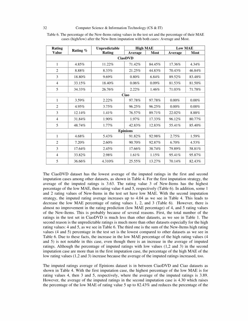
32 Computer Science & Information Technology (CS & IT)
Table 6. The percentage of the New-Items rating values in the test set and the percentage of their MAE
cases (high/low) after the New-Item imputation with both cases: Average and Most.
Rating
Value Rating %
Unpredictable
Rating
High MAE Low MAE
Average Most Average Most
CiaoDVD
1 4.85% 11.22% 71.42% 84.45% 17.36% 4.34%
2 8.88% 8.33% 21.25% 44.83% 70.43% 46.84%
3 18.80% 9.69% 0.80% 6.84% 89.52% 83.48%
4 33.15% 18.40% 0.06% 0.09% 81.53% 81.50%
5 34.33% 26.76% 2.22% 1.46% 71.03% 71.78%
Ciao
1 3.59% 2.22% 97.78% 97.78% 0.00% 0.00%
2 4.95% 3.75% 96.25% 96.25% 0.00% 0.00%
3 12.14% 1.41% 76.57% 89.71% 22.02% 8.88%
4 31.84% 1.90% 1.97% 17.33% 96.12% 80.77%
5 48.74% 1.77% 42.83% 12.83% 55.41% 85.40%
Epinions
1 4.68% 5.43% 91.82% 92.98% 2.75% 1.59%
2 7.20% 2.60% 90.70% 92.87% 6.70% 4.53%
3 17.64% 2.45% 17.66% 38.74% 79.89% 58.81%
4 33.82% 2.98% 1.61% 1.15% 95.41% 95.87%
5 36.66% 4.310% 25.55% 13.27% 70.14% 82.43%
The CiaoDVD dataset has the lowest average of the imputed ratings in the first and second
imputation cases among other datasets, as shown in Table 4. For the first imputation strategy, the
average of the imputed ratings is 3.63. The rating value 3 of New-Items has the highest
percentage of the low MAE, then rating value 4 and 5, respectively (Table 6). In addition, some 1
and 2 rating values of New-Items in the test set have low MAE. With the second imputation
strategy, the imputed rating average increases up to 4.04 as we see in Table 4. This leads to
decrease the low MAE percentage of rating values 1, 2, and 3 (Table 6). However, there is
almost no improvement in the rating prediction (low MAE percentage) of 4, and 5 rating values
of the New-Items. This is probably because of several reasons. First, the total number of the
ratings in the test set in CiaoDVD is much less than other datasets, as we see in Table 1. The
second reason is the unpredictable ratings is much more than other datasets especially for the high
rating values: 4 and 5, as we see in Table 6. The third one is the sum of the New-Items high rating
values (4 and 5) percentage in the test set is the lowest compared to other datasets as we see in
Table 6. Due to these facts, the increase in the low MAE percentage of the high rating values (4
and 5) is not notable in this case, even though there is an increase in the average of imputed
ratings. Although the percentage of imputed ratings with low values (1,2 and 3) in the second
imputation case are more than in the first imputation case, the percentage of the high MAE of the
low rating values (1,2 and 3) increase because the average of the imputed ratings increased, too.
The imputed ratings average of Epinions dataset is in between CiaoDVD and Ciao datasets as
shown in Table 4. With the first imputation case, the highest percentage of the low MAE is for
rating values 4, then 3 and 5, respectively, where the average of the imputed ratings is 3.89.
However, the average of the imputed ratings in the second imputation case is 4.30 which raises
the percentage of the low MAE of rating value 5 up to 82.43% and reduces the percentage of the

Computer Science & Information Technology (CS & IT) 33
low MAE of rating value 3 to 58.81%. As we observe in other datasets, there are more imputed
ratings of low values (1,2 and 3) in the second imputation case than the first one. However, the
low MAE percentage of the low rating values (1,2 and 3) decreases.
Table 7. The MAE of both New-Items imputation cases: Average and Most when α = 1.
Dataset Imputation
Case
All-Items
MAE
New-Items
MAE
Cold-Start-
Items MAE
Heavy-Rated-
Items MAE
CiaoDVD Average 1.8660 1.4474 1.7140 2.0036
Most 1.8700 1.4752 1.7152 2.0038
Ciao Average 0.7723 0.8400 0.8006 0.7586
Most 0.7720 0.7910 0.8006 0.7585
Epinions Average 1.1780 0.9653 1.3674 1.1800
Most 1.1796 0.9806 1.3711 1.1807
Table 7 shows the MAE results of both New-Items imputation cases: Average and Most when
α = 1 and γ = 0. We set MaxImputedRatings of both New-Items imputation cases as is shown in
Table 2. The results show MAE for the whole dataset and for each item group. Only MAE of
Ciao dataset is slightly lower with the New-Items Most-Imputation case than the Average-
Imputation case. This is because Caio dataset has the highest percentage of the rating value 5 in
the test set among other datasets (Table 6). In addition, the most improvement in the prediction in
the second imputation case is with rating value 5, as we see in Table 6. On the other hand, the
best MAE for other datasets is New-Items Average-Imputation case. For the New-Items group,
the results of Epinions and Ciao dataset are better with the second imputation case because the
strategy improves the prediction for the rating value 5 which reduces the error average. However,
the results of New-Items group in CiaoDVD dataset did not improve in the second imputation
case because there is no improvement in the prediction with any rating values as shown in Table
6.
As a conclusion, the prediction accuracy of the rating values that are close to the average of
imputed ratings is better than other rating values. In addition, the influence of the imputed rating
average is more effective than the value of the imputed ratings. Hence, the average of the imputed
ratings determines which rating values will have high or low MAE compared to the whole dataset
MAE. Because recommending New-Items to users considers as an advertisement, we think that
the users that have a high probability to like the New-Item need to have more accurate prediction
than the users that don’t. Raising the average of the imputed ratings allows the system to predict
the high rating values more accurately than the low rating values.
5.5. Parameter Study
(a) (b) (c) (d)
Figure 2. The MAE of New-Item Average-Imputation case with different values of
MaxImputedRatings when α = 1.

34 Computer Science & Information Technology (CS & IT)
In AuxNew-Item-NMF, the parameter MaxImputedRatings needs to be set. We run the
experiment with different total numbers of the imputed ratings for each New-Item. In this
experiment, we set α = 1 and γ = 0 with New-Item Average-Imputation case. In general, the MAE
of all three datasets are lower after New-Items imputation than all MAEs of all selected
combinations α and γ before the imputation regardless of the total number of imputed ratings,
MaxImputedRatings, as shown in Figure 2(a).
Mostly, adding more imputed ratings, MaxImputedRatings, improves the results of the New-
Itemsgroup prediction results slightly. Nevertheless, adding only one imputed rating to each New-
Item allows the system to recommend New-Items to users and reduces the New-Items MAE
remarkably compared to none imputation case as we see in Figure 2(b). When all available
imputed ratings are imputed for each New-Item, CiaoDVD and Ciao MAE are worse. However,
the result of Epinions dataset slightly improves but requires a long time to impute the rating
matrix. This demonstrates that adding imputed ratings is not always advantageous because they
introduce errors to the system at the same time even for New-Items.
As we see in Figure 2(d), the results of Heavy-Rated-Items show that more imputed ratings lead
to increase the MAE of them. However, there is a difference in the increment ratio of MAE
between the datasets. Ciao dataset has the lowest New-Items rating percentage in the test set
among other datasets, as we see in Table 1. For that, the Heavy-Rated-Items MAE did not
increase with the MaxImputedRatings increment but did increase when all possible imputed
ratings of New-Items are imputed. On the other hand, the highest percentage of New-Items
ratings in the test set among other datasets is in CiaoDVD dataset and Heavy-Rated-Items MAE
increases with each time the MaxImputedRatings is increased as shown in Figure 2(d). The New-
Items rating percentage in the test set of Epinions’s dataset is in the middle of Ciao and
CiaoDVD. As we see in Figure 2(d), there is an increment in the Heavy-Rated-Items MAE but
not with each time MaxImputedRatings is increased. Overall, the best of Heavy-Rated-Items
MAE is without imputation process.
In general, to set MaxImputedRatings parameter, we need to balance between the imputation
advantage and the imputation error that impacts Heavy-Rated-Items results. Table 2 shows the
best setting of MaxImputedRatings that improves the rating prediction of New-Items and limits
the error that may introduce to the other items. As we see from both Tables 1 and 2, there is an
inverse relationship between the best MaxImputedRatings parameter setting and the percentage of
New-Items ratings in the test set. CiaoDVD dataset has the most New-Items rating percentage in
the test set and the lowest MaxImputedRatings. On the other hand, Caio has the lowest New-Items
ratings percentage in the test set and the highest MaxImputedRatings.
6. CONCLUSION
In this paper, we proposed a method to incorporate item auxiliary information into the Aux-NMF
using the imputation process. Our results show that the proposed method allows the system to
recommend New-Items to the users. In addition, using item auxiliary information for imputation,
not the NMF process, is a better strategy. In addition, increasing the average of imputed ratings
improves the prediction accuracy of the users that have a high probability to like the New-Item.
As a future work, we want to study the behavior of other items group, i.e., Cold-Start-Items and
Heavy-Rated-Items with the imputation. In addition, we want to study the factors that affect the
best setting for each item group.

Computer Science & Information Technology (CS & IT) 35
REFERENCES
[1] P. Resnick and H. R. Varian, “Recommender systems,” Communications of the ACM, vol. 40, no. 3,
pp. 56–58, 1997.
[2] R. J. Little and D. B. Rubin, Statistical Analysis with Missing Data. Hoboken, New Jersey: John
Wiley & Sons, 2014.
[3] X.Su,T.M.Khoshgoftaar, and R.Greiner,“Imputed neighborhood based collaborative filtering,” in
Proceedings of the 2008 IEEE/WIC/ACM International Conference on Web Intelligence and
Intelligent Agent Technology-Volume 01, pp. 633–639, IEEE Computer Society, 2008.
[4] Y. Ren, G. Li, J. Zhang, and W. Zhou, “The efficient imputation method for neighborhood-based
collaborative filtering,” in Proceedings of the 21st ACM International Conference on Information and
Knowledge Management, pp. 684–693, ACM, 2012.
[5] S. Zhang, W. Wang, J. Ford, and F. Makedon, “Learning from incomplete ratings using non- negative
matrix factorization,” in Proceedings of the 2006 SIAM International Conference on Data Mining, pp.
549–553, SIAM, 2006.
[6] C. Ding, T. Li, W. Peng, and H. Park, “Orthogonal nonnegative matrix tri-factorizations for
clustering,” in Proceedings of the 12th ACM SIGKDD, pp. 126–135, ACM, 2006.
[7] X. Wang, J. Zhang, P. Lin, N. Thapa, Y. Wang, and J. Wang, “Incorporating auxiliary information in
collaborative filtering data update with privacy preservation,” International Journal of Advanced
Computer Science and Applications, vol. 5, no. 4, pp. 224–235, 2014.
[8] W.-S.Hwang,S.Li,S.-W.Kim,andK.Lee,“Dataimputationusingatrustnetworkfor recommendation,” in
Proceedings of the 23rd International Conference on World Wide Web, pp. 299–300, ACM, 2014.
[9] H. Ma, T. C. Zhou, M. R. Lyu, and I. King, “Improving recommender systems by incorporating social
contextual information,” ACM Transactions on Information Systems, vol. 29, no. 2, pp. 9:1– 9:23,
2011.
[10] J. He and W. W. Chu, “A social network-based recommender system (SNRS),” in Data Mining for
Social Network Data, pp. 47–74, Springer, 2010.
[11] H. Ma, I. King, and M. R. Lyu, “Learning to recommend with social trust ensemble,” in Proceedings
of the 32nd International ACM SIGIR Conference on Research and Development in Information
Retrieval, pp. 203–210, ACM, 2009.
[12] P. Massa and B. Bhattacharjee, “Using trust in recommender systems: an experimental analysis,” in
International Conference on Trust Management, pp. 221–235, Springer, 2004.
[13] X. Wang and J. Zhang, “SVD-based privacy preserving data updating in collaborative filtering,” in
Proceedings of the World Congress on Engineering, vol. 1, pp. 377–384, 2012.
[14] X. Su, T. M. Khoshgoftaar, X. Zhu, and R. Greiner, “Imputation-boosted collaborative filtering using
machine learning classifiers,” in Proceedings of the 2008 ACM Symposium on Applied Computing,
pp. 949–950, ACM, 2008.
[15] M. Ranjbar, P. Moradi, M. Azami, and M. Jalili, “An imputation-based matrix factorization method
for improving accuracy of collaborative filtering systems,” Engineering Applications of Artificial
Intelligence, vol. 46, pp. 58–66, 2015.
[16] F. Alghamedy, X. Wang, and J. Zhang, “Imputing trust network information in NMF-based
collaborative filtering,” in Proceedings of the ACMSE 2018 Conference, ACMSE ’18, (New York,
NY, USA), ACM, 2018.

36 Computer Science & Information Technology (CS & IT)
[17] D. D. Lee and H. S. Seung, “Algorithms for non-negative matrix factorization,” in Advances in
Neural Information Processing Systems, pp. 556–562, MIT Press, 2001.
[18] G. Guo, J. Zhang, D. Thalmann, and N. Yorke-Smith, “ETAF: An extended trust antecedents
framework for trust prediction,” in Advances in Social Networks Analysis and Mining (ASONAM),
2014 IEEE/ACM International Conference on, pp. 540–547, IEEE, 2014.
[19] J. Tang, H. Gao, and H. Liu, “mTrust: discerning multi-faceted trust in a connected world,” in
Proceedings of the Fifth ACM International Conference on Web Search and Data Mining, pp. 93–
102, ACM, 2012.
AUTHORS
Fatemah Algahmedy is Ph.D. candidate of computer science at University of Kentucky, USA and a
faculty at Imam Abdulrahman Bin Faisal University, Dammam, Saudi Arabia. She received her master
degree in computer science from Arkansas State University in USA. Her research interests machine
learning, data mining, recommendation systems, and biomedical informatics.
Dr. Jun Zhang received his Ph.D. from the George Washington University. He
is a professor in the Department of Computer Science at the University of
Kentucky. His research interests include, but are not limited to,data mining and
privacy, recommendation systems, large scale scientific computing and
applications.
Maryam Al-Ghamdi is a graduate student of computer science at University of Jeddah, Saudi Arabia.Her
research interests artificial intelligence, machine learning, human computer interaction, and web
development.

Natarajan Meghanathan et al. (Eds) : DaKM, SIPP, CCSIT, NCWMC - 2018
pp. 37–54, 2018. © CS & IT-CSCP 2018 DOI : 10.5121/csit.2018.81503
ENHANCE NMF-BASED
RECOMMENDATION SYSTEMS WITH
SOCIAL INFORMATION IMPUTATION
Fatemah Alghamedy and Jun Zhang
Department of Computer Science,
University of Kentucky, Lexington, Kentucky, USA
ABSTRACT
We propose an NMF (Nonnegative Matrix Factorization)-based approach in collaborative
filtering based recommendation systems to improve the Cold-Start-Users predictions since
Cold-Start-Users suffer from high error in the results. The proposed method utilizes the trust
network information to impute a subset of the missing ratings before NMF is applied. We
proposed three strategies to select the subset of missing ratings to impute in order to examine
the influence of the imputation with both item groups: Cold-Start-Items and Heavy-Rated-Items;
and survey if the trustees' ratings could improve the results more than the other users. We
analyze two factors that may affect results of the imputation: (1) the total number of imputed
ratings, and (2) the average of imputed rating values. Experiments on four different datasets
are conducted to examine the proposed approach. The results show that our approach
improves the predicted rating of the cold-start users and alleviates the impact of imputed
ratings.
KEYWORDS
Collaborative filtering, recommendation system, nonnegative matrix factorization, trust,
matrix, imputation
1. INTRODUCTION Recommendation systems [1] became an important tool in E-commerce because it can help both
sellers and buyers. The way it helps sellers is by increasing the profits and suggesting items to
customers. In addition, recommendation systems facilitate customers to find items they are
looking for easily.
Recommendation systems (RS) are classified into three categories: content-based (CB),
collaborative filtering (CF), and hybrid. The content-based (CB) system recommends items
similar to the user’s preference of the items in the past by utilizing external information, such as
item descriptions and user’s profiles to calculate the similarity between items or users. Since
content-based does some manual intervention to collect the user profiles and items descriptions, it
is susceptible to errors and does not scale to large items basis. On the other hand, collaborative
filtering (CF) supposes that users who agree on the items in the past agree in the future, too. CF
calculates the similarity measurement between users using their previous ratings of common
items. We can predict that two users will like the same items in the future if both have a high
similarity between their ratings in the past for the same items. One of the advantages of CF is
that there is no need for any external information like the CB method. The third category of RS

38 Computer Science & Information Technology (CS & IT)
combines content-based (CB) and collaborative filtering (CF) to merge the advantages of both
systems into one system and avoid each of the system’s limitations.
Collaborative filtering is the most popular approach because of the accuracy in prediction results
and fewer resources are required. Collaborative filtering algorithms are divided into two main
categories: memory-based methods and model-based methods.
Memory-based methods, also known as neighborhood-based methods, utilize the past and
common ratings between users for the same item (user-oriented CF) or common ratings between
items from the same user (item-oriented CF) to calculate the similarity measure. The issue with
this method arises if there are no common rated items between users thus similarity cannot be
calculated. The cold-start users who did not rate many items, e.g., less than five items often have
this issue and as a result, the system cannot recommend items.
To reduce the issues with the memory-based methods, model-based methods have been proposed
whereas users are modeled based on their past ratings by employing statistical and machine
learning techniques to learn models and use these learned models to predict the missing ratings.
In addition, model-based doesn't need to calculate the similarity and to find the users' neighbors.
However, the model-based algorithms still suffer from the data sparsity problem and fail to
address the cold-start users issue.
Relying only on the rating matrix and ignore other sources of information in the dataset that we
may use to increase the accuracy of the recommendation is irrational. There are several sources
that could be used such as user information (gender, job title, address, hobbies, etc.), item
categories, and social information (the relationship between users or trust and distrust list).
Traditional recommendation systems suppose that users are i.i.d. (independent and identically
distributed) and they ignore the connections among users which does not reflect the real world
recommendations.
Recommendation is considered as a social activity. For example, people usually ask a friend to
recommend movies to see or music to listen. Based on this research [2], friends in real life are
more qualified to advise good and useful recommendations than the traditional recommendation
system. In [3], Sinha and Swearingen showed that a user chooses recommendations from friends
over recommendation systems, in terms of quality and usefulness even if the recommendation
systems have a high novelty factor.
The relationship between the users’ taste and their friends’ taste has been observed by several
researchers such as Ziegler and Lausen demonstrated in [4] who concluded an empirical study of
a real online community. Their results showed that there is a similarity in the ratings between
users and their friends. Singla and Richardson in [5] analyzed over 10 million users on the social
network MSN Instant Messenger with their related search records and they concluded that there is
higher probable to have similar interests, such as the topics they are searching for, between the
users who chat with each other than the users who do not chat. In addition, the analysis of this
large dataset in [6] detected that friends have a tendency to give similar ratings to items.
In the beginning, users trust each other because they agree with their ratings and reviews. The
user that creates the trust relationship is called a trustor and the user that has been trusted is
named a trustee. After a while, the trustee influences the trustor even on some topics that they did
not agree on in the past [7]. In addition, [8] showed that most users participate in social networks
more than rating items.
Imputation is the process of replacing missing data with substituted values [9]. In addition, it is
one of the approaches that has been used to complete missing data, such as recommendation

Computer Science & Information Technology (CS & IT) 39
systems to reduce rating matrix sparsity. Most recommendation system methods do not require
complete data, but the imputation has been used because the predicted ratings are more accurate
when there are more ratings available in the rating matrix. In addition, the imputation process has
been used as a pre-processing step. Prediction results using the imputation data with an extremely
sparse rating matrix often improves [10].
It must be taken into a consideration the error that may be introduced from the imputed ratings. In
order to reduce the imputation error and benefit from the imputation, two factors must be taken
into the account, (1) which missing data should be imputed and (2) how to impute ratings [11].
The most efficient imputation-based collaborative filtering methods do not impute all missing
data by applying strategies to select which missing data should be imputed.
There are several imputation approaches that have been proposed with both collaborative filtering
methods: memory-based and model-based collaborative filtering. They are called imputation-
based collaborative filtering methods.
We propose a new approach to improve the cold-start users prediction results by reducing the
sparsity using the trust user network. In the review websites, users trust other users based on their
ratings since they don’t know that much of information about each other except the ratings. We
can expect that if a user did not provide a rating for an item, then his/her rating for that item will
be similar to his/her trustees’. We use the imputation process in the rating matrix by imputing a
missing rating with the average of the trust ratings for an item if there is at least one rating.
The remainder of this paper is organized as follows. Section 2 shows the related work. Section 3
defines the problems and notations. Section 4 describes the main ideas of the proposed method.
Section 5 presents the datasets, experiments and discusses the results. Conclusions and future
work are given in Section 6.
2. RELATED WORKS
Nonnegative Matrix Factorization (NMF) has been applied in the collaborative filtering. In [12],
Zhang et al. in used NMF to learn the missing values in the rating matrix which is based on the
collaborative filtering method. A nonnegativity constraint is enforced in the linear model to
guarantee that all users’ ratings can be represented as an additive linear combination of canonical
coordinates. Ding et al. proposed in [13] unconstrained 3-factor NMF which has an additional
factor matrix to absorb the different scales in the two matrix factors in basic NMF.
It is insufficient to rely on rating information only due to the fact that most datasets suffer from
sparsity. The most negative impact is shown with cold-start users who have not rated many items.
Other sources of information have been used in order to alleviate this issue, such as user
information (gender, occupation, location, interests, etc.), item categories, and social information
(relationship between users or trust and distrust list) [6, 14, 15, 16, 17]. Aux-NMF [18] is one of
the studies that incorporates the users’ and items’ information based on NMF method. Their
proposed method surpasses the SVD-based data update approach [19].
The social network is one of the sources that have been employed to alleviate the most serious
problems of the recommendation system: rating matrix sparsity and cold-start users. The social
network can be gathered from internal or external resources. There are review websites that allow
users to create a list of users whose reviews they suppose are trustworthy which is called a trust
list. Social relationship information has been incorporated into both memory-based [6, 17, 20]
and model-based collaborative filtering methods [16, 21].

40 Computer Science & Information Technology (CS & IT)
In [20], Massa et al. proposed a new method that incorporates social network into memory-based
collaborative filtering which substitutes the similarity measure with the trust metric to predict the
missing ratings. Rather than computing the similarity between two users based on their
commonly rated items, they computes the trust weight between users based on the trust web
network. The results show that their proposed method using only trust metrics is more effective,
in terms of accuracy and coverage than the purely collaborative filtering and the system that
combines trust and similarity, especially with cold-start users. In [16] they integrated the social
network structure and the user-item rating matrix based on probabilistic matrix factorization.
Moreover, the imputation process has been incorporated into collaborative filtering methods to
alleviate rating matrix sparsity. For example, IBCF is a method that has been proposed by Su et
al. proposed in [22] in which a subset of missing data is imputed after dividing the rating matrix
into subset matrices based on the number of ratings each item received. In addition, [23]
proposed a novel algorithm called (IMULT) based on the classic Multiplicative Update Rules
(MULT), which utilizes imputation to fill out the subset of unknown ratings.
In [21], they proposed a method to impute users in order to improve the ratings prediction.
However, the prediction improves only when New-Users are imputed, but not when All-Users are
imputed even though the prediction results of cold-start users with some datasets improved. This
indicates that imputing cold-start users could improve the prediction with some cases. In addition,
with New-Users imputation method, other users groups got worse results. In [14], they used the
trust network to impute missing ratings. The proposed method is based on the probabilistic matrix
factorization (PMF) model. Enlightened by these papers, we apply the imputation process to Aux-
NMF [18] by utilizing the trust network. Our proposed method is different from [14, 21] in the
missing data selection which we impute, and the known ratings which are used to impute the
missing ratings. In addition, we analyze two factors that may affect results of the imputation: (1)
the total number of imputed ratings, and (2) the average of imputed ratings value.
3. PROBLEM DESCRIPTION
In collaborative filtering, there are �users such that U = �u�, … , uand � items E = �e�, … , e�. Each user u� can rate a set of items. Users represent the rating through an explicit numeric rating,
such as a scale from one to five. In addition, the rating information is summarized in anm× n
matrix, which is called a rating matrix R ∈ ℝ×�, 1 ≤ i ≤ m,1 ≤ j ≤ n. The rows in the rating
matrix represent the users, and the columns represent items. If a particular user u� rates a
particular item e�, then the value of the intersection of the user’s row and item’s column in the
rating matrix R�� holds the rating value. If the user did not rate that item, then the rating will be
missing. Nonnegative Matrix Factorization (NMF) [24] is a dimension reduction method.
Nonnegative matrix tri-factorization (NMTF) is defined as follows [13],
��×� ≈ ��× ∙ " ×# ∙ $�×#% (1)
In NMTF, the rating matrix R is factoried into three matrices, U, V, and S, where U is a matrix that
contains the latent factors for users and Vcontains the latent factors for items. In addition, S
matrixabsorbs the different scales between Uand V. We divide users into three groups. The first
group isNew-Users who did not rate any items at all. The second group is Cold-Start-Users who
rated at leastone item and at most four items. The last group is Heavy-Rating-Users who rated
more than four items.
The social information is summarized in an m×m matrix, which is called the trust matrix T ∈ ℝ×, 1 ≤ p ≤ m, 1 ≤ q ≤ m. The rows correspond to the users who created a trust
relationship (trustor), and the columns correspond to the users who have been trusted by others
(trustee). If user u+ trusts user u,, the value of T+, is equal to 1. On the other hand, a zero in the

Computer Science & Information Technology (CS & IT) 41
trust matrix means there is no trust relationship between the users. Due to the fact that we are
using Aux-NMF [18] as a basic algorithm, we need more matrices: the user feature matrix F. ∈ ℝ×/0 and the item feature matrix F� ∈ ℝ�×/1, which hold the users’ and items’
information. Each user and item belongs to one or more features K. and K3, respectively. The
Aux-NMF is defined as follows [18],
�4�567,867,96:;<�,=,�, ", $, >5, >?@ =
A ⋅∥ = ∘ <� − �"$%@ ∥GH+ J ⋅∥ � − >5 ∥GH + K ⋅∥ $ − >? ∥GH
(2)
where A, Jand K are coefficients that control the weight of each part. >5 and >? are the user
cluster matrix and the item cluster matrix which are obtained by running the K-Means clustering
algorithm on the users feature matrix L5 and items feature matrix L?.
Generally, the Cold-Start-Users group suffers from a high error in the prediction results. In [21],
they proposed a method to impute users in order to improve the ratings prediction. When all
users are imputed with all available imputed ratings, some dataset’s prediction of Cold-Start-
Users improves with the imputation, however, the others do not. In this paper, we intend to study
the behavior of the non-New-Users groups with the imputation process and analyze the factors
that affect prediction when imputation process is used.
Our experiments show that the average of Cold-Start-Users ratings values in the training set is
higher than the whole dataset ratings average and Heavy-Rating-Users ratings average. In
addition, the average of the training set ratings of all users is higher than the mean of the rating
value. This indicates that users tend to rate items that they like more than items that they don’t.
This could be for several reasons. First, in the e-commerce era, it is easy for users to know all the
information that they need about the item before they make a decision to buy it. In addition, users
tend to trust their choices. Further, users tend to buy what they know such as a brand instead of
taking a risk and buying what they don’t know. In this case, users in reality did not try a lot of
options to make a fair rating. In general, Cold-Start-Users have higher MAE because of several
reasons. The first one is the lack of the ratings in the training set. The second reason is the
average of ratings value of the Cold-Start-Users in the training set because the Cold-Start-Users
ratings do not have a significant influence on the whole dataset rating average because of the lack
of Cold-Start-Users rating in the training set. In our proposed method, we have two goals: (1)
improve the Cold-Start-Users predictions (2) limit the impact of the imputed ratings. This could
be done by increasing the total number of the Cold-Start-Users rating and increasing the average
of the training set rating value through the imputed ratings, simultaneously.
4. PROPOSED METHOD
We propose a new method to improve the Cold-Start-Users predictions by incorporating the trust
information into Aux-NMF. In addition, the proposed method alleviates the impact of imputed
ratings in AuxTrsut-NMF, especially on Heavy-Rating-Users.
To perform the proposed method, we need to determine the subset of the real ratings that will be
used to calculate the imputed ratings which are called source ratings, and the items which will
hold the imputed ratings. The value of the imputed ratings equals the average of the ratings value
of the imputed user’s trustees for that item, i.e., the source ratings for each imputed rating is all
trustees’ ratings for the users that will be imputed.

42 Computer Science & Information Technology (CS & IT)
For each user group, we impute them with a limited number of imputed ratings to limit the error
that is introduced by the imputed rating. For each user, we consider the items that have been rated
by the user’s trustees as the candidate items that could be impute.
We have to select carefully which candidate items should be imputed because improving the
prediction results must be synchronized between the imputed user and the imputed item at the
same time. In addition, some items may be vulnerable to the error that is introduced by the
imputed rating more than others.
We have two factors that should be balanced between each other in order to select which item
should be imputed from candidate items: (1) the total number of the ratings from all users, and (2)
the total number of the ratings from only the user’s trustees.
The candidate items that received few ratings, which called Cold-Start-Items, share the same
issue with Cold-Start-Users, i.e., the lacking of the total number of ratings which results in less
accurate predicted ratings. For that, imputing Cold-Start-Items likely improves the prediction
results for the whole system as Cold-Start-Users.
On the other hand, the candidate items that received many ratings, called Heavy-Rated-Items,
could be considered as Heavy-Rating-Users who are affected by the imputed ratings negatively as
we see in [21].
To demonstrate our idea, we propose two strategies in which the candidate items are ordered
based on their total number of ratings ascendingly, which is called CSI case, and descendingly,
which is named HI case. For candidate items that have a tie total number of ratings, they are
ordered based on the total number of the ratings from the user’s trustees descendingly for two
reasons. First, allowing more source ratings in order to calculate the imputed ratings which means
more opinions from different trustees that results in more accurate imputed ratings. In addition,
candidate items that have been rated by many of the user’s trustees indicate that the user likely
agrees with trustees ratings more than candidate items that have been rated by few trustees
because many ratings from different trustee corroborate the opinion.
As we mentioned before, the pervious studies showed that there is a similarity in the ratings
between users and their friends [4]. In order to study the influence of the total number of the
ratings from the user’s trustees on the prediction results, we proposed another strategy in which
the candidate items are primarily ordered based on the total number of the ratings from the user’s
trustees descendingly then by the total number of the ratings for the item from all users
ascendingly which is called Trustee case. Table 1 show the summary of the three strategies.
Table 1. The summary of the three proposed cases.
Rating source All Users User’s trustee only
Order priority Order type Order priority Order type
Trustee 2 acs 1 desc
CSI 1 acs 2 desc
HI 1 desc 2 desc
1)Objective Function: In the proposed method, we replace rating matrix � in Equation 2 with the
imputed rating matrix �′ such that

Computer Science & Information Technology (CS & IT) 43
NOPQ = RNOP , ifNOP ≠ 0V�WXYZ[�\Y4�], 4;NOP = 0, V�WXYZ[�\Y4�] ≠ 0, \�[�ZZYYℎZ_`�[4Y4`�a0, `YℎZNb4aZ c (3)
wherer��Q ∈ RQ, r�� ∈ R, and Imputed Rating is the average of the source ratings if the rating r�� is
missing on rating matrix R and the imputed rating is not zero. In the proposed method, each users
group has a limited number of the imputed ratings and we have to make sure that the total number
of the imputed ratings for each user who does not exceed the parameter setting
In addition, we redefined Was a WQ such that:
bOPQ = f1, ifNOPQ ≠ 00, ifNOPQ = 0c gbOPQ ∈ =Q, NOPQ ∈ �Qh (4)
By updating Equation (2) using Equations (3) and (4), the objective function is:
�4�567,867,967;<�Q,=Q, �, ", $, >5 , >?@ = A ⋅∥ =Q ∘ <�Q − �"$%@ ∥GH+ J ⋅∥ � − >5 ∥GH+ K ⋅∥ $ − >? ∥GH (5)
We name this matrix factorization AuxTrustCSU-NMF, where CSU stands for Cold-Start-Users.
2) Update Formula: The derivation of update formula is the same as Aux-NMF [3] except we
replace the rating matrix � with the imputed rating matrix �′ and = with =′. The final update
formula is in Algorithm 1, Lines 47-49.
We suppose i, j ≪ �4�<�, �@, the time complexities of updating U, V, and S in each iteration are
all lg��<i + j@h. Thus, the time complexity of AuxTrustCSU-NMF in each iteration is lg��<i + j@h. 3) Detailed Algorithm: Algorithm 1 depicts the steps of performing AuxTrustCSU-NMF on the
imputed rating matrix R′. As we mentioned before, we perform the algorithm with three cases:
Trustee, CSI and HI. Because each user group in the proposed method has a limited total number
of the imputed ratings, we set three parameters which defined the total number of the imputed
ratings for each user group: m�V�, >"�V�,and n�V�. However, it may take hundreds or
thousands of iterations to converge to a local minimum. Thus, in the algorithm, we set an
additional stop criterion - the maximum iteration counts. In collaborative filtering, this value
varies from 10 ~ 100 which can produce good results.
Algorithm 1AuxTrustCSU-NMF
Require:
User-Item rating matrix: � ∈ ℝ�×�;
Trust matrix: o ∈ ℝ�×�; User feature matrix: L5 ∈ ℝ�× p;
Item feature matrix: L? ∈ ℝ�× q; Column dimension of � ∶ i;
Column dimension of $ ∶ j; Coefficients in objective function: A, JandK;
Total number of the imputed ratings for New-User group: m�V�;
Total number of the imputed ratings for Cold-Start-User group: >"�V�;
Total number of the imputed ratings for Heavy-Rating-User group: n�V�;
Number of maximum iterations: u\vVYZN;
Imputation Case: V�W>\aZ; Ensure:
Factor matrices: � ∈ ℝ�× , " ∈ ℝ ×#, and$ ∈ ℝ�×#;

44 Computer Science & Information Technology (CS & IT)
User cluster membership indicator matrix: >5 ∈ ℝ�× ; Item cluster membership indicator matrix:>? ∈ ℝ�×#; Imputed rating matrix: �Q ∈ ℝ�×�; 1: Cluster users into k groups based on L5 by K-Means algorithm → >5;
2: Cluster items into l groups based on L? by K-Means algorithm → >?; 3: InitializeU,S,andVwith random values;
4: for each userXOdo
5: find the user’s 4 trustees from the trust matrix o →yz 6: if _`X�Y<yz@ > 0then
7: find all items that have been rated by yz → _\�[4[\YZVYZ�a
8: if_`X�Y<_\�[4[\YZVYZ�a@ > 0then
9: for each _\�[4[\YZVYZ�a_Pdo
10: calculate the average of the rating values of yz users for item _P →V�WXYZ[�\Y4�]$\jXZ
11: count the total number of ratings for _P from all users → Y`Y\j�\Y4�]a|jj�aZNa
12: count the total number of ratings for _P from yz → Y`Y\j�\Y4�]aoNXaYZZa�aZNa
13: end for
14: if V�W>\aZ == oNXaYZZthen
15: Order _\�[4[\YZVYZ�a based on Y`Y\j�\Y4�]aoNXaYZZa�aZNadescendingly, then for the tie values
16: Order _\�[4[\YZVYZ�a based on Y`Y\j�\Y4�]a|jj�aZNaascendingly
17: else ifV�W>\aZ == >"Vthen
18: Order _\�[4[\YZVYZ�a based on Y`Y\j�\Y4�]a|jj�aZNa ascendingly, then
for the tie values
19: Order _\�[4[\YZVYZ�a based on Y`Y\j�\Y4�]aoNXaYZZa�aZNadescendingly
20: else ifV�W>\aZ == nVthen
21: Order _\�[4[\YZVYZ�a based on Y`Y\j�\Y4�]a|jj�aZNadescendingly, then
for the tie values
22: Order _\�[4[\YZVYZ�a based on Y`Y\j�\Y4�]aoNXaYZZa�aZNadescendingly
23: end if
24: if total ratings number of XO == 0 then
25: Y`WV�W�\Y4�]a = m�V�
26: else if total ratings number of XO > 0 AND total ratings number of XO < 5then
27: Y`WV�W�\Y4�]a = >"�V�
28: else if total ratings number of XO > 4 then
29: Y`WV�W�\Y4�]a = n�V�
30: end if
31: Set V�WXYZ[�\Y4�]>`X�YZN = 0
32: Set _\�[4[\YZVYZ�aV�[Zv = 0
33: whileV�WXYZ[�\Y4�]>`X�YZN < Y`WV�W�\Y4�]ado
34: � =index of _\�[4[\YZVYZ�a<_\�[4[\YZVYZ�aV�[Zv@ 35: if NO,P == 0then
36: NO,P == V�WXYZ[�\Y4�]$\jXZ<_\�[4[\YZVYZ�aV�[Zv@ 37: V�WXYZ[�\Y4�]>`X�YZN = V�WXYZ[�\Y4�]>`X�YZN + 1
38: end if
39: _\�[4[\YZVYZ�aV�[Zv = _\�[4[\YZVYZ�aV�[Zv + 1
40: end while
41: end if

Computer Science & Information Technology (CS & IT) 45
42: end if
43: end for
44: Build weight matrix =Q by Eq. (4);
45: Set 4YZN\Y4`� = 1andaY`W = ;\jaZ;
46: while(4YZN\Y4`� < u\vVYZN) and (aY`W == ;\jaZ) do
47: �OP ⟵ �OP ⋅ ��g��∘��h98����p��������∘<589�@�98���5�� 48: $OP ⟵$OP ⋅ ��g��∘��h�58���q��������∘<589�@��58��9�� 49: "OP ⟵ "OP ⋅ �5�g��∘��h9����5����∘<589�@�9�� 50: y ⟵ A ⋅∥ =Q ∘ <�Q − �"$%@ ∥GH+ J ⋅∥ � − >5 ∥GH+ K ⋅∥ $ − >? ∥GH
51: if L increases in this iteration then
52: aY`W == YNXZ 53: Restore �, " and $to their values in last iteration. 54: end if 55: endwhile 56: Return �Q, �, ", $, >5and>?.
5. EXPERIMENTAL STUDY
In this section, we discuss the datasets’ description, evaluation strategy, and experimental results.
5.1. Data Description
Table 2. Statistics of the datasets.
Dataset # Users # Items # Ratings # Trust Relationships
Ciao 7,375 21,978 184,024 111,781
CiaoDVD 17,615 16,121 72,345 22,484
Epinions 22,166 15,000 180,889 355,727
FilmTrust 1,642 2,071 35,494 1,853
In the experiments, we adopt four datasets. Ciao [25], CiaoDVD[26], Epinions [25], and
FilmTrust [27] as the test data. We adopt these datasets because they have the information that we
need to evaluate the proposed approach: the rating matrix� and trust matrixo.
Ciao is one of the popular review website that displays items from different online shopping
websites, such as Amazon and compares the prices from different shopping websites for the same
item. Users are allowed to rate items using 5-scaleinteger ratings (from 1 to 5) and trust each
other.When a user (trustor) agrees with another user’s reviews (trustee), then the trustor can insert
the trustee to his/her own trust list.
There are several datasets that have been extracted from the Ciao website. The first one is Ciao
dataset which was crawled from Ciao.co.uk in May 2011 by Tang et al. in [25]. There are 7,375
users and 106,797 items. Each item belongs to one or more of 28 different categories. However,
there is no information about users. Due to the MATLAB memory limitation, we only chose
users who rated at least one item and items that received at least three ratings ending up with
7,375 users, 21,978 items, and 184,024 ratings.

46 Computer Science & Information Technology (CS & IT)
The second one is Ciao DVD which was crawled from ciao.co.uk, the DVD category, in
December 2013 [26]. There are17,615 users, 16,121 items and 72,345 ratings. Each DVD item
belongs to one of the 17 genres. However, there is no information about users.
The Epinions dataset was collected by Tang et al. in May 2011 [25]. There are 22,166 users
and296,277 items. Each item belongs to one or more of 27 categories. However, there is no
information about users in this dataset. Due to the MATLAB memory limitation, we chose 15,000
out of 296,277items, which are the first 5,000 items, the middle 5,000 items, and the last 5,000
items. Ending up with 22,166 users, 15,000 items and 180,889 ratings. Users are allowed to rate
the items using 5-scaleinteger ratings.
FilmTrust was crawled from the entire FilmTrust website in June 2011 [27]. FilmTrust is a
website that provides predictive recommendations about movies. However, FilmTrust does not
recommend a list of movies to the users. Instead, FilmTrust suggests how much the user may like
a chosen movie [28].The FilmTrust dataset has 1,642 users, 2,071 items, 35,494 ratings, and
1,853 trust relationships. Therate is on a scale of a half star from half star to four stars.
5.2. Evaluation Strategy
We compare the performance between the proposed approach, Aux-NMF [18], and AuxTrust-
NMF [21] using the Mean Absolute Error (MAE). The MAE is defined as:
u|� = 1|oZaY"ZY| � |NOP − WOP|���∈%��z8�z (6)
whereNOPis the actual value whileWOPis the predicted value.
We use 80% of the ratings as a training set and 20% as a test set. We perform the imputation
process after the dataset is split into training and test sets, and we impute missing ratings using
the training ratings only. We perform our experiment in a 5-fold cross-validation approach. The
machine we used is equipped with a 2.53Ghz quad-core +HT processor, 8GB RAM and is
installed with the UNIX operating system. The code was written and run in MATLAB.
5.3. Results and Discussion
In this section, we present and discuss our experimental results. We compare our proposed
method with Aux-NMF [18] and with both cases of AuxTrust-NMF [21]: All-Users and New
Users imputation, too.
None of our datasets has information about users, so we set the users’ feature parameter, J,
tozero. However, using value impacts the weight of the rating matrix in the prediction process.
Toavoid that, we set the item features parameter, K, to zero to focus on the analysis of the
imputation effect.
Table 3. The MAE of Aux-NMF, New-Users Imp, and the proposed methods with the three cases.
Dataset Aux-NMF Aux-NMF All-
Users
Aux-NMF New-
Users Trustee CSI HI
Ciao 0.8237 0.8305 0.8224 0.8025 0.8029 0.8127
CiaoDVD 1.6503 1.6721 1.6462 1.6348 1.6368 1.6411
Epinions 1.0816 1.0751 1.0760 1.0382 1.0372 1.0448
FilmTrust 0.7288 0.7439 0.7269 0.7206 0.7200 0.7226

Computer Science & Information Technology (CS & IT) 47
Table 4. The percentage of each items group that are imputed in the training set with the three proposed
case: Trustee, CSI, and HI. CSI = Cold-Start-Items group; HI = Heavy-Rated-Items group
Proposed Case Trustee Case CSI Case HI Case
Item Group CSI HI CSI HI CSI HI
Ciao 49.96% 50.04% 84.63% 15.37% 4.16% 95.84%
CiaoDVD 42.26% 57.74% 95.75% 4.25% 4.18% 95.82%
Epinions 16.47% 83.53% 57.88% 42.12% 0.86% 97.38%
FilmTrust 32.90% 67.10% 51.16% 48.84% 2.15% 97.85%
In general, the results of the three cases of our proposed method are better than Aux-NMF and
AuxTrust-NMF: All-Users and New-Users with all datasets as we see in Table 3. Further, the
results of the CSI case are better than HI with all datasets. However, Ciao and CiaoDVD have
better results with Trustee case; and Epinions and FilmTrust are better with the CSI case. We
notice that the percentage of the Heavy-Rated-Items that are imputed in Epinions and FilmTrust
with Trustee case is very high compared to the other datasets as we see in Table 4. This indicates
that imputing Heavy-Rated-Items limits the advantages of the imputations.
On the other hand, when all users are imputed with all available imputed ratings in Aux-NMF
All-Users method, the results are the worst among all other methods expect Epinions dataset.
This is because Epinions has the highest difference between the New-Users before and after the
imputation which means the most imputed New-Users compared with the other datasets, as we
see in Table 9, which lead to the most improvement in the New-Users results.
Table 5. The MAE for whole dataset and each user group of Aux-NMF, AuxTrust-NMF: All Users and
New-Users, and the best case of the proposed method AuxTrustCSU-NM.
Methods All-
Users New-Users
Cold-
Start-
Users
Heavy-
Rating-
Users
Ciao
Aux-NMF 0.8237 4.4118 0.8345 0.7452
AuxTrust-NMF All-User 0.8305 1.4235 0.8399 0.7715
AuxTrust-NMF New-User 0.8224 1.3615 0.8345 0.7453
AuxTrustCSU-NMF Trustee 0.8025 1.3999 0.8118 0.7438
CiaoDVD
Aux-NMF 1.6503 4.3433 1.2397 1.0612
AuxTrust-NMF All-User 1.6721 4.2832 1.2722 1.1122
AuxTrust-NMF New-User 1.6462 4.2830 1.2442 1.0689
AuxTrustCSU-NMF Trustee 1.6348 4.2824 1.2302 1.0606
Epinions
Aux-NMF 1.0816 3.9203 1.0770 0.9316
AuxTrust-NMF All-User 1.0751 1.9541 1.0888 0.9769
AuxTrust-NMF New-User 1.0760 1.9495 1.0964 0.9543
AuxTrustCSU-NMF CSI 1.0372 1.9297 1.0529 0.9311
FilmTrust
Aux-NMF 0.7288 3.3677 0.7326 0.6455
AuxTrust-NMF All-User 0.7439 2.7780 0.7487 0.6679
AuxTrust-NMF New-User 0.7269 2.7735 0.7324 0.6463
AuxTrustCSU-NMF CSI 0.7200 2.7639 0.7242 0.6478

48 Computer
The New-Users group gets slightly better results than AuxTrust
worse in Ciao dataset as we see in Table 5. This could be because of the percentage of New
Users ratings in the test set that belong to New
the lowest among other datasets which allow imputing more missin
without concern about the error from the imputed ratings
When the Heavy-Rating-Users results in the proposed method are compared to Aux
5, we see that the results are slightly better with all datasets but not with
because the average of the ratings in the training set is the closest to the ratings mean among other
datasets as we see in Table 7. Increasing the average of the training ratings value after the
imputation leads to more error of the l
of the proposed method with AuxTrust
gets the highest improvement because the Heavy
New-Users imputation among other datasets. CiaoDVD dataset gets worse results with New
Users imputation but it improves with the proposed
FilmTrust, did not get much worse results with New
results with the proposed method is not notable. We conclude that the proposed
to handle the impact of the AuxTrust
Figure 1: Cold
The Cold-Start-Users results improve compared to the Aux
cases. We notice a proportional relationship between the percentage of the imputed Cold
Users in the training set and percentage of improvement in the results when the proposed method
is compared with the Aux-NMF method as we see in Table 5 and Figure 1. Ciao dataset has the
highest percentage of improvement in the results and the highest percentage of the imputed Cold
Start-Users in the training set. On the other hand, CiaoDVD has the lowe
improvement in the results and the
training set. However, when we compare the
datasets that have worse results with AuxTrust
imputed Cold-Start-Users in the training set get a better
even though Ciao has the highest percentage of the imputed
than Epinions, Epinions get a better percentage of improvement in
Epinions get worse MAE with New
with CiaoDVD and FilmTrust datasets.
MAE and capable to handle the impact of the AuxTrust
simultaneously.
Computer Science & Information Technology (CS & IT)
Users group gets slightly better results than AuxTrust-NMF New-Users method but it
worse in Ciao dataset as we see in Table 5. This could be because of the percentage of New
Users ratings in the test set that belong to New-Users that have been imputed in Ciao dataset is
the lowest among other datasets which allow imputing more missing ratings of New
from the imputed ratings.
Users results in the proposed method are compared to Aux
5, we see that the results are slightly better with all datasets but not with FilmTrust. This is
because the average of the ratings in the training set is the closest to the ratings mean among other
datasets as we see in Table 7. Increasing the average of the training ratings value after the
imputation leads to more error of the low ratings value. However, when we compare the results
of the proposed method with AuxTrust-NMFNew-Users imputation method, Epinions dataset
gets the highest improvement because the Heavy-Rating-Users group gets the worse results with
among other datasets. CiaoDVD dataset gets worse results with New
Users imputation but it improves with the proposed method, too. Other datasets, Ciao and
get much worse results with New-Users imputation thus the change in the
with the proposed method is not notable. We conclude that the proposed method
handle the impact of the AuxTrust-NMF imputation on the Heavy-Ratings-Users.
Figure 1: Cold-Start-User information in the training set.
improve compared to the Aux-NMF and AuxTrust-NMF
. We notice a proportional relationship between the percentage of the imputed Cold
Users in the training set and percentage of improvement in the results when the proposed method
NMF method as we see in Table 5 and Figure 1. Ciao dataset has the
highest percentage of improvement in the results and the highest percentage of the imputed Cold
Users in the training set. On the other hand, CiaoDVD has the lowest percentage of the
improvement in the results and the lowest percentage of the imputed Cold-Start-
training set. However, when we compare the proposed method to AuxTrust-NMF New
datasets that have worse results with AuxTrust-NMF New-Users and a high percentage of the
Users in the training set get a better result than other datasets. For example,
even though Ciao has the highest percentage of the imputed Cold-Start-Users in the training set
get a better percentage of improvement in the results than Ciao because
Epinions get worse MAE with New-Users AuxTrust-NMF method than Ciao. This is the same
with CiaoDVD and FilmTrust datasets. We conclude that imputing Cold-Start-Users reduces
handle the impact of the AuxTrust-NMF imputation on the Cold
Users method but it is
worse in Ciao dataset as we see in Table 5. This could be because of the percentage of New-
Users that have been imputed in Ciao dataset is
of New-Users
Users results in the proposed method are compared to Aux-NMF, Table
FilmTrust. This is
because the average of the ratings in the training set is the closest to the ratings mean among other
datasets as we see in Table 7. Increasing the average of the training ratings value after the
ow ratings value. However, when we compare the results
Users imputation method, Epinions dataset
Users group gets the worse results with
among other datasets. CiaoDVD dataset gets worse results with New-
. Other datasets, Ciao and
the change in the
method capable
NMF with both
. We notice a proportional relationship between the percentage of the imputed Cold-Start-
Users in the training set and percentage of improvement in the results when the proposed method
NMF method as we see in Table 5 and Figure 1. Ciao dataset has the
highest percentage of improvement in the results and the highest percentage of the imputed Cold-
st percentage of the
-Users in the
NMF New-Users, the
Users and a high percentage of the
result than other datasets. For example,
Users in the training set
the results than Ciao because
Ciao. This is the same
Users reduces
Cold-Start-Users

Computer Science & Information Technology (CS & IT) 49
Table 6. The average of the ratings value in the training set of the original rating matrix R for whole dataset
and each user group.
Dataset Whole Dataset Cold-Start-Users Heavy-Rating-Users
Ciao 4.1483 4.2164 4.1442
CiaoDVD 4.0711 4.2860 3.9369
Epinions 3.8742 3.9126 3.8640
FilmTrust 3.0028 3.1219 2.9954
Table 7. The average of the ratings value in the training set for whole dataset with Aux-NMF, AuxTrust-
NMF: All Users and New-Users, and the best case of proposed method AuxTrustCSU-NMF.
Dataset Aux-NMF AuxTrust-NMF
All-Users
AuxTrust-NMF
New-Users AuxTrustCSU-NMF
Ciao 4.1483 4.1870 4.1496 4.1569
CiaoDVD 4.0711 3.7887 4.0050 4.0720
Epinions 3.8742 3.8314 3.8382 3.9129
FilmTrust 3.0028 2.9376 2.9957 3.0032
As we see in Table 6, the average of Cold-Start-Users ratings value in the training set is higher
than the whole dataset ratings value average and Heavy-Rating-Users in all datasets. In addition,
the average of the training set ratings of all users is higher than the mean of the rating value.
With AuxTrust-NMF All-Users imputation case, the ratings average of the training set after the
imputation becomes lower in all dataset except Ciao. In addition, we notice that Cold-Start-Users
MAE in Ciao dataset has the lowest increase after the All-Users imputation among other datasets,
as we see in Tables 3 and 7.
With AuxTrust-NMF New-Users imputation case, the ratings value average of the training set is
higher than AuxTrust-NMF All-Users imputation case. However, Epinions dataset gets the
lowest increase in the rating average among other datasets, as we see in Table 7. The Cold-Start-
Users result is worse with AuxTrust-NMF New-Users imputation than AuxTrust-NMF All-Users
imputation case only in Epinions dataset compared to other datasets. This could be because of the
impact of the average of imputed ratings value.
The highest average of ratings values is with the proposed method AuxTrustCSU-NMF with all
datasets except Ciao, as we see in Table 7. In addition, the best prediction ratings are with
proposed. That indicates that the average of the ratings value in the training set has an important
influence on the accuracy of the rating prediction. There is a huge gap between the average of
original rating values and the highest average of rating values in Ciao which may result in
introducing error. That denotes the need to limit the increase in the average of rating values of
the training set.
5.3.1. Parameter Settings
As we mentioned before, we impute each user with a limited number of imputed ratings based on
the group that the user belongs to. In our experiment, we set the maximum imputed ratings for
each New-Users to 20, Cold-Start-Users to 5, and Heavy-Rating-Users to 3 imputed ratings.
Table 8 shows the total number of the imputed ratings for each users group that results in the
lowest MAE for the whole dataset.

50 Computer Science & Information Technology (CS & IT)
Table 8. The best parameters setting of the proposed method with the best case of each dataset.
Dataset Best Case New-Users Cold-Start Heavy-Users
Ciao Trustee 12 5 1
CiaoDVD Trustee 8 2 3
Epinions CSI 3 4 2
FilmTrust CSI 10 2 2
Table 9. The percentage of each users groupin the test set before and after the imputation.
User Group New-Users Cold-Start-Users Heavy-Ratings-Users
Imputation Case Before After Before After Before After
Ciao 0.05% 0.01% 86.43% 2.54% 13.52% 97.45%
CiaoDVD 13.92% 13.63% 73.95% 50.40% 12.12% 35.98%
Epinions 1.29% 0.43% 76.93% 23.77% 21.78% 75.80%
FilmTrust 0.30% 0.23% 86.19% 49.01% 13.50% 50.76%
For the New-Users group, there is an inverse relationship between the percentage of the New-
Users ratings in the test set that belong to New-Users that have been imputed and the best total of
imputed ratings of New-Users. Ciao dataset has the lowest percentage of the New-Users ratings
in the test set that belong to New-Users that have been imputed, 0.04%, and the highest total
number of imputed ratings among other datasets then FilmTrust comes after Ciao, as we see in
Tables 8 and 9. On the other hand, Epinions has the highest percentage of the New-Users ratings
in the test set that belong to New-Users that have been imputed, 0.89%, and the lowest total
number of imputed ratings among other datasets then CiaoDVD as we see in Tables 8 and 9. This
indicates that if we need to predict a lot of ratings for New-Users, we should take into the account
the percentage of the imputed New-Users to balance between the advantage of the imputed
ratings and the error that is introduced by the imputed ratings.
With the Cold-Start-Users group, there is a proportional relationship between the percentage of
imputed Cold-Start-Users in the training set and the total imputed ratings for each Cold-Start-
Users as we see in Figure 1 and Table 8. For example, there are more than 60% of Cold-Start-
Users in the training set of Ciao and Epinions datasets are imputed. In addition, the total number
of imputed ratings for each Cold-Start-Users of Ciao and Epinions datasets are higher than other
datasets: CiaoDVD and FilmTrust. The percentage of imputed Cold-Start-Users in the training
set are less than 30.5% with CiaoDVD and FilmTrust. This could be because the rating
prediction of the un-imputed Cold-Start-Users may hurt via imputed ratings. For that, we need to
reduce the imputed ratings for each Cold-Start-User if there is a high percentage of them could
not be imputed. In addition, the relationship between the percentage of imputed Cold-Start-Users
in the training set and the percentage of ratings in the test set that belong to imputed Cold-Start-
Users is proportional. Therefore, there is a proportional relationship between the percentage of
the Cold-Start-User ratings in the test set that belong to Cold-Start-Users that have been imputed
and the best total of imputed ratings of Cold-Start-User.
Even though Cold-Start-Users group results with the proposed method improve but not Heavy-
Rating-Users, both Cold-Start-Users and Heavy-Rating-Users groups are imputed. This could be
for several reasons. First, as we mentioned before, imputing Cold-Start-Items improves the
results more than imputing Heavy-Rated-Items. Because the candidate items are ordered based
on the total ratings from all users ascendingly, imputing Heavy-Rating-Users allows us to impute
more Cold-Start-Items. In addition, as we see in Table 10, the average of the ratings in the

Computer Science & Information Technology (CS & IT) 51
training set increases when we impute Heavy-Rating-Users which is one of the factors that results
in a lower MAE. However, it decreases in FilmTrust dataset when Heavy-Rating-Users are
imputed even though it results in a lower MAE. This is because the average of the ratings for
whole dataset and Cold-Start-Users in the training set are the closet to the ratings mean among
other datasets as we see in Table 6.
Table10. The average of ratings value in the training set with/without imputing Heavy-Rating-Users.
NUIR CSUIR HUIR Rating value
Ciao
12 5 1 4.1569
12 5 0 4.1548
CiaoDVD
8 2 3 4.072
8 2 0 4.0717
Epinions
3 4 2 3.9129
3 4 0 3.9035
FilmTrust
10 2 2 3.0032
10 2 0 3.0042
There is an inverse relationship between the percentage of imputed Cold-Start-Users in the
training set and the best setting of the imputed ratings of Heavy-Rating-User. In addition, there is
an inverse relationship between the best setting of the imputed ratings of Cold-Start-User and the
imputed ratings of Heavy-Rating-User. Ciao dataset has the highest percentage of imputed Cold-
Start-Users in the training set, highest imputed ratings for each Cold-Start-User, and the lowest
imputed ratings for each Heavy-Rating-User. On the other hand, CiaoDVD dataset has the lowest
percentage of imputedCold-Start-Users in the training set, lowest imputed ratings for each Cold-
Start-User, and the high estimputed ratings for each Heavy-Rating-User. FilmTrust and Epinions
datasets are in between. In general, the total of the best setting of the imputed ratings of Cold-
Start-User and Heavy-Rating-Users together in our experiment is in the same range which is
between four and six imputed ratings in total.
5.3.2. Results Summary
As a conclusion, handling the lack of the Cold-Start-Users and Cold-Start-Items ratings by
imputation could improve the rating prediction of them. It must be taken into consideration that
each imputed rating affects the average of the training ratings which subsequently affects the
prediction performance. In our experiment, the Cold-Start-Users ratings percentage in the test set
is really high which we believe that this kind of dataset represents the reality. On the other hand,
Cold-Start-Users ratings average in the training set does not have much influence on the whole
training set ratings average. This is due to the fact Cold-Start-Users suffer from a lack of the
ratings. We suggest using the proposed method with the systems that predict ratings of Cold-
Start-Users more than Heavy-Rating-Users.
6. CONCLUSIONS
In this paper, we proposed a method to incorporate social network information into the Aux-NMF
using the imputation process to improve the non-New-Users prediction results. We proposed
three strategies to select the subset of missing ratings to impute in order to examine the influence

52 Computer Science & Information Technology (CS & IT)
of the imputation with both item groups: Cold-Start-Items and Heavy-Rated-Items; and survey if
the trustees' ratings could improve the results more than the other users.
Our results show that imputing Cold-Start-Items improves the results of Cold-Start-Users with
AuxTrustCSU-NMF method, especially when the dataset suffers from Cold-Start-Users, but
worse at some others. However, two factors must be taken into account, the total number of the
imputed ratings and the average of the ratings in the training set after the imputation in order to
limit the imputed ratings error. However, our next step is to set the coefficients in AuxTrust CSU-
NMF and analyze the impact of user feature matrix and the item feature matrix on the imputed
rating matrix.
As a future work, we want to take the advantage of increasing the average of ratings values to
improve the prediction results without the need to set the maximum of the total imputed rating for
each user group.
REFERENCES
[1] P. Resnick and H. R. Varian, “Recommender systems,” Communications of the ACM, vol. 40, no. 3,
pp. 56–58, 1997.
[2] P. Bedi, H. Kaur, and S. Marwaha, “Trust based recommender system for semantic web.,” in
IJCAI’07 Proceedings of the 20th International Joint Conference on Artifical Intelligence, vol. 7, pp.
2677–2682, 2007.
[3] R. R. Sinha and K. Swearingen, “Comparing recommendations made by online systems and friends.,”
in DELOS Workshop: Personalisation and Recommender Systems in Digital Libraries, vol. 106,
2001.
[4] C.-N. Ziegler and G. Lausen, “Analyzing correlation between trust and user similarity in online
communities,” in International Conference on Trust Management, pp. 251–265, Springer, 2004.
[5] P. Singla and M. Richardson, “Yes, there is a correlation - from social networks to personal behavior
on the web,” in Proceedings of the 17th International Conference on World Wide Web, pp. 655–664,
ACM, 2008.
[6] J. He and W. W. Chu, “A social network-based recommender system (SNRS),” in Data Mining for
Social Network Data, pp. 47–74, Springer, 2010.
[7] D. Crandall, D. Cosley, D. Huttenlocher, J. Kleinberg, and S. Suri, “Feedback effects between
similarity and social influence in online communities,” in Proceedings of the 14th ACM SIGKDD
International Ionference on Knowledge Discovery and Data Mining, pp. 160–168, ACM, 2008.
[8] R. Forsati, M. Mahdavi, M. Shamsfard, and M. Sarwat, “Matrix factorization with explicit trust and
distrust side information for improved social recommendation,” ACM Transactions on Information
Systems, vol. 32, no. 4, p. 17, 2014.
[9] R. J. Little and D. B. Rubin, Statistical Analysis with Missing Data. Hoboken, New Jersey: John
Wiley & Sons, 2014.
[10] X.Su,T.M.Khoshgoftaar, and R.Greiner,“Imputed neighbourhood based collaborative filtering,” in
Proceedings of the 2008 IEEE/WIC/ACM International Conference on Web Intelligence and
Intelligent Agent Technology-Volume 01, pp. 633–639, IEEE Computer Society, 2008.
[11] Y. Ren, G. Li, J. Zhang, and W. Zhou, “The efficient imputation method for neighborhood-based
collaborative filtering,” in Proceedings of the 21st ACM International Conference on Information and
Knowledge Management, pp. 684–693, ACM, 2012.

Computer Science & Information Technology (CS & IT) 53
[12] S. Zhang, W. Wang, J. Ford, and F. Makedon, “Learning from incomplete ratings using non- negative
matrix factorization,” in Proceedings of the 2006 SIAM International Conference on Data Mining, pp.
549–553, SIAM, 2006.
[13] C. Ding, T. Li, W. Peng, and H. Park, “Orthogonal nonnegative matrix tri-factorizations for
clustering,” in Proceedings of the 12th ACM SIGKDD, pp. 126–135, ACM, 2006.
[14] W.-S.Hwang,S.Li,S.-W.Kim,andK.Lee,“Dataimputationusingatrustnetworkforrecommen- dation,” in
Proceedings of the 23rd International Conference on World Wide Web, pp. 299–300, ACM, 2014.
[15] H. Ma, I. King, and M. R. Lyu, “Learning to recommend with social trust ensemble,” in Pro- ceedings
of the 32nd International ACM SIGIR Conference on Research and Development in Information
Retrieval, pp. 203–210, ACM, 2009.
[16] H. Ma, T. C. Zhou, M. R. Lyu, and I. King, “Improving recommender systems by incorporating social
contextual information,” ACM Transactions on Information Systems, vol. 29, no. 2, 2011.
[17] P. Massa and B. Bhattacharjee, “Using trust in recommender systems: an experimental analysis,” in
International Conference on Trust Management, pp. 221–235, Springer, 2004.
[18] X. Wang, J. Zhang, P. Lin, N. Thapa, Y. Wang, and J. Wang, “Incorporating auxiliary informa- tion
in collaborative filtering data update with privacy preservation,” International Journal of Advanced
Computer Science and Applications, vol. 5, no. 4, pp. 224–235, 2014.
[19] X. Wang and J. Zhang, “SVD-based privacy preserving data updating in collaborative filtering,” in
Proceedings of the World Congress on Engineering, vol. 1, pp. 377–384, 2012.
[20] P. Massa and P. Avesani, “Trust-aware recommender systems,” in Proceedings of the 2007 ACM
Conference on Recommender Systems, pp. 17–24, ACM, 2007.
[21] F. Alghamedy, X. Wang, and J. Zhang, “Imputing trust network information in NMF-based
collaborative filtering,” in Proceedings of the ACMSE 2018 Conference, ACMSE ’18, (New York,
NY, USA), pp. 2:1–2:8, ACM, 2018.
[22] X. Su, T. M. Khoshgoftaar, X. Zhu, and R. Greiner, “Imputation-boosted collaborative filtering using
machine learning classifiers,” in Proceedings of the 2008 ACM Symposium on Applied Computing,
pp. 949–950, ACM, 2008.
[23] M. Ranjbar, P. Moradi, M. Azami, and M. Jalili, “An imputation-based matrix factorization method
for improving accuracy of collaborative filtering systems,” Engineering Applications of Artificial
Intelligence, vol. 46, pp. 58–66, 2015.
[24] D. D. Lee and H. S. Seung, “Algorithms for non-negative matrix factorization,” in Advances in
Neural Information Processing Systems, pp. 556–562, MIT Press, 2001.
[25] J. Tang, H. Gao, and H. Liu, “mTrust: discerning multi-faceted trust in a connected world,” in
Proceedings of the Fifth ACM International Conference on Web Search and Data Mining, pp. 93–
102, ACM, 2012.
[26] G. Guo, J. Zhang, D. Thalmann, and N. Yorke-Smith, “ETAF: An extended trust antecedents
framework for trust prediction,” in Advances in Social Networks Analysis and Mining (ASONAM),
2014 IEEE/ACM International Conference on, pp. 540–547, IEEE, 2014.
[27] G. Guo, J. Zhang, and N. Yorke-Smith, “A novel bayesian similarity measure for recommender
systems,” in IJCAI Proceedings of the Twenty-Third International Joint Conference on Artificial
Intelligence, pp. 2619–2625, 2013.

54 Computer Science & Information Technology (CS & IT)
[28] J.Golbeck,J.Hendler,etal.,“FilmTrust:Movierecommendationsusingtrustinweb-basedsocial networks,”
in Proceedings of the IEEE Consumer Communications and Networking Conference, vol. 96, pp.
282–286, 2006.
AUTHORS Fatemah Algahmedy is Ph.D. candidate of computer science at University of Kentucky, USA and a
faculty at Imam Abdulrahman Bin Faisal University, Dammam, Saudi Arabia. She received her master
degree in computer science from Arkansas State University in USA. Her research interests machine
learning, data mining, recommendation systems, and biomedical informatics.
Dr. Jun Zhang received his Ph.D. from the George Washington University. He is a
professor in the Department of Computer Science at the University of Kentucky. His
research interests include, but are not limited to, data mining and privacy,
recommendation systems, large scale scientific computing and applications

Natarajan Meghanathan et al. (Eds) : DaKM, SIPP, CCSIT, NCWMC - 2018
pp. 55–71, 2018. © CS & IT-CSCP 2018 DOI : 10.5121/csit.2018.81504
DISASTER INITIAL RESPONSES MINING
DAMAGES USING FEATURE EXTRACTION
AND BAYESIAN OPTIMIZED SUPPORT
VECTOR CLASSIFIERS
Yasuno Takato, Amakata Masazumi, Fujii Junichiro and Shimamoto Yuri
Research Institute for Infrastructure Paradigm Shift (RIIPS),
Yachiyo Engineering, Co. Ltd., Tokyo, Japan
ABSTRACT
Whenever a natural disaster occurs, it is important to quickly evaluate the damage status in
high-priority locations. Frequently, owing to the restrictions imposed by the availability of
disaster management resources, spatial information is predicted where the infrastructure
manager makes an initial response. It is critical that an initial response be effective to mitigate
social losses. In recent years, Japan has experienced several great earthquakes with magnitudes
of around 6, most notably the Great East Japan earthquake of March 2011 (M9), as well as
those striking Kumamoto (April 2016 (M7)), Osaka (June 2018 (M6.1), and Hokkaido
(September 2018 (M6.7)). These huge earthquakes occur not only in Japan but around the
world, with an earthquake and tsunami striking Indonesia as recently as October 2018. The
initial response to future earthquakes is an important issue related to knowledge of natural
disasters and to predict the degree of damage to infrastructure using multi-mode usable data
sources. In Japan, approximately 5 million CCTV cameras are installed. The Ministry of Land,
Infrastructure and Transportation uses 23,000 of these cameras to monitor the infrastructure in
each region. This paper proposes a feature extraction damage classification model using
disaster images with five classes of damage after the occurrence of a huge earthquake. We
present a support vector damage classifier for which the inputs are the extracted damage
features, such as tsunami, bridge collapses, and road damage leading to a risk of accidents,
initial smoke and fire, and non-disaster damage. The total number of images is 1,117, which we
collected from relevant websites that allow us to download records of huge earthquake damage
that has occurred worldwide. Using ten pre-trained architectures, we have extracted the
damage features and constructed a support vector classification model with a radial basis
function, for which the hyper parameters optimize the results to minimize the loss function value
with an accuracy of 97.50%, based on the DenseNet-201. This would provide us with further
opportunities for disaster data mining and localized detection.
KEYWORDS
Disaster Response, Damage Mining, Feature Extraction, Support Vector classifier, Bayesian
Optimization

56 Computer Science & Information Technology (CS & IT)
1. INTRODUCTION
This section reviews the related papers and works related to natural disaster management and
machine learning for disaster data resources. The authors highlight earthquake disasters and the
mining of five classes of earthquake damage data sets.
1.1. Literatures Related to Disaster Management
Manzhu et al. [1] reviewed the major big data sources and the associated achievements in disaster
management phases to monitor and detect natural hazards, and to mitigate disaster damage, as
well as the recovery and reconstruction processes. This paper focuses on the urgent response
phase after an earthquake in which damage is monitored and detected to make the decisions
needed to address initial rapid actions regarding high priority infrastructures such as roads,
intersections, bridges, river gates, and urban and rural areas. During 2014–2016, a variety of data
sources could be observed in articles, when the topic of big data was popular in disaster
management. These data sources are as follows: satellite, social media, crowd sourcing, sensor
web and IoT, mobile GPS, simulation, unmanned aerial vehicles (UAV), Light Detection and
Ranging (LiDAR), and spatial data. Among these digital data sources, satellite imagery [2][3] and
social media [4][5] data serve as the most popular data for disaster management.
However, a satellite used for remote sensing always moves slowly, such that there is a delay
between the times at which data is acquired. The resulting series of photographs is thus not useful
for recognizing earthquake features. Therefore, disaster detection can be done based on social
media: Twitter is used as a source of text mining, and spatial temporal analysis. However, social
media users cannot always monitor disaster damage accurately. Also, users tend to be agitated
and fearful for their safety after the occurrence of a huge earthquake. Messages sometimes lack
essential details owing to noise and may start false rumors. Therefore, this study focuses on
closed-circuit television (CCTV) data sources for monitoring damage to critical infrastructure in
order to make decisions related to high-priority responses.
1.2. Works Related to Disaster Images
CCTV cameras are being set up around real-world places such as houses for crime prevention,
industrial processes to detect anomalies, banks for security, shopping stores, schools, rail stations
for safety, traffic monitoring, sports events, and offices to monitor employees. CCTV, also known
as video surveillance, involves the use of video cameras to transmit a signal to a specific place
with a set of monitors. The first CCTV system was installed by Siemens AG at Test Stand VII in
Nazi Germany in 1942 for observing rockets [6]. The earliest video surveillance systems involved
constant monitoring because there was no means of recording and storing the information. A
modern machine vision system enables the constant monitoring of infrastructures and determine
whether earthquake disaster damage has occurred, with several cameras recording
simultaneously, with features such as time lapse and motion-activated recording. The resulting
savings in time and cost had resulted in an increase in the use of CCTV. Recently, CCTV
technology has been enhanced with a shift towards Internet-based products. There were an
estimated 350 million surveillance cameras worldwide as of 2016, compared with 160 million in
2012 [7]. Sixty-five percent of the CCTV cameras installed around the world are in Asia. There
are currently five million CCTV cameras installed in Japan. This enables the creation of systems

Computer Science & Information Technology (CS & IT) 57
to support decisions related to immediate initial responses with respect to high-priority locations
if a large earthquake were to occur.
As a low level approach, both the input and output are images, with several techniques for
analyzing changes that are detected after a disaster. Supannee et al. [8] presented a building
detection process that could detect damage to both small and large buildings with 75% accuracy.
That method was applied to obtain data from the 2004 tsunami that struck the coast of Thailand.
However, only one class of building was analyzed and the satellite images, which were limited to
the coastal area, had a 1-meter resolution. Ranga et al. [9] presented a probabilistic detection
system that provides information regarding changes in an area and which minimizes the post-
detection threshold procedure often required in traditional change-detection algorithms. However,
their method was intended for land use detection such as growth, loss, and no change. Maeda et
al. [10] proposed a method that uses CCTV images with reduced background noise and subtracts
the change between the ex ante and ex post when an earthquake occurs. A low-level application
contains simple algorithms that may be unstable and not highly accurate. This method has certain
disadvantages, making it important to optimize the thresholding parameter and the balancing
trade-off between the damaged signal and the background noise detection.
Figure 1. A thumbnail of QuakeV datasets randomly chosen 100 images

58 Computer Science & Information Technology (CS & IT)
On the other hand, as a high-level approach of a level equal to human vision, Kataoka et al.[11]
surveyed 1,600 studies of computer vision and devised the concept of semantic change detection
regardless of whether a building is damaged or not after an earthquake. However, that conceptual
method requires hundreds of thousands or even millions of disaster-image datasets; further, there
is no proof of the concept of semantic segmentation focusing on buildings and change detection
regarding damaged buildings. Also, we cannot obtain a middle-level application to classify
earthquake disaster images, owing to the lack of datasets addressing the instant at which an
earthquake occurs. The present study addressed middle-level image analysis where the input is
CCTV images in the order of thousands, and the output is disaster-class labels for decision
support with respect to the initial response to be applied to high-priority locations.
1.3. Mining of Earthquake Damage Datasets
With regard to disaster image datasets, NOAA [12] offers a natural-hazard image database with
1,163 photo images of 67 earthquake events that have occurred in the 100 years from 1915 to
2015. It enables the viewing of a gallery of images from each earthquake event. The database
includes earthquake disaster images from around the world, including the USA, Mexico,
Guatemala, Colombia, Nicaragua, Peru, Chile, Haiti, Ecuador, Russia, Iran, Turkey, Pakistan,
Algeria, Romania, Italy, Papua New Guinea, Australia, New Zealand, Samoa, China, Indonesia,
Taiwan, and Japan. However, the viewpoints differ, such as satellite images with low resolution,
airplane downward views, views of damage captured outdoors and indoors, as well as of
destroyed homes. In short, their focuses and viewpoints are wide ranging, while the privately
captured historical photos were taken without any unified rules. For each event, there are only a
limited number of images at the half 30 earthquake events on that database. Almost all of the
images were recorded after the earthquakes had occurred, while it took more than one week for
academic surveys to obtain the relevant data. We attempted to collect open-source web pages
from which earthquake damage images could be downloaded.
This paper highlights four earthquake disaster features such as tsunami damage, bridge collapses,
road damage giving rise to accident risks, and initial smoke and fire. The total number of
earthquake disaster feature datasets collected by the authors was 1,117. This paper focuses on
earthquake images, which we used to build a dataset named QuakeV. Figure 1 shows thumbnails
of the earthquake damage image dataset for which the validation data are randomly chosen with
100 images of each of the above classes.
2. DISASTER DAMAGE CLASSIFICATION
This section proposes a means of disaster damage classification using image data sets. The
disaster damage data are extracted into features using a pre-trained deep network. The features
output from a concatenated layer are used as an input to the support vector classification model
with more than two classes. To minimize the prediction error, the authors applied a Bayesian
optimization method for hyper parameters to enable a warm start based on the result of previous
training runs.

Computer Science & Information Technology (CS & IT) 59
Figure 2. Disaster features are extracted using pre-trained network, whose features are used as an input for
classifier incorporating a single layer, and multiple layers at concatenated points.
2.1. Feature Extraction Using Pre-Trained Networks
Feature extraction is commonly used in machine-learning applications. We can consider a pre-
trained network and use it as an input feature to learn a classification task. Image classification
using feature extraction is usually much faster and less demanding of computing resources than a
transfer learning process involving the tuning of weights and biases in the deep layers. We can
rapidly construct a classifier for a new task using an extracted feature at the concatenated layer as
a training column vector [13]. This paper proposes a support vector classification model using a
single layer obtained from concatenated feature extraction. Furthermore, we provide a
classification model using multiple layers from several extracted features at significant
concatenation points. We are able to load the pre-trained network such as AlexNet [14],
GoogleNet [15], VGG16 and VGG19 [16], ResNet18, ResNet50 and ResNet101 [17], Inception
v3 [18], Inception-ResNet-v2 [19], and DenseNet-201 [20]. The features output from a
concatenated layer are used as the input to the support vector classification model with several
disaster damage classes.
2.2. Support Vector Classifier with Multiple Damage Classes
Assume that there are multiple disaster feature classes for a support vector classification model.
In multiple classification models with more than two classes, we use a voting strategy [21][22]:
each binary classification is considered to be voting where votes can be for all data points, a point
is designated to be in a class with the maximum number of votes. The LIBSVM rapid library
implements a one-to-one approach for multi-class classification. Many other methods are

60 Computer Science & Information Technology (CS & IT)
available for multi-class support vector classification [21][22]. The present study used a kernel
with a radial basis function with a gamma parameter. For the image classification, the number of
extracted features is always a large number. In the present study, there is a maximum number of
instances for which the number of disaster-feature column vectors is 400,000. For the earthquake
damage data set that we examined, the support vector classification method confirmed the
preferred advantages of speed and accuracy compared with other classification methods such as
k-nearest neighbor, decision tree, random forest, and boosting method. A support vector classifier
was constructed using extracted disaster features based on the above pre-trained networks.
2.3. Hyper Parameter Optimization to Minimize Error
Automated machine-learning methods use Bayesian optimization to tune the hyper parameters of
a machine-learning pipeline. We can implement libraries such as Auto-WEKA, auto-sklearn,
Auto-Model, and so forth [23][24]. Grid search and randomized search do not use the information
produced by previous training runs, which is disadvantageous to Bayesian-based optimization
methods. Bayesian-based optimization methods leverage the information gained from previous
training runs to determine the hyper-parameter values for the next training run and to navigate
through the hyper parameter space in a smarter way. The basic idea of warm start is to use the
information gained from previous training runs to identify better starting points for the next
training run. When we are building machine learning models, a loss function helps us to minimize
the prediction error during the training phase.
The authors propose a Bayesian optimization method for which the objective function is a loss
function from five-fold cross validation to minimize the classification error using a support-vector
classifier for which the input is extracted features based on a pre-trained network. As the standard
setting, we propose that the support vector classification model be based on a radial-basis kernel
function with two hyper parameters such as box constraint C and kernel scale gamma [21]. In the
present study, the authors attempted to identify those hyper parameters that would minimize the
cross-validation loss function in thirty iterations using the Bayesian optimization method.
3. APPLIED RESULTS
This section demonstrates case studies applied to earthquake damage data sets divided into five
classes. Using ten pre-trained network architectures, the image data are extracted from a few or
more concatenated layers next to the final output. The extracted features are imported as an input
to the support-vector classification model and compared in terms of the accuracy for the pre-
trained networks. Among the comparison studies, the most accurate classifier was obtained with
the hyper-parameter optimization method.
3.1. Earthquake Damage Data Sets
We attempted to collect open-source web pages from which earthquake damage images could be
downloaded. The large earthquake disaster images were primarily collected from large Japanese
earthquakes such as the Great Hanshin Earthquake (January 17, 1995) and the Great East Japan
Earthquake (March 11, 2011). However, the areas were not limited to Japan, with images being
acquired from around the world, provided they were usable. The present study highlights four
earthquake disaster features such as tsunami damage, bridge collapses, road damage giving rise to
a risk of accidents, and initial smoke and fire.

Computer Science & Information Technology (CS & IT) 61
Table 1 shows that the number of each type of disaster image is 221, 222, 210, and 210,
respectively. The number of non-disaster images is 254. The total number of earthquake disaster
feature datasets is 1,117 with a size of 931 Mb. The sizes of these disaster images were not
always the same, but the smallest was 268 × 188 × 3, while the largest was 1920 × 1080 × 3, with
the median size being 720 × 480 × 3. These disaster images were resized as the input of feature
extraction using a pre-trained network, these are resized 224 × 224 × 3, frequently.
Table 1. The number of each class for an earthquake damage images : QuakeV
Earthquake damage class Number of data
Tsunami damage 221
Bridge collapse 222
Road damage with accident risk 210
Initial smoke and fire 210
Non-disaster 254
Total of dataset 1,117
3.2. Single- and two-layer extracted feature classifier applied results
Utilizing ten pre-trained network architectures, the QuakeV image data set, mentioned above, was
extracted from one or two concatenated layers next to the final output. The extracted features
were applied as the input of the support vector classification models. The settings required to
compute them were as follows: 1) Using the preferred ten pre-trained architectures, 2)
Constructing a support-vector classification model based on the training-feature matrix with 782
rows and as many columns as the number of elements in one or two extracted layers, and test
features with 335 rows and the same column size, 3) The execution environment used GTX1070
8-GB GPUs with a computation capacity of 6.1.
Table 2 shows that the one and two layers of damage features are extracted as the inputs for
which the feature matrix is applied to support the vector classifier trained results using the
QuakeV dataset. On the three rows showing views such as Alex Net, VGG16, and VGG19, the
first column classifier accuracy under the extracted single-layer neighbor final output is higher
than that of the second column classifier under the one back-concatenated layer, respectively.
Furthermore, the third column classifier under both extracted layers is the most accurate at each
row, at around 92% accuracy. From the next view point on the three rows such as the Google Net,
ResNet50 and Inception v3, there is the same relationship between the first classifier under the
extracted layer neighbor of the final output and the second classifier under the one back-
concatenated layer. However, the third classifier under both extracted layers is less accurate, with
the accuracy of each row decreasing by 0.3% to 1.2%. In contrast, the ResNet50-based classifier
produces the highest accuracy at the second column classifier under the extraction of the one
back-concatenated layer, which is more than the third classifier under both extracted layers.
Therefore, it is not always true that an increase in the number of extracted features that are used
as an input leads to a higher accuracy of the support-vector classifier. In the present study, the
most promising classifier was found to be the ResNet50-based support vector classifier under the
‘add_15’ layer extracted features, with 100,352 elements.
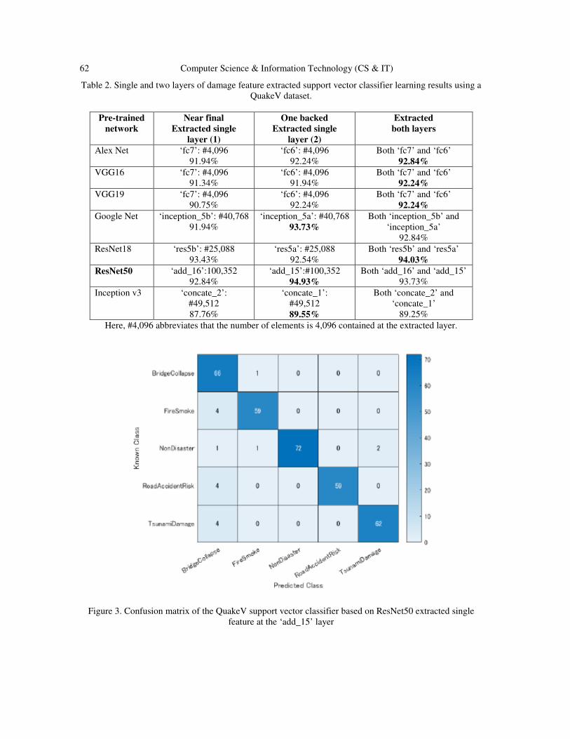
62 Computer Science & Information Technology (CS & IT)
Table 2. Single and two layers of damage feature extracted support vector classifier learning results using a
QuakeV dataset.
Pre-trained
network
Near final
Extracted single
layer (1)
One backed
Extracted single
layer (2)
Extracted
both layers
Alex Net ‘fc7’: #4,096
91.94%
‘fc6’: #4,096
92.24%
Both ‘fc7’ and ‘fc6’
92.84%
VGG16 ‘fc7’: #4,096
91.34%
‘fc6’: #4,096
91.94%
Both ‘fc7’ and ‘fc6’
92.24%
VGG19 ‘fc7’: #4,096
90.75%
‘fc6’: #4,096
92.24%
Both ‘fc7’ and ‘fc6’
92.24%
Google Net ‘inception_5b’: #40,768
91.94%
‘inception_5a’: #40,768
93.73%
Both ‘inception_5b’ and
‘inception_5a’
92.84%
ResNet18 ‘res5b’: #25,088
93.43%
‘res5a’: #25,088
92.54%
Both ‘res5b’ and ‘res5a’
94.03%
ResNet50 ‘add_16’:100,352
92.84%
‘add_15’:#100,352
94.93%
Both ‘add_16’ and ‘add_15’
93.73%
Inception v3 ‘concate_2’:
#49,512
87.76%
‘concate_1’:
#49,512
89.55%
Both ‘concate_2’ and
‘concate_1’
89.25%
Here, #4,096 abbreviates that the number of elements is 4,096 contained at the extracted layer.
Figure 3. Confusion matrix of the QuakeV support vector classifier based on ResNet50 extracted single
feature at the ‘add_15’ layer

Computer Science & Information Technology (CS & IT) 63
Figure 3 shows the confusion matrix of the QuakeV support vector classifier based on the
ResNet50 extracted single feature at the ‘add_15’ layer. Regarding the diagonal value of the
confusion matrix, the predicted labels for each class match almost all the actual disaster feature
classes. In the first row of bridge collapse, there is one false prediction regarding the initial smoke
and fire. In the row for the initial smoke and fire, there are four false predictions related to bridge
collapse. In the row related to non-disaster damage, there are four false predictions related to
bridge collapse, smoke and fire, and tsunami damage. In the row for road damage leading to a
risk of accidents, there are four false predictions related to bridge collapse. Because bridges are
linked to the road network, there are images that fall between bridge collapse and road damage
leading to a risk of accidents, in that there is a view of the road surface in the background. In the
row for tsunami damage, there are four false predictions regarding bridge collapse. Therefore, the
precision of the bridge collapse prediction is lower than that of the other classes. There are certain
cases in which bridges are damaged by a tsunami flow, as occurred in the Great East Japan
Earthquake of 2011. Those predictions were based on one iteration of a five-fold cross validation
classifier. Further hyper-parameter optimization would be required to minimize the prediction
error. Figure 4 shows 15 randomly selected images with the predicted label of the test image
based on the ResNet50 classifier extracted single feature for the ‘add_15’ layer. These predicted
labels are in good agreement with the images of the earthquake damage.
Figure 4. Predicted label of support vector classifier using ResNet50 extracted single feature at the
‘add_15’ layer
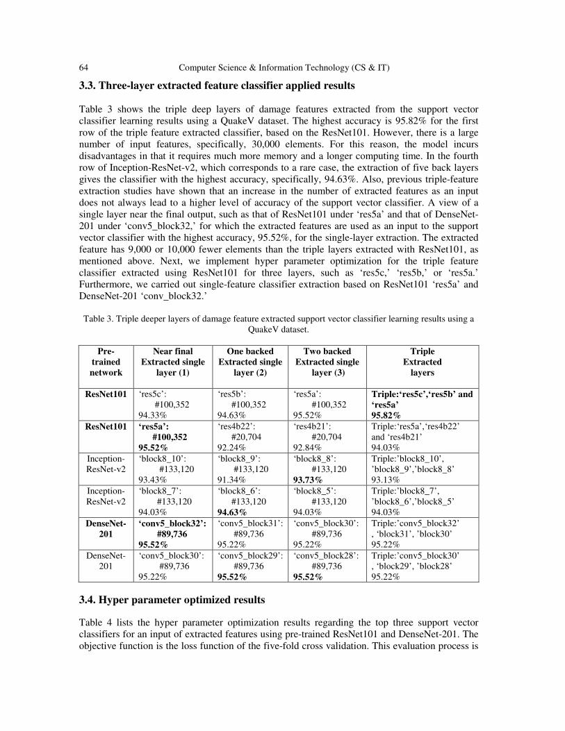
64 Computer Science & Information Technology (CS & IT)
3.3. Three-layer extracted feature classifier applied results
Table 3 shows the triple deep layers of damage features extracted from the support vector
classifier learning results using a QuakeV dataset. The highest accuracy is 95.82% for the first
row of the triple feature extracted classifier, based on the ResNet101. However, there is a large
number of input features, specifically, 30,000 elements. For this reason, the model incurs
disadvantages in that it requires much more memory and a longer computing time. In the fourth
row of Inception-ResNet-v2, which corresponds to a rare case, the extraction of five back layers
gives the classifier with the highest accuracy, specifically, 94.63%. Also, previous triple-feature
extraction studies have shown that an increase in the number of extracted features as an input
does not always lead to a higher level of accuracy of the support vector classifier. A view of a
single layer near the final output, such as that of ResNet101 under ‘res5a’ and that of DenseNet-
201 under ‘conv5_block32,’ for which the extracted features are used as an input to the support
vector classifier with the highest accuracy, 95.52%, for the single-layer extraction. The extracted
feature has 9,000 or 10,000 fewer elements than the triple layers extracted with ResNet101, as
mentioned above. Next, we implement hyper parameter optimization for the triple feature
classifier extracted using ResNet101 for three layers, such as ‘res5c,’ ‘res5b,’ or ‘res5a.’
Furthermore, we carried out single-feature classifier extraction based on ResNet101 ‘res5a’ and
DenseNet-201 ‘conv_block32.’
Table 3. Triple deeper layers of damage feature extracted support vector classifier learning results using a
QuakeV dataset.
Pre-
trained
network
Near final
Extracted single
layer (1)
One backed
Extracted single
layer (2)
Two backed
Extracted single
layer (3)
Triple
Extracted
layers
ResNet101
‘res5c’:
#100,352
94.33%
‘res5b’:
#100,352
94.63%
‘res5a’:
#100,352
95.52%
Triple:‘res5c’,‘res5b’ and
‘res5a’
95.82%
ResNet101
‘res5a’:
#100,352
95.52%
‘res4b22’:
#20,704
92.24%
‘res4b21’:
#20,704
92.84%
Triple:‘res5a’,‘res4b22’
and ‘res4b21’
94.03%
Inception-
ResNet-v2
‘block8_10’:
#133,120
93.43%
‘block8_9’:
#133,120
91.34%
‘block8_8’:
#133,120
93.73%
Triple:’block8_10’,
’block8_9’,’block8_8’
93.13%
Inception-
ResNet-v2
‘block8_7’:
#133,120
94.03%
‘block8_6’:
#133,120
94.63%
‘block8_5’:
#133,120
94.03%
Triple:’block8_7’,
’block8_6’,’block8_5’
94.03%
DenseNet-
201
‘conv5_block32’:
#89,736
95.52%
‘conv5_block31’:
#89,736
95.22%
‘conv5_block30’:
#89,736
95.22%
Triple:’conv5_block32’
, ‘block31’, ’block30’
95.22%
DenseNet-
201
‘conv5_block30’:
#89,736
95.22%
‘conv5_block29’:
#89,736
95.52%
‘conv5_block28’:
#89,736
95.52%
Triple:’conv5_block30’
, ‘block29’, ’block28’
95.22%
3.4. Hyper parameter optimized results
Table 4 lists the hyper parameter optimization results regarding the top three support vector
classifiers for an input of extracted features using pre-trained ResNet101 and DenseNet-201. The
objective function is the loss function of the five-fold cross validation. This evaluation process is

Computer Science & Information Technology (CS & IT) 65
iterated 30 times to minimize the loss. The first row of the table shows the result where the triple
layer features are extracted using ResNet101 under ‘res5c,’ ‘res5b,’ ‘res5a,’ and the feature inputs
are evaluated to optimize the hyper parameters for the support vector classifier, for which the
accuracy is improved to 97.01%, whereas the previously trained value was 95.82%. The
minimum objective function value is 0.0575. Given the large number of feature elements with
three concatenated layers, the evaluation runs took 3.5 h. The second row of the table shows the
results of extracting a single-layer feature using ResNet101 under ‘res5a,’ and for which the
feature input is applied to optimize the hyper parameters for the support vector classifier, for
which the accuracy is improved to 97.50%, whereas the previously trained value was 95.52%.
The minimum objective function value is 0.0627. The training runs took 1.5 h to complete. The
third row of the table shows those results for which the single-layer feature is extracted based on
DenseNet-201 under ‘conv5_block32_concat,’ and the feature input are computed to optimize the
hyper parameters for the support vector classifier, for which the accuracy is improved to 97.50%,
where the previously trained value was 95.52%. This accuracy improvement is the same as that
obtained for the extraction of a single layer with ResNet101. However, the minimum objective
function value is 0.0588. The validation iterations took 1 h, 50 min. Thus, the DenseNet-201-
based feature extraction and hyper parameter optimized support vector classifier are the most
promising when using a QuakeV earthquake damage data.
Table 4. Hyper parameters optimized results of top-3 support vector classifier under an input of extracted
feature using pre-trained ResNet101 and DenseNet-201.
Pre-trained network
Extracted layer trained
classifier
Hyper parameter
optimized classifier
ResNet101
Triple layers
extraction
‘res5c’, ‘res5b’,‘res5a’:
#301,056
95.82%
Objective function : 0.0575
Box constraint C : 0.0061
Rbf kernel scale : 3.0131
Training run time : 215m39s
97.01%
ResNet101
Single layer
extraction
‘res5a’:
#100,352
95.52%
Objective function : 0.0627
Box constraint C : 808.2094
Rbf kernel scale : 625.0391
Training run time : 97m34s
97.50%
DenseNet-201 Single layer
extraction
‘conv5_block32_concat’: #89,736
95.52%
Objective function : 0.0588
Box constraint C : 0.4305
Rbf kernel scale : 0.0649
Training run time : 108m26s
97.50%
Note) The objective function stands for the 5-fold cross validation function value.

66 Computer Science & Information Technology (CS & IT)
Figure 5. Hyper parameters optimization process of support vector classifier based on ResNet101 extracted
single feature ‘res5a’ layer
Figure 5 shows the hyper-parameter optimization process for a support vector classifier based on
the ResNet101 extracted single feature ‘res5a’ layer. After three iterations of five-fold cross
validation, the loss function was minimized at a stable level of around 0.06 during the validation
runs. Furthermore, Figure 6 shows the hyper-parameters optimization process for the support
vector classifier based on the single feature ‘conv5_block32_concat’ layer extracted with
DenseNet-201. After three iterations, the loss function was minimized at a stable level around
0.062. Furthermore, at the points corresponding to six and twelve iterations, the objective
function value was again improved at that point at which the evaluation process converged to a
minimum of 0.058.
Figure 6. Hyper parameters optimization process of support vector classifier based on DenseNet-201
extracted single feature ‘conv5_block32_concat’ layer
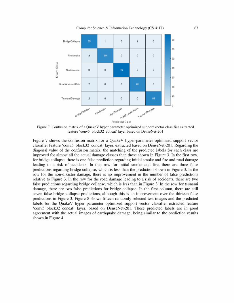
Computer Science & Information Technology (CS & IT) 67
Figure 7. Confusion matrix of a QuakeV hyper parameter optimized support vector classifier extracted
feature ‘conv5_block32_concat’ layer based on DenseNet-201
Figure 7 shows the confusion matrix for a QuakeV hyper-parameter optimized support vector
classifier feature ‘conv5_block32_concat’ layer, extracted based on DenseNet-201. Regarding the
diagonal value of the confusion matrix, the matching of the predicted labels for each class are
improved for almost all the actual damage classes than those shown in Figure 3. In the first row,
for bridge collapse, there is one false prediction regarding initial smoke and fire and road damage
leading to a risk of accidents. In that row for initial smoke and fire, there are three false
predictions regarding bridge collapse, which is less than the prediction shown in Figure 3. In the
row for the non-disaster damage, there is no improvement in the number of false predictions
relative to Figure 3. In the row for the road damage leading to a risk of accidents, there are two
false predictions regarding bridge collapse, which is less than in Figure 3. In the row for tsunami
damage, there are two false predictions for bridge collapse. In the first column, there are still
seven false bridge collapse predictions, although this is an improvement over the thirteen false
predictions in Figure 3. Figure 8 shows fifteen randomly selected test images and the predicted
labels for the QuakeV hyper parameter optimized support vector classifier extracted feature
‘conv5_block32_concat’ layer, based on DenseNet-201. These predicted labels are in good
agreement with the actual images of earthquake damage, being similar to the prediction results
shown in Figure 4.

68 Computer Science & Information Technology (CS & IT)
Figure 8. Predicted label of a QuakeV hyper parameter optimized support vector classifier extracted feature
‘conv5_block32_concat’ layer based on DenseNet-201
4. CONCLUSIONS
To conclude this paper, we present the contribution of this work as demonstrated through several
machine-learning case studies. We believe that disaster damage data mining offers the
opportunity to discover further knowledge needed for disaster mitigation and social loss.
4.1. Contribution of this work
This paper proposes an application to classify disaster damage using feature-extracted support
vector classifiers based on ten pre-trained architectures. These results were applied to a QuakeV
earthquake damage data set. It was found that the disaster damage classifier based on DenseNet-
201 under the single ‘conv5_block32_concat’ layer feature extraction is the most promising with
approximately 97.50% accuracy. Although the ResNet101-based classifier produced the same
level of accuracy, the minimum loss function value is larger than that of the DenseNet-201-based
classifier. To support decision making with respect to the initial response and to mitigate the
relevant loss after a large earthquake using CCTV images, this paper highlighted disaster damage
features such as tsunami damage, bridge collapse, initial smoke and fire, and road damage leading
to a risk of accidents. We actually implemented the image classification method by applying it to
a dataset containing 1,117 images. We drew on relevant open-source websites from which we
could download digital image records of large earthquake damage. Using the ten pre-trained

Computer Science & Information Technology (CS & IT) 69
architectures, we constructed a support vector classification model based on 782 training data sets
and 335 validation images. For one of the feature-extracted learning results, based on ResNet101
and DenseNet-201 using a single layer, we achieved an accuracy of 95.52%. Furthermore, the
hyper parameters of these models could be optimized at an accuracy of 97.50% among our trial
classifiers. After the classification model reads an input image, it can compute the indexes of the
predicted label to determine whether the true disaster feature class belongs to the actual class or
not. Thus, the proposed disaster damage classifier application and the QuakeV earthquake dataset
can be used with datasets consisting of thousands of images.
4.2. Future work
It should be possible to apply disaster damage classification not only to earthquake damage, but
also to other disasters such as building collapse [26], traffic signal failure, landslides, strong
winds [27], and heavy rain and floods [28]. In our daily life, fire and flood disasters occur much
more frequently than earthquakes. This proposed classifier could enable target disaster
surveillance for each region using thousands of disaster feature images covering the target
classes. It would take a long time and a considerable amount of work to collect newly obtained
disaster damage features based on CCTV records and other multi-mode data resources which
contain initial damage features. We will continue to collect video data after a large earthquake
occurs. Disaster datasets are not always learned from overall images, but rather from localized
detections for which the original images focus on clear disaster features. In contrast, the
background disaster region of interest should be excluded for noise reduction. We would monitor
the added variations in the disaster features that have not yet been experienced, such that disaster
damage mining would enable the discovery of the knowledge needed to make decisions on initial
responses with respect to high-priority locations with significantly damaged infrastructure.
ACKNOWLEDGEMENTS
We would like to thank Fukumoto Takuji and Kuramoto Shinichi (MathWorks Japan) for
providing us with useful information on the MATLAB resources such as the Image Processing,
Statistics Machine and Learning, and Deep Learning.
REFERENCES [1] Manzhu, Y., Chaowei, Y., and Yun, L, (2018) Big Data in Natural Disaster Management : A Review,
Geosciences 8, 165.
[2] Michel, U., Thunig, H., Reinartz, P. (2012) Rapid Change Detection Algorithm for Disaster
Management, ISPRS Annals of the Photogrammetry, Remote Sensing and Spatial Information
Sciences, Vol.1-4.
[3] Singh, A. (1989) Review Article Digital Change Detection Techniques using Remotely-sensed data,
International Journal of Remote Sensing, Vol.10, No.6, 989-1003.
[4] Saptarsi, G., Sanjay, C., Sanhita, G. et al. (2016) A Review on Application on Data Mining
Techniques to Combat Natural Disasters, Ain Shams Engineering Journal.
[5] Sakaki, T., Okazaki, M., Matsuo, Y. (2010) Earthquake shakes Twitter users : Real-time Event
Detection by Social Sensors, Proceedings of 19th International Conference on World Wide Web,
ACM.

70 Computer Science & Information Technology (CS & IT)
[6] Walter, D. (1954) Ballantine Books, V-2, ASIN: B000P6L1ES, 14.
[7] SDM (2016) Rise of Surveillance Camera Installed Base Slows,
https://www.sdmmag.com/articles/92407-rise-of-surveillance-camera-installed-base.
[8] Supannee, T., Kurt, T., Sally, E.(2009) Object Oriented Chang Detection of Buildings after a Disaster
ASPRS Annual Conference Baltimore, Maryland.
[9] Ranga, R. Jordan, G. (2012) Probabilistic Change Detection Framework for Analyzing Settlement
Dynamics using Very High-resolution Satellite Imagery, Procedia Computer Science, 9, 907-916.
[10] Maeda, Y., Konno, A, Morita, K. et al. (2018) Infrastructure Disaster Damage Information Real-time
Monitoring, Abstraction, Sharing Techniques Developments, SIP Disaster Prevention Research 2014-
2018, (in Japanese), National Institute for Land and Infrastructure Management (NILIM) Report
2018, 96-97, http://www.nilim.go.jp/english/eindex.htm.
[11] Kataoka, H., Shirakabe, S. et al. (2017) Futuristic Computer Vision through 1,600 papers survey,
CVpaper.challenge in 2016.
[12] National Oceanic and Atmospheric Administration (NOAA), accessed at 2018 Sept 17: Natural
Hazards Image Database, Events contains Earthquake, Tsunami, Volcano, and Geology,
https://www.ngdc.noaa.gov/hazardimages/\#/earthquake.
[13] Aurelien, G. (2017) Hands-On Machine Learning with Scikit-Learn and TensorFlow: Concepts,
Tools, and Techniques to Build Intelligent Systems.
[14] Krizhevsky, A., Ilya S., and G. E. Hinton. (2012) ImageNet Classification with Deep Convolutional
Neural Networks. Advances in neural information processing systems.
[15] Szegedy, C., Wei L., Yangqing J., et al. (2015) Going deeper with convolutions, in Proceedings of the
IEEE conference on computer vision and pattern recognition, 1-9.
[16] VGG model, the Visual Geometry Group at University of Oxford, Simoniyan, K. and Zisserman, A.
(2015) Very Deep Convolutional Networks for Large-Scale Image Recognition, ICLR.
[17] ResNet model, Kaiming, H. Xiangyu, Z., Shaoqing, R. et al. (2015) Deep Residual Learning for
Image Recognition, arXiv:1512.03385v1.
[18] Inception v3 model, Szegedy, C., Vincent, V., Sergey, I. et al. (2015) Rethinking the Inception
Architecture for Computer Vision, CVPR, 2818-2826.
[19] Inception-ResNet-v2 model, Szegedy, C., Sergey, I., Vincent, V. et al. (2016) Inception-v4,
Inception-ResNet and Impact of Residual Connections on Learning, arXiv:1602.07261v2.
[20] DenseNet model, Huang, H., Liu, Z., Maaten, L. et al. (2017) Densely Connected Convolutional
Networks, CVPR.
[21] Hsu C-W., Chang C-C. and Lin C-J. (2003) A Practical Guide to Support Vector Classification,
Technical report, Department of Computer Science, National Taiwan University.
[22] Multi-class classification, pp.29-30, edited by Chan C-C., Lin C-J. (2013) LIBSVM: A Library for
Support Vector Machines, Initial version 2001, Last updated March.

Computer Science & Information Technology (CS & IT) 71
[23] Feurer, M., Klein, A., Eggensperger, K. (2015) Efficient and Robust Automated Machine Learning,
Neural Information Processing Systems Conference (NIPS).
[24] Sibanjan, D., Cakmak, U. M. (2018) Hands-On Automated Machine Learning, Packt.
[25] Gonzalez, R., Woods, R., Eddins, S. (2015) Digital Image Processing Using MATLAB second
edition, McGrawHill Education.
[26] Prince, S. (2017) Computer Vision Models, Learning, and Inference, Cambridge University Press.
[27] Rajalingappaa, S. (2018) Deep Learning for Computer Vision, Packt.
[28] Yasuno, T. (2012) Daily Interaction Behavior, Urgent Support Network on Tohoku Tsunami 2011,
Tottori Quake 2000, Social Capital and Development Trends in Rural Areas Vol.8, Chapter12.
[29] Yasuno, T. (2009) Estimating Occurrence Probability and Loss Index to Manage the Social Risk of
Storong-Winds, International Symposium Society for Social Management Systems(SSMS).
[30] Yasuno, T. (2018) Dam Inflow Time Series Regression Models for Minimizing Loss of Hydro Power
Opportunities, PAKDD Proceedings, the Workshop of Data Mining for Energy Modeling and
Optimisation (DaMEMO) , Melbourne.
AUTHORS
Yasuno Takato received his D.E. degree from Tottori University. He has over 18 years
of consulting engineer experience in infrastructure planning. Now he works proof of
concept (PoC), prototype consulting tool as a senior researcher at the institute (RIIPS)
in Yachiyo Engineering Co., Ltd. His interest is Data Mining and Machine Learning,
Predictive Infrastructure Management, and Time Series Regression. He is a member of
JSAI, ORSJ.
Amakata Masazumi received his B.E degree from Kyoto University and D.E. degree
from Kanazawa University. He has over 20 years of experience in flood control, water
utilization , river environment and he is a specialist of the fluid analysis. Now he works
as a manager of the research institute (RIIPS) in Yachiyo Engineering Co., Ltd. His
research interest is to apply Machine Learning and Deep Learning to the field of civil
engineering.
Fujii Junichiro received his B.E degree from Kyoto University and M.A.S.
(Interdisciplinary Information Studies) degree from University of Tokyo. He has over
15 years of experience in information systems development, and presently works as a
senior researcher at the institute (RIIPS) in Yachiyo Engineering Co., Ltd. His research
interest is applying artificial intelligence to the field of civil engineering.
Shimamoto Yuri recieved her B.E and M.E from Ehime University. She has research
experience in machine learning and image processing, when she is a student concerning
concrete crack. Now she works as a researcher at the institute (RIIPS) in Yachiyo
Engineering Co., Ltd. Her research interest includes Machine Learning and Image
Analysis for civil engineering.

72 Computer Science & Information Technology (CS & IT)
INTENTIONAL BLANK

Natarajan Meghanathan et al. (Eds) : DaKM, SIPP, CCSIT, NCWMC - 2018
pp. 73–83, 2018. © CS & IT-CSCP 2018 DOI : 10.5121/csit.2018.81505
LEARNING TRAJECTORY PATTERNS BY
SEQUENTIAL PATTERN MINING FROM
PROBABILISTIC DATABASES
Josky Aïzan1, Cina Motamed
2 and Eugene C. Ezin
3
1Ecole Doctorale Sciences Exactes et Appliquées
2Laboratoire d’Informatique Signal et Image de la Côte d’OpaleUniversité du
LittoralCôte d’Opale, France 3Institut de Mathématiques et de Sciences Physiques
Université d’Abomey-Calavi, Bénin
ABSTRACT
In this paper, we use Sequential Pattern Mining from Probabilistic Databases to learn
trajectory patterns. Trajectories which are a succession of points are firstly transformed into a
succession of zones by grouping points to build the symbolic sequence database. For each zone
we estimate a confidence level according to the amount of observations appearing during
trajectory in the zone. The management of this confidence allows to reduce efficiently the
volume of useful zones for the learning process. Finally, we applied a Sequential Pattern
Mining algorithm on this probabilistic databases to bring out typical trajectories.
KEYWORDS
Trajectory Patterns, Data Mining, Sequential Pattern Mining, Probabilistic Databases
1. INTRODUCTION
The study of human activities and behaviour is an important research area in computer vision.
Nowadays, automatic activities and behaviour understanding have gained great deal of attention.
Using unsupervised methods, researchers try to observe a scene, learn prototypical activities and
use prototypes for analysis. This approach has been of particular interest for surveillance [1],[2]
and traffic monitoring [3]-[5]where methods for categorizing observed behavior, detecting
abnormal actions for a quick response, and even predicting predict future occurrences are highly
solicited.
Because of large amounts of data in use for these applications, it is difficult to manually analyze
each individually which needs the use of unsupervised methods. In these cases, the data mining in
general and the Sequential Pattern Mining(SPM) in particular appear as promising solutions.
However, it is recognized that data obtained from a wide range of data sources is inherently
uncertain [6], [7]. This paper is concerned with SPM in probabilistic databases [7], a popular
framework for modeling uncertainty and its application to learning trajectory.
This work is organized as follows. In section 2, we present the state of art and related works on
SPM and uncertain SPM. Section 3 describes problem statement while section 4 gives
explanations about learning trajectory with uncertain SPM. Finally, in section 5, we present
experimental results and their analysis. A conclusion ends this work with further directions.

74 Computer Science & Information Technology (CS & IT)
2. STATE OF ART AND RELATED WORKS ON SPM AND UNCERTAIN
SPM
The task of sequential pattern mining consists of discovering interesting subsequences in a set of
sequences. The sequential ordering of events is taken into account unlike pattern mining
introduced by Agrawal and Srikant [8] for finding frequent itemsets. The first sequential pattern
mining algorithm is called AprioriAll [9]. The improved version of this algorithm is Generalized
Sequential Pattern algorithm (GSP) [10]. These two algorithms are inspired by the Apriori
algorithm for frequent itemset mining [8]. GSP algorithm uses a standard database representation,
also called a horizontal database and performs a breadth-first search to discover frequent
sequential patterns. In recent years, other algorithms have been designed to discover sequential
patterns in sequence databases. The Spade algorithm [11] inspired by the Eclat algorithm [12] for
frequent itemset mining, is an alternative algorithm that uses a depth-first search. It uses a vertical
database representation rather than a horizontal database representation. The vertical
representation of a sequence database indicates the itemsets where each item i appears in the
sequence database [11],[13], [14]. For a given item, this information is called the IDList of the
item.
Spam [13] is another algorithm that is an optimization of Spade and also performs a depth-first
search using bit vector IDLists. Recently, the Spam algorithm [13]and Spade algorithm [11] were
improved to obtain the CMSpam and CM- Spade algorithms [14] both based on the observations
that Spam and Spade generate many candidate patterns and perform the join operation to create
the IDList of each of them is costly. Besides depth-first search algorithms and vertical algorithms,
another important type of algorithms for sequential pattern mining is pattern-growth algorithms.
These algorithms are designed to address a limitation of the previously described algorithms,
which is to generate candidate patterns that may not appear in the database.
Uncertainty in SPM can occur in three different aspects: the source (an event is recorded
deterministically, but the source is not readily identifiable), the event (the source of the data is
known, but the events are uncertain) and the time (only time is uncertain) may all be uncertain.
Uncertainty in the time-stamp attribute was considered in [23] and seems not well-suited to the
probabilistic database approach. In this paper, we focus on uncertainty in the source. SPM in
probabilistic databases[7], [6] is a popular framework for modelling uncertainty. Recently several
data mining and ranking problems have been studied in this framework, including top-k [15],
[16], [17] and frequent itemset mining (FIM) [18]-[21]. The SPM problem in probabilistic
databases has been studied in [22]. Also, SPM is studied in noisy sequences [24], but the model
proposed there does not fit in the probabilistic database framework.
3. PROBLEM STATEMENT
3.1. Deterministic SPM
Let� = �1, … , � and = ���, � , … , �� be respectivelya set of sources and a set of items. An
event �is a set of items such that � ⊆ . A sequence database� = ⟨��,� , …,��⟩ is an ordered
list of sequences suchthat each �� ⊆ �is of the form����� , ��, ���, where ����isa unique event-id,
including a time-stamp (events are orderedby this time-stamp), ��is an event and�� is a source.
A sequence is an ordered list of events � = ⟨��, � , … , ��⟩such that �� ⊆ �1 ≤ � ≤ ��. A
sequence � is said to be of length � or a �-sequence if it contains �items, or in otherwords if � = ∑ !�"!�"#� . A sequence �$ = ⟨%�, % , … , %�⟩is a subsequence of another sequence �& =⟨'�, ' , … , '�⟩denoted�$ ≼ �&, if and only if there exist integers 1 < �� < � < ⋯ < �� < +
such that%� ⊆ '��, % ⊆ '� , …, %� ⊆ '��. Let �� = ��|����, �, �� ∈ �be the sequence
corresponding to a source � ordered by ���. For asequence � and source �, let .���, �� be an
indicator variable,whose value is 1 if s is a subsequence of sequence ��, and0otherwise. For any

Computer Science & Information Technology (CS & IT) 75
sequence �, define its support in �, denoted�0���,�� = ∑ .���, ����#� . The goal is to find all
sequences� such that �0���, �� ≥ 2�for some user-defined threshold0 ≤ 2 ≤ 1.
3.2. Source level uncertainty
Proposed by Muzammal and Raman [25], the Source LevelUncertainty (SLU) based on a
probabilistic database �� whichis an ordered list of records ⟨3�, … , 3�⟩such that each3� ∈ �� is of
the form ����, �,4�where ��� is an event-id, � isan event and 4 is a probability distribution over �; the listis ordered by ���. The distribution 4 consists of pairs ��, 5�,where � ∈ � and 0 <5 ≤ 1 is the confidence that the event �is associated with source �; we assume∑ 5�6,7�∈8 =1. An
example can be found in Table 1.
A possible word �∗ of �� is generated by assigning eachevent �� to one of the possible sources �� ∈ 4� .Thusevery record 3� = ����� , �� ,4�� ∈ �� takes the form3:� = ����� , �� , ���in �∗.We
get the complete set of possible words by enumerating all such possible combinations.
Table 1. Source level uncertain database.
eid event W
e1 (a,d) (X:0.6)(Y:0.4)
e2 (a) (Z:1.0)
e3 (a,b) (X:0.3)(Y:0.2)(Z:0.5)
e4 (b,c) (X:0.7)(Z:0.3)
.
Table 2. A database transform to p-sequence.
P-sequence �;� (a, d : 0:6)(a, b : 0:3)(b, c : 0:7) �<� (a, d : 0:4)(a, b : 0:2) �=� (a : 1:0)(a, b : 0:5)(b, c : 0:3)
Pr@�∗A = ∏ C38D��#� @��Ais the probability of a possible word �∗. Forexample, from the database
of Table 1, a possible word �∗can be generated by assigning events ��,�E and �F to .
withprobabilities 0.6,0.3 and 0.7 respectively, and � to K withprobability 1.0. Thus, C3@�∗A =0.6 × 1.0 × 0.3 × 0.7 = 0.126.The support of a sequence in a possible word are well-defined
because every possible word is a (deterministic) database. The definition of the expected support
of a sequence � in ��follows easily:
N���, ��� = O C3@�∗AP∗∈Q8�PR� × �0���, �∗��1� The problem we consider is: Given a probabilistic database��, determine all sequences � such
that N���, ��� ≥ 2+,for some user-specified threshold 2, 0 ≤ 2 ≤ 1. Since thereare potentially
an exponential number of possible words, it isinfeasible to compute N���, ��� directly using
Equation 1.Next,we show how to do this computation more efficiently.
3.3. Computing Expected Support
A sequence of the form⟨���, 5��, … , ���, 5��⟩, where �" isan event and 5"is a confidence value is
called p-sequence.It’s analogous to a source sequence in classical SPM. For examples, we write a
p-sequence ⟨��S, T, 0.3�, ��T, 5, 0.7�⟩as�S, T: 0.3��T, 5: 0.7�.An SLU database ��is as
acollection of p-sequences��Q , … , ��Q , where ��Q is the p-sequence of source �, and contains a list
of pairs ���, 5�� with1 ≤ � ≤ �, where ��are those events in ��that have nonzeroconfidence of
being assigned to source �, ordered by��� (see Table 2). However, the p-sequences corresponding

76 Computer Science & Information Technology (CS & IT)
to different sources are not independent. Thus, one may view an SLU event database as a
collection of p-sequences with dependencies in the form of x-tuples [26]. Nevertheless,
Muzammal and Raman [25] showed that we can still process the p-sequences independently for
the purposes of expected support computation: N���, ��� = O C3@�∗AP∗∈Q8�PR� × �0���, �∗�
= OC3@�∗AP∗ ×O.���, �∗���#�
= OOC3@�∗A ×P∗��#� .���, �∗�
= ON@.���, ���A��#�
�2�
where N denotes the expected value of a random variable.Since .� is a 0 − 1 variable, N@.���, ���A = C3W� ≼ ���X, andwe calculate the right-hand expression, which refer to as the
source support probability.
Computing the Source Support Probability. Given ap-sequence ��� = ⟨���, 5��,… , ��Y , 5Y�⟩ and a sequence� = ⟨��,� , …,�Z⟩, a �[ + 1� ×�3 + 1� matrix %�,]@0. . [A@0. . 3Ais created
(the subscripts on A are omitted when the sourceand sequence are clear from the context). For 1 ≤ � ≤ [and 1 ≤ ^ ≤ 3, %@�, ^A will containC3@⟨��, … , ��⟩ ≼ ⟨���, 5��,… , ��_, 5_�⟩A. Set %@0, ^A = 1 for all ^,0 ≤ ^ ≤ 3and %@�, 0A = 0 for all 1 ≤ � ≤ [, and compute the
othervalues row-by-row. For 1 ≤ � ≤ [ and 1 ≤ ^ ≤ 3, define:
`�,_∗ =a _̀ �b�� ⊆ �_0cdℎ�3f���
g �3�
The interpretation of Equation 3is that `�,_∗ is the probability that�_ allows the element ��to be
matched in source �; this is 0if �� ⊈ �_, and is otherwise equal to the probability that �_ isassociated with source �. Now Equation 4 is used. %@�, ^A = j1 − `�,_∗ k × %@�, ^ − 1A + `�,_∗ × %@� − 1, ^ − 1A.�4�
Table 3 shows the computation of the source support probability of sequence � = �S��T� for
source . in theprobabilistic database of Table 1. Similarly, we can compute C3@� ≼ �<�A = 0.08 and C3@� ≼ �=�A = 0.35. So, the expected support of (a)(b) in the
database of Table 1 is0.558 + 0.08 + 0.35 = 1.288.
The reason Equation 3is correct is that if �� ⊈ �_ then theprobability that⟨��, … , ��⟩ ≼⟨��, … , �_⟩ is the same asthe probability that ⟨��, … , ��⟩ ≼ ⟨��, … , �_n�⟩(note that if �� ⊈ �_ then `�,_∗ = 0and %@�, ^A = %@�, ^ − 1A). Otherwise,`�,_∗ = _̀ and two disjoint sets of possible words
have to beconsidered: those where �_ is not associated with source � (thefirst term in Equation 3)
and those where it is (the second term in Equation 3). In summary, given a p-sequence ���and a
sequence �,by applying Equation 3repeatedly, C3W� ≼ ���X, is correctly computed.

Computer Science & Information Technology (CS & IT)
4. LEARNING TRAJECTORY The types of sequential data commonly used in data mining
time-series is an ordered list of numbers, while a
(symbols). The problem of sequential pattern mining
sequences [10].However, it can also be applied to time
sequences using discretization techniques.
To build the database of sequences we used a database
succession of points�., o� in pixel.
Figure 1. Illustration of trajectory sequence
Trajectories are transformed into a sequence
sequence database. For example,
coordinates belong to the interval
belongto the interval A50, 100@ belong to the interval @0, 50A aregrouped in zone
theinterval A50, 100@ are grouped in Zone
in zone %2 and a coordinatepoint
trajectory crossing a zone, a symbol linked to the zoneis generated and a confidence (uncertainty)
level is estimatedbased on the number of
the uncertainty of the symbol linked to this
uncertain symbols (see Figure 1).
Computer Science & Information Technology (CS & IT)
RAJECTORY WITH UNCERTAIN SPM
The types of sequential data commonly used in data mining are time-series and sequences [27]. A
list of numbers, while a sequence is an ordered list of nominal
(symbols). The problem of sequential pattern mining was originally designed to be applied to
sequences [10].However, it can also be applied to time-series after converting time
ization techniques.
To build the database of sequences we used a database where trajectories are represented by a
in pixel.
Illustration of trajectory sequence (D6D5D4D3D2E2F2)with the confidence of the symbol
Trajectories are transformed into a sequence of zones by grouping points to build the symbolic
example, if we consider intervals of 50 pixels,the points whose
coordinates belong to the interval @0, 50Aare grouped in zone %. Those whose . are grouped in zone ' and so on.Points whose oaregrouped in zone 1. Those whose o -coordinates belong to
are grouped in Zone 2 and so on. Therefore,a coordinate point
and a coordinatepoint �100, 50� is in zone '1 (see Figure4 and Figure
trajectory crossing a zone, a symbol linked to the zoneis generated and a confidence (uncertainty)
is estimatedbased on the number of points inside the zone. The confidence level represents
the uncertainty of the symbol linked to this zone. This allows to generate the sequences with
1).
77
series and sequences [27]. A
sequence is an ordered list of nominal values
was originally designed to be applied to
time-series to
where trajectories are represented by a
with the confidence of the symbols
of zones by grouping points to build the symbolic
pixels,the points whose .-.-coordinates o -coordinates
coordinates belong to
and so on. Therefore,a coordinate point �50, 100� is
ure5). Foreach
trajectory crossing a zone, a symbol linked to the zoneis generated and a confidence (uncertainty)
level represents
zone. This allows to generate the sequences with

78 Computer Science & Information Technology (CS & IT)
5. SIMULATION RESULTS AND DISCUSSIONS
In this section, we present the results we obtained in our work. We choose the CVRR Trajectory
Clustering Dataset [28]for benchmarking trajectory clustering algorithms.
Figure 2. Cross trajectory dataset
Figure 3. Labomni trajectory dataset
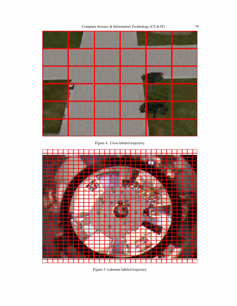
Computer Science & Information Technology (CS & IT)
Figure 5. Labomni labeled trajectory
Computer Science & Information Technology (CS & IT)
Figure 4. Cross labeled trajectory
Figure 5. Labomni labeled trajectory
79

80 Computer Science & Information Technology (CS & IT)
Table 3. Computing of the source support probability.
�S, �: 0.6� �S, T: 0.3� �T, 5: 0.7� �S� 0.4 × 0 + 0.6 × 1 = 0.6 0.7 × 0.6 + 0.3 × 1 = 0.72 0.72 �S��T� 0 0.7 × 0 + 0.3 × 0.6 = 0.18 0.3 × 0.18 + 0.7 × 0.72 = 0.558
5.1. CVRR trajectory clustering dataset
The full dataset of trajectory similarity/distance measures and clustering algorithms. In our case,
we use CROSS (Figure 2) and LABOMNI (Figure 3) dataset.
The CROSS dataset contains a four way traffic intersection. Units are pixels.
The LABOMNI dataset examines humans rather than vehicles. An omni-directional camera was
placed in the middle of a lab to observe trajectories from a less constrained environment than
encountered by vehicle traffic. The participants were not aware of the data collection to ensure
naturally occurring motion patterns. The trajectories have a long time duration and tend to have a
large degree of overlap in the image plane. Units are pixels.
Table 4. Results of deterministic SPM and uncertain SPM.
Dataset SPM frequent
patterns
Uncertain SPM frequent
patterns
Unreliable
frequent patterns
rate (%)
Reliable
frequent
patterns rate
(%)
Cross 152 67 56% 44%
Labomni 31 17 45% 55%
5.2. Results and discussions
Our implementation in Java, is executed on a machine Intel(R) Core(TM) i7-7500U CPU @2.70
GHZ 2.90 GHZ running Windows 10. With a support value fixed to0.05, thedifferent results
obtain are in Table 4.
With Cross dataset, there are 152 frequent sequences (obtainedwith deterministic database) of
which 85 are consideredunreliable, or a rate of 56% (obtained with the probabilistic database).
With Labomni dataset, unlike in the case of Crossdataset, the unreliable frequent sequence rate �45%� is lowerthan the reliable frequent sequence rate.
It is noted from the results that in the two datasets used, the unreliable frequent sequence patterns
rate is not equal to0%. This result leads us to say that the deterministic SPM returns frequent
sequences patterns that are not necessarily all reliable and justifies our choice on the uncertain
SPM.
The results also show that the unreliable frequent sequence patterns rate of the Cross dataset is
higher than that of the Labomni dataset. This could be explained by the fact that the data of the
Labomni dataset are taken in an environment with less constraint than that of the Cross dataset
where vehicle traffic is observed.
6. CONCLUSIONS
We have adapted a Sequential Pattern Mining algorithm for probabilistic databases to bring out
typical trajectories. The management of the uncertainty of data help to focus on reliable part of
the data. By using symbols with their uncertainties, the system estimates reliable frequent
trajectory models by using the Sequential Pattern Mining algorithm.

Computer Science & Information Technology (CS & IT) 81
For the future work, two possible extensions will be studied .The first one is the integration of
temporal constraints (including the time uncertainty management) and the second extension is on
the development of an online recognition system of sequential patterns in the context of uncertain
observation and models.
REFERENCES
[1] C. Stauffer and W. E. L. Grimson, Learning patterns of activity usingreal-time tracking, IEEE Trans.
Pattern Anal. Mach. Intell., vol. 22, no.8, pp. 747757, Aug. 2000.
[2] D. Makris and T. Ellis, Learning semantic scene models from observingactivity in visual surveillance,
IEEE Trans. Syst., Man, Cybern. B, vol.35, no. 3, pp. 397408, Jun. 2005.
[3] C. Piciarelli and G. L. Foresti, On-line trajectory clustering for anomalousevents detection, Pattern
Recognition Letters, vol. 27, no. 15, pp.18351842, Nov. 2006.
[4] S. Atev, O. Masoud, and N. Papanikolopoulos, Learning traffic patternsat intersections by spectral
clustering of motion trajectories, inIEEE Conf. Intell. Robots and Systems, Bejing, China,
pp.48514856, Oct. 2006.
[5] B. T. Morris and M. M. Trivedi, Learning, modeling, and classificationof vehicle track patterns from
live video, IEEE Trans. Intell. Transp.Syst., vol. 9, no. 3, pp. 425437, Sep. 2008.
[6] Aggarwal, C.C. (ed.): Managing and Mining Uncertain Data. Springer2009.
[7] Suciu, D., Dalvi, N.N.: Foundations of probabilistic answers to queries.In: Ozcan, F. (ed.) SIGMOD
Conference. p. 963. ACM 2005.
[8] R. Agrawal and R. Srikant, Fast algorithms for mining association rules,The International Conference
on Very Large Databases, pp. 487-499,1994.
[9] R. Agrawal, and R. Srikant, Mining sequential patterns, The InternationalConference on Data
Engineering, pp. 3-14, 1995.
[10] R. Srikant, and R. Agrawal, Mining sequential patterns: Generalizationsand performance
improvements, The International Conference on ExtendingDatabase Technology, pp. 1-17, 1996.
[11] M. J. Zaki, SPADE: An effcient algorithm for mining frequent sequences,Machine learning, vol.
42(1-2), pp. 31-60, 2001.
[12] M. J. Zaki, Scalable algorithms for association mining, IEEE Transactionson Knowledge and Data
Engineering, vol. 12(3), pp. 372-390,2000.
[13] J. Ayres, J. Flannick, J. Gehrke, and T. Yiu, Sequential pattern miningusing a bitmap representation,
ACM SIGKDD International Conferenceon Knowledge Discovery and Data Mining, pp. 429-435,
2002.
[14] P. Fournier-Viger, A. Gomariz, M. Campos, and R. Thomas, Fast VerticalMining of Sequential
Patterns Using Co-occurrence Information, ThePacic-Asia Conference on KnowledgeDiscovery and
Data Mining, pp. 40-52, 2014.
[15] Hua, M., Pei, J., Zhang, W., Lin, X.: Ranking queries on uncertain data:a probabilistic threshold
approach. In: Wang [21], pp. 673686.
[16] Zhang, Q., Li, F., Yi, K.: Finding frequent items in probabilistic data.In: Wang[21], pp. 819832.

82 Computer Science & Information Technology (CS & IT)
[17] Cormode, G., Li, F., Yi, K.: Semantics of ranking queries for probabilisticdata and expected ranks. In:
ICDE. pp. 305316. IEEE 2009.
[18] Aggarwal, C.C., Li, Y.,Wang, J.,Wang, J.: Frequent pattern mining withuncertain data. In: Elder et al.
[9], pp. 2938.
[19] Bernecker, T., Kriegel, H.P., Renz, M., Verhein, F., Zufle, A.: Probabilisticfrequent itemset mining in
uncertain databases. In: Elder et al.[9], pp. 119128.
[20] Chui, C.K., Kao, B.: A decremental approach for mining frequentitemsets from uncertain data. In:
PAKDD. pp. 6475 2008.
[21] Chui, C.K., Kao, B., Hung, E.: Mining frequent itemsets from uncertaindata. In: Zhou, Z.H., Li, H.,
Yang, Q. (eds.) PAKDD. LNCS, vol. 4426,pp. 4758. Springer 2007.
[22] Muzammal, M., Raman, R.: On probabilistic models for uncertainsequential pattern mining. In: Cao,
L., Feng, Y., Zhong, J. (eds.) ADMA(1). LNCS, vol. 6440, pp. 6072. Springer 2010.
[23] Sun, X., Orlowska, M.E., Li, X.: Introducing uncertainty into patterndiscovery in temporalevent
sequences. In: ICDM. pp. 299306. IEEEComputer Society 2003.
[24] Yang, J., Wang, W., Yu, P.S., Han, J.: Mining long sequential patterns ina noisy environment. In:
Franklin, M.J., Moon, B., Ailamaki, A. (eds.)SIGMOD Conference. pp. 406417. ACM 2002.
[25] M. Muzammal, and R. Raman, ”Mining sequential patterns from probabilisticdatabases,” Knowledge
and Information Systems, vol. 44(2), pp.325-358, 2015.
[26] Cormode, G., Li, F., Yi, K.: Semantics of ranking queries for probabilisticdata and expected ranks. In:
ICDE. pp. 305316. IEEE 2009.
[27] J. Han, J. Pei, and M. Kamber, Data mining: concepts and techniques, Amsterdam:Elsevier 2011.
[28] B. T. Morris and M. M. Trivedi, Learning Trajectory Patterns by Clustering: Experimental Studies
and Comparative Evaluation, in Proc.IEEE Inter. Conf. on Computer Vision and Pattern Recog.,
Maimi,Florida, June. 2009.
AUTHORS
Josky Aïzan received a Bachelor Engineering degree from Ecole Nationale
d’Economie Appliquée et de Management of Université d’Abomey-Calavi, Bénin in
2004 and Master degree in Computer Engineering in 2016 from Institut de Formation
et de Recherche en Informatique of Université d’Abomey-Calavi, Bénin. He is
currently a Ph.D student in Computer Engineering at Ecole Doctorale Sciences
Exactes et Appliquées of Université d’Abomey-Calavi, Bénin and at Université du
Littoral Côte d’Opale, France. His research interests include signal processing, image
processing, video processing, machine learning and pattern analysis and recognition.
Cina Motamed is associate professor in Computer Science in the University of Littoral
Cote d’Opale, Calais, France. He received his B.Sc. in mathematics, and M.Sc in
Electrical Engineering and Computer Science from the University of Caen, France and
the PhD degree in Computer Science from the University of Compiegne, France, in
1987, 1989, and 1992, respectively. Current research is concerned with the automatic
visual surveillance of wide area scenes using computational vision. His research
interests focus on the design of multicamera system for real-time multiobject tracking
and human action recognition. He is recently focusing on the uncertainty management
over the vision system by using graphical models, and beliefs propagation.He is also
interested by unsupervised learning approaches for human activity recognition.

Computer Science & Information Technology (CS & IT) 83
Eugene C. Ezin is a Full Professor in Computer science and Artificial Intelligence. He
received his PhD degree with highest level of distinction in 2001 after research works
carried out on neural networks and neural fuzzy systems for speech applications at the
International Institute for Advanced Scientific Studies in Italy. He is a reviewer of
many conferences and journals. His research interests include machine learning,
expert systems, signal and image processing, high performance computing,
cryptography, information systems and network security.

84 Computer Science & Information Technology (CS & IT)
INTENTIONAL BLANK

Natarajan Meghanathan et al. (Eds) : DaKM, SIPP, CCSIT, NCWMC - 2018
pp. 85–97, 2018. © CS & IT-CSCP 2018 DOI : 10.5121/csit.2018.81506
AN INTELLIGENT APPROACH OF THE
FISH FEEDING SYSTEM
Mohammed M. Alammar and Ali Al-Ataby.
Department of Electrical Engineering and Electronics,
University of Liverpool, Liverpool, United Kingdom
ABSTRACT
Fish breeding is a promising branch of farming, so the creation of tools for automation of this
area is quite relevant. Feeding on fish farms is the main component of the successful functioning
of such businesses. However, this process requires an in-depth preparation, as each species of
fish has a different food culture, as well as various behaviours during nutrition. Moreover, in
the method of feeding fish, farmers must take into account the age, size of the fish, and other
characteristics. This paper contains information on the creation of a Preference testing by
images processing is considered as the most effective tool that can be used to determine the
sensory behaviour of an animal, which can record the eating behaviour of fish and determine
the degree of their hunger, and, finally, to feed them. Moreover, small fish are shyer, which
provokes their malnutrition. A smart feeding system can solve the issue of uniform the
distribution of food for all fishes.
KEYWORDS
Fish Feeding, Preference testing, Fish Farming, Smart Feeding System, Methods of Fish
Feeding.
1. INTRODUCTION Fish farming is perspective business, which grows rapidly as it is shown in the (Fig.1). Indeed,
fish feeding is one of the crucial forms of intensification of the fish-farming process [1]. Correct
fish feeding in farming allows applying more dense plantings, and, thereby, increasing the fish
productivity of ponds.
Figure 1. World fish production from 1950 to 2014 [2]

86 Computer Science & Information Technology (CS & IT)
Currently, fisheries around the world try to use various artificial food additives, which include all
the substances necessary for the healthy growth and development of fish [1]. Feeding the fish is
based on natural food, which the fish can usually find in natural water reservoirs, but on farms,
this food contains more vitamins and other nutrients (Table 1) [3].
Additionally, aquaculture is the cultivation of fish and crayfishes in the closed-cycle systems [4].
Like any business or occupation, aquaculture can face many risks and challenges. Aquaculture
makes it possible to grow living organisms in small volumes in conditions as close as possible to
natural ones. The task of any aqua-farmer is to create such conditions in which the fish can
behave comfortable and grow fast. Indeed, such growth is possible only in conditions, which are
as close to natural ones as possible, and include rational feeding of all species of fish, regardless
of their size and activity. More often, the natural habitat of a particular type of fish is in a much
worse form, including drying up and salinization of water bodies, and pollution with industrial
wastes. All this affects the natural habitat of fish. Finally, the task of the farmer is to create such
conditions that the fish would feel comfortable for reproduction.
Table 1. The types of food of fish on farms [3]
An intelligent feeding system is a quite simple and low cost which will motivate the fish farmers
to acquire it. Moreover, the system can reports will convey information about the number and size
of fish and their behaviour. Indicators will contain information about such categories of fish as
small, medium and large ones. Based on the analysis of the size of fish and their behaviour, the
farmer can draw conclusions about the correlation between these two indicators. However, an
intelligent feeding system can reduce the amount of used feed by 20% [5]. However, a false
positive rate, which detects hungry fish without reasons, can feed the fished when they are full.
The percentage of damage from such false feeding is not fully researched. This system will
provide the estimation of the preference fish feeding by using efficient ways can observe fish
behaviour and response with feeding which is significant for the farmers to improve fish
production in a short period of time and at low cost.
2. LITERATURE REVIEW
Fish farming has gained traction in recent years due to depleting stocks in the ocean that have
forced people to rear marine life in a domesticated environment. However, feeding has become a
challenge since vast amounts of food are wasted that may lead to water toxicity. In any case,
manual feeding is not efficiently leading to high operational costs. Development of an automatic
feeding system is highly advised since it enables a farmer to automate the process thus enhancing
efficiency. The Sustainable Aquaculture Feed System is a useful digital device that can identify

Computer Science & Information Technology (CS & IT) 87
fish species, sex, and count, which enables the farmer to develop a feeding program. Broadly, the
automation of fish feeding systems is bound to improve efficiency in aquaculture farms.
2.1 Review of Automatic Fish Feeding Techniques
Fish farming is a multi-billion industry that has evolved to incorporate technology into the
management that includes smart feeding systems. Towards this end, a comparison of several
feeding systems is vital to establish the operating mechanisms of the structures under review. To
begin with, the Sustainable Aquaculture Feed System has been equipped with a vision sensor
machine that is used to estimate the amount of feed required by the livestock being reared, which
prevents waste of nutrients availed to the fish [6]. Notably, the system can count the number of
fish that is critical in determining the amount of food required by the fish. In relation, the
technology can be used to deduce the size of the fish, which is essential in formulating the
feeding program to ensure that the amount released is sufficient. Even further, the approach can
detect the gender of the marine species since they require different nutritional amounts.
Finally, the model can be used to identify the type of fish in the farm, which is used to inform the
feeding program. The system has employed the bio-scanner to undertake the requirements as
mentioned above with considerable success. The SAFS system has several components that
include both hardware and software processing elements, which include a camera, Bluetooth
receiver, and input devices. The hardware part consists of a camera, sensors, and the feeder
system [6]. The incorporation of a graphical user interface is essential since it provides data
analysis structure that is used to study patterns in the tanks [7]. The use of Bluetooth is designed
to ensure information is relayed to the required area electronically, which allows that graphic
images can be shared within system components. The inclusion of a timer is critical to the success
of the feeding system since it ensures the fish are fed at the appropriate time with the video
having three frames image per second.
On the other hand, the development of an automatic feeder system has led to the creation of a
smart system, which is controlled using artificial intelligence. The idea is to monitor the feeding
process continuously utilising the interface. The device uses the Global Standard for Mobile
Communication, which enables the firm to track the progress of the feeding program remotely
[8]. Ideally, the invention is applied to issue commands to the feeding program in real-time.
Consequently, the system can operate with minimal human intervention resulting in a fully
automated product. The inclusion of a central processing unit is essential since it receives all
inputs in the system that is processed before being used to issue commands in the smart feeding
program. The system has a temperature sensor, which is used to analyse the conditions in the
water. It is imperative to state that water heat is critical in aquaculture since it influences the
deterioration of either the feed, which might affect positively or negatively the nutritional content.
The inclusion of a camera is designed to ensure digital images of the fish stock can be monitored
using the structure [9]. The camera enables the farmer to identify the number of fish, sex, size,
and number, which inform the amount and type of feed to be released into the farm. In fact, the
system has an 80% accuracy, which is good considering that the smart feeding industry is
relatively nascent. Being able to deduce the physical characteristics of the fish enables the farmer
to release the correct amount of feed, which reduces wastage, especially in controlled
aquaculture. Time management is another vital element that has been considered in the design
since the fish stock must be fed at appropriate times to ensure optimal nutritional value is derived
from the feeds.

88 Computer Science & Information Technology (CS & IT)
Table 2. Comparison of Different Fish Feeding System
The use of Automatic Computer Vision Systems for Aquatic Research is an efficient system that
has been developed to facilitate feeding of fish. The structure addresses several critical issues,
which include the incorporation of a sizing mechanism that can be used to inform the amount of
feed to be released into the farm. Further, the identification of fish species, specifically the zebra
fish is another critical component of the system that determines the type of feeds to be used in
feeding the marine animal. Again, the automated system enables the farmer to analyse the
behaviour of larval fish in the farm, which can deduce trends and patterns that can be used to
develop a feeding program. The system is equipped with a camera and computer processing
facility that can produce information [10].
In summation, depleting fish stocks in the ocean have led to the development of aquaculture
farms that require substantial amounts of feeds. The creation of fish feeding systems been
automated to ensure the process is efficient. Notably, manual feeding is wasteful and unable to
detect the nutritional needs of marine animals rightly. The Solar Powered Automatic Shrimp
Feeding System has integrated several components that ensure shrimps are fed at specific
intervals. The structure uses solar energy to release food into the tank, which improves energy
efficiency. To conclude, the automation of a feeding system in fish farms will enhance the
productivity of the products.
2.2 Challenges and Opportunities
The principal risks of aqua farming are fish diseases, technical malfunctions in the work of
equipment for feeding fish, saturation of water with oxygen, substandard feed, and others [12].
Additionally, usually, the feeding of fish is between 50% and 80 % of the overhead costs of a fish
farm [12]. Nutrition is a manual task, so it is an immeasurable and inaccurate method with such
results as overfeeding and underfeeding of fish. Overfeeding means that the majority of food goes
to waste, and it infringes the financial part of aqua farming, the surrounding the farm marine
environment, and the health of the fish. On the other hand, the lack of feeding leads to famine and
the gradual dying of fish. Moreover, some challenges may be faced with the course of this
project. These challenges may include:
1. Fish Size: Fish of various sizes take food differently. Small fish are more passive in the fight
for food because of their size, so they get insufficient food. Indeed, many fish are shy, and
they are at a far distance from the bold fish, which get food together. Shy fish receive an
inadequate amount of food, therefore, improving the method of feeding fish is a critical point
in the successful operation of aqua farms. The development of an automatic intelligent
feeding system is significant for solving these problems and distributing the right amount of
feed using sensors that measure the appetite of fish.
Nutrition and feeding have a significant effect on the health of fish. It affects their behaviour
and response to different environmental conditions. Since fish of different size have different
Market Sizing Feeding Analysis Tracking
Automatic Computer Vision Systems for Aquatic
Research[10]
Yes Yes Yes
Sustainable Aquaculture Feed System [6] Yes Yes Yes Yes
The Automatic Feeder System [8] Yes Yes Yes Yes
Solar Powered Automatic Shrimp Feeding System [11] Yes

Computer Science & Information Technology (CS & IT) 89
feeding patterns, it is prudent to learn their behaviour which helps the farmer to prepare an
effective fishing schedule. According to Lall and Tibbetts, fish behave differently depending
on the feeding habit, feeding method as well as the frequency of feeding [13]. The proposed
system will be able to analyse the food preference of a shoal for optimal growth.
2. Fish Behaviours: The behaviour of fish associated with nutrition depends on their type, size,
and sometimes on their sex [1]. Fishes usually eat other fishes or plants. Even representatives
of fish species, which do not belong to predators, eat small fish when their size is equal to the
preferred food. Indeed, adult fish mostly eat caviar and fry if they find it in the nearest area.
Moreover, fishes use to dig in the ground. Some fish directly get their own food in the
uppermost layer of soil, while others sift the ground through the gills and during this process
sometimes absorb reasonably large pieces of soil.
According to Lovell, of all the spectrum of behavioural reactions manifested by fish, the main
one is the behaviour associated with nutrition [1]. Food behaviour is a complicated process of
a successive change of individual behavioural phases and acts from the moment of obtaining
information about the presence in the environment of food objects before deciding whether to
seize or reject them [1]. The first phase of the nutrition behaviour of fish is the rest, which is
such state of fish when it does not react to the external food stimuli. It is common for the
majority of species, and it happens due to various causes, including illness, the closeness of
spawning period, wintering, etc. The second phase is the readiness for obtaining the signal on
food availability. The third phase is an obtaining signal on food availability. In the process of
scanning the water reservoir, the fish eventually discovers the signal emanating from the food
object. In the process, all sensory systems of fish are involved, so the signs received can be
variable in nature and have different intensity and direction. The next phase is the search and
detection of the source of food. Therefore, among the whole spectrum of available signals,
the fish chooses one. After the food signal is selected, fish start to search for the source. The
last phase is the determination of the suitability of food.
Moreover, Abdallah and Elmessery have stated that some fish used to eat only in open spaces
[14]. Others, which are shyer, hide in the clefts anticipating the best moment to swim out.
Cereal fishes spend a very long time feeding to satisfy their nutritional needs, while predatory
species like eels are not eaten every day. These varied ways of feeding become apparent in
the artificial ponds and require attention. Otherwise, the fish will not survive. Indeed, small
fish may not receive enough feed because they have shy behaviour patterns. According to
Abdallah and Elmessery, small fish may not appear near the sensors of hunger control, so
they may remain hungry, and would have to eat a minimum amount of snacks after huge
fishes [14]. Moreover, AlZubi thinks that this intelligent system of feeding fish requires the
significant campaign of advertisement and popularisation, since the majority of farmers are
not accustomed to the idea of using technology in their production process [5]. In the
beginning, many of them were resistant to adopting the application, but education and
training, as well as a rental system, allowed them to spend less money and give them the real
evidence [5].
3. Fish Tracking: According to Al-Jubouri, the current fish tracking methods require the tagging
of an individual fish which is quite challenging [10]. This calls for the need of advanced
system whereby the non-contact method of recognising a particular free moving fish has been
developed. The system does not only reduce the time for tagging process but also offer a real-
time recognition technique. The computer-aided tool in its different models provides a
successful solution for analysing the behaviour of fish, their feeding habit, and size. Studies
to find out whether fish have the capacity painful stimuli and associated discomfort have been
faced with a challenge of ethical restriction. Larval zebra has been used instead since their
responses are similar to those of the adults. It is therefore advisable to consider the ethical

90 Computer Science & Information Technology (CS & IT)
suitability of a given system that affects the behaviour of fish or any other animal being used
in the study.
3. AIMS AND OBJECTIVES
The system should accomplish the task in three stages. The first stage in the algorithm is the
object detection where the subject under the study is identified. The object is then tracked and
monitored closely where the activities are recorded. For this case, a fish will be identified and
monitored. The collected data is processed and a conclusion drawn from the analysis. Three
stimulation techniques can be used in the study; they include thermal, electrical and chemical
stimulation. Electrical stimulation is the most opposed technique among the three since it inflicts
pain on the object under study. It is therefore used in a limited number of studies.it is also
associated with unpredictable behavioural reactions. It is also not easy to capture the movement
of small fish with this method due to the transparency in their body [10].
3.1 The Aims of This Study
In this study, to achieve the aims of study the system smart fish feeding. This will encompass:
1. In order to precisely identify and measure the amount of feed for each fish
2. Minimising the impact of traditional feeding mechanisms
3. Testing the fish preference for type of feed
4. Minimising the feed waste and maximising the conversion rate of food products
3.2 Objectives
The Objectives of the project can be defined as:
1. Optimising diet for fish
2. Developing a new way to keep the fish tank clean
3. Developing new ways of modulating data onto a smart fish feeding system
4. Determining the possibilities of feeding fish system recreation using digital data
4. EXPECTED MATERIALS AND METHODS
4.1 Design considerations
This project will provide the estimation of the preference fish feeding by using ways to observe
fish behaviour and response to the type of feed. This project require tank is separated into two
areas; Living Area and Feeding Area which is the diet area. Living Area that is comfortable to
fish contains gravel and plants, however, Feeding Area is less comfortable because it is less
natural and bare to fish (Fig.2). The design shows the recirculation system which consists of a
water filter and pump that is used for filtration and measure the amount of waste of feed.
Furthermore, the sensors may not always fully reflect the state of the fish. Many water parameters
should be measured: pH, the temperature, salinity, dissolved oxygen, ammonium, the
transparency, the suspended solids, nitrates, the total nitrogen or match soluble reagent, among
others [15]. The smart fish feeding architecture comprises of a few components, which includes
the hardware design, and the software algorithm with the database of the fish.

Computer Science & Information Technology (CS & IT) 91
Figure 2. The smart fish feeding system setup
4.2 Methodology
Modern methods of fish feeding include an intelligent feeding system based on fish behaviour
and extend to speed respond fishes toward one kind of feed to minimise the impact of traditional
feeding mechanisms. The proposed mechanism of nutrition interacts, recognises and reacts to the
activity of fish [5]. Such feeding system feeds fish at their request, regardless of the time of the
day. Figure 3, shows the block diagram of the system measure the Feeding Efficiency (FE), and
Specific Growth Rate (SGR, % body weight per day) which reflects fish respond development of
the given feed.
Figure 3: Block diagram of the proposed system
Where N number of tanks fish feeding which each tank feeding by one type of different feed. The
system connects to each tank that has the same volume of feed. The system could study the
preference testing for fish. Moreover, this design system is used to study the behaviour and
growth of fish toward a certain food. First of all, assume the fish does not have any knowledge
about the new fish feeding mechanism. In order to introduce the system to fish, the food is
dispensed based on schedule plan similar to traditional feeding mechanism called Adaptive

92 Computer Science & Information Technology (CS & IT)
Session. In this session, the fish feeding must be in the Feeding Area to learn fish the smart
feeding system. The smart fish feeding is running independently from the beginning of the
experiment in order to quantify fish behaviour and responses. When the fish show the high level
of learning the adaptive session, the system switch to the smart fish feeding system. A greater
learning factor is weighted using fish learning index when a more the system depends on the
behavioural feeder since actions from scheduled and behavioural feeders, which reflects fish
behaviour development during the adaptive session [5]. Further, the volume of feed consumed,
the number of time for fish seeking the food and the growth of fish is a great reflection to study
the extent of their response to a given feed through period time. The proposed system consists of
two sections: the Hardware and the Software.
4.2.1 Hardware:
The hardware of smart fish feeding system consists of a fish tank and three main components
listed as below:
1. Two Webcams: The webcam has a low cost for the farmer and equipped with various
devices to improve the quality of recording [5]. The first webcam is fixed over the
Feeding Area to take a top view of the fish activities. Moreover, the image snapshot from
webcam1 for counting and measure the length of fish. The second webcam is fixed in the
front side of the tank to take image snapshot to get measure the distance between the
object and the webcam1 and the estimated weight of an object by measure the Girth of
fish.
• The Girth (�) of the fish was calculated using the following formulas:
Where a = semi-major axis length of an ellipse and b = semi-minor axis length of an
ellipse.
• The Estimated Weight (�) of the fish modified [16]
Where � is the length (cm). Usually, a black and white image at greater depths is
better than a colour image. Black-and-white image has the advantage over colour views
of working in troubled waters with low transparency (Fig.4).
Figure 4. An example of shoot made by Logitech 720p webcam [6]

Computer Science & Information Technology (CS & IT) 93
2. Fish Feeder: The fish feeder is an automatic dispenser that is a horizontal cylindrical food
container with an adjustable gap at one end. The food container should be connected to a
stepper motor, which can control it by I/O multiplexer such as Arduino or Raspberry Pi
depend on the data from the webcams. Rotating the container 360� is dropped in the tank
a small portion of food.
3. Interface Circuit: The interface circuit consists the Arduino or Raspberry Pi and hardware
PC. The webcams and the fish feeder are connected to an interface circuit. The interface
circuit allows the software algorithm to control the fish feeder as a response to the fish
activities.
4.2.2 Software:
The software of the operation of such an intelligent feeding system is quite simple. After
determining the relative hunger of the fish through observe fish in the Feeding Area, the loaded
machine releases the configured number of feeds depends on the number of fish immediately and
sends real-time image snapshots directly to PC (Fig.5).
Figure 5. Flowchart of the proposed system algorithm
Based on the analysis information about the number and size of fish and their behaviour which
convey by the images. The PC can draw conclusions about the correlation of these indicators. The
image snapshots are the input source for the system which can analysis by using:
1. Graphical User Interface (GUI): The Graphical User Interface (GUI) the software
could develop using MATLAB which is a multi-paradigm numerical is computing
environment developed by Math Works. It allows matrix manipulators, plotting of

94 Computer Science & Information Technology (CS & IT)
functions and data, implementations of algorithms, a creation of UIs and interfacing
with text-based programs written in various languages such as C, C++, Java and
Python [17]. The developed software enables end-users to access:
• Event system
• Control of webcams
• Control the feeding system
• Counting fishes in the feeding area
• Recording updating rate i.e. length and weight of fish
2. Object Detection: The object detection algorithm has a fundamental influence on the
performance of the counting and sizing systems. The system based on fish detection in
the Feeding Area.
3. Feeding Time (FT): The system measure the timing of fish feeding determines the
night or day mode of the system. Recording the timing of feeding is important to
calculate the volume of feed which dispenses. Further, calculation timing of feeding
helps to collect information about the time behaviour of fish during feeding as well as
the duration of each fish feeding.
4. The Vision System: The proposed methodology consists of nine distinct stages: image
acquisition, image pre-processing, image segmentation, feature extraction,
classification algorithm, and number, length, and girth of the fish estimation. Figure 6,
shows the block diagram of the proposed algorithm and are described as follows [18].
Figure 6. Proposed methodology of the vision system
i. Image Acquisition (Two webcams-Frames)
ii. Image Pre-Processing (Image Colour- Camera distance- Background extraction)
iii. Image Segmentation (Thresholding-Morphological operation- Watershed
segmentation)[18]
iv. Feature Extraction (Extract size and shape feature)
v. Classification Algorithm (the sizing algorithm and counting algorithm)
vi. Estimated the Number of the Fish
vii. Estimated the Length of fish
viii. Estimated the Girth of fish
ix. Fish Length and Girth Monitoring and Counting Fish

Computer Science & Information Technology (CS & IT) 95
5. Feeding Decision: The feeding decision is based on the number of fish in the Feeding
Area which calculated by the vision system. If the number of fish value exceeded one
then feeding signal will be issued to the I/O multiplexer such as (Arduino or Raspberry
Pi controller) to turn the feeder on. Moreover, the feeding decision based on the
relative hung which is determining the overfeeding and underfeeding. This system
control variable volume of feed consumed that is calculated from the amount of waste
in the filtration system from each feeding.
6. Data Logging: During the specific long time, every update cycle is logged for further
analysis which is in night or day mode. The proposed system connect to the PC to
logging and analysis the data. The data shows specific growth ratio (SGR) and the
feeding efficiency (FE) during the period time. Moreover, the system exists the volume
of feed consumed which are accurate data to show the preference feed for fish because
the system dispenses the valid amount of stimulating feed by reducing the amount of
waste feed. The Feeding Efficiency (FE) and Specific Growth Rate (SGR, \% body
weight per day) were calculated using the following formulas:
Where FCR is Feed Conversion Ratio, M mean the mass of food consumed (g) and m*
is
the increase in mass of animal produced (g)
Where Wf and Wi are the final and the initial body mass (g) respectively, and t is the total
number of days between the two measuring days [19].
5. CONCLUSION
Consequently, aquaculture is a rapidly growing sphere of farming, which provokes the active
development of technology in this area. Fish feeding is an important component of fish farming,
so the inventions for improving feeding are relevant and requested. One such invention is the
smart fish feeding system, which can monitor food behaviour of fish using sensors. As an
illustration, one of such sensors is the webcam that can capture fish movements. A fully
automatic feeding system should be developed to understand fish's food behaviour in a dense
aquaculture tank. Such a system should have the ability to classify the activity of fish food intake
along with the continuous detection of the fish preference of excessive raw materials. Moreover,
the system should provide valuable information for controlling the feed in the food tank. The
algorithm of the system needs improvement constantly in order to provide information on how
fishes are active in numerical value and use detection of the boundaries of feeding for the more
in-depth understanding of the beginning of the feeding and its termination. This system should
also facilitate the creation of statistics on the increase of fish in order to develop computational
and quantitative approaches to a comprehensive understanding of the growth of fish.

96 Computer Science & Information Technology (CS & IT)
REFERENCES
[1] Lovell, Tom, Nutrition and Feeding of Fish. Springer Science & Business Media, 2012.
[2] The Future of Agriculture, The Economist, 2016, http://www.economist.com/technology-
quarterly/2016-06-09/factory-fresh. Accessed December 15, 2017.
[3] BMA, Hasan, and B Guha, Optimization Of Feeding Efficiency In Semi-Intensive Farming System
For Sustainable And Cost Effective Production Of Penaeus Monodon Fabricius. Journal of Aqua-
culture Research& Development, vol 3, no. 6, 2012, OMICS Publishing Group, doi:10.4172/2155-
9546.1000149.
[4] Conti, Stephane G., Philippe Roux, Christian Fauvel, Benjamin D.Maurer and David A.Demer.
Acoustical Monitoring of Fish Density, Behavior, and Growth Rate in a Tank. Aquaculture, vol. 251,
no. 2-4, 2006, pp. 314-323. Elsevier BV, doi:10.1016/j.aquaculture.2005.06.018.
[5] AlZubi, Hamzah S., Waleed Al-Nuaimy, Jonathan Buckley and Iain Young. An Intelligent Behavior-
Based Fish Feeding System. 2016 13Th International Multi Conference on Systems, Signals &
Devices (SSD), 2016, IEEE,doi:10.1109/ssd.2016.7473754.
[6] Jer-Vui Lee, Joo-Ling Loo, Yea-Dat Chuah, Pek-Yee Tang, Yong-Chai Tan and Wei- Jian Goh. The
Use of Vision in a Sustainable Aquaculture Feeding System. Research Journal of Applied Sciences,
Engineering and Technology, vol 6, no. 19, 2013, pp. 3658-3669.
[7] Faizan Hasan MUSTAFA, Awangku Hassanal Bahar Pengiran BAGUL,Shigeharu SENOO, Rosita
SHAPAWI A Review of Smart Fish Farming Systems. Journal of Aquaculture Engineering and
Fisheries Research, vol. 2, no. 4, 2016.
[8] Md. Nasir Uddin, Mm Rashid, Mg Mostafa, Belayet H, Sm Salam, Na Nithe, Mw Rahman & A Aziz.
Development of Automatic Fish Feeder. Global Journal of Researchers in Engineering: A Mechanical
and Mechanics Engineering, vo. 16, no. 2, 2016.
[9] Zelda Dunn. Improved Feed Utilization in Cage Aquaculture by Use of Machine Vision. University of
Stellenbosch, 2008.
[10] Al-Jubouri, Quassay Salim, Automatic Computer Vision Systems for Aquatic. University of
Liverpool, Accessed September 2017.
[11] Dindo, T.Ani, Meryll, Grace F.Cueto, Niño, Jerome G.Diokno and Kimberly, Rose R.Perez, Solar
Powered Automatic Shrimp Feeding System. Journal of Multidisciplinary Research, vol.3, 2015, pp.
152-159.
[12] Costa, C., A.Loy, S. Cataudella, D.Davis and M.Scardi Extracting Fish Size Using Dual Underwater
Cameras. Aquacultural Engineering, vol 35, no. 3, 2006, pp. 218-227. Elsevier BV.
[13] Lall, S P, and S M Tibbetts, Nutrition, feeding, and behavior of fish. The veterinary clinics of North
America. Exotic animal practice. U.S. National Library of Medicine, May 2009,
www.ncbi.nlm.nih.gov/pubmed/19341962.
[14] Abdallah, S. E. and W. M. Elmessery, an Automatic Feeder with Two Different Control Systems for
Intensive Mirror Carp Production. Journal of Agricultural Engineering and Biotechnology, 2014, pp.
36-48. Bowen Publishing Company, doi: 10.18005/jaeb0203002.
[15] Miguel Garcia-Pineda, Sandra Sendra, Gins Lloret, Jaime Lloret. Monitoring and Control Sensor
System for Fish Feeding in Marine Fish Farms. September, 2011.

Computer Science & Information Technology (CS & IT) 97
[16] Mika, Kurkilahti, Magnus Appelberg, Trygve Hesthagen and Martti Rask, Effect of fish shape on
gillnet selectivity: A study with Fulton's condition factor, Journal of Fisheries Research. vol 54, no. 3,
2002, pp. 153-170. Elsevier BV.
[17] William J. Palm. Introduction of MATLAB for Engineers, University of Rhode Island, book Third
Edition,1944.
[18] Ibrahim Aliyu, Kolo Jonathan Gana, Aibnu Abiodun, James Agajo, Abdullahi M, Folorunso T ,and
Mutiu A, A Proposed Fish Counting using Digital Image Processing Technique. Journal of Science,
Technolology and Education (JOSTE), Federal University of Technology, 2017, pp. 36-48. Bowen
Publishing Company,ISSN:2277-0011.
[19] Sandie Millot, Jonatan Nilsson, Jan Erik Fosseidengen , Marie-Laure Begout and Tore Kristiansen,
Evaluation of self-feeders as a tool to study diet preferences in groups of Atlantic cod (Gadus
morhua), 2012.
AUTHORS
Mohammed M. Alammar received MSc in Electrical Engineering from University of
Dayton, USA in 2016.He is a lecturer at King Khalid University, Abha, KSA. He is
currently pursuing Ph.D. degree with University of Liverpool, Liverpool, UK. His
research interest include Image Processing, Signal Processing and Embedded
Systems.
Contact:
E-mail: [email protected]
E-mail: [email protected]

98 Computer Science & Information Technology (CS & IT)
INTENTIONAL BLANK

Natarajan Meghanathan et al. (Eds) : DaKM, SIPP, CCSIT, NCWMC - 2018
pp. 99–111, 2018. © CS & IT-CSCP 2018 DOI : 10.5121/csit.2018.81507
AUDIO ENCRYPTION ALGORITHM USING
HYPERCHAOTIC SYSTEMS OF DIFFERENT
DIMENSIONS
S. N. Lagmiri1, H. Bakhous
2
1,2
IRSM, Higher Institute of Management Administration and Computer
Engineering, Rabat, Morocco
ABSTRACT
Data security has become an important concern for communication through an insecure chan-
nel because the information transferred across the networks has a large chance of unauthorized
access. The available encryption algorithms that are primarily used for text data may not be
suitable for multimedia data such as sound. Hyperchaotic systems are generally proposed as a
solution to multimedia encryption, because of their random properties and the high sensitivity of
initial conditions and system parameters.
In this paper, audio data encryption with different dimensional hyperchaotic systems has been
presented. The proposed hyperchaotic systems exhibit excellent chaotic behavior. To demon-
strate its application to the processing of multimedia encryption, the three systems are applied
with an algorithm based on the key generation from the initial conditions for encryption and de-
cryption process. The results of encryption, decryption and statistical analysis of the audio data
show that the proposed cryptosystem has excellent encryption performance, high sensitivity to
security keys and can be applied for secure real-time encryption.
KEYWORDS
Audio signal, Hyperchaotic system, Encryption algorithm, Histogram, Correlation, Power spec-
trum.
1. INTRODUCTION
With the increasing use of digital techniques, confidentiality, integrity as well as authenticity has
become a major concern. Multimedia data transferred through these digital techniques is used in
various fields such as medical, military, science, engineering, ect.
To meet this need, many studies on the masking of data types such as text, image, audio and
video have been carried out. Security can be defined as the hiding of information in fact to be
difficult to extract real information when transferring on an unsecured channel. The strength of
the encryption technique comes from the fact that no one can read or steal the information with-
out altering its content [1]. Thus, many studies on the encryption of audio data have been pub-
lished so far [16, 17, 18, 19]. Some of these included direct masking of audio files, while others
included methods to hide information by incorporating other data into the audio files. The general
objective of all these studies is to prevent the possession of data by unwanted persons.

100 Computer Science & Information Technology (CS & IT)
Similarly, traditional encryption methods are less effective in securing real-time multimedia data
encryption systems and have certain drawbacks and weaknesses with respect to high-speed data
encryption [3, 4]. On the contrary, chaos-based encryption algorithms have many advantages for
the random properties of chaotic systems, such as sensitivity to initial conditions and ergodicity of
states [2]. In recent decades, mathematicians, physicists, biologists, control engineers, etc, have a
great attention to chaotic systems. [5, 7]. This interest was greatly motivated by the possibility of
encrypted transmission of information using chaotic support; see for example [6, 8, 14].
This article discusses a chaos-based symmetric key encryption algorithm for securing audio sig-
nals.
The organization of this paper is as follows. Section 2 presents audio encryption in mobile net-
work communications. Section 3 describes the different proposed hyperchaotic systems. Section 4
describes the proposed encryption algorithm. Section 5 presents the experimental part and dis-
cusses the corresponding results. The last section concludes the paper.
2. AUDIO ENCRYPTION IN MOBILE NETWORKS COMMUNICATIONS
With rapid advances in circuit design and prime focus on miniaturization, mobile phones have
kept shrinking in size with each passing day. Hence power consumption and charge storage as-
sume particular importance in mobile technology. Any design of a mobile communication block
must take this into full account.
Enlargement of the mobile community has increased the call for secure data transmission. A
computationally simple technique can be implemented easily using few components and hence
consumes less power, but has limitations in the amount of security it can provide. The task of this
paper is to choose an efficient and simple chaos-based encryption [9, 12, 21] strategy to meet the
requirements of hardware implementation standards [11].
3. HYPERCHAOTIC PROPOSED SYSTEMS
The first step in designing an encryption algorithm is to choose the adequate chaotic system with
good cryptographic properties. In this section, three chaotic systems of different dimensions are
presented. One of the fundamental principles of hyperchaotic functions is sensitivity to initial
conditions and highly complex random-like nonlinear behaviors. The performance of the system
must be studded in those two important features.
3.1 New 4D Hyperchaotic System
The new four-dimensional hyperchaotic, that exhibit hyperchaotic behavior for a selective set of
its parameter, is defined by:
���� = �(�� − ��)��� = ��� − ������� = − �� + ℎ������� = −��� + ���� (1)
Where ��are the state variables and �, �, and h are positive constants.
When � = 10, � = 40 = 2.5andℎ = 4,the system (1) is hyperchaotic.

Computer Science & Information Technology (CS & IT) 101
By using the initial conditions �� = [5.6 − 1.23.40]. Figure 1 show the attractor of the
hyperchaotic system (1).
Fig. 1. 4D hyperchaotic attractor
Sensitivity to Initial Conditions:
The phenomenon of sensitivity to initial conditions was discovered by Poincaré in his study of the
the n-body problem, then by Jacques Hadamard using a mathematical model named geodesic
flow, on a surface with a non-positive curvature, called Hadamard's billards. A century after Lap-
lace, Poincaré indicated that randomness and determinism become somewhat compatible because
of the long term unpredictability [10].
A very small cause, which eludes us, determines a considerable effect that we cannot fail to see,
and so we say that this effect Is due to chance. If we knew exactly the laws of nature and the state
of the universe at the initial moment, we could accurately predict the state of the same universe at
a subsequent moment. But even If the natural laws no longer held any secrets for us, we could
still only know the state approximately. If this enables us to predict the succeeding state to the
same approximation, that is all we require, and we say that the phenomenon has been predicted,
that It Is governed by laws. But this is not always so, and small differences in the initial condi-
tions may generate very large differences in the final phenomena. A small error in the former will
lead to an enormous error in the latter. Prediction then becomes impossible, and we have a ran-
dom phenomenon.
This was the birth of chaos theory.
(a) (b)

102 Computer Science & Information Technology (CS & IT)
(c) (d)
Fig. 2. Sensitivity to two initial conditions [5.6 -1.2 3.4 0] and [6 -1 3 0.5]
(a):�� (b): �� (c): �� (d): ��
3.2 New 5D Hyperchaotic System
By adding the fifth equation to the system (1), we obtain a new five hyperchaotic system as fol-
low:
#$%$&x�� = a(x� − x�)x� � = bx� − x�x�x� � = −cx� + hx�x�x� � = −ax� + ax+x� + = −x�x� + bx� + 10x� − 10x+
� (2)
Figure 3 shows the attractor of the system (2) using the initial conditions �� = [5.6 -1.2 3.4 0 2].
Fig. 3. 5D hyperchaotic attractor
Sensitivity to Initial Conditions: As it defined in section 3.1the sensitivity to initial conditions
for the five hyperchaotic system is shown in figure 4.

Computer Science & Information Technology (CS & IT) 103
(a) (b)
(c) (d)
(e)
Fig. 4. Sensitivity to two initial conditions [5.6 -1.2 3.4 0 2] and [6 -1 3 0.5 2.3]
(a):�� (b): �� (c): �� (d): �� (e): �+
3.3 New 6D Hyperchaotic System
The new six-dimensional hyperchaotic, is built by adding the least equation to the system (2):
#$%$&��� = −a�� + a����� = −���� + b����� = h���� − c����� = −a�� + a����+ = −���, + b�� + 10�� − 10�+��, = h���� − c�,
� (3)
By using the initial conditions �� = [5.6 -1.2 3.4 0 2 4]. Figure 5 show the attractor of our
new six hyperchaotic.
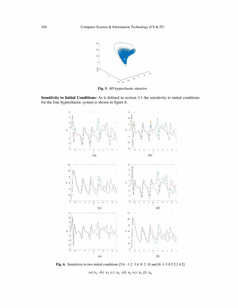
104 Computer Science & Information Technology (CS & IT)
Fig. 5. 6D hyperchaotic attractor
Sensitivity to Initial Conditions: As it defined in section 3.1 the sensitivity to initial conditions
for the four hyperchaotic system is shown in figure 6.
(a) (b)
(c) (d)
(e) (f)
Fig. 6. Sensitivity to two initial conditions [5.6 -1.2 3.4 0 2 4] and [6 -1 3 0.5 2.3 4.2]
(a):�� (b): �� (c): �� (d): �� (e): �+ (f): �,

Computer Science & Information Technology (CS & IT) 105
4. PROPOSED AUDIO ENCRYPTION SCHEME
In this section, a cryptosystem based on synchronized chaotic systems is described. The aim is to
transmit encrypted audio messages from transmitter A to remote receiver B as is depicted in Figure
7. An audio message - is to be transmitted over an insecure communication channel.
Fig. 7. Chaotic cryptosystem for audio communication [22]
To avoid any unauthorized receiver located at the mentioned channel; - is encrypted prior to
transmission to generate an encrypted message [13]:
= .(-, /) (4)
by using a chaotic system . on transmitter A. The encrypted message is sent to receiver B,
where - is recovered as -0 from the chaotic decryption 1, as:
-0 = 1( , /) (5)
If . and d have used the same key /, then at receiver end B it is possible to obtain -0 = -. A se-
cure channel is used for transmission of the keys, k. Generally, this secure communication channel
is a courier and is too slow for the transmission of m. Our chaotic cryptosystem is reliable, if it
preserves the security of m, i.e. if -0 ≠ - for even the best cryptanalytic function h, given by
-′ = ℎ( ) To achieve the proposed chaotic encryption scheme, we appeal to an hyperchaotic system for en-
cryption/decryption purposes ( and 1, respectively).
The four dimensional hyperchaotic system have a number of parameters determining their dy-
namics; such parameters and initial conditions are the coding “key”, /.
5. SIMULATION RESULTS AND SECURITY ANALYSIS
In this part, via numerical simulations, we illustrate the encrypted audio transmission. We use as
transmitter and receiver the hyperchaotic system given respectively in (1), (2) and (3) for initial
conditions��� = [−1, 1, −3, 1], ��� = [−1, 1, −3, 1, 0]and ��� = [−1,1, −3,1,0,2].
The original audio signal -(6) is 22 KHz. The mentioned audio message is to be encrypted and
transmitted to the receiver.
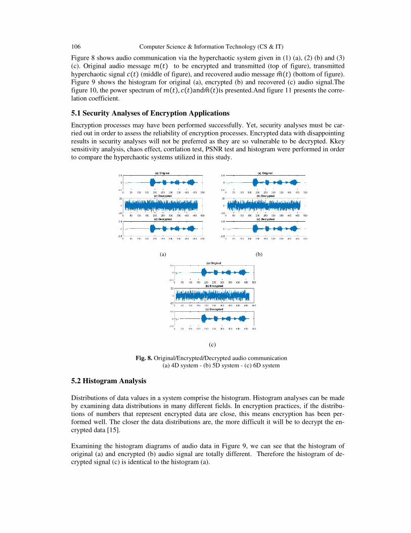
106 Computer Science & Information Technology (CS & IT)
Figure 8 shows audio communication via the hyperchaotic system given in (1) (a), (2) (b) and (3)
(c). Original audio message -(6) to be encrypted and transmitted (top of figure), transmitted
hyperchaotic signal (6) (middle of figure), and recovered audio message -0(6) (bottom of figure).
Figure 9 shows the histogram for original (a), encrypted (b) and recovered (c) audio signal.The
figure 10, the power spectrum of -(6), (6)and-0(6)is presented.And figure 11 presents the corre-
lation coefficient.
5.1 Security Analyses of Encryption Applications
Encryption processes may have been performed successfully. Yet, security analyses must be car-
ried out in order to assess the reliability of encryption processes. Encrypted data with disappointing
results in security analyses will not be preferred as they are so vulnerable to be decrypted. Kkey
sensitivity analysis, chaos effect, corrlation test, PSNR test and histogram were performed in order
to compare the hyperchaotic systems utilized in this study.
(a) (b)
(c)
Fig. 8. Original/Encrypted/Decrypted audio communication
(a) 4D system - (b) 5D system - (c) 6D system
5.2 Histogram Analysis
Distributions of data values in a system comprise the histogram. Histogram analyses can be made
by examining data distributions in many different fields. In encryption practices, if the distribu-
tions of numbers that represent encrypted data are close, this means encryption has been per-
formed well. The closer the data distributions are, the more difficult it will be to decrypt the en-
crypted data [15].
Examining the histogram diagrams of audio data in Figure 9, we can see that the histogram of
original (a) and encrypted (b) audio signal are totally different. Therefore the histogram of de-
crypted signal (c) is identical to the histogram (a).
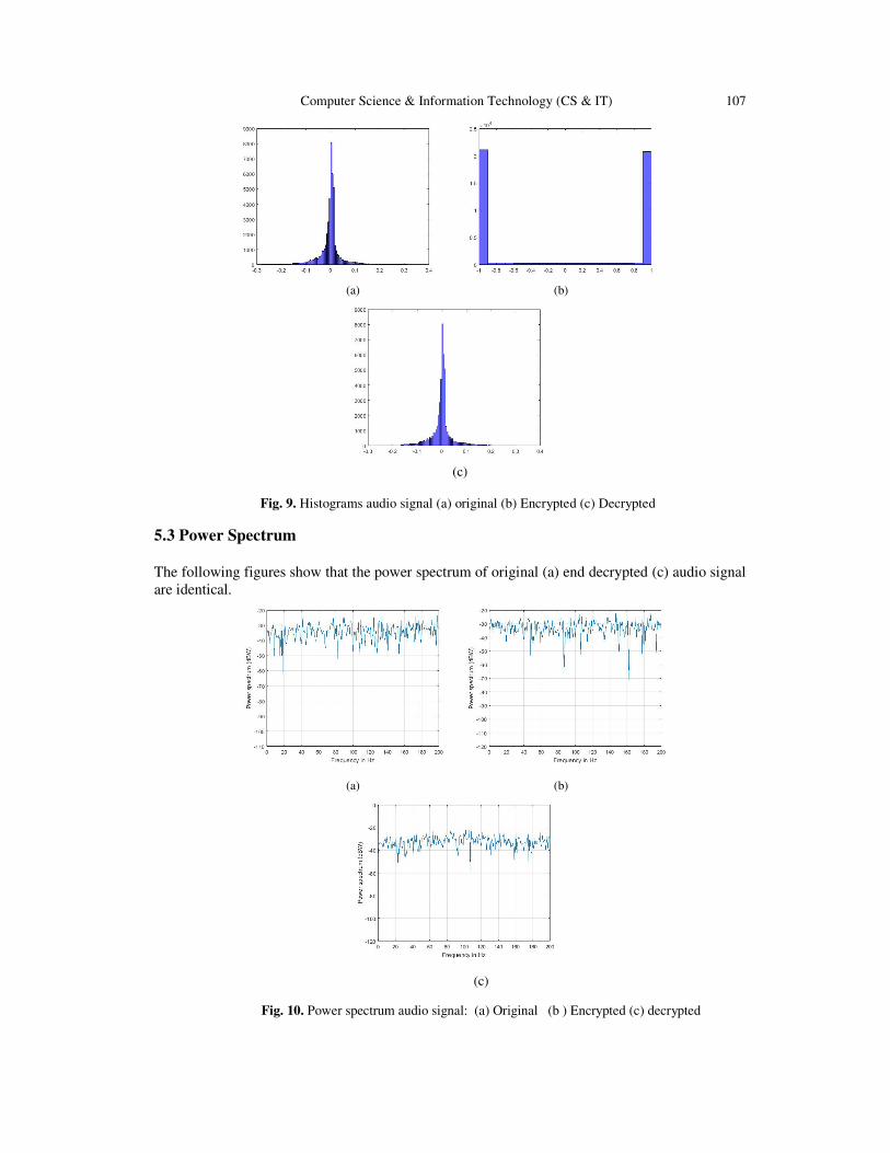
Computer Science & Information Technology (CS & IT) 107
(a) (b)
(c)
Fig. 9. Histograms audio signal (a) original (b) Encrypted (c) Decrypted
5.3 Power Spectrum
The following figures show that the power spectrum of original (a) end decrypted (c) audio signal
are identical.
(a) (b)
(c)
Fig. 10. Power spectrum audio signal: (a) Original (b ) Encrypted (c) decrypted
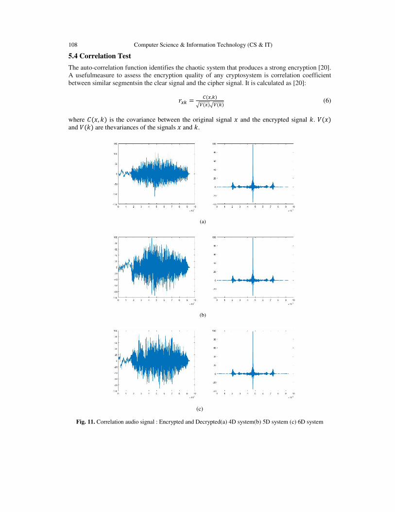
108 Computer Science & Information Technology (CS & IT)
5.4 Correlation Test
The auto-correlation function identifies the chaotic system that produces a strong encryption [20].
A usefulmeasure to assess the encryption quality of any cryptosystem is correlation coefficient
between similar segmentsin the clear signal and the cipher signal. It is calculated as [20]:
89: = ;(9,:)<=(9)<=(:) (6)
where >(�, /) is the covariance between the original signal � and the encrypted signal /. ?(�) and ?(/) are thevariances of the signals � and /.
(a)
(b)
(c)
Fig. 11. Correlation audio signal : Encrypted and Decrypted(a) 4D system(b) 5D system (c) 6D system

Computer Science & Information Technology (CS & IT) 109
5.5 PSNR test
Peak signal-to-noise ratio (PSNR) is the ratio between the maximum possible power of original
speech signal and the power of encrypted signal [20]. PSNR is a calculation of encryption quality
of the original signal. A higher PSNR indicates that the encryption or reconstruction is of higher
quality. The PSNR is obtained from:
@ABC = 10 log G9H‖9J:‖H (7)
TABLE 1 PSNR COEFFICIENT FOR AUDIO DATA
PSNR(4D) PSNR(5D) PSNR(6D)
Original/ Encrypted 47.0638 47.0558 47.0454
Original / Decrypted Inf Inf Inf
PSNR high means: Mean square error between the original and reconstructed sigal is very low. It
implies that the audio data been properly restored. In the other way, the restored signal quality is
better; in our case, the value of PSNR is as follow:
PSNR (Original/Decrypted) = Inf
Contrariwise, a low PSNR means: Mean square error between the original signal and encrypted
signal is very high. It implies that the audio data been correctly encrypted. In our case the value of
PSNR is shown is Table 1.
The result is much closed with the correlation coefficient.
- The correlation coefficients for the original and decrypted signal are identical. The value of
PSNR (Original/Decrypted) means that the decrypted audio data is identical to original data.
- The correlation coefficients for the original and encrypted signal are very different. The
PSNR(Original/Encrypted) means that the encrypted audio data is totally different of the original
data.
Speech encryption using hyperchaotic generator is a proven model. In this method, the three dif-
ferent dimensional hyperchaotic systems are applied. The histogram of the encrypted signal shows
that more sensitivity entails more security. We have found the same histogram for the original and
the decrypted audio data. The decrypted signal is very similar to the original speech as it shows the
stability of reconstruction of original signal. Correlation test and PSNR testing methods are applied
to estimate the performance of the system.
6. CONCLUSION In this article, an audio signal encryption/ decryption algorithm was designed using the three pro-
posed hyperchaotic systems. The results of the simulation showed that the encryption method of-
fered by the audio signal was highly secure and that it could quickly recover the original signal
with good audio quality. The results show that the vocal signal is highly masked by indiscreet ears.
Statistical analysis using histograms, PSNR, correlation and power spectrum showed that the algo-
rithm is powerful. From these results we will extend our studies to secure video frames as well as
real-time transmissions using the 7 dimensional hyperchaotic system.

110 Computer Science & Information Technology (CS & IT)
REFERENCES [1] Bhaskar Mondal and Tarni Mandal, “A Multilevel Security Scheme using Chaos based Encryp-tion
and Steganography for secure audio communication, Jharkhand.
[2] S. Lian, Y. Mao, and Z. Wang, "3D Extensions of Some 2D Chaotic Maps and Their Usage in Data
Encryption," in Control and Automation, 2003. ICCA '03. Proceedings. 4th International Conference
on, 2003, pp. 819-823.
[3] M. Y. Roueida , “ A Cryptographic Scheme For Color Images” , M.Sc. Thesis, Iraqi Commission For
Computers & Informatics, Informatics Institute For Postgraduate Studies 2006.
[4] C. Yun, Q. Runhe, F. Yuzhe , “Color Image Encryption Based On Hyper-Chaos“ ,Information And
Technology Department, Donghua University, Shanghai, China, pp.1-6, IEEE 2009.
[5] L. M. Pecora and T.L. Carroll, Synchronization in chaotic systems, Phys.
[6] D. López-Mancilla and C. Cruz-Hernández, Output synchronization of chaotic systems: model-
matching approach with application to secure communication, Nonlinear Dynamics and Systems
Theory, 5 (2), 141- 15 (2005).
[7] C. Cruz-Hernández and A.A. Martynyuk, Advances in chaotic dynamics with applications, Cambridge
Scientific Publishers Ltd., Vol. 4, (2009).
[8] U. Feldmann, M. Hasler and W. Schwarz, Communication by chaotic signals: the inverse sys-tem ap-
proach, Int. J. Circuits Theory and Applications, 24, 551-579 (1996).
[9] Xiaogang Wu, Hanping Hu and Baoliang Zhang, “Analyzing and improving a chaotic encryp-tion
method”, Chaos, Solitons & Fractals, Vol. 22, Issue 2, pp. 367-373, October 2004.
[10] S. N. Lagmiri, N. Elalami, J. Elalami. “Three Dimensional Chaotic System for Color Image Scram-
bling Algorithm”. International Journal of Computer Science and Information Security (IJCSIS), Vol.
16, No. 1, January 2018.
[11] M. Delgado-Restituto, M. Linan and A. Rodriguez-Vazquez, “CMOS 2.4pm chaotic oscillator: expe-
rimental verification of chaotic encryption of audio”, Electronics Letters, Vol. 32, Issue 9, pp.795-796,
1996.
[12] Wenwu Yu and Jinde Cao, “Cryptography based on delayed chaotic neural networks”, Physics Letters
A, Vol. 356, Issues 4-5, pp. 333-338, August 2006.
[13] Chang CC, Lee RTC, Xiao GX, Chen TS“A new Speech Hiding Scheme based upon sub-band cod-
ing”. Proceedings of the 2003 Joint Conference of the Fourth International Conference on Information,
Communications and Signal Processing and Fourth Pacific Rim Conference on Multimedia. Vol. 2, pp.
980– 984, (2003).
[14] L. Abraham, N. Daniel, “An improved color image encryption algorithm with Pixel permutation and
bit substitution” International Journal of Research in Engineering and Technology. Vol: 02, Issue: 11,
Nov-2013.
[15] S. N. Lagmiri1, J. Elalami, N. Sbiti, M. Amghar, " Hyperchaos for improving the security of medical
data", International Journal of Engineering & Technology, 7 (3) , June 2018 1049-1055.
[16] Chang CC, Lee RTC, Xiao GX, Chen TS (2003). A new Speech Hiding Scheme based upon sub-band
coding. Proceedings of the 2003 Joint Conference of the Fourth International Conference on Informa-
tion, Communications and Signal Processing and Fourth Pacific Rim Conference on Multimedia. Vol.
2, pp. 980– 984.

Computer Science & Information Technology (CS & IT) 111
[17] Chen S, Leung H, Ding H (2007). Telephony Speech Enhancement by Data Hiding. IEEE Transactıons
On Instrumentatıon And Measurement. Vol. 56, no. 1, pp. 63–74.
[18] Dipu KHM, Alam SB (2010). Hardware based real time, fast and highly secured speech commu-
nication using FPGA. IEEE International Conference on Information Theory and Information Security,
pp. 452–457.
[19] L. M. Pecora and T.L. Carroll, “Synchronization in chaotic systems”, Phys Rev Lett. Vol. 64, No. 8,
(1990),pp: 821-824.
[20] P. Sathiyamurthi* and S. Ramakrishnan. “Speech encryption using chaotic shift keying for secured
speech communication”. Sathiyamurthi and Ramakrishnan EURASIP Journal on Audio, Speech, and
Music Processing (2017) 2017:20.
[21] Matej Salamon (2012), “Chaotic Electronic Circuits in Cryptography”, From the book Applied Cryp-
tography and Network Security, InTech.
[22] Shujun Li, Guanrong Chen, Kwok-Wo Wong, Xuanqin Mou and Yuanlong Cai, “Baptista-type chaotic
cryptosystems: problems and countermeasures”, Physics Letters A, Vol. 332, Issue 5-6, pp 368-375,
November 2004.
[23] L.Keuninckx, M. C. Soriano, I. Fischer, C. R. Mirasso, R. M. Nguimdo & G. Van der Sande, “Encryp-
tion key distribution via chaos synchronization”, Scientific Reports volume 7, Article number: 43428
(2017).
AUTHORS
Dr. Souad Najoua LAGMIRI received the PhD degree in Computer Science, Net-
works and Security from Mohammadia School Engineering, Mohamed V University
in Rabat, Morocco. Her research interests include cryptographie of image, audio and
video.
Pr. Hassane BAKHOUS
Consultant Engineer in Information System and Computer Project Management.
Professor and Pedagogical Manager
Higher Institute of Management Administration and Computer Engineering

112 Computer Science & Information Technology (CS & IT)
INTENTIONAL BLANK

Natarajan Meghanathan et al. (Eds) : DaKM, SIPP, CCSIT, NCWMC - 2018
pp. 113–122, 2018. © CS & IT-CSCP 2018 DOI : 10.5121/csit.2018.81508
RESEARCH ON CRO'S DILEMMA IN
SAPIENS CHAIN: A GAME THEORY
METHOD
Jinyu Shi1, Zhongru Wang
1,2, Qiang Ruan
3, Yue Wu
1 and Binxing Fang
1
1Key Laboratory of Trustworthy Distributed Computing and Service (BUPT),
Ministry of Education, Beijing, China 2Zhejiang Lab, Hangzhou, China
3Beijing DigApis Technology Co., Ltd, Beijing, China
ABSTRACT
In recent years, blockchain-based techniques have been widely used in cybersecurity, owing to
the decentralization, anonymity, credibility and not be tampered properties of the blockchain.
As one of the decentralized framework, Sapiens Chain was proposed to protect cybersecurity by
scheduling the computational resources dynamically, which were owned by Computational
Resources Owners (CROs). However, when CROs in the same pool attack each other, all CROs
will earn less. In this paper, we tackle the problem of prisoner’s dilemma from the perspective
of CROs. We first define a game that a CRO infiltrates another pool and perform an attack. In
such game, the honest CRO can control the payoffs and increase its revenue. By simulating this
game, we propose to apply Zero Determinant (ZD) strategy on strategy decision, which can be
categorized into cooperation and defecting. Our experimental results demonstrate the
effectiveness of the proposed strategy decision method.
KEYWORDS
Cybersecurity, Blockchain, Game Theory, CRO's Dilemma
1. INTRODUCTION With the development of the Internet, cybersecurity becomes more and more important and
serious. In the first half of 2018, according to the report published by CNVVD [1], 10,644
vulnerabilities were discovered, which exceeded 9,690 vulnerabilities in the same period of 2017.
To protect cybersecurity, the users tend to seek professional security detection services, which are
provided by a centralized trust third part. However, this mode has the following drawback. First,
traditional security management is built in the centre environment, while attacks on the central
nodes may devastate private data. Second, the traditional methods cannot provide a trust security
platform for all participants, which can protect their privacy and avoid information leakage. Third,
the white hat hackers earn little such that they almost have no interests.
To deal with the aforementioned problems, the blockchain-based security methods have been
proposed. J.H et al. [3] study how to adapt blockchain security to cloud computing. In [4],
blockchain-based approaches which improve the security of the Internet of Things (IoT) have
been proposed. Blockchain can provide good solutions for security management and data storage
[5-10].

114 Computer Science & Information Technology (CS & IT)
Recently, a new blockchain-based security framework, Sapiens Chain, which can provide a trust
vulnerability crowd testing environment and intelligent security detection services, was proposed.
Sapiens Chain runs smart contracts on the blockchain, which guarantees the trustworthy and not
be tampered for transactions. It schedules the CROs dynamically, where CROs donate their own
computing resources and are awarded after they finish the specific tasks. In order to increase the
possibilities of rewarding, CROs tend to choose an open pool and cooperate with other CROs. In
an open pool, CROs can be categorised into honest CROs and dishonest CROs. Dishonest CROs
may reduce their consumption by forging work proofs, where they can also earn a certain amount
of income with negative absenteeism. This is unfair for honest CROs, and thus we propose to
tackle this challenge in this paper.
In this paper, we propose to use ZD (Zero-Determinant) strategies for CRO’s selection. The ZD
strategy was proposed in the Press and Dyson [15]. In the process of iterated games, one can use
the ZD strategy to control the opponent's payoff unilaterally, so that the opponent's payoff
maintains a linear relationship with hers. In other words, using ZD strategy can control the game
unilaterally. As a probabilistic and conditional strategy, the ZD strategy has been widely
employed in the iterated game, which aims to cope with the “free-riding” problems [11-13]. For
example, Eyal et al. [14] qualitatively analysed the prisoner's dilemma in the mining process,
which is a real instance of “free-riding” problems. Press et al. [15] proved that with ZD strategies,
the player is able to unilaterally set the expected utility of an opponent or a ratio of the player’s
expected payoff to its opponent’s, ignoring the opponent’s strategy. Many other studies [16-21]
on the strategy have shown the honest miners of blockchain can control opponents’ payoffs.
In summary, we make the following contributions.
First, we review the overview of Sapiens Chain, including the architecture and the roles. Then we
define the game that a CRO infiltrates another and perform an attack. In such kind of game, the
honest CRO can control the payoffs and increase its revenue.
Second, we introduce different strategies for CROs and analyze how to apply Zero Determinant
(ZD) on strategy decision, which can be categorized into cooperation or not.
Third, we report an extensive experimental study with numerical simulation. The results clearly
show that the proposed strategy decision method is effective.
The rest of this paper is organized as follows. We review the overview of Sapiens Chain in
Section 2. In Section 3, we analyze the CRO selection strategy in Sapiens Chain based on the ZD
strategy. We report the empirical evaluation results in Section 4, and conclude the paper in
Section 5.
2. THE OVERVIEW OF SAPIENS CHAIN
Sapiens Chain is a decentralized security detection platform, including the decentralized
vulnerability platform and the automatic vulnerability detection system. It contains two kinds of
nodes which are the ordinary nodes and fog nodes respectively.

Computer Science & Information Technology (CS & IT) 115
Figure 1. The architecture of Sapiens Chain
The ordinary nodes perform task publishing, POC writing, auditing and vulnerability detection,
while the fog nodes are responsible for node scheduling, vulnerability storage, POC storage,
vulnerability detection report storage, and key assignment for each ordinary node. There are 6
different roles on the ordinary nodes, which are the user, the POCD, the POCA, the WHH, the
WHA and the CRO. The user submits the requirement, which needs to be detected by Sapiens
Chain. The POCD provides POCs, which will be audited by the POCA. The WHH is the provider
that can supply manual detection services, and the WHA tests the auditing reports submitted by
WHHs.
The most important role in automatic detection is CRO, which is the computational resource
provider. CROs in Sapiens Chain are similar to miners in blockchain. It deploys automated
vulnerability detection tools and POCs, meanwhile being scheduled by the fog nodes with a pre-
defined scheduling algorithm. As a participant in each mission, the CRO contributes its own
computing power and then gains the benefit, which saves operating costs and makes Sapiens
Chain decentralized. This model of blockchain also enhances the enthusiasm of the CRO and
makes Sapiens Chain more robust.
The architecture of Sapiens Chain is shown in Figure 1. The user issues a requirement to the fog
node, and the fog node schedules CROs, WHHs or WHAs according to the given requirements.
CROs receive security plug-ins which are provided by POCDs and audited by POCAs and then
run detection processes. The vulnerabilities submitted by WHHs will be audited by WHAs and
finally received by the fog nodes, while WHHs can also submit vulnerabilities to users through
the fog nodes. The fog nodes can distribute requirements and collect reports.
3. ANALYSIS ON STRATEGY DECISION FOR CROS
In this section, we first introduce the game between honest and dishonest CROs, and then propose
the selection strategies in Sapiens Chain.

116 Computer Science & Information Technology (CS & IT)
3.1 The Game model The definitions of the honest CROs and dishonest CROs root in the Bitcoin mining problem. The
dishonest CROs are also called attacker because they may initiate Block Withholding Attacks.
That is, once the attackers have found the complete Proof-of-Work, they can choose to abandon
the proof and only send partial Proof-of-Work to the mining pool. Through this kind of attack, the
attackers will gain the payoff from the mining pool, but the mining pool can’t benefit from the
computing power of attackers. This will reduce the payoff of all CROs in this mining pool.
Sapiens Chain allows participants to use mining pools for increasing the computing power.
Unfortunately, in Sapiens Chain mining pools, dishonest CROs will earn benefit through
sabotage, such as counterfeiting Proof-of-Work. It is similar to the prisoner's dilemma which is a
classic model of game theory and was first proposed by Albert Tucker [22].
The prisoner's dilemma describes the game process of two prisoners, which is shown as follows.
The police separately interrogate two prisoners to prevent collusion. At the same time, the police
offers several options, that is, (1) if X and Y both remain silent, both of them will only
serve 3 years in prison; (2) if X betrays Y but Y remains silent, X will be set free and Y will
serve 5 years in prison; (3) if X and Y both betray the other, each of them will serves 1
year in prison.
Table 1. The payoff matrix in prisoner’s dilemma.
C D
C (R, R) (S, T)
D (T, S) (P, P)
Similar to the above situation, we introduce the prisoner’s dilemma in Sapiens Chain as follows.
Denote C, D, R, S, T and P as “Cooperation”, “Defecting”, “Reward for mutual cooperation”,
“Sucker’s payoff”, “Temptation to defect” and “Punishment for mutual defection” respectively.
Table 1 shows the prisoner’s dilemma payoff matrix in Sapiens Chain. Since T>R>P>S, the
prisoner’s dilemma game in Sapiens Chain exists. Dishonest CROs choose to attack for
increasing benefits, resulting in a decreasing of honest CROs’ payoff. Facing this prisoner's
dilemma, the CROs tend to raise their own payoff by launching attacks.
3.2 ZD strategies in Sapiens Chain
In the open pool of Sapiens Chain, the interaction between honest CROs and dishonest CROs is
regarded as an iterative game. At each iteration, we model the process as a single stage of
prisoner’s dilemma game and we suppose that long-memory player has no advantage over the
short-memory player. Thus, the actions of both CROs only depend on the rewards obtained from
the previous round.
Let 1 2 3 4( , , , )p p p p=p and 1 2 3 4( , , , )q q q q=q be the probabilities of cooperation or attacking
based on the previous iteration for the honest CRO X and the dishonest CRO Y. We use a
parameter (0 1)m m< < to represent the reduced ratio of the cooperation rate for CROs who
betrayed last time. Thus we can rewrite p and q as1 2 3 4( , , , )p p pm mp=p and
1 2 3 4( , , , )q mq q mq=q respectively, which represent the transition probability vectors for the
cooperation state in the next round. Then we mode an iterated game as a Markov process, and we
can build the Markov matrix as shown in Equation (1).

Computer Science & Information Technology (CS & IT) 117
( ) ( ) ( )( )( ) ( ) ( )( )
( ) ( ) ( )( )( ) ( ) ( )( )
1 1 1 1 1 1 1 1
2 3 2 3 2 3 2 3
3 2 3 2 3 2 3 2
4 4 4 4 4 4 4 4
1 1 1 1
1 1 1 1
1 1 1 1
1 1 1 1
p q p q p q p q
p mq p mq p mq p mq
mp q mp q mp q mp q
mp mq mp mq mp mq mp mq
− − − −
− − − − = − − − −
− − − −
P (1)
Since matrix P has a unit eigenvalue, the matrix = −M P I (see Equation (2)) must be a
singular matrix and 0=M . M can be expressed as:
( ) ( ) ( )( )( ) ( ) ( )( )( ) ( ) ( )( )( ) ( ) ( )( )
1 1 1 1 1 1 1 1
2 3 2 3 2 3 2 3
3 2 3 2 3 2 3 2
4 4 4 4 4 4 4 4
1 1 1 1 1
1 1 1 1 1
1 1 1 1 1
1 1 1 1 1
p q p q p q p q
p q p q p q p q
mp mq mp mq mp mq mp mq
mp mq mp mq mp mq mp mq
− − − =
− −
− − − − −
− − − − −
− − − − −
M (2)
Let 0= =,
T T Tv P v v M . Then we can obtain the stationary vector [ ]1 2 3 4, , ,T
v v v v=v of
M . Given *M as shown in Equation (3), according to the Cramer’s ruler, we have
( )det 0= =I*M M M , where ( ) ( )1 deti j
ijc+
= − '
ijM and [ ]1 2 3 4, , ,v v v v is proportional to
[ ]14 24 34 44, , ,c c c c . It follows,
[ ] ( )
1
2
1 2 3 4
3
4
1 1 1 1 1
2 3 2 3 2
3 2 3 2 3
4 4 4 4 4
1 1 1
1
1
f
fv v v v D p q
f
f
p q p q f
p mq p mq fdet
mp q mp q f
mp mq mp mq f
= ≡
− + − + − + − + = − +
, , , , ,
Tv f f
(3)
Let α β γ= + +X Yf S S 1 . The expected payoff of CRO X and CRO Y in the stationary state
satisfies Equation 4, where , ,α β γ are non-zero parameters.
( )
( )α β γ
+ ++ + =
, , X
X
Y
Y
D p q αS βS γ1S S 1
D p, q, 1 (4)
Let ( ) ( )1 2 3 41, 1 ,, φT
p p mp mp α β γ= − − = + +X Yp S S 1 . It follows

118 Computer Science & Information Technology (CS & IT)
( )1
2
3
4
r c1 φ
2
r r1 φ
2 2
r rφ
2 2
φ
p
p c
c
pm
pm
α β γ
α β γ
β α γ
γ
− = + + +
= + − + +
− + +
=
=
(5)
From the above analysis, we can know that if the CRO X takes strategies of α XS , β YS or a
linear combination of them, it will have the possibility to choose unilateral strategies and make
the determinant in numerator in Equation (4) vanish. Similarly, the same to CRO Y. Thus if the
CRO X adopts a strategy which satisfies = α β γ+ +X Yp S S 1 , or if the CRO Y takes a strategy
with = α β γ+ +X Yq S S 1 , then the determinant vanishes. Accordingly, the payoffs of CRO X
and CRO Y will be satisfied with a linear relationship
α β γ+ + =X YS 1S 0 .
3.3 The ZD-set strategy in Sapiens Chain
In Sapiens Chain, the ZD-set strategy means that honest CRO X uses the ZD strategy to
unilaterally set the long-term benefits of dishonest CRO Y. When honest CRO X uses the ZD-set
strategy, we fix 0α = in α β γ+ + =X YS 1S 0 . Let β γ= +%Yp S 1 . We can use 1p and 4p to
represent 32 ,p p and YS , which are shown in Equation (6)-(8).
( )1 4
2
1rp c pp
r c
− +=
− (6)
( )( )1 4
3
2 1c r p cpp
r c
− − +=
− (7)
( )
( )4
1 42 1
p r c
p p
−=
− +YS (8)
Thus, we can conclude that, when CRO X takes a ZD-set strategy, it can unilaterally set the
payoff of CRO Y, regardless of the CRO Y’s strategy, while the CRO X can’t control its own
payoff even with any subclass of ZD strategy.
3.4 The ZD-extortion strategy in Sapiens Chain In Sapiens Chain, the ZD-extortion strategy means that honest CRO X uses the ZD strategy to
unilaterally set the long-term return of dishonest CRO Y to be linear with his own earnings. If
honest CRO X uses the ZD-extortion strategy, it can also guarantee that the other party's payoff is
always lower than its own payoff. Since ZD-extortion strategy always passes the reference

Computer Science & Information Technology (CS & IT) 119
point l P= , we have ( ) ( )( )φ s P P= − − −%X Yp S S , where 1s < . 31 2 4, , ,p p p p can be
represented as follows, which are shown in Equation (9).
( )1
2
3
4
r c1 φ 1 s
2
r r1 φ s
2 2
r rφ s
2 2
0
p
p c
p c
p
−= − − ⋅
= − − +
= − + ⋅
=
(9)
If ϕ is small enough, there exists a viable extortion strategy for any s . Since 31 2 4, , ,p p p p are
all between[0,1] . It follows,
( )r c
0 1 φ 1 s 12
r r0 1 φ s 1
2 2
r r0 φ s 1
2 2
c
c
−≤ − − ⋅ ≤
≤ − − + ≤
≤ − + ⋅ ≤
(10)
The range of ϕ can be represented in Equation (11).
1
0 φr r
s2 2
c
≤ ≤
− +
(11)
Since ϕ is small enough, the range of extortion factor s can satisfy 2
s 1r c
r
−≤ < . Following
ZD-extortion strategy, CRO X will have a larger payoff than CRO Y.
4. EXPERIMENTS In this section, we use numerical simulation to illustrate the performance of the different
strategies in the prisoner's dilemma. We use WSLS, ALLD and ALLC as the comparison
strategies, where WSLS strategy is “win stay, lose shift”, ALLD strategy is “Always Defecting”
and ALLC strategy is “Always Cooperation”. Fix 1.5R = , 1S = − , 3T = , 0P = then the
payoff vector of the honest CRO X will be ( )1.5, 1,3,0= −XS , and that of the dishonest CRO Y
will be ( )1.5,3, 1,0= −YS . For each experiment, we evaluate the differences of the payoffs
between the honest CRO X and the dishonest CRO Y. All figures show the possible payoffs of
the CRO X (on the horizontal axis) and the CRO Y (on the vertical axis) as colored areas or lines,
where the colored points represent the payoff pairs for 50, 000 chosen opponents.
In Figure 2, when honest CRO X adopts the WSLS strategy and dishonest CRO Y takes a
strategy randomly, the payoff of the two CROs shows that the profit coverage area is a triangle.

120 Computer Science & Information Technology (CS & IT)
Figure 2. The payoff of two CROs (WSLS VS Random)
In Figure 3, when honest CRO X always adopts a cooperative or betrayal strategy, and dishonest
CRO Y takes a strategy randomly, the payoffs of the two CROs shows that the profit coverage
area is a straight line.
Figure 3. The payoff of two CROs (ALLC, ALLD VS Random)
In Figure 4, when honest CRO X adopts the ZD-set strategy and dishonest CRO Y also takes a
strategy randomly, the profit of the two CROs shows that the honest CRO X can dominate the
opponent's benefit which is always on a straight line.
Figure 4. The payoff of two CROs (ZD-set VS Random)

Computer Science & Information Technology (CS & IT) 121
In Figure 5, when honest CRO X adopts the ZD-extortion strategy and dishonest CRO Y takes a
strategy randomly, the payoffs of the two CROs shows that the CRO X can control not only the
opponent's income which is always on a straight line, but also his benefit higher than s times the
other’s.
Figure 5. The payoff of two CROs (ZD-extortion VS Random)
Compared with ZD strategy, the WSLS, ALLC, and ALLD strategies have no restrictions on the
payoffs. When it comes to the ZD-set strategy, it can achieve the goal that honest CRO X restricts
dishonest CRO Y, and the ZD-extortion strategy can guarantee that the profit of honest CRO X is
higher than dishonest CRO Y’s. We attempt to apply ZD strategy to Sapiens Chain. No matter
what strategy the dishonest CROs adopt, when honest CROs adopt the ZD strategy, the payoff of
dishonest CROs can be restricted. What’s more, honest CROs can keep the payoffs of dishonest
CROs linear with their own earnings, which makes it possible to design efficient game consensus.
5. CONCLUSION In this paper, we first define a game that a CRO infiltrates another and perform an attack. In such
game, the honest CRO can control the payoff and increase its revenue. By simulating this game,
we propose to apply Zero Determinant (ZD) on strategy decision, which can be categorized into
cooperation or not. Our experimental results demonstrate the effectiveness of the proposed
strategy decision method, indicating that the honest CROs can apply ZD strategy to control the
payoffs of themselves higher than dishonest CROs. Due to ZD strategy, CROs become more
energetic and Sapiens Chain becomes safer.
REFERENCES [1] Ehrenfeld, J. M. (2017). Wannacry, cybersecurity and health information technology: A time to act.
Journal of medical systems, 41(7), 104.
[2] Nakamoto, S. (2008). Bitcoin: A peer-to-peer electronic cash system.
[3] Park, J. H., & Park, J. H. (2017). Blockchain security in cloud computing: Use cases, challenges, and
solutions. Symmetry, 9(8), 164.
[4] Dorri, A., Kanhere, S. S., Jurdak, R., & Gauravaram, P. Blockchain for IoT Security and Privacy: The
Case Study of a Smart Home.
[5] Yuan, Y., & Wang, F. Y. (2016). Blockchain: the state of the art and future trends. Acta Automatica
Sinica, 42(4), 481-494.

122 Computer Science & Information Technology (CS & IT)
[6] Eyal, I., & Sirer, E. (2014). It’s time for a hard Bitcoin fork. Hacking, Distributed, 13.
[7] Rosenfeld, M. (2011). Analysis of bitcoin pooled mining reward systems. arXiv preprint
arXiv:1112.4980.
[8] Courtois, N. T., & Bahack, L. (2014). On subversive miner strategies and block withholding attack in
bitcoin digital currency. arXiv preprint arXiv:1402.1718.
[9] McWaters, R., Bruno, G., Galaski, R., & Chaterjee, S. (2016). The future of financial infrastructure:
An ambitious look at how blockchain can reshape financial services. In World Economic Forum.
[10] Melanie, S. (2015). Blockchain: blueprint for a new economy. Sebastopol: O'Reilly Media.
[11] Nowak, M., & Sigmund, K. (1993). A strategy of win-stay, lose-shift that outperforms tit-for-tat in the
Prisoner's Dilemma game. Nature, 364(6432), 56.
[12] Rapoport, A., Chammah, A. M., & Orwant, C. J. (1965). Prisoner's dilemma: A study in conflict and
cooperation (Vol. 165). University of Michigan press.
[13] Axelrod, R. (1987). The evolution of strategies in the iterated prisoner’s dilemma. The dynamics of
norms, 1-16.
[14] Eyal, I. (2015, May). The miner's dilemma. In Security and Privacy (SP), 2015 IEEE Symposium on
(pp. 89-103). IEEE.
[15] Press, W. H., & Dyson, F. J. (2012). Iterated Prisoner’s Dilemma contains strategies that dominate
any evolutionary opponent. Proceedings of the National Academy of Sciences, 109(26), 10409-
10413.
[16] Pan, L., Hao, D., Rong, Z., & Zhou, T. (2015). Zero-determinant strategies in iterated public goods
game. Scientific reports, 5, 13096.
[17] Dong, H., Zhi-Hai, R., & Tao, Z. (2014). Zero-determinant strategy: An underway revolution in game
theory. Chinese Physics B, 23(7), 078905.
[18] Adami, C., & Hintze, A. (2013). Evolutionary instability of zero-determinant strategies demonstrates
that winning is not everything. Nature communications, 4, 2193.
[19] Hilbe, C., Wu, B., Traulsen, A., & Nowak, M. A. (2015). Evolutionary performance of zero-
determinant strategies in multiplayer games. Journal of theoretical biology, 374, 115-124.
[20] Al Daoud, A., Kesidis, G., & Liebeherr, J. (2014). Zero-determinant strategies: A game-theoretic
approach for sharing licensed spectrum bands. IEEE Journal on Selected Areas in Communications,
32(11), 2297-2308.
[21] Chen, J., & Zinger, A. (2014). The robustness of zero-determinant strategies in iterated prisoner׳ s
dilemma games. Journal of theoretical biology, 357, 46-54.
[22] Burgum, E. B. (1950). The novel and the world's dilemma.

Natarajan Meghanathan et al. (Eds) : DaKM, SIPP, CCSIT, NCWMC - 2018
pp. 123–133, 2018. © CS & IT-CSCP 2018 DOI : 10.5121/csit.2018.81509
SAPIENS CHAIN: A BLOCKCHAIN-BASED
CYBERSECURITY FRAMEWORK
Yu Han1, Zhongru Wang
1,2, Qiang Ruan
3 and Binxing Fang
1
1Key Laboratory of Trustworthy Distributed Computing and Service (BUPT),
Ministry of Education, Beijing, China 2Zhejiang Lab, Hangzhou, China
3Beijing DigApis Technology Co., Ltd, Beijing, China
ABSTRACT
Recently, cybersecurity becomes more and more important due to the rapid development of
Internet. However, existing methods are in reality highly sensitive to attacks and are far more
vulnerable than expected, as they are lack of trustable measures. In this paper, to address the
aforementioned problems, we propose a blockchain-based cybersecurity framework, termed as
Sapiens Chain, which can protect the privacy of the anonymous users and ensure that the
transactions are immutable by providing decentralized and trustable services. Integrating
semantic analysis, symbolic execution, and routing learning methods into intelligent auditing,
this framework can achieve good accuracy for detecting hidden vulnerabilities. In addition, a
revenue incentive mechanism, which aims to donate participants, is built. The practical results
demonstrate the effectiveness of the proposed framework.
KEYWORDS
Cybersecurity, Blockchain, Decentralized Model
1. INTRODUCTION In recent years, the applications of Internet of Things, Internet of Vehicles, and Mobile Payment
have been more and more popular and deeply affect human life [1][2]. However, these
applications face more serious security risks than before [3]. For example, more than 70 countries
and regions were attacked by the newly produced computer virus WannaCrypt0r 2.0 and suffered
high damages [4]. Uber lost large scales of sensitive information, which may be related to 57
million users and 7 million drivers [5]. Besides the traditional security problems, new techniques,
such as blockchain, may become exposed to security threats. For example, the famous incident
DAO occurred in Ethereum and the attackers stole about 3.5 million Ether, which was worth
about 60 million dollars at that time, owing to a smart contract vulnerability [5] [6]. The high
yield of successful attacks drives the “prosperity” of the black industry.
To deal with the aforementioned cybersecurity problems, many studies are proposed [7-10]. Not
surprisingly, existing methods mostly focus on centralized models and have the following
drawbacks. First, it’s difficult to manage data storage and security dynamically. Traditional data
storage and security management are always built in the trust and centralized environment, while
attacks on the central management nodes may devastate private data and the networks [11].
Second, it’s hard to cope with the high-intensity attacks timely with limited resources. In addition,
the participants require a security interactive platform, which can protect their privacy and avoid

124 Computer Science & Information Technology (CS & IT)
information leakage. Third, the white hat hackers can only obtain little revenue from the security
vendors, such that they have low interests in helping vendors fix their vulnerabilities.
To tackle these challenges, we design a blockchain-based framework, named by Sapiens Chain,
that protects all participants by using a decentralized, non-monopoly and non-intermediate model.
We make the following contributions in this work.
First, we design a smart contract for all participants, where the transactions are written into blocks
and almost impossible to be modified. By defining the incentive mechanism on smart contracts,
the Proof-Of-Cnocept (POC) providers can be awarded if the task result is adopted by the
framework. The task details and identities of participants will be disclosed, such that the privacy
of participants is guaranteed.
Second, we introduce two kinds of nodes, including the ordinary nodes and the fog nodes.
Ordinary nodes perform task assignment, vulnerability detection, POC construction, and POC
auditing, while the fog nodes perform node scheduling and storage for POCs and vulnerabilities.
For reducing the computational resource overhead as much as possible, we propose a novel node
scheduling method, which combines the proof of work with the distances between nodes.
Third, we propose a novel model that can audit websites, applications and smart contracts auto-
matically. For websites, the model can automatically identify network assets and vulnerabilities
through knowledge graphs and association rules. For applications and smart contracts, the model
first extracts basic semantic information through dependency graphs, and then discover vulner-
abilities within the codes by performing analysis on the semantic information.
The rest of the paper is organized as follows. We review the related work in Section 2 and
propose the framework in Section 3. Section 4 introduces roles, techniques and operational modes
of the framework. We introduce the typical application in Section 5 and conclude the paper in
Section 6.
2. RELATED WORK In this section, we review some related work, including the existing blockchain-based
cybersecurity protection methods and systems.
2.1. Blockchain-based Cybersecurity Studies Many novel cybersecurity techniques have been used in website security [12] [13], application
security [14] and blockchain security [15]. For example, Nikolic et al. [16] present MAIAN, the
first tool for precisely specifying and reasoning about trace properties, which employs inter-
procedural symbolic analysis and concrete validator for exhibiting exploits. Tsankoc et al. [8]
present Securify, a security analyzer for Ethereum smart contracts that is scalable, and able to
prove contract behaviors as safe/unsafe with respect to a given property.
Recently, blockchain technology has made significant contributions to cybersecurity due to its
immutability, traceability, decentralization, and transparency [12-17]. Zyskind et al. [18] propose
to protect application data using blockchain, which separates data from permissions, records
permission settings and data access in blockchain, enabling full control of data access permissions
and transparent access procedures. Azaria et al. [19] propose a medical data management model
based on blockchain and smart contract, which records data permissions and operations in the
blockchain, and is executed by smart contracts to implement data authentication, confidentiality,
auditing, and sharing. Buldas et al. [20] propose a blockchain-based keyless signature framework,

Computer Science & Information Technology (CS & IT) 125
which records the root hash value in the chain and performs multi-file signature, which increases
the overhead of falsifying signature files, ensuring the integrity of the file. Ali et al. [21] propose
a distributed domain name resolution system based on blockchain, where this system can
effectively resist DDoS attacks by layering the domain name resolution logic and the underlying
consensus mechanism.
However, previous approaches focus on only one or two aspects of cybersecurity, which cannot
provide a fair and trust environment. Our framework can not only detect vulnerabilities, but also
protects all participants’ privacy by using a decentralized, non-monopoly and non-intermediate
model.
2.2. Blockchain-based Cybersecurity Applications Several applications, such as CertiK [22], SECC [23] and DVP [24], have been produced to
protect cybersecurity. CertiK uses formal verification techniques to transform smart contracts into
mathematical models and validate models through logical calculus to prove the security. The
automated auditing tools are deployed on the server and improve capabilities via plug-in provided
by white hats. In order to solve the inherent vulnerabilities of the original public chain, wallet,
and transactions, SECC essentially recreates a public chain, the nodes on which are safe nodes
and the applications on which are safe applications. DVP built a vulnerability platform on
blockchain to ensure its security. The system operates on the blockchain and provides the
required power based on the distributed network of participants, who use the agreement points to
pay, receive or enhance the verification service.
In contrast to the previous framework, Sapiens Chain can detect the vulnerabilities automatically
and can handle website security, application security, and blockchain security simultaneously.
3. THE ARCHITECTURE OF THE FRAMEWORK In this section, we first propose the overview of the proposed framework and then introduce the
structure.
The overview of the proposed framework is shown in Figure 1. The computing nodes of the
Sapiens Chain are decentralized and thus each node won’t be affected by others. The users submit
their tasks including website tasks, application tasks, and smart contract tasks through the browser,
the fog nodes in Sapiens Chain first distinguish the type of the task, and then segment tasks into
several parts, running the algorithms to select proper nodes to deal with the task, and finally
gather the results into a report.
Figure 1. Sapiens Chain overview

126 Computer Science & Information Technology (CS & IT)
The hierarchical structure of Sapiens Chain is shown as Figure 2. Sapiens Chain has 4 layers,
including the resource layer, the transport layer, the contract layer, and the application layer.
Figure 2. The architecture of Sapiens Chain layers
a) The resource layer integrates a large number of resources, which ensures that Sapiens Chain
can have a large detection capacity. The essence of the resource layer is a distributed ledger that
records the service information of all participants [25]. The record format is related to the public
chain where the framework runs, and the records are guaranteed to protect the rights of the
service provider from being infringed.
b) The transport layer, which relies on P2P network, is used to transmit information, which
includes resource scheduling and information dissemination [26]. The nodes in Sapiens Chain are
theoretically accessible to each other. The ledgers of nodes will be synchronized after finishing
tasks.
c) The contract layer is designed to contract the service process, including both consensus and
incentive and punishment mechanisms. The consensus mechanism is consistent with the
consensus mechanism of the underlying blockchain, and all kinds of nodes are ranked according
to the active level and task completion degree [27]. According to the accuracy and fairness of the
results of the consensus mechanism, this framework can achieve good audit performance. Based
on the ruling result of the consensus mechanism, the incentive and punishment mechanism
rewards or punishes nodes and writes the results of arbitration on the chain and then can protect
the rights of the contributors.
d) The application layer realizes the fragmentation and classification of tasks, and the centralized
security service of traditional security vendors is distracted, distributed to each node, therefore the
benefits are shared [28]. Each node accesses the service through the blockchain browser at the

Computer Science & Information Technology (CS & IT) 127
application layer. The distribution of the fragmentation task adopts a redundancy mechanism. The
selected nodes get several non-repeating segments, and each segment is dispersed to several non-
repeating nodes. The nodes perform three different types of tasks, which includes manual
vulnerability detecting, POC writing and auditing, and running automatic auditing tools.
4. THE OPERATION MODE OF THE FRAMEWORK
In this section, we first introduce two kinds of nodes and the inherent techniques, and then
propose how to operate this framework.
4.1. Nodes
Sapiens Chain includes two kinds of nodes: ordinary nodes and fog nodes.
4.1.1. Ordinary Nodes
The ordinary node contains 6 different roles, which is shown as follows.
• User. The user submits the tasks, which requires to be detected by Sapiens Chain. The privacy
of users and the immutability of the transactions can be protected by smart contracts defined
between users and Sapiens Chain.
• Proof of Concept Developer (POCD). The POCD provides POCs. Essentially, each node of
Sapiens Chain can be a POCD, whose gains are related to the number of accepted POCs and
called POCs.
• Proof of Concept Auditor (POCA). The POCA audits the POCs, which is provided by POCD.
The POCAs are generated through an arbitration mechanism among POCDs.
• White Hat Hacker (WHH). The WHH is the provider that can supply manual audit services.
WHHs are selected through a scheduling scheme, which is designed by Sapiens Chain.
• White Hat Auditor (WHA). The WHA is one of the WHHs, which has a higher active degree
and generated by an arbitration mechanism. Its task is to test the auditing results submitted by
WHHs.
• Computational Resources Owner (CRO). The CRO deploys an automatic vulnerability audit
tool and is called by a scheduling algorithm. As providing automatic auditing, CROs benefit from
their own computational resources, which can reduce the operating costs and increase the
enthusiasm simultaneously.
4.1.2. Fog Nodes
The fog node is responsible for node scheduling, POC storage, report storage, and key assignment
for each ordinary node [29]. It runs a proof of work and node distance-based scheduling
mechanism that can select appropriate CROs to perform the detection service. In addition, the fog
nodes can store the submitted vulnerabilities, accepted POCs and test reports, such that these
relevant resources can be reused.
Figure 3 shows how different roles of nodes interact with each other. The user issues a task to the
fog node, and the fog node schedules CROs, WHHs or WHAs according to the given tasks. CROs

128 Computer Science & Information Technology (CS & IT)
receive POCs which are provided by POCDs and audited by POCAs and then run detection
processes. The vulnerabilities submitted by WHHs will be audited by WHAs and finally received
by the fog nodes, while WHHs can also submit vulnerabilities to users through the fog nodes. The
fog nodes can distribute tasks and collect reports.
Figure 3. Roles in Sapiens Chain
4.2. The Algorithms The algorithms of Sapiens Chain can be categorized into scheduling algorithms and security
algorithms.
The scheduling algorithms called by the fog nodes, are used to allocate tasks or computational
resources dynamically according to the different roles of ordinary nodes. These algorithms run for
POCD, POCA, CRO, WHH, and WHA selection. Following the principle of proximity, the
algorithms rank the computational resources according to the proof of work mechanism and select
the nodes closest to the users [30]. Since task auditing by WHHs requires professional knowledge,
we ensure the ability of the nodes by applying the incentive mechanism and punishment
mechanism which will be introduced later.
The security algorithms use symbolic execution, taint analysis, and formal verification to detect
website, application and smart contract vulnerabilities. For websites, Sapiens Chain can detect
vulnerabilities with thousands of built-in predefined knowledge graphs and association rules,
which can automatically identify asset information and then realize deep detection of security
vulnerability. For applications and smart contracts, Sapiens Chain builds the dependency graphs
to extract basic semantic information. With these semantics and the control flow graphs, it can
match vulnerability patterns, which can avoid possible path execution errors and improve the
detection accuracy.

Computer Science & Information Technology (CS & IT) 129
4.3. Work Mode
4.3.1. Reward Mode
The reward mode refers to that the users submit tasks and then select the automatic audit service
or the manual audit service. For the automatic audit service, the CROs are scheduled by the fog
nodes to call the automatic detection tools. POCs stored in fog nodes will be installed on the tools
on CRO, and then CRO runs the tools to output a report about vulnerabilities and patches. For the
manual audit mode, the fog nodes schedule WHHs, who can also submit reports to WHAs. This
process ends until the reports are approved.
4.3.2. Claim Mode
The claim mode refers to the mode where the WHHs actively submit the vulnerabilities, which
can be claimed by users if needed. The WHHs can encrypt the details of vulnerabilities with
users’ public keys and send them to the fog nodes for storage. Then the fog nodes transport the
information to users and determine whether they will claim. The WHHs can benefit if the
vulnerabilities are claimed.
4.4. Incentive and Punishment Mechanism
4.4.1. Incentive Mechanism
In order to avoid issues of network abuse and encourage more nodes to provide computational
resources, we propose the fuel called SACF, which can be exchanged in Sapiens Chain. The
SACF can be regarded as a reward after each role provides effective services, and it can be paid
for services purchasing by users. Different roles can be rewarded under the following situations.
(1) POCDs submit POCs and the POCs are adopted after review; (2) POCAs participates in POC
audit and their final audit results are adopted, (3) WHHs submit vulnerabilities which are also
adopted, (4) WHAs audit the vulnerabilities and the results are adopted, (5) CROs provide
complete audit services and finally output an available audit report.
4.4.2. Punishment Mechanism
In order to deal with the problem of node dishonesty, we propose a punishment mechanism. For
CRO, we define a parameter that measures the average processing capacity, which corresponds to
the number of running tasks and computational resources. The parameter will drop when the CRO
did not complete the task. When this parameter of the nodes becomes zero, we will abandon such
nodes. For WHHs, if the vulnerabilities submitted in the reward mode are not approved or these
submitted in the claim mode are not successfully claimed, we will punish them and decrease their
rankings which denote the priority to be scheduled. We omit the mechanisms for POCAs and
WHAs as it’s similar to the WHH case.
5. PRACTICAL RESULTS AND TYPICAL APPLICATIONS In this section, we first introduce the practical results of the proposed framework and then
propose typical applications.
5.1. Practical Results
We implement our framework as a security auditing platform, which aims to detect risks and
vulnerabilities and give suggestions for improvement. In our framework, each selected CRO node

130 Computer Science & Information Technology (CS & IT)
is an automatic audit tool, which can audit websites, applications and smart contracts. Taking
several test websites for example, we run the CRO node and get the result as below.
As shown in Figure 4, 80% of detected websites are at low risk level, while 20% are at high level.
This demonstrates that, our framework can distinguish risk levels. As shown in Figure 5, in one
test website, we can detect 368 vulnerabilities, and 179 vulnerabilities are at high risk level. This
demonstrates that our framework is effective in detecting vulnerabilities. After detection, the node
will output a report containing specific vulnerabilities and corresponding suggestions.
Figure 4.The risk types of website
Figure 5. The risk types of vulnerabilities
5.2. Typical Applications The framework has the following application scenarios.
(1) Website, application and smart contract security. In order to protect the website from attacks,
security vendors often exploit and repair vulnerabilities with the help of the security team or the
vulnerability platform. However, the security teams of different vendors are not strong enough to
cope with the surge in cybersecurity, such that they may not identify hidden vulnerabilities.
Sapiens Chain builds a trust security audit platform for all practitioners in the field of

Computer Science & Information Technology (CS & IT) 131
cybersecurity so that we can provide vulnerability audit services with high accuracy. During the
auditing process, Sapiens Chain can protect the privacy and reward according to the donation,
which can attract more and more white hats.
(2) Shared Economy. In Sapiens Chain, CROs can earn revenue by sharing idle network
bandwidth, storage space, and computational resources. Through the trusted interactive network
built by blockchain technology, Sapiens Chain allocates resources through the scheduling
algorithms, which can closely meet the requirement of the sharing economy.
6. CONCLUSIONS In this paper, we proposed Sapiens Chain, a blockchain-based cybersecurity framework for
security detection and protection. Sapiens Chain leverages the combination of blockchain
technology and artificial intelligence that distribute computational resources and accomplish tasks
automatically. Based on blockchain, the framework collect resources for the missions, at the same
time using the distributed ledger to guarantee the immutability of the reward process. Using
artificial intelligence, each CRO node is an automated audit tool, and its audit capacities can be
continuously improved through machine learning whose samples come from the manual detection
process, which means the samples are endless. The practical results demonstrate the effectiveness
of the proposed framework.
REFERENCES [1] A. Dorri, S. S. Kanhere, R. Jurdak, and P. Gauravaram, (2017) “Blockchain foriot security and
privacy: The case study of a smart home”, in Pervasive Computing and Communications Workshops
(PerCom Workshops), 2017 IEEE International Conference on. IEEE, pp618–623.
[2] Z. Zeng and Y. Yang, (2000) “Development and research of cybersecurity”, Computer Engineering
and Applications, vol. 36, no. 10, pp1–3.
[3] A. Goranovi´ c, M. Meisel, L. Fotiadis, S. Wilker, A. Treytl, and T. Sauter, (2017)“Blockchain
applications in microgrids an overview of current projects and concepts”, in Industrial Electronics
Society, IECON 2017-43rd Annual Conference of the IEEE. IEEE, pp6153–6158.
[4] F. Sebastiani, (2002) “Machine learning in automated text categorization”, ACM computing surveys
(CSUR), vol. 34, no. 1, pp1–47.
[5] G. Wood, (2014) “Ethereum: A secure decentralised generalised transaction ledger”, Ethereum
project yellow paper, vol. 151, pp1–32.
[6] N. Atzei, M. Bartoletti, and T. Cimoli, (2017) “A survey of attacks on ethereum smart contracts
(sok)”, in Principles of Security and Trust. Springer, pp164–186.
[7] M. Zhao, L. Zhang, and J. Yu, (2017) “Blockchain-based social iot trusted service management
framework”, Telecommunications Science, vol. 33, no. 10, pp19–25.
[8] P. Tsankov, A. Dan, D. D. Cohen, A. Gervais, F. Buenzli, and M. Vechev, (2018) “Securify: Practical
security analysis of smart contracts”, arXiv preprint arXiv: 1806.01143.
[9] Y. Chen, D. Xu, and L. Xiao, (2018) “Overview of network security technology based on
blockchain”, Telecommunications Science, vol. 34, no. 3, pp10–16.
[10] Y. Yang and X. Niu, (2017) “General theory of security (14) - macro behaviour analysis of viral
malicious code”, Journal of Chengdu University of Information Technology, vol. 32, no. 1, pp8–13.

132 Computer Science & Information Technology (CS & IT)
[11] Yan, Q., Yu, F. R., Gong, Q., & Li, J, (2016) “Software-defined networking (SDN) and distributed
denial of service (DDoS) attacks in cloud computing environments: A survey, some research issues,
and challenges”, IEEE Communications Surveys & Tutorials, 18(1), 602-622.
[12] A. Akkiraju, D. Gabay, H. B. Yesilyurt, H. Aksu, and S. Uluagac, (2017) “Cybergrenade: Automated
exploitation of local network machines via single board computers”, in Mobile Ad Hoc and Sensor
Systems (MASS), 2017 IEEE 14th International Conference on. IEEE, pp580–584.
[13] R. Kachhwaha and R. Purohit, (2019) “Relating vulnerability and security service points for web
application through penetration testing”, in Progress in Advanced Computing and Intelligent
Engineering. Springer, pp41–51.
[14] Y. K. Lee, P. Yoodee, A. Shahbazian, D. Nam, and N. Medvidovic, (2017) “Sealant: A detection and
visualization tool for inter-app security vulnerabilities in androic”, in Automated Software
Engineering (ASE), 2017 32nd IEEE/ACM International Conference on. IEEE, pp883–888.
[15] A. Kosba, A. Miller, E. Shi, Z. Wen, and C. Papamanthou, (2016) “Hawk: The blockchain model of
cryptography and privacy-preserving smart contracts”, in 2016 IEEE symposium on security and
privacy (SP). IEEE, pp839–858.
[16] I. Nikolic, A. Kolluri, I. Sergey, P. Saxena, and A. Hobor, (2018) “Finding the greedy, prodigal, and
suicidal contracts at scale”, arXiv preprint arXiv: 1802.06038.
[17] Q. Shao, C. Jin, Z. Zhang, W. Qian, A. Zhou et al., (2018) “Blockchain technology: Architecture and
progress”, Journal of Computer, vol. 41, no. 5, pp969–988.
[18] G. Zyskind, O. Nathan et al., (2015) “Decentralizing privacy: Using blockchain to protect personal
data”, in Security and Privacy Workshops (SPW), 2015 IEEE. IEEE, pp180–184.
[19] A. Azaria, A. Ekblaw, T. Vieira, and A. Lippman, (2016) “Medrec: Using blockchain for medical
data access and permission management”, in Open and Big Data (OBD), International Conference on.
IEEE, pp25–30.
[20] A. Buldas, R. Laanoja, and A. Truu, (2017) “Keyless signature infrastructure and pki: hash-tree
signatures in pre-and post-quantum world”, International Journal of Services Technology and
Management, vol. 23, no. 1-2, pp117–130.
[21] M. Ali, J. C. Nelson, R. Shea, and M. J. Freedman, (2016) “Blockstack: A global naming and storage
system secured by blockchains.” in USENIX Annual Technical Conference, pp181–194.
[22] CertiK, https://certik.org/.
[23] SECC, http://www.btweek.com/home/23695/.
[24] DVP, https://dvpnet.io/.
[25] Nakamoto, S. (2008). Bitcoin: A peer-to-peer electronic cash system.
[26] Koshy, P., Koshy, D., & McDaniel, P, (2014), “An analysis of anonymity in bitcoin using p2p
network traffic”. In International Conference on Financial Cryptography and Data S Vukolić, M.
(2015, October). The quest for scalable blockchain fabric: Proof-of-work vs. BFT replication. In
International Workshop on Open Problems in Network Security (pp. 112-125). Springer, Cham.
ecurity ,pp469-485
[27] Watanabe, H., Fujimura, S., Nakadaira, A., Miyazaki, Y., Akutsu, A., & Kishigami, J. J, (2015),
“Blockchain contract: A complete consensus using blockchain”. In Consumer Electronics (GCCE),
2015 IEEE 4th Global Conference. pp. 577-578

Computer Science & Information Technology (CS & IT) 133
[28] Wessling, F., & Gruhn, V, (2018), “Engineering Software Architectures of Blockchain-Oriented
Applications”. In 2018 IEEE International Conference on Software Architecture Companion (ICSA-
C), pp45-46.
[29] Cirani, S., Ferrari, G., Iotti, N., & Picone, M, (2015), “The iot hub: a fog node for seamless
management of heterogeneous connected smart objects”. In Sensing, Communication, and
Networking-Workshops (SECON Workshops), 2015 12th Annual IEEE International Conference,
pp1-6.
[30] Vukolić, M, (2015), “The quest for scalable blockchain fabric: Proof-of-work vs. BFT replication”. In
International Workshop on Open Problems in Network Security , Springer, Cha, pp112-125.

134 Computer Science & Information Technology (CS & IT)
INTENTIONAL BLANK

Natarajan Meghanathan et al. (Eds) : DaKM, SIPP, CCSIT, NCWMC - 2018
pp. 135–153, 2018. © CS & IT-CSCP 2018 DOI : 10.5121/csit.2018.81510
HOLISTIC APPROACH FOR
CHARACTERIZING THE PERFORMANCE
OF WIRELESS SENSOR NETWORKS
Amar Jaffar and Carlos E. Otero
Electrical and Computer Engineering Department,
Florida Institute of Technology, Melbourne, USA
ABSTRACT
Researchers are actively investigating wireless sensor networks (WSNs) with respect to node
design, architecture, networking protocols, and processing algorithms. However, few
researchers consider the impact of deployments on the performance of a system. As a result, an
appropriate deployment simulator that estimates the performance of WSNs concerning several
deployment variables is needed. This paper presents a holistic deployment framework that
assists decision makers in making optimum WSN deployment choices by considering the terrain
of their region of interest and type of deployment. This framework employs empirical
propagation models to predict the performance of the deployment in terms of connectivity,
coverage, lifetime, and throughput for stochastic and deterministic deployments in dense tree,
tall grass, and short grass environments. The outlined framework can serve as a useful
prototype for creating deployment simulators that optimize WSN deployments by considering
terrain factors and type of deployment.
KEYWORDS
Wireless Sensor Networks, Stochastic Deployment, Deterministic Deployment & Terrain
1. INTRODUCTION
A wireless sensor network (WSN) is an information retrieval and processing platform with vast
potential. The development of WSNs is a challenging field due to their many requirements and
properties. Microsensors and related micromechanical processor systems embedded in each other
have propelled recent advances in WSN development. These advances have precipitated the
production of small, low-cost, distributed sensor devices for possessing, sensing, and signal
processing in wireless communication. A WSN can be fitted with digital hardware devices that
enable the creation of media content, such as cameras, microphones and other sensors. With the
accompanying equipment, sensors can capture videos, images, audio, and scalar sensor data and
then deliver the content through the network.
A WSN consists of several nodes that have sensing and self-networking capabilities. These nodes
are connected in the WSN’s wireless range to share information and transmit data to the base
station. Collected data can assume numerous forms, such as, temperature, humidity, infrared
radiation, images, audio, and videos. The base station obtains and receives data from sensors and
processes the data for decision-making. Due to the diverse sensing capabilities of WSNs, they can
be employed in military, industrial, healthcare, environmental applications[1]. For specialized

136 Computer Science & Information Technology (CS & IT)
applications, unique categories of WSNs exist, such as wireless multimedia sensor networks
(WMSNs), underwater wireless sensor networks, and wireless body sensor networks.
A WSN’s deployment model is responsible for determining a node’s position, size, cost, and
layout over a region of interest (RoI). Deployment parameters have a direct influence on the
WSN’s performance and require optimization to achieve the application goal. Deploying WSN
nodes is performed by one of two types of methods: stochastic methods or deterministic methods.
Stochastic deployment is a practical deployment for large-scale networks, in which the nodes are
randomly deployed. This approach is suitable for areas where access is difficult and placement of
the nodes cannot be controlled. Nodes are usually dropped from an airplane or other airborne
mechanism, which produces a uniform distribution of nodes. The second choice is to
deterministically deploy sensor nodes, which can be the best choice for achieving the system
goals. In deterministic deployment, sensor node positions are predetermined, and an accessible
region of interest exists to place sensor nodes[2].
WSN performance analysis currently assumes flat environments and provides unrealistic
results[3]. In real-life situations, sensor nodes are deployed in environments that contain various
obstacles, such as trees, grass, and concrete. Due to variations in application requirements, nodes
can be placed at different heights, which may cause changes in propagation paths that differ from
those in the traditional free space propagation model. Using empirical propagation models, this
research aims to study the effects of the deployment environment on WSN performance.
Empirical propagation models of tall grass, short grass, and dense trees are used to estimate
deployment coverage, connectivity, network lifetime and throughput[4].
This paper presents a realistic decision-making methodology for stochastic and deterministic
deployments of WSN. The remainder of the paper is organized as follows: In Section 2, a
literature review is presented. A modeling and simulation approach using empirical radio models
and stochastic and deterministic deployments is presented in Section 3. Section 4 shows the
simulation results for theoretical and realistic scenarios. Section 5 presents the study’s
conclusions and a discussion of future research.
2. BACKGROUND WORK The author in [5] provides a framework and/or detailed process for creating simulators for
application-specific WSN deployments. This simulator helps decision-makers select alternatives
for WSN deployments. This framework considers application-specific factors and may be utilized
in WSN stochastic deployment optimizations. The results indicate that the simulation offers a full
view of every deployed node. The simulation also shows the influence of various deployment
parameter levels on the efficiency of a deployment. Although the framework presented by the
study offers guidance to the processes for building deployment simulators, the researchers note
the need for improvement in various aspects. First, improvement in deployment distributions is
needed; this problem is central to any WSN stochastic deployment. Another suggested aspect for
improvement in the study pertains to RF models. The study indicates that accurate RF
propagation modeling is a highly important WSN deployment topic. RF models prevent the
generation of misleading conclusions. Every deployment simulator should require access to these
models to improve the accuracy of their results.
The author in [6] investigated a deterministic and random node deployment, particularly for
large-scale wireless sensor networks. This study examined three main performance metrics:
energy consumption, message transfer delay, and coverage. The research considered three
competing node deployment schemes: uniform random scheme, square grid scheme, and pattern-
based Tri-Hexagon Tiling (THT) scheme. The study employed a simple energy model that

Computer Science & Information Technology (CS & IT) 137
examined energy consumption for every deployment scheme. The researchers concluded that a
WSN can rely on THT as the best performing node deployment strategy. In terms of future
research, the study recommends the consideration of other deployments and a more detailed WSN
energy model.
In another study [7], the researchers performed simulations of random node deployments over a
square area of varying densities and assumed that their network was composed of simple sensor
nodes. The research also proposes a model for simulating a random sensor deployment and other
features to empirically calculate the connectivity probability between a certain number of anchor
and sensor nodes. The study proposes that future studies should concentrate on implementing an
accurate RF propagation model to prevent misleading conclusions from simulated results.
The study [8] proposes a systematic methodology for sensor placement using random
distributions. The quality of a deployment is evaluated based on a proposed set of measures. The
study thoroughly examines the impact of deployment strategies on WSN performance. The study
also proposes a novel hybrid deployment scheme using the suggested deployment quality
measures that attain the best performance. The deployment scheme and measures of deployment
quality are evaluated using extensive simulations. The results indicate that the hybrid strategy
outperformed other deployment schemes, including random, exponential, Gaussian, and uniform
distributions. This strategy outperformed other strategies for grounds of delay, packet delivery
ratio, network partition time, coverage, and average residual energy. This research aims to derive
accurate analytical models to compare with simulation results.
A further study [9] emphasizes two important aspects of WSN planning and/or deployment
platforms. The framework is based on the J-Sim simulator, which details the manner in which a
platform can be implemented. The platform aims to identify application-specific requirements,
simulate an entire WSN, and obtain a deployment solution that is optimal in terms of node
numbers, node type, node placement method, and various protocols. The researchers plan to
reinforce a WSN planning and deployment performance evaluation and/or optimization in future
studies. Additional novel models and/or protocols need to be investigated, including route
protocols, obstacle, radio, and environment models.
The study in [10] includes a research-in-progress that aimed to develop a decision-support system
that can be used to predict optimal WSN node deployments for a given area. This proposed
system includes simulation, image-processing, decision-making and prediction capabilities
without the use of extensive parametric statistical techniques. The proposed system would enable
rapid, optimized, cost-effective, and reliable sensor deployment on various existing structures
and/or terrains during natural disasters and extreme scenarios, such as military operations.
Considering that the system would be designed using open architecture and freely offered to the
entire research community, it will likely impact future WSN research. This effect would fill
unmet decision-support system demand and aid in designing and managing complex WSN
deployments.
Another paper [11] discusses various node deployment schemes, including efficiency enhancing
parameters. The study proposes a new deployment scheme, in which the area of interest is divided
into different small circles with nodes that are positioned at the center and diametric ends. This
particular pattern has two-coverages (similar to hexagonal and square schemes) and has a degree
of four. Based on the simulation results, the proposed pattern utilizes fewer nodes. The scheme
offers a better degree and coverage than triangular, squared and hexagonal schemes. The scheme
efficiently conserves energy with minimum delays compared with other schemes. However, this
research does not consider the impact of terrains and obstacles.

138 Computer Science & Information Technology (CS & IT)
In additional research [12], the author contributed to identifying methods for prolonging the
network lifetime. To evaluate the lifetime of sensor networks, the best approach for placing
sensors with the highest efficiency is required. Using MATLAB software for simulation, the
authors developed a network that consists of nodes that are geometrically distributed in the form
of stars. Each star deployment had a different number of branches with different existent energy.
Based on the simulation analysis, these researchers discovered that geometric distributions
provide a significant increase in WSN lifetimes compared with random distributions.
Researchers have conducted a survey [13] aimed at discovering the most efficient deployment of
sensor networks, which usually have unbalanced energy consumption. This research evaluated the
impact of Gaussian deployments on the performance of a wireless sensor network. The authors
performed simulations on the following elements: random traffic, homogeneous nodes, and
stationary sinks. This procedure included uniform and Gaussian deployment strategies. These two
strategies were divided into random and engineered deployments. To ensure a comprehensive
analysis of the given area, future research should examine the performance of other deployment
strategies.
The author of [14] focused on evaluating the appropriate number of clusters that can be used in a
WSN with the goal of maximizing its lifetime. Their research contributed to the evaluation of the
hierarchical clustering routing protocol. The authors focused on applying this protocol to several
deterministic deployment schemes, such as uniform, star, hexagonal and circular distribution. The
analysis of the simulation results revealed a significant relationship between the sink location and
the number of clusters, which maximizes the WSN lifetime. Thus, a higher number of clusters is
useful for a sink that is located in the center of a sensor area, whereas a smaller number of
clusters is useful for a sink that is located far from the sensor area. These distributions reduce the
energy consumed by the WSN. This research uses theoretical propagation models that do not
consider the effect of terrains on WSN performance.
The study in [15] calculates the efficiency of different deployment patterns. These patterns were
compared in terms of two performance measures. The first performance measure is the network
efficient coverage area ratio; the second performance measure is the total coverage area for
varying number of nodes. The research in this paper is based on exploring the best approach to
deploying wireless sensor nodes that ensures the highest efficiency in coverage areas using
efficient coverage area ratios. Using MATLAB as a simulation tool, they conducted a simulation
based on the deploying sensor nodes in two patterns: square and triangular. The analysis shows
that the triangle sensor node deployment pattern is more efficient in minimizing the number of
nodes, efficiency, and energy consumption.
A thorough review of the literature reveals a lack of studies that evaluate WSN deployment
performance using practical methods. An extensive range of assessment approaches exist;
however, the majority of these approaches use conventional linear measurements, which are not
applicable to WSN. Instead, propagation models are commonly employed to test in-field or
simulate the performance in different environments and terrains. Propagation models seem to
expose the most critical gaps in the design and methodology of WSNs, including routing
protocol, measured performance, and matters related to the continuous use of the technology.
Assessments performed with this model exhibit drastic differences in WSN performance in
various environments. Terrain, its density, and other environmental constraints occur to vary the
effectiveness of a WSN even though the sensor capacity was reviewed as a complex of evolving
signals. Using empirical propagation models is increasingly becoming a vital factor in simulating
WSNs to predict the performance of real deployments. Applying free space propagation models is
considered to be an overly optimistic prediction method that simplifies the difficulty of
deployment. The Office of Naval Research (ONR) [16] claims that “modeling environments
capable of optimizing the placement of available sensors within an area of interest to achieve

Computer Science & Information Technology (CS & IT) 139
persistent surveillance”. A demand exists to optimize WSN deployment frameworks by including
empirical propagation model’s deployment choices via the inclusion of several factors, such as
terrain-driven deployment, connectivity, coverage, lifetime, and throughput in one holistic system
[17].
3. REALISTIC WSN SIMULATION This section presents the components of the WSN deployment framework. Simulation
experiments are performed on a MATLAB platform to implement the network and compare the
performance. The framework supports stochastic and deterministic deployments, different
theoretical and empirical propagation models, variable transmit power, and variable sensing
ranges.
3.1. Empirical Propagation Model
A propagation model is used to test in-field or simulate the performance of a WSN in different
environments and terrains. Propagation models seem to expose the most critical gaps in the
design and methodology of WSNs, including routing protocol, measured performance, and
matters related to the continuous use of the technology. To obtain a realistic performance analysis
of the deployment, empirical propagation models are utilized to calculate several performance
metrics. In this framework, six different propagation models that cover various types of terrains
are employed. Each terrain propagation model was measured with different heights[4]. This
research investigates three types of terrains: short grass, tall grass, and dense trees with different
heights. Table 1 shows the propagation models.
Table 1. Empirical Propagation Model.
Terrains Cases Models
Short Grass Nodes at zero height 70.62+34.01 log10d
Nodes at 17 cm 53.29+39.00 log
10d
Tall Grass Nodes at 3 cm 53.29+31.31 log
10d
Nodes at 50 cm 37.02+35.33 log
10d
Dense Tree Nodes at zero height 52.23+28.11 log
10d
Nodes at 50 cm 35.0+32.74 log
10d
3.2. Network Deployment The framework supports stochastic and deterministic deployment[2]. For stochastic deployments,
the positions of the nodes are randomly determined over the defined area. In addition, the
framework supports three deterministic deployments: triangular, hexagonal and square
deployments as shown in Fig. 1. For these deployments, the position of each node is defined
based on the type of deployment, the area size and the distance between two nodes.
Figure 1. Deterministic deployments: triangular, square and hexagonal.
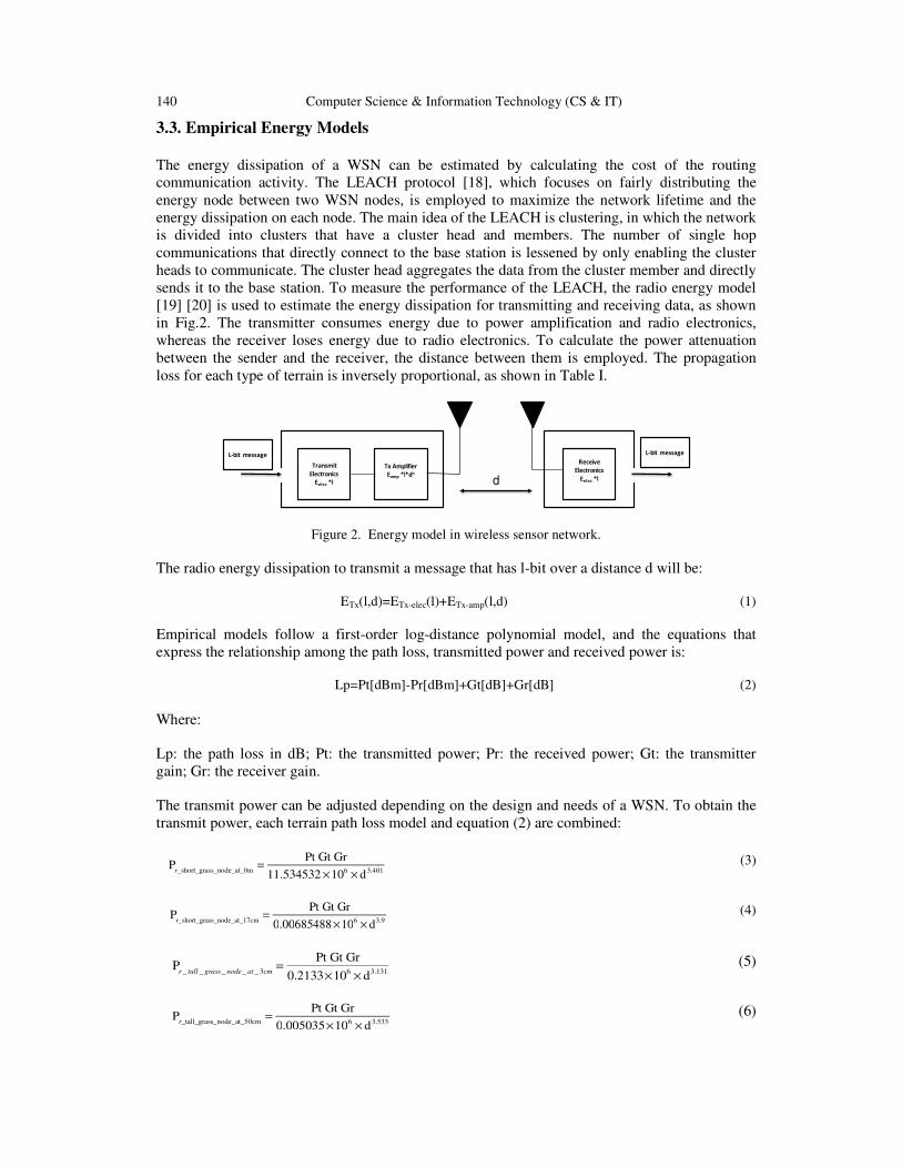
140 Computer Science & Information Technology (CS & IT)
3.3. Empirical Energy Models
The energy dissipation of a WSN can be estimated by calculating the cost of the routing
communication activity. The LEACH protocol [18], which focuses on fairly distributing the
energy node between two WSN nodes, is employed to maximize the network lifetime and the
energy dissipation on each node. The main idea of the LEACH is clustering, in which the network
is divided into clusters that have a cluster head and members. The number of single hop
communications that directly connect to the base station is lessened by only enabling the cluster
heads to communicate. The cluster head aggregates the data from the cluster member and directly
sends it to the base station. To measure the performance of the LEACH, the radio energy model
[19] [20] is used to estimate the energy dissipation for transmitting and receiving data, as shown
in Fig.2. The transmitter consumes energy due to power amplification and radio electronics,
whereas the receiver loses energy due to radio electronics. To calculate the power attenuation
between the sender and the receiver, the distance between them is employed. The propagation
loss for each type of terrain is inversely proportional, as shown in Table I.
Transmit
Electronics
Eelec *l
Tx Amplifier
Eamp *l*dn
Receive
Electronics
Eelec *l
L-bit message L-bit message
d
Figure 2. Energy model in wireless sensor network.
The radio energy dissipation to transmit a message that has l-bit over a distance d will be:
ETx(l,d)=ETx-elec(l)+ETx-amp(l,d) (1)
Empirical models follow a first-order log-distance polynomial model, and the equations that
express the relationship among the path loss, transmitted power and received power is:
Lp=Pt[dBm]-Pr[dBm]+Gt[dB]+Gr[dB] (2)
Where:
Lp: the path loss in dB; Pt: the transmitted power; Pr: the received power; Gt: the transmitter
gain; Gr: the receiver gain.
The transmit power can be adjusted depending on the design and needs of a WSN. To obtain the
transmit power, each terrain path loss model and equation (2) are combined:
Pr_short_grass_node_at_0m
=Pt Gt Gr
11.534532 ×10⁶ × d3.401
(3)
Pr_short_grass_node_at_17cm
=Pt Gt Gr
0.00685488 ×10⁶ × d3.9
(4)
Pr _ tall _ grass_ node_ at _ 3cm
=Pt Gt Gr
0.2133×10⁶ × d
3.131 (5)
Pr_tall_grass_node_at_50cm
=Pt Gt Gr
0.005035×10⁶ × d3.533
(6)

Computer Science & Information Technology (CS & IT) 141
Pr_dense_tree_node_at_0m
=Pt Gt Gr
0.167 ×10⁶ × d2.811 (7)
Pr_dense_tree_node_at_0m
=Pt Gt Gr
3.162 ×10⁶ × d3.274 (8)
The amplifying energy on the transmitter side depends on two factors: receiver sensitivity and
noise figure. To obtain the minimum transmitted power, a backward process is performed starting
from the power threshold to ensure that the received power must be higher than the threshold.
Multiplying the bit rate by the transmit energy per bit will generate transmit power and by
inputting the value of amplifying energy for each type of terrain:
Pt =
Eshort_grass_0_amp
Rbd
3.401
Eshort_grass_17_amp
Rbd
3.9
Etall_grass_3_amp
Rbd
3.131
Etall_grass_50_amp
Rbd
3.53
Edense_tree_0_amp
Rbd
2.81
Edense_tree_50_amp
Rbd
3.274
(9)
The received power can be obtained using the empirical channel propagation models from the
previous section:
Pr =
Eshort_grass_0_amp
RbG
tG
r
11.535×10⁶
Eshort_grass_17_amp
RbG
tG
r
0.0069 ×10⁶
Etall_grass_3_amp
RbG
tG
r
0.2133×10⁶
Etall_grass_50_amp
RbG
tG
r
0.005×10⁶
Edense_tree_0_amp
RbG
tG
r
0.167 ×10⁶
Edense_tree_50_amp
RbG
tG
r
3.162 ×10⁶
(10)
The received power can be obtained using the empirical channel propagation models from the
previous section:
Eshort_grass_0_amp
=P
r−thresh×11.535×10⁶
Rb
× Gt× G
r
(11)
Eshort_grass_17_amp
=P
r−thresh× 0.0069 ×10⁶
Rb
× Gt× G
r
(12)
Etall_grass_3_amp
=P
r−thresh× 0.2133×10
6
Rb
× Gt× G
r
(13)
Etall_grass_50_amp
=P
r−thresh× 0.005×10⁶
Rb
× Gt× G
r
(14)

142 Computer Science & Information Technology (CS & IT)
Edense_tree_0_amp
=P
r−thresh× 0.167 ×10
6
Rb
× Gt× G
r
(15)
Edense_tree_50_amp
=P
r−thresh× 3.162 ×10⁶
Rb
× Gt× G
r
(16)
The following formula is used to calculate the receiver threshold:
Pr-thresh[dBm]= 10log(KTB)+ F[dB]+ C/N[dB] (17)
where:
K: Boltzmann's constant; T: Absolute temperature in Kelvins; KT≈ 4*10-18 mW/Hz; B:
Bandwidth of the signal in Hz; F: Noise figure of the receiver; C/N: Signal-to-noise ratio.
To successfully receive a packet, the received power must be higher than -94 dBm. The dissipated
energy for each bit in the transceiver electronics is set to 50 nJ/bit. By adding the values in this
experiment (Gt=Gr=1.86 dB, ht=hr=5 cm, Rb=1 Mbps), the amplifying energy for each type of
terrain would be:
Eshort_grass_0_amp = 1.949pJ/bit/ m3.401
(18)
Eshort_grass_17_amp = 1.158pJ/bit/ m3.9
(19)
Etall_grass_3_amp = 0.036pJ/bit/ m3.131
(20)
Etall_grass_50_amp= 0.851fJ/bit/ m3.533
(21)
Edense_tree_0_amp= 0.0282pJ/bit/ m2.811
(22)
Edense_tree_50_amp= 0.5344pJ/bit/ m3.27
(23)
A comparison with well-known theoretical propagation models was performed to show the effect
of real environment terrains on a WSN. The impact of free space and two-ray propagation models
on WSN performance are compared with the performance of all empirical models. This effect
drives the energy models, and using the parameters in this experiment, the energy models would
be:
Efree_space_amp= 1.10fJ/bit/ m2
(24)
Etwo-ray_amp= 0.0013pJ/bit/ m4
(25)
3.4. Node Connectivity
The connectivity of a network measures how well the nodes in a network are connected within
the deployed area. The connection between two wireless nodes comprise either a direct link or an
indirect link. To define a communication link between two nodes n1(x1,y1) and n2 (x2,y2), the
Euclidean distance d between them is calculated.
d(n1,n
2) = (x
1− x
2)2 + ( y
2− y
1)2 (26)

Computer Science & Information Technology (CS & IT) 143
If the Euclidean distance between the two nodes is less than the communication range, it is
defined as a directly connected node. For these nodes, the maximum transmission range
determined by the empirical RF propagation model of a specific environment will determine the
connectivity between these nodes.
dshort _ grass_ node_ at _0m
= (P
tG
tG
r
11.534532 ×10⁶ × Pr−thresh
)1
3.401 (27)
dshort _ grass_ node_ at _17cm
= (P
tG
tG
r
0.00685488 ×10⁶ × Pr−thresh
)1
3.9 (28)
dtall _ grass_ node_ at _3cm
= (P
tG
tG
r
0.2133×10⁶ × Pr −thresh
)1
3.131 (29)
dtall _ grass_ node_ at _50cm
= (P
tG
tG
r
0.005035×10⁶ × Pr−thresh
)1
3.533 (30)
ddense _ tree _ node_ at _ 0m
= (P
tG
tG
r
0.167 ×10⁶ × Pr−thresh
)1
2.811 (31)
ddense_ tree_ node_ at _50cm
= (P
tG
tG
r
11.534532 ×10⁶ × Pr−thresh
)1
3.274 (32)
The connectivity matrix is used to evaluate an entire network’s connectivity. The matrix has the
size of n * n, where n is the number of nodes in the network. Based on the radio range and the
distance between the nodes, the matrix element will have a value of 1 if they are connected and a
value of 0 if they are not connected. The indirect links between the nodes are calculated by
scanning all nodes to identify indirect nodes between the previous two nodes. The connectivity
percentage is calculated when the connectivity matrix is ready. The framework checks the
connectivity among all nodes on each LEACH round and shows the variation in the connectivity
for the surviving nodes.
3.5. Region of Interest Coverage
Coverage is one of the most important metrics that measures the deployment effectiveness and
the quality of service of a WSN. Coverage indicates the number of points in the deployment area
that are covered by the deployed sensors. The binary disc sensing model is adapted to compute
the average. The sensing area is the circle that surrounds a sensor with the radius r, which is equal
to the sensing range of the sensor. Each point that does not fall within this radius is considered to
be an uncovered point. The sensing range is assumed to be the same for each sensor and can be
determined as an input.
Cxy
Si( ) =
1: if d Si, P( ) ≤ r
0 : otherwise
(33)
where Si is the sensor node position, P is the position of any node in the area, and r is the sensing
range. The distance between the node and the point is calculated using the Euclidean distance
equation. The percentage of coverage is given by:
Coverage =c
p∈P1∑
×100 (34)

144 Computer Science & Information Technology (CS & IT)
The framework checks the change in coverage on each round due to the change in the remaining
number of nodes.
4. DEPLOYMENT ANALYSIS
In this section, the holistic performance of stochastic and deterministic deployment is analyzed
for all terrains. The provided results support decision-making processes by studying the impact of
several factors that influence the WSN performance. MATLAB is used to implement and analyze
the deployment. The following section shows the analysis of the simulation output, where the
deployment area is a rectangle with a size of 200 m X 200 m. The base station is located at 100 m
X 205 m. Four common deployments tested with the same variables were applied to all
environments to estimate the coverage, connectivity, lifetime, and throughput. The data packet
has 6400 bits, and the control packets have 200 bits. The number of cluster heads for each round
is 5% of the total number of remaining nodes. The initial energy is the same for all nodes, which
is 2 joules. The holistic performance of the network was tested with a variable number of nodes
and sensing ranges.
4.1. Lifetime
Using the presented framework, the lifetime is computed and simulated, and the results are
presented in Figures 3-6.
0 1000 2000 3000 4000 5000 6000 7000 8000 9000 10000
Round
0
10
20
30
40
50
60
70
80
90
100
Nu
mb
er
of
de
ad
no
de
s
Network Lifetime
Free Space Model
Two-ray Model
Dense Tree Model at 50cm
Dense Tree Model at 0m
Short Grass Model at 0m
Short Grass Model at 17cm
Tall Grass Model at 3cm
Tall Grass Model at 50cm
Figure 3. Lifetime of random deployment in rounds for all terrains.
0 1000 2000 3000 4000 5000 6000 7000 8000 9000 10000
Round
0
20
40
60
80
100
120
Num
ber
of dead n
odes
Network Lifetime
Free Space Model
Two-Ray Model
Dense Tree Model at 50cm
Dense Tree Model at 0m
Short Grass Model at 0m
Short Grass Model at 17cm
Tall Grass Model at 3cm
Tall Grass Model at 50cm
Figure 4. Lifetime of triangular deployment in rounds for all terrains.

Computer Science & Information Technology (CS & IT) 145
0 1000 2000 3000 4000 5000 6000 7000 8000 9000 10000
Round
0
10
20
30
40
50
60
70
80
90
100
Num
ber of dead n
odes
Network Lifetime
Free Space Model
Two-Ray Model
Dense Tree Model at 50cm
Dense Tree Model at 0m
Short Grass Model at 0m
Short Grass Model at 17cm
Tall Grass Model at 3cm
Tall Grass Model at 50cm
Figure 5. Lifetime of square deployment in rounds for all terrains.
0 1000 2000 3000 4000 5000 6000 7000 8000 9000 10000
Round
0
20
40
60
80
100
120
Num
ber
of dead n
odes
Network Lifetime
Free Space Model
Two-Ray Model
Dense Tree Model at 50cm
Dense Tree Model at 0m
Short Grass Model at 0m
Short Grass Model at 17cm
Tall Grass Model at 3cm
Tall Grass Model at 50cm
Figure 6. Lifetime of hexagonal deployment in rounds for all terrains.
The results of simulating the propagation models of different environments with different
deployments show a significant difference between the theoretical propagation model and the
empirical propagation model. Placing nodes on the ground in a dense tree environment yields the
longest network lifetime, whereas setting the nodes over the ground (height of seventeen cm) in a
short grass environment yields the lowest lifetime. The first node dies in the dense tree
environment at 3519 rounds with 62025 total packets sent to the base station. This finding is
lower than the results received from the free space model. For short grass with the nodes spaced
at a height of 17 cm, the first node dies in the third round with only 31 packets sent to the base
station from the entire network. The significant variations in the lifetime of the network are
caused by the path loss exponent of each terrain. The dense tree environment has a path loss
exponent of 2.81, which is the lowest path loss exponent among all terrains, whereas the short
grass environment has the highest path loss exponent of 3.9. The lifetime is stable for all terrains,
even if the number of nodes is increased; however, it gradually decreases with the random
deployment. Stochastic and deterministic deployments have the highest lifetime with 50 to 100
nodes. Placing the nodes on the ground among a dense tree environment ensures the longest
network lifetime, whereas setting the nodes over the ground in a short grass environment
produces the lowest lifetime. The number of dead nodes becomes stable with 60 to 80 nodes for
most terrains for all deployments. The lifetime is the highest with random deployments compared
to other deployment options. All deterministic deployment nodes have a lower lifetime due to the

146 Computer Science & Information Technology (CS & IT)
required distance between two nodes to cover all regions of interest. This arbitrary distance
causes the data transmission cost to exceed the random deployment.
4.2. Connectivity
The results obtained from the framework are presented in the following figures.
0 1000 2000 3000 4000 5000 6000 7000 8000 9000 10000
Lifetime (Round)
0
0.1
0.2
0.3
0.4
0.5
0.6
0.7
0.8
0.9
1
Co
nn
ec
tiv
ity
(%
)
Deployment Connectivity
Free Space Model
Two-Ray Model
Dense Tree Model at 50cm
Dense Tree Model at 0m
Short Grass Model at 0m
Short Grass Model at 17cm
Tall Grass Model at 3cm
Tall Grass Model at 50cm
Figure 7. Connectivity of random deployment for all terrains.
0 1000 2000 3000 4000 5000 6000 7000 8000 9000 10000
Round
0
0.1
0.2
0.3
0.4
0.5
0.6
0.7
0.8
0.9
1
Co
nn
ect
ivit
y (%
)
Network Connectivity
Free Space Model
Two-Ray Model
Dense Tree Model at 50cm
Dense Tree Model at 0m
Short Grass Model at 0m
Short Grass Model at 17cm
Tall Grass Model at 3cm
Tall Grass Model at 50cm
Figure 8. Connectivity of triangular deployment for all terrains.
0 1000 2000 3000 4000 5000 6000 7000 8000 9000 10000
Round
0
0.1
0.2
0.3
0.4
0.5
0.6
0.7
0.8
0.9
1
Co
nn
ec
tiv
ity
(%
)
Network Connectivity
Free Space Model
Two-ray Model
Dense Tree Model at 50cm
Dense Tree Model at 0m
Short Grass Model at 0m
Short Grass Model at 17cm
Tall Grass Model at 3cm
Tall Grass Model at 50cm
Figure 9. Connectivity of square deployment for all terrains.

Computer Science & Information Technology (CS & IT) 147
0 1000 2000 3000 4000 5000 6000 7000 8000 9000 10000
Round
0
0.1
0.2
0.3
0.4
0.5
0.6
0.7
0.8
0.9
1
Co
nn
ec
tivit
y (
%)
Network Connectivity
Free Space Model
Two-Ray Model
Dense Tree Model at 50cm
Dense Tree Model at 0m
Short Grass Model at 0m
Short Grass Model at 17cm
Tall Grass Model at 3cm
Tall Grass Model at 50cm
Figure 10. Connectivity of hexagonal deployment for all terrains.
Figures 7-10 represent the connectivity over all terrains with stochastic and deterministic
deployments. The theoretical free space model, model of dense tree terrain at 50 cm, and model
of tall grass terrain at 50 cm have the highest connectivity, whereas all other terrains have low
connectivity for the majority of deployment choices. This finding is attributed to the low median
path loss at the reference distance. The dense tree model with a height of zero meters has a high
connectivity with square and triangular deployments due to the distance between two nodes,
which is enables a high connectivity. For all terrains, the connectivity percentage decreases after
few rounds due to the high number of nodes that have died. Square and hexagonal deployments
attain a high connectivity level with 50 to 100 nodes. To optimize the connectivity of random
deployments, nearly 150 to 200 nodes are needed. The triangular deployment has the lowest cost
due to the small number of nodes that are required to obtain a high level of connectivity.
4.3. Coverage The following figures illustrate the amount of coverage that is provided by each deployment and
the change in the coverage percentage over the network lifetime for each terrain.
0 1000 2000 3000 4000 5000 6000 7000 8000 9000 10000
Round
0
0.1
0.2
0.3
0.4
0.5
0.6
0.7
0.8
0.9
1
Co
ve
rag
e (
%)
Deployment Coverage
Free Space Model
Two-ray Model
Dense Tree Model at 50cm
Dense Tree Model at 0m
Short Grass Model at 0m
Short Grass Model at 17cm
Tall Grass Model at 3cm
Tall Grass Model at 50cm
Figure 11. Change in coverage for all terrains with random deployment.

148 Computer Science & Information Technology (CS & IT)
0 1000 2000 3000 4000 5000 6000 7000 8000 9000 10000
Round
0
0.1
0.2
0.3
0.4
0.5
0.6
0.7
0.8
0.9
1
Co
vera
ge
(%
)
Network Coverage
Free Space Model
Two-Ray Model
Dense Tree Model at 50cm
Dense Tree Model at 0m
Short Grass Model at 0m
Short Grass Model at 17cm
Tall Grass Model at 3cm
Tall Grass Model at 50cm
Figure 12. Change in coverage for all terrains with triangular deployment.
0 1000 2000 3000 4000 5000 6000 7000 8000 9000 10000
Round
0
0.1
0.2
0.3
0.4
0.5
0.6
0.7
0.8
0.9
1
Co
vera
ge
(%
)
Network Coverage
Free Space Model
Two-Ray Model
Dense Tree Model at 50cm
Dense Tree Model at 0m
Short Grass Model at 0m
Short Grass Model at 17cm
Tall Grass Model at 3cm
Tall Grass Model at 50cm
Figure 13. Change in coverage for all terrains with square deployment.
0 1000 2000 3000 4000 5000 6000 7000 8000 9000 10000
Round
0
0.1
0.2
0.3
0.4
0.5
0.6
0.7
0.8
0.9
1
Co
vera
ge
(%
)
Network Coverage
Free Space Model
Two-Ray Model
Dense Tree Model at 50cm
Dense Tree Model at 0m
Short Grass Model at 0m
Short Grass Model at 17cm
Tall Grass Model at 3cm
Tall Grass Model at 50cm
Figure 14. Change in coverage for all terrains with hexagonal deployment.
Figures 11 to 14 illustrate the coverage in the region of interest, which is defined by at least 35
nodes for hexagonal deployment, 52 nodes for triangular deployment, 50 nodes for random
deployment, and 56 nodes for square deployment, respectively. They deploy with a variable
sensing range for each of the deployments starting from 5 m to 30 m. With a 10- to 15-meter
sensing range, the triangular deployment achieves almost full coverage in the region of interest.
Square deployment can provide similar coverage with a few additional nodes. For each
deployment choice, the region of interest can be covered with a high sensing range: 30 m for
random deployment, 25 m for triangular and square deployment, and more than 30 m for
hexagonal deployment. Hexagonal deployment utilizes the highest number of nodes, followed by
square, triangular, and random deployments. However, random deployment seems inefficient due
to its defined number of nodes that are randomly stationed. An analysis of the applied techniques
applied shows that the hexagonal technique has the largest number of nodes. However, triangular
deployment is the best pattern regarding efficiency within the same region.
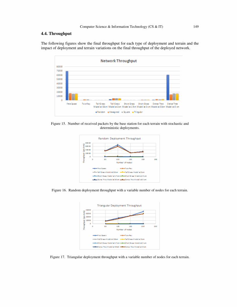
Computer Science & Information Technology (CS & IT) 149
4.4. Throughput
The following figures show the final throughput for each type of deployment and terrain and the
impact of deployment and terrain variations on the final throughput of the deployed network.
Figure 15. Number of received packets by the base station for each terrain with stochastic and
deterministic deployments.
Figure 16. Random deployment throughput with a variable number of nodes for each terrain.
Figure 17. Triangular deployment throughput with a variable number of nodes for each terrain.

150 Computer Science & Information Technology (CS & IT)
0
10000
20000
30000
40000
0 50 100 150 200 250
Th
rou
gh
pu
t (p
ack
ets
)
Number of nodes
Square Deployment Throughput
Free Space Two-Ray
Tall Grass Model at 50cm Tall Grass Model at 3cm
Short Grass Model at 17cm Short Grass Model at 0 cm
Dense Tree Model at 50cm Dense Tree Model at 0 cm
Figure 18. Square deployment throughput with a variable number of nodes for each terrain.
0
10000
20000
30000
40000
0 50 100 150 200
Th
rou
gh
pu
t (p
ack
ets
)
Number of nodes
Hexagonal Deploymant Throughput
Free Space Two-Ray
Tall Grass Model at 50cm Tall Grass Model at 3cm
Short Grass Model at 17cm Short Grass Model at 0 cm
Dense Tree Model at 50cm Dense Tree Model at 0 cm
Figure 19. Hexagonal deployment throughput with a variable number of nodes for each terrain.
Figures 15-19 represent the network throughput after ten thousand rounds, which shows the
number of packets that has been successfully received by the base station. As illustrated in the
figures, the random deployment has the highest throughput compared with other deployments.
For all deterministic deployments, the throughput increases by adding nodes and decreases in the
random deployment for more than 100 nodes. Most of the terrains produce a throughput that is
similar to the throughput of the theoretical two-ray model. However, they have a low throughput
compared with the dense tree model with the nodes on the ground, which is similar to the free
space model. With the exception of the dense tree model with the node on the ground, the impact
of the deployments, either random or deterministic, among these choices is similar.
5. CONCLUSIONS AND FUTURE WORK This paper presents a realistic deployment framework that investigates WSN performance for
several stochastic and deterministic deployments. The study shows that deterministic deployment
is not the optimum solution when considering a holistic viewpoint, as shown in the literature
review. A trade-off exists among selecting the optimum coverage, connectivity, lifetime, and
throughput. This study investigates the impact of empirical propagation models on WSN
performance. Table 3 summarizes the deployment options and shows the best choice of
deployment option for each number of nodes from 50 nodes to 200 nodes. The empirical
propagation model was utilized for dense trees, tall grass, and short grass with different heights to
devise an accurate performance analysis that considers the surrounding environment. The
findings of this study indicate that theoretical propagation models are not precise in determining
WSN performance and the evaluation of WSN performance should include empirical propagation
models. The findings of this research will support deployment decision makers due to its focus on
the impact of real environments and the deployment choices that can be applied in the pre-
deployment stage to predict and optimize the deployment efficiency. Future research will focus

Computer Science & Information Technology (CS & IT) 151
on optimizing the simulation framework by incorporating artificial intelligence and prediction
methods. Determining the optimum number of nodes to be deployed for each terrain and their
locations is an open issue to further investigation. Additional stochastic deployments need to be
included and analyzed. In addition, the impact of deployment and terrain needs to be explored
with additional routing protocols. The scope of future research should be expanded to determine
the performance of multi-terrain environments.
Table 1. Holistic Performance Summary for Stochastic and Deterministic Deployments.
Performance Number of nodes Random Square Hexagonal Triangular
Throughput
50 √
100 √
150 √ √
200 √
Lifetime
50 √
100 √
150 √ √
200 √
Coverage
50 √
100 √
150 √
200 √ √
Connectivity
50 √
100 √
150 √
200 √
REFERENCES
[1] I. F. Akyildiz and M. C. Vuran, Wireless Sensor Networks, no. 1. 2010.
[2] M. R. Senouci and A. Mellouk, Deploying wireless sensor networks : theory and practice. 2016.
[3] A. AlSayyari, I. Kostanic, and C. E. Otero, “An Empirical Path Loss Model for Wireless Sensor
Network Deployment in an Artificial Turf Environment,” Proc. 11th IEEE Int. Conf. Networking,
Sens. Control, pp. 637–642, 2014.
[4] T. O. Olasupo, C. E. Otero, K. O. Olasupo, and I. Kostanic, “Empirical path loss models for wireless
sensor network deployments in short and tall natural grass environments,” IEEE Trans. Antennas
Propag., vol. 64, no. 9, pp. 4012–4021, 2016.
[5] C. E. Otero, I. Kostanic, and L. D. Otero, “Development of a simulator for stochastic deployment of
wireless sensor networks,” J. Networks, vol. 4, no. 8, pp. 754–762, 2009.
[6] W. Y. Poe and J. B. Schmitt, “Node deployment in large wireless sensor networks,” Asian Internet
Eng. Conf. - AINTEC ’09, pp. 77–84, 2009.
[7] R. Ricardo, H. G. Xiong, Q. Gao, A. Magallanes, and F. Candilio, “Monte Carlo Analysis of nodes
deployment for large-scale Wireless Sensor Network using range-free location methods,” Proc. - 2010
IEEE 2nd Symp. Web Soc. SWS 2010, pp. 484–489, 2010.
[8] T. HAYAJNEH and S. KHASAWNEH, “Analysis and Evaluation of Random Placement Strategies in
Wireless Sensor Networks,” J. Circuits, Syst. Comput., vol. 23, no. 10, p. 1450138, 2014.

152 Computer Science & Information Technology (CS & IT)
[9] Y. Bai, J. Li, Q. Han, Y. Chen, and D. Qian, “Research on Planning and Deployment Platform for,” in
Advances in Grid and Pervasive Computing, 2007, pp. 738–743.
[10] C. E. Otero, I. Kostanic, A. Peter, A. Ejnioui, and L. Daniel Otero, “Intelligent system for predicting
wireless sensor network performance in on-demand deployments,” 2012 IEEE Conf. Open Syst.
ICOS 2012, 2012.
[11] S. P. Shaktawat and O. Sharma, “Node Deployment Models and their Performance Parameters for
Wireless Sensor Network : A Perspective,” Int. J. Comput. Appl., vol. 88, no. 9, pp. 1–6, 2014.
[12] S. Nouh, R. A. Abbass, D. A. El Seoud, N. A. Ali, R. M. Daoud, H. H. Amer, and H. M. ElSayed,
“Effect of node distributions on lifetime of Wireless Sensor Networks,” IEEE Int. Symp. Ind.
Electron., pp. 434–439, 2010.
[13] R. Atiq Ur, H. Hasbullah, and S. Najm Us, “Impact of Gaussian deployment strategies on the
performance of wireless sensor network,” vol. 2, pp. 771–776, 2012.
[14] N. A. Ali and O. A. Nasr, “WSN lifetime prolongation for deterministic distributions using a
hierarchical routing protocol,” IEEE AFRICON Conf., 2013.
[15] S. M. and S. B. Ram Shringar Raw, Shailender Kumar, “Comparison and Analysis of Node
Deployment for Efficient Coverage in Sensor Network,” in Intelligent Computing, Networking, and
Informatics. Advances in Intelligent Systems and Computing, 2014, vol. 243, pp. 1047–1054.
[16] The Office of Naval Research (ONR), “Intelligence, Surveillance and Reconnaissance (ISR) Thrust
Area.” [Online]. Available: https://www.onr.navy.mil/en/Science-Technology/Departments/Code-
30/All-Programs/ONR_30_Contacts.
[17] C. E. Otero, R. Haber, A. M. Peter, A. Alsayyari, and I. Kostanic, “A Wireless Sensor Networks’
Analytics System for Predicting Performance in On-Demand Deployments,” IEEE Syst. J., vol. 9, no.
4, pp. 1344–1353, 2015.
[18] W. B. Heinzelman, A. P. Chandrakasan, and H. Balakrishnan, “An application-specific protocol
architecture for wireless microsensor networks,” IEEE Trans. Wirel. Commun., vol. 1, no. 4, pp. 660–
670, 2002.
[19] Wendi B. Heinzelman, “Application-specific protocol architectures for wireless networks,” 2000.
[20] A. Aldosary and I. Kostanic, “The impact of tree-obstructed propagation environments on the
performance of wireless sensor networks,” in 2017 IEEE 7th Annual Computing and Communication
Workshop and Conference, CCWC 2017, 2017, pp. 1–7.
AUTHORS
Amar Jaffar was born in Makkah, Saudi Arabia in 1984. He received the B.S.
degree in computer engineering from Umm Al Qura University, Makkah, Saudi
Arabia, in 2006 and the M.S. degree in electrical engineering from University of
New Haven, New Haven, USA, in 2012. He is currently pursuing the Ph.D. degree
in Computer Engineering at Florida Institute of Technology. From 2007 to 2010, he
is a lecturer in Computer Engineering Department at Umm Al-Qura University,
Makkah, KSA. His research interests WSN deployment, wireless multimedia sensor
networks routing, Internet of things, network security and system-on-chip.

Computer Science & Information Technology (CS & IT) 153
Carlos Enrique Otero (SM’09) was born in Bayamon, Puerto Rico, in 1977. He
received the B.S. degree in computer science, the M.S. degree in software engineering,
the M.S. degree in systems engineering, and the Ph.D. degree in computer engineering
from Florida Institute of Technology, Melbourne. He is currently Associate Professor
and the Co-Director of the Wireless Center of Excellence, Florida Institute of
Technology. He was an Assistant Professor with the University of South Florida and
the University of Virginia at Wise. He has authored over 70 papers in wireless sensor
networks, Internet-of-Things, big data, and hardware/software systems. His research
interests include the performance analysis, evaluation, and optimization of computer
systems, including wireless ad hoc and sensor networks. He has over twelve years of industry experience in
satellite communications systems, command and control systems, wireless security systems, and unmanned
aerial vehicle systems.

AUTHOR INDEX
Ali Al-Ataby 85
Amakata Masazumi 55
Amar Jaffar 135
Bakhous H 99
Binxing Fang 113, 123
Carlos E. Otero 135
Cina Motamed 73
Eugene C. Ezin 73
Fatemah Alghamedy 21, 37
Fujii Junichiro 55
Jinyu Shi 113
Josky Aïzan 73
Jun Zhang 21, 37
Lagmiri S.N 99
Maryam Al-Ghamdi 21
Mohammed M. Alammar 85
Qiang Ruan 113, 123
Shimamoto Yuri 55
Wassim Kabbara 01
Xinchun Yang 01
Yasuno Takato 55
Yu Han 123
Yue Wu 113
Zhongru Wang 113, 123


![Figure 6(a). Conceptual diagram illustrating vector quantization … · 2016-11-07 · GMM based Speaker Recognition. [9] Mahdi Shaneh, and Azizollah Taheri., Voice Command Recognition](https://static.documents.pub/doc/80x56/5f082f1c7e708231d420c1b5/figure-6a-conceptual-diagram-illustrating-vector-quantization-2016-11-07-gmm.jpg)
