Computer Science Technical Report TR-11-04 April 20, 2011 Joe Hays, Adrian Sandu, Corina Sandu, Dennis Hong “Motion Planning of Uncertain Ordinary Differential Equation Systems” Center for Vehicle Systems and Safety Computer Science Department & Department of Mechanical Engineering Virginia Polytechnic Institute and State University Blacksburg, VA 24061 Phone: (540)-231-2193 Fax: (540)-231-9218 Email: [email protected]Web: http://www.eprints.cs.vt.edu
Transcript
Computer Science Technical Report
TR-11-04
April 20, 2011
Joe Hays, Adrian Sandu, Corina Sandu, Dennis Hong
“Motion Planning of Uncertain Ordinary Differential
Equation Systems”
Center for Vehicle Systems and Safety
Computer Science Department & Department of Mechanical
Engineering
Virginia Polytechnic Institute and State University
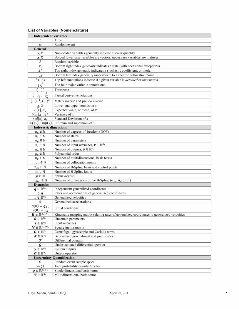
General , Non-bolded variables generally indicate a scalar quantity , Bolded lower case variables are vectors, upper case variables are matrices Random variable Bottom right index generally indicates a state (with occasional exceptions). Top right index generally indicates a stochastic coefficient, or mode. Bottom left index generally associates to a specific collocation point. , Top left annotations indicate if a given variable is actuated or unactuated. The four major variable annotations Transpose , Partial derivative notations , # Matrix inverse and pseudo inverse , Lower and upper bounds on , Expected value, or mean, of , Variance of !", Standard Deviation of #$%, !&' Infimum and supremum of
Indexes & dimensions $( ∈ ℕ Number of degrees-of-freedom (DOF) $+ ∈ ℕ Number of states $, ∈ ℕ Number of parameters $ ∈ ℕ Number of input wrenches, - ∈ ℝ/0 $1 ∈ ℕ Number of outputs, 2 ∈ ℝ/3 '1 ∈ ℕ Polynomial order $4 ∈ ℕ Number of multidimensional basis terms $5, ∈ ℕ Number of collocation points $+, ∈ ℕ Number of B-Spline basis and control points 6 ∈ ℕ Number of B-Spline knots 7 ∈ ℕ Spline degree $(8 ∈ ℕ Number of dimensions of the B-Spline (e.g., $( or $) Dynamics : ∈ ℝ/; Independent generalized coordinates :< , := Rates and accelerations of generalized coordinates > ∈ ℝ/; Generalized velocities >< Generalized accelerations :? = :A ,
>? = >A Initial conditions B ∈ ℝ/C×/C Kinematic mapping matrix relating rates of generalized coordinates to generalized velocities E ∈ ℝ/F Uncertain parameters - ∈ ℝ/0 Input wrenches G ∈ ℝ/C×/C Square inertia matrix H ∈ ℝ/C Centrifugal, gyroscopic and Coriolis terms I ∈ ℝ/C Generalized gravitational and joint forces J Differential operator K Under-actuated differential operator 2 ∈ ℝ/3 System outputs L ∈ ℝ/3 Output operator
Uncertainty Quantification Ω Random event sample space N Joint probability density function O ∈ ℝ,3PQ Single dimensional basis terms Ψ ∈ ℝ/S Multidimensional basis terms
Hays, Sandu, Sandu, Hong April 20, 2011 3
T, T ∈ ℝ/UF Kth collocation point , ∈ ℝ/UF Kth intermediate variable of the ith state representing expanded quantity V ∈ ℝ/S×/UF Collocation matrix
Nonlinear Programming minZ Optimization objective through manipulation of Z Z List of manipulated variables J Scalar objective function z Scalarlization weights for the individual input wrench contributions
tf Final time of trajectories ] Inequality constraints (typically bounding constraints) ^ B-Spline curve _,7 B-Spline basis terms of degree 7 and # = 1 … $+, b = cde B-Spline control points where # = 1 … $+, bf = cd′e Derived control points for velocity B-Splines where # = 1 … $+, bff = cd′′e Derived control points for acceleration B-Splines where # = 1 … $+, h, A signed minimum distance between two geometric bodies i and j
1 INTRODUCTION
1.1 MOTIVATION
Design engineers cannot quantify exactly every aspect of a given system. These uncertainties frequently create difficulties in
accomplishing design goals and can lead to poor robustness and suboptimal performance. Tools that facilitate the analysis and
characterization of the effects of uncertainties enable designers to develop more robustly performing systems. The need to
analyze the effects of uncertainty is particularly acute when designing motion plans for dynamical systems. Frequently, engineers
do not account for various uncertainties in their motion plan in order to save time and to reduce costs. However, this simply
delays, or hides, the cost which is inevitably incurred down-stream in the design flow; or worse, after the system has been
deployed and fails to meet the design goals. Ultimately, if a robust motion plan is to be achieved, uncertainties must be accounted
for up-front during the design process.
Many industries employ dynamic systems with planned motions that operate with uncertainty. For example, the industrial
manufacturing sector uses articulated robotic systems for repeated tasks such as welding, packaging, and assembly (see Figure
1.1); medical robots are now being designed to aid physicians in surgery; and autonomous vehicles are taking on more and more
tasks in military, municipality, and even domestic operations.
http://img.directindustry.com
http://www.drives.co.uk
Figure 1.1—Industrial robots are example applications of engineered systems whose robustness and
performance can be improved by the proper treatment of uncertainty during the motion planning process.
In the area of unmanned ground vehicles (UGVs), organizations such as the Defense Advanced Research Projects Agency
(DARPA), the National Science Foundation (NSF), Office of Naval Research (ONR), and other agencies continue to investigate
the application of legged robotic systems. Additionally, many UGVs, unmanned surface vehicles (USVs), and unmanned
underwater vehicles (UUV’s) are outfitted with articulated accessories to perform various tasks. These systems are planned to aid
in diverse operations including Improvised Incendiary Device (IID) detection and disarmament, material and equipment handling
and convoy, search and rescue. Three show-case examples include: Boston Dynamics’ BigDog and next generation LS3 robots,
who aid in the convoy of soldier equipment with an unknown weight in harsh rugged terrain; Vecna’s BEAR robot aids in the
retrieval of wounded soldiers of varying size and weight also in uncertain terrain. These examples clearly illustrate the need to
design motion strategies with uncertainties in mind. Elaborating further on the equipment convoy task, optimal design of the
locomotion strategy, or gait, of the systems carrying uncertain payloads could result in large fuel/energy savings as well as
lengthen achievable distances of a given convoy operation (see Figure 1.2).
Hays, Sandu, Sandu, Hong April 20, 2011 4
http://www.bostondynamics.com
http://www.xconomy.com
Figure 1.2—Autonomous robotic systems illustrate multibody dynamic systems that operate within uncertain
environments and payloads.
These are a few showcase examples of specific dynamic system applications that would benefit if uncertainty was accounted
for during the motion planning process.
Another noteworthy application is in the area of studying and analyzing human performance measures. For example,
TARDEC [1-4] is actively investigating the effects of protective clothing and routine tasks of soldiers, such as: crawling,
walking, running, lifting, calisthenics and other human physiology aspects. The studies aim to quantify muscle stress/fatigue,
metabolic rates, and required strength of tasks expected of soldiers (see Figure 1.3); where techniques typically involve dynamic
analysis and various optimal motion planning formulations of virtual and physical humanoids. Recently the automotive
manufacturing sector is using similar analyses to ensure the designed assembly lines are safe for their employees [5]. Literature to
date has shown that these efforts currently assume a deterministic dynamic system model. Clearly soldiers and assembly line
workers operate with uncertain payloads and tasks, therefore, the ability to quantify and account for these uncertainties would
enrich these human performance studies.
http://www.ccad.uiowa.edu/vsr/
Figure 1.3—Optimization based human performance studies such as quantifying muscle stress/fatigue,
metabolic rates, and required strength can be enriched with the proper treatment of uncertainty.
1.2 STATE OF THE ART IN MOTION PLANNING AND UNCERTAINTY QUANTIFICATION
In the following, a review of the literature is presented where works related to motion planning and uncertainty quantification
are specifically covered.
1.2.1 Deterministic Optimization-Based Motion Planning In [6], Park presents a nonlinear programming approach to motion planning for robotic manipulator arms described by
deterministic ODEs. The main contribution of Park’s work is to define new cost terms that capture actuator force limiting
characteristics; where actuator velocities and resulting feasible torques are defined. Park’s formulation utilizes quintic B-Splines
to provide a tractable finite dimensional search space along with Quasi-Newton based solver methods (e.g. BFGS). Additionally,
he approaches obstacle avoidance by defining distance constraints with the growth function technique from [7].
Sohl, Martin, and Bobrow presented a series of papers that document their excellent work in the area of optimal manipulator
motions. At the heart of their work is the use of a novel geometric formulation of robot dynamics based on the differential
geometry principles of Lie Groups and Lie Algebras [8-10]. The approach provides a few critical properties that streamline the
optimal motion planning problem; first, the geometric dynamics formulation has an equivalent recursive formulation that
provides O(n) computational complexity; second, use of the Product-of-Exponentials (POE) in the formulation provides a
straight-forward approach to calculating the gradient of the optimal motion planning objective function. Access to an exact
analytic gradient improves the nonlinear programming solve by helping avoid premature convergence or excessive searching for
the frequently ill-conditioned motion planning problems. In [11], Martin and Bobrow present a minimum effort formulation for
open chain manipulators based on the recursive geometric dynamics. A detailed presentation for the recursive calculation of the
analytic objective function gradient is a major contribution of this work. They also use cubic B-Splines to provide a finite
dimensional search space. In [12], Sohl and Bobrow extend the work to address branched kinematic chains; in [13-15] they again
extend the work to address under-actuated manipulators; and in [16, 17] the methods are applied to the specific design problem of
Hays, Sandu, Sandu, Hong April 20, 2011 5
maximizing the weightlifting capabilities of a Puma 762 Robot. Throughout this series of work the sequential quadratic
programming (SQP) technique is used for the constrained optimization; however, in [18], a Newton type optimization algorithm
is developed that reuses the analytic gradient and hessian information from the geometric dynamics. In [19], Bobrow, Park, and
Sideris, further extend the work to solve infinite-dimensional problems using a sequence of linear-quadratic optimal control sub-
problems and cover minimum energy, control effort, jerk and time. Finally, in [20], Lee et. al. extend the geometric-based
optimization methods to more general dynamic systems including those with closed-kinematic loops and redundant actuators and
sensors.
Another inspiring body of research comes from Xiang, Abdel-Malek et. al. [2-4, 21-25] where analytic derivatives for the
optimization cost of general open, branched, and closed looped systems, described by recursive Lagrangian Dynamics, is
presented. Formulations are based on the Denavit-Hartenberg kinematic methods, cubic B-Splines, and SQP-based solvers.
Application emphasis focuses on the motion planning of over-actuated 3D human figures; where models with as many as 23
DOFs and 54 actuators are used to design natural cyclic walking gaits. A combination of inverse and forward dynamics
formulations are used, however, their formulation avoids explicit numerical integration (required in a sequential nonlinear
programming (SeqNLP) methodology). Instead, their formulation makes use of the simultaneous nonlinear programming
(SimNLP) methodology; which discretizes the EOMs over the trajectory of the system and treats the complete set of equations as
equality constraints for the NLP. Therefore, the SimNLP has a much larger set of constraints than the SimNLP approach, but,
enjoys a more structured NLP that typically experiences faster convergence. (Note: the definitions of SimNLP and SeqNLP come
from [26, 27].) Additional contributions of Xiang’s work include human walking specific constraint formulations.
In [28], Park and Park present a convex motion planning algorithm that determines a stable motion plan that approximates a
reference motion plan for a humanoid robotic system. The use case stems from applying measured joint trajectories from a
human and applying them to a humanoid robot; this generally results in an unstable reference trajectory for the robot. However,
Park and Park present a second-order cone formulated motion planning problem that determines a stable motion plan yet still
approximates the reference trajectory in a least-squares sense. Similar work was presented in [29], where reference motion plans
are refined online through use of a recursive forward dynamics based optimization framework with analytic derivatives. The
resulting motion plan is determined in the joint space versus the wrench space.
Lim et. al. present an interesting extension to the optimal motion planning problem in [30], where motion primitives are
extracted from an ensemble of optimal motions determined through repeated optimizations of a perturbed walking surface. The
technique is applied to the novel tripedal robot STriDER. The primitives are determined by extracting principle components from
the ensemble of optimal motion plans over varying heights of the walking surface. Once determined, the motion primitives
provide a fast reference motion plan for online use. Unlike the previously referenced papers, Lim’s work used Power Series to
parameterize the infinite search space. The design sought for a minimum effort gait. Hays et al. have investigated the co-design
of STriDER’s motion plan and mechanical properties in [31].
space in search of a feasible motion plan. Some predominant examples of these techniques include: Rapidly-exploring Random
Trees (RRTs) [32, 33], probabilistic Roadmaps (PRMs) [32, 33], and the relatively new Rapidly-exploring Random Graph
(RRGs) [34].
1.2.3 Motion Planning of Uncertain Systems Very little research has been performed in the area motion planning of uncertain systems. LaValle treats sensor uncertainty
with RRTs in [32]. Barraquand addresses both actuator and sensor uncertainty in a stochastic dynamic programming (DP)
framework but this work only addresses the kinematics of the system [35]. Park also presents a kinematic only motion planning
solution for systems with sensor and actuator uncertainties based on the Fokker-Planck equation [36]. Erdmann’s early work on
the back-projection method also only addressed sensor and actuator noise and was limited to first-order dynamic models [37].
In [38], Kewlani presents an RRT planner for mobility of robotic systems based on gPC but refers to it as a stochastic
response surface method (SRSM). This technique is similar in spirit to the work presented in this paper; however, the main
difference is that Kewlani’s solution is developed only for determining a feasible motion plan (given the use of the RRT
technique). Hays et al. presented initial investigations of the framework presented in this paper; where the goal of the new
framework is to provide an optimal, versus a feasible, motion planning for uncertain dynamical systems [39-41].
1.2.4 Monte Carlo Uncertainty Quantification The Monte Carlo (MC) method is considered the most robust method of uncertainty quantification. The method is quite
simple; the probability space of the system is randomly sampled $ times and statistical measures are determined from the
ensemble [42]. MC provides a consistent error convergence rate independent of the number of uncertainties. However, the
convergence rate of 1/√$ is relatively slow.
Alternatively, quasi-Monte Carlo (QMC) methods deterministically sample the probability space with low-discrepancy
sequences (LDS). QMC is reported to show improved constant convergence, log $(/$, for relatively low dimensional
problems when compared to MC [43, 44]; where " is the number of dimensions.
Hays, Sandu, Sandu, Hong April 20, 2011 6
1.2.5 Generalized Polynomial Chaos (gPC) Uncertainty Quantification Generalized Polynomial Chaos (gPC) is a relatively new method that is rapidly being accepted in diverse applications. It’s
origins come from early work by Wiener in the the 1930’s where he introduced the idea of homogenous chaoses [45]. His work
made use of Gaussian distributions and the Hermite orthogonal polynomials. Xiu and Karniadakis generalized the concept by
expanding the list of supported probability distributions and associated orthogonal polynomials [46, 47]; where the Galerkin
Projection Method (GPM) was initially used. In [47-49], Xiu showed an initial collocation method based on Lagrange
interpolation. A number of Collocation point selection methods were also show including tensor products and Smolyak sparse
grids.
In [50], Sandu et. al. introduced the least-squares collocation method (LSCM) and used the roots of the associated orthogonal
polynomials in selecting the sampling points. Cheng and Sandu showed the LSCM maintains the exponential convergence of
GPM yet was superior in computational speed in [51]; where the Hammersley LDS data set was the preferred method in selecting
collocation points. Cheng and Sandu also presented a modified time stepping mechanism where an approximate Jacobian was
used when solving stiff systems.
1.2.6 Multi-Element gPC The accuracy of gPC deteriorates over time in long simulations and is dependent on continuity of the system. In an effort to
address these two concerns, Wan and Karniadakis developed multi-element gPC (MEgPC) [52, 53]. This method discretizes the
probability space into non-overlapping partitions. Within each partition the traditional single element gPC is performed.
Summing element integrations provides a complete integration of the full probability space. The algorithm presented adaptively
partitioned the space based on estimates of error convergence. When an error estimate deteriorated to a specified point the
element was split. The initial work was developed for the GPM methodology using uniform distributions. MEgPC was
subsequently extended to arbitrary distributions in [54, 55]. Foo developed a collocation-based MEgPC in [56] and further
extended the method to support higher dimensions using ANOVA methods in [57].
As an alternative to MEgPC, Witteveen and Iaccarino developed a similar multi-element method based on gPC called the
simplex elements stochastic collocation (SESC) method. This method adaptively partitions the probability space using simplex
elements coupled with Newton-Cotes quadrature. Their method has shown an O(n) convergence as long as the approximating
polynomial order is increased with the number of uncertainties.
1.2.7 Recent Applications of gPC/MEgPC The origins of gPC come from thermal/fluid applications; however, its adoption in other areas continues to expand. Sandu
and coworkers introduced its application to multibody dynamical systems in [50, 51, 58-62]. Significant work has been done
applying it as a foundational element in parameter [46-49, 63-81] and state estimation [82, 83], as well as system identification
[84]. Relatively recent work has applied gPC to both classical and optimal control system design [63, 85, 86]. Also, MEgPC has
been used applied to uncertainty quantification in power systems [87] and mobile robots [88].
1.3 CONTRIBUTIONS OF THIS WORK
This work presents a novel nonlinear programming (NLP) based motion planning framework that treats smooth, lumped-
parameter, uncertain, and fully and under-actuated dynamical systems described by ordinary differential equations (ODEs).
Uncertainty in multibody dynamical systems comes from various sources, such as: system parameters, initial conditions, sensor
and actuator noise, and external forcing. Treatment of uncertainty in design is of paramount practical importance because all real-
life systems are affected by it, and poor robustness and suboptimal performance result if it’s not accounted for in a given design.
System uncertainties are modeled using Generalized Polynomial Chaos (gPC) and are solved quantitatively using a least-square
collocation method (LSCM). The computational efficiencies of this approach enable the inclusion of uncertainty statistics in the
NLP optimization process. As such, new design questions related to uncertain dynamical systems can now be answered through
the new framework.
Specifically, this work presents the new framework through forward, inverse, and hybrid dynamics formulations. The
forward dynamics formulation, applicable to both fully and under-actuated systems, prescribes deterministic actuator inputs
which yield uncertain state trajectories. The inverse dynamics formulation, however, is the dual to the forward dynamics
formulation and is only applicable to fully-actuated systems; it has prescribed deterministic state trajectories which yield
uncertain actuator inputs. The inverse dynamics formulation is more computationally efficient as it is only an algebraic
evaluation and completely avoids any numerical integration. Finally, the hybrid dynamics formulation as applicable to under-
actuated systems where it leverages the benefits of inverse dynamics for actuated joints and forward dynamics for unactuated
joints; it prescribes actuated state and unactuated input trajectories which yield uncertain unactuated states and actuated inputs.
The benefits of the ability to quantify uncertainty when planning motion of multibody dynamic systems are illustrated in various
optimal motion planning case-studies. The resulting designs determine optimal motion plans—subject to deterministic and
statistical constraints—for all possible systems within the probability space.
It’s important to point out that the new framework is not dependent on the specific formulation of the dynamical equations of
motion (EOMs); formulations such as, Newtonian, Lagrangian, Hamiltonian, and Geometric methodologies are all applicable.
This work applies the analytical Lagrangian EOM formulation.
The structure of this paper is as follows. A brief review of Lagrangian dynamics is presented in Section 2. Section 3 discusses
the well-studied motion planning problem for deterministic systems. Section 4 reviews the gPC methodology for uncertainty
Hays, Sandu, Sandu, Hong April 20, 2011 7
quantification. Section 5 introduces the new framework for motion planning of uncertain fully and under-actuated dynamical
systems based on the uncertain forward, inverse, and hybrid dynamics formulations. Section 6 illustrates the strengths of the new
framework through a series of case-studies. Concluding remarks are presented in Section 7.
2 MULTIBODY DYNAMICS The new framework presented in this work is not dependent on a specific EOM formulation; formulations such as,
Newtonian, Lagrangian, Hamiltonian, and Geometric methodologies are all applicable. This work applies the analytical
Lagrangian EOM formulation. As a very brief overview, the Euler-Lagrange ODE formulation for a multibody dynamical system
can be described by [89, 90], Gn:, Eo>< + Hn:, >, Eo>+ In:, >, Eo = Jn:, >, >< , Eo = -
(1)
where : ∈ ℝ/; are independent generalized coordinates equal in number to the number of degrees of freedom, $(; > ∈ℝ/; the generalized velocities and—using Newton’s dot notation—>< contains their time derivatives; E ∈ ℝ/F includes
system parameters of interest; qn:, Eo ∈ ℝ/;×/; is the square inertia matrix; Hn:, >, Eo ∈ ℝ/;×/; includes
centrifugal, gyroscopic and Coriolis effects; In:, >, Eo ∈ ℝ/; the generalized gravitational and joint forces; and - ∈ ℝ/0 are the # applied wrenches. (For notational brevity, all future equations will drop the explicit time dependence.)
The relationship between the time derivatives of the independent generalized coordinates and the generalized velocities is, :< = B:, E> (2)
where B:, E is a skew-symmetric matrix that is a function of the selected kinematic representation (e.g. Euler Angles, Tait-
Bryan angles, Axis-Angle, Euler Parameters, etc.) [41, 91, 92]. However, if (1) is formulated with independent generalized
coordinates and the system has a fixed base, as in [39, 40], then (2) becomes :< = >.
The trajectory of the system is determined by solving (1)–(2) as an initial value problem, where :0 = :A and >0 = >A.
Also, the system measured outputs are defined by, 2 = L:, :< , E (3)
where 2 ∈ ℝ/3 with $1 equal to the number of outputs.
3 DETERMINISTIC MOTION PLANNING OF UNDER-ACTUATED SYSTEMS The task of dynamic system motion planning is a well studied topic; it aims to determine either a state or input trajectory—or
an appropriate combination—to realize some prescribed motion objective. Treatment of fully and under-actuated systems
presents multiple methodologies for formulating the governing dynamics. The forward dynamics formulation, applicable to both
fully and under-actuated systems, prescribes actuator inputs which yield state trajectories through numerical integration. The
inverse dynamics formulation is the dual to the forward dynamics formulation and is only applicable to fully-actuated systems; it
has prescribed state trajectories which yield actuator inputs. The inverse dynamics formulation is more computationally efficient
as it is only an algebraic evaluation and completely avoids any numerical integration. Finally, the hybrid dynamics formulation is
applicable to under-actuated systems and leverages the benefits of inverse dynamics for actuated joints and relies on forward
dynamics for unactuated joints; it prescribes actuated state and unactuated input trajectories to determine unactuated states
through numerical integration and actuated inputs through algebraic evaluations. Partitioning the system states and inputs
between actuated and unactuated joints in the following manner, : = :t , :v and - = -t , -v , facilitates the illustration of
what quantities are known versus unknown when using these formulations of the system’s dynamics (see Table 1).
Regardless of which dynamics formulation is selected, a common motion planning practice is to approximate infinite
dimensional known trajectories by a finite dimensional parameterization [15]. This paper parameterizes all known trajectories
with B-Splines. For example, the parameterization of : takes the form,
:b, & = w _,7Q&d/CFxA (4)
and a similar expansion is given for -b, &. There are n$+, + 1o control points b = dA, … , d/CF ∈ ℝ/CFPQ × ℝ/;0y with d ∈ ℝ/;0y, where d, is the jth element of the ith control point; 6 + 1 non-decreasing knots &A ≤ ⋯ ≤ &8 ∈ ℝ; and n$+, + 1o
basis _,7& of degree of 7; and the relation 6 = $+, + 7 + 1 must be maintained.
Basis functions, _,7&, can be created recursively by the Cox-de Boor recursion formula.
Also, a clamped B-spline has 7 + 1 repeated knots at the extremes of the knot list. The clamping allows one to force the
curve to be tangent to the first and last control point legs at the first and last control points. Meaning, -b, &A = dA and -b, &8 = d/CF. This enables one to specify the initial and terminal conditions for the curve by the initial and final control
points. The remaining interior control points specify the shape of the curve.
Derivatives of B-Spline functions are also B-Splines. Let fb, & = represent the first derivative of b, &. With a
slight abuse of Lagrange’s derivative notation, let the control points for fb, & be defined as b′ = d′A, … , d′/CFQ. Unlike b,
the values of bf are predetermined through the following recursive relation, d′ = 7&P7PQ − &PQ ndPQ − d o (6)
which gives the $+, − 1 inherited control points; or, bf ∈ ℝ/CFQ × ℝ/;0y. The corresponding $+, − 1 basis functions, _,7Q&, are of degree 7 − 1 and are also calculated using (5).
Additionally, all derivative B-Splines inherit their knot vector from their parent B-Spline. However, only a subset of the
original knot vector is used. Meaning, the knot vector for a derivative, v′, is updated by removing the first and last knot from the
original knot vector, v, vf = &Q ≤ ⋯ ≤ &8Q ⊂ v. (7)
These recursive relations for control points, basis, and knot vectors also apply for higher-order derivatives. Therefore, by
defining b for :b, &, all of its derivatives supported by the original degree 7, control points, and knots, are automatically
defined [93].
To illustrate, given & defined in (4), the first and second derivative curves are defined by,
f&′ = w _,7Q&′d′/CFQxA (8)
ff&′′ = w _,7 &′′d′′/CF xA (9)
Therefore, in order to specify the initial and/or terminal conditions of a derivative clamped B-Spline, the slope of the first/last leg
of its parent’s control points must match the value for the initial/final condition for the derivative. These are determined from (6).
In a motion planning setting, the knot span &A, &8 can be defined to correspond to the time of a motion plan’s trajectory;
where &A = A and &8 = , or _,7& = _,7. Therefore, the curves :b, & = :b, and -b, & = -b, are defined
from A, .
The generalized velocities and accelerations, >b′, and >< b′′, , respectively, may be determined by differentiating (2)
twice, yielding,
:= b, = B:b, , E>< bff, + >b′, B + B: : + BE E (10)
Solving (2) for >b′, and (10) for >< b′′, yields, >b′, = nB:b, , EoQ:< b′, (11)
>< bff, = nB:b, , EoQ := b′′, − >b′, B + B: : + BE E . (12)
The parameterizations (4), (10)–(12) are equally applicable to appropriate actuated and unactuated subsets.
Once all known trajectories are parameterized the EOMs take on the form,
Forward: J:b, >b′, >< b′′, E = - (13)
Inverse: - = J:b, >b′, >< b′′, E (14)
Hybrid: ><v-t = K :t b, >t b′, ><t b′′, -v b, E (15)
where the time dependence has been dropped again for notational convenience.
In the hybrid dynamics case, it is worth mentioning that the unactuated input wrenches, -v , represent joint constraint forces.
Depending on the formulation used to determine the EOMS (e.g. analytic versus recursive methods), then -v may be implicitly
known once :t b, >t b, ><t b are specified. In such a formulation (15) reduces to,
Hays, Sandu, Sandu, Hong April 20, 2011 9
><v-t = K :t b, >t b, ><t b, E (16)
Once (13)–(16) are determined then the NLP-based deterministic motion planning problem may be formulated as,
Forward Dynamics NLP Formulation: minxb J s. t. J:, >, >< , E = -b :< = B:, E> 2 = L:, :< , E ]2, -, ≤ ? :0 = :0 :< 0 = :< 0, :no = : :< no = :<
(17)
Inverse Dynamics NLP Formulation: minxb J s. t. >b′ = nB:b, Eo:< b′ >< b′′ = nB:b, Eo := b′′ − >b′ B + B: : + BE E - = J:b, >b′, >< b′′, E 2 = L:b, :< b′, E ]2, -, ≤ ? :0 = bA = :0 :< 0 = b′A = :< 0 :no = b/CF = : :< no = b′/CFQ = :<
(18)
Hybrid Dynamics NLP Formulation: minxb J s. t. >t b′ = B :t b, E :<t b′ ><t b′′ = B :t b, E :=t b′′ − >t b′ B + B: : + BE E
><v-t = K :t b, >t b′, ><t b′′, -v b, E :<v = Bv :v , E >v 2 = L:b, :< b′, E ]2, -, ≤ ? :t 0 = bt A = :t A :<t 0 = bt A = :<t A :t no = bt /CF = :t :<t no = bt /CFQ = :<t :v 0 = :v A :<v 0 = :<v A :v no = :v :<v no = :<v
(19)
Equations (17)–(19) seeks to find the control points b that minimize some prescribed objective function, J, while being
subject to the dynamic constraints defined in one of (13)–(16). Additional constraints may also be defined; for example,
maximum/minimum actuator and system parameter limits or physical system geometric limits can be represented as inequality
relations, ]2, -, ≤ ?. In the hybrid dynamics NLP formulation, equation (19) explicitly differentiates between the initial
conditions (ICs) and terminal conditions (TCs) for the actuated and unactuated states. All actuated ICs and TCs are determined
by corresponding control points in b and all unactuated ICs and TCs are freely defined.
Hays, Sandu, Sandu, Hong April 20, 2011 10
The literature contains a variety of objective function definitions for J when used in a motion planning setting. Some
commonly defined objective functions are, Q = (20)
J = w "xA
/0xQ (21)
J = w |<| "xA
/0xQ (22)
J = w < "xA
/0xQ (23)
where (20) represents a time optimal design, (21) minimizes the effort, (22) the power, and (23) the jerk.
The solutions to (17)–(19) produces optimal motion plans under the assumption that all system properties are known (i.e.
(13)–(16) are completely deterministic). The primary contribution of this work is the presentation of variants of (17)–(19) that
allows (13)–(16) to contain uncertainties of diverse types (e.g. parameters, initial conditions, sensor/actuator noise, or forcing
functions). The following section will briefly introduce Generalized Polynomial Chaos (gPC) which is used to model the
uncertainties and to quantify the resulting uncertain system states and inputs.
4 GENERALIZED POLYNOMIAL CHAOS Generalized Polynomial Chaos (gPC), first introduced by Wiener [45], is an efficient method for analyzing the effects of
uncertainties in second order random processes [46]. This is accomplished by approximating a source of uncertainty, ¡, with an
infinite series of weighted orthogonal polynomial bases called Polynomial Chaoses. Clearly an infinite series is impractical;
therefore, a truncated set of '1 + 1 terms is used with '1 ∈ ℕ representing the order of the approximation. Or,
¡ = w ¡O,3xA (24)
where ¡ ∈ ℝ represent known stochastic coefficients; O ∈ ℝ represent individual single dimensional orthogonal basis terms
(or modes); ∈ ℝ is the associated random variable for ¡ that maps the random event ∈ Ω, from the sample space, Ω, to
the domain of the orthogonal polynomial basis (e.g. : Ω → −1,1). Polynomial chaos basis functions are orthogonal with respect to the ensemble average inner product, ⟨O, O⟩ = ¦ OON"QQ = 0, for i≠j (25)
where N is the weighting function that is equal to the joint probability density function of the random variable . Also, ⟨Ψ , Ψ⟩ = 1, ∀¨ when using normalized basis; standardized basis are constant and may be computed off-line for efficiency using
(25).
Generalized Polynomial Chaos can be applied to multibody dynamical systems described by differential equations [50, 58].
The presence of uncertainty in the system results in uncertain states and/or inputs. Therefore, the uncertain states/inputs can be
coefficients for the #« input; $4 ∈ ℕ representing the number of basis terms in the approximation. It is instructive to notice how
time and randomness are decoupled within a single term after the gPC expansion. Only the expansion coefficients are dependent
on time, and only the basis terms are dependent on the $4 random variables, ¬. Also, any unknown itemized in Table 1 has a
corresponding approximation as found in (26)–(27).
The stochastic basis may be multidimensional in the event there are multiple sources of uncertainty. The multidimensional
basis functions are represented by Ψ ∈ ℝ/S. Additionally, ¬ becomes a vector of random variables, ¬ = Q, … , /F ∈ ℝ/F, and
maps the sample space, Ω, to an $, dimensional cuboid, ¬: Ω → −1,1/F (as in the example of Jacobi chaoses).
The multidimensional basis is constructed from a product of the single dimensional basis in the following manner, ® = OQ¯O ° … O/F±F , # = 0 … '1, ² = 1 … $, (28)
where subscripts represent the uncertainty source and superscripts represent the associated basis term (or mode). A complete set
of basis may be determined from a full tensor product of the single dimensional bases. This results in an excessive set of '1 +
Hays, Sandu, Sandu, Hong April 20, 2011 11
1/F basis terms. Fortunately, the multidimensional sample space can be spanned with a minimal set of $4 = n$, + '1o!/$,! '1! basis terms. The minimal basis set can be determined by the products resulting from these index ranges, #Q = 0 … '1, # = 0 … '1 − #Q, …, #/F = 0 … '1 − #Q − # − ⋯ − #/FQ
The number of multidimensional terms, $4, grows quickly with the number of uncertain parameters, $,, and polynomial
order, '1. Sandu et. al. showed that gPC is most appropriate for modeling systems with a relatively low number of uncertainties
[50, 58] but can handle large nonlinear uncertainty magnitudes.
Substituting (24) and (26)–(27) into (13)–(15) produces the following uncertain dynamics,
where V# is the pseudo inverse of V if $4 < $5,. If $4 = $5,, then (41)–(42) are simply a linear solve. However, [51, 59-62]
presented the least-squares collocation method (LSCM) where the stochastic state coefficients are solved for, in a least squares
sense, using (41)–(42) when $4 < $5,. Reference [51] also showed that as $5, → ∞ the LSCM approaches the GPM solution;
where by selecting 3$4 ≤ $5, ≤ 4$4 the greatest convergence benefit is achieved with minimal computational cost. LSCM also
enjoys the same exponential convergence rate as '1 → ∞.
The nonintrusive nature of the LSCM sampling approach is arguably its greatest benefit; (13)–(16) may be repeatedly solved
without modification. Also, there are a number of methods for selecting the collocation points and the interested reader is
recommended to consult [47-51] for more information.
5 MOTION PLANNING OF UNCERTAIN DYNAMICAL SYSTEMS The deterministic motion planning formulations itemized in equations (17)–(19) do not have the ability to account for
uncertainties that are inevitably present in a system. The primary contribution of this paper is the development of a new NLP-
based framework that, unlike (17)–(19) in Section 3, directly treats system uncertainties during the motion planning process. The
formulations based on forward, inverse, and hybrid dynamics are,
where ÖtÛ; ¬ = 2¼ÓtÛ − 2tÛ; ¬; (49) is the expected value of the TC’s error; (50) is the corresponding variance of the TC’s
error.
Due to the orthogonality of the polynomial basis, equations (46)–(50) result in a reduced set of efficient operations on their
respective gPC expansion coefficients.
The inequality constraints may also benefit from added statistical information; for example, bounding the expected values
can be expressed as, ]; ¬ = 2 ≤ 2¬ ≤ 2 (51)
where 2¬ = 2 = 2A⟨Ψ , Ψ⟩, and |2, 2Þß are the minimum/maximum output bounds, respectively.
Collision avoidance constraints would ideally involve supremum and infimum bounds, 2 ≤ infn2; ¬o, sup2; ¬ ≤ 2 (52)
Hays, Sandu, Sandu, Hong April 20, 2011 14
However, one major difficulty with supremum and infimum bounds is that they are expensive to calculate. A more efficient
alternative can be to constrain the uncertain configuration in a standard deviation sense; collision constraints would then take the
form, 2 + 2 ≤ 2Þ 2 ≤ 2 − 2 (53)
where !"2¬ = 2 = â∑ ã⟨Ψ , Ψ⟩/SxQ .
Therefore, the application of the appropriate equations from (43)–(53) enables a designer to treat all possible realizations of a
given uncertain system when planning motion of fully-actuated and under-actuated systems.
6 ILLUSTRATING CASE-STUDIES This section presents case-studies which illustrating the benefits of the new motion planning framework for uncertain fully-
actuated and under-actuated systems. Treatment of uncertainties during the motion planning phase allows designers to determine
answers to new questions that previously were not possible, or very difficult, to answer. Three case-studies are presented; the first
two are based on a fully-actuated serial manipulator ‘pick-and-place’ application (shown in Figure 4); the first of these uses the
forward dynamics formulation (43); the second uses the inverse dynamics formulation (44). The third case-study illustrates the
hybrid dynamics formulation (45) through an under-actuated inverting double pendulum problem (shown in Figure 11).
6.1 FORWARD DYNAMICS BASED UNCERTAIN MOTION PLANNING
As an illustration of (43), the serial manipulator “pick-and-place” problem will be used (see Figure 4). The design objective is to
minimize the effort it takes to move the manipulator from its initial configuration, :A, to the target configuration, : in a
prescribed amount of time, . This results in a deterministic objective function of, = ∑ zτ /0xQ , which is frequently referred to
as an effort optimal design. However, the payload mass, Mξ, is defined to be uncertain rendering the system dynamics
uncertain. Since the uncertain serial manipulator is a fully actuated system, where the joints : = Q, are actuated with the
input wrenches - = Q, , the motion planning problem may be appropriately defined by (43).
By parameterizing the input wrench profiles with B-Splines, in a similar fashion as (4), (43) results in a finite search problem
seeking for spline control points, æ, that minimize the actuation effort defined in . Therefore, the problem’s optimization
variables are = æ.
Figure 4—A simple illustration of an uncertain fully-actuated motion planning problem; the forward
dynamics based formulation aims to determine an effort optimal motion plan; the inverse dynamics based
formulation aims to determine a time optimal motion plan. Both problems are subject to input wrench and
geometric collision constraints. This system is an uncertain system due to the uncertain mass of the payload. The actuators are bounded in their torque supply and the manipulator should neither hit the wall it’s mounted to nor the
obstacle. The constraints may therefore be defined as,
]: ç - ≤ - ≤ -è2 ± 2 ≤ ? −h,2 ± 2 ≤ 0 (54)
where # = 1,2 and ¨ = ëì!í¹î for the signed distance, h,2 ± 2, measured from each link of the serial manipulator to the
obstacle calculated using the statistical mean and standard deviations of the configuration/outputs; and c, e are the
minimum/maximum input bounds, respectively.
Hays, Sandu, Sandu, Hong
This formulation allows a design engineer to answer the question, Given actuator and obstacle constraints, what
systems within the probability space?
Without accounting for the uncertainty directly in the dynamics and motion planning formulations, design engineers woul
a difficult time answering this question. As a result, manufacturing lines, or other applicable applications, would result in
yield rates potentially affecting the company’s financial
The solution to this problem with the deter = 2770 Nm ; where tÛ = 1.5 seconds;:0 = øù , øù and :< 0 = 0, 0 radians; terminal conditions 10 (Nm). The resulting optimal configuration time history is shown
Figure 5—The effort optimal configuration time histories for the deterministic serial manipulator ‘pick
place’ problem. This optimal solution
The solution from the new formulation
solution of = 3530 Nm ; where all system parameters and initial/
deterministic problem. The only difference in this problem definition, as compared to the deterministic problem, is the uncertain
pay-load mass modeled with a uniform distribution
effector Cartesian position time history is illustrated in
displayed.
Figure 6—The effort optimal uncertain end
manipulator ‘pick-and-place’ problem
bounding T2 ± ú2 time histories are displayed. This optimal solution resulted in a
Therefore, the effort optimal solution from the uncertain problem resulted in a more conservative answer
compared to 2770 Nm . This is a sensible solution; close
configuration as close to the obstacle as possible. The introduction of unc
input torque required for the system to reliably avoid the obstacle for all systems within the probability space. In fact
shows the distribution of end-effector Cartesian position trajectory induced by the uncertain pay
motion plan from (43) effectively pushed the end
larger effort optimal solution, however, all realizable systems within the probability space of the uncertain mass are now
guaranteed to satisfy the constraints. In other words, the
April 20, 2011
This formulation allows a design engineer to answer the question, and obstacle constraints, what is the “effort optimal” motion plan that accounts for all possible
systems within the probability space?
Without accounting for the uncertainty directly in the dynamics and motion planning formulations, design engineers woul
a difficult time answering this question. As a result, manufacturing lines, or other applicable applications, would result in
yield rates potentially affecting the company’s financial bottom-line. deterministic formulation, as defined in (17), results in an effortseconds; all system parameters are set equal to one, θ = 1 with SI units;
. The resulting optimal configuration time history is shown in Figure 5.
configuration time histories for the deterministic serial manipulator ‘pick
optimal solution resulted in a þ = ? design. ation, as defined in (43) with constraints defined by (54), results in a
here all system parameters and initial/terminal conditions are defined
problem. The only difference in this problem definition, as compared to the deterministic problem, is the uncertain
load mass modeled with a uniform distribution having a unity mean and 0.5 variance. The resulting
time history is illustrated in Figure 6; where the mean and bounding 2 ±
uncertain end-effector Cartesian position time history for the uncertain serial
place’ problem based on the uncertain forward dynamics NLP
time histories are displayed. This optimal solution resulted in a þ = ?solution from the uncertain problem resulted in a more conservative answer
. This is a sensible solution; close inspection of Figure 5 shows the deterministic solution drove the
configuration as close to the obstacle as possible. The introduction of uncertainty in the pay-load mass affected the amount of
input torque required for the system to reliably avoid the obstacle for all systems within the probability space. In fact
effector Cartesian position trajectory induced by the uncertain pay-load. The uncertain optimal
effectively pushed the end-effector configuration distribution away from the obstacle; this results in a
solution, however, all realizable systems within the probability space of the uncertain mass are now
guaranteed to satisfy the constraints. In other words, the effort optimal solution to (43) produces the minimum e
15
s the “effort optimal” motion plan that accounts for all possible
Without accounting for the uncertainty directly in the dynamics and motion planning formulations, design engineers would have
a difficult time answering this question. As a result, manufacturing lines, or other applicable applications, would result in reduced
effort optimal solution of with SI units; initial conditions radians; and = −10, =
configuration time histories for the deterministic serial manipulator ‘pick-and-
, results in an effort optimal
defined the same as in the
problem. The only difference in this problem definition, as compared to the deterministic problem, is the uncertain
optimal uncertain end-± 2 time histories are
effector Cartesian position time history for the uncertain serial
NLP. The mean and ? design. solution from the uncertain problem resulted in a more conservative answer—3530 Nm as
shows the deterministic solution drove the
load mass affected the amount of
input torque required for the system to reliably avoid the obstacle for all systems within the probability space. In fact, Figure 6
load. The uncertain optimal
effector configuration distribution away from the obstacle; this results in a
solution, however, all realizable systems within the probability space of the uncertain mass are now
produces the minimum effort design for
Hays, Sandu, Sandu, Hong
the entire family of systems. Relying only on the contemporary deterministic problem formulation in
unrealizable trajectory for a subset of the realizable systems.
A third study provides some additional insight to what the new framework can provide. By redefining the objective function
for (43) as (50) the uncertain design is no longer an
design question is,
Given actuator and obstacle constraints,
(TC) error when accounting for all possible systems within the probability space?
The effort optimal design resulted in a TC error standard deviation of
is the square root of the variance. Redesigning the motion plan using an objective function defined by
standard deviation of Óno = 0.144, 0.114deviation was realized, however, the effort of the new design increased from
a Pareto optimal trade-off between the effort and TC’s variance. Therefore, designers may define a hybrid objective function with
a scalarization between the effort optimal and
One additional insight gained from the
system’s TC variance. If the TC variance was fully controllable then the
reduce it to zero. This initial investigation indicates that the variance is not fully controllable. A rigorous uncertain system
controllability investigation is out of the scope of this work but will be considered for future research.
A final observation is that the uncertain forward
to force controlled systems where input wrenches are prescribed. However, configuration/position controlled systems may be
better designed through application of the
section.
Figure 7—The terminal variance optimal
uncertain serial manipulator ‘pick-and
mean and bounding T2 ± ú2 time histories? design. 6.2 INVERSE DYANAMICS BASED UNCERTAIN MOTI
As an illustration of (44), the serial manipulator “pick
minimize the time it takes to move the manipulator from its initial configuration,
in a deterministic objective function, = tÛ, which Mξ, is defined to be uncertain rendering the system dynamics uncertain. Since the uncertain serial manipulator is a fully
actuated system, where the joints : = Q,may be appropriately defined by (44).
By parameterizing the deterministic joint trajectories with B
for spline control points, æ, that minimize the trajectory time,
The actuators are bounded in their torque supply and the manipulator should neither hit the wall it’s mounted to nor the
obstacle. The constraints may therefore be defined as,
where # = 1,2 and ¨ = ëì!í¹î for the signed distance,
April 20, 2011
the entire family of systems. Relying only on the contemporary deterministic problem formulation in
unrealizable trajectory for a subset of the realizable systems.
dditional insight to what the new framework can provide. By redefining the objective function
the uncertain design is no longer an effort optimal but terminal variance optimal design. In other words, the new
Given actuator and obstacle constraints, what motion plan will minimize the variance of the terminal condition’s
for all possible systems within the probability space?
design resulted in a TC error standard deviation of Óno = 0.191, 0.133 6; where the standard deviation
Redesigning the motion plan using an objective function defined by (50114 6, as shown in Figure 7. Therefore, a modest reduction in the TC error standard
deviation was realized, however, the effort of the new design increased from 3530 Nm to 5910 Nm . Th
off between the effort and TC’s variance. Therefore, designers may define a hybrid objective function with
and terminal variance optimal terms.
ained from the terminal variance optimal design is related to the controllability of an uncertain
system’s TC variance. If the TC variance was fully controllable then the terminal variance optimal design would be able to
estigation indicates that the variance is not fully controllable. A rigorous uncertain system
controllability investigation is out of the scope of this work but will be considered for future research.
uncertain forward dynamics motion planning framework embodied in (
to force controlled systems where input wrenches are prescribed. However, configuration/position controlled systems may be
e uncertain inverse dynamics based NLP found in (44); this is illustrated in the next
optimal uncertain end-effector Cartesian position time history
and-place’ problem based on the uncertain forward dynamics
time histories are displayed. This optimal solution resulted in a
BASED UNCERTAIN MOTION PLANNING
, the serial manipulator “pick-and-place” problem is re-used (see Figure 4). The design objective
minimize the time it takes to move the manipulator from its initial configuration, :A, to the target configuration,
, which is frequently referred to as a time optimal design. However, the
, is defined to be uncertain rendering the system dynamics uncertain. Since the uncertain serial manipulator is a fully , are actuated with the input wrenches - = Q, , the motion planning problem
By parameterizing the deterministic joint trajectories with B-Splines, as in (4), (44) results in a finite search problem seeking
that minimize the trajectory time, tÛ. Therefore, the problem’s optimization variables are
The actuators are bounded in their torque supply and the manipulator should neither hit the wall it’s mounted to nor the
The constraints may therefore be defined as,
]:
0 + 0 ≤ ≤ 0 − 0 −yQ ≤ 0 −y ≤ 0−h, ≤ 0
the signed distance, h, , measured from each link of the serial manipulator to the obstacle
16
the entire family of systems. Relying only on the contemporary deterministic problem formulation in (17) results in an
dditional insight to what the new framework can provide. By redefining the objective function
design. In other words, the new
what motion plan will minimize the variance of the terminal condition’s
; where the standard deviation
50) results in a TC error
. Therefore, a modest reduction in the TC error standard . These results indicate
off between the effort and TC’s variance. Therefore, designers may define a hybrid objective function with
design is related to the controllability of an uncertain
design would be able to
estigation indicates that the variance is not fully controllable. A rigorous uncertain system
(43) is most applicable
to force controlled systems where input wrenches are prescribed. However, configuration/position controlled systems may be
; this is illustrated in the next
effector Cartesian position time history for the
uncertain forward dynamics NLP. The
resulted in a þ =). The design objective is to
to the target configuration, :. This results
design. However, the payload mass,
, is defined to be uncertain rendering the system dynamics uncertain. Since the uncertain serial manipulator is a fully
, the motion planning problem
results in a finite search problem seeking
. Therefore, the problem’s optimization variables are = æ, tÛ.
The actuators are bounded in their torque supply and the manipulator should neither hit the wall it’s mounted to nor the
(55)
from each link of the serial manipulator to the obstacle.
Hays, Sandu, Sandu, Hong
Notice the bounding constraints on the input w
(53), to quantify their uncertainty. Ideally these constraints wo
supremum and the infimum), however, due to the
deviation, as in (55), is used.
Since the state trajectories are deterministic,
avoiding constraints, −yQ, −y ≤ 0, are deterministically defined.
This formulation allows a design engineer to answer the question,
Given actuator and obstacle constraints, what
systems within the probability space?
Without accounting for the uncertainty directly in the dynamics and motion planning formulations, design engineers would
have a difficult time answering this question. As a result, manufacturi
reduced yield rates potentially affecting the company’s financial
The solution to this problem with the tÛ = 1.12 seconds; where all system parameters are set equal to one,øù and :< 0 = 0, 0 radians; terminal conditions
The resulting optimal input wrench time history is shown
The solution from the new formulation, as defined in
of tÛ = 1.2 seconds; where all system parameters and initial/
problem. The only difference in this problem definition, as compared to the deterministic problem, is the uncertain
is modeled with a uniform distribution having a
input wrench time history is illustrated in Figure
time histories. Also, the resulting configuration time history for the optimal uncertain motion plan is shown in
Figure 8—The time optimal input wrench time histories for the deterministic serial manipulator ‘pick
place’ problem based on the uncertain inverse dynamics
(s).
April 20, 2011
Notice the bounding constraints on the input wrenches are defined by their statistical mean and standard deviations, as in
ly these constraints would be defined by the extremes of the wrench distribution
however, due to their computational complexity the approximation by the mean and standard
jectories are deterministic, the signed obstacle avoidance constraints, −h, ≤are deterministically defined.
This formulation allows a design engineer to answer the question,
Given actuator and obstacle constraints, what is the “time optimal” motion plan that accounts for all possible
systems within the probability space?
Without accounting for the uncertainty directly in the dynamics and motion planning formulations, design engineers would
have a difficult time answering this question. As a result, manufacturing lines, or other applicable applications, would result in
reduced yield rates potentially affecting the company’s financial bottom-line. deterministic formulation, as defined in (18), results in a time optimal
where all system parameters are set equal to one, θ = 1 with SI units; with initial conditions
; terminal conditions :tÛ = − øù , − øù and :< tÛ = 0, 0 radians; and
The resulting optimal input wrench time history is shown in Figure 8.
, as defined in (44) with constraints defined by (55), results in a
here all system parameters and initial/terminal conditions are defined the same as in the deterministic
problem definition, as compared to the deterministic problem, is the uncertain
having a 1 (kg) mean and 0.5 (kg) standard deviation. The resulting
Figure 9; where each input wrench is displaying its mean value and
time histories. Also, the resulting configuration time history for the optimal uncertain motion plan is shown in
input wrench time histories for the deterministic serial manipulator ‘pick
uncertain inverse dynamics NLP. This optimal solution resulted in a
17
renches are defined by their statistical mean and standard deviations, as in
extremes of the wrench distribution (i.e. the
the approximation by the mean and standard
0, and Cartesian wall
accounts for all possible
Without accounting for the uncertainty directly in the dynamics and motion planning formulations, design engineers would
ng lines, or other applicable applications, would result in
time optimal solution of with initial conditions :0 = øù ,= −10, = 10 (Nm).
, results in a time optimal solution
the same as in the deterministic
problem definition, as compared to the deterministic problem, is the uncertain payload mass
The resulting optimal uncertain
; where each input wrench is displaying its mean value and bounding 0 ± 0 time histories. Also, the resulting configuration time history for the optimal uncertain motion plan is shown in Figure 10.
input wrench time histories for the deterministic serial manipulator ‘pick-and-
. This optimal solution resulted in a = .
Hays, Sandu, Sandu, Hong
Figure 9—The time optimal uncertain input wrench time histories for the uncertain serial manipulator ‘pick
and-place’ problem based on the uncertain inverse dynamics
value and bounding T- ± ú- time histories. This optimal solution resulted in a
Therefore, the time optimal solution from the uncertain problem resulted in a more conservative answer (1.2 seconds as
compared to 1.12 seconds). This is a sensible solution; close inspecti
input wrenches to their extreme bounds of +/
uncertain mass to the system affected the amount of input torque required for the system to reliably follow the specified sta
trajectory. In fact, Figure 9 shows the distribution of input wrenches induced by the uncertain ma
motion plan from (44) effectively pushed the input wrench distribution inside the actuation limits,
time optimal solution, however, all realizable systems within the
satisfy the constraints. In other words, the
systems. Relying only on the contemporary
subset of the realizable systems.
Figure 10—The final optimal configuration time history of the uncertain serial mani
application involving collision avoidance and actuator constraints
NLP.
A final observation is that the uncertain inverse
configuration/position controlled systems, where states are prescribed as they are in
be better designed through application of (43
6.1.
6.3 HYBRID DYANAMICS
As an illustration of (45), an inverting double pendulum problem
minimize the power it takes to move the manipulator from its initial
April 20, 2011
The time optimal uncertain input wrench time histories for the uncertain serial manipulator ‘pick
uncertain inverse dynamics NLP. Each input wrench is displaying its me
time histories. This optimal solution resulted in a = . (s).solution from the uncertain problem resulted in a more conservative answer (1.2 seconds as
seconds). This is a sensible solution; close inspection of Figure 8 shows the deterministic solution drove the
input wrenches to their extreme bounds of +/-10 (Nm) at certain points during the motion profile. Clearly, introducing
uncertain mass to the system affected the amount of input torque required for the system to reliably follow the specified sta
shows the distribution of input wrenches induced by the uncertain mass. The uncertain optimal
effectively pushed the input wrench distribution inside the actuation limits, c, e; this results in a slower
solution, however, all realizable systems within the probability space of the uncertain mass are now guaranteed to
satisfy the constraints. In other words, the time optimal solution to (44) produces the minimum time for the entire family of
systems. Relying only on the contemporary deterministic problem formulation in (18) results in an unrealizable trajectory for a
The final optimal configuration time history of the uncertain serial manipulator ‘pick
application involving collision avoidance and actuator constraints design with the uncertain inverse dynamics
uncertain inverse dynamics motion planning framework embodied in (44
configuration/position controlled systems, where states are prescribed as they are in (4). However, force controlled systems may
43) based on uncertain forward dynamics as illustrated in the previous section, Section
an inverting double pendulum problem will be used (see Figure 11). The design objective is to
it takes to move the manipulator from its initial hanging configuration, :A, to the target
18
The time optimal uncertain input wrench time histories for the uncertain serial manipulator ‘pick-
. Each input wrench is displaying its mean
(s).
solution from the uncertain problem resulted in a more conservative answer (1.2 seconds as
shows the deterministic solution drove the
10 (Nm) at certain points during the motion profile. Clearly, introducing the
uncertain mass to the system affected the amount of input torque required for the system to reliably follow the specified state
ss. The uncertain optimal
; this results in a slower
probability space of the uncertain mass are now guaranteed to
produces the minimum time for the entire family of
results in an unrealizable trajectory for a
pulator ‘pick-and-place’
uncertain inverse dynamics
44) is most applicable to
. However, force controlled systems may
as illustrated in the previous section, Section
). The design objective is to
to the target inverted
Hays, Sandu, Sandu, Hong April 20, 2011 19
configuration, :. The double pendulum is an under-actuated system, where only joint Q is actuated (by input wrench Q), and
the mass of the second link is uncertain, therefore, the motion planning problem may be appropriately defined by (45).
Figure 11—A simple illustration of the under-actuated uncertain hybrid dynamics motion planning
formulation; this problem aims to determine a power optimal motion plan subject to input wrench and
terminal condition constraints. This is an uncertain system due to the uncertain mass of the payload.
By parameterizing the actuated state profiles with B-Splines, as in (4), and using the hybrid dynamics defined in (16), (45)
results in a finite search problem seeking for spline control points, æ, and terminal time, , that minimize the system’s power.
Therefore, the problem’s optimization variables are = cæ, e. Assuming a soft terminal error expected value condition is used,
the objective function becomes = ∙ JË + ì ∙ JË from (47)–(49); where a and b are scalarization constants.
The actuators are bounded in their torque supply. Additionally, suppose the design has a specified variance in the terminal
error conditions (50) that must be satisfied. Implementing both of these design constraints as hard constraints takes the form,
]: - ≤ - ≤ -èÖno ≤ Öno (56)
where c, e are the minimum/maximum input bounds respectively; Öno is the maximum terminal error variance.
This formulation allows a design engineer to answer the question,
Given actuator and terminal error variance constraints, what motion plan will minimize the system's power over
the trajectory when accounting for all possible systems within the probability space?
Without accounting for the uncertainty directly in the dynamics and motion planning formulations, design engineers would have
a difficult time answering this question. As a result, manufacturing lines, or other applicable applications, would result in reduced
yield rates potentially affecting a company’s financial bottom-line.
The solution to this problem with the deterministic formulation, as defined in (17), results in an power optimal solution of JËQ = 1060 with tÛ = 5.66 seconds; all system parameters are set equal to one, θ = 1 (with SI units) except the length of
the first link is set to 0.5 (6); initial conditions :0 = −, 0 and :< 0 = 0, 0 radians; terminal conditions :tÛ = 0, 0 and
:< tÛ = 0, 0 radians; and the input limits are = −10, = 10 ∙ 6. The resulting optimal motion plan’s configuration time
history is shown in Figure 12.
Hays, Sandu, Sandu, Hong
Figure 12—The power optimal configuration
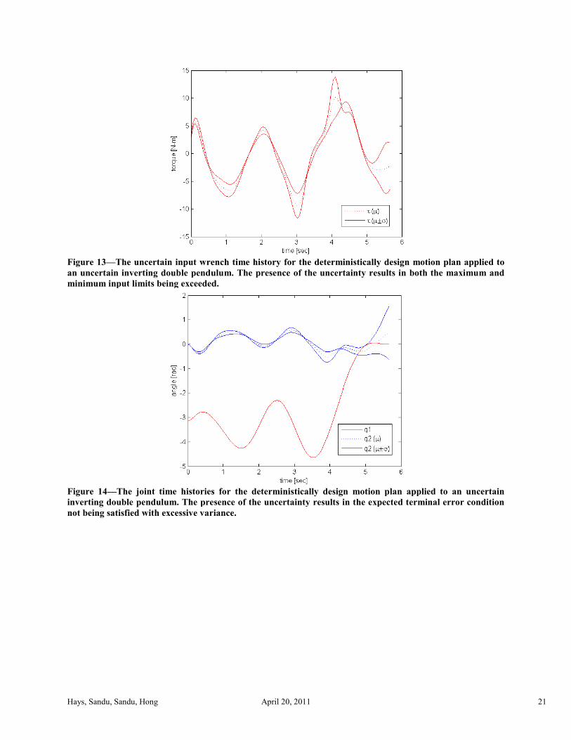
This optimal solution resulted in a ??The value of the new framework is best illustrated by applying the deterministically designed motion profile to an uncertain
system. Figure 13 and Figure 14 show the results of the deterministic motion plan applied to a system with a single uncertainty;
the second link has an uncertain mass with
profile exceeds both the upper and lower bounding constraints of
the target terminal configuration was not satisfied a
Approaching the design with the new framework accounts for the uncertainties up front during the optimal search and results
in a design that satisfies all constraints for all possible systems in the
(45) with constraints defined by (56); where = 4.46 seconds; where the same uncertain second link mass is reused.
configuration time history is illustrated in
histories are displayed. The Euclidean norm of the ÔÕÖ×Ô = 2.61î − 6 6. Figure 16 shows that the input wrench constraints for the entire probability space were satisfied in
a standard deviation sense. Figure 17 show that the specifieÖno = 0.01 6 .
The reduced power of the uncertain design, as compared to the deterministic design, makes sense in that the expected input
wrench values, Q, of the uncertain design (as shown in
in Figure 13). This relationship is also true for
torque and joint rate yields a lower system power.
April 20, 2011
configuration time history for the deterministic inverting double pendulum?? design.
The value of the new framework is best illustrated by applying the deterministically designed motion profile to an uncertain
show the results of the deterministic motion plan applied to a system with a single uncertainty;
with 8 = 1 ² and 8 = 0.5 ² . Figure 13 shows that the resulting input wrench
profile exceeds both the upper and lower bounding constraints of = −10, = 10 ∙ 6. Additionally,
the target terminal configuration was not satisfied and an excessive terminal error variance is experienced.
Approaching the design with the new framework accounts for the uncertainties up front during the optimal search and results
in a design that satisfies all constraints for all possible systems in the probability space. This is accomplished by application of
; where Öno = 0.01 (6 ). This results in a power optimal solution of
where the same uncertain second link mass is reused. The resulting motion plan’s
rated in Figure 15; where the bounding c2 − 2 î", 2 + 2 ì¹&îThe Euclidean norm of the soft expected value terminal configuration constraint was very ac
shows that the input wrench constraints for the entire probability space were satisfied in
show that the specified terminal error variance was also satisfied,
The reduced power of the uncertain design, as compared to the deterministic design, makes sense in that the expected input
of the uncertain design (as shown in Figure 16), are lower than those in the deterministic design (as shown
). This relationship is also true for <Q (although are not illustrated), therefore, the product of the reduced expected
torque and joint rate yields a lower system power.
20
inverting double pendulum.
The value of the new framework is best illustrated by applying the deterministically designed motion profile to an uncertain
show the results of the deterministic motion plan applied to a system with a single uncertainty;
shows that the resulting input wrench
Additionally, Figure 14 shows that
Approaching the design with the new framework accounts for the uncertainties up front during the optimal search and results
probability space. This is accomplished by application of
solution of JË = 310 with
motion plan’s optimal uncertain ì¹&îe configuration time
expected value terminal configuration constraint was very acceptable,
shows that the input wrench constraints for the entire probability space were satisfied in
d terminal error variance was also satisfied, Öno = 0.00321 ≤The reduced power of the uncertain design, as compared to the deterministic design, makes sense in that the expected input
), are lower than those in the deterministic design (as shown
erefore, the product of the reduced expected
Hays, Sandu, Sandu, Hong
Figure 13—The uncertain input wrench
an uncertain inverting double pendulum
minimum input limits being exceeded.
Figure 14—The joint time histories
inverting double pendulum. The presence of the uncertainty results in the expected terminal error condition
not being satisfied with excessive variance.
April 20, 2011
The uncertain input wrench time history for the deterministically design motion plan applied to
uble pendulum. The presence of the uncertainty results in both the maximum and
minimum input limits being exceeded.
ies for the deterministically design motion plan applied to an uncertain
The presence of the uncertainty results in the expected terminal error condition
not being satisfied with excessive variance.
21
motion plan applied to
The presence of the uncertainty results in both the maximum and
motion plan applied to an uncertain
The presence of the uncertainty results in the expected terminal error condition
Hays, Sandu, Sandu, Hong
Figure 15—The power optimal configuration time history
on uncertain hybrid dynamics NLP. This optimal solution resulted in a
Figure 16—The uncertain input wrench
uncertain hybrid dynamics NLP. Both the maximum and minimum input limits were satisfied, in a standard
deviation sense, for all systems within the probability space.
April 20, 2011
configuration time history for the uncertain inverting double pendulum
. This optimal solution resulted in a ? design.
The uncertain input wrench time history resulting from the motion plan generated by
Both the maximum and minimum input limits were satisfied, in a standard
ation sense, for all systems within the probability space.
22
uble pendulum based
y resulting from the motion plan generated by the new
Both the maximum and minimum input limits were satisfied, in a standard
[4] Xiang, Y., Arora, J., and Abdel-Malek, K., 2010, "Physics
Optimization-Based and Other Approaches," Structural and Multidisciplinary Optimization, 42(1), pp. 1
[5] Company, F. M., May 19, 2010, Ford Recruits Virtual Soldier to Boost Quality; Santos Feels the Same Strains That Humans
Do, http://www.prnewswire.com/news-releases/ford
humans-do-94221984.html
[6] Park, J., 2007, Industrial Robotics, Programming, Simulation and Applications, Verlag, Croatia, Optimal Motion Planning f
Manipulator Arms Using Nonlinear Programming.
[7] Chong Jin, O., and Gilbert, E. G., 1996, "Growth Distances: New Measures fo
and Automation, IEEE Transactions on, 12(6), pp. 888
[8] Park, F., Bobrow, J., and Ploen, S., 1995, "A Lie Group Formulation of Robot Dynamics," The International Journal of
Robotics Research, 14(6), pp. 609.
[9] Ploen, S., 1997, "Geometric Algorithms for the Dynamics and Control of Multibody Systems," Ph.D. thesis, University Of
California,
April 20, 2011
ies resulting from the motion plan generated by the new
The resulting terminal error variance satisfies the specification; úÖno =This work has presented a new nonlinear programming based framework for motion planning that treats uncertain
actuated dynamical systems described by ordinary differential equations. The framework allows practitioners
to model sources of uncertainty using the Generalized Polynomial Chaos methodology and to solve the uncertain forward,
-squares collocation method. Subsequently, statistical information
may be included in the NLP’s objective function and constraints to perform optimal motion planning under uncertainty.
studies with uncertain dynamics illustrate how the new framework produces an optimal design that accounts for the
within the associated probability space. This adds robustness to the design of the
expand the new framework to treat constrained dynamical systems described by differential
This work was partially supported by the Automotive Research Center (ARC), Thrust Area 1.
la, S., 2006, "A Clothing Modeling Framework for Uniform and Armor System Design,"
J., Kim, J., Bhatt, R., Rahmatalla, S., Yang, J., Marler, T., Arora, J., and Abdel-Malek, K., 2010,
Based Novel Approach for Human Motion Simulation," Structural and Multidisciplinary
[3] Kim, H., Wang, Q., Rahmatalla, S., Swan, C., Arora, J., Abdel-Malek, K., and Assouline, J., 2008, "Dynamic Motion
d Human Locomotion Using Gradient-Based Optimization," Journal of biomechanical engineering, 130(pp. 031002.
Malek, K., 2010, "Physics-Based Modeling and Simulation of Human Walking: A Review of
her Approaches," Structural and Multidisciplinary Optimization, 42(1), pp. 1-23.
[5] Company, F. M., May 19, 2010, Ford Recruits Virtual Soldier to Boost Quality; Santos Feels the Same Strains That Humans