DAVOODI AND ANDREWS: COMPUTER SIMULATION OF FES STANDING UP IN PARAPLEGIA 153
(a)
(b)
Fig. 2. The rule base of the fuzzy logic controllers modeling the voluntary
arm forcesF
X
(
A)
andF
Y
(
B)
.X ; Y ; V
X , andV
Y are the position andvelocity components of the shoulder joint in the coordinate system shown inFig. 1. X
C
= 0 0 : 1 m (center of the foot support area) and V
S E T
= 0 : 3 5
m/s are used as setpoints for the horizontal position and the vertical velocityof the shoulder joint. The outputs of the controllers are the normalized F
X
and F
Y
that are then linearly scaled to their maximum values. The maximumvalues of F
X
and F
Y
are set at 150 N and total body weight, respectively.N—Negative, P—Positive, Z—Zero, S—Small, M—Medium, L—Large, andV—Very.
by fuzzy logic algorithms with the rules defined heuristically
based on the assumption that these forces primarily provide
balance and help in lifting the body. moves the shoulder
joint toward the center of the foot support area and is a function
of the horizontal position and velocity of the shoulder joint.
maintains a minimum upward speed and prevents downwardmovement of the shoulder joint and is a function of the vertical
position and velocity of the shoulder joint. Unlike and
that could be related to clear objectives and the control
rules could be defined heuristically, it was more difficult to
do the same with and therefore it was not modeled.
Five triangular membership functions were used for each input
variable and seven for each output variable. The membership
functions were all distributed evenly with 50% overlap over
the domain of the variables. The set of rules for the fuzzy
controllers of and are given in Fig. 2.
The equations of motion were derived by applying
D’Alembert–Lagrange principle [27]–[29]. For the planar
model in Fig. 1 to be in general equilibrium the virtual power
must vanish, i.e.
(1)
where is the number of segments, is the mass of
the segment , and are the coordinates of the center of
mass of the segment in an inertial reference frame, is the
generalized coordinate for the segment , and are
the external forces and moments applied to the center of mass
of the segment and is the moment of inertia about an axis
TABLE IMODEL PARAMETERS USED IN THE SIMULATIONS
passing the center of mass of the segment perpendicular to
the sagittal plane.
Application of (1) results in three equations of motion. For
the closed chain system there are two additional constraint
equations
(2)
where is the length of the segment and and are the
vertical and horizontal distances between the wrist and the
ankle joints, respectively. The equations of motion and the
constraint equations must be solved for the angular accelera-
tions, velocities and positions of the joints. In this study, the
shank was fixed to simulate the effect of an ankle foot orthosis
of the floor reaction type [30]. The model parameters for the
simulation experiments are given in Table I.
B. Development of the Learning Algorithms for the FLC-RL
The learning algorithms are combination of a procedure
introduced by Sutton [31], known as the temporal difference
(TD) procedure and the reinforcement learning (RL) procedure[32]. The combined algorithms can address the goal directed
sequential decision making problems, traditionally solved by
dynamic programming [33], [34] but do not require the model
of the environment. The formal convergence proofs have only
been obtained for the finite, stationary markovian decision
process [31], [42], [43]. Although most physical processescannot strictly meet the formal conditions for applying these
techniques, many researchers have been successful in applying
them [35]–[40].
Due to the changes in the body such as muscle fatigue,
the problem posed here is not stationary. Further, the control
actions and states are considered as continuous variables, i.e.,
they can assume infinite number of values. It is our mainobjective however, to evaluate the performance of the RL and
TD in the presence of these violations of the formal conditions.
Fig. 3 illustrates the structure of the learning system. Two
FLC’s represent the knee and hip joint stimulation controllers
8/4/2019 Computer Simulation of Paraplegic Standing 98
154 IEEE TRANSACTIONS ON REHABILITATION ENGINEERING, VOL. 6, NO. 2, JUNE 1998
Fig. 3. Structure of the learning system. FLC’s are used to represent theknee and hip joint stimulation pulsewidth controllers and the value function.Parameter update unit uses the TD error and the structural information of theFLC’s to adjust their parameters. Random search unit (RSU) provides theexploration in the action selection. The detailed description of the learningsystem is given in the text.
and one FLC represents the value function. We call them kneeFLC, hip FLC, and value FLC. The value function
estimates the value of state and is defined as the sum of
the future rewards when starting from state and following a
fixed control policy to the end of the trial. The structure of the
FLC function approximator is shown in Fig. 4. All the FLC’s
receive the partial state information including the knee and hip
joint angular positions (more on this later in discussions)
knee angle, hip angle (3)
The outputs of the knee and hip FLC’s are the stimulation
pulsewidth of the respective joints and . The value
FLC outputs the estimate of the value function . Gaussian
membership functions are used to encode the input variables.
Central values of the membership functions were chosen
for higher concentration in the sensitive regions such as
the terminal phase of standing up and the width values
were chosen for approximately 50% overlap between the
adjacent membership functions as depicted in Fig. 5. The firing
intensities of the fuzzy rules are calculated by applying the
fuzzy multiplication “AND” operator as follows:
AND (4)
where is the rule number, is the firing rate
of the rule and and are the membership values of the
rule’s antecedents. The output of the FLC’s (value FLC forexample) then can be computed as
(5)
where is the parameter vector of the value FLC. Similarly
the parameter vectors for the knee and hip FLC’s are and
, respectively.
The variability and exploration in the action selection poli-
cies (knee and hip joint controllers) are provided by the
random search unit (RSU in Fig. 3) that adds random com-
ponents to and . RSU generates random actions and
Fig. 4. Inference system of a FLC function approximator. For demonstrationpurpose, only two membership functions are used for each input variable. Theactual number of the membership functions are shown in Fig. 5.
Fig. 5. Gaussian membership functions (MF) used to encode the inputvariables. Knee and hip joint angles are represented by 11 and 12 MF’s, re-spectively. The central values of the MF’s are chosen with more concentrationin the dynamically sensitive region around the standing position. The widthof MF’s are chosen for approximately 50% overlap between the neighboringMF’s.
with the mean values of and and a standard deviation
that depends on the value estimate as follows:
(6)
Here, is the standard deviation of the exploration and
determines its maximum value. The standard deviation is
higher when the value estimate is low therefore providing
higher variability in actions to search for higher rewards.
A higher value estimate is a sign that the optimal policy is
approaching when the variability must be lowered to facilitate
the convergence.
The objective of learning (parameter update box in Fig. 3)
is to adjust, in each time step, the parameter vectors of theknee, hip, and value FLC’s. In case of the value function for
example, a general parameter estimation rule [41] can be used
to correct its value
(7)
where is the deviation of from its true value, is the
learning rate, and and are the parameter and feature vectors
from (5), respectively. The parameter update rule for can be
obtained by replacing with TD error,
8/4/2019 Computer Simulation of Paraplegic Standing 98
156 IEEE TRANSACTIONS ON REHABILITATION ENGINEERING, VOL. 6, NO. 2, JUNE 1998
(a)
(b)
Fig. 6. In (a) a unit mass M is shown in a 2-D state space that is 2 m 2 2m in size. Two FLC’s control the accelerations a
x
and a
y
to move, in eachtrial, the unit mass from I (initial state) to G (goal state). The trajectories of M in different stages of learning, when the RL tries to find the quickest pathfrom I to G are shown with the trial numbers next to them. The performanceof the RL in reducing the time spent in each trial is shown in (b).
from the goal state which is the standing position. Coupling
indices represent the effects that each joint’s motion has on the
others and depending on the configuration could be negativeor positive. Although the gravitational forces and the couplingindices in standing up have more complex forms, only constant
values of and are simulated here for simplicity.
When only coupling was implemented, the performance
depended on the sign of the coupling indices. For example, in
ten consecutive simulations, with , the average
number of trials required to reach convergence increased to
178 (range from 60 to 493). Whereas with
the average number of trials required for convergence
decreased to 93 (range from 37 to 150).
The addition of the gravitational term always degraded
the learning rate because it tends to move the mass away
from the goal state. For example, setting the gravity terms
to m/s2 and m/s2 on average
required 189 and 332 trials for convergence, respectively.
D. Computer Implementation
The model of the voluntary arm forces was developed using
MATLAB’s Fuzzy Logic Toolbox (The MathWorks Inc., USA)
and then exported to a C program. The equations of motion,
the three FLC’s of the learning system and the RL algorithms
were all programmed in C. These programs along with the
C code of the voluntary arm forces were implemented in the
DAVOODI AND ANDREWS: COMPUTER SIMULATION OF FES STANDING UP IN PARAPLEGIA 157
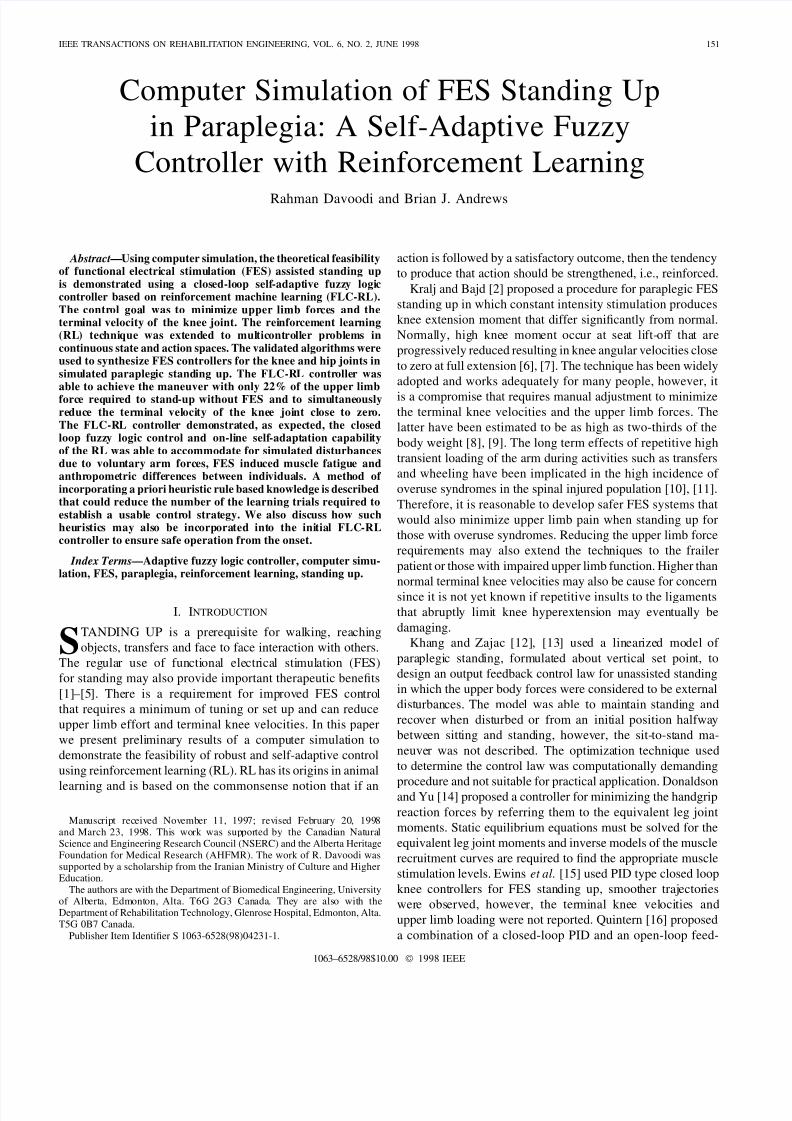
Fig. 7. The performance of the RL when compensating for the inadequatearm forces in standing up. The results are shown for trial 0 (thin), trial10 (medium) and after convergence in trial 29 (thick). Continuous anddashed lines represent the values corresponding to the hip and knee joints,respectively. The stimulation to the knee and hip joint extensors are increased just enough to compensate for the weak arm forces. Note that the stimulationpulsewidth applied to the joints is always positive. The sign of the stimulation
in the figures determines whether it is applied to the extensor or flexor musclesof the joint as explained in the text.
intensity outputs of the FES controllers were set to zero
(the weights of the FLC’s were initially set to zero). The
control actions leading to failure, i.e., not being able to
assume standing position within 4 s were punished by setting
. During standing up, the reward for all other time steps
was zero except for successful trials where the reward wasinversely related to the integral of the arm forces. Therefore,
to maximize its reward, the FLC-RL must learn control
strategies for the knee and hip joints that reduce the arm
forces. The integral of the arm forces was used as a convenient
measure representing, approximately, the energy expended bythe musculature of the upper body. Convergence was assumed
if the last ten trials were all successful and during these ten
trials, the integral of the arm forces did not change by more
than 1% of the maximum value of the integral. The maximum
value of the integral corresponds to the case where no FES
is used to assist standing up, i.e., when maximum arm force
is used.
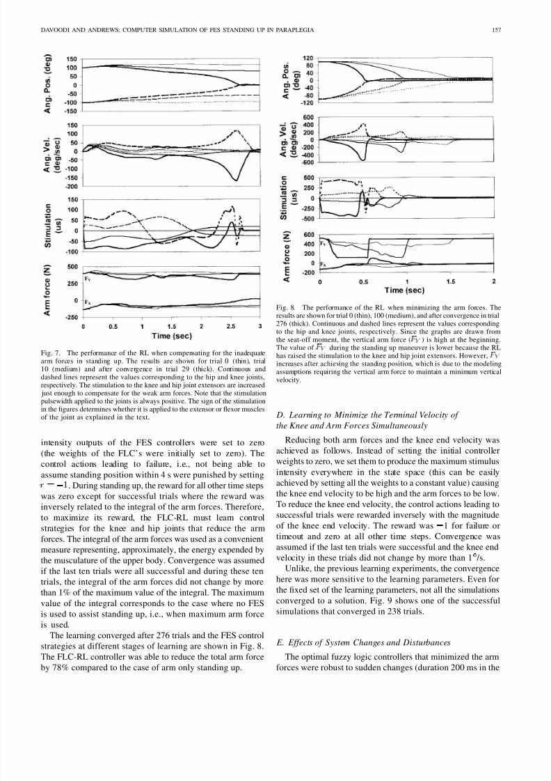
The learning converged after 276 trials and the FES control
strategies at different stages of learning are shown in Fig. 8.
The FLC-RL controller was able to reduce the total arm force
by 78% compared to the case of arm only standing up.
Fig. 8. The performance of the RL when minimizing the arm forces. Theresults are shown for trial 0 (thin), 100 (medium), and after convergence in trial276 (thick). Continuous and dashed lines represent the values correspondingto the hip and knee joints, respectively. Since the graphs are drawn fromthe seat-off moment, the vertical arm force ( F
Y
) is high at the beginning.The value of F
Y
during the standing up maneuver is lower because the RLhas raised the stimulation to the knee and hip joint extensors. However, F
Y
increases after achieving the standing position, which is due to the modelingassumptions requiring the vertical arm force to maintain a minimum verticalvelocity.
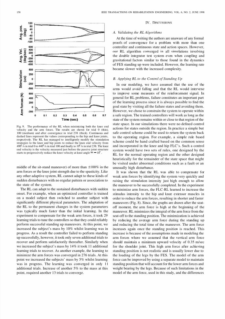
D. Learning to Minimize the Terminal Velocity of
the Knee and Arm Forces Simultaneously
Reducing both arm forces and the knee end velocity was
achieved as follows. Instead of setting the initial controller
weights to zero, we set them to produce the maximum stimulus
intensity everywhere in the state space (this can be easily
achieved by setting all the weights to a constant value) causing
the knee end velocity to be high and the arm forces to be low.
To reduce the knee end velocity, the control actions leading to
successful trials were rewarded inversely with the magnitude
of the knee end velocity. The reward was 1 for failure or
timeout and zero at all other time steps. Convergence was
assumed if the last ten trials were successful and the knee endvelocity in these trials did not change by more than 1 /s.
Unlike, the previous learning experiments, the convergence
here was more sensitive to the learning parameters. Even for
the fixed set of the learning parameters, not all the simulations
converged to a solution. Fig. 9 shows one of the successful
simulations that converged in 238 trials.
E. Effects of System Changes and Disturbances
The optimal fuzzy logic controllers that minimized the arm
forces were robust to sudden changes (duration 200 ms in the
8/4/2019 Computer Simulation of Paraplegic Standing 98
158 IEEE TRANSACTIONS ON REHABILITATION ENGINEERING, VOL. 6, NO. 2, JUNE 1998
Fig. 9. The performance of the RL when minimizing both the knee endvelocity and the arm forces. The results are shown for trial 0 (thin),100 (medium) and after convergence in trial 238 (thick). Continuous anddashed lines represent the values corresponding to the hip and knee joints,respectively. The RL has managed to intelligently modify the stimulationstrategies to the knee and hip joints to reduce the knee end velocity from490 /s in trial 0 to 440 /s in trial 100 and finally to 10 /s in trial 238. The kneeend velocity is the velocity measured just before the passive joint structurestarts to progressively reduce the knee velocity at knee angle = 0 10 .
middle of the sit-stand maneuver) of more than ±100% in thearm forces or the knee joint strength due to the spasticity. Like
any other adaptive system, RL cannot adapt to these kinds of
sudden disturbances with no regular pattern or association to
the state of the system.
The RL can adapt to the sustained disturbances with sudden
onset. For example, when an optimized controller is trained
on a model subject then switched to another subject with
significantly different physical parameters. The adaptation of
the RL to the permanent changes in the system parameters
was typically much faster than the initial learning. In the
experiment to compensate for the weak arm forces, it took 29
learning trials to tune the controllers so that they could reliably
perform successful standing up maneuvers. At this point, weincreased the subject’s mass by 10% whilst learning was in
progress. As a result the controller failed to perform standing
up successfully, however, it took only seven additional trials to
recover and perform satisfactorily thereafter. Similarly when
we increased the subject’s mass by 14% it took 11 additional
learning trials to recover. As another example, the learning to
minimize the arm forces was converged in 276 trials. At this
point we increased the subjects’ mass by 5% whilst learning
was in progress. The learning was converged in only 11
additional trials. Increase of another 5% to the mass at this
point, required another 13 trials to converge.
IV. DISCUSSIONS
A. Validating the RL Algorithms
At the time of writing the authors are unaware of any formal
proofs of convergence for a problem with more than one
controller and continuous state and action spaces. However,
our RL algorithm converged in all simulations involving
the double integrator test system even when coupling andgravitational factors similar to those found in the dynamics
of FES standing up were included. However, the learning rate
became slower with the increased complexity.
B. Applying RL to the Control of Standing Up
In our modeling, we have assumed that the use of the
arms would avoid falling and that the RL would intervene
to improve some measures of the reinforcement signal. In
general for RL problems, failure constitutes an important part
of the learning process since it is always possible to find the
goal state by visiting all the failure states and avoiding them.
However, we chose to constrain the system to operate withina safe region. The trained controllers will work as long as the
state of the system remains within or close to that region of the
state space. In our simulations there were no defined control
actions for states outside the region. In practice a simple but
safe control scheme could be used to return the system back
to the operating region. For example, a simple rule based
scheme could be hand crafted based on the common sense
and incorporated in the knee and hip FLC’s. Such a control
system would have two sets of rules, one designed by the
RL for the normal operating region and the other designed
heuristically for the remainder of the state space that might
be visited under abnormal conditions such as a fault or an
unusually high disturbance.It was shown that the RL was able to compensate for
weak arm forces by identifying the system very quickly and
raising the stimulation intensity just high enough to allow
the maneuver to be successfully completed. In the experiment
to minimize arm forces, the FLC-RL learned to increase the
stimulus intensity to the hip and knee extensor muscles in
order to reduce the arm forces, resulting in shorter and faster
maneuvers (Fig. 8). Since, the graphs are drawn after the seat-
off moment, the arm force is high at the beginning of the
maneuver. RL minimizes the integral of the arm force from the
seat-off to the standing position. The minimization is achieved
by reducing the average arm force during the standing up
and reducing the total time of the maneuver. The arm forceincreases again once the standing position is reached. This
increase is because of the assumptions made in modeling the
arm forces where we assumed that the vertical arm force
should maintain a minimum upward velocity of 0.35 m/sec
for the shoulder joint. This high arm force after achieving
standing position is not realistic and is usually lower due to
the loading of the legs by the FES. The model of the arm
force can be improved by using a separate model to maintain
standing position that will account for the lower arm forces and
weight bearing by the legs. Because of such limitations in the
model of the arm force, used in this study, and the differences
8/4/2019 Computer Simulation of Paraplegic Standing 98
160 IEEE TRANSACTIONS ON REHABILITATION ENGINEERING, VOL. 6, NO. 2, JUNE 1998
The capability to adapt to the changes in the voluntary
control strategy may be one of the strongest aspects of the
RL opening up the possibility for mutual learning. This may
provide a better “cybernetic interface” in which both the
subject and the RL controllers learn to cooperate to perform
the maneuver better since neither the FLC-RL algorithm or the
human require explicit a priori models for learning. Interaction
and reinforcement is all that is needed for the mutual learning
to proceed.
In more conventional closed-loop FES controllers special-
ized sensors are chosen that monitor specific state variables
and must be accurately aligned with the anatomy and precisely
positioned in specific locations, e.g., goniometers across lower
limb joints. This may be inconvenient, particularly if the
sensors are to be surgically implanted. RL however, has no
such requirement and may use any available set of sensory
signals that are sufficiently rich in information about the state
of the system and the reinforcement signal. These could in-
clude sets of miniature artificial sensors located in convenient
external places or implanted [46]–[48] or in combination with
natural sources such as EMG or ENG using electrodes in theperiphery or microelectrodes in the central nervous system.
In such arrangements, the reinforcement signal, such as the
knee velocity if the knee end velocity is to be minimized,
may not be directly available. In such case it must be derived
either intuitively using handcrafted rules or indirectly using
supervised machine learning techniques as described in [47].
The FLC-RL may provide similar flexibility in terms of the
stimulation sites. For example, as an alternative to stimulating
highly differentiated peripheral nerves it may be desirable to
stimulate the spinal cord or the spinal roots and establish
control despite the more complex responses. For example,
stimulating the lumbar anterior sacral roots produces multiple
muscle contractions that affect multiple joints in more than onedegree of freedom [49], [50]. The flexibility in the choice of
inputs and the outputs comes from the fact that the RL process
essentially learns associations between situations and actions.
A further consequence of this feature may offer a measure
of fault tolerance if there is a redundancy in the sensors and
stimulus sites. Should a sensor or stimulus site suddenly or
progressively fail to provide consistent signals or responses
the FLC-RL may progressively learn to discount them from
its control strategy.
To ensure patient safety during the initial training phase
and subsequent use of the RL controller, we envisage an
initial FLC-RL controller based on reliable handcrafted rules,
for example, those commonly used in clinical practice [51],[52]. This “training wheels” possibility is suggested by the
results of the simulation to minimize both the arm forces
and the terminal velocity of the knee joint. Our intuitive
understanding of the system was used to handcraft the initial
controllers so that it was possible to minimize both criteria.
The results of investigating the effects of system changes
suggest an alternative in which an initial controller could be
pretrained by applying the RL algorithm to a dynamical model
approximately scaled to the individual patient. Of course, the
latter would be feasible only if a model was available that also
included the sensors. The latter may not be possible for natural
sensors or when sensor alignment and position is uncertain.
The subsequent learning process which, needs smaller number
of trials to converge, could then continue to fine-tune the
controller without compromising the patient safety.
V. CONCLUSIONS
The classic RL algorithms can be extended to the contin-uous state and action spaces using function approximation
techniques. These algorithms were validated and performed
well in continuous space, multicontroller problems and in the
presence of the simulated complexities normally encountered
in the FES control systems such as dynamic coupling. The
RL was able to learn appropriate strategies to compensate
for the weak arm forces and was able to simultaneously
reduce arm force requirement and the terminal velocity of the
knee joint. The FLC-RL was able to recover from simulated
disturbances approximating those encountered in FES assisted
standing up in paraplegia. It may be possible to include a
priori heuristic rule based knowledge in the learning system
structure, which may accelerate the initial learning rate andprovide safety. Although the method appears to be promising
only the theoretical feasibility has been demonstrated, further
work is required to demonstrate clinical feasibility.
REFERENCES
[1] C. A. Phillips, Functional Electrical Rehabilitation: Technological Restoration After Spinal Cord Injury. New York: Springer-Verlag,1991.
[2] A. Kralj and T. Bajd, Functional Electrical Stimulation: Standing and Walking After Spinal Cord Injury. Boca Raton, FL: CRC Press, 1989.
[3] D. Graupe, Functional Electrical Stimulation for Ambulation by Para- plegics. New York: Krieger, 1994.
[4] B. J. Andrews and G. D. Wheeler, “Functional and therapeutic benefits
of electrical stimulation after spinal injury,” Curr. Opin. Neurol., vol.8, pp. 461–466, 1995.
[5] J. J. Daly, E. B. Marsolais, L. M. Mendell, W. Z. Rymer, A. Stefanovska,J. R. Wolpaw, and C. Kantor, “Therapeutic neural effects of electricalstimulation,” IEEE Trans. Rehab. Eng., vol. 4, pp. 218–230, 1996.
[6] C. A. Doorenbosch, J. Harlaar, M. E. Roebroeck, and G. J. Lankhorst,“Two strategies of transferring from sit-to-stand; The activation of monoarticular and biarticular muscles,” J. Biomechan., vol. 27, pp.1299–1307, 1994.
[7] D. L. Kelly, A. Dainis, and G. K. Wood, “Mechanics and musculardynamics of rising from a seated position,” in Biomechanics, P. V.Komi, Ed. Baltimore, MD: University Park Press, 1976, pp. 127–134.
[8] M. J. Dolan, B. J. Andrews, and J. P. Paul, “Biomechanical evaluation of FES standing up and sitting down in paraplegia,” in IFESS’97, Burnaby,Canada, 1997, pp. 175–176.
[9] R. Kamnik, T. Bajd, and A. Kralj, “Analysis of paraplegics sit-to-standtransfer using functional electrical stimulation and arm support,” in
IFESS’97, Burnaby, Canada, 1997, pp. 161–162.[10] J. S. Bayley, T. P. Cochran, and C. B. Sledge, “The weight-bearing
shoulder: The impingement syndrome in paraplegics,” J. Bone Joint Surg., vol. 69-A, pp. 676–678, 1987.
[11] L. Chisholm, “The angry arm,” Caliper, pp. 13–16, 1997.[12] G. Khang and F. E. Zajac, “Paraplegic standing controlled by functional
neuromuscular stimulation: Part I—Computer model and control-systemdesign,” IEEE Trans. Biomed. Eng., vol. 36, pp. 873–884, 1989.
[13] , “Paraplegic standing controlled by functional neuromuscularstimulation: Part II—Computer simulation studies,” IEEE Trans.
Biomed. Eng., vol. 36, pp. 885–894, 1989.[14] N. d. N. Donaldson and C. H. Yu, “FES standing: Control by handle
reactions of leg muscle stimulation (CHRELMS),” IEEE Trans. Rehab.
Eng., vol. 4, pp. 280–284, 1996.[15] D. J. Ewins, P. N. Taylor, S. E. Crook, R. T. Lipczynski, and I. D. Swain,
“Practical low cost stand/sit system for mid-thoracic paraplegics,” J. Biomed. Eng., vol. 10, pp. 184–188, 1988.
8/4/2019 Computer Simulation of Paraplegic Standing 98
DAVOODI AND ANDREWS: COMPUTER SIMULATION OF FES STANDING UP IN PARAPLEGIA 161
[16] J. Quintern, P. Minwegen, and K. H. Mauritz, “Control mechanisms forrestoring posture and movements in paraplegics,” Prog. Brain Res., vol.80, pp. 489–502, 1989.
[17] K. J. Hunt, M. Munih, and N. d. N. Donaldson, “Feedback control of unsupported standing in paraplegia—Part I: Optimal control approach,”
IEEE Trans. Rehab. Eng., vol. 5, pp. 331–340, 1997.[18] M. Munih, N. d. N. Donaldson, K. J. Hunt, and M. D. B. Fiona,
“Feedback control of unsupported standing in paraplegia—Part II:Experimental results,” IEEE Trans. Rehab. Eng., vol. 5, pp. 341–352,1997.
[19] B. J. Andrews, “Hybrid orthese fur die Fortbevegung von Querschnitts-gelahmten,” Medizinisch-Orthopadische Technik, vol. 110, pp. 84–88,1990.
[20] A. J. Mulder, P. H. Veltink, and H. B. K. Boom, “On/off control in FES-induced standing up. A model study and experiments,” Med. Biologic.
Eng. Comput., vol. 30, pp. 205–212, 1992.[21] A. J. Mulder, P. H. Veltink, H. B. K. Boom, and G. Zilvold, “Low-level
finite state control of knee joint in paraplegic standing,” J. Biomed. Eng., vol. 14, pp. 3–8, 1992.
[22] R. Davoodi and B. J. Andrews, “FES standing up in paraplegia: Acomparative study of fixed parameter controllers,” in Proc. 18th Annu.
Int. Conf. IEEE-EMBS, Amsterdam, The Netherlands, paper no. 784,1996.
[23] D. A. Winter, Biomechanics and Motor Control of Human Movement,2nd ed. New York: Wiley, 1990.
[24] W. K. Durfee and D. J. DiLorenzo, “Linear and nonlinear approachesto control of single joint motion by functional electrical stimulation,” inProc. Amer. Contr. Conf., Green Valley, CA, 1990, pp. 1042–1045.
[25] J. M. Mansour and M. L. Audu, “The passive elastic moment at the kneeand its influence on human gait,” J. Biomechan., vol. 19, pp. 369–373,1986.
[26] D. T. Davy and M. L. Audu, “A dynamic optimization technique forpredicting muscle forces in the swing phase of gait,” J. Biomech., vol.20, pp. 187–201, 1987.
[27] B. Paul, Kinematics and Dynamics of Planar Machinery. EnglewoodCliffs, NJ: Prentice-Hall, 1979.
[28] D. A. Wells, Theory and Problems of Lagrangian Dynamics. NewYork: McGraw-Hill, 1967.
[29] R. E. Roberson and R. Schwertassek, Dynamics of Multibody Systems.Berlin, Germany: Springer-Verlag, 1988.
[30] B. J. Andrews, R. H. Baxendale, R. Barnett, G. F. Phillips, T. Yamazaki,J. P. Paul, and P. A. Freeman, “Hybrid FES orthosis incorporatingclosed loop control and sensory feedback,” J. Biomed. Eng., vol. 10,pp. 189–195, 1988.
[31] R. S. Sutton, “Learning to predict by the methods of temporal differ-
ences,” Machine Learning, pp. 9–44, 1988.[32] A. G. Barto, R. S. Sutton, and C. J. C. H. Watkins, “Learning andsequential decision making,” Unive. Massachusetts, Amherst, COINSTech. Rep. 89–95, 1989.
[33] R. Bellman and R. Kalaba, Dynamic Programming and Modern ControlTheory. New York: Academic, 1965.
[34] S. Ross, Introduction to Stochastic Dynamic Programming. New York:Academic, 1983.
[35] H. R. Beom and H. S. Cho, “Sensor-based navigation for a mobile robotusing fuzzy logic and reinforcement learning,” IEEE Trans. Syst., ManCybern., vol. 25, pp. 464–477, 1995.
[36] V. Gullapalli, “Direct associative reinforcement learning methods fordynamic systems control,” Neurocomput., vol. 9, pp. 271–292, 1995.
[37] W. Ilg and K. Berns, “A learning architecture based on reinforcementlearning for adaptive control of the walking machine LAURON,” Robot.
Autonomous Syst., vol. 15, pp. 321–334, 1995.[38] T. Yamaguchi, M. Masubuchi, K. Fujihara, and M. Yachida, “Realtime
reinforcement learning for a real robot in the real environment,” in Proc. IEEE Int. Conf. Intelligent Robots Syst., 1996, pp. 1321–1328.
[39] M. N. Howell, G. P. Frost, T. J. Gordon, and Q. H. Wu, “Continuousaction reinforcement learning applied to vehicle suspension control,”
Mechatron., vol. 7, pp. 263–276, 1997.[40] A. W. Salatian, K. Y. Yi, and Y. F. Zheng, “Reinforcement learning
for a biped robot to climb sloping surfaces,” J. Robot. Syst., vol. 14,pp. 283–296, 1997.
[41] B. Widrow and S. D. Stearns, Adaptive Signal Processing. EnglewoodCliffs, NJ: Prentice Hall, 1985.
[42] G. A. Rummery and M. Niranjan, “On-line Q-learning using connection-ist systems,” Cambridge University, U.K., CUED/F-INFENG/TR 166,1994.
[43] C. J. H. C. Watkins, Learning From Delayed Rewards. King’s College,Cambridge University, U.K., 1989.
[44] R. S. Sutton and A. G. Barto, An Introduction to Reinforcement Learning.Cambridge, MA: M.I.T. Press, in press.
[45] R. S. Sutton, “Generalization in reinforcement learning: Successful
examples using sparse coarse coding,” Advances in Neural Inform.Processing Syst., vol. 8, pp. 1038–1044, 1996.[46] R. Williamson and B. J. Andrews, “Sensors for FES control,” in Proc.
IFESS’97, Burnaby, B.C., Canada, 1997, pp. 213–215.[47] , “Control of neural prosthesis II: Event detection using ac-
celerometers,” in Proc. RESNA’96, pp. 291–293, 1996.[48] B. J. Andrews and R. Williamson, “Joint motion sensors for FES: The
gyro goniometer,” in Proc. RESNA, 1997.[49] N. d. N. Donaldson, T. A. Perkins, and A. C. M. Worley, “Lumbar
root stimulation for restoring leg function. Methods: Stimulator andmeasurement of muscle actions,” Artificial Organs, vol. 21, pp. 247–249,1997.
[50] D. N. Rushton, T. A. Perkins, N. d. N. Donaldson, D. E. Wood, V. J.Harper, A. M. Tromans, F. M. D. Barr, and D. S. Holder, “LARSI: Howto obtain favorable muscle contractions,” in Proc. IFESS’97, Burnaby,B.C., Canada, 1997, pp. 163–164.
[51] F. Wang, A. Thrasher, and B. J. Andrews, “Control of FES usingunsupervised machine learning,” in Proc. IFESS’97, Burnaby, B.C.,
Canada, 1997, pp. 77–78.[52] F. Wang and B. J. Andrews, “Adaptive fuzzy logic controller for
FES—Computer simulation study,” in Proc. Annu. Int. Conf. IEEE Eng. Med. Biol. Soc., 1994, vol. 16, pp. 406–407.
Rahman Davoodi received the B.S. degree in me-chanical engineering and the M.S. degree in biome-chanical engineering both from Sharif Universityof Technology, Tehran, Iran, in 1988 and 1991,respectively. He is currently pursuing the Ph.D.degree in biomedical engineering at the Universityof Alberta, Edmonton, Alta., Canada.
He has worked as a Lecturer in the University of Air Science and Technology, Iran, as a Research En-
gineer in the aerospace industry, and as a PracticingEngineer in the design of air conditioning systems.
He has used the finite element method in biomechanical problems and heis currently interested in control of FES systems, especially man–machineinteractions, natural motor control and learning, neurofuzzy control, geneticalgorithms, and reinforcement learning.
Brian J. Andrews received degrees in cybernet-ics, control systems, and bioengineering from theUniversities of Reading, Sheffield, and Strathclyde,U.K.
His interests focus on the clinical applicationof control systems technology to assist individualswith spinal injury. He has held clinical and aca-
demic appointments at the University Hospital of Wales, Cardiff, U.K., the University of Strathclyde,Glasgow, Scotland, and the Case Western ReserveUniversity, Cleveland, OH. He is presently Director
of Rehabilitation Technology at the Glenrose Hospital, Edmonton, Alta.,Canada, Professor of Biomedical Engineering at the University of Alberta, andVisiting Professor in the Department of Cybernetics at Reading University.