W OOPY: RETURN TO AlWb ('AWL)

KIRTUliM)AFB, N M E X

COMPUTER SOLUTION OF UNSTEADY NAVIER-STOKES EQUATIONS FOR AN INFINITE HYDRODYNAMIC STEP BEARING

by Henry A, Putre =Pnq*

Lewis Research Center Cleveland, Ohio N A T I O N A L AERONAUTICS A N D SPACE A D M I N I S T R A T I O N W A S H I N G T O N , D. C. APRIL 1970

https://ntrs.nasa.gov/search.jsp?R=19700013956 2019-04-04T22:17:21+00:00Z

1

TECH LIBRARY KAFB, NM

I llllllllllllllHllllllllllllllllllllllllllll 0332554

1. Report No . 2. Government Accession No. 3. Recipient’s Catalog NO. NASA TN D-5682 I

4. T i t l e and Subtitle 5. Report Date COMPUTER SOLUTION O F UNSTEADY NAVIER- April 1970 STOKES EQUATIONS FOR AN INFINITE 6. Performing organization Code

HYDRODYNAMIC S T E P BEARING 7. Authods) 8. Performing Organization Report NO.

Henry A. P u t r e E- 5376

9. Performing organization Name and Address 0 . Work Uni t No.

Lewis Resea rch Center 122-29

National Aeronautics and Space Administration 1. Contract or Grant No.

Cleveland, Ohio 44135 13. Type of Report and Period Covered

12. Sponsoring Agency Name and Address Technical Note National Aeronautics and Space Administration Washington, D. C . 20546

14. Sponsoring Agency Code

15 . Supplementary Notes

Technical F i lm Supplement C-266 available on request .

16. Abstract

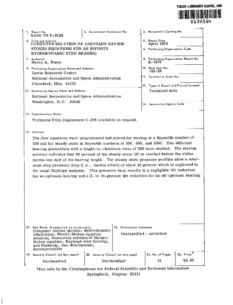
The flow equations were programmed and solved for s t a r tup at a Reynolds number of 100 and for steady-state a t Reynolds numbers of 300, 600, and 1000. Two different bearing geometr ies with a length-to-clearance rat io of 200 were studied. The s t a r tup solution indicates that 99 percent of the steady-state lift is reached before the s l i de r moves one-half of the bearing length. The steady-state p re s su re profiles show a maxi­mum s t e p p r e s s u r e d rop ( i . e . , iner t ia effect) of about 40 percent which is neglected in the usual Rayleigh analysis . This p re s su re drop r e su l t s in a negligible lift reduction f o r a n optimum bearing and a 2- to 14-percent lift reduction f o r a n off-optimum bearing.

17. Key Words ( S u g g e s t e d b y A u t h o r ( s ) ) 18. Distribution Statement Computer motion picture; Hydrodynamiclubrication; Navier-Stokes equation Unclassified - unlimited solution; Numer ica l solution of Navier-Stokes equation; Rayleigh s t e p bearing;and Unsteady , two -dimensional,incompressible *

19. Security Classif . (o f this report) 120. Security Classif.-(of this page) 1 21. No. of Pages I 22. Pr ice

Unclassified 1 Unclassified 31 I $3.00 -

*For sale by the Clearinghouse f o r Fede ra l Scientific and Technical Information Springfield, Virginia 22151

COMPUTER SOLUTION OF UNSTEADY NAVIER-STOKES EQUATIONS

FOR AN INFINITE HYDRODYNAMIC STEP BEARING

by H e n r y A. Putre

Lewis Research Center

SUMMARY

The two-dimensional, unsteady, incompressible, f inite-difference Navier-Stokes equations, together with special inlet and outlet boundary conditions and corner bound­a r y conditions, were programmed and solved for an infinite hydrodynamic step bear­ing. Where possible, the numerical bearing solution was compared to the Rayleigh an­alysis (one-dimensional) solution. The bearing length-to-clearance ratio for these cal­culations was fixed a t 200. Calculations were carried out for Reynolds numbers (Re), based on wall velocity and upstream film thickness, ranging from 100 to 1000.

The unsteady solution with impulse wall startup, which has not been previously pub­lished, was calculated for a Re = 100, optimum geometry (Upstream length/Downstream length = 2.45) bearing. This solution indicates that 99 percent of the steady-state hydro­dynamic lift is achieved in the time the wall moves one-half of the bearing length. In a practical bearing, this amounts to a lift startup time of about 0.0003 second, which is exceedingly small compared to practical bearing startup t imes.

The steady-state solution was calculated for various Reynolds numbers and for an optimum and off-optimum (Upstream length = Downstream length) bearing geometry. In general, these steady-state calculations resolved &hedetailed velocity and pressure field structure in the step region. The important feature of the steady-state numerical solu­tion, which is not accounted for in the Rayleigh analysis, is the pressure drop due to fluid acceleration at the step (i.e. , inertia effect). This pressure drop was found to be as much as 47 percent of the peak pressure at the s tep at a Reynolds number of 1000.

For the optimum geometry bearing, the lift from the numerical solution, including the effect of large s tep pressure drop, was virtually identical to the Rayleigh analysis prediction. For the off-optimum geometry, the s tep pressure drop in the numerical solution caused the lift to range from 2 to 14 percent below the Rayleigh analysis lift for Reynolds numbers from 100 to 1000.

The numerical results are also presented as computer streamline plots and as a computer-generated fluid marker motion picture that is available on request.

I

INTRODUCTION

Recent advances in digital computers and in numerical solution techniques have in­spired the numerical solution of the full Navier-Stokes equations. The earliest numeri­cal solutions published were for steady incompressible flows and simple geometries such as the circular cylinder and the rectangular cavity (refs. 1 and 2). These were followed by the transient incompressible flow solutions , especially the vortex flow development by Fro" and Harlow (ref. 3). Vorticity and s t ream function were generally used as vari­ables , rather than velocity and pressure , for mathematical tractability.

Subsequently, Harlow and Welch (ref. 4) published a transient incompressible solu­tion technique that solves directly for velocity and pressure. An important feature of this technique is that boundary conditions for complicated flows are treated in the prac­tical physical variables , and this technique could also be extended to three-dimensional problems. This transient technique was developed primarily for calculating f ree surface flows, but it can readily be applied to confined flows as well, as was done in a receqt paper by Donovan (ref. 5) for a square cavity.

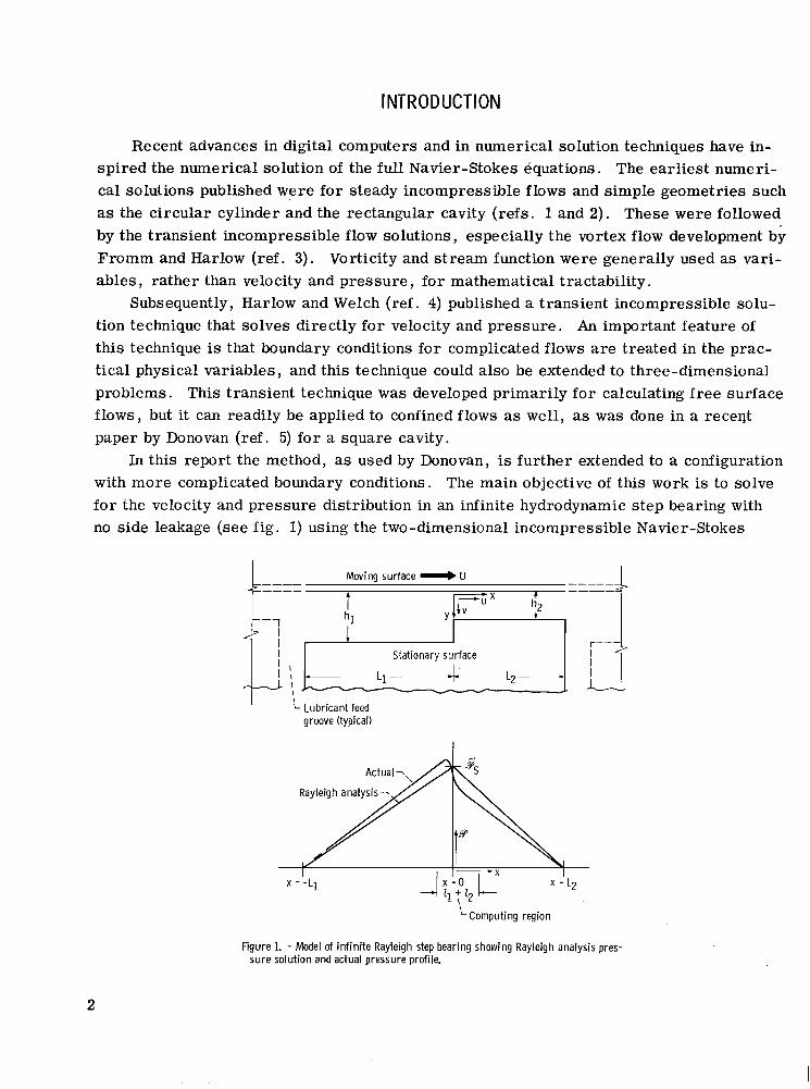
In this report the method, as used by Donovan, is further extended to a configuration with more complicated boundary conditions. The main objective of this work is to solve for the velocity and pressure distribution in an infinite hydrodynamic step bearing with no side leakage (see fig. 1)using the two-dimensional incompressible Navier-Stokes

Moving surface U ____

I Stationary surfaceI

L2­ -I L1-I I

Lubricant feed groove (typical)

x = -L]

'Computing region

Figure L - Model of in f in i te Rayleigh step bearing showing Rayleigh analysis pres­sure solution and actual pressure profile.

2

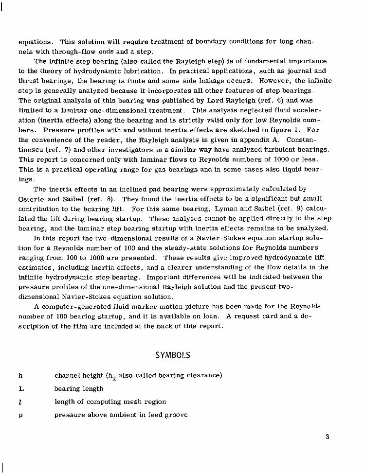
equations. This solution will require treatment of boundary conditions for long chan­nels with through-flow ends and a step.

The infinite step bearing (also called the Rayleigh step) is of fundamental importance to the theory of hydrodynamic lubrication. In practical applications, such as journal and thrust bearings, the bearing is finite and some side leakage occurs. However, the infinite s tep is generally analyzed because it incorporates all other features of step bearings. The original analysis of this bearing was published by Lord Rayleigh (ref. 6) and w a s limited to a laminar one-dimensional treatment. This analysis neglected fluid acceler­ation (inertia effects) along the bearing and is strictly valid only fo r low Reynolds n u ­bers . Pressure profiles with and without inertia effects are sketched in figure l. For the convenience of the reader , the Rayleigh analysis is given in appendix A. Constan­tinescu (ref. 7) and other investigators in a s imilar way have analyzed turbulent bearings. This report is concerned only with laminar flows to Reynolds numbers of 1000 o r less. This is a practical operating range for gas bearings and in some cases also liquid bear­ings.

The inertia effects in an inclined pad bearing were approximately calculated by Osterle and Saibel ( ref . 8). They found the inertia effects to be a significant but small contribution to the bearing lift. For this same bearing, Lyman and Saibel (ref. 9) calcu­lated the lift during bearing startup. These analyses cannot be applied directly to the step bearing, and the laminar s tep bearing startup with inertia effects remains to be analyzed.

In this report the two-dimensional results of a Navier-Stokes equation startup solu­tion for a Reynolds number of 100 and the steady-state solutions for Reynolds numbers ranging from 100 to 1000 a r e presented. These results give improved hydrodynamic lift estimates, including inertia effects, and a clearer understanding of the flow details in the infinite hydrodynamic step bearing. Important differences will be indicated between the pressure profiles of the one-dimensional Rayleigh solution and the present two-dimensional Navier-Stokes equation solution .

A computer-generated fluid marker motion picture has been made for the Reynolds number of 100 bearing startup, and it is available on loan. A request card and a de­scription of the film a r e included at the back of this report .

SYMBOLS

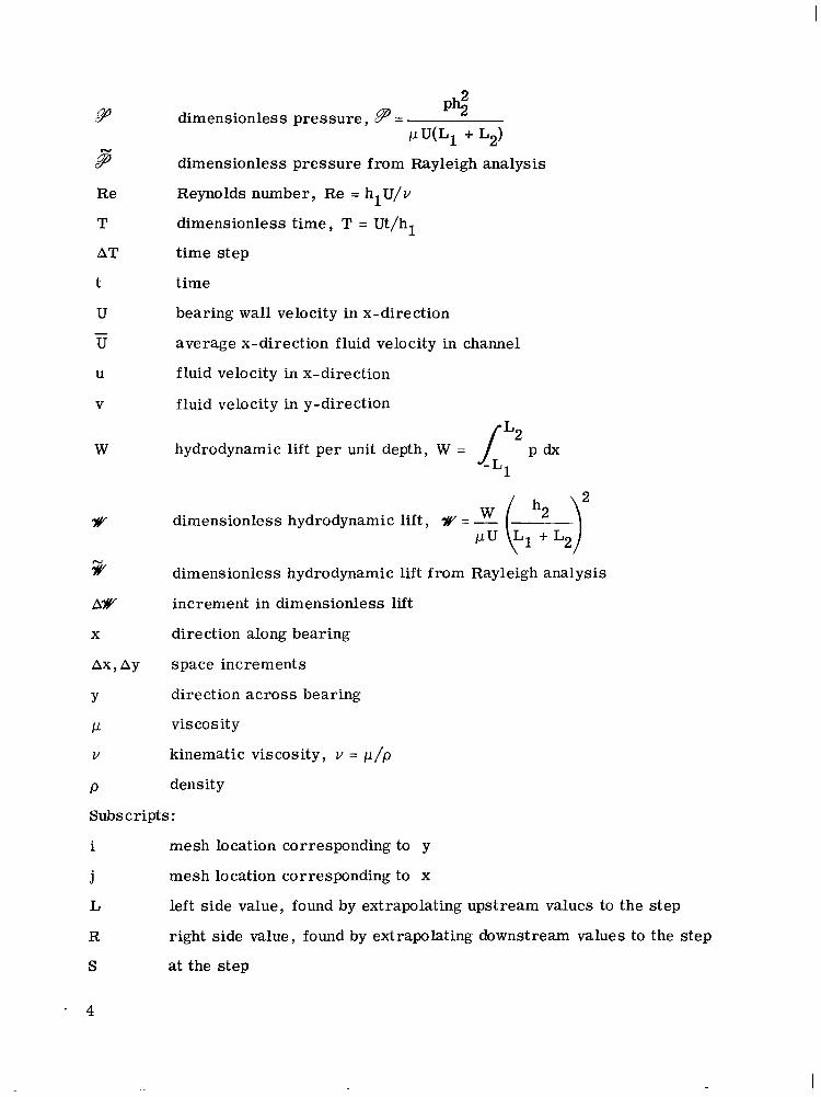
h channel height (hz also called bearing clearance)

L bearing length

t length of computing mesh region

P pressure above ambient in feed groove

3

9 dimensionless -pressure, 9= Ph;

rU.U(L1 + L2) 8 dimensionless pressure from Rayleigh analysis

Re Reynolds number, Re = hlU/v

T dimensionless t ime, T = Ut/hl

AT time step

t time

U bearing wall velocity in x-direction -U average x-direction fluid velocity in channel

U fluid velocity in x-direction

V fluid velocity in y-direction

W hydrodynamic lift per unit depth, W =

% dimensionless hydrodynamic lift from Rayleigh analysis

AW increment in dimensionless lift

X direction along bearing

Ax, Ay space increments

Y direction across bearing

rU. vis cosity

V kinematic viscosity, v = p / p

P density

Subscripts:

i mesh location corresponding to y

j mesh location corresponding to x

L left side value, found by extrapolating upstream values to the step

right side value, found by extrapolating downstream values to the stepR

S at the step

1

2

upstream of s tep

downstream of s tep

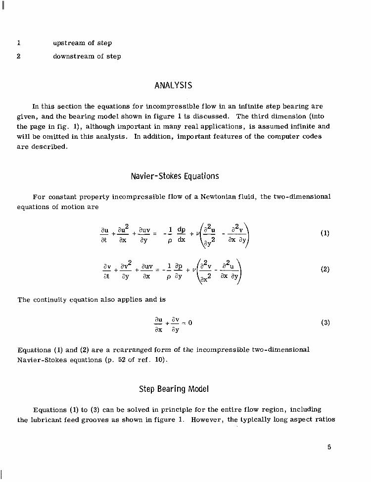
ANALY S I S

In this section the equations for incompressible flow in an infinite step bearing are given, and the bearing model shown in figure 1is discussed. The third dimension (into the page in fig. 1), although important in many real applications, is assumed infinite and wil l be omitted in this analysis. In addition, important features of the computer codes are described.

Navier-Stokes Equat ions

For constant property incompressible flow of a Newtonian fluid, the two-dimensional equations of motion a r e

The continuity equation also applies and is

Equations (1)and (2) are a rearranged form of the incompressible two-dimensional Navier-Stokes equations (p. 52 of ref. 10).

Step Bearing Model

Equations (1)to (3) can be solved in principle for the entire flow region, including the lubricant feed grooves as shown in figure 1. However, the typically long aspect ratios

5

Ll/hl and L2/h2 indicate that the flow over most of the bearing length outside the s tep vicinity will be one-dimensional. For this reason, and in order to conserve computer storage, the Navier-Stokes equation computing region extends over only a portion of the bearing length 1 + z 2 in the vicinity of the s tep (see fig. 1). The remainder of the flow outside the computing region is treated as one-dimensional. In agreement with standard practice, the bearing end pressures a r e assumed equal to the ambient feed groove pres­sure . (A more precise evaluation of the bearing end pressures , which is of secondary importance, would require a more extensive analysis including flow in the feed grooves. )

The step bearing is therefore divided into three regions:

One-dimensional unsteady flow with p(-L1) = 0 for

Two-dimensional unsteady flow , Navier-Stokes equation solution for

One-dimensional unsteady flow with p(+L2) = 0 f o r

The technique of choosing the computing lengths I and is presented in a later se ction.

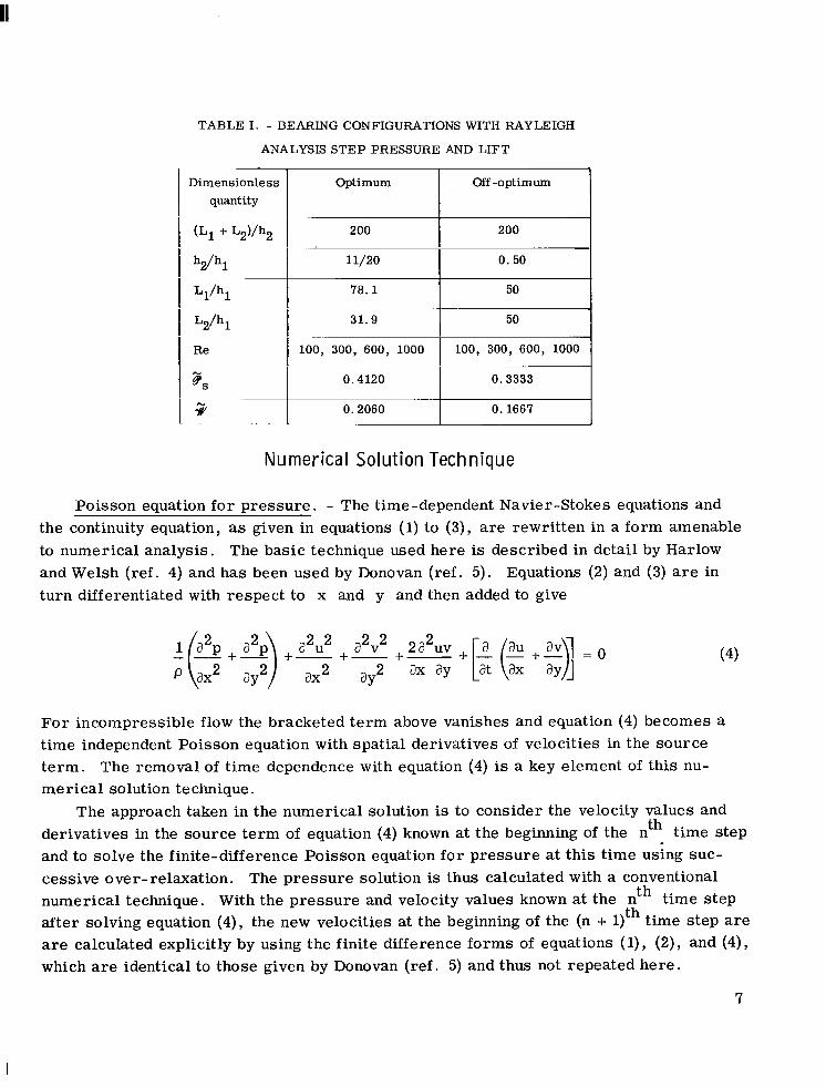
The various step bearing configurations that were analyzed a r e now discussed. The configuration is specified completely by the four dimensionless quantities Re, (L1 + L2)/h2, hl/h2, and L1/L2. The Reynolds number has values ranging from 100 to 1000. The aspect ratio, which in practice is fixed by fabrication tolerances for clear­ance and space availability for length, is fixed at (L1 + L2)/h2 = 200 (typical values a r e h2 = 0.01 cm and L1 + L2 = 2 cm). Two bearing geometries a r e analyzed. One, referred to as the optimum bearing, has proportions very close to the optimum Rayleigh bearing (see appendix A) with hl/h2 determined by the numerical mesh s ize and LI/L2 = (hl/h2)3/2 according to equation (A6). The other is a typical off-optimum geometry. These bearing configurations a r e summarized in table I . The Rayleigh analysis step pressure and lift calculated from equations (A4) and (A5) a r e also shown.

6

TABLE I . - BEARING CONFIGURATIONS WITH RAYLEIGH

ANALYSIS STEP PRESSURE AND LIFT

Dimensionless Optimum Off-optimum quantity

200 I 200

11/20 I 0.50

78.1 I 50

31.9 I 50

0.4120 0.3333

0.2060 I 0.1667

Numerical Solution Technique

Poisson equation for pressure. - The time-dependent Navier-Stokes equations and the continuity equation, as given in equations (1)to (3), a r e rewritten in a form amenable to numerical analysis. The basic technique used here is described in detail by Harlow and Welsh (ref. 4)and has been used by Donovan (ref. 5). Equations (2) and (3) a r e in turn differentiated with respect to x and y and then added to give

For incompressible flow the bracketed te rm above vanishes and equation (4)becomes a time independent Poisson equation with spatial derivatives of velocities in the source te rm. The removal of time dependence with equation (4)is a key element of this nu­merical solution technique.

The approach taken in the numerical solution is to consider the velocity values and derivatives in the source te rm of equation (4)known at the beginning of the nth time step and to solve the finite-difference Poisson equation for pressure at this time using suc­cessive over-relaxation. The pressure solution is thus calculated with a conventional numerical technique. With the pressure and velocity values known at the nth time step after solving equation (4),the new velocities at the beginning of the (n + l)thtime step are are calculated explicitly by using the finite difference forms of equations (1), (2), and (4), which are identical to those given by Donovan (ref. 5) and thus not repeated here .

7

Ax j-

AY

i (a) Placement of field variables.

(b) Typical computing mesh layout.

Figure 2. - Typical field variable placement and computing mesh layou t

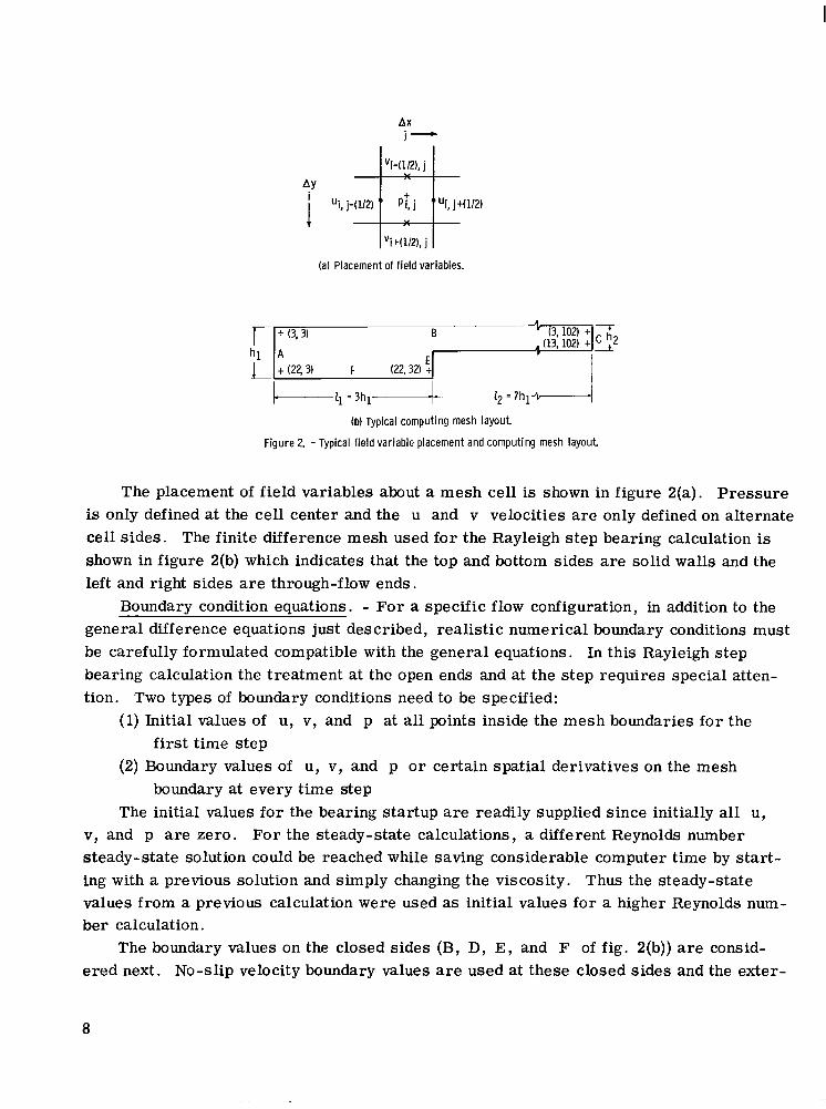
The placement of field variables about a mesh cell is shown in figure 2(a). Pressure is only defined at the cell center and the u and v velocities a r e only defined on alternate cell sides. The finite difference mesh used f o r the Rayleigh s tep bearing calculation is shown in figure 2(b) which indicates that the top and bottom sides a r e solid walls and the left and right sides are through-flow ends.

Boundary condition equations. - For a specific flow configuration, in addition to the general difference equations just described, realistic numerical boundary conditions must be carefully formulated compatible with the general equations. In this Rayleigh step bearing calculation the treatment at the open ends and at the step requires special atten­tion. Two types of boundary conditions need to be specified:

(1)Initial values of u, v, and p at all points inside the mesh boundaries for the first time step

(2) Boundary values of u, v, and p o r certain spatial derivatives on the mesh boundary at every time step

The initial values for the bearing startup are readily supplied since initially all u, v, and p a r e zero. For the steady-state calculations, a different Reynolds number steady-state solution could be reached while saving considerable computer time by s tar t ­ing with a previous solution and simply changing the viscosity. Thus the steady-state values from a previous calculation were used as initial values for a higher Reynolds num­ber calculation.

The boundary values on the closed sides (B, D, E , and F of fig. 2(b)) a r e consid­ered next. No-slip velocity boundary values a r e used at these closed sides and the exter­

8

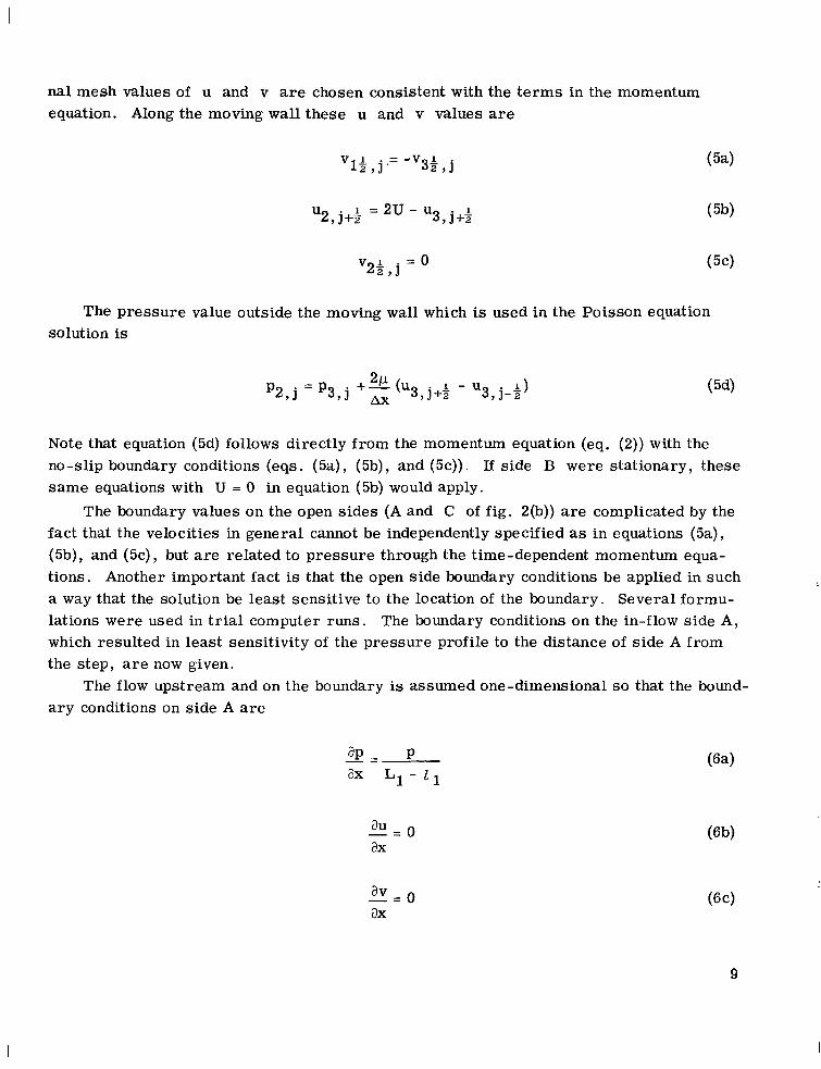
nal mesh values of u and v are chosen consistent with equation. Along the moving wall these u and v values

v 1 . = - v 11 2 , J ' 32 , j

u2,j++ = 2u - u3, j++

the t e rms in the momentum are

(5 4

(5b)

( 5 4

The pressure value outside the moving wall which is used in the Poisson equation solution is

Note that equation (5d) follows directly from the momentum equation (eq. (2)) with the no-slip boundary conditions (eqs. (5a), (5b), and (5c)). Lf side B were stationary, these same equations with U = 0 in equation (5b) would apply.

The boundary values on the open sides (A and C of fig. 2(b)) a r e complicated by the fact that the velocities in general cannot be independently specified as in equations (5a), (5b), and (5c), but a r e related to pressure through the time-dependent momentum equa­tions. Another important fact is that the open side boundary conditions be applied in such a way that the solution be least sensitive to the location of the boundary. Several formu­lations were used in t r ia l computer runs. The boundary conditions on the in-flow side A, which resulted in least sensitivity of the pressure profile to the distance of side A from the step, a r e now given.

The flow upstream and on the boundary is assumed one-dimensional so that the bound­a r y conditions on side A a r e

au- = o ax

av- = o ax

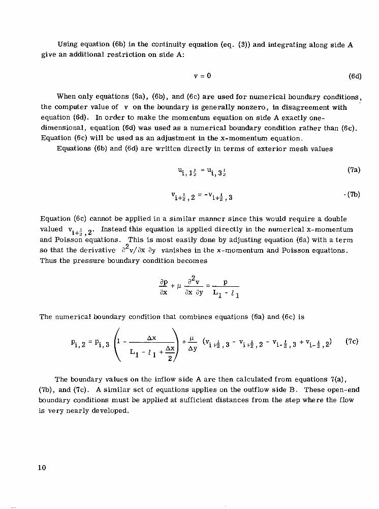
Using equation (6b) in the continuity equation (eq. (3)) and integrating along side A give an additional restriction on side A:

When only equations (sa), (6b), and (6c) are used fo r numerical boundary conditions, the computer value of v on the boundary is generally nonzero, in disagreement with equation (6d). In order to make the momentum equation on side A exactly one-dimensional, equation (6d) was used as a numerical boundary condition rather than (6c). Equation (6c) will be used as an adjustment in the x-momentum equation.

Equations (6b) and (6d) are written directly in t e rms of exterior mesh values

Equation (6c) cannot be applied in a similar manner since this would require a double Ivalued v.l + Z , 2 ' Instead this equation is applied directly in the numerical x-momentum

and Poisson equations. This is most easily done by adjusting equation (sa) with a te rm so that the derivative a2v/ax ay vanishes in the x-momentum and Poisson equations. Thus the pressure boundary condition becomes

2 - + p - - a v - PaP ax ax ay L~ - z 1

The numerical boundary condition that combines equations (sa) and (6c) is

The boundary values on the inflow side A a r e then calculated from equations 7(a), (7b), and (7c). A similar se t of equations applies on the outflow side B. These open-end boundary conditions must be applied at sufficient distances from the step where the flow is very nearly developed.

10

Corner Ambiguities

At the 90' corners (as, e .g . , between sides A and B o r E and F in fig. 2(b)), the velocity and pressure boundary values can be applied in a straightforward manner. The boundary conditions at the 270' corner (between sides D and E) , however, are more dif­ficult to apply because some points on and outside the boundary are required to have more than one value. This situation was remedied by rewriting the finite-difference x and y momentum equations and the Poisson equation at the three cells that meet in this corner so that the boundary values are used directly in the equations.

Computer Codes

Numerical solution code. - The finite-difference equations and the boundary value equations were programmed in FORTRAN IV f o r calculations on an IBM 7094 computer. In the computer code the values of U, hl , and p are arbitrari ly se t at one. This code includes two accuracy checks which should be satisfied a t each time step. The first, a convergence tes t , requires that the Poisson equation iterations give local pressure val­ues that vary l e s s than 10-3/Re within successive pressure iterations. The second, a continuity and mathematical consistency check, requires that the quantity (au/ax) + (av/ay) for each cell be small , l ess than about 2X10-2/Re, if the incompressible difference equa­tions have been correctly applied. Time step values ranging from AT = 0.02 to 0.05 were used in calculations. A typical mesh consisted of 100 mesh intervals of Ax = 0.10 by 20 mesh intervals of Ay = 0.05. With a 100 by 20 mesh s ize and a time step of AT = 0.05, about 90 minutes a r e required on the IBM 7094 to carry the calculations out to near steady s ta te , o r T = 46 at Re = 100. Listed output at specified time intervals f rom the code a r e u, v, p, continuity and pressure convergence checks at each cell, and integrated pressure along the moving wall .

Visual -

display computer codes. - A second code was written for converting the large ~~

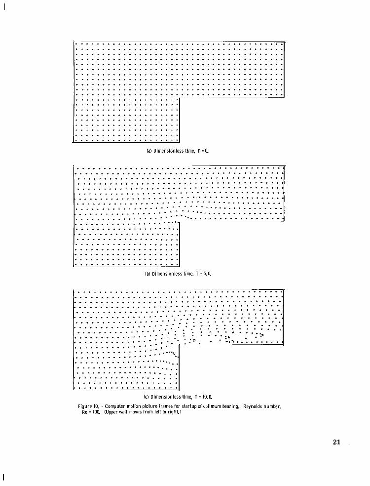
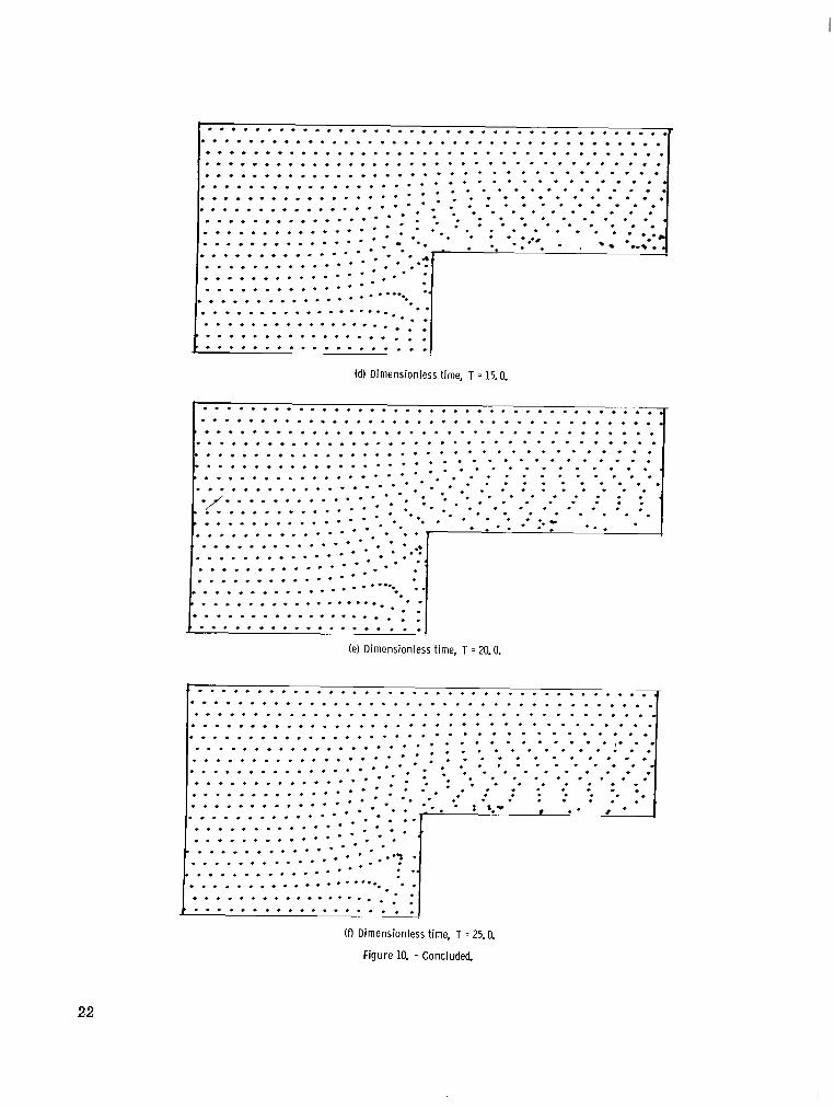
amount of information from the numerical solution code into a ser ies of animated pictures which show the location of fluid markers as they a r e moved in time and space by the ve­locity field. The technique which results in a computed motion picture of the flow has been used by Harlow and Welsh (ref. 4) and also by Donovan (ref. 5). A motion picture was made f o r the Re = 100 startup case. Several f rames f rom this movie a r e shown in figure 10 and will be discussed la ter (p. 19).

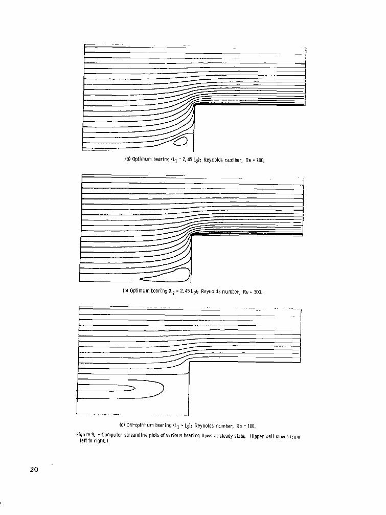
A third code , which is basically s imilar to the movie code , was written to provide a streamline picture of the flow field at any time interval. This code dramatically shows in a single f rame the very fine details of the flow field. Streamline pictures at very near steady state are shown for several cases in figure 9 (to be discussed la ter , p. 19). Of

11

I

particular note here is the fact that these pictures illustrate the flow pattern even in a region where velocities a r e very small , such as ahead of the step.

RESULTS AND DISCUSSION

Numerical Results

The results of the numerical calculations are presented in several par ts . F i r s t , a general accuracy check of this computer code is described. Next, the flow startup solution is discussed for the Re = 100 optimum bearing. This is followed by a discussion of the steady-state solution for Reynolds numbers ranging from 100 to 1000 for the optimum and off -optimum step bearings. Important differences between the numerical solution and the Rayleigh step solution, especially concerning pressure and hydrodynamic lift, a r e em­phasized.

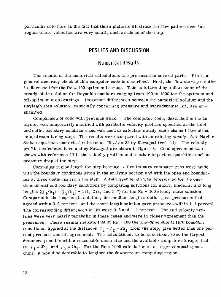
Comparison of code with previous work. - The computer code, described in the an­alysis, was temporarily modified with parabolic velocity profiles specified as the inlet and outlet boundary conditions and w a s used to calculate steady-state channel flow about an upstream facing step. The results were compared with an existing steady-state Navier-Stokes equations numerical solution at Uhl/v = 32 by Kawaguti (ref. 11). The velocity profiles calculated here and by Kawaguti a r e shown in figure 3. Good agreement was shown with reference 11 in the velocity profiles and in other important quantities such as pressure drop at the step.

Computing region length for step bearing. - Preliminary computer runs were made with the boundary conditions given in the analysis section and with the open end boundar­ies at three distances from the step. A sufficient length was determined for the one-dimensional end boundary conditions by comparing solutions for short , medium, and long lengths ((Il/hl) + (I 2/hl) = 1+1, 2+2, and 3+7) for the Re = 100 steady-state solution. Compared to the long length solution, the medium length solution gave pressures that agreed within 0 .6 percent, and the short length solution gave pressures within 1.1percent. The corresponding differences in lift were 0 . 5 and 1.1percent. The end velocity pro­files were very nearly parabolic in these cases and were in closer agreement than the pressures . These results indicate that at Re = 100 the one-dimensional flow boundary conditions, applied at the distances I = z 2 = 2hl from the step, give better than one per­cent pressure and lift agreement. The calculations, to be described, used the largest distances possible with a reasonable mesh size and the available computer storage, that is, 1 = 3hl and z 2 = 7hl. Fo r the Re = 1000 calculation on a larger c6mputing ma­chine, it would be desirable to lengthen the downstream computing region.

12

c

r

W

W

0

3.0

2.5

solut ion

‘2 =I

z- 2.0 c r ref. 11 m U

010-

1.5 c.­-8 > UN .-­m 1.0E z

. 5

0

Figure 3. - Steady-state velocity profiles for channel flow wi th step calculat ion check for Re = (Uhlv) = 32.

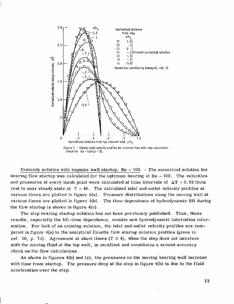
Unsteady solution with impulse wall startup, Re = 100. - The numerical solution for bearing flow startup was calculated for the optimum bearing at Re = 100. The velocities and pressures a t every mesh point were calculated at time intervals of A T = 0.05 from res t to near steady s ta te a t T = 46. The calculated inlet and outlet velocity profiles at various times are plotted in figure 4(a). Pressure distributions along the moving wall at various t imes are plotted in figure 4(b). The time dependence of hydrodynamic lift during the flow startup is shown in figure 4(c).

The step bearing startup solution has not been previously published. Thus, these results , especially the lift-time dependence, contain new hydrodynamic lubrication infor­mation. Fo r lack of an existing solution, the inlet and outlet velocity profiles are com­pared in figure 4(a) to the analytical Couette flow startup solution profiles (given in ref. 10, p. 74). Agreement at short t imes (T 4 4), when the step does not interfere with the moving fluid at the top wall, is excellent and constitutes a second accuracy check on the flow calculations.

As shown in figures 4(b) and (c), the pressures on the moving bearing wall increase with time from startup. The pressure drop at the step in figure 4(b) is due to the fluid acceleration over the step.

13

VI

c

L

VI

Normalized time, T

Couette flow startup solut ion from Schl icht ing (ref. 10)

. 2 . 4 . 6 . 8 1.0 0 . 2 . 4 .55 Nor malized distance from moving bearing wall, ylhl

(a-1) Upstream of step, x/hl = -3.0. (a-2) Downstream of step, x l h l = t7.0.

(a) Velocity profiles at various times f rom bearing startup. -1.6

-. 4 - Normalized t ime 1.4- from startup,

7 -1. 2

N -. 3 .a n3 z- 1.0­

a-L 33 VI

VIVI a

CL2 .8­n VI

1 . 2 _ V I a--a c 0c ._0._ c . 6 -

VIa E .-E ._ n n

. 4 ­.1 4

. 2 ­

0 - 0 I I l l I I I I -3 -2 -1 0 1 2 3 4 5 6 7

(b) Pressure variat ion along moving wall du r ing bearing startup.

Figure 4. - Velocities, pressures, and l i f t calculated f rom impulse wall startup to steady state. Reynolds number, 100; L2 = 2.45 L1; optimum bearing configuration.

14

In al

c

* -.-0

c* E._ a

Time from impulse wall startup, T

(c) Variat ion of hydrodynamic l i f t w i th t ime from bearing startup.

Figure 4. - Concluded.

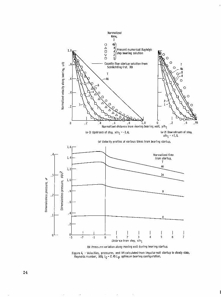
The consequences of this step pressure drop a r e discussed in the next section. The lift variation with time shows that 99 percent of the steady-state value is reached in the di­mensionless time T = 46. In practical t e rms , this means that, with a moving wall speed of say 30 meters per second and a channel height hl of 0.02 centimeter, the bearing has developed 99 percent of its lift in a time of 0.0003 second. This flow relaxation t ime is very small when compared to practical wall startup t imes which are of the order of sec­onds. This indicates that the common practice, for unsteady wall speeds of superim­posing steady-state lift solutions during any bearing transients is valid.

Another interesting aspect of the lift-time curve is the sharp lift increase in fig­ure 4(c) at about T = 2.5. This time delay to lift increase can be accounted for by using figure 4(a) as the time required for the upstream velocity to become nonzero at y = h2. A s imilar time delay was noted in reference 9 for the inclined pad bearing startup.

Steady-state solution for various Reynolds numbers. - The same computer code that was used for the previous startup calculation was also used for steady-state calculations at various Reynolds numbers. The calculations for the optimum geometry a r e presented first, followed by the off-optimum geometry calculations.

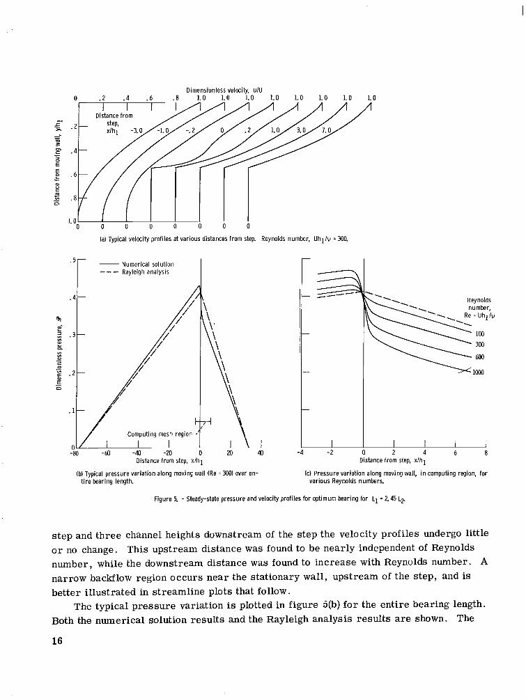
Steady-state velocity and pressure profiles were calculated for the L1 = 2.45 L2 geometry at the Reynolds numbers of 100, 300, 600, and 1000. The calculations were carr ied out to AW/AT < At this cutoff the velocity profiles on sides A and C a r e very nearly parabolic. Typical steady-state velocity profiles and the pressure along the moving wall a r e plotted in figures 5(a) and (b) for a Reynolds number of 300. The velocity profile plot in figure 5(a) indicates that beyond about one channel height upstream of the

15

---

Dimensionless velocity, u/U 0 . 2 .4 .6 .8 1.0 1.0 1.0 1.0 1.0 1.0 1.0 1.0

0 0 0 0 0

(a) Typical velocity profiles at various distances from step. Reynolds number, U h l l u = 300.

--Numerical solution

Rayleigh analysis

I 'I 40 -2 U 2 4 6 8

Distance from step, x l h l Distance from step, x l h l

(b) Typical pressure variation along moving wall (Re = 300)over en- (c) Pressure variation along moving wall, i n computing region, for t i re bearing length. various Reynolds numbers.

Figure 5. - Steady-state pressure and velocity profiles for optimum bearing for L1 = 2.45 L2

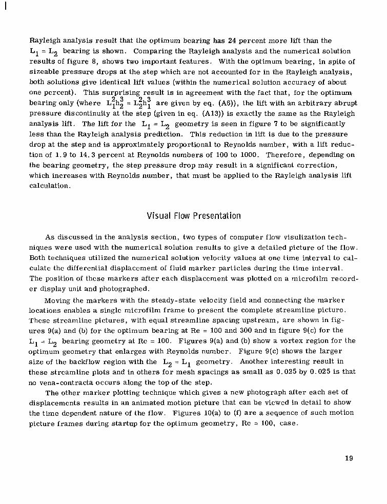
step and three channel heights downstream of the step the velocity profiles undergo little o r no change. This upstream distance was found to be nearly independent of Reynolds number, while the downstream distance was found to increase with Reynolds number. A narrow backflow region occurs near the stationary wall, upstream of the step, and is better illustrated in streamline plots that follow.

The typical pressure variation is plotted in figure S(b) for the entire bearing length. Both the numerical solution results and the Rayleigh analysis results are shown. The

16

0

numerical solution pressure drop in the vicinity of the s tep should be noted. This pres­sure drop is mainly due to fluid acceleration near the step. The net result of this s tep pressure drop is that in the upstream region the pressures and hydrodynamic lift are greater than predicted by the Rayleigh analysis. The opposite is t rue in the downstream region.

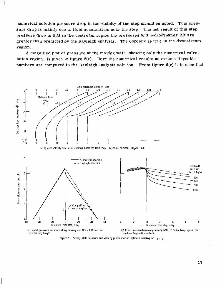
A magnified plot of pressure at the moving wall , showing only the numerical calcu­lation region, is given in figure 5(c). Here the numerical results at various Reynolds numbers are compared to the Rayleigh analysis solution. From figure 5(c) it is seen that

- 2

. 6 c

u

mc.= . a n

LO 0 0 0 0 0 0 0 0 0

(a) Typical velocity profiles at various distances from step. Reynolds number, U h l l v = 300.

_ Numerical Solution Rayleigh analysis

Reynolds -e@- number,

I I I u -4 -2 0 2 4 6 8

Distance from step, x l h l Distance from step, x l h l

(bl Typical pressure variation along moving wall (Re = 3M1) over en- (c) Pressure variation along moving wall, i n computing region, for t i re bearing length. various Reynolds numbers.

Figure 6 - Steady-state pressure and velocity profiles for off-optimum bearing for L1 = Lp

17

Re

the s tep pressure drop effect increases with Reynolds number. The off-optimum geometry (L1 = Lz)calculations were carr ied out for Reynolds num­

bers of 100, 300, 600, and 1000. Typical velocity profiles and pressure profiles are plotted in figure 6. A comparison of the velocity profiles in figures 5(a) and 6(a) shows that the L1 = La geometry has a la rger backflow region upstream of the step that oc­cupies about one-fourth of the channel height. This larger backflow region is also pre­dicted by the Rayleigh analysis. The moving wall p ressures in the s tep region, shown in figure 6(b), have approximately the same variation as those fo r the optimum geometry in figure 5(b).

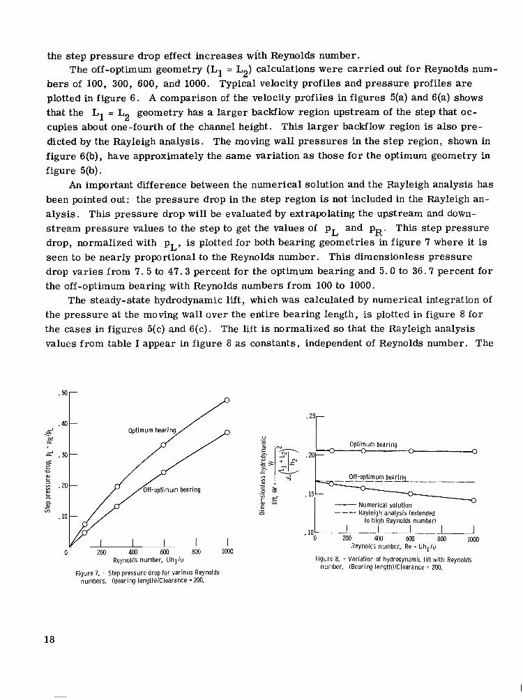
An important difference between the numerical solution and the Rayleigh analysis has been pointed out: the pressure drop in the step region is not included in the Rayleigh an­alysis. This pressure drop will be evaluated by extrapolating the upstream and down­s t ream pressure values to the step to get the values of pL and pR. This step pressure drop, normalized with pL, is plotted for both bearing geometries in figure 7 where it is seen to be nearly proportional to the Reynolds number. This dimensionless pressure drop varies from 7 . 5 to 47.3 percent for the optimum bearing and 5.0 to 36.7 percent fo r the off -optimum bearing with Reynolds numbers f rom 100 to 1000.

The steady-state hydrodynamic lift , which was calculated by numerical integration of the pressure at the moving wall over the entire bearing length, is plotted in figure 8 for the cases in figures 5(c) and 6(c). The lift is normalized so that the Rayleigh analysis values from table I appear in figure 8 as constants, independent of Reynolds number. The

Optimum bearing .20

Off-opti mum bearing __________ .15­

n

Numerical solution 71

Rayleigh analysis (extended to high Reynolds number)

-__.I -I-II 200Reynolds4001001,number, 600= U h l l v800 1000

0 200 400 600 800 Reynolds number, U h l l u Figure 8. - Variation of hydrodynamic l i f t with Reynolds

number. (Bearing IengthllClearance = 2M).Figure 7. - Step pressure drop for various Reynolds

numbers. (Bearing 1ength)lClearance = 200.

18

Rayleigh analysis result that the optimum bearing has 24 percent more lift than the L1 = L2 bearing is shown. Comparing the Rayleigh analysis and the numerical solution resul ts of figure 8, shows two important features. With the optimum bearing, in spite of sizeable pressure drops at the step which a r e not accounted for in the Rayleigh analysis, both solutions give identical lift values (within the numerical solution accuracy of about one percent). This surprising result is in agreement with the fact that, for the optimum.

2 3bearing only (where L:hi = L2hl are given by eq. (A6)), the lift with an arbi t rary abrupt pressure discontinuity at the s tep (given in eq. (A13)) is exactly the same as the Rayleigh analysis lift. The lift for the L1 = La geometry is seen in figure 7 to be significantly l e s s than the Rayleigh analysis prediction. This reduction in lift is due to the pressure drop at the step and is approximately proportional to Reynolds number, with a lift reduc­tion of 1.9 to 14.3 percent at Reynolds numbers of 100 to 1000. Therefore, depending on the bearing geometry, the s tep pressure drop may result in a significant correction, which increases with Reynolds number, that must be applied to the Rayleigh analysis lift calculation.

Vis ua I FIow Presentat ion

As discussed in the analysis section, two types of computer flow visulization tech­niques were used with the numerical solution results to give a detailed picture of the flow. Both techniques utilized the numerical solution velocity values at one time interval to cal­culate the differential displacement of fluid marker particles during the time interval. The position of these markers after each displacement was plotted on a microfilm record­e r display unit and photographed.

Moving the markers with the steady-state velocity field and connecting the marker locations enables a single microfilm frame to present the complete streamline picture. These streamline pictures, with equal streamline spacing upstream, a r e shown in fig­ures 9(a) and (b) for the optimum bearing at Re = 100 and 300 and in figure 9(c) for the L1 = L2 bearing geometry at Re = 100. Figures 9(a) and (b) show a vortex region for the optimum geometry that enlarges with Reynolds number. Figure 9(c) shows the larger s ize of the backflow region with the L2 = L1 geometry. Another interesting result in these streamline plots and in others for mesh spacings as small as 0.025 by 0.025 is that no vena-contracta occurs along the top of the step.

The other marker plotting technique which gives a new photograph after each se t of displacements results in an animated motion picture that can be viewed in detail to show the time dependent nature of the flow. Figures lO(a) to (f) a r e a sequence of such motion picture f rames during startup fo r the optimum geometry, Re = 100, case.

19

--

t - I 1I

(a) Optimum bearing (L1 = 245 LE); Reynolds number, Re = 100.

(b) Optimum bearing (L1 = 2.45 L2); Reynolds number, Re = 300.

-___ - . ... . . . . __­i

- 1 .­ 1

!

I

L-.. . . ... .-. . . . . . ̂ _.I

(c)Off-optimum bearing (L1 1 L2); Reynolds number, Re = 100.

Figure 9. - Computer streamline plots of various bearing flows at steady state. (Upper wall moves from left to r i g h t 1

20

;

................... ................... ................... ................... ................... ................... ................... ...................

..................... ..................... ..................... ..................... ..................... ..................... ..................... ..................... ..................... ..................... .....................

(a) Dimensionless time, T = 0.

....................................... t ........................................ ....................................... ....................................... ................................................................................ ......................................... ....................................... ................................................................................. ...................... ...................... ..................... ..................... .................... .................... .................... .................... .................... ....................-

....................

....................................... ...................................... ..................... .={t...................................... . . . . . . . . . . . . . . . . . . . . . . . . . . . . . . . . . . . . ...................... ................... ;:+-..:*; . . . . . . . . . . ..; :.:.::.:.:.:.:/................... ................... -. . . . . . . . . . . . .-e . ......................... :* .. . * ..-* . . . . . . . . . . . . . . . . . . . - 1 3. . . . . e.%. ........ ................_ . 1-..................--.* ................

.............. .................

(c) Dimensionless time, T = 10.0.

Figure 10. - Computer motion picture frames for startup of optimum bearing. Reynolds number, Re = 100. (Upper wall moves from left to r i g h t )

21

I

...............

L ........................................ ...................................... .................................................................................................................................................................................. . . . . . . . . . . ....................... . . . . . . . . . . . . . . . . . . . . . . . . . . . . . . . . . . . . . . . . . . .. . . . . . . . . . . . ............. * - ' : . .. . . . . . . . . . .. . . . . . . . .-;*......................... . ­ e. *.4. ...............e.;. r4:­

.................. ............... ....................... .............* - . * . . * . ... .................. . ..................... ................... (d) Dimensionless time, T = 15.0.

. ....................................

.[ ................. .............. . ................ ...............

............... ..................... .................... 0 . .

t ................... (e) Dimensionless time, T = 20.0.

.................................. '................................. .'.'.'.-:~ ....................................

. .. . .................................. ................................... .................................... . . . . . . . . . . . . . . . . . . . . . . . . . . . . . . . .. . . . . . . . . . . . . . . . . . . . . . . . . . . . . . . .. . . . . . . . . . . . . .. . . . . . . ................... ; . . . . . . . . . . . . . ................... . . . . . . . . . ....................... . . . . . . . .. . . . . . ....................i-. : . . . . . . .'. . : 8.- , .. ,.

.................... e . . . . . . . . . . . . . . . .. . ................. ............... ..e'? ................. . . ...................... .................. . .. . 1 ...................

(fl Dimensionless time, T = 25.0.

Figure 10. - Concluded

22

SUMMARY OF RESULTS

The two-dimensional , unsteady, incompressible , finite-difference Navier-Stokes equations, together with special inlet and outlet boundary conditions and corner boundary conditions were programmed and solved for an infinite hydrodynamic step bearing, in the vicinity of the step. Where possible, the numerical bearing solution w a s compared to the Rayleigh analysis (one-dimensional) solution. In these calculations, the bearing length­to-clearance ratio (L1 + L2)/h2 was fixed at 200.

The important results of this study are as follows: 1. A bearing startup solution for Re = 100 indicates that the step bearing with im­

pulse wall startup achieves 99 percent of the steady-state lift in the dimensionless time Ut/hl = 46. This represents a practical startup time of the order of 0.0003 second.

2. The important feature of the steady-state numerical solution that does not appear in the usual Rayleigh analysis is the acceleration pressure drop at the step. This pres­su re drop for Reynolds numbers of 100 to 1000, expressed as a fraction of the peak Rres­su re at the step, varies from 5.0 to 36.7 percent for the off-optimum bearing and from 7 .5 to 47.3 percent for the optimum bearing.

3. The ultimate effect of the step pressure drop (inertia effect) on the hydrodynamic lift is less than the numerical accuracy of about 1 percent in the case of the optimum bearing. Therefore, the optimum bearing lift, but not pressure, can be accurately pre­dicted with the Rayleigh analysis. For the off-optimum bearing, the numerical solution resulted in values of lift that ranged f rom 1.9 to 14.3 percent below the Rayleigh analysis lift for Reynolds numbers from 100 to 1000.

4. This report also presents the results of two computer flow visualization techniques The first gives a ser ies of streamline pictures which clearly show flow reversal ahead of the step. The second gives a ser ies of animated motion picture f rames that can be viewed in detail to show the time dependent nature of the flow.

Lewis Research Center, National Aeronautics and Space Administration,

Cleveland, Ohio, November 26, 1969, 122-29.

23

APPENDIX A

RAYLEIGH ANALYSIS OF INFINITE STEP BEAR NG

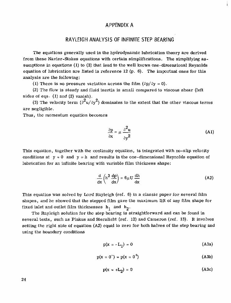
The equations generally used in the hydrodynamic lubrication heory are derived from these Navier-Stokes equations with certain simplifications. The simplifying as­sumptions in equations (1)to (3) that lead to the well known one-dimensional Reynolds equation of lubrication are listed in reference 12 (p. 6). The important ones for this analysis are the following:

(1)There is no pressure variation across the film (ap/ay = 0). (2) The flow is steady and fluid inertia is small compared to viscous shear (left

s ides of eqs. (1) and (2) vanish). (3) The velocity te rm (a2u/ay 2) dominates to the extent that the other viscous te rms

a r e negligible. Thus, the momentum equation becomes

This equation, together with the continuity equation, is integrated with no-slip velocity conditions at y = 0 and y = h and results in the one-dimensional Reynolds equation of lubrication for an infinite bearing with variable film thickness shape:

f(h3 Lp) = 6pu -&dh

This equation was solved by Lord Rayleigh (ref. 6) in a classic paper for several film shapes, and he showed that the stepped film gave the maximum lift of any film shape for fixed inlet and outlet film thicknesses hl and ha.

The Rsyleigh solution for the step bearing is straightforward and can be found in several texts, such as Pinkus and Sternlicht (ref. 12) and Cameron (ref. 13). It involves setting the right side of equation (A2) equal to zero for both halves of the step bearing and using the boundary conditions

p(x = -L1) = 0 (A34

P(X = 0-) = p(x = 0 3 (A3b)

24

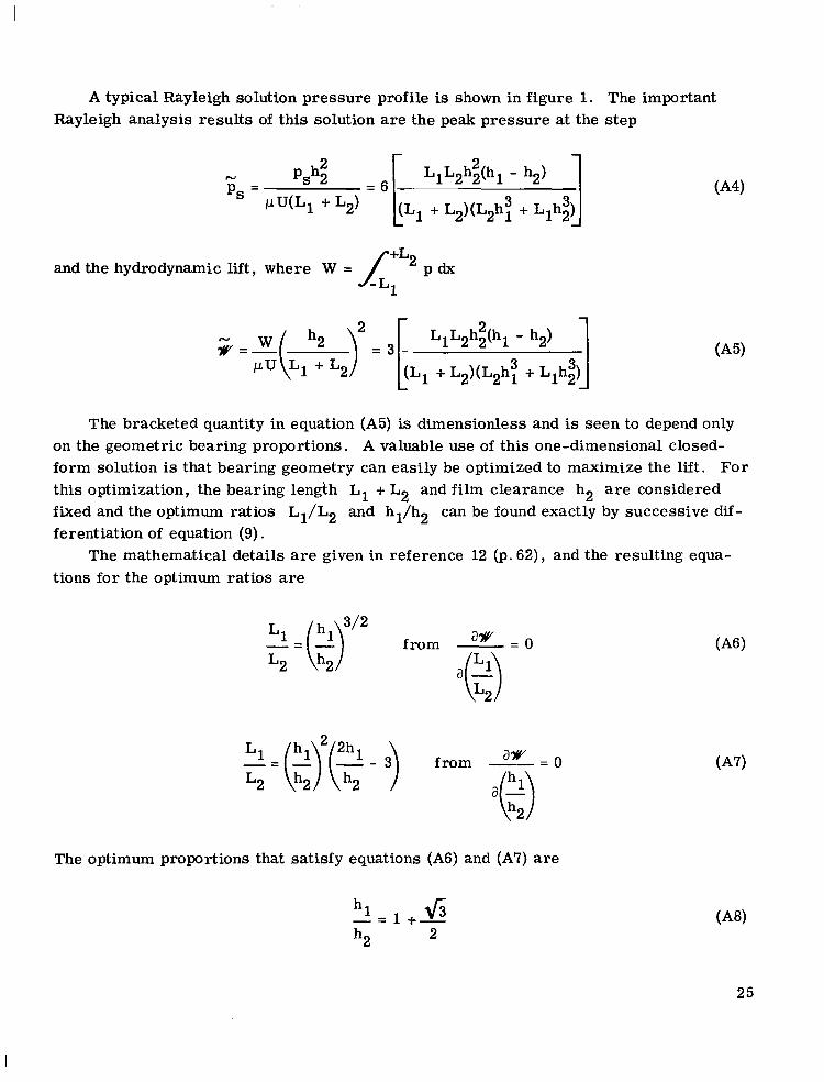
A typical Rayleigh solution pressure profile is shown in figure 1. The important Rayleigh analysis results of this solution a r e the peak pressure at the step

and the hydrodynamic lift, where W = A+L2p dx 1

The bracketed quantity in equation (A5) is dimensionless and is seen to depend only on the geometric bearing proportions. A valuable use of this one-dimensional closed-form solution is that bearing geometry can easily be optimized to maximize the lift. For this optimization, the bearing length L1 + L2 and film clearance h2 a r e considered fixed and the optimum ratios L1/L2 and hl/h2 can be found exactly by successive dif­ferentiation of equation (9).

The mathematical details a r e given in reference 12 (p. 62), and the resulting equa­tions for the optimum ratios are

from

The optimum proportions that satisfy equations (A6) and (A?) a r e

h2 2

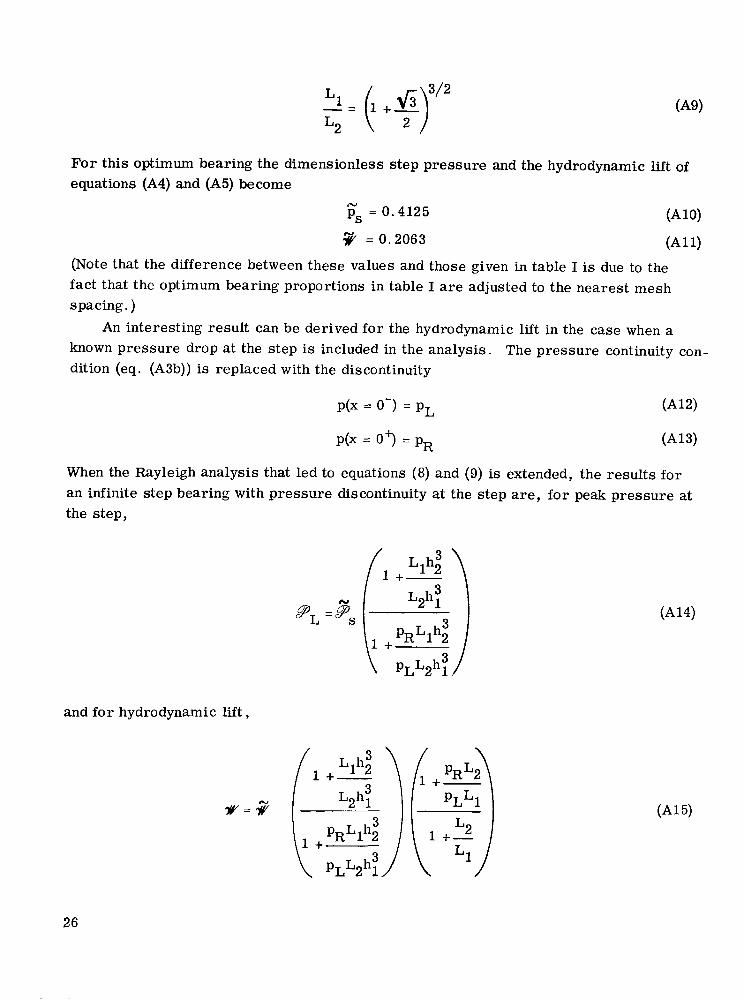
For this optimum bearing the dimensionless step pressure and the hydrodynamic lift of equations (A4) and (A5)become

Es = 0.4125

= 0.2063

(Note that the difference between these values and those given in table I is due to the fact that the optimum bearing proportions in table I a r e adjusted to the nearest mesh spacing. )

An interesting result can be derived for the hydrodynamic lift in the case when a known pressure drop a t the step is included in the analysis. The pressure continuity con­dition (eq. (A3b)) is replaced with the discontinuity

p(x = 0-) = pL (A121

p(x = 0 3 = pR (-413)

When the Rayleigh analysis that led to equations (8) and (9) is extended, the results for an infinite step bearing with pressure discontinuity at the s tep are, for peak pressure at the step,

and for hydrodynamic lift,

26

Note that, for the proportions given by equation (A6), the lift is the same as without the discontinuity at the step.

27

REFER ENCE S

1. Allen, D. N. de G. ; and Southwell, R . V. : Relaxation Methods Applied to Deter­mine the Motion, in Two Dimensions, of a Viscous Fluid Past a Fixed Cylinder. Quart. J. Mech. Appl. Math. , vol. 8, pt. 2 , 1955, pp. 129-145.

2 . Kawaguti, Mitutosi: Numerical Solution of the Navier-Stokes Equations fo r Flow in a Two-Dimensional Cavity. J. Phys. SOC.Japan, vol. 16, no. 12, Nov. 1961, pp. 2307-2315.

3. Fromm, Jacob E . ; and Harlow, Francis H. : Numerical Solution of the Problem of Vortex Street Development. Phys. Fluids, vol. 6 , no. 7 , July 1963, pp. 975-982.

4 . Harlow, Francis H. ; and Welch, J. Eddie: Numerical Calculation of Time-Dependent Viscous Incompressible Flow of Fluid with F ree Surface. Phys. Fluids, vol. 8, no. 12, Dec. 1965, pp. 2182-2189.

5. Donovan, L. F. : A Numerical Solution of the Unsteady Flow in a Two-Dimensional Square Cavity. AIAA J., vol. 8, no. 4, 1970.

6 . Rayleigh, Lord: Notes on the Theory of Lubrication. Phil. Mag., vol. 35, 1918, pp. 1-12.

7 . Constantinescu, V. N . : Lubrication in Turbulent Regime. AEC-tr-6959, 1965.

8. Osterle, Fletcher; and Saibel, Edward: On the Effect of Lubricant Inertia in Hydro­dynamic Lubrication. Zeit. f . Angew. Math. Phys . , vol. 6 , no. 4, 1955, pp. 334­339.

9 . Lyman, F. A. ; and Saibel, E . A. : Transient Lubrication of an Accelerated Infinite Slider. ASLE T r a n s . , vol. 4 , no. 1, Apr. 1961, pp. 109-116.

10. Schlichting, Hermann (J. Kestin, t rans . ) : Boundary Layer Theory. Fourth e d . , McGraw-Hill Book Co . , Inc. , 1960.

11. Kawaguti, Mitutosi: Numerical Solution of the Navier-Stokes Equations for Flow in a Channel with a Step. Rep. MRC-TSR-574, Univ. Wisconsin, May 1965. (Avail­able from DDC as AD-620108.)

12. Pinkus, Oscar; and Sternlicht, Beno: Theory of Hydrodynamic Lubrication. McGraw-Hill Book Co. , Inc . , 1961.

13. Cameron, A. : The Principles of Lubrication. John Wiley & Sons, Inc. , 1966.

28 .NASA-Langley, 1970 -12 E-5376

AERONAUTICSNATIONAL A N D SPACE ADMINISTRATION WASHINGTON,D. C. 20546

OFFICIAL BUSINESS FIRST CLASS MAIL

POSTAGE AND FEES PAID NATIONAL AERONAUTICS At

SPACE ADMINISTRATION

( ' i i i ~ I ' i * i c ( '-

1 , ' \ .', \:

If Undeliverable (Section 158 Postal Manual) Do Not Retur

"The aeroitniiticnl aizd spnce nctiiities of Ihe United Sfnfes shall be conducted so as to contribiite . . . to the expaasioiz of hiiiiiaiz knoiul­

' edge of phenoniena in the nliiiosphere aizd space. The Admivistsazion 9 shall psovide fo r the widest psacticable and appropriate dh"?ntioia .r of iaforiiintioiz comet itiiag its nctiilities aiad the vesdts thereof."

-NATIONALAERONAUTICSA N D SPACE ACT OF 1958

NASA SCIENTIFIC AND TECHNICAL PUBLICATIONS * .

TECHNICAL REPORTS: Scientific and technical information considered important, complete, and a lasting contribution to existing knowledge.

TECHNICAL NOTES: Information less broad in scope but nevertheless of importance as a contribution to existing knowledge.

TECHNICAL MEMORANDUMS: Information receiving limited distribution because of preliminary data, security classificn­tion, or other reasons.

CONTRACTOR REPORTS: Scientific and technical information generated under a NASA contract or grant and considered an important contribution to existing knowledge.

TECHNICAL TRANSLATIONS: Information published in a foreign language considered to merit NASA distribution in English.

SPECIAL PUBLICATIONS: Information derived from or of value to NASA activities. Publications include conference proceedings, monographs, data compilations, handbooks, sourcebooks, and special bibliographies.

TECHNOLOGY UTILIZATION PUBLICATIONS: Information on technology used by NASA that may be of particular interest i n coininercial and other non-aerospace applications. Publications include Tech Briefs, Technology Utilization Reports and Notes, and Technology Surveys.

Details on the availability of fhese publications may be obtained from:

SCIENTIFIC AND TECHNICAL INFORMATION DIVISION

NATI0NA L AERO N AUT1C S AND SPACE ADM IN ISTRATIO N Washington, D.C. 20546