NBER WOR~G PAPER SERIES

COMPUTER USE AND PRODUCTIVITYGROWTH IN FEDERAL GOVERNMENT

AGENCIES, 1987 TO 1992

William LehrFrank R, Lichtenberg

Working Paper 5616

NATIONAL BUREAU OF ECONOMIC RESEARCH1050 Massachusetts Avenue

Cambridge, MA 02138June 1996

We would like to acknowledge the financial support of the Sloan Foundation. Also, we wouldlike to thank the personnel at the Bureau of Labor Statistics, especially Kent Kunze and DarleneForte, who helped us access the productivity data; and Harry Henry and Chris Boehmer ofComputer Intelligence who provided us with the data on computer assets. This paper is part ofNBER’s research program in Productivity. Any opinions expressed are those of the authors andnot those of the National Bureau of Economic Research.

01996 by William Lehr and Frank R. Lichtenberg. All rights reserved. Short sections of text,not to exceed two paragraphs, may be quoted without explicit permission provided that fullcredit, including O notice, is given to the source.

NBER Working Paper 5616June 1996

COMPUTER USE AND PRODUCTIVITYGROWTH IN FEDERAL GOVERNMENT

AGENCIES, 1987T0 1992

ABSTRACT

This paper examines trends in computer usage and the effect on productivity growth for

a sample of federal government agencies over the period from 1987 to 1992. We link data from

the Bureau of Labor Statistics (BLS) on the growth in real output per employee with data from

a marketing research firm, Computer Intelligence (CI), on the growth in per capita computer

assets for a sample of 44 federal agencies. The data show that computer usage increased

dramatically and that there was a shift towards more powerful, lower cost, distributed systems

and that usage diffused more extensively throughout the sampled agencies. These trends mirror,

while perhaps lagging, those experienced by large private firms over the same period. From

estimates of a Cobb-Douglas production function for government services, we derive an estimated

output elasticity for computers of 0.06, which allows us to conclude that computers did contribute

significant y to output growth, thereby refuting the Computer Productivity Paradox as it applies

to the public sector. Computers do not appear to be responsible for the disappointing

productivity performance of the service sector. Although the magnitude of our estimated

elasticity suggests that the returns to computer investments exceeded those to other types of

capital, our results are not conclusive. We also observe a positive correlation between increased

computer usage and compensation growth which is consistent with skill-biased technical change.

William Lehr Frank R. LichtenbergGraduate School of Business Graduate School of BusinessColumbia University Columbia University3022 Broadway, Mail Code 9120 3022 Broadway, Mail Code 9120New York, NY 10027 New York, NY 10027

and NBER

1

Computer Use and Productivity Growthin Federal Government Agencies, 1987 to 1992

William H. Lehrand

Frank R. LichtenbergGraduate School of Business

Columbia University

Ver$iorz: BLSDOC. 5May 29, 1996

1. Introduction

There is a large and growing literature investigating the economic impact of computers.

Much of this work has focused on the “information productivity paradox” suggested by Robert

Solow’s quip that’” we see computers everywhere but in the productivity statistics. ” This paradox

is closely related to the more general problem of assessing service sector productivity. Business

computers are used most intensively in the service sector and in the “service” functions of non-

service sector firms (e. g., payroll and purchasing). These are exactly the activities where

economists face the most severe analytical constraints. Good data sources tracking the

productivity of services are scarce (Griliches, 1994), Accurately measuring quality-adjusted

output for services is extremely difficult. This problem is especially acute for computers because

of the rapid pace of innovation and the fact that computers and the services they support often ~

contribute only indirectly to final output. Moreover, although we may see computers

everywhere, they still represent only a tiny fraction of our capital stock (on the order of 2% of

plant, property and equipment) and so aggregate effects may be hard to detect, Recent research

which has exploited the availability of detailed firm-level panel data have been able to

successfully address some of these measurement issues and have found that computers do

contribute significantly to productivity growth and offer higher returns than investments in other

types of capital (Brynjolfswn, 1992; Lichtenberg, 1995). A related, but less well-developed

literature has found that employees who use computers are better compensated and that

computers may be enhancing the skill-based wage gap (Kreuger, 1993). While these results are

both important and interesting, they focus exclusively on the private sector and tend to over-

2

emphasize manufacturing.

This paper presents

shared by the public sector.

initial evidence that private sector experiences with computers are

This is interesting both because the federal government is the single

largest service sector employer and because of its long-established role in promoting the

development and deployment of advanced technologies. It is especially interesting in light of the

recent controversy over public policies affecting the development of the Information

Superhighwq.2 We use data from the Bureau of Labor Statistics (BLS) on the growth in real

output and compensation per employee and data from a private market research firm on the

growth in computer assets for the period 1987-1992. These data show that computer use

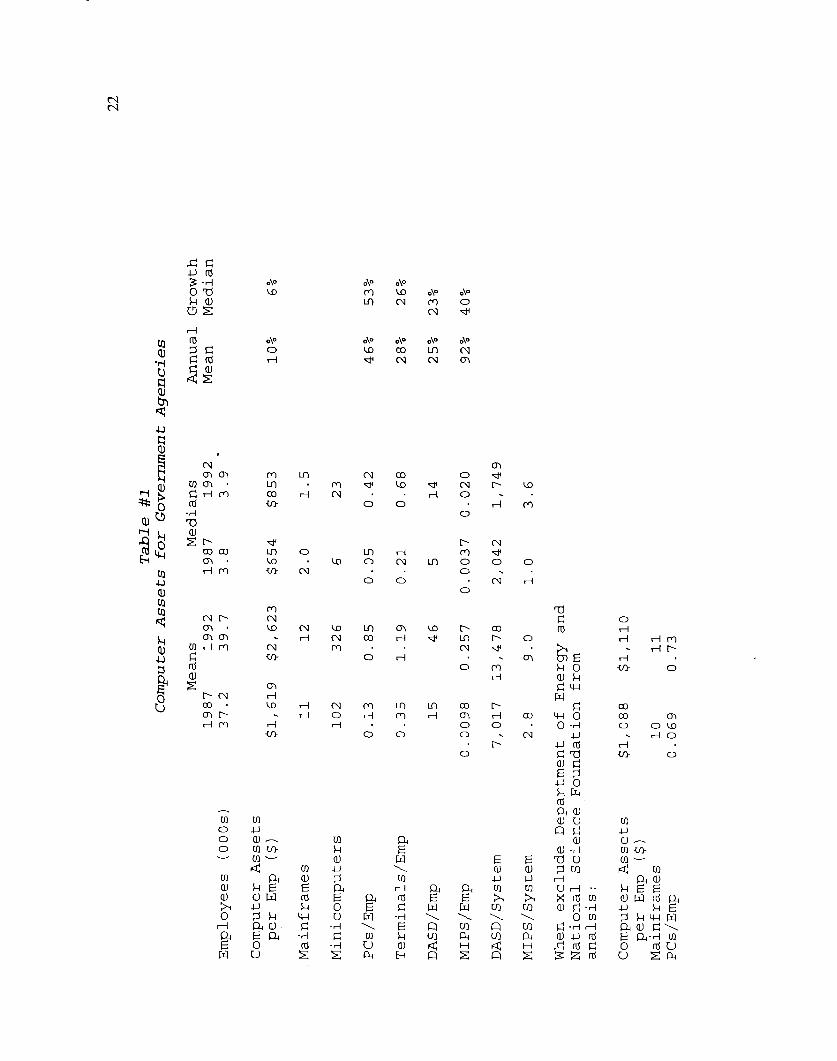
increased dramatically over the study period (see Table #1). The median value of computer

assets per employee increased 5 % per year, and there was a strong trend towards increased,

reliance on distributed systems based on PCs and terminals (e, g., PCs per employee, MIPS per

employee and DASD per employee grew at 53%, 40% and 23% per year, respectively).3 We

find that this increased computerization contributed positively to productivity growth, even

though growth in output per worker was disappointingly low, averaging 0.2 % per year.4 We

also find that compensation per employee grew more rapidly in the computer intensifying

2 The recent passage of the telecommunications deregulation bill in the US and similar regulatory trends -

in other OECD countries reflects the growing belief that global competitiveness will depend heavily on the stateof a count~y ’s information infrastructure. This only makes sense if computers contribute positively to economicgrowth,

3 These are growth rates for the medians. See Table #1.

4 By way of comparison, from 1985 to 1992, output per labor hour and compensation per labor hour for

private-sector manufacturing grew 2.8 % and 4.2%, respectively (see Statistical Abstract 1994, Table 1390).Over the same period, the comparable numbers for the Federal agencies surveyed by the Bureau of LaborStatistics increased O,2 % and 5,9%, respectively (see Productivity Statistics for Federal Government Functions,Bureau of Labor Statistics, February 1994, page 1). For the 44 agencies which are included in our regressionanalysis the comparable means are:

Average Annual Growth RatesOutput per CompensationEmployee year per Employee year

Simple means 1.2% 6.3%Mean weighted by BLSSHR 1.2 6.3Mean weighted by employment O .4 6.3

3

agencies, which is consistent with skill-biased interpretations of computerization. 5

Section 2 describes our data in greater detail and Section 3 presents our results and

Section 4 offers our summary conclusions.

2. Data Description

We use data on the growth in productivity and computer assets for a subset of U.S,

federal agencies over the period 1987-1992, The productivity data are from the Bureau of Labor

Statistics’ (BLS) Federal Productivity Measurement Program. Since 1967, the BLS has been

compiling output, employment and compensation indices for a significant share of the activities

undertaken by the federal government. b This research program is noteworthy for both its

extensiveness and for the care taken to accurately measure real output over a long period. In,

1992, the study covered 276 government organizations which are part of 60 Federal agencies

representing almost 65% of executive branch employment.

The BLS analysts took great care defining the real output for the government

organizations which are included in their survey. Output measures were derived in close

consultation with personnel in the target organizations and vary depending on the function of the

organization, For example, output for the postal service is measured as the growth rate in the

volume of mail handled, with different indices for each type of mail and indices for the number “

of money orders sold. For the forest service, output is measured for 28 different activities

including the acres managed for wilderness management or the publications issued for forest

research.

5 Growth in compensation per employee for firms was positively correlated with the growth in PCs and

terminals per employee, but not with the relative intensity of computer usage in the initial year as measured bythe ratio of the number of PCs and terminals per employee for the firm relative to the industry mean in 1987,

6 See Productivity Statistics for Federal Government Functions: Fiscal Years 1967-1992 (Febmary 1994),

and, Description of Output Indicators by Function for the Federal Government (March 1994) from the Bureauof Labor Statistics, U.S. Department of Labor, for additionat information, Also, Forte (1993).

4

The BLS publishes data in the form of aggregate statistics for 28 different government

functions such as “audit of operations”, “traffic management”, and “communications”. Each of

these functional indices is computed by aggregating a series of output measures for each of the

sampled organizations which are engaged in activities associated with that function, For example,

the “audit of operations” index is based on data for organizations in three different agencies. One

of these is the Office of the Inspector General in the Department of Labor for which output is

measured as the number of audits completed. The BLS program collects information on

approximately 2,500 different activities. The activity indices are aggregated to produce functional

indices and agency-level indices based on base-year employment weights. Although the BLS does

not publish the agency-level aggregate indices, we were able to use these in our analysis.7 In

addition to computing the growth in output per employee year, the BLS collects data on total

employment and the growth in compensation per employee year for the sampled organizations,

The data on computer assets by agency comes from the market research firm, Computer

Intelligence (CI), which conducts site-level surveys of total employment and computer asset

inventories for Federal government agencies. The computer asset data includes an estimate of

the replacement value of computer assets (CPURCH) as well as physical counts of such things

as the number of mainframes, minicomputers, PCs, terminals, total MIPS, and total disk

storage (DASD),

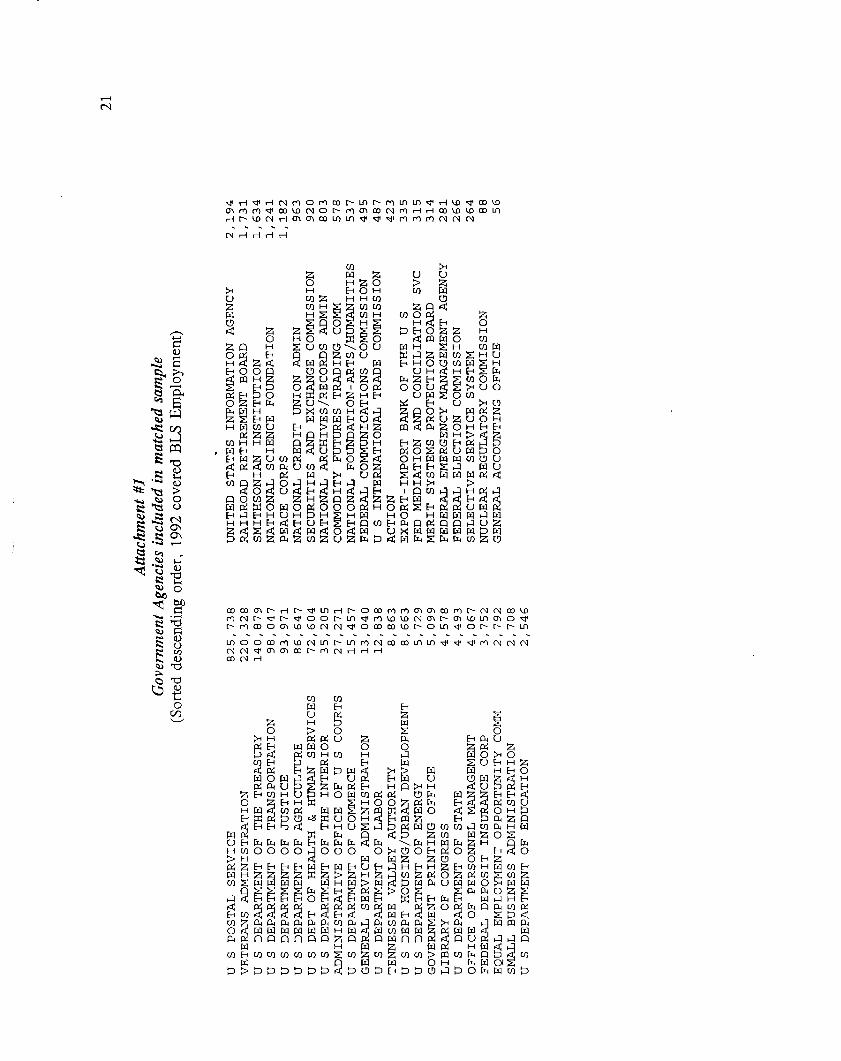
The CI data were aggregated to the agency level and matched to the BLS agency-level

agencies, covering almost 80% of the

for a list of agencies included in the

the two data sources at the organization

productivity statistics, resulting in a data set with 44

employment in the BLS sample. (See Attachment #1

sample. ) Originally, we had hoped to be able to match

level, which would have resulted in a much larger sample. Unfortunately, the only information

we could match on was the name of the

matches.

site/organization which did not generate reliable

7 The BLS protects the confidentiality of the organization and agency-level indices as part of its

agreement with the departments which participate in the survey,

5

Since the BLS surveyed only a subset of the organizations within an agency, its coverage

is partial (ranging from 1% to 100% of agency employment), while the CI data (in principle)

reflect 100 % agency coverage. Also, the time periods covered by the two samples do not match

perfectly. The BLS data we use are from 1987 and 1992, while the CI data are from 1986 and

1991,8 This creates a matching problem across the two data sources which is reflected in our

inability to perfectly match total agency employment in the two samples. The average

employment-weighted BLS coverage ratio in our sub-sample is 0.84 and the average ratio of

BLS employment to CI employment is 0.88. Ideally, these numbers should both be 1, or at least

equal. However, their closeness encourages us to assume that the matching problem is not

severe,

The mismatch in coverage ratios may be interpreted in a variety of ways. First, we may

assume that the BLS productivity index offers an unbiased estimate of total agency productivity

growth. In this case, we would wish to compare the growth in agency-level computer intensity

with agency-level productivity growth. Alternatively, we may assume that the average agency-

level computer intensity provides an unbiased estimate of computer intensity in those

organizations sampled by the BLS. 9 The partial coverage of BLS data suggests that our estimates

of agency productivity may be heteroskedastic. The variance of our estimate of productivity

growth should be inversely related to the BLS coverage ratio (BLSSHR), It would be largest for

agencies for which BLSSHR is small. We adjust for this potential measurement error by using

BLSSHR to weight observations in the regressions.

To correct for the timing difference, we convert all growth rates into annual growth rates

and assume that average annual growth was approximately the same over the two periods,

Finally, to further correct for potential measurement problems imposed by matching across the

a The CI data are from 1986 and 1991, with a few of the second observations from 1990 and 1992,

9 From the site-level data, we may infer that computer intensity varies quite a lot across different

organizations in an agency (e. g., the CV in average agency epurch is 2,2). This makes intuitive sense since wemight expect certain agency functions to be more computer intensive than others (e. g., researchers versus parkrangers in the Department of Agriculture), This suggests that the first assumption is perhaps more plausible.

6

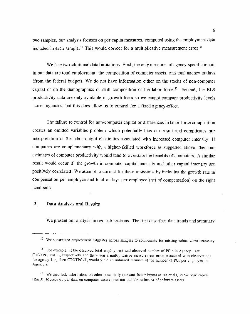
two samples, our analysis focuses on per capita measures, computed using the employment data

included in each sample. 1°This would correct for a multiplicative measurement error, 11

We face two additional data limitations. First, the only measures

in our data are total employment, the composition of computer assets,

of agency-specific inputs

and total agency outlays

(from the federal budget). We do not have information either on the stocks of non-computer

capital or on the demographics or skill composition of the labor force. 12 Second, the BLS

productivity data are only available in growth form so we cannot compare productivity levels

across agencies, but this does allow us to control for a fixed agency-effect.

The failure to control for non-computer capital or differences in labor force composition

creates an omitted variables problem which potentially bias our result and complicates our,

interpretation of the labor output elasticities associated with increased computer intensity. If

computers are complementary with a higher-skilled workforce as suggested above, then our

estimates of computer productivity would tend to overstate the benefits of computers, A similar

result would occur if the growth in computer capital intensity and other capital intensity are

positively correlated. We attempt to correct for these omissions by including the growth rate in

compensation per employee and total outlays per employee (net of compensation) on the right

hand side,

3. Data Analysis and Results

We present our analysis in two sub-sections. The first describes data trends and summary

10 We substituted employment estimates across samples to compensate for missing values when necessary.

11 For example, if the observed total employment and observed number of PC’s in Agency i are

CTOTPCi and Li, respectively and there was a multiplicative measurement error associated with observationsfor agency i, cl, then CTOTPCi/L, would yield an unbiased estimate of the number of PCs per employee inAgency i.

12 We also lack information on other potentially relevant factor inputs as materials, knowledge capital

(R&D). Moreover, our data on computer assets does not include estimates of software assets.

7

statistics, contrasting public and private sector experiences. The second part discusses our

regression analysis of the relationship between increased computerization and productivity and

compensation growth.

3.1 Trends and Data Patterns

From 1987 to 199213, the output per employee year grew at only 0.2 % per year while

compensation per employee year grew 5,9 % for the agencies included in the BLS survey. This

disappointing performance was shared by the private service sector. The expansion of the service

sector’s share of GDP coupled to its disappointing performance threaten fiture economic growth

and help account for the strong interest in better understanding the causes for low measured

productivity growth, 14 It is worth noting that while overall growth was slow, certain functions,

experienced quite rapid growth, For example, communications grew 7.9 % per year while

procurement declined (3. 5%) per year, 15 Other functions which experienced relatively rapid

growth included traffic management (+18 %/year), electric power and distribution (+7.4 %/year)

and personnel investigations (+4, 9%/year); while functions for which productivity declined

included legal and judicial activities (-1. 7%/year), education and training (-2, O%) and personnel

management (-2, 2%). Similarly, there is a wide range in the productivity growth rates for the

13 As noted above, the timing of our two data sources are not identical, The BLS data are calendar years

1987 and 1992, while the Computer Intelligence data are for calendar years 1986 and 1990-1992 with thefollowing frequencies. 48 agencies 1986, 3 agencies 1990, 42 agencies 1991 and 3 agencies 1992. To simplifythe exposition, we will treat all of the data as from either “1987” or “1992” in subsequent discussions andtables.

14 Over approximately the same period, employment in the Federal government grew at only one third

the rate of the economy as a whole (0.5% versus overall growth of 1,4% per year from 1979 to 1992).

According to the Statistical Abstract of United States, Table 642: Employment by Selected Industry,

Annual Growth Share ofEmployment Emplo~ent1979-1992 1979 1992

Federal Govt 0.5 2.3% 2.5%State and Local Govt 1.4 13.0 13.0Services, overall 2.3 16.6 23.5Total 1.4% 100.0% 100.0%

15 Average annual growth in output per employee year from 1987 to 1992.

8

organizations from which the functional indices are computed. For example, output for the

organizations which contribute to the index for information services (overall growth of 2.2 % per

year) ranged from a decline of (3.8%) per year to an increase of 26 % per year. 16

Over this same period, computerization of public sector work places continued at a rapid

pace (see Table #1). Although all of the agencies in our sample owned computers in 1987,

changes in the numbers, value and composition of the equipment were substantial. 17The median

replacement value of computer assets per employee grew 5.5% per year to about $853 per

employee in nominal terms, which suggests real growth of 25 % to 35 YOper year since computer

prices have been declining rapidly. 18

In Table #2, we report regressions results which show how the total replacement value,

of computer assets in 1987 and 1992 varies with the number of different types of systems. The

parameters may be interpreted as estimates of the average system prices in 1987 and 1992. Our

data show that the average replacement price for PCs fell by 10% per year from approximately

$2,300 to $1,300, while the price for terminals fell by 23% per year. Since the quality of

systems purchased tended to increase over time, these estimates understate the fall in real prices,

According to data from Multimedia Computing Corporation, the average price for a government

computer was $2,500 in 1989, which is encouragingly close to our estimate in Table #2.’9

16 The BLS publishes the range of organizational indices only if there are three or more organizations

which contribute to the determination of the functional index so that it is not possible to identify individualorganizations.

17 Of the 48 agencies in our sample, 13 do not have mainframe computers in either or both years.

However, 10 of those have minicomputers and all 48 have at least PCs or terminals in both years.

16 Berndt, Griliches, and Rappaport (1993) estimate that computer prices declined on average 20% to

30% per year from 1989 to 1992, Nominal prices declined 1] % per year, but changes in model specifications

and quality mask much steeper real price declines. When quality adjusted, the indices fall 24% 10 32%, Theiranalysis is based on personal computers.

19 See page 10.17 in Juliussen and Juliussen (1991). And, according to data from the Computer Business

Equipment Manufacturers Association (CBEMA), the average price for a microcomputer, minicomputer and a

mainframe in 1987 were $2.4k, $57k and $1, 100k, respectively (Ibid, see page 10.8). According to the

CBEMA data, the Wares of total domestic shipments of micros, minis and mainframes were 38%, 25% and

9

This intensification in the level of computerization was accompanied by a shift in the

types of computers used, and implicitly, in the ways in which computers are used within the

organization. While mainframes remained important, the growth in PCs and terminals suggests

that computer use was diffising more widely across the agencies. In our sample, the mainframe

plus terminal share of asset value declined from 57% to 34%, while the share of asset value

attributed to PCs increased from 1570 to 40 YO(see Table #2). Over the same period, the median

number of PCs per employee, MIPS per employee and DASD per employee grew rapidly, at

53%, 40% and 23% per year, respectively (see Table 1).20 Also noteworthy are the increase in

MIPS per system and the decrease in DASD per system. The former attests to the dramatic

increase in computing power, while the latter provides additional evidence of the trend towards

distributed systems.

,

Almost all of the agencies in our sample increased the number of minicomputers per

employee, PCs and terminals per employee, MIPS per employee and DASD per employee; while

almost half did not change the number of mainframes and almost a third decreased the share of

mainframes .21 This provides evidence of the move towards distributed computing environments

with computer technology diffusing throughout the agency. During the same period, the number

of agency locations/sites per employee increased for 8870 of the agencies in our sample. It seems

plausible that the move towards a more geographically distributed organizational structure was

facilitated in part by the increased deployment of computer technology.

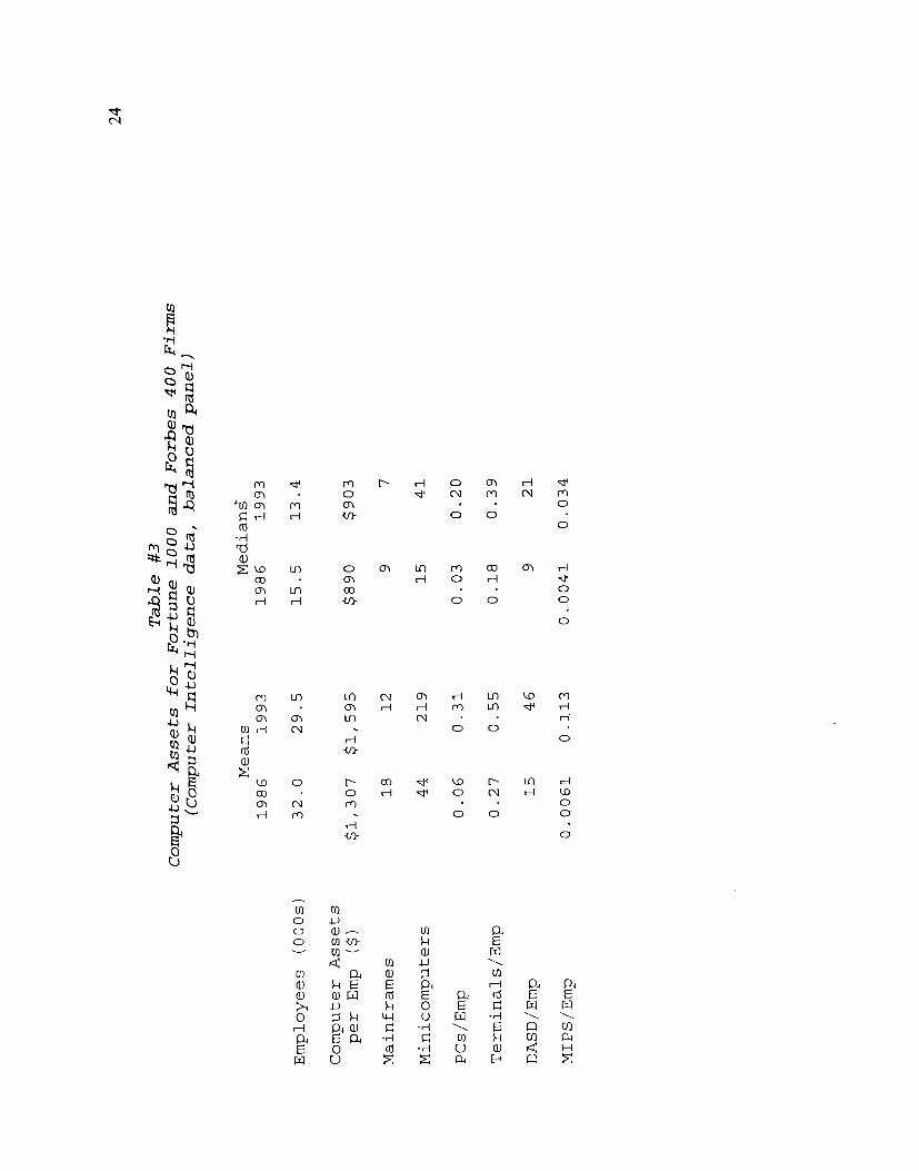
The patterns in computer utilization are quite similar to those experienced by the private

37% respectively. In comparison with the estimates in Table #2, these estimates imply penetration rates for

mainframes which are lower than ours and for PCs which are higher (i. e., lumping terminal shares withmainframes). Since the CBEMA data include the private sector and reports domestic shipments, we would expect tile data to

differ in this way if the private sector is more computer intensive than the public sec[or.

20 These are median growth rates computed using CUPDATE to determine the length of time between

observations.

21 Share of agencies which increased units per employee (among those which report data): PCs (100% ),.

Terminals (98 %), MIPS (93 %), DASD (95%). Of those firms with mainframes in both sample years, 48% do

not change, 2970 decrease and 2370 increase the number of mainframes.

10

sector over the same period (see Table #3). The data on private sector firms is from Computer

Intelligence also, and covers Fortune 1000 and Forbes 400 firms. A comparison of median

values suggests that the government agencies were less computer intensive than private sector

firms .22 Government agencies had fewer mainframes, minicomputers, DASD and MIPS per

employee, but more PCs and terminals. These differences do not appear due to the significantly

smaller median size of government agencies, since scale effects ought to work in the opposite

direction. These results are intriguing in that they suggest that the government’s role in

encouraging the diffusion of computer technology has not acted principally via their role as

“pioneer-buyers” or as benevolent “monopsonists”. Thus, if the government has been

instrumental in encouraging the development or diffusion of technology, it seems more likely

to have worked either via R&D funding, the standards process, or some other avenue.

Unfortunately, the present data sample does not provide sufficient information for us to derive

much confidence from these speculative observations. The present sample excludes the

Department of Defense and contains only limited information on the relative timing and

magnitude of government versus private sector investments.

3.2 Regression Results

We examined the relationship between government productivity, compensation and “

computers formally by estimating several reduced-form regressions. Our results are discussed

in the two following subsections. The first examines the relationship between productivity

growth and computers and the second explores the relationship between computers and growth

in employee compensation,

22 Comparim of means is less valuable since there are several important outliers in the government

sample. These include the Department of Energy (Corp =2004) an the National Science Foundation(Corp =2034), both of which are very computer intensive and both of which are arguably close to being pureR&D organizations. When these agencies are excluded, the sample mean for computer assets per employee in

1992 falls to $1,110 and the number of PCs per employee falls to 0.07 in 1987 and 0,73 in 1992. This latter

estimate suggests that the observation that PCs were used relatively more intensively by the public sector isrobust.

11

i. Productivity Growth and Computers

If computers enhance productivity, then we should expect to see a positive correlation

between the level of computerization and growth in productivity. Production theory provides us

with a theoretical basis for deriving our estimating equation. We should expect real output (Y)

to be an increasing function of capital (K) and labor inputs (L). The capital inputs could be

divided into computer capital (Kl) and other capital ~). The CI data provide estimates of KI,

but ~ is not observed. The labor inputs should also be divided into skilled (~) and unskilled

labor (Lu) so that we can control for differences in the quality of an agency’s labor force. The

effective level of labor inputs, L* = LU + (1+ 8)L~, where 6 measures the excess productivity

of skilled workers and should be equal to their wage premium over unskilled workers.

Unfortunately, we only observe total employment (L = ~ +Lu). If we approximate the production

function for “government services” by a Cobb-Douglas function, we obtain the following (in log

form) :

h-l(q) = y, + ai + alln(K1,iJ + aoln(Ko,iJ + aLln(Lu,it +(1 +e)L~,i) + pit (1)

The parameter y, measures disembodied technological change, ~ is a fixed effect which captures

agency-specific differences, and ~,, is a random error with zero mean which captures the effect

of all other unobserved variables which contribute to the determination of real output. (To

simplify the notation, we will drop the i and t subscripts, )

After assuming constant returns to scale so al+ aO+ aL = 1 and converting to per capita

estimates, we obtain the following:

(2)

If the share of skilled workers is small (~/L is 10% or less), then this further simplifies to:

in(:) = y + A + alln(:)+sob(:)+aLe;+p

12

(3)

This can be written in growth rates as:

KOln(;)92-hl(:)87 “ y + u1(hl(+)92-hl(; )87) + ao(ln(:)92-ln(= )*7)

(4)

+ aL6((;)92-(;)87)+(P9*- Pg~),

Converting to growth rates eliminates the agency-fixed effect and the intercept term, y, should

now be interpreted as the growth in the technical parameter. The BLS data provide a measure

of the growth rate in real output per employee (PROD92) and the CI data provide a measure of

the replacement value of computer assets per employee (EPURCH). We do not observe either

~ or L~/L, but if the capital-labor ratio for non-computer capital and the share of skilled labor

do not change over time or are not correlated with the computer capital to total labor ratio, then

the second and third terms drop out, and we are left with our basic estimating equation:

ln(l +growth(PR0D92)) = y+ a ~ln(l +growth(EPURC~) + ~ ~ (5)

Table #4 shows a scatter plot of the growth rate in output per employee (PR0D92) versus the

growth rate in the value of computer assets per employee (EPURCH). From the plot, it appears

that PROD92 is positively correlated to EPURCH, as expected. The regression results presented

in Table 5 confirm that this result is significant and large. The balance of this section discusses

each of these regressions in greater detail and further refinements which support this basic

finding.

13

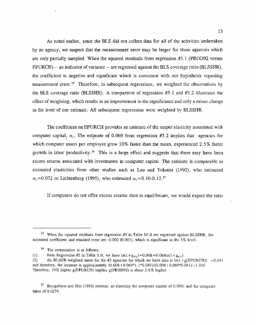
As noted earlier, since the BN did not collect data for all of the activities undertaken

by an agency, we suspect that the measurement error may be larger for those agencies which

are only partially sampled. When the squared residuals from regression #5. 1 (PROD92 versus

EPURCH) --an indicator of variance -- are regressed against the BLS coverage ratio (BLSSHR),

the coefficient is negative and significant which is consistent with our hypothesis regarding

measurement error.23 Therefore, in subsequent regressions, we weighted the observations by

the BLS coverage ratio (BLSSHR). A comparison of regression #5.1 and #5.2 illustrates the

effect of weighting, which results in an improvement in the significance and only a minor change

in the level of our estimate. All subsequent regressions were weighted by BLSSHR.

The coefficient on EPURCH provides an estimate of the output elasticity associated with

computer capital, crl. The estimate of 0.069 from regression #5.2 implies that agencies form .

which computer assets per employee grew 10% faster than the mean, experienced 2.5 YOfaster

growth in labor productivity .24 This is a large effect and suggests that there may have been

excess returns associated with investments in computer capital. The estimate is comparable to

estimated elasticities from other studies such as Lau and Tokatsu (1992), who estimated

al =0.072 or Lichtenberg (1995), who estimated al =0. 10-0.12.25

If computers do not offer excess returns then in equilibrium, we would expect the ratio

23 When the squared residuals from regression #1 in Table $4 .B are regressed against BLSSHR, the

estimated coefficient and standard error are -0.002 (O,001), which is significant at the 5 % level,

24 The computation is as follows:

(1) from Regression #2 in Table 5 B, we have ln(l +gY,~) =0.008 +0.0691n(l +gK,~)

(2) the BLSHR-weighted mean for the 43 agencies for which we have data is ln(l +g(EPURCH)) =0,041and therefore, the increase is approximately (0.008+0.069*1. 1*0.041)/(0.008 +0.069*0.04 1) = 1,026Therefore, 10% higher g(EPURCH) implies g(PROD92) is about 2,6% higher.

25 Brynjolfson and Hitt (1993) estimate an elasticity for computer capital of 0.0061 and for computer

labor of 0,0274.

14

of the elasticity of computer capital to other capital to be equal to the ratio of expenditure shares,

or:

al RIK1—. — (6)

“O ROKO

where Ri is the rental price for ~ and ~i is the elasticity. According to Lichtenberg (1995~b,

this implies that al= aO(O.108). Since capital’s share of total expenditures is around 30%, this

suggests that al ought to be about 0.03. Hence, our estimate of 0,069 which is over twice as

large implies that computer capital yields excess returns .27

In Regression #3, we

coefficient. The coefficient on

include employment growth and find a significant negative

employment growth (CEMPLE) of -0.287 means that agencies

whose employment grew 10% faster relative to the mean firm, experienced approximately 2.0 %

slower productivity growth. This result is compatible with a number of interpretations. First, it

is possible that there are short-run decreasing returns to scale (e. g., because adjustment costs are

large). This is the opposite of what occurs in the private sector where we find that productivity

tends to be pro-cyclical (since labor costs are quasi-fixed).

Alternatively, it may be the case that productivity growth is exogenous and both the

demand for computers and employment are endogenous. Agencies choose the mix of computers

26 Lichtenberg (1995) derived the estimate that al= aO(RIK1/~) = O.108a0 using private sector data as

follows. First, Lichtenberg noted that computer’s comprised 1.8% of total capital assets, or(P, K,)/(P~) =0.018. The relative asset prices can be converted to relative rental prices by multiplying by(R+5,-E(p,))/(R +60-E(pO)) where R is the interest rate, 8, is the depreciation rate, and E(p,) is the expected

rate of price appreciation, Lichtenberg followed Lau and Tokatsu (1992) who used long run averages to estimate

R= O.07, 6,=0,20, 8.=0.05, E(pl) =-0.15, and E(pO)=0.05. Taken together, these imply that the ratio of

relative rental to asset prices, is 6 = (,07 +.20+.15)/(.07+.05-,05), or RIK1/~=6(0,018) =0, 108.

27 However, a test of excess returns is not significant at the 10% level. The test HO: al-O .03=0 for

regression #5.2 is rejected ordy at the 10.6570 level. Since Lichtenberg’s estimate is based on private sectordata, it would be better to develop a test based on govermnent data.

15

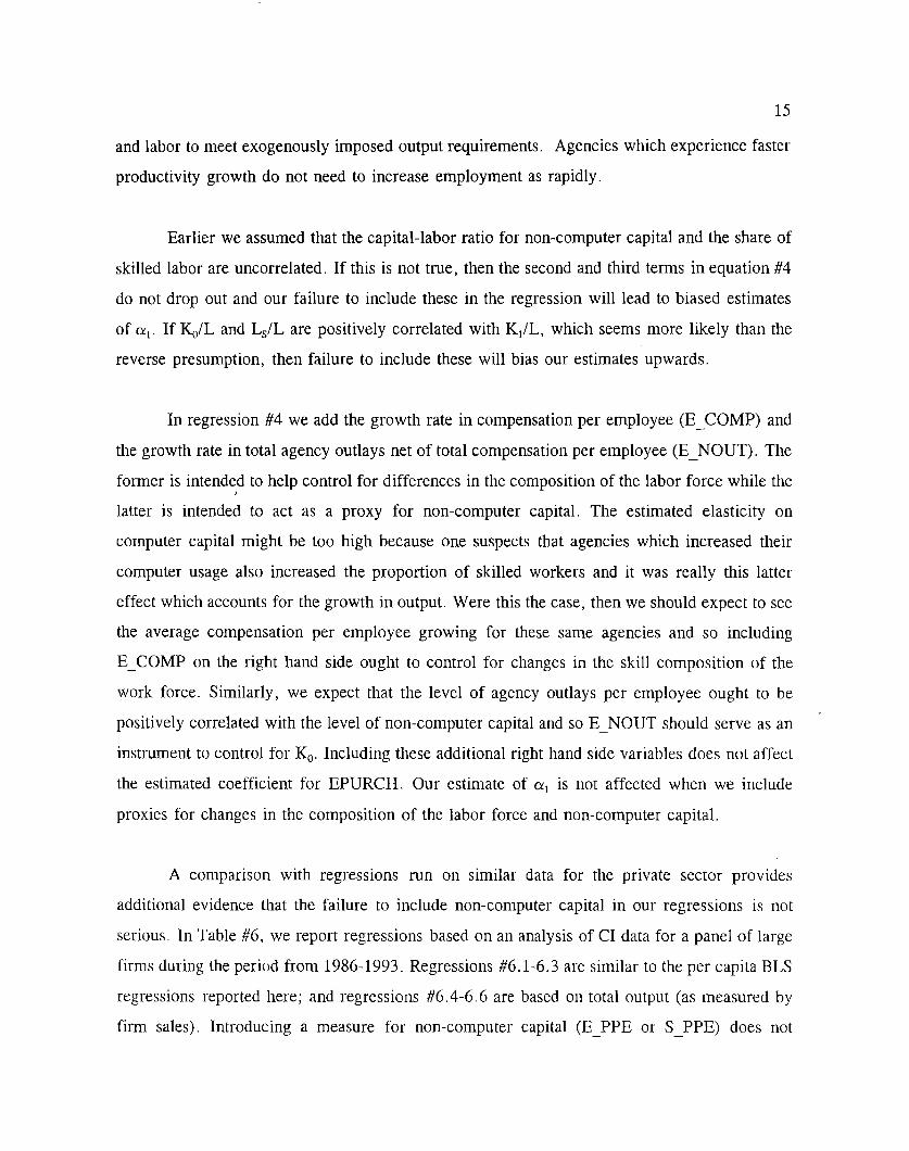
and labor to meet exogenously imposed output requirements. Agencies which experience faster

productivity growth do not need to increase employment as rapidly.

Earlier we assumed that the capital-labor ratio for non-computer capital and the share of

skilled labor are uncorrelated. If this is not true, then the second and third terms in equation #4

do not drop out and our failure to include these in the regression will lead to biased estimates

of U1. If ~/L and L~/L are positively correlated with K1/L, which seems more likely than the

reverse presumption, then failure to include these will bias our estimates upwards.

In regression #4 we add the growth rate in compensation per employee (E_COMP) and

the growth rate in total agency outlays net of total compensation per employee (E_NOUT). The

former is intended to help control for differences in the composition of the labor force while the,

latter is intended to act as a proxy for non-computer capital. The estimated elasticity on

computer capital might be too high because one suspects that agencies which increased their

computer usage also increased the proportion of skilled workers and it was really this latter

effect which accounts for the growth in output. Were this the case, then we should expect to see

the average compensation per employee growing for these same agencies and so including

E_COMP on the right hand side ought to control for changes in the skill composition of the

work force. Similarly, we expect that the level of agency outlays per employee ought to be

positively correlated with the level of non-computer capital and so E NOUT should serve as an “

instrument to control for ~. Including these additional right hand side variables does not affect

the estimated coefficient for EPURCH. Our estimate of al is not affected when we include

proxies for changes in the composition of the labor force and non-computer capital.

A comparison with regressions run on similar data for the private sector provides

additional evidence that the failure to include non-computer capital in our regressions is not

serious, In Table #6, we report regressions based on an analysis of CI data for a panel of large

firms during the period from 1986-1993. Regressions #6. 1-6.3 are similar to the per capita BLS

regressions reported here; and regressions #6.4-6. 6 are based on total output (as measured by

firm sales), Introducing a measure for non-computer capital (E_PPE or S_PPE) does not

16

significantly change the estimated computer capital output elasticity of approximately 0.03, Note

that this elasticity is smaller than the one estimated in the BLS regressions, and following the

earlier reasoning, would suggest that there are not excess returns associated with computer

capital in the private sector. This is at variance with the findings in Lichtenberg (1995) which

may be due to changes between 1991 and 1993. Since these results are preliminary, however,

we should regard these estimates with caution.

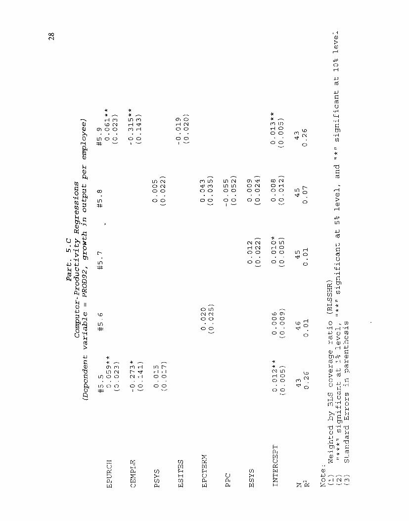
In Regressions #5.5 through #5.9, we introduce additional information from the

Computer Intelligence data on the composition of computer capital. None of these additional

regressors are superior to EPURCH nor are they significant when added to Regression #3. In

Regressions #5 through #8, we experiment with a variety of ways of measuring changes in

computer factor inputs. The Computer Intelligence data provide a wealth of information on the,

counts of different types of computer assets which suggests that it might be possible to use this

information to detect how the composition of computer assets influences productivity, We

include such measures as the share of all systems which are large systems (PSYS), the share of

total PCs and terminals which are PCs (PPC), the total number of PCs and terminals per

employee (EPCTERM), and the total number of large systems per employee (ESYS), None of

these experiments resulted in significant coefficients .28

The failure of these regressions to yield interesting results is not especially surprising. “

The counts of systems are an extremely coarse indication of the composition of computer assets,

This is more true for mainframes and minicomputers than it is for microcomputers since the

latter are more of a commodity product. Moreover, since mainframes and minicomputers are

much more expensive than PCs or terminals, investments are lumpier and we are more likely

to face an integer problem. Growth rates for many of the alternative measures are strongly

positively correlated. This is especially true for the value of computer assets per employee

(EPURCH) and the number of MIPS per employee (EMIPS) or the number of minicomputers

28 When included, the coefficients on the MIPS per employee (EMIPS), disk storage per employee

(EDASD) or the share of large systems which are mainframes (PMAIN) were also not significant.

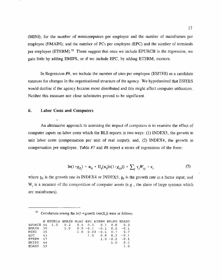
17

(MINI); for the number of minicomputers per employee and the number of mainframes per

employee (EMAIN); and the number of PCs per employee (EPC) and the number of terminals

per employee (ETERM) .29 These suggest that once we include EPURCH in the regression, we

gain little by adding EMIPS, or if we include EPC, by adding ETERM, etcetera.

In Regression #9, we include the number of sites per employee (ESITES) as a candidate

measure for changes in the organizational structure of the agency. We hypothesized that ESITES

would decline if the agency became more distributed and this might affect computer utilization.

Neither this measure nor close substitutes proved to be significant,

ii. Labor Costs and Computers

An alternative approach to assessing the impact of computers is to examine the effect of

computer inputs on labor costs which the BLS reports in two ways: (1) INDEX5, the growth in

unit labor costs (compensation per unit of real output); and, (2) INDEX4, the growth in

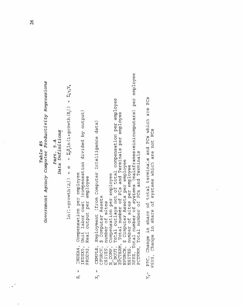
compensation per employee. Table #7 and #8 report a series of regressions of the form:

(7)

where gz is the growth rate in INDEX4 or INDEX5; & is the growth rate in a factor input; and

Wj is a measure of the composition of computer assets (e, g., the share of large systems which

are mainframes).

29 Correlations among the ln( 1+ growth rate(Xi)) were as follows:

N EPURCH EMAIN MINI EPC ETERM EMIPS EDASDEPURCH 44 1.0 0.2 0.5 0.1 0.1 0.6 0.3EMAIN 35 1.0 0.5 -0.1 -0.1 0.2 -0.1MINI 35 1.0 0.03 -0.1 0.7 0.7EPC 43 1.0 0.8 0.2 -0.1ETERM 47 1.0 -0.2 -0.1EMIPS 44 1.0 0.4EDASD 39 1.0

18

are mainframes).

Since an agency’s labor demand and production decisions are intimately related, the

analysis discussed here should complement, and partially, duplicate the earlier discussion. It is

useful in the present context because it offers an additional check on data consistency, and more

importantly, it seems to offer better insight into the effects of the composition of computer assets

as will be discussed further below. The reason for this is that we know more about the labor

force of government workers and employment/compensation trends than we do about the

heterogeneity in the outputs and productive activities of goverment services.

If computers enhance labor productivity, then they should reduce unit labor costs

(INDEX5). The results in Regressions #7.1 through #7.4 show this to be the case: the coefficient

on the replacement value of computer assets (CPURCH or EPURCH) is negative and significant.

Focusing on Regression #7.4, 10% faster growth in computer assets per employee (EPURCH)

resulted in 0.6 % slower growth in unit labor costs; while 10% faster growth in employment

(CEMPLE) increased the growth in unit labor costs by 0.5%. The negative coefficient on

EPURCH suggests that computers do indeed enhance labor productivity, mirroring the results

presented above.

The positive (though statistically not significant) relationship between average unit labor

costs and total terminals and PCs (EPCTERM) in Regression #7,4 is likely to be due in part

to the positive skill bias associated with computer use. While EPURCH provides the best

measure of an agency’s overall factor commitment to computers, a high value for EPURCH may

be due to a few employees using expensive mainframe machines or many employees using less-

expensive desk-top devices, The variable EPCTERM addresses this issue and since we know that

income and computer use are strongly correlated in the population at large, we may conclude

that organizations with high EPCTERM are likely to have a larger share of higher-skilled,

higher-paid employees. These results offer further support for the view that computers are

complementary ‘with higher skilled labor.

19

The positive coefficient on employment indicates that organizations that increased

headcount more quickly, increased unit labor costs more quickly also. This is inconsistent with

a view of technological progress where a few highly-skilled computer workers replace a large

number of less-skilled workers in completing the same tasks. It is consistent with a shift towards

higher-skilled activities, which are also likely to be more computer-intensive.

Regressions #8. 1 through #8,3 examine the effects of computers on the growth in average

compensation (INDEX4). First, the skill-biased nature of employment growth observed above

is further supported here by the positive coefficient on employment growth which is measured

in all three regressions. The second point worth noting is that compensation is not significantly

related to an agency’s overall commitment to computers, as measured by EPURCH, but is

related to the extent of computer usage in the organization, as measured by EPCTERM (10%

higher growth in ‘EPCTERM resulted in 0.8 % higher growth in compensation per employee).

4. Conclusions and Further Research

This paper analyzes the impact of computers on government productivity during the

period 1987 to 1992. Focusing on the public sector is interesting both because the government

is the single largest component of the service sector and because it plays such an important role

encouraging the development and diffusion of new technologies, All of the research on computer

productivity effects have looked at the private sector. It is worthwhile examining empirically

how public sector experience differs from the private sector. To address this question, we

combine data from two sources: productivity data from the Bureau of Labor Statistics (BLS) and

computer asset data from the marketing research firm, Computer Intelligence (CI).

The data illustrate the rapid increase in computer utilization which occurred during our

study period. This trend included a movement towards more powerfil, lower cost, distributed

systems. A larger proportion of government workers were using computers by 1992. These

trends appear to have lagged, but otherwise essentially duplicated those experienced by large

private sector firms. This increased computer usage appears to have contributed positively to

20

productivity growth and to be positively correlated with the increase in employee compensation.

Our results would be stronger if our sample were larger. The BLS and CI data both

collect data at the sub-agency level, however, matching across the samples has not proved

feasible. In addition to expanded the number of agencies sampled, we would like to obtain

information on how computers are being used in the government and the composition of the

workforce. While we wait to acquire additional data to pursue these strategies, we will explore

further comparisons between the results from our private and public sector samples.

*

o\Ou)

O\oor-l

Cww

GWo0.4

O\O0w

o\Ou-ld

o\o0d

*-k*-ANmmmm

. .1-1o

*+.-.Am+0mm

. .No

O\omm

o\Omm

o\OmN,-

+**-OC!)PaInd

. .00

+%-k-FfnmmLnd

. .I-io

o\O00Ii

O\O00A

0 ~’

wo

II

mmmr-l

ml-l

In

xo00

?QE0-2

u-lr

o4

0m

0

InN

o

d

o0

0

mN

oI

0m

oI

0A

o

u-lo

00

Ino

0I

oIo 0

+

uII

N-

al l-dC4cE .4OEUh

al

-1-1

E+

II

. .

ONNA domcoow omOwdo 00

. . ,. . .0000 00

I-

+*-.Oul+000

. .0-’

wm

m*

rm

0

mN

0

Cnln00 r

Aoom.. . W.

o-

r-io l-loom+. . *.

00 0

O\OIn

w

.,

8-——-Otimmwz ----

d

lJId

+*-mml-lamd

.,001-

+*-.mmdo00

. .00

moAN00. .

00l—

mmON00.,

00

mmmmmdm Nwm mm om o+0000000 0

r$0. . . . ,, . .

0000000 01- 0

.dal>ad

al

o\oU-1,

mm OulAm 1-1o0000 d

:0,. . .F fdu0000 0

Olnmm00.,

00

an0000

.,00 o

*+.-.mmmm

moo. . .

moo#-

UIFI-1A00

,.00

.,

8-—-Odmmz ---z “M

**+-rulOdIno.,

ormm 0No m

,.00 000

+—.Nrm+00. .00 0

al

0u-l

0

r-mrOm. .00

+-.POmm00

.,00

+-.mdmm00

. .00

0

0

om

Idu.dU-dcbl

-Iiw

u-l

00

O\Ou-l

ucfd

00 00-01-

**—. -.momdmwm Nmdoo

. . . .0000

Om@o00 0“V*. .00 0

m

+.-.mmmm

m 00. . .

00z-

mmdo00. .

001-

+*-mmNo00. .

00

+**-mmIno00

.,00 0

0

AmWo m

00 d. .

00 0

. .

32

REFERENCES

Brynjolfsson, E., and L. Hitt (1993), “Is Information Spending Productive? New Evidence andNew Results, ” unpub. paper, MIT Sloan School, June; forthcoming in the Proceedings of the14th International Conference on Information Systems.

Brynjolfsson, E. (1992), “The Productivity Paradox of Information Technology: Review andAssessment”, forthcoming in Communications of the ACM, September 1992.

Bureau of Labor Statistics, Productivity Statistics for Federal Government Functions: FiscalYears 1967-1992, US Department of Labor, Washington DC, February 1994.

Bureau of Labor Statistics, Description of Output Indicators by Function for the FederalGovernment, US Department of Labor, Washington DC, March 1994.

Forte, D., “Measuring Federal Government Productivity”, in Handbook for ProductivityMeasurement, W. Christopher and C. Thor (eds), Productivity Press, 1993.

Griliches, Zvi, (1994) “Productivity, R&D, and the Data Constraint”, American EconomicReview, vol 84, no 1, March 1994, 1-23.

Juliussen, E. and K. Juliussen, editors, Computer Industry Almanac, 1991, Simon and Shuster,New York, 1991.

Kreuger, A, (1993), “How Computers Have Changed the Wage Structure: Evidence fromMicrodata: 1984-1989”, Quarerlv Journal of Ronomics, February 1993, 33-60.

Lau, L. and I. Tokutso (1992), “The Impact of Computer Technology on the AggregateProductivity of the United States: An Indirect Approach, ” unpub, paper, Stanford Univ, Dept, -of Economics, August 1992.

Lichtenberg, F. (1995), “The Output Contributions of Computer Equipment and Persomel: AFirm-hvel Analysis, ” Economics of Innovation and New TechnoloEv, 3 (1995) 201-217.