24
Computer Vision Lecture 5. Clustering: Why and How
| Date post: | 30-Dec-2015 |
| Category: |
Documents |
| Upload: | edith-walton |
| View: | 217 times |
| Download: | 0 times |

Computer Vision
Lecture 5.
Clustering: Why and How

Computer Vision, Lecture 5 Oleh Tretiak © 2005 Slide 2
This Lecture
• What is segmentation? 14.1• Segmentation and human vision 14.2• Background detection, scene changes 14.3• Segmentation through clustering 14.4
– Digital topology– Split and merge – k-means
• Graph theoretic segmentation 14.5• Hough transform 15.1

Computer Vision, Lecture 5 Oleh Tretiak © 2005 Slide 3
What is Segmentation?
• Examples– Scene change detection– Part search– Identification of humans– Search for buildings in satellite images– Search for images in databases
Computer Vision, Lecture 5 Oleh Tretiak © 2005 Slide 4
Formal Models of Segmentation
• Sub-processes– Image region generation– Curve segment detection– Point correspondence between two images
• Segmentation as clustering– Splitting– Merging

Computer Vision, Lecture 5 Oleh Tretiak © 2005 Slide 5
Gestalt Theories and Segmentation
• Gestalt theory: psychological theory of vision emphasizing how relations between visual objects affects their perception
• Examples of gestalt groupings:
Basic image
NearnessColor similarityShape similarityCommon behavior
Common region
Region grouping is stronger than nearness

Computer Vision, Lecture 5 Oleh Tretiak © 2005 Slide 6
Factors Affecting Grouping
Parallel lines Symmetric Lines
ClosureContinuity

Computer Vision, Lecture 5 Oleh Tretiak © 2005 Slide 7
Shape Decides Figure-Ground Choice
Computer Vision, Lecture 5 Oleh Tretiak © 2005 Slide 8
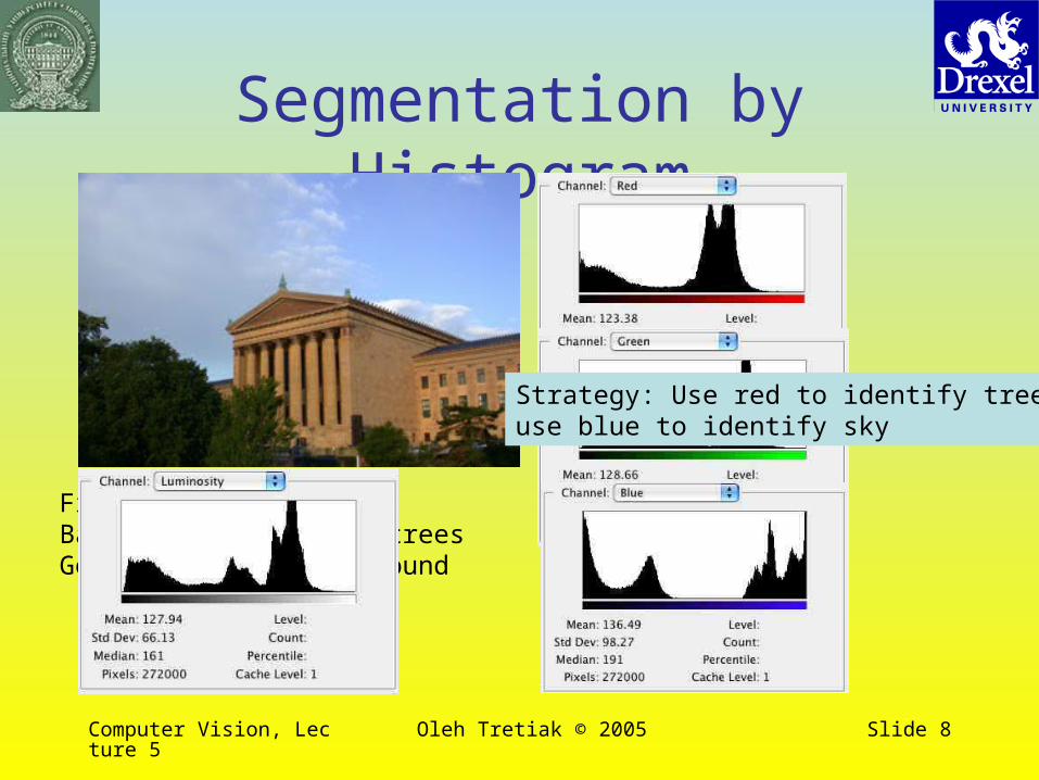
Figure: MuseumBackground: Sky plus treesGoal: Identify background
Segmentation by Histogram
Strategy: Use red to identify trees,use blue to identify sky

Computer Vision, Lecture 5 Oleh Tretiak © 2005 Slide 9
Edit Detection

Computer Vision, Lecture 5 Oleh Tretiak © 2005 Slide 10
Clustering
• Preliminary processing produces binary image
• Identify connected groups of pixels in the image

Computer Vision, Lecture 5 Oleh Tretiak © 2005 Slide 11
Topological Clustering
• Given: Array with values 0 and -1– Cells with 0 are unmarked (background), cells with -1 are marked
(objects)
• Goal: Assign value 1 for all pixels in first object, value 2 in second object, etc.
• Topological principle: If a pixel is in object k, and another pixel is adjacent to it and is marked, then it is also in object k.
0
-1
21
pixel values

Computer Vision, Lecture 5 Oleh Tretiak © 2005 Slide 12
Topological Clustering Algorithm
topological_clusters {k = 1;p = coordinates_of_marked_pixelwhile (p != -1) {
label_connected_pixels( p, k)k = k+1;p = coordinates_of_marked_pixel
}}coordinages_of_marked_pixel {
for i = 1 to last {if val[i] == -1
return i; }
return -1; }
}

Computer Vision, Lecture 5 Oleh Tretiak © 2005 Slide 13
Connected Pixel Labeling
label_connected_pixels( p, k) { // label all marked // pixels connected to p with kval(p) = k;change = 1;while ( change == 1 ) {
change = 0;for i = 1 to last {
if (val[i] == -1) & (pixel_adjacent_to(i) == k) {
val[i] = k;change = 1;
}}
))
pixel i
pixel adjacentto i
Computer Vision, Lecture 5 Oleh Tretiak © 2005 Slide 14
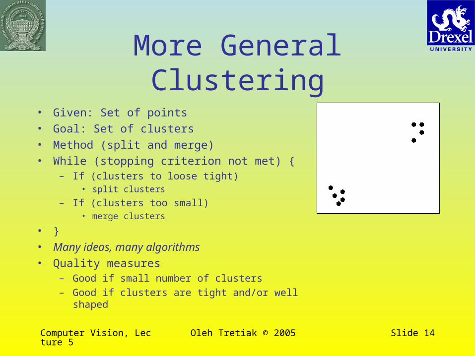
More General Clustering
• Given: Set of points
• Goal: Set of clusters
• Method (split and merge)
• While (stopping criterion not met) {– If (clusters to loose tight)
• split clusters
– If (clusters too small)• merge clusters
• }
• Many ideas, many algorithms
• Quality measures– Good if small number of clusters– Good if clusters are tight and/or well shaped

Computer Vision, Lecture 5 Oleh Tretiak © 2005 Slide 15
Adjacency Matrix MergeScatter
0
2
4
6
8
10
12
14
16
18
20
0 5 10 15 20
1
6
5
4
3
2
7
0.0 3.2 5.4 11.0 11.4 15.7 16.43.2 0.0 7.4 13.9 14.2 18.1 19.65.4 7.4 0.0 7.1 7.2 10.8 14.1
11.0 13.9 7.1 0.0 1.0 5.4 7.711.4 14.2 7.2 1.0 0.0 4.6 8.315.7 18.1 10.8 5.4 4.6 0.0 9.916.4 19.6 14.1 7.7 8.3 9.9 0.0
Adjacency Matrix
1 1_2 1_2_3 1_2_3_4_5_6234 4_5 4_5_6567

Computer Vision, Lecture 5 Oleh Tretiak © 2005 Slide 16
Merge Rules
• Find adjacency matrix d(i, j) = ||pi–pj||
• Merge: – Find smallest d(i, j)– Merge these two clusters. Call new cluster
k– For all l ≠ i, j, d(l, k) = min(d(l, i), d(l, j))

Computer Vision, Lecture 5 Oleh Tretiak © 2005 Slide 17
k – Mean Clustering
• Assign data to k clusters
• Iteratively– Compute ci , means of clusters for i = 1 ... k
– Re-assign data to the cluster associated with the closest mean
Computer Vision, Lecture 5 Oleh Tretiak © 2005 Slide 18
Graph-Based Segmentation
• Split image into parts
• Assign a graph vertex to each part
• Assign edges that measure similarity between parts
• Partition graph into components that are similar within component and different among components.

Computer Vision, Lecture 5 Oleh Tretiak © 2005 Slide 19
Advantages and Disadvantages
• Similarity measures can be chosen for the problem at hand– Similarity according to intensity– Similarity in color– Similarity in texture– Similarity in geometry
• No good method of choosing similarity measures and merging criteria
Computer Vision, Lecture 5 Oleh Tretiak © 2005 Slide 20
Model-Based Segmentation
• Method of segmentation should be chosen on the basis of model of objects being segmented
• We will consider clustering of straight lines from edge detection data

Computer Vision, Lecture 5 Oleh Tretiak © 2005 Slide 21
Hough Transform
• Coordinates of a line on a plane are
• The transform
€
x cosθ + ysinθ = r
€
H (r,θ ) = f (x cosθ − l sinθ ,∫ xsinθ + l cosθ )dl

Computer Vision, Lecture 5 Oleh Tretiak © 2005 Slide 22
Hough Coordinates
x
y
r
q
Image of one point
Hough transform

Computer Vision, Lecture 5 Oleh Tretiak © 2005 Slide 23
Line Detection

Computer Vision, Lecture 5 Oleh Tretiak © 2005 Slide 24
Lines With and Without Noise


