This article was downloaded by: [University of Saskatchewan Library]On: 17 April 2013, At: 16:35Publisher: Taylor & FrancisInforma Ltd Registered in England and Wales Registered Number: 1072954 Registered office: MortimerHouse, 37-41 Mortimer Street, London W1T 3JH, UK

International Journal of Computer MathematicsPublication details, including instructions for authors and subscription information:http://www.tandfonline.com/loi/gcom20

Computing accurate solutions for coupled systemsof second order partial differential equations IILucas jôdar aa Departamento de Matemática Aplicada, Universidad Politécnica de Valencia,Apdo, Valencia, 22.012, SpainVersion of record first published: 19 Mar 2007.

To cite this article: Lucas jôdar (1992): Computing accurate solutions for coupled systems of second order partialdifferential equations II, International Journal of Computer Mathematics, 46:1-2, 63-75

To link to this article: http://dx.doi.org/10.1080/00207169208804139

PLEASE SCROLL DOWN FOR ARTICLE

Full terms and conditions of use: http://www.tandfonline.com/page/terms-and-conditions

This article may be used for research, teaching, and private study purposes. Any substantial orsystematic reproduction, redistribution, reselling, loan, sub-licensing, systematic supply, or distributionin any form to anyone is expressly forbidden.

The publisher does not give any warranty express or implied or make any representation that thecontents will be complete or accurate or up to date. The accuracy of any instructions, formulae, anddrug doses should be independently verified with primary sources. The publisher shall not be liable forany loss, actions, claims, proceedings, demand, or costs or damages whatsoever or howsoever causedarising directly or indirectly in connection with or arising out of the use of this material.

Intern. J Computer Math., Vol. 46, pp. 63-75 Reprints available directly from the publisher Photocopying permitted by license only

0 1992 Gordon and Breach Science Publishers S.A. Printed in the United States of America

COMPUTING ACCURATE SOLUTIONS FOR COUPLED SYSTEMS OF SECOND ORDER PARTIAL DIFFERENTIAL EQUATIONS I1

LUCAS JODAR

Departamento de Matematica Aplicada, Universidad Polit&cnica de Valencia, Apdo 22.012 Valencia, Spain

(Received 24 June 1991; in jna l form 7 October 1991)

In this paper an infinite series solution for solving non homogeneous coupled systems of second order partial differential equations is proposed. Given a finite domain and an admissible error E we construct an analytical approximate solution whose error is uniformly bounded by E in the given domain.

KEY WORDS: Coupled partlal differential system, Initial-boundary value problem, truncation, upper error bound, accuracy, analytical approximate solution.

C.R. CATEGORIES: (3.1.8

1985 AMS(M0S) Subject Classification: 35A20, 35A40, 65N15, 651305.

1 INTRODUCTION

Coupled systems of partial differential equations appear in many physical problems such as in magnetohydrodynamic flows [12], in the study of temperature distribution in a composite heat conductor 131, or in the study of the expected conditional temperature for heat flow in a random two-component laminates [3,7,9].

Methods based on the transformation of a coupled system into a new system of uncoupled equations may be found in [4,13], and its drawbacks have been treated in [ 5 ] .

The aim of this paper is to find analytical approximate solution of coupled systems of the type

where U = (u,, . . . . ,urn)=, F(x) and G(x, t ) are vectors in Rm and A is a matrix in

Dow

nloa

ded

by [

Uni

vers

ity o

f Sa

skat

chew

an L

ibra

ry]

at 1

6:35

17

Apr

il 20

13

RrnX m such that

For each eigenvalue z of A, Re(z) > 0 (1.4)

This paper may be regarded as a continuation of [8] where the case G = 0 has been studied. The paper is organized as follows. In Section 2 an infinite series solution of the problem (l. l t(1.3) is given. Section 3 is concerned with the construction of a finite computable analytical approximate solution of the problem so that the approximation error be smaller than an admissible error E in a prefixed domain D = [O,p] x [to, t,], with to > 0. This construction is performed by truncation of the infinite series and the approximation of certain matrix exponentials by truncation of its Taylor series expansion. An illustrative example showing the availability of the construction of the approximate solutions is given.

For the sake of clarity in the presentation we recall some concepts that will be used in the following. If C is a matrix in R m x m we denote by ICl1 its operator norm defined as the square root of the maximum eigenvalue of CTC where CT is the transpose matrix of C,[11], p. 14.

The set of all eigenvalues of a square matrix C will be denoted by o(C) and the identity matrix in Rm "" is denoted by I. We recall that for a square matrix C and for z E o(C), the index of z is the first positive integer k such that Ker(C - z q , =

Ker(C - zI)~", see [6], p. 556 for details.

2 AN INFINITE SERIES SOLUTION O F THE PROBLEM

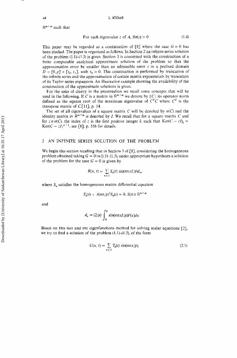
We begin this section recalling that in Section 3 of [a], considering the homogeneous problem obtained taking G = 0 in (l . l t(1.3), under appropriate hypotheses a solution of the problem for the case G = 0 is given by

where Sn satisfies the homogeneous matrix differential equation

and

d,, = (2jp) Sop sin(nnxIjpjp)f(x)dx

Based on this fact and the eigenfunctions method for solving scalar equations [2], we try to find a solution of the problem (l.lH1.3), of the form

Dow

nloa

ded

by [

Uni

vers

ity o

f Sa

skat

chew

an L

ibra

ry]

at 1

6:35

17

Apr

il 20

13

COUPLED SYSTEMS OF P.D.E's 65

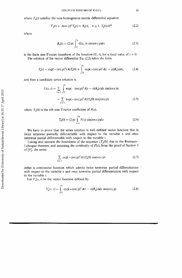
where Tn(t) satisfies the non-homogenous matrix differential equation

To(t) + A(nn,/p)'T,,(t) = B,(t), n 2 1, T,(t)&[Wm (2.2)

where

is the finite sine Fourier transform of the function G(., t), for a fixed value of t > 0. The solution of the vector differential Eq. (2.2) takes the form

and thus a candidate series solution is

where Tn(0) is the nth sine Fourier coefficient of F(x),

We have to prove that the series solution is well defined vector function that is twice termwise partially differentiable with respect to the variable x and onc? termwise partial differentiable with respect to the variable t.

Taking into account the boundness of the sequence {T,(O)} due to the Riemann- Lebesgue theorem, and assuming the continuity of F(x), from the proof of Section 3 of [XI, the series

defies a continuous function which admits twice termwise partial differentiation with respect to the variable x and once termwise partial differentiation with respect to the variable t.

Let Vn(x, t) be the vector function defined by

Dow

nloa

ded

by [

Uni

vers

ity o

f Sa

skat

chew

an L

ibra

ry]

at 1

6:35

17

Apr

il 20

13

Thus the candidate solution U(.u, t ) defined by (2.5) will be a rigorous solution if the series

defines a continuous function which admits termwise partial differentiation twice with respect to .u and once with respect to the variable t.

Note that from (2.8) it follows that

From the derivation theorcm for functional series [ I , Theorem 9.141, the series V(x, t ) dcfilicd by (2.9) is termwise partially differentiable and it defines a continuous function, if for any positive number I, , the following series

and

are uniformly convergent in the domain D(to, 6) = [O,p] x [ to - 6, to + 61, where S is a positive number such that O < 6 i t o .

Let us suppose that the function G(x, t ) appearing in (1.1) is a bounded function for (x , t)&[O, p] x [0, sc[, which admits continuous partial derivatives dG/Jx and i12G/ri.u2 and satisfies

G(0, t ) = G(y, t), for all t > 0 (2.12)

and

dG/a"x, J2G/(ix2 are uniformly bounded in [O, p] x [O, m[ (2.1 3)

then, from [14], p. 71, there exists a constant Q > 0 such that

llBn(t)l I Q/n2, n 2 1 , uniformly for t > 0 (2.14)

Dow

nloa

ded

by [

Uni

vers

ity o

f Sa

skat

chew

an L

ibra

ry]

at 1

6:35

17

Apr

il 20

13

COUPLED SYSTEMS OF P.D.E's 67

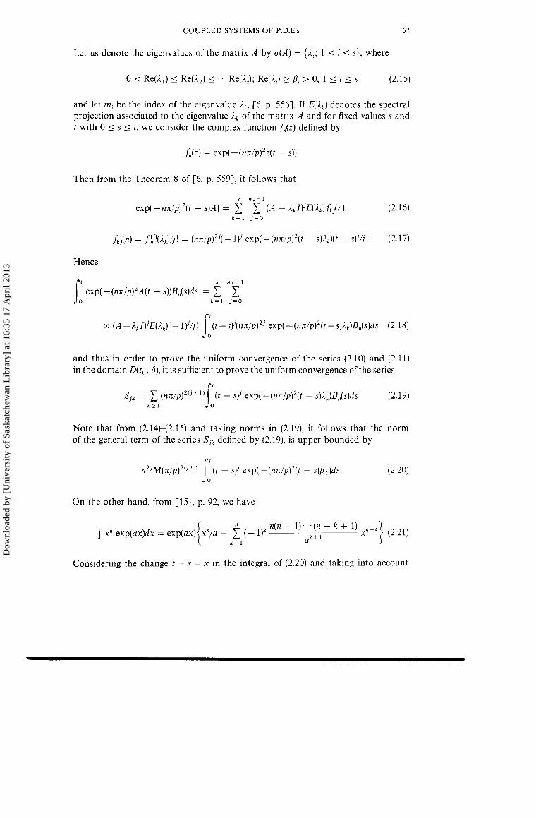
Let us denote the eigenvalues of the matrix A by a(A) = {ii; 1 I i I s), where

and let mi be the index of the eigenvalue i.,, [6, p. 5561. If E(&) denotes the spectral projection associated to the eigenvalue E., of the matrix A and for fixed values s and t with 0 I s < t , we consider the complex function fn(z) defined by

Then from the Theorem 8 of [6, p. 5591, it follows that

Hence

and thus in order to prove the uniform convergence of the series (2.10) and (2.1 1 ) in the domain D(tO, 4, it is sufficient to prove the uniform convergence of the series

Sjk = 1 (nn/p)'(j+') (t - s)j exp(-(nn/p)'(t - s)?.,)B,(s)ds (2.19) n t l

Note that from (2.14n2.15) and taking norms in (2.19), it follows that the norm of the general term of the series Sjk defined by (2.19), is upper bounded by

On the other hand, from [15) , p. 92, we have

Considering the change t - s = x in the integral of (2.20) and taking into account

Dow

nloa

ded

by [

Uni

vers

ity o

f Sa

skat

chew

an L

ibra

ry]

at 1

6:35

17

Apr

il 20

13

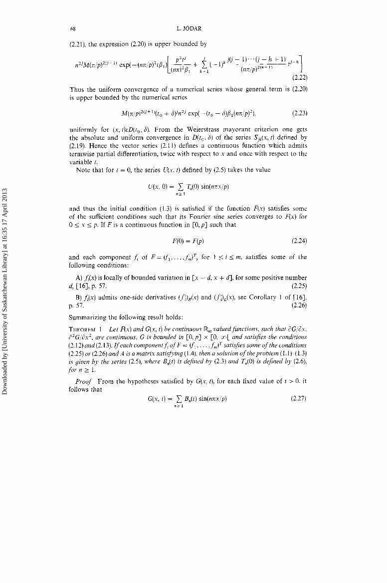
(2.21), the expression (2.20) is upper bounded by

Thus the uniform convergence of a numerical series whose general term is (2.20) is upper bounded by the numerical series

uniformly for (x, t)cD(t0, 6). From the Weierstrass mayorant criterion one gets the absolute and uniform convergence in D(t,, 6) of the series Sj,(x, t ) defined by (2.19). Hence the vector series (2.11) defines a continuous function which admits termwise partial differentiation, twice with respect to .u and once with respect to the variable t.

Note that for t = 0, the series U(x, t ) defined by (2.5) takes the value

and thus the initial condition (1.3) is satisfied if the function F(x) satisfies some of the sufficient conditions such that its Fourier sine series converges to F(x) for 0 I x I p. If F is a continuous function in [O,p] such that

and each component of F = V;, . . . , f,)', for 1 I i _< m, satisfies some of the following conditions:

A) f i (x) is locally of bounded variation in [x - d, x + d l , for some positive number d, [16], p. 57. (2.25)

B) f , (x) admits one-side derivatives (,fi),(x) and (f :),(x), see Corollary 1 of [16], p. 57. (2.26)

Summarizing the following result holds:

THEOREM 1 Let F(x) and G(x , t ) be continuous R, valued functions, such that ?G/dx, c'2G/2x2, are corttinuous, G is bounded in [O,p] x [0, cc [ and satisjies the condifions (2.12) and (2.13). Ifeach componentf, of F = (f,, . . . , f,)' satisjies some of the conditions (2.25) or (2.26) and A is a matrix satisj>ing (1.4), then a solution of the problem ( l . l t ( 1 . 3 ) is given by the series (2.5), where B,(t) is de$ned by (2.3) and Tn(0) is dejined by (2.6), for n 2 1.

Proof From the hypotheses satisfied by G(x, t), for each fixed value of t > 0 , it follows that

G(x, t ) = Bn(t) sin(nnx/p) (2.27) n > 1

Dow

nloa

ded

by [

Uni

vers

ity o

f Sa

skat

chew

an L

ibra

ry]

at 1

6:35

17

Apr

il 20

13

COUPLED SYSTEMS OF P.D.E's 69

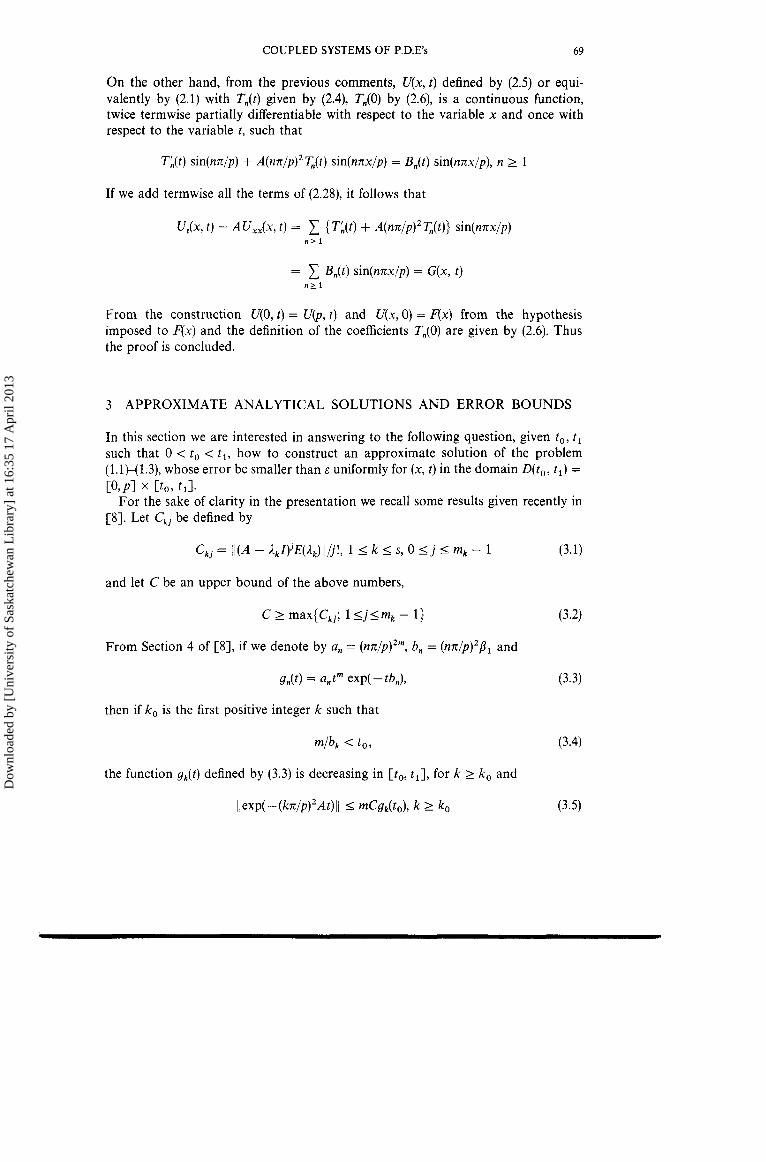
On the other hand, from the previous comments, U(x, t) defined by (2.5) or equi- valently by (2.1) with T,(t) given by (2.4), T,(O) by (2.6), is a continuous function, twice termwise partially differentiable with respect to the variable x and once with respect to the variable t, such that

If we add termwise all the terms of (2.28), it follows that

From the construction U(0, t ) = U(p, t) and U(x, 0) = F(x) from the hypothesis imposed to F(x) and the definition of the coefficients T,(O) are given by (2.6). Thus the proof is concluded.

3 APPROXIMATE ANALYTICAL SOLUTIONS AND ERROR BOUNDS

In this section we are interested in answering to the following question, given to, t , such that 0 < to < t,, how to construct an approximate solution of the problem (1.1)-(1.3), whose error be smaller than E uniformly for (x, t ) in the domain D(t,, t,) =

CO,PI X [to, t l l . For the sake of clarity in the presentation we recall some results given recently in

[8] Let Ckj be defined by

and let C be an upper bound of the above numbers,

From Section 4 of [8], if we denote by a, = (n~ /p )~" , b, = (nn/p)'B, and

then if ko is the first positive integer k such that

the function g,(t) defined by (3.3) is decreasing in [to, t,], for k 2 k, and

Dow

nloa

ded

by [

Uni

vers

ity o

f Sa

skat

chew

an L

ibra

ry]

at 1

6:35

17

Apr

il 20

13

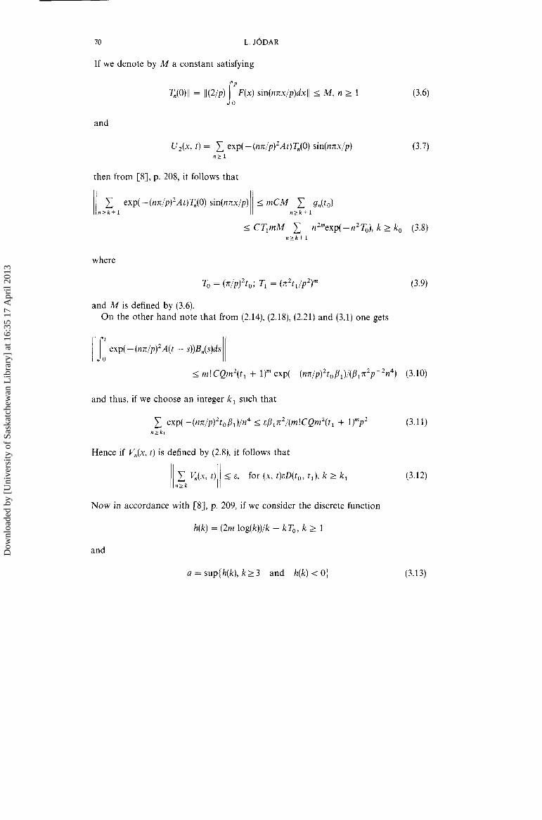
If we denote by M a constant satisfying

and

then from [ 8 ] , p. 208, it follows that

where

and M is defined by (3.6). On the other hand note that from (2.14), (2.18), (2.21) and (3.1) one gets

and thus, if we choose an integer k , such that

Hence if Vn(x, t) is defined by (2.81, it follows that

Now in accordance with 181, p. 209, if we consider the discrete function

and

a = sup{h(k), k 2 3 and h(k) < 0)

Dow

nloa

ded

by [

Uni

vers

ity o

f Sa

skat

chew

an L

ibra

ry]

at 1

6:35

17

Apr

il 20

13

COUPLED SYSTEMS OF P.D.E's 71

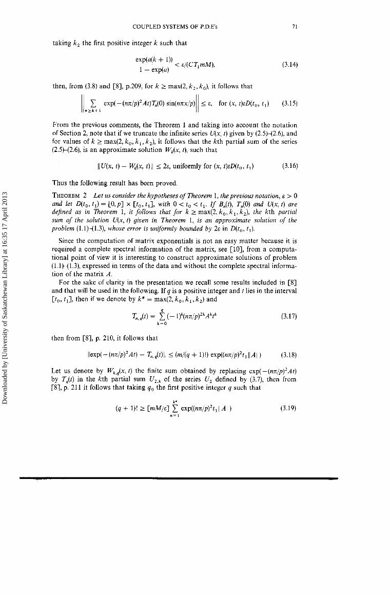
taking k, the first positive integer k such that

then, from (3.8) and [a], p.209, for k 2 max(2, k,, k,), it follows that

exp( - (nn/p)'~t)T,(O) sin(nnx/p) I 6, for (x, t)cD(t,, t ,) (3.15) II.E, I I From the previous comments, the Theorem 1 and taking into account the notation of Section 2, note that if we truncate the infinite series U(x, t) given by (2.5)-(2.6), and for values of k 2 max(2, k,, k,, k,), it follows that the kth partial sum of the series (2.5)-(2.6), is an approximate solution Wk(x, t), such that

I / U(x, t) - Wk(x, t) 1 1 1 2&, uniformly for (x, t)&D(t0, t,) (3.16)

Thus the following result has been proved.

THEOREM 2 Let us consider the hypotheses of Theorem 1, theprevious notation, E > 0 and let D(t,, t,) = [O,p] x [to, t,], with 0 < to < t,. If B,(t), T,,(O) and U(x, t) are defined as in Theorem 1, it follows that for k 2 max(2, k,, k,, k,), the kth partial sum of the solution U(x, t) given in Theorem 1, is an approximate solution of the problem (1.1)-(1.3), whose error is uniformly bounded by 28 in D(t,, t,).

Since the computation of matrix exponentials is not an easy matter because it is required a complete spectral information of the matrix, see [lo], from a computa- tional point of view it is interesting to construct approximate solutions of problem (1.1)-(1.3), expressed in terms of the data and without the complete spectral informa- tion of the matrix A.

For the sake of clarity in the presentation we recall some results included in [a] and that will be used in the following. If q is a positive integer and t lies in the interval [to, t,], then if we denote by k* = max(2, k,, k,, k,) and

then from [a], p. 210, it follows that

Let us denote by Wk,,(x, t) the finite sum obtained by replacing exp(-(nnlp)'At) by T4(t) in the kth partial sum U2,, of the series U2 defined by (3.7), then from [8], p. 211 it follows that taking q, the first positive integer q such that

Dow

nloa

ded

by [

Uni

vers

ity o

f Sa

skat

chew

an L

ibra

ry]

at 1

6:35

17

Apr

il 20

13

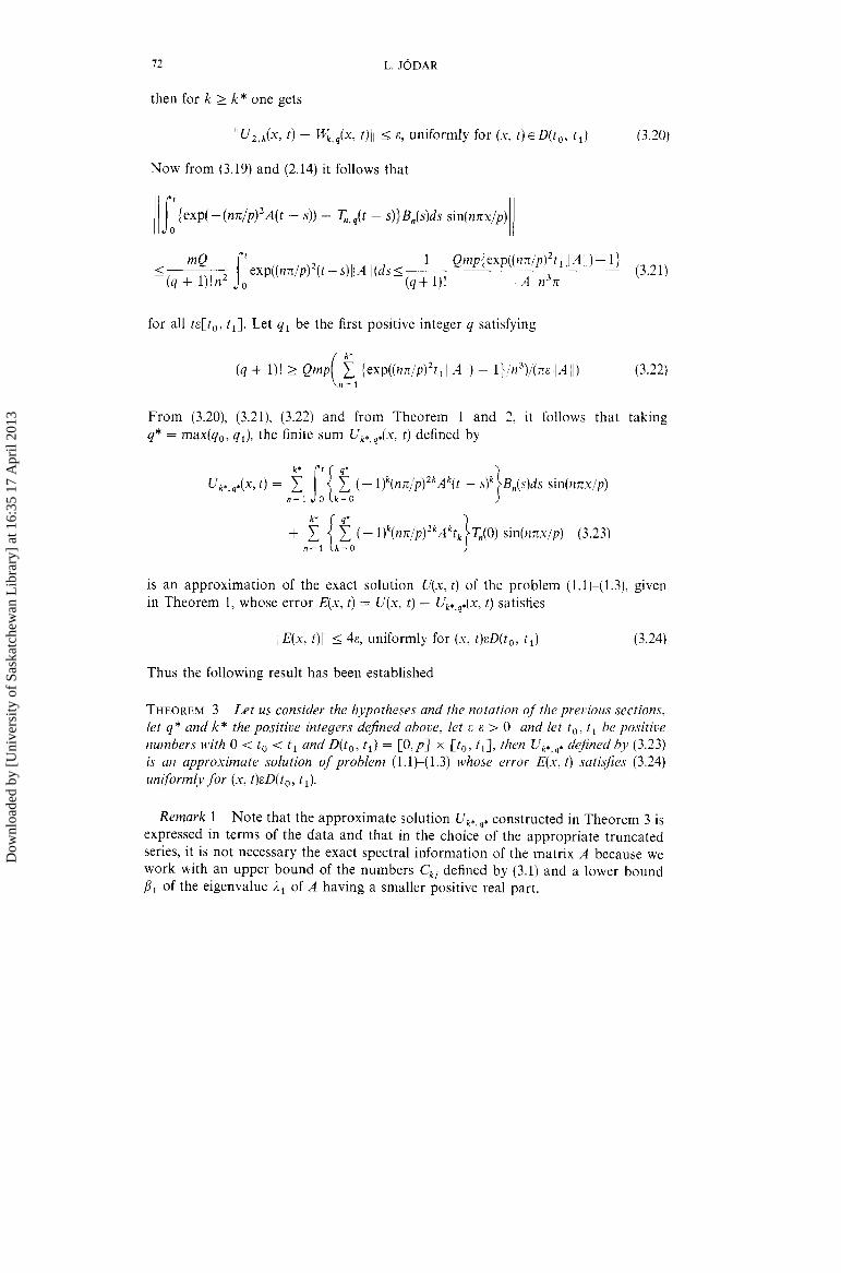
then for k 2 k* one gets

ii U 2 , ,(x, t ) - W,, ,(x, t ) ( 1 I E , uniformly for (x, t ) E D(t,, t , ) (3.20)

Now from (3.19) and (2.14) it follows that

< - mQ 1 Q m ~ h p ( ( n . r r i ~ ) ~ t , !I Ail) - 1 ) e ~ p ( ( n n / p ) ~ ( t - s) j A (ds I - - (3.21)

(4+ 111 Aln3n

for all t s[ to , t l ] . Let q , be the first positive integer q satisfying

k*

(q + I ) ! t Qmp( Z { e ~ p ( ( n n / p ) ~ t , A ! ) - 1 ) l n 3 ) / ( n a A ) (3.22) \ I t - 1

From (3.20), (3.21), (3.22) and from Theorem 1 and 2, it follows that taking q* = max(q,, q,), the finite sum U ,,,,, (.u, t ) defined by

is an approximation of the exact solution U(x, t ) of the problem (1.1)-(1.3), given in Theorem 1 , whose error E(x, t ) = U ( x , t ) - Uk,,,,(x, t ) satisfies

/ E(x, t)I 1 4 ~ , uniformly for ( x , t )~D( t , , t l ) (3.24)

Thus the following result has been established

THEOREM 3 Let us consider the hypotheses and the notation oj'the precious sections, let q* and k* the positive integers defined above, let s E > 0 and let t o , t , be positive numbers with 0 < t , < t , and D(t,, t , ) = [0, p] x [ to , f , I , then U,,,,, dejined by (3.23) is an approximate solution of problem ( l . l t ( 1 . 3 ) whose error E(x, t ) satisjes (3.24) uniformly for (x, t)~D(t,, , t l ) .

Remark 1 Note that the approximate solution U,,,,, constructed in Theorem 3 is expressed in terms of the data and that in the choice of the appropriate truncated series, it is not necessary the exact spectral information of the matrix A because we work with an upper bound of the numbers Ckj defined by (3.1) and a lower bound p, of the eigenvalue i, of A having a smaller positive real part.

Dow

nloa

ded

by [

Uni

vers

ity o

f Sa

skat

chew

an L

ibra

ry]

at 1

6:35

17

Apr

il 20

13

COUPLED SYSTEMS OF P.D.E's 73

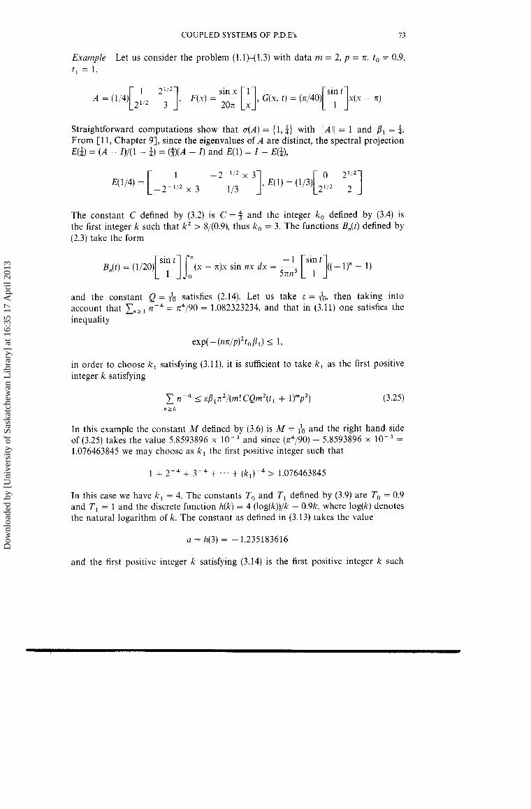
Example Let us consider the problem (1.1)-(1.3) with data m = 2, p = n . to = 0.9, t , = 1,

Straightforward computations show that o ( A ) = ( 1 , $1 with IIAil = 1 and B, = $. From [ l l , Chapter 91, since the eigenvalues of A are distinct, the spectral projection E($) = ( A - 1)/(1 - $1 = ($)(A - I ) and E ( l ) = I - E($),

The constant C defined by (3.2) is C = $ and the integer k , defined by (3.4) is the first integer k such that k 2 > 8/(0.9), thus k , = 3. The functions Bn(t) defined by (2.3) take the form

~ ~ ( t ) = ( I / ~ o ) [ ~ ~ : '1 I:(, - z ) x sin n x d x = ----j 5nn - [Siy [I(( - 1). - 1)

and the constant Q = satisfies (2.14). Let us take E = &, then taking into account that x,,, = n4/90 = 1.082323234, and that in (3.11) one satisfies the inequality

in order to choose k , satisfying (3.11), it is sufficient to take k , as the first positive integer k satisfying

In this example the constant M defined by (3.6) is M = and the right hand side of (3.25) takes the value 5.8593896 x and since (n4/90) - 5.8593896 x =

1.076463845 we may choose as k , the first positive integer such that

In this case we have k, = 4. The constants To and T, defined by (3.9) are T o = 0.9 and T , = 1 and the discrete function h (k ) = 4 ( log(k)) /k - 0.9k, where log(k) denotes the natural logarithm of k . The constant as defined in (3.13) takes the value

and the first positive integer k satisfying (3.14) is the first positive integer k such

Dow

nloa

ded

by [

Uni

vers

ity o

f Sa

skat

chew

an L

ibra

ry]

at 1

6:35

17

Apr

il 20

13

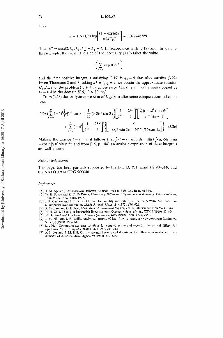
that

k + 1 > ( l /a ) log

Thus k* = max(2, k,, k , , k2) = k , = 4. In accordance with (3.19) and the data of this example, the right hand side of the inequality (3.19) takes the value

and the first positive integer q satisfying (3.19) is qo = 9 that also satisfies (3.22). From Theorems 2 and 3, taking k* = 4, q = 9, we obtain the approximate solution U4,,(x, t ) of the problem (l . lH1.3), whose error E(x, t ) is uniformly upper bound by 4.5 = 0.4 in the domain C0.9, 11 x [0, a[.

From (3.23) the analytic expression of U4,,(x, t ) after some computations takes the form

9 2lI2 t - s ) ~ sin s ds (2/5n) Z ( - ~)*{(i)~* sin x + 1 ( 3 / 2 ) " sin 3 ~ } [ ~ ~ , ~ ] [Ib( k = o 27 - t k+ l/(k + 1 ) 1

9 2'12 k 0

+ k = o ' (-r)k[2'12 3 ] {[-(8/3) sin 2x - (4ki2/15) sin 4x 11 (3.26)

Making the change t - s = u, it follows that f,(t - s ) ~ sin s ds = sin t So uk cos u du -cos t So uk sin u du, and from [15, p. 1841 an analytic expression of these integrals are well known.

Acknowledgements

This paper has been partially supported by the D.G.I.C.Y.T. grant PS 90-0140 and the NATO grant CRG 900040.

References

[I] T. M. Apostol, Mathematical Analysis, Addison-Wesley Pub. Co., Reading MA. [2] W. E. Boyce and R. C. Di Prima, Elementary Dlfferential Equations and Boundary Value Problems,

John-Wiley, New York, 1977. [3] J. R. Cannon and R. E. Klein, O n the observability and stability of the temperature distribution in

a composite heat conductor, SIAM J. Appl. Math., 24 (1973), 59G602. [4] R. Courant and D. Hilbert, Methods of Mathematical Physics, Vol. 11, Interscience, New York, 1962. 151 H. H. Chiu, Theory of irreducible linear systems, Quarterly Appl. Maths., XXVII (1969), 87-104. [6] N. Dunford and J. Schwartz, Linear Operators I, Interscience, New York, 1957. 173 J. M. Hill and J. R. Willis, Analytical aspects of heat flow in random two-component laminates,

XLVI(2) (1988), 353-364. [8] L. Jodar, Computing accurate solutions for coupled systems of second order partial differential

equations, Int. J. Computer Maths., 37 (1990), 201-212. [9] A. I. Lee and J. M. Hill, O n the general linear coupled systems for diffusion in media with two

diffusivities, J. Math. Anal. Appls., 89 (1982), 53G538.

Dow

nloa

ded

by [

Uni

vers

ity o

f Sa

skat

chew

an L

ibra

ry]

at 1

6:35

17

Apr

il 20

13

COUPLED SYSTEMS O F P.D.E's 75

[lo] C. B. Moler and C. F. Van Loan, Nineteen dubious ways to compute the exponential of a matrix, SIAM Review 20 (1978), 801-836.

[ I t ] J. M. Ortega and W. C. Rheinboldt, Iterative Solution of Nonlinear Equations in Seueral Variables, Academic Press, New York, 1970.

[I21 M. Sezgin, Magnetohydrodynamic flow in a rectangular duct, Int. J. Numer. Method.7 Fluids, 7 (1987), 697-718.

[I31 E. C. Zachmanoglou and D. W. Thoe, Introduction to Partial Dlfferential Equations with Applications, William and Wilkins, Baltimore, 1976.

[14] A. Zygmund, Trigonometric Series, Second ed., Vols. I and 11, Cambridge Univ. Press, 1977. [I51 I. S. Gradshteyn and I. M. Ryzhik, Tables of Integrals, Series, and Products, Academic Press, New

York, 1980. [I61 R. V. Churchill and J. W. Brown, Fourier Series and Boundary Value Problems, McGraw-Hill,

London, 1978. [17] P. Lancaster and M. Tismenetsky, The Theory ofMatrices, Academic Press, New York, 2nd ed., 1985.

Dow

nloa

ded

by [

Uni

vers

ity o

f Sa

skat

chew

an L

ibra

ry]

at 1

6:35

17

Apr

il 20

13