K e y w o r d s - - Radial basis functions, Eigenvalues, Numerical methods, Laplacian, corner singu- larities.
1. I N T R O D U C T I O N
Many positive properties of radial basis function (RBF) methods have been identified in con- nection with boundary-value problems (BVPs) [1-4]. They are grid-free numerical schemes very suitable for problems in irregular geometries. They can exploit accurate and smooth representa- l~ions of the boundary, are very easy to implement, and can be spectrally accurate [5,6]. It would ]be expected tha t the benefits experienced by the use of RBFs in BVPs would carry over for eigenvalue problems. In this article, we formulate and apply an RBF-based method to compute eigenmodes of elliptic operators.
Given a linear elliptic second-order partial differential operator L and a bounded region ~ in :~n with boundary 0~, we seek eigenpairs (Au) E (C, C(gt)) satisfying
Lu + Au = O, in ~, and
L s u = 0, on O~t, (1)
*Supported by NSF Grant DMS-0104229.
0898-1221/04/$ - see front matter ~) 2004 Elsevier Ltd. All rights reserved. doi:10.1016/j.camwa.2003.08.007
Typeset by A2~S-TEX
562 R.B. PLATTE AND T. A. DRISCOLL
where L s is a linear boundary operator of the form
L B u = a u + b(n. Vu). (2 )
Here, a and b are given constants and n is the unit outward normal vector defined on the boundary. We assume that gt is open and that the eigenvalue problem is well-posed.
We use an interpolating RBF approximation of an eigenfunction of (1) and replace the eigen- value problem above with a finite-dimensional eigenvalue problem. In order to compute the eigenpairs of the modified system, we approximate the operator L by a matrix that incorporates the boundary conditions and then use standard techniques to find the eigenvalues and eigenvec- tors of this matrix.
As pointed out in [2,7], straightforward RBF approximations are relatively inaccurate near the boundaries, and special attention should be given to this issue. We study the boundary clustering of nodes and the collocation of the PDE on the boundary and verify that they are effective techniques for preventing degradation of the solution near the edges of the domain.
We consider the effect of corner singularities in 2-D regions. It is known that some eigenfunc- tions are not smooth at corners with interior angle 7r/~ where ~ is not integer. As a result, a straightforward RBF approximation is severely degraded in this case. Several authors have exploited explicit information about the singular behavior of an eigenfunction at a corner to propose efficient algorithms to compute eigenvalue for these regions (see, for example, [8-10]). With these efforts as motivation, we append terms to the RBF expansion that approximate the singular behavior of an eigenfunction. To our knowledge, this type of singular augmentation has not been used before with RBFs.
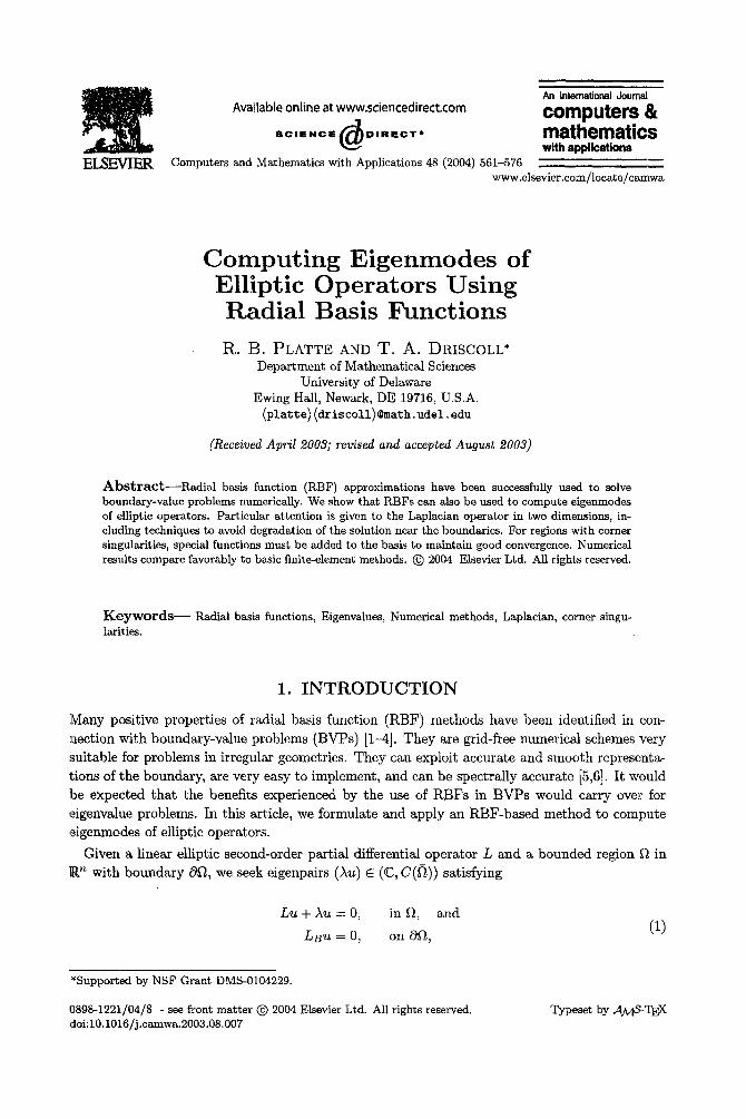
The remainder of this article is organized as follows. In the next section, we introduce RBF approximations. In Section 3, we formulate the problem in matrix form. In Section 4, we present the boundary treatment techniques. In Section 5, a scheme for regions with corner singularities is introduced. We carry out several experiments in 2-D regions for the Laplacian operator for a disk, an L-shaped region, and a rhombus as pictured in Figure 1, and compare to finite elements and pseudospectral methods.
(a) (b) (c)
Figure 1. 2-D regions considered for the numerical experiments.
2. R A D I A L B A S I S F U N C T I O N S
Let g {Y~}~=I be a finite set of distinct points in ~n. Given a function ¢ from ~+ to ~, we write the standard RBF approximation of a function u:
N
- ( l l x - y l12), x e (3 ) i= l
The points Yi are called centers and ¢ the radial basis function [11]. The coefficients c~ are chosen so that h satisfies certain interpolation criteria to be discussed later.
Computing Eigenmodes 563
Several choices for ¢ have been presented in the literature [7,11,12]. Some of the most commonly used RBFs are
¢ ( r ) = r ~,
¢(r) = r 2 log(r),
¢(~) = (1 - r )~p(r ) ,
¢(r) = exp ( - ( ~ ) ~ ) ,
¢(r) = V ~ + r~,
(cubic),
(thin plate sphne),
(Wendland functions [13], where p is polynomial),
(Gaussian),
(multiquadric),
where r is real and nonnegative and c is a positive constant. The multiquaclric, in particular, has been successfully used to solve elliptic problems numerically [2,4]. It was introduced by Hardy [14], and Kansa [1] applied it to solve PDEs in the early 1990s.
In order to determine the coefficients ai, a set of N distinct interpolation points in ~ is needed. Usually, the same set of points is used for centers and interpolation. Taking centers outside the domain appropriately, however, has been shown to be an effective way of improving accuracy near tim boundary--see, e.g., [2,7]. If u(xj) , j = 1 ,2 , . . . , N, were known, finding the ai would require solution of an g × N linear system Ac~ = u, A - : [¢(llxi -YjH2)]N×~, a --- [ a l , a2 , . . . ,aN] T, and u --- [u(xl ) ,u(x2) , . . . ,u(xg)] T. A is called the RBF interpolation matrix and, for some R.BFs, is positive definite [11].
3. A L G O R I T H M
There are different ways to use (3) to derive a finite-dimensional eigenvalue problem. We s:hall start with the method we find the most efficient. The idea behind this scheme is to approximate the operator L by a matrix L¢ that also incorporates the boundary conditions.
For NI nodes in the interior of the domain and NB nodes on the boundary, N = NI + NB, NI X N we denote the interpolation points by {x~}i=l E ~2 and { i}~=N~+l E Ofl. In order to obtain L¢,
we enforce the boundary condition at every point x~ on the boundary, and evaluate the RBF approximation (3) at the interior interpolation points to obtain
~--~ iLB¢ (llxj - Y~H2) =0, j - - - N I + I , N I + 2 , . . . , N . i=0
In the notation LB¢(Ilxj -Y~II2), it is understood that LB is applied to the first variable, then evaluated. This can be written in matrix form as
oN~×I ' (4)
where fil _~ [~(xl), ~2(x2),..., 2~(XNx)] T, Op×q iS the p x q zero matrix,
For the Dirichlet boundary condition, the matrix ..4 becomes the usual RBF interpolation matrix. For the interior points, we also have that
N
~--~ a ,L¢ (llXy - Y~I[2) = Xa (x~), j --- 1 ,2 , . . . ,N/ , i=1
564 R . B . PLATTE AND T, A. DRISCOLL
which can be expressed as Llot = Aft I, (5)
where
i I --- [L¢ ([Ix, - YJ[[2)]NIxN"
Combining (4) and (5), we obtain Left ~ = Aft( (6)
L¢ is the N I x Ns matrix given by
ON e x N t J "
Here, Iv× v is the identity matrix of order p. The RBF approximation of the eigenpairs of (1) is now obtained by computing the eigenvalues
and eigenvectors of the matrix L¢. In some instances, it is necessary or useful to add functions to the RBF approximation (3),
N M
~(x) -= E a~¢ ([Ix - y~ 112) + E fl~g/(x), x e R ~. (7) i : 1 i = 1
To make this system uniquely solvable, it is usually required that N
,gj(x) = 0, j = 1,2, . . . ,M. i~-I
For the Neumann problem, augmentation by a constant is especially appropriate due to the trivial zero mode.
Repeating the procedure above for (7), one obtains the following expression for the operator of the finite-dimensional system
L¢==.L~`421[ INz×Nz ], L O(NB +M) x NI
where
L I =-[L x [Lgj (xi)]g~×M],
[ A r [gj (x,)]Nx×M ] .,42 - [nsgj (XNI+,) ]N~ × M | "
[[gi(xj)]MxN OMxM J A few remarks should be made about the method.
• The matrix .4 (or `42) usually becomes ill-conditioned as the number of nodes increases. This is a common problem when RBFs of global support are used [15].
• For the Dirichlet problem, the matrix ,4 has been proved to be invertible for most RBFs, and conditions that guarantee that `42 is nonsingular are known--see, e.g., [16,17]. For b # 0, there is no proof that these matrices are invertible for any choice of nodes. We point out, however, that for all numerical experiments we performed, the matrices were nonsingular.
• The eigenvalue system is of size Nz, the number of interior nodes, although as an inter- mediate step, one must invert a matrix of size N, the total number of nodes.
• One could rewrite the matrix eigenvalue system using the "inverse RBF operator". In this case, one would seek the eigenpairs (v,fi I) of the matrix He,
The approximate eigenvalues and eigenvectors of (1) would then be 1/v and fiz respec- tively.
Computing Eigenmodes 565
Another approach is to write the finite-dimensional problem as a generalized eigenvalue prob- lem. The idea is to substitute the RBF approximation (3) into the eigenvalue problem (1), leading to the following system:
A I
In. this case, one would seek the generalized eigenvalues and eigenvectors of these matrices. This system is of size N, not NI, but unlike L¢, does not require a matrix inversion. Notice that, in principle, the accuracy of the approximation does not depend on how the eigenpairs of the finite- dimensional problem are computed, but on the RBF and the set of nodes used. The generalized eigenvalue problem also suffers from ill-conditioning.
3.,1. N u m e r i c a l Resu l t s
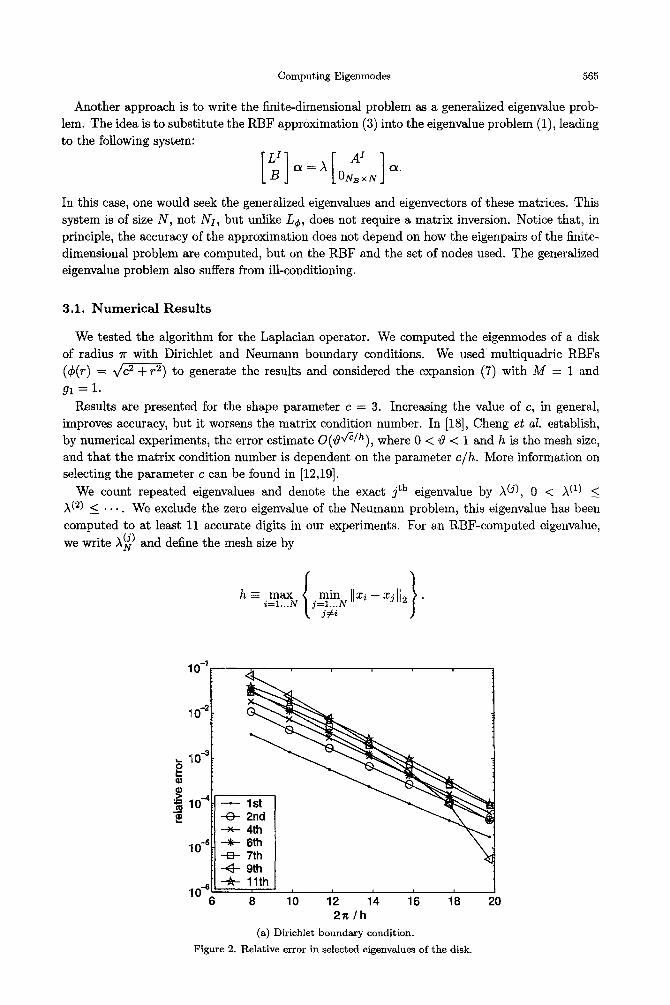
We tested the algorithm for the Laplacian operator. We computed the eigenmodes of a disk of radius lr with Dirichlet and Neumann boundary conditions. We used multiquadric RBFs (¢(r) = V ~ + r 2) to generate the results and considered the expansion (7) with M = 1 and gl =I.
Results are presented for the shape parameter c = 3. Increasing the value of c, in general, iraproves accuracy, but it worsens the matrix condition number. In [18], Cheng et aL establish, by numerical experiments, the error estimate O09v'-~/h), where 0 < d < 1 and h is the mesh size, and that the matrix condition number is dependent on the parameter c/h. More information on selecting the parameter c can be found in [12,19].
We count repeated eigenvalues and denote the exact jth eigenvalue by AO) 0 < A (1) < A (2) <_ -- . . We exclude the zero eigenvalue of the Neumann problem, this eigenvalue has been computed to at least 11 accurate digits in our experiments. For an RBF-computed eigenvalue, we write A(~) and define the mesh size by
/rain llx,-xjll }.
10 -1 10-2} "~ "-e- 2nd ~..-.,,. "~
--x-- 4th " ~ lo-sL] ,~,, 6th \ fl 7th
~ 9th 1 lth
10% 8 1'0 1'2 1'4 16 1'8 21¢/h
(a) Dirichlet boundary condition. Figure 2. Relative error in selected eigenvalues of the disk.
20
566 R.B. PLATTE AND T. A. DRISCOLL
10 -1
10 -3
lo'
10 -5 6
0 X
[]
J - , , , , ,
3rd ~ "~ 5th \
8th ~ / " lOth 12th
I I
10 I'P 14 1'6 18 20 2 ~ / h
(b) Neumann boundary condition.
Figure 2. (cont.)
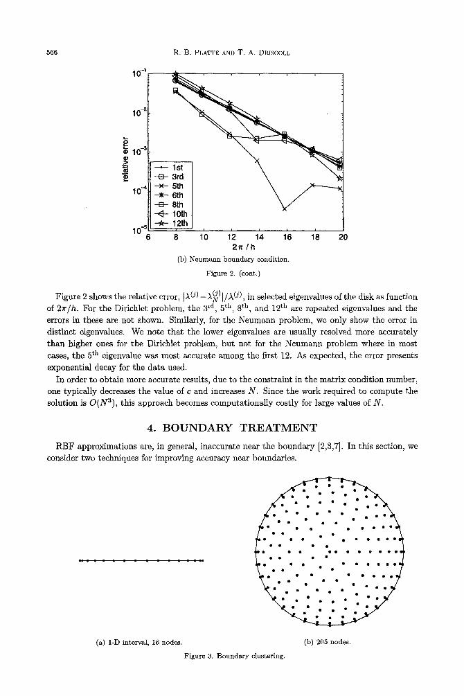
Figure 2 shows the relative error, [A(J)-A(~)]/A(j), in selected eigenvalues of the disk as function of 2~r/h. For the Dirichlet problem, the 3 rd, 5 th, 8 th, and 12 th are repeated eigenvalues and the
errors in these are not shown. Similarly, for the Neumann problem, we only show the error in distinct eigenvalues. We note that the lower eigenvalues are usually resolved more accurately than higher ones for the Dirichlet problem, but not for the Neumann problem where in most cases, the 5 th eigenvalue was most accurate among the first 12. As expected, the error presents exponential decay for the data used.
In order to obtain more accurate results, due to the constraint in the matrix condition number, one typically decreases the value of c and increases N. Since the work required to compute the solution is O(N3), this approach becomes computationally costly for large values of N.
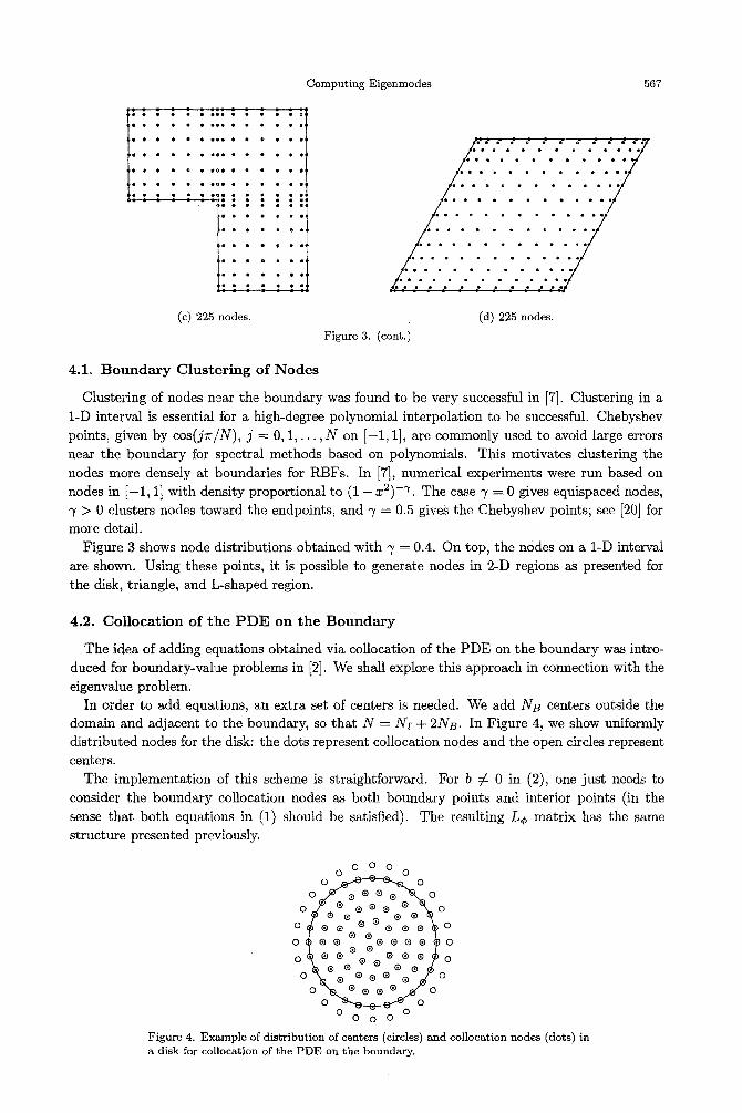
4 . B O U N D A R Y T R E A T M E N T
RBF approximations are, in general, inaccurate near the boundary [2,3,7]. In this section, we consider two techniques for improving accuracy near boundaries.
(a) 1-D interval, 16 nodes.
Figure 3. Boundary clustering.
(b) 205 nodes.
Computing Eigenmodes
iiiiiiii: . . . . . . .
(e) 225 nodes.
567
Figure 3. (cont.)
(d) 225 nodes.
4.1. Boundary Clustering of Nodes
Clustering of nodes near the boundary was found to be very successful in [7]. Clustering in a 1-D interval is essential for a high-degree polynomial interpolation to be successful. Chebyshev points, given by cos(jn/N), j -~ O, 1 , . . . , N on [-1, 1], are commonly used to avoid large errors near the boundary for spectral methods based on polynomials. This motivates clustering the nodes more densely at boundaries for RBFs. In [7], numerical experiments were run based on nodes in [-1, 1] with density proportional to (1 - x2) -7. The case ~ = 0 gives equispaeed nodes, ~/> 0 clusters nodes toward the endpoints, and ~ = 0.5 gives the Chebyshev points; see [20] for more detail.
Figure 3 shows node distributions obtained with ~f -- 0.4. On top, the nodes on a 1-D interval are shown. Using these points, it is possible to generate nodes in 2-D regions as presented for the disk, triangle, and L-shaped region.
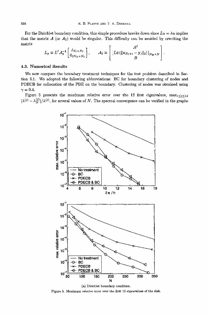
4.2. Co l loca t ion of t he P D E on t he B o u n d a r y
The idea of adding equations obtained via collocation of the PDE on the boundary was intro- duced for boundary-value problems in [2]. We shall explore this approach in connection with the eigenvalue problem.
In order to add equations, an extra set of centers is needed. We add NB centers outside the domain and adjacent to the boundary, so that N = Nr + 2NB. In Figure 4, we show uniformly distributed nodes for the disk: the dots represent collocation nodes and the open circles represent centers.
The implementation of this scheme is straightforward. For b ~ 0 in (2), one just needs to consider the boundary collocation nodes as both boundary points and interior points (in the sense that both equations in (1) should be satisfied). The resulting L¢ matrix has the same structure presented previously.
O O O
000 0 0 0 0 ~ 0 0 ~ 0 0 0 0 0 0 0 0 0
0 0 000 Figure 4. Example of distribution of centers (circles) and collocation nodes (dots) in a disk for collocation of the PDE on the boundary.
568 R.B. PLATTE AND T. A. DRISCOLL
For the Dirichlet boundary condition, this simple procedure breaks down since Lu - - Au implies that the matrix A (or ,42) would be singular. This difficulty can be avoided by rewriting the matrix
L¢- LZA~I [ IN,xN, ] L0=NB xNx J '
4.3. N u m e r i c a l R e s u l t s
[ A, ] A3- [L¢(IIXNI+i--YjII2)]NBxN •
B
We now compare the boundary treatment techniques for the test problem described in Sec- tion 3.1. We adopted the following abbreviations: BC for boundary clustering of nodes and PDECB for collocation of the PDE on the boundary. Clustering of nodes was obtained using
= 0.4. Figure 5 presents the maximum relative error over the 12 first eigenvalues, maxl<j<_12
IA (D - A(~ ) I/A (D , for several values of N. The spectral convergence can be verified in the graphs
L -
£ (9 >=
E
1 0 - 1 ~
10 4
10 4
10-6
10 -7 4 14 16 18
..... Notm~ment -E~BC --x-PDECB - ~ - - P D E C B & B C
6 8 10 12 2 ~ / h
1 0 -1
10 -2
10 -a
.~_ 10 "4
10 ~
10 -7 50 100 150 200 250 300 350
N (a) Dirichlet boundary condition.
Figure 5. Maximum relative error over the first 12 eigenvalues of the disk.
569
10 -1
100
0111 L.,
--x-- PDECB PDECB & BC
10 --s ~ ~ 4 6 8 10 12 14 16 18
2 ~ / h
10 -2
10 ~
1o-' ID
E
10 -7 50 16o 3so
N (b) Neumann boundary condition.
Figure 5. (cont.)
Computing Eigenmodes
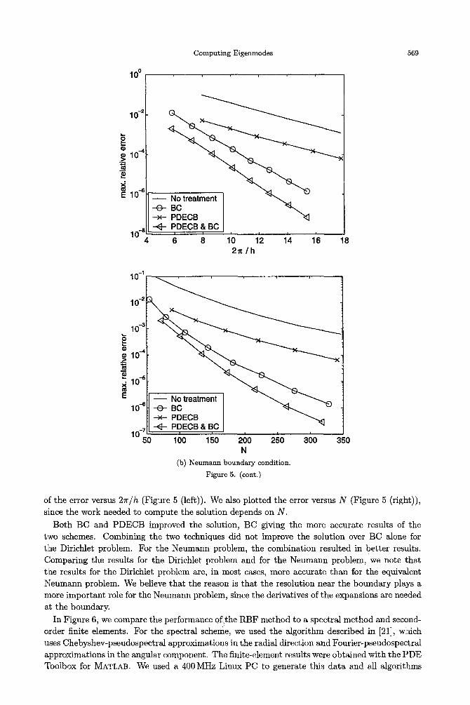
of the error versus 27r/h (Figure 5 (left)). We also plotted the error versus N (Figure 5 (right)), since the work needed to compute the solution depends on N.
Both BC and PDECB improved the solution, BC giving the more accurate results of the two schemes. Combining the two techniques did not improve the solution over BC alone for t]he Dirichlet problem. For the Neumann problem, the combination resulted in better results. Comparing the results for the Dirichlet problem and for the Neumann problem, we note that t:he results for the Dirichlet problem are, in most cases, more accurate than for the equivalent Neumann problem. We believe that the reason is that the resolution near the boundary plays a more important role for the Neumann problem, since the derivatives of the expansions are needed at the boundary.
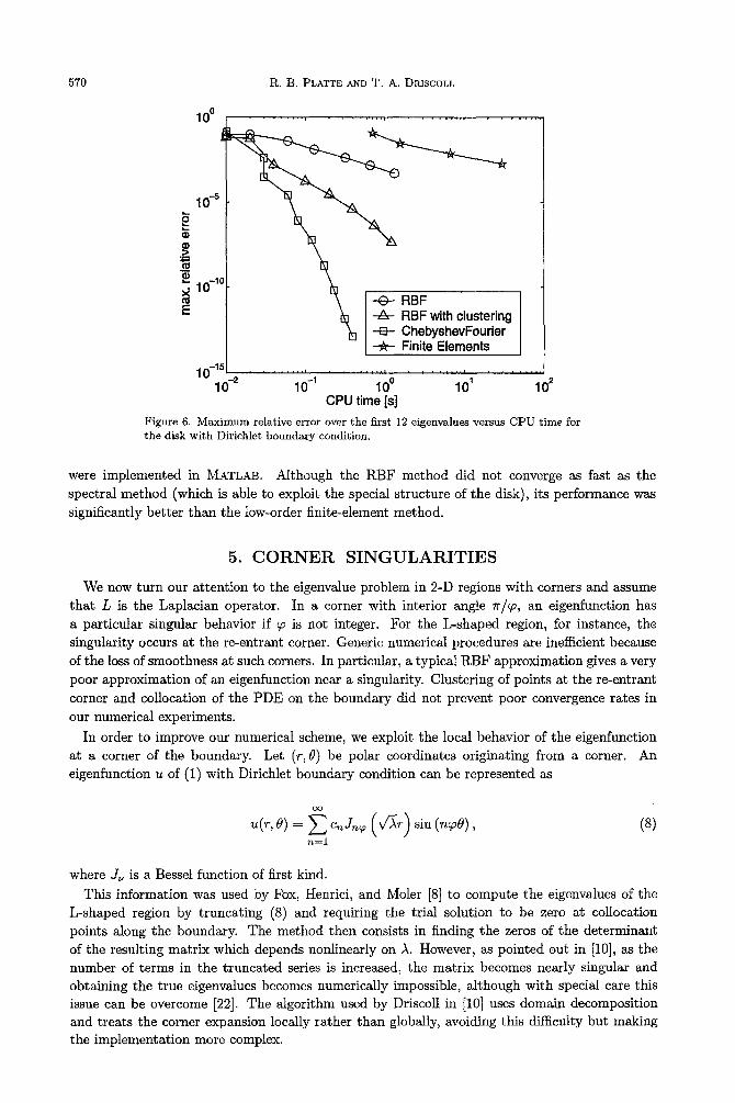
In Figure 6, we compare the performance of)the RBF method to a spectral method and second- order finite elements. For the spectral scheme, we used the algorithm described in [21], which uses Chebyshev-pseudospectral approximations in the radial direction and Fourier-pseudospectral approximations in the angular component. The finite-element results were obtained with the PDE Toolbox for MATLAB. We used a 400 MHz Linux PC to generate this data and all algorithms
Figure 6. Maximum relative error over the first 12 eigenvalues versus CPU time for the disk with Dirichlet boundary condition.
were implemented in MATLAB. Although the RBF method did not converge as fast as the spectral method (which is able to exploit the special structure of the disk), its performance was significantly better than the low-order finite-element method.
5. C O R N E R S I N G U L A R I T I E S
We now turn our attention to the eigenvalue problem in 2-D regions with corners and assume that L is the Laplacian operator. In a corner with interior angle 7r/~, an eigenfunction has a particular singular behavior if ~ is not integer. For the L-shaped region, for instance, the singularity occurs at the re-entrant corner. Generic numerical procedures are inefficient because of the loss of smoothness at such corners. In particular, a typical RBF approximation gives a very poor approximation of an eigenfunction near a singularity. Clustering of points at the re-entrant corner and collocation of the PDE on the boundary did not prevent poor convergence rates in our numerical experiments.
In order to improve our numerical scheme, we exploit the local behavior of the eigenfunction at a corner of the boundary. Let (r, 0) be polar coordinates originating from a corner. An eigenfunction u of (1) with Dirichlet boundary condition can be represented as
oo
u(r,O) = ~-~ c~J ,~ ( V ~ r ) s i n (n~0), (8) r t= l
where Y~ is a Bessel function of first kind.
This information was used by Fox, Henrici, and Moler [8] to compute the eigenvalues of the L-shaped region by truncating (8) and requiring the trial solution to be zero at collocation points along the boundary. The method then consists in finding the zeros of the determinant of the resulting matrix which depends nonlinearly on )~. However, as pointed out in [10], as the number of terms in the truncated series is increased, the matrix becomes nearly singular and obtaining the true eigenvahies becomes numerically impossible, although with special care this issue can be overcome [22]. The algorithm used by Driscoll in [10] uses domain decomposition and treats the corner expansion locally rather than globally, avoiding this difficulty but making the implementation more complex.
Computing Eigenmodes 571
The modification in the RBF-method we propose here is easy to implement and yet avoids degradation of the solution at singular corners. We consider the ascending series
( 1 ) v ~ (_(1/4)z : )k &(z) = z k t r ( . + k + ~)'
k=0
so we have that (8) becomes
u(r, O) = E b~krn~+2k sin(n~O), n = l k=0
where the coefficients bnk are independent of r and 0. Motivated by the last expansion, we add terms of the form r ~v+2k sin(n~0) to the RBF ap-
proximation, i.e., in (7), we let gi = r ~+2k sin(n~0), where n and k are chosen appropriately so that the smallest powers of r are used. We believe that these extra terms help to capture the singular behavior of an eigenfunction at a corner. For the Neumann problem, we have that
u(r, O) = E b~kr~+2k cos(n~0), n=O k=0
which suggests a similar modification. We note that, in our numerical experiments, the matrix A2 obtained with the augmentation
above was nonsingular and that ill-conditioned formulations may arise if the number of singular terms is large compared to the number of collocation nodes.
We believe that a similar singular term augmentation could be applied to RBF approximations of singular boundary value problems and problems in which the nature of the boundary condition changes abruptly, when the expansion of the singular part of the solution is known a priori [23].
5.1. N u m e r i c a l R e s u l t s
We considered two regions with corner singularities in our numerical experiments: the L-shaped region of vertices (0, zr/2), (lr/2, Tr/2), (zr/2, 0), (% 0), (zr, 7r), and (0, zr), and the rhombus with supplementary angles 60 ° and 120 ° and sides of length ~r. We also used multiquadric RBFs to generate the results, with c = 0.6 for the L-shaped region and c = 1.2 for the rhombus.
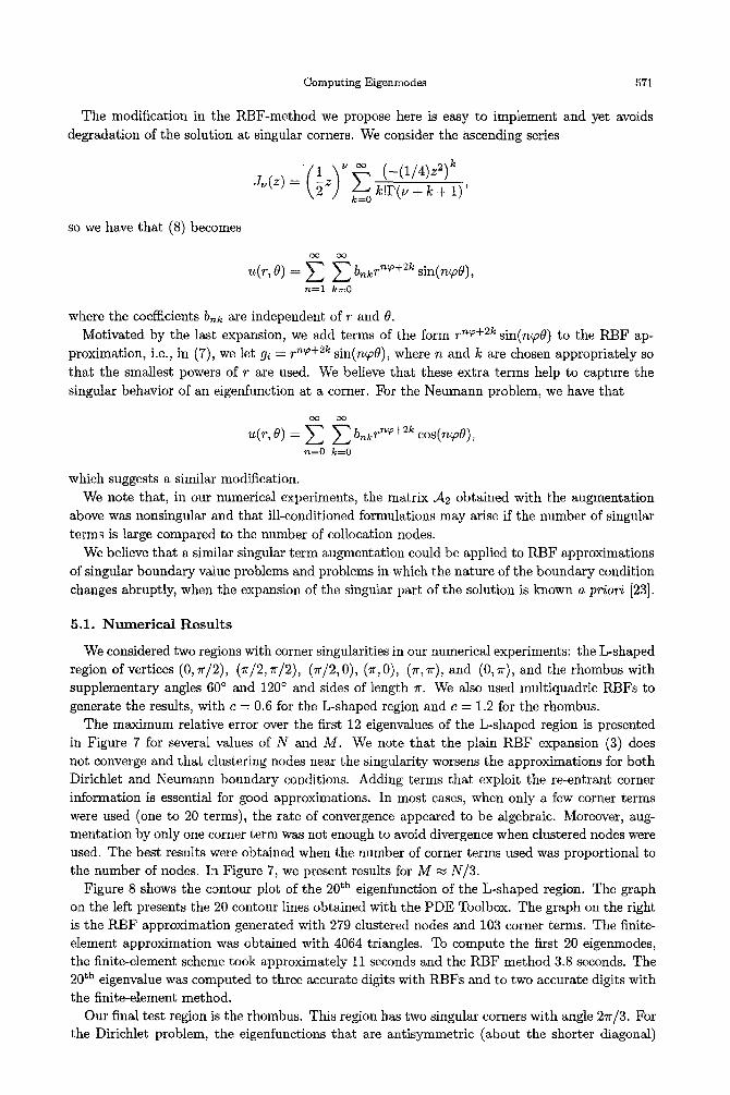
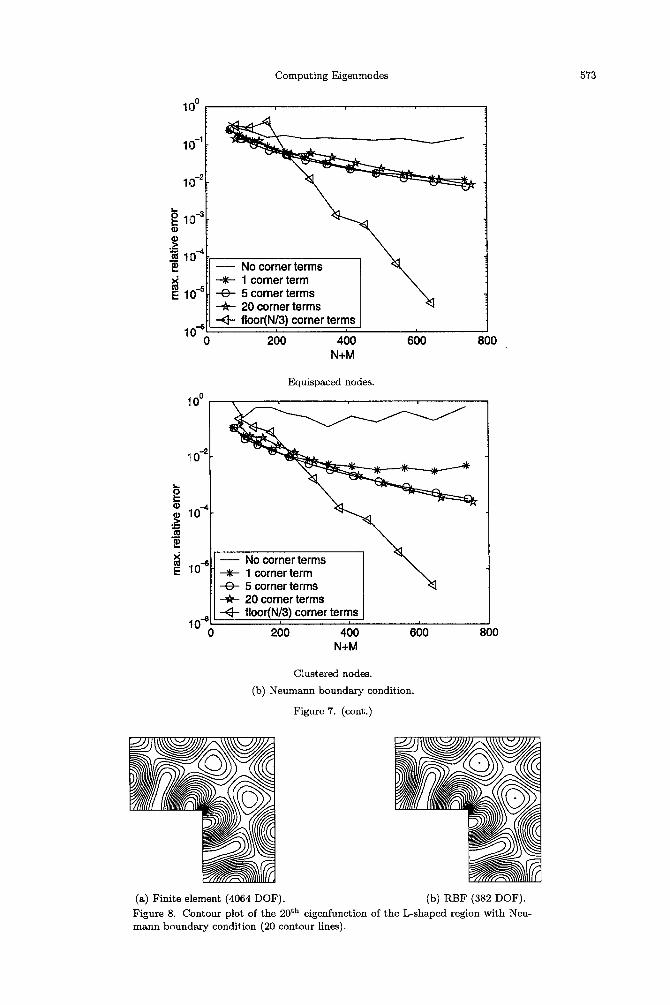
The maximum relative error over the first 12 eigenvalues of the L-shaped region is presented in Figure 7 for several values of N and M. We note that the plain RBF expansion (3) does not converge and that clustering nodes near the singularity worsens the approximations for both Dirichlet and Neumann boundary conditions. Adding terms that exploit the re-entrant corner information is essential for good approximations. In most cases, when only a few corner terms were used (one to 20 terms), the rate of convergence appeared to be algebraic. Moreover, aug- mentation by only one corner term was not enough to avoid divergence when clustered nodes were used. The best results were obtained when the number of corner terms used was proportional to the number of nodes. In Figure 7, we present results for M ~ N/3.
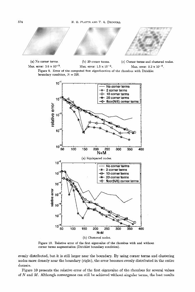
Figure 8 shows the contour plot of the 20 th eigenfunction of the L-shaped region. The graph on the left presents the 20 contour lines obtained with the PDE Toolbox. The graph on the right is the RBF approximation generated with 279 clustered nodes and 103 corner terms. The finite- element approximation was obtained with 4064 triangles. To compute the first 20 eigenmodes, the finite-element scheme took approximately 11 seconds and the RBF method 3.8 seconds. The 20 ta eigenvalue was computed to three accurate digits with RBFs and to two accurate digits with the finite-element method.
Our final test region is the rhombus. This region has two singular corners with angle 2~r/3. For the Dirichlet problem, the eigenfunctions that are antisymmetric (about the shorter diagonal)
572 R.B. PLATTE AND T. A. DRISCOLL
are smooth since they are const ructed using the modes of a equi la teral t r iangle [24]. Other eigen-
functions present s ingular behavior, as i t is the case of the first mode. Al though this s ingular i ty
is not as s t rong as i t is in a re-entrant corner, i t sti l l results in poor convergence rates for global
methods t ha t use smooth functions to approx imate the solution. In fact, in [6], an algebraic
convergence ra te is predic ted when RBFs are used to in terpola te such modes. Our results show
tha t this behavior can be avoided by singular corner augmenta t ion .
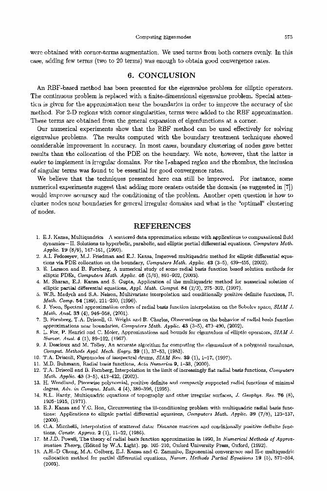
F igure 9 shows the error in the first eigenfunction of the rhombus. The errors presented range
from 0 (white) to the max imum absolute error (black) indica ted below each plot. One can see
tha t the error is larger a t the singular corners if the s t anda rd R B F expansion is used (left).
When corner te rms are added (center), the error decreases in magni tude and becomes more
(a) Finite element (4064 DOF). (b) RBF (382 DOF). Figure 8. Contour plot of the 20 th eigenfunction of the L-shaped region with Neu- mann boundary condition (20 contour lines).
574 R . B . PLATTE AND W. A. Df~ISCOLL
(a) No corner terms. (b) 20 corner terms. (c) Corner terms and clustered nodes.
Max. error: 2.6 x 10 -3 . Max. error: 1.5 x 10 -4. Max. error: 9.2 x 10 -6. Figure 9. Error of the computed first eigenfunction of the rhombus with Dirichlet boundary condition, N = 225.
1 0 -1 ~ ~
No corner terms 2 corner terms
- ~ - 10 corner terms 10-z -,A,- 20 corner terms
.~ 10 -~
10 .4
l O - S ~ 50 100 150 200 250 300 350 400
N+M (a) Equispaced nodes.
10-2 - - No corner terms I ~ 2 corner terms
10-~ I - e - 10 corner terms I ~ 20 corner terms
10 .4 [ - ~ - floor(N/6) corner terms
~ 1 0 -5 >=
10 -6
10 -~'
to-~ 50 1 O0 150 200 250 300 350 400
N+M
(b) Clustered nodes.
Figure 10. Relative error of the first eigenvMue of the rhombus with and without corner terms augmentation (Dirichlet boundary condition).
even ly d i s t r ibu ted , b u t i t is st i l l larger near t he boundary . By us ing corner t e r m s and c lus te r ing
nodes more dense ly near t h e b o u n d a r y (r ight) , t h e e r ror becomes even ly d i s t r i b u t e d in t h e ent i re
domain .
F i g u r e 10 presents t h e re la t ive e r ror of t he first e igenvalue of t h e r h o m b u s for several va lues
of N and M . A l t h o u g h convergence can stil l be achieved w i t h o u t s ingular t e rms , t h e bes t resul ts
Computing Eigenmodes 575
were obtained with corner-terms augmentation. We used terms from both corners evenly. In this ca.,se, adding few terms (two to 20 terms) was enough to obtain good convergence rates.
6. C O N C L U S I O N
An RBF-based method has been presented for the eigenvalue problem for elliptic operators. The continuous problem is replaced with a finite-dimensional eigenvalue problem. Special atten- tion is given for the approximation near the boundaries in order to improve the accuracy of the method. For 2-D regions with corner singularities, terms were added to the RBF approximation. These terms are obtained from the general expansion of eigenfunctions at a corner.
Our numerical experiments show that the RBF method can be used effectively for solving eigenvalue problems. The results computed with the boundary treatment techniques showed considerable improvement in accuracy. In most cases, boundary clustering of nodes gave better results than the collocation of the PDE on the boundary. We note, however, that the latter is easier to implement in irregular domains. For the L-shaped region and the rhombus, the inclusion of singular terms was found to be essential for good convergence rates.
We believe that the techniques presented here can still be improved. For instance, some numerical experiments suggest that adding more centers outside the domain (as suggested in [7]) would improve accuracy and the conditioning of the problem. Another open question is how to cluster nodes near boundaries for general irregular domains and what is the "optimal" clustering of nodes.
R E F E R E N C E S 1. E.J. Kansa, Multiquadrics--A scattered data approximation scheme with applications to computational fluid
dynamics--II. Solutions to hyperbolic, parabolic, and elliptic partial differential equations, Computers Math. Applie. 19 (8/9), 147-161, (1990).
2. A.I. Fedoseyev, M.J. Friedman and E.J. Kansa, Improved multiquadric method for elliptic differential equa- tions via PDE collocation on the boundary, Computers Math. Applic. 43 (3-5), 439-455, (2002).
;~. E. Larsson and B. Fornberg, A numerical study of some radial basis function based solution methods for elliptic PDEs, Computers Math. Applic. 46 (5/6), 891-902, (2003).
4. M. Sharan, E.J. Kansa and S. Gupta, Application of the multiquadric method for numerical solution of elliptic partial differential equations, Appl. Math. Comput. 84 (2/3), 275-302, (1997).
5. W.R. Madych and S.A. Nelson, Multivariate interpolation and conditionally positive definite functions, II, Math. Comp. 54 (189), 211-230, (1990).
6. J. Yoon: Spectral approximation orders of radial basis function interpolation on the Sobolev space, SIAM J. Math. Anal. 33 (4), 946-958, (2001).
7. B. Fornberg, T.A. Driscoll, G. Wright and R. Charles, Observations on the behavior of radial basis function approximations near boundaries, Computers Math. Applie. 43 (3-5), 473-490, (2002).
8. L. Fox, P. Henrici and C. Moler, Approximations and bounds for eigenvalues of elliptic operators, SIAM J. Numer. Anal. 4 (1), 89-102, (1967).
9. J. Descloux and M. Tolley, An accurate algorithm for computing the eigenvalues of a polygonal membrane, Comput. Methods Appl. Mech. Engrg. 39 (1), 37-53, (1983).
10. T.A. Driscoll, Eigenmodes of isospectral drums, SIAM Rev. 39 (1), 1-17, (1997). 1].. M.D. Buhmann, Radial basis functions, Acta Numerica 9, 1-38, (2000). 12. T.A. Driscoll and B. Fornberg, Interpolation in the limit of increasingly flat radial basis functions, Computers
Math. Applie. 43 (3-5), 413-422, (2002). 13. H. Wendland, Piecewise polynomial, positive definite and compactly supported radial functions of minimal
degree, Adv. in Comput. Math. 4 (4), 389-396, (1995). 14. R.L. Hardy, Multiquadric equations of topography and other irregular surfaces, J. Geophys. Res. 76 (8),
1905-1915, (1971). 15. E.J. Kansa and Y.C. Hon, Circumventing the ill-conditioning problem with multiquadric radial basis func-
17. M.J.D. Powell, The theory of radial basis function approximation in 1990, In Numerical Methods of Approx- imation Theory, (Edited by W.A. Light). pp. 105-210, Oxford University Press, Oxford, (1992).
18. A.H.-D Cheng, M.A. Golberg, E.J. Kansa and G. Zammito, Exponential convergence and H-c multiquadric collocation method for partial differential equations, Numer. Methods Partial Equations 19 (5), 571-594, (2003).
576 R.B. PLATTE AND T. A. DRISCOLL
19. S. Rippa, An algorithm for selecting a good value for the parameter e in radial basis function interpolation, Adv. Comp. Math. 11 (2/3), 193-210, (1999).
20. B. Fornberg, A Practical Guide to Pseudospectral Methods, Cambridge University Press, (1996). 21. L.N. Trefethen, Spectral Methods in MATLAB, SIAM, Philadelphia, PA, (2000). 22. T. Betcke and L.N. Trefethen, Private communications, (2003). 23. Z. Yosibash, Numerical analysis on singular solutions of the Poisson equation in two-dimensions, Comput.
Mech. 20 (4), 320-330. 24. B.J. McCartin, Eigenstructure of the equilateral triangle, Part I: The Dirichlet problem, SIAM Rev. 45 (2),