Computing spectra with an Eckart frame to refineand test a methane potential

Xiao-Gang Wang and Tucker Carrington

Chemistry DepartmentQueen’s University

16 juin 2015

1 / 61

Calculating spectra is useful because it enablesspectroscopists to

verify the accuracy of or refine potential energy surfaces

predict the position (and intensity) of unobserved transitions

assign observed spectra

2 / 61

Perturbation Theory

Spectroscopists often use a zeroth-order harmonic model andperturbation theory

For low-lying levels of semi-rigid molecules it works pretty well.

Methane vibrational levels in the Octad (∼ 4000 cm−1 abovethe ZPE) computed with fourth and sixth order perturbationtheory differ by about 8 cm−1.

Most ab initio programs use second order perturbation theory.

Nearly degenerate levels cause perturbation theory to breakdown.

The density of states increases with energy.

3 / 61

For

high-lying states

molecules in which coupling and anharmonicity are important

one, instead, needs numerically accurate solutions to theSchroedinger equation

Hψn = Enψn

4 / 61

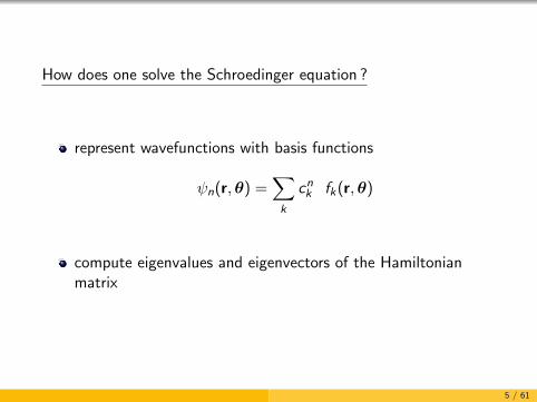
How does one solve the Schroedinger equation ?

represent wavefunctions with basis functions

ψn(r,θ) =∑

k

cnk fk(r,θ)

compute eigenvalues and eigenvectors of the Hamiltonianmatrix

5 / 61

Fundamental Recipe

K + V → Hbasis−−−→ H→ eigenvalues,

eigenvectors→ energies,

wavefunctions

→ Spectrum

6 / 61

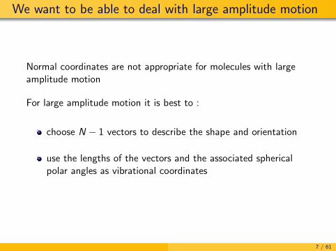
We want to be able to deal with large amplitude motion

Normal coordinates are not appropriate for molecules with largeamplitude motion

For large amplitude motion it is best to :

choose N − 1 vectors to describe the shape and orientation

use the lengths of the vectors and the associated sphericalpolar angles as vibrational coordinates

7 / 61

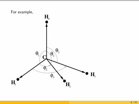
For example,

H

H

H

θθ

φ

φ

θ

H

C

3

1

0

3

1

2

3

2

2

8 / 61

Consider first the J = 0 problem

The general KEO is

T = Ts + Tb

with

Ts = −N−2∑k=0

1

2µk

∂2

∂r2k

and

Tb = Tb,diag + Tb,off .

9 / 61

Tb,diag = [B0(r0) + B1(r1)]

[− 1

sin θ1

∂

∂θ1sin θ1

∂

∂θ1+

1

sin2 θ1L2z

]

+N−2∑k=2

[B0(r0) + Bk(rk)] l2k

+B0(r0)

2L2z + 2N−2∑

k 6=k′=2

lkz lk′z

Tb,off = B0(r0)

(L+)a−1 + (L−)a+1 +N−2∑

k 6=k′=2

(lk+lk′− + lk−lk′+)

10 / 61

A convenient basis is

fk1,l1,k2,l2,m2··· = χk1(r1)Θm1l1

(θ1)χk2(r2)Θm2l2

(θ2)Φm2(φ2) · · ·

with m1 = −m2 −m3 − · · ·

In this basis

there are simple equations for all KEO matrix elements

singularities in the KEO cause no trouble.

11 / 61

Between 10 and 100 1-d functions required for each coordinate.

⇒ > 103N−6 multi-d basis functions required.

The Hamiltonian matrix is

too large to calculate

too large to store in memory

too large to diagonalise

12 / 61

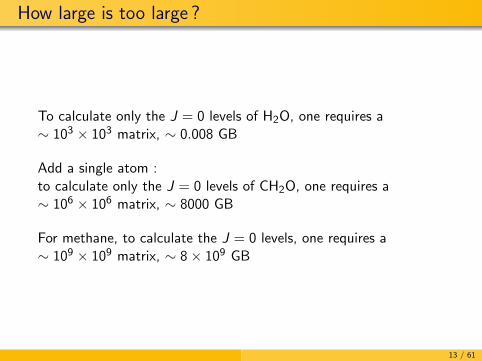
How large is too large ?

To calculate only the J = 0 levels of H2O, one requires a∼ 103 × 103 matrix, ∼ 0.008 GB

Add a single atom :to calculate only the J = 0 levels of CH2O, one requires a∼ 106 × 106 matrix, ∼ 8000 GB

For methane, to calculate the J = 0 levels, one requires a∼ 109 × 109 matrix, ∼ 8× 109 GB

13 / 61

Lanczos Algorithm

H =

· · · · · ·· · · · · ·· · · · · ·· · · · · ·· · · · · ·· · · · · ·

→· · 0 0· · · 00 · · ·0 0 · ·

= T

Among the eigenvalues of T are eigenvalues of H

Eigenvectors of H are obtained from those of T

14 / 61

Limitations of a product basis

Even for J = 0 methane, a product basis calculation is large

|α0 α1 α2 α3〉|l1 l2m2 l3m3 〉

It would be necessary to use ∼ 209 basis functions (4000 GB forone vector) !

15 / 61

Contracted basis functions

It is better to use products of eigenfunctions of reduced-dimensionHamiltonians.

E.g.,

H = Hbend + Hstretch + ∆coupling

Hbend b(θθθ) = Eb b(θθθ)

Hstretch s(rrr) = Es s(rrr)

s(rrr)b(θθθ) is a contracted basis function.

A small number of the s(rrr)b(θθθ) are retained.

16 / 61

Basis lmax = mmax nbend E cutb nb ni nstretch E cut

s ns nfinal

Basis I 25 3.26M 8090 280 10 5049 20000 260 72800∗ 1 M = 1 million. ni is the number of PODVR basis functions for ri with i = 0, 1, 2, 3.

33× 109 → 72× 103

reduction of six orders of magnitude

17 / 61

Ro-vibrational spectrum of methane

Methane is important

A greenhouse gas

Determining the chemical composition and physical conditionsof atmospheres of Jupiter, Saturn, Uranus, Neptune, Titan,etc

Modelling brown dwarfs

18 / 61

III

FEATURES METHANE IN TITAN’S ATMOSPHERE

This conception of Titan mainly comes form theobservations and measurements made by spacecraftlike Voyager 1 in 1980 and, essentially by the Cassini-Huygens mission (NASA/ESA/ASI) which, since July2004, has revolutionized our knowledge of Saturn’s sys-tem including Titan. One of its main features was theEuropeanHuygens probe descent in Titan’s atmosphereand its landing on the surface on January 14, 2005 aftera two and a half hour descent.TheCassini orbiter conti-nues to regularly flyby Titan and the other kronian

satellites with a host of different instruments (cameras,spectrometers, radar,…), supplementing observationsmade from Earth orbit (Hubble Space Telescope, ISOsatellite) or from the ground, often at higher spectralresolution.A series of large and regularly spaced absorption bandsdue tomethane dominate the Titan spectra recorded bythe DISR (Descent Imager/Spectral Radiometer) of theHuygens probe during its descent, and byVIMS (Visualand Infrared Mapping Spectrometer) on the orbiter.Images taken during the Huygens descent combinedwith radar images from the Cassini orbiter providevaluable information. Fluvial networks cover around1 % of the surface (see Figure 1). Large smooth areas,interpreted as methane and ethane lakes or seas, coverimportant parts of the polar regions.Furthermore, methane decomposition in the upperatmosphere leads to a series of chemical reactions pro-ducing various organic compounds such as ethane(C2H6) and other more complex hydrocarbons. Nitro-gen (N2) dissociation and its recombination withmethane leads to the formation of nitriles like hydrogencyanide (HCN). Polymerization of some compoundsproduces a complex material, which constitutes thesolid particles of the orange haze that fills the atmos-phere. These particles become condensation cores forethane and other gases and continuously fall on Titan’s

�FIG.1:“Dried”

methane

rivers imaged

by theHuygens

probeduring

itsdescent

onTitan.

©NASA/JPL/

SpaceScience

Institute.

�FIG.2:Methane’s

spectrum

complexity.

Horizontal lines

representvibra-

tionenergy

levels.Theblack

curvegives the

numberof

vibrational

sublevels for

eachpolyad.

Thenamescor-

respond to

thedifferent

absorption

bands.Different

spectral regions

are illustrated

by imagesand

spectra: inpink,

a simulated

spectrumfor

lowerpolyads

and, in red, an

exampleof

the spectra

recordedon

Titanby the

Huygensprobe.

©NASA/JPL/

SpaceScience

Institute).

19 / 61

J > 0

If the molecule-fixed axes are attached to two vectors the KEO isstill compact :

T = Ts + Tbr + Tcor

withTbr = Tbr,diag + Tbr,off .

20 / 61

Tbr,diag = [B0(r0) + B1(r1)]

[− 1

sin θ1

∂

∂θ1sin θ1

∂

∂θ1+

1

sin2 θ1(Jz − Lz )2

]

+N−2∑k=2

[B0(r0) + Bk (rk )] l2k

+B0(r0)

J2 − 2(Jz − Lz )2 − 2Jz (Lz ) + 2N−2∑

k 6=k′=2

lkz lk′z

Tbr,off = B0(r0)

(L+)a−1 + (L−)a+1 +N−2∑

k 6=k′=2

(lk+lk′− + lk−lk′+)

Tcor = −B0(r0)

[J−(a+1 + L+) + J+(a−1 + L−)

]

21 / 61

For example,

H

H

H

θθ

φ

φ

θ

H

C

3

1

0

3

1

2

3

2

2

22 / 61

J > 0 basis

fk1,l1,k2,l2,m2··· ,J,K ,M =χk1(r1)Θm1l1

(θ1)χk2(r2)Θm2l2

(θ2)Φm2(φ2) · · ·× DJ∗

MK (α, β, γ)

with m1 = K −m2 −m3 − · · ·

23 / 61

With m1 = K −m2 −m3 − · · ·

all matrix elements of the KEO are known in closed form

singularities in the KEO cause no trouble

24 / 61

However, the basis is a factor of 2J + 1 larger than the alreadyhuge product vibrational basis !

25 / 61

An obvious strategy is to use a basis of products of DJ∗MK

and vibrational eigenfunctions

The Hamiltonian may be written

H = Hvib + Hrv .

The basis is |v〉 DJ∗MK .

Eigenfunctions of Hvib, |v〉, are, in turn, computed in a s(rrr)b(θθθ)basis.

The b(θθθ) are computed in a basis of products of angular functions.

I am using nested contractions.

26 / 61

Two problems

Matrix elements in the |v〉 basis are straightforward if |v〉 (i.e.b(θθθ)) is known in the basis in which the KEO matrix is simple(m1 = K −m2 −m3 − · · · ), however, this requiresrecomputing |v〉 many times, for each K

In the two-vector embedded KEO, coupling between rotationand vibration can be so large that the DJ∗

MK |v〉 basis is too big

27 / 61

A K -independent bend basis

We use m1 = −m2 −m3 − · · ·

rather than m1 = K −m2 −m3 − · · ·

28 / 61

Some of the matrix elements required to compute |v〉 inthis basis may be infinite

For example, those involving the factor

〈Θm2l1| 1

sin2 θ1|Θm2

l ′1〉 ,

are infinite if m2 = 0,

θ1 is the angle between ~r0 and ~r1.

As long as all wavefunctions are tiny near θ1 = 0, πthe infinite integrals cause no trouble

29 / 61

Ro-vibrational coupling is too strong

Although the contracted basis is much smaller,

the size of the contracted bend-stretch basis

required for J > 5 is too big.

30 / 61

For many molecules, ro-vibrational coupling is smaller inan Eckart frame.

The orientation of a frame with the z axis along a bond does notchange when a bond is stretched.

θHHz

x

(α, β

, γ )

O

1

21

H

θHz

x

(α, β

, γ )

O

1

1

2

31 / 61

The orientation of an Eckart frame does change when a bond isstretched

θHH

z

x

(α, β, γ )

O

1

21H

θH

z

x

(α, β, γ )

O

1

1

2

32 / 61

It is straightforward to use an Eckart frame with normalcoordinates.

How does one use an Eckart frame with polyspherical coordinates ?

The best of both worlds : vibrational coordinatesthat enable one to deal with large-amplitudemotion AND an Eckart frame that minimizesro-vibrational coupling

33 / 61

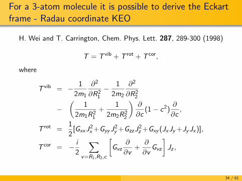
For a 3-atom molecule it is possible to derive the Eckartframe - Radau coordinate KEO

H. Wei and T. Carrington, Chem. Phys. Lett. 287, 289-300 (1998)

T = T vib + T rot + T cor,

where

T vib = − 1

2m1

∂2

∂R21

− 1

2m2

∂2

∂R22

−(

1

2m1R21

+1

2m2R22

)∂

∂c(1− c2)

∂

∂c,

T rot =1

2[GxxJ

2x +GyyJ

2y +GzzJ

2z +Gxy (JxJy +JyJx )],

T cor = − i

2

∑v=R1,R2,c

[Gvz

∂

∂v+

∂

∂vGvz

]Jz ,

34 / 61

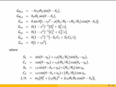
GR1z = −ΛερR2 sin(θ − θe),

GR2z = ΛρR1 sin(θ − θe),

Gcz = Λ sin θ[1−ερ2−ρ(R1/R2−εR2/R1) cos(θ−θe)],

Gxx = Λ(1− c2)−1[S21 + S2

2/ε],

Gyy = Λ(1− c2)−1[C 21 + C 2

2 /ε],

Gxy = Λ(1− c2)−1[−S1C1 + S2C2/ε],

Gzz = Λ[1 + ερ2],

where

S1 = sin(θ−ηe) + ερ(R2/R1) sin(θe−ηe),

C1 = cos(θ−ηe) + ερ(R2/R1) cos(θe−ηe),

S2 = ερ sin(θ−θe +ηe)+(R1/R2) sin ηe ,

C2 = ερ cos(θ−θe +ηe)+(R1/R2) cos ηe ,

1/Λ = m1[R21 + (ερR2)2 + 2ερR1R2 cos(θ − θe)],

35 / 61

difficult to use

almost impossible to derive for a larger molecule

36 / 61

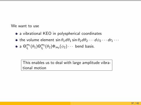
We want to use

a vibrational KEO in polyspherical coordinates

the volume element sin θ1dθ1 sin θ2dθ2 · · · dφ2 · · · dr1 · · ·a Θm1

l1(θ1)Θm2

l2(θ2)Φm2(φ2) · · · bend basis.

This enables us to deal with large amplitude vibra-tional motion

37 / 61

For any molecule-fixed axis system, the classical kinetic energy is,

Kclass =1

2

(J p

)(Grr Grv

G trv Gvv

)(Jp

)

38 / 61

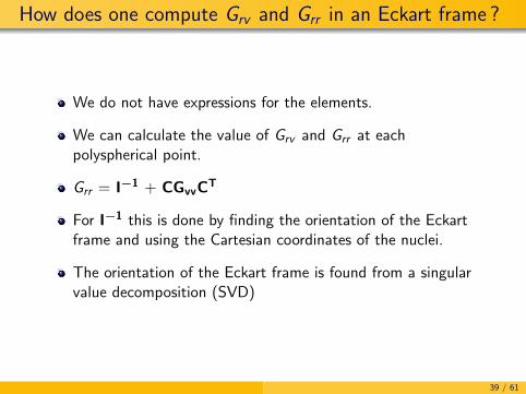
How does one compute Grv and Grr in an Eckart frame ?

We do not have expressions for the elements.

We can calculate the value of Grv and Grr at eachpolyspherical point.

Grr = I−1 + CGvvCT

For I−1 this is done by finding the orientation of the Eckartframe and using the Cartesian coordinates of the nuclei.

The orientation of the Eckart frame is found from a singularvalue decomposition (SVD)

39 / 61

For H2O numerical and analytic G matrix elements agreewell

At r1 = 1.7 bohr, r2 = 1.5 bohr, θ = 100◦

gv(1,1) 4× 10−14

gv(1,2) < 10−14

gv(1,3) < 10−14

gv(3,3) 2× 10−13

grv(2,1) < 10−14

grv(2,2) 1× 10−14

grv(2,3) < 10−14

grr(1,1) < 10−14

grr(3,3) 1× 10−14

grr(1,3) < 10−14

grr(2,2) < 10−14

40 / 61

Good convergence for J = 1 levels of methane

TABLE I: J = 1: convergence and comparison with previous calculations. Nb = 437

P = 2 P = 3 P = 4 P = 5

Nvib = 25 Nvib = 80 Nvib = 220 Nvib = 551 Theory Expt.

Ecutv =3100.

cm−1

Ecutv =4600.

cm−1

Ecutv =6200.

cm−1

Ecutv =7800.

cm−1

WC2004 Albert2009

.014 .001 .001 10.429 10.43 10.48 (F1)

.022 .022 .000 1312.410 1312.41 1311.43 (A2)

.014 .014 .000 1317.250 1317.25 1316.30 (F2)

.020 .018 .000 1326.727 1326.73 1325.82 (F1)

.019 .018 .000 1327.030 1327.03 1326.13 (E )

.015 .014 .000 1543.788 1543.79 1543.93 (F2)

.017 .017 .000 1543.910 1543.91 1544.05 (F1)

.122 .025 .023 2600.011 2600.02 2597.37 (F1) P=2 starts

· · · · · · · · · · · · · · · · · ·

.131 .020 .018 3075.813 3075.82 3076.01 (F1) P=2 ends

N.A. .293 .006 3875.859 3875.95 3871.56 (A2) P=3 starts

N.A. · · · · · · · · · · · · · · ·

N.A. .160 .002 4606.426 4606.50 4606.55 (F1) P=3 ends

1

41 / 61

Good convergence with Nvib, 200 is enough for J = 1

Good agreement with our previous calculations

75 basis functions are sufficient for the 75 states in P = 2

4 cm−1 errors (wrt expt) for Octad

42 / 61

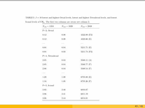
TABLE I: J = 10 lowest and highest Octad levels, lowest and highest Tetradecad levels, and lowest

Icosad levels of CH4. The first two columns are errors wrt column 3.

Nvib = 1210 Nvib = 1939 Nvib = 2949

P=3, Octad

0.12 0.08 4322.89 (F2)

0.12 0.08 4323.66 (E)

· · · · · · · · ·

0.04 0.04 5211.71 (E)

0.04 0.03 5211.74 (F2)

P=4, Tetradecad

2.05 0.04 5568.11 (A)

2.05 0.04 5568.77 (F)

2.06 0.04 5569.54 (F)

· · · · · ·

1.20 1.08 6755.08 (E)

1.16 1.05 6755.26 (F)

P=5, Icosad

2.92 2.40 6810.87

2.96 2.41 6811.19

3.06 2.44 6814.01

1

43 / 61

Convergence of J = 10 tetradecad levels

Red Nvib = 1210

Black Nvib = 1939

Benchmark Nvib = 2949

44 / 61

Determine a methane PES

Levels computed on pure ab initio surfaces are not accurateenough

For spectroscopic purposes the best pure ab initio surfaces arethose of Schwenke

Schwenke and Partridge (SP), Spectrochim. Acta A, 57,887(2001) CCSD(T) + cc-pVTZ

Schwenke, Spectrochim. Acta A, 58, 849 (2002) FCIextrapolation, CBS, all-electron, relativistic, Lamb shift,BODC, non-adiabatic

45 / 61

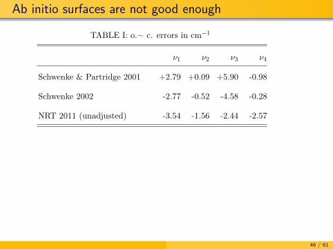
Ab initio surfaces are not good enough

TABLE I: o.− c. errors in cm−1

ν1 ν2 ν3 ν4

Schwenke & Partridge 2001 +2.79 +0.09 +5.90 -0.98

Schwenke 2002 -2.77 -0.52 -4.58 -0.28

NRT 2011 (unadjusted) -3.54 -1.56 -2.44 -2.57

1

46 / 61

Fit with the contracted Lanczos method

An efficient variational method makes it possible to refine aPES

We adjust 5 parameters of the SP PES, using only vibrationallevels.

47 / 61

Do not adjust the reference potential

To calculate vibrational levels we use a basis of products ofstretch and bend functions.

The stretch potential is Vs(θrefθrefθref , rrr) and the bend potential isVb(θθθ, r refr refr ref ).

48 / 61

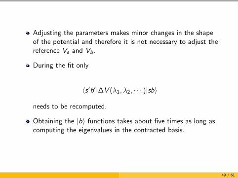
Adjusting the parameters makes minor changes in the shapeof the potential and therefore it is not necessary to adjust thereference Vs and Vb.

During the fit only

〈s ′b′|∆V (λ1, λ2, · · · )|sb〉

needs to be recomputed.

Obtaining the |b〉 functions takes about five times as long ascomputing the eigenvalues in the contracted basis.

49 / 61

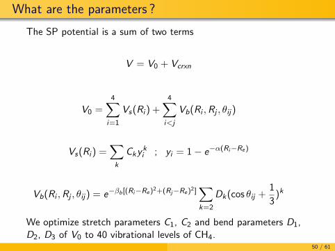
What are the parameters ?

The SP potential is a sum of two terms

V = V0 + Vcrxn

V0 =4∑

i=1

Vs(Ri ) +4∑

i<j

Vb(Ri ,Rj , θij )

Vs(Ri ) =∑

k

Ckyki ; yi = 1− e−α(Ri−Re)

Vb(Ri ,Rj , θij ) = e−βb[(Ri−Re)2+(Rj−Re)2]∑k=2

Dk(cos θij +1

3)k

We optimize stretch parameters C1, C2 and bend parameters D1,D2, D3 of V0 to 40 vibrational levels of CH4.

50 / 61

How good is the new surface ?

TABLE I: A comparison of the Schwenke-Partridge surface and the fitted surface.

SP PES fitted PES

RMSD (cm−1) 4.80 0.28

|∆Emax| (cm−1) 13.53 0.85

Re (A) 1.08900 1.08609

1

Re on the new surface agrees well with the best ab initio value(1.0859± 0.0003 (J. Stanton, Mol. Phys. 97, 841 (1999))).

51 / 61

How good is the PES for other isotopologues ?

O. N. Ulenikov, E. S. Bekhtereva, S Albert, H.-M. Niederer, S.Bauerecker, and M. Quack have studied many bands ofCH3D, CHD3, and CH2D2.

52 / 61

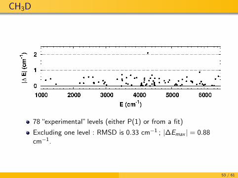
CH3D

78 “experimental” levels (either P(1) or from a fit)

Excluding one level : RMSD is 0.33 cm−1 ; |∆Emax | = 0.88cm−1.

53 / 61

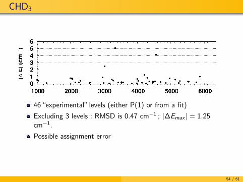
CHD3

46 “experimental” levels (either P(1) or from a fit)

Excluding 3 levels : RMSD is 0.47 cm−1 ; |∆Emax | = 1.25cm−1.

Possible assignment error

54 / 61

CH2D2

93 “experimental” levels (either P(1) or from a fit)

RMSD is 0.47 cm−1 ; |∆Emax | = 1.25 cm−1.

55 / 61

13CH4

37 “experimental” levels (either P(1) or from a fit)

RMSD is 0.27 cm−1 ; |∆Emax | = 0.77 cm−1.

56 / 61

Conclusion

Two problems impede the calculation of a ro-vibrationalspectrum using a KEO in polyspherical coordinates and acontracted basis.

In the standard basis vibrational eigenfunctions must becomputed for each K . For molecules for which vectors can bedefined so that θ1 = 0, π is inaccessible, this problem is solvedby taking m1 = −m2 −m3 − · · ·

With the standard choice of molecule-fixed axes thero-vibrational coupling is large. This problem can be solved byusing Eckart axes and computing G matrix elementsnumerically.

57 / 61

We can (finally) compute numerically exact ro-vibrationallevels of methane for high J.

A new PES is obtained by adjusting 5 parameters of SP PES

The errors on the new PES for the vibrational levels of 5methane isotopologues are consistently below 1 cm-1.

The same techniques can be applied to any molecule with 5atoms.

58 / 61

This work has been supported by

The Canadian Space Agency

The Reseau quebecois de calcul de haute performance,

The Canada Research Chairs programme

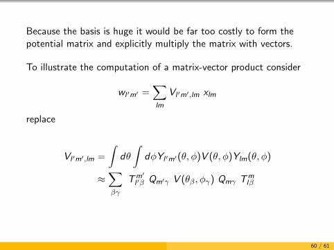
Because the basis is huge it would be far too costly to form thepotential matrix and explicitly multiply the matrix with vectors.

To illustrate the computation of a matrix-vector product consider

wl ′m′ =∑lm

Vl ′m′,lm xlm

replace

Vl ′m′,lm =

∫dθ

∫dφYl ′m′(θ, φ)V (θ, φ)Ylm(θ, φ)

≈∑βγ

Tm′l ′β Qm′γ V (θβ, φγ) Qmγ Tm

lβ

60 / 61

wl ′m′ =∑lm

∑βγ

Tm′l ′β Qm′γ V (θβ, φγ) Qmγ Tm

lβ xlm

wl ′m′ =∑β

Tm′l ′β

∑γ

Qm′γ V (θβ, φγ)∑

m

Qmγ

∑l

Tmlβ xlm

The largest vector is labelled by the grid indices.

61 / 61