246
Matthias Beck & Sinai Robins Computing the Continuous Discretely Integer-Point Enumeration in Polyhedra July 7, 2009 Springer Berlin Heidelberg NewYork Hong Kong London Milan Paris Tokyo
Matthias Beck & Sinai Robins
Computing the ContinuousDiscretely
Integer-Point Enumeration in Polyhedra
July 7, 2009
Springer
Berlin Heidelberg NewYorkHongKong LondonMilan Paris Tokyo


To Tendai To my mom, Michal Robins
with all our love.

Preface
The world is continuous, but the mind is discrete.
David Mumford
We seek to bridge some critical gaps between various fields of mathematics bystudying the interplay between the continuous volume and the discrete vol-ume of polytopes. Examples of polytopes in three dimensions include crystals,boxes, tetrahedra, and any convex object whose faces are all flat. It is amusingto see how many problems in combinatorics, number theory, and many othermathematical areas can be recast in the language of polytopes that exist insome Euclidean space. Conversely, the versatile structure of polytopes givesus number-theoretic and combinatorial information that flows naturally fromtheir geometry.
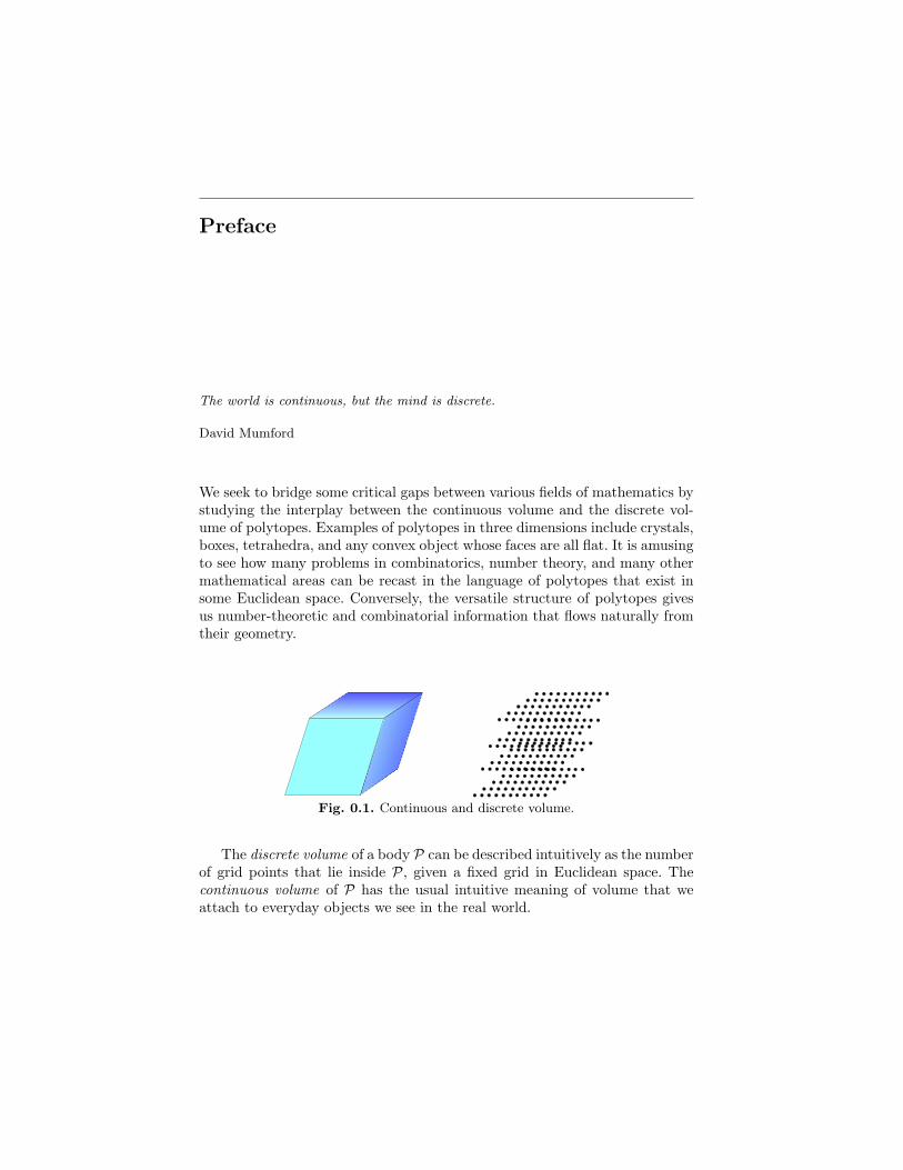
Fig. 0.1. Continuous and discrete volume.
The discrete volume of a body P can be described intuitively as the numberof grid points that lie inside P, given a fixed grid in Euclidean space. Thecontinuous volume of P has the usual intuitive meaning of volume that weattach to everyday objects we see in the real world.

VIII Preface
Indeed, the difference between the two realizations of volume can bethought of in physical terms as follows. On the one hand, the quantum-level grid imposed by the molecular structure of reality gives us a discretenotion of space and hence discrete volume. On the other hand, the New-tonian notion of continuous space gives us the continuous volume. We seethings continuously at the Newtonian level, but in practice we often computethings discretely at the quantum level. Mathematically, the grid we imposein space—corresponding to the grid formed by the atoms that make up anobject—helps us compute the usual continuous volume in very surprising andcharming ways, as we shall discover.
In order to see the continuous/discrete interplay come to life among thethree fields of combinatorics, number theory, and geometry, we begin our fo-cus with the simple-to-state coin-exchange problem of Frobenius. The beautyof this concrete problem is that it is easy to grasp, it provides a useful com-putational tool, and yet it has most of the ingredients of the deeper theoriesthat are developed here.
In the first chapter, we give detailed formulas that arise naturally fromthe Frobenius coin-exchange problem in order to demonstrate the intercon-nections between the three fields mentioned above. The coin-exchange problemprovides a scaffold for identifying the connections between these fields. In theensuing chapters we shed this scaffolding and focus on the interconnectionsthemselves:
(1) Enumeration of integer points in polyhedra—combinatorics,(2) Dedekind sums and finite Fourier series—number theory,(3) Polygons and polytopes—geometry.
We place a strong emphasis on computational techniques, and on com-puting volumes by counting integer points using various old and new ideas.Thus, the formulas we get should not only be pretty (which they are!) butshould also allow us to efficiently compute volumes by using some nice func-tions. In the very rare instances of mathematical exposition when we have aformulation that is both “easy to write” and “quickly computable,” we havefound a mathematical nugget. We have endeavored to fill this book with suchmathematical nuggets.
Much of the material in this book is developed by the reader in the morethan 200 exercises. Most chapters contain warm-up exercises that do not de-pend on the material in the chapter and can be assigned before the chapteris read. Some exercises are central, in the sense that current or later materialdepends on them. Those exercises are marked with ♣, and we give detailedhints for them at the end of the book. Most chapters also contain lists of openresearch problems.
It turns out that even a fifth grader can write an interesting paper oninteger-point enumeration [145], while the subject lends itself to deep inves-tigations that attract the current efforts of leading researchers. Thus, it is anarea of mathematics that attracts our innocent childhood questions as well
Preface IX
as our refined insight and deeper curiosity. The level of study is highly ap-propriate for a junior/senior undergraduate course in mathematics. In fact,this book is ideally suited to be used for a capstone course. Because the threetopics outlined above lend themselves to more sophisticated exploration, ourbook has also been used effectively for an introductory graduate course.
To help the reader fully appreciate the scope of the connections betweenthe continuous volume and the discrete volume, we begin the discourse in twodimensions, where we can easily draw pictures and quickly experiment. Wegently introduce the functions we need in higher dimensions (Dedekind sums)by looking at the coin-exchange problem geometrically as the discrete volumeof a generalized triangle, called a simplex.
The initial techniques are quite simple, essentially nothing more than ex-panding rational functions into partial fractions. Thus, the book is easily ac-cessible to a student who has completed a standard college calculus and linearalgebra curriculum. It would be useful to have a basic understanding of par-tial fraction expansions, infinite series, open and closed sets in Rd, complexnumbers (in particular, roots of unity), and modular arithmetic.
An important computational tool that is harnessed throughout the text isthe generating function f(x) =
∑∞m=0 a(m)xm, where the a(m)’s form any
sequence of numbers that we are interested in analyzing. When the infinitesequence of numbers a(m),m = 0, 1, 2, . . . , is embedded into a single generat-ing function f(x), it is often true that for hitherto unforeseen reasons, we canrewrite the whole sum f(x) in a surprisingly compact form. It is the rewritingof these generating functions that allows us to understand the combinatoricsof the relevant sequence a(m). For us, the sequence of numbers might be thenumber of ways to partition an integer into given coin denominations, or thenumber of points in an increasingly large body, and so on. Here we find yetanother example of the interplay between the discrete and the continuous: weare given a discrete set of numbers a(m), and we then carry out analysis onthe generating function f(x) in the continuous variable x.
What Is the Discrete Volume?
The physically intuitive description of the discrete volume given above restson a sound mathematical footing as soon as we introduce the notion of alattice. The grid is captured mathematically as the collection of all integerpoints in Euclidean space, namely Zd = {(x1, . . . , xd) : all xk ∈ Z}. Thisdiscrete collection of equally spaced points is called a lattice. If we are givena geometric body P, its discrete volume is simply defined as the number oflattice points inside P, that is, the number of elements in the set Zd ∩ P.
Intuitively, if we shrink the lattice by a factor k and count the numberof newly shrunken lattice points inside P, we obtain a better approximationfor the volume of P, relative to the volume of a single cell of the shrunkenlattice. It turns out that after the lattice is shrunk by an integer factor k, thenumber #
(P ∩ 1
kZd)
of shrunken lattice points inside an integral polytope P
X Preface
is magically a polynomial in k. This counting function #(P ∩ 1
kZd)
is knownas the Ehrhart polynomial of P. If we kept shrinking the lattice by taking alimit, we would of course end up with the continuous volume that is given bythe usual Riemannian integral definition of calculus:
volP = limk→∞
#(P ∩ 1
kZd)
1kd
.
However, pausing at fixed dilations of the lattice gives surprising flexibilityfor the computation of the volume of P and for the number of lattice pointsthat are contained in P.
Thus, when the body P is an integral polytope, the error terms that mea-sure the discrepancy between the discrete volume and the usual continuousvolume are quite nice; they are given by Ehrhart polynomials, and these enu-meration polynomials are the content of Chapter 3.
The Fourier–Dedekind Sums Are the Building Blocks: NumberTheory
Every polytope has a discrete volume that is expressible in terms of certainfinite sums that are known as Dedekind sums. Before giving their definition, wefirst motivate these sums with some examples that illustrate their building-block behavior for lattice-point enumeration. To be concrete, consider forexample a 1-dimensional polytope given by an interval P = [0, a], where a isany positive real number. It is clear that we need the greatest integer functionbxc to help us enumerate the lattice points in P, and indeed the answer isbac+ 1.
Next, consider a 1-dimensional line segment that is sitting in the 2-dimensional plane. Let’s pick our segment P so that it begins at the originand ends at the lattice point (c, d). As becomes apparent after a moment’sthought, the number of lattice points on this finite line segment involves anold friend, namely the greatest common divisor of c and d. The exact numberof lattice points on the line segment is gcd(c, d) + 1.
To unify both of these examples, consider a triangle P in the plane whosevertices have rational coordinates. It turns out that a certain finite sum iscompletely natural because it simultaneously extends both the greatest integerfunction and the greatest common divisor, although the latter is less obvious.An example of a Dedekind sum in two dimensions that arises naturally in theformula for the discrete volume of the rational triangle P is the following:
s(a, b) =b−1∑m=1
(m
b− 1
2
)(ma
b−⌊mab
⌋− 1
2
).
The definition makes use of the greatest integer function. Why do these sumsalso resemble the greatest common divisor? Luckily, the Dedekind sums sat-isfy a remarkable reciprocity law, quite similar to the Euclidean algorithm

Preface XI
that computes the gcd. This reciprocity law allows the Dedekind sums to becomputed in roughly log(b) steps rather than the b steps that are implied bythe definition above. The reciprocity law for s(a, b) lies at the heart of someamazing number theory that we treat in an elementary fashion, but that alsocomes from the deeper subject of modular forms and other modern tools.
We find ourselves in the fortunate position of viewing an important tip ofan enormous mountain of ideas, submerged by the waters of geometry. As wedelve more deeply into these waters, more and more hidden beauty unfoldsfor us, and the Dedekind sums are an indispensable tool that allow us to seefurther as the waters get deeper.
The Relevant Solids Are Polytopes: Geometry
The examples we have used, namely line segments and polygons in the plane,are special cases of polytopes in all dimensions. One way to define a polytopeis to consider the convex hull of a finite collection of points in Euclideanspace Rd. That is, suppose someone gives us a set of points v1, . . . ,vn inRd. The polytope determined by the given points vj is defined by all linearcombinations c1v1+c2v2+· · ·+cnvn, where the coefficients cj are nonnegativereal numbers that satisfy the relation c1 + c2 + · · ·+ cn = 1. This constructionis called the vertex description of the polytope.
There is another equivalent definition, called the hyperplane descriptionof the polytope. Namely, if someone hands us the linear inequalities thatdefine a finite collection of half-spaces in Rd, we can define the associatedpolytope as the simultaneous intersection of the half-spaces defined by thegiven inequalities.
There are some “obvious” facts about polytopes that are intuitively clearto most students but are, in fact, subtle and often nontrivial to prove from firstprinciples. Two of these facts, namely that every polytope has both a vertexand a hyperplane description, and that every polytope can be triangulated,form a crucial basis to the material we will develop in this book. We carefullyprove both facts in the appendices. The two main statements in the appen-dices are intuitively clear, so that novices can skip over their proofs withoutany detriment to their ability to compute continuous and discrete volumes ofpolytopes. All theorems in the text (including those in the appendices) areproved from first principles, with the exception of the last chapter, where weassume basic notions from complex analysis.
The text naturally flows into two parts, which we now explicate.
Part I
We have taken great care in making the content of the chapters flow seamlesslyfrom one to the next, over the span of the first six chapters.
• Chapters 1 and 2 introduce some basic notions of generating functions, inthe visually compelling context of discrete geometry, with an abundanceof detailed motivating examples.
XII Preface
Chapter 1The Coin-ExchangeProblem of Frobenius
@@R
?
Chapter 2A Gallery of Discrete Volumes
��
Chapter 3Counting Lattice Points inPolytopes: The Ehrhart Theory
?Chapter 7Finite Fourier Analysis
����
Chapter 4Reciprocity
?
�����9XXXXz
Chapter 8Dedekind Sums
Chapter 6Magic Squares
Chapter 5Face Numbers and theDehn–Sommerville Relations
CCW
Chapter 12A Discrete Version ofGreen’s Theorem
Chapter 9The Decomposition of aPolytope into Its Cones
�� @@R
Chapter 10Euler–MacLaurinSummation in Rd
Chapter 11Solid Angles
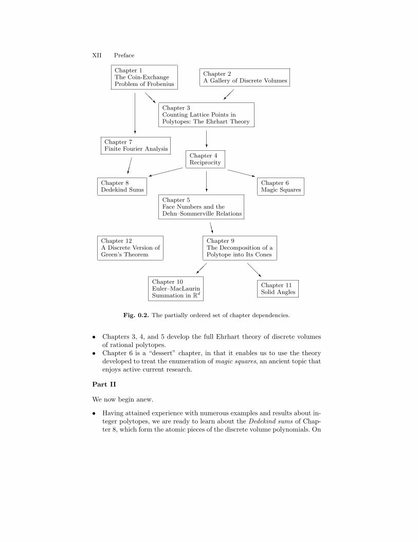
Fig. 0.2. The partially ordered set of chapter dependencies.
• Chapters 3, 4, and 5 develop the full Ehrhart theory of discrete volumesof rational polytopes.
• Chapter 6 is a “dessert” chapter, in that it enables us to use the theorydeveloped to treat the enumeration of magic squares, an ancient topic thatenjoys active current research.
Part II
We now begin anew.
• Having attained experience with numerous examples and results about in-teger polytopes, we are ready to learn about the Dedekind sums of Chap-ter 8, which form the atomic pieces of the discrete volume polynomials. On

Preface XIII
the other hand, to fully understand Dedekind sums, we need to understandfinite Fourier analysis, which we therefore develop from first principles inChapter 7, using only partial fractions.
• Chapter 9 answers a simple yet tricky question: how does the finite ge-ometric series in one dimension extend to higher-dimensional polytopes?Brion’s theorem give the elegant and decisive answer to this question.
• Chapter 10 extends the interplay between the continuous volume and thediscrete volume of a polytope (already studied in detail in Part I) byintroducing Euler–Maclaurin summation formulas in all dimensions. Theseformulas compare the continuous Fourier transform of a polytope to itsdiscrete Fourier transform, yet the material is completely self-contained.
• Chapter 11 develops an exciting extension of Ehrhart theory that definesand studies the solid angles of a polytope; these are the natural extensionsof 2-dimensional angles to higher dimensions.
• Finally, we end with another “dessert” chapter that uses complex ana-lytic methods to find an integral formula for the discrepancy between thediscrete and continuous areas enclosed by a closed curve in the plane.
Because polytopes are both theoretically useful (in triangulated manifolds,for example) and practically essential (in computer graphics, for example) weuse them to link results in number theory and combinatorics. There are manyresearch papers being written on these interconnections, even as we speak,and it is impossible to capture them all here; however, we hope that thesemodest beginnings will give the reader who is unfamiliar with these fields agood sense of their beauty, inexorable connectedness, and utility. We havewritten a gentle invitation to what we consider a gorgeous world of countingand of links between the fields of combinatorics, number theory, and geometryfor the general mathematical reader.
There are a number of excellent books that have a nontrivial intersec-tion with ours and contain material that complements the topics discussedhere. We heartily recommend the monographs of Barvinok [12] (on generalconvexity topics), Ehrhart [81] (the historic introduction to Ehrhart theory),Ewald [82] (on connections to algebraic geometry), Hibi [96] (on the interplayof algebraic combinatorics with polytopes), Miller–Sturmfels [132] (on com-putational commutative algebra), and Stanley [172] (on general enumerativeproblems in combinatorics).
Acknowledgments
We have had the good fortune of receiving help from many gracious peoplein the process of writing this book. First and foremost, we thank the stu-dents of the classes in which we could try out this material, at BinghamtonUniversity (SUNY), San Francisco State University, and Temple University.We are indebted to our MSRI/Banff 2005 graduate summer school students.We give special thanks to Kristin Camenga and Kevin Woods, who ran the
XIV Preface
problem sessions for this summer school, detected numerous typos, and pro-vided us with many interesting suggestions for this book. We are gratefulfor the generous support for the summer school from the Mathematical Sci-ences Research Institute, the Pacific Institute of Mathematics, and the BanffInternational Research Station.
Many colleagues supported this endeavor, and we are particularly grate-ful to everyone notifying us of mistakes, typos, and good suggestions: DanielAntonetti, Alexander Barvinok, Nathanael Berglund, Andrew Beyer, Tris-tram Bogart, Garry Bowlin, Benjamin Braun, Robin Chapman, Yitwah Che-ung, Jessica Cuomo, Dimitros Dais, Aaron Dall, Jesus De Loera, DavidDesario, Mike Develin, Ricardo Diaz, Michael Dobbins, Jeff Doker, HanMinh Duong, Richard Ehrenborg, Kord Eickmeyer, David Einstein, JosephGubeladze, Christian Haase, Mary Halloran, Friedrich Hirzebruch, BrianHopkins, Serkan Hosten, Benjamin Howard, Victor Katsnelson, Piotr Ma-ciak, Evgeny Materov, Asia Matthews, Peter McMullen, Martın Mereb, EzraMiller, Mel Nathanson, Yoshio Okamoto, Julian Pfeifle, Peter Pleasants, JorgeRamırez Alfonsın, Bruce Reznick, Adrian Riskin, Steven Sam, Junro Sato,Kim Seashore, Melissa Simmons, Richard Stanley, Bernd Sturmfels, ThorstenTheobald, Read Vanderbilt, Andrew Van Herick, Sven Verdoolaege, MicheleVergne, Julie Von Bergen, Neil Weickel, Carl Woll, Zhiqiang Xu, Jon Yag-gie, Ruriko Yoshida, Thomas Zaslavsky, Gunter Ziegler, and two anonymousreferees. We will collect corrections, updates, etc., at the Internet website
math.sfsu.edu/beck/ccd.html.
We are indebted to the Springer editorial staff, first and foremost to MarkSpencer, for facilitating the publication process in an always friendly andsupportive spirit. We thank David Kramer for the impeccable copyediting,Frank Ganz for sharing his LATEX expertise, and Felix Portnoy for the seamlessproduction process.
Matthias Beck would like to express his deepest gratitude to TendaiChitewere, for her patience, support, and unconditional love. He thanks hisfamily for always being there for him. Sinai Robins would like to thank MichalRobins, Shani Robins, and Gabriel Robins for their relentless support and un-derstanding during the completion of this project. We both thank all the cafeswe have inhabited over the past five years for enabling us to turn their coffeeinto theorems.
San Francisco Matthias BeckPhiladelphia Sinai RobinsJuly 2007
Contents
Part I The Essentials of Discrete Volume Computations
1 The Coin-Exchange Problem of Frobenius . . . . . . . . . . . . . . . . . 31.1 Why Use Generating Functions? . . . . . . . . . . . . . . . . . . . . . . . . . . . 31.2 Two Coins . . . . . . . . . . . . . . . . . . . . . . . . . . . . . . . . . . . . . . . . . . . . . . 51.3 Partial Fractions and a Surprising Formula . . . . . . . . . . . . . . . . . 71.4 Sylvester’s Result . . . . . . . . . . . . . . . . . . . . . . . . . . . . . . . . . . . . . . . . 111.5 Three and More Coins . . . . . . . . . . . . . . . . . . . . . . . . . . . . . . . . . . . 13Notes . . . . . . . . . . . . . . . . . . . . . . . . . . . . . . . . . . . . . . . . . . . . . . . . . . . . . . . 15Exercises . . . . . . . . . . . . . . . . . . . . . . . . . . . . . . . . . . . . . . . . . . . . . . . . . . . 17Open Problems . . . . . . . . . . . . . . . . . . . . . . . . . . . . . . . . . . . . . . . . . . . . . . 23
2 A Gallery of Discrete Volumes . . . . . . . . . . . . . . . . . . . . . . . . . . . . . 252.1 The Language of Polytopes . . . . . . . . . . . . . . . . . . . . . . . . . . . . . . . 252.2 The Unit Cube . . . . . . . . . . . . . . . . . . . . . . . . . . . . . . . . . . . . . . . . . . 262.3 The Standard Simplex . . . . . . . . . . . . . . . . . . . . . . . . . . . . . . . . . . . 292.4 The Bernoulli Polynomials as Lattice-Point Enumerators of
Pyramids . . . . . . . . . . . . . . . . . . . . . . . . . . . . . . . . . . . . . . . . . . . . . . . 312.5 The Lattice-Point Enumerators of the Cross-Polytopes . . . . . . . 352.6 Pick’s Theorem . . . . . . . . . . . . . . . . . . . . . . . . . . . . . . . . . . . . . . . . . 382.7 Polygons with Rational Vertices . . . . . . . . . . . . . . . . . . . . . . . . . . . 402.8 Euler’s Generating Function for General Rational Polytopes . . 45Notes . . . . . . . . . . . . . . . . . . . . . . . . . . . . . . . . . . . . . . . . . . . . . . . . . . . . . . . 48Exercises . . . . . . . . . . . . . . . . . . . . . . . . . . . . . . . . . . . . . . . . . . . . . . . . . . . 50Open Problems . . . . . . . . . . . . . . . . . . . . . . . . . . . . . . . . . . . . . . . . . . . . . . 54
3 Counting Lattice Points in Polytopes: The Ehrhart Theory 553.1 Triangulations and Pointed Cones . . . . . . . . . . . . . . . . . . . . . . . . . 553.2 Integer-Point Transforms for Rational Cones . . . . . . . . . . . . . . . . 583.3 Expanding and Counting Using Ehrhart’s Original Approach. . 623.4 The Ehrhart Series of an Integral Polytope . . . . . . . . . . . . . . . . . 65

XVI Contents
3.5 From the Discrete to the Continuous Volume of a Polytope . . . 693.6 Interpolation . . . . . . . . . . . . . . . . . . . . . . . . . . . . . . . . . . . . . . . . . . . . 713.7 Rational Polytopes and Ehrhart Quasipolynomials . . . . . . . . . . . 733.8 Reflections on the Coin-Exchange Problem and the Gallery
of Chapter 2 . . . . . . . . . . . . . . . . . . . . . . . . . . . . . . . . . . . . . . . . . . . . 74Notes . . . . . . . . . . . . . . . . . . . . . . . . . . . . . . . . . . . . . . . . . . . . . . . . . . . . . . . 74Exercises . . . . . . . . . . . . . . . . . . . . . . . . . . . . . . . . . . . . . . . . . . . . . . . . . . . 75Open Problems . . . . . . . . . . . . . . . . . . . . . . . . . . . . . . . . . . . . . . . . . . . . . . 80
4 Reciprocity . . . . . . . . . . . . . . . . . . . . . . . . . . . . . . . . . . . . . . . . . . . . . . . . 814.1 Generating Functions for Somewhat Irrational Cones . . . . . . . . . 824.2 Stanley’s Reciprocity Theorem for Rational Cones . . . . . . . . . . . 844.3 Ehrhart–Macdonald Reciprocity for Rational Polytopes . . . . . . 854.4 The Ehrhart Series of Reflexive Polytopes . . . . . . . . . . . . . . . . . . 864.5 More “Reflections” on Chapters 1 and 2 . . . . . . . . . . . . . . . . . . . . 88Notes . . . . . . . . . . . . . . . . . . . . . . . . . . . . . . . . . . . . . . . . . . . . . . . . . . . . . . . 88Exercises . . . . . . . . . . . . . . . . . . . . . . . . . . . . . . . . . . . . . . . . . . . . . . . . . . . 89Open Problems . . . . . . . . . . . . . . . . . . . . . . . . . . . . . . . . . . . . . . . . . . . . . . 91
5 Face Numbers and the Dehn–Sommerville Relations inEhrhartian Terms . . . . . . . . . . . . . . . . . . . . . . . . . . . . . . . . . . . . . . . . . 935.1 Face It! . . . . . . . . . . . . . . . . . . . . . . . . . . . . . . . . . . . . . . . . . . . . . . . . 935.2 Dehn–Sommerville Extended . . . . . . . . . . . . . . . . . . . . . . . . . . . . . . 955.3 Applications to the Coefficients of an Ehrhart Polynomial . . . . 965.4 Relative Volume . . . . . . . . . . . . . . . . . . . . . . . . . . . . . . . . . . . . . . . . . 98Notes . . . . . . . . . . . . . . . . . . . . . . . . . . . . . . . . . . . . . . . . . . . . . . . . . . . . . . . 100Exercises . . . . . . . . . . . . . . . . . . . . . . . . . . . . . . . . . . . . . . . . . . . . . . . . . . . 101
6 Magic Squares . . . . . . . . . . . . . . . . . . . . . . . . . . . . . . . . . . . . . . . . . . . . . 1036.1 It’s a Kind of Magic . . . . . . . . . . . . . . . . . . . . . . . . . . . . . . . . . . . . . 1046.2 Semimagic Squares: Points in the Birkhoff–von Neumann
Polytope . . . . . . . . . . . . . . . . . . . . . . . . . . . . . . . . . . . . . . . . . . . . . . . 1066.3 Magic Generating Functions and Constant-Term Identities . . . . 1096.4 The Enumeration of Magic Squares . . . . . . . . . . . . . . . . . . . . . . . . 114Notes . . . . . . . . . . . . . . . . . . . . . . . . . . . . . . . . . . . . . . . . . . . . . . . . . . . . . . . 115Exercises . . . . . . . . . . . . . . . . . . . . . . . . . . . . . . . . . . . . . . . . . . . . . . . . . . . 117Open Problems . . . . . . . . . . . . . . . . . . . . . . . . . . . . . . . . . . . . . . . . . . . . . . 118

Contents XVII
Part II Beyond the Basics
7 Finite Fourier Analysis . . . . . . . . . . . . . . . . . . . . . . . . . . . . . . . . . . . . 1217.1 A Motivating Example . . . . . . . . . . . . . . . . . . . . . . . . . . . . . . . . . . . 1217.2 Finite Fourier Series for Periodic Functions on Z . . . . . . . . . . . . 1237.3 The Finite Fourier Transform and Its Properties . . . . . . . . . . . . . 1277.4 The Parseval Identity . . . . . . . . . . . . . . . . . . . . . . . . . . . . . . . . . . . . 1297.5 The Convolution of Finite Fourier Series . . . . . . . . . . . . . . . . . . . . 131Notes . . . . . . . . . . . . . . . . . . . . . . . . . . . . . . . . . . . . . . . . . . . . . . . . . . . . . . . 132Exercises . . . . . . . . . . . . . . . . . . . . . . . . . . . . . . . . . . . . . . . . . . . . . . . . . . . 133
8 Dedekind Sums . . . . . . . . . . . . . . . . . . . . . . . . . . . . . . . . . . . . . . . . . . . . 1378.1 Fourier–Dedekind Sums and the Coin-Exchange Problem
Revisited . . . . . . . . . . . . . . . . . . . . . . . . . . . . . . . . . . . . . . . . . . . . . . . 1378.2 The Dedekind Sum and Its Reciprocity and Computational
Complexity . . . . . . . . . . . . . . . . . . . . . . . . . . . . . . . . . . . . . . . . . . . . . 1418.3 Rademacher Reciprocity for the Fourier–Dedekind Sum . . . . . . 1428.4 The Mordell–Pommersheim Tetrahedron . . . . . . . . . . . . . . . . . . . 145Notes . . . . . . . . . . . . . . . . . . . . . . . . . . . . . . . . . . . . . . . . . . . . . . . . . . . . . . . 148Exercises . . . . . . . . . . . . . . . . . . . . . . . . . . . . . . . . . . . . . . . . . . . . . . . . . . . 149Open Problems . . . . . . . . . . . . . . . . . . . . . . . . . . . . . . . . . . . . . . . . . . . . . . 151
9 The Decomposition of a Polytope into Its Cones . . . . . . . . . . . 1539.1 The Identity “
∑m∈Z z
m = 0” . . . or “Much Ado AboutNothing” . . . . . . . . . . . . . . . . . . . . . . . . . . . . . . . . . . . . . . . . . . . . . . . 153
9.2 Tangent Cones and Their Rational Generating Functions . . . . . 1579.3 Brion’s Theorem . . . . . . . . . . . . . . . . . . . . . . . . . . . . . . . . . . . . . . . . 1589.4 Brion Implies Ehrhart . . . . . . . . . . . . . . . . . . . . . . . . . . . . . . . . . . . . 160Notes . . . . . . . . . . . . . . . . . . . . . . . . . . . . . . . . . . . . . . . . . . . . . . . . . . . . . . . 161Exercises . . . . . . . . . . . . . . . . . . . . . . . . . . . . . . . . . . . . . . . . . . . . . . . . . . . 162
10 Euler–Maclaurin Summation in Rd . . . . . . . . . . . . . . . . . . . . . . . . . 16510.1 Todd Operators and Bernoulli Numbers . . . . . . . . . . . . . . . . . . . . 16510.2 A Continuous Version of Brion’s Theorem . . . . . . . . . . . . . . . . . . 16810.3 Polytopes Have Their Moments . . . . . . . . . . . . . . . . . . . . . . . . . . . 17010.4 From the Continuous to the Discrete Volume of a Polytope . . . 172Notes . . . . . . . . . . . . . . . . . . . . . . . . . . . . . . . . . . . . . . . . . . . . . . . . . . . . . . . 174Exercises . . . . . . . . . . . . . . . . . . . . . . . . . . . . . . . . . . . . . . . . . . . . . . . . . . . 175Open Problems . . . . . . . . . . . . . . . . . . . . . . . . . . . . . . . . . . . . . . . . . . . . . . 176
11 Solid Angles . . . . . . . . . . . . . . . . . . . . . . . . . . . . . . . . . . . . . . . . . . . . . . . 17711.1 A New Discrete Volume Using Solid Angles . . . . . . . . . . . . . . . . . 17711.2 Solid-Angle Generating Functions and a Brion-Type Theorem . 18011.3 Solid-Angle Reciprocity and the Brianchon–Gram Relations . . . 182

XVIII Contents
11.4 The Generating Function of Macdonald’s Solid-AnglePolynomials . . . . . . . . . . . . . . . . . . . . . . . . . . . . . . . . . . . . . . . . . . . . 186
Notes . . . . . . . . . . . . . . . . . . . . . . . . . . . . . . . . . . . . . . . . . . . . . . . . . . . . . . . 187Exercises . . . . . . . . . . . . . . . . . . . . . . . . . . . . . . . . . . . . . . . . . . . . . . . . . . . 187Open Problems . . . . . . . . . . . . . . . . . . . . . . . . . . . . . . . . . . . . . . . . . . . . . . 188
12 A Discrete Version of Green’s Theorem Using EllipticFunctions . . . . . . . . . . . . . . . . . . . . . . . . . . . . . . . . . . . . . . . . . . . . . . . . . . 18912.1 The Residue Theorem . . . . . . . . . . . . . . . . . . . . . . . . . . . . . . . . . . . . 18912.2 The Weierstraß ℘ and ζ Functions . . . . . . . . . . . . . . . . . . . . . . . . . 19112.3 A Contour-Integral Extension of Pick’s Theorem . . . . . . . . . . . . 193Notes . . . . . . . . . . . . . . . . . . . . . . . . . . . . . . . . . . . . . . . . . . . . . . . . . . . . . . . 194Exercises . . . . . . . . . . . . . . . . . . . . . . . . . . . . . . . . . . . . . . . . . . . . . . . . . . . 194Open Problems . . . . . . . . . . . . . . . . . . . . . . . . . . . . . . . . . . . . . . . . . . . . . . 195
Vertex and Hyperplane Descriptions of Polytopes . . . . . . . . . . . . . 197A.1 Every h-cone is a v-cone . . . . . . . . . . . . . . . . . . . . . . . . . . . . . . . . . . 198A.2 Every v-cone is an h-cone . . . . . . . . . . . . . . . . . . . . . . . . . . . . . . . . . 200
Triangulations of Polytopes . . . . . . . . . . . . . . . . . . . . . . . . . . . . . . . . . . . . 203
Hints for ♣ Exercises . . . . . . . . . . . . . . . . . . . . . . . . . . . . . . . . . . . . . . . . . . 207
References . . . . . . . . . . . . . . . . . . . . . . . . . . . . . . . . . . . . . . . . . . . . . . . . . . . . . 215
List of Symbols . . . . . . . . . . . . . . . . . . . . . . . . . . . . . . . . . . . . . . . . . . . . . . . . 225
Index . . . . . . . . . . . . . . . . . . . . . . . . . . . . . . . . . . . . . . . . . . . . . . . . . . . . . . . . . . 227

Part I
The Essentials of Discrete VolumeComputations

1
The Coin-Exchange Problem of Frobenius
The full beauty of the subject of generating functions emerges only from tuning inon both channels: the discrete and the continuous.
Herbert Wilf [187]
Suppose we’re interested in an infinite sequence of numbers (ak)∞k=0 that arisesgeometrically or recursively. Is there a “good formula” for ak as a function ofk? Are there identities involving various ak’s? Embedding this sequence intothe generating function
F (z) =∑k≥0
ak zk
allows us to retrieve answers to the questions above in a surprisingly quickand elegant way. We can think of F (z) as lifting our sequence ak from itsdiscrete setting into the continuous world of functions.
1.1 Why Use Generating Functions?
To illustrate these concepts, we warm up with the classic example of theFibonacci sequence fk, named after Leonardo Pisano Fibonacci (1170–1250?)1 and defined by the recursion
f0 = 0, f1 = 1, and fk+2 = fk+1 + fk for k ≥ 0 .
This gives the sequence (fk)∞k=0 = (0, 1, 1, 2, 3, 5, 8, 13, 21, 34, . . . ) (see also[165, Sequence A000045]). Now let’s see what generating functions can do forus. Let1 For more information about Fibonacci, seehttp://www-groups.dcs.st-and.ac.uk/∼history/Mathematicians/Fibonacci.html.
4 1 The Coin-Exchange Problem of Frobenius
F (z) =∑k≥0
fk zk.
We embed both sides of the recursion identity into their generating functions:∑k≥0
fk+2 zk =
∑k≥0
(fk+1 + fk) zk =∑k≥0
fk+1 zk +
∑k≥0
fk zk. (1.1)
The left–hand side of (1.1) is∑k≥0
fk+2 zk =
1z2
∑k≥0
fk+2 zk+2 =
1z2
∑k≥2
fk zk =
1z2
(F (z)− z) ,
while the right–hand side of (1.1) is∑k≥0
fk+1 zk +
∑k≥0
fk zk =
1zF (z) + F (z) .
So (1.1) can be restated as
1z2
(F (z)− z) =1zF (z) + F (z) ,
orF (z) =
z
1− z − z2.
It’s fun to check (e.g., with a computer) that when we expand the function Finto a power series, we indeed obtain the Fibonacci numbers as coefficients:
z
1− z − z2= z + z2 + 2 z3 + 3 z4 + 5 z5 + 8 z6 + 13 z7 + 21 z8 + 34 z9 + · · · .
Now we use our favorite method of handling rational functions: the par-tial fraction expansion. In our case, the denominator factors as 1 − z − z2 =(
1− 1+√
52 z
)(1− 1−
√5
2 z)
, and the partial fraction expansion is (see Exer-cise 1.1)
F (z) =z
1− z − z2=
1/√
5
1− 1+√
52 z
− 1/√
5
1− 1−√
52 z
. (1.2)
The two terms suggest the use of the geometric series∑k≥0
xk =1
1− x(1.3)
(see Exercise 1.2) with x = 1+√
52 z and x = 1−
√5
2 z, respectively:
F (z) =z
1− z − z2=
1√5
∑k≥0
(1 +√
52
z
)k− 1√
5
∑k≥0
(1−√
52
z
)k
=∑k≥0
1√5
(1 +√
52
)k−
(1−√
52
)k zk.
1.2 Two Coins 5
Comparing the coefficients of zk in the definition of F (z) =∑k≥0 fk z
k andthe new expression above for F (z), we discover the closed form expression forthe Fibonacci sequence
fk =1√5
(1 +√
52
)k− 1√
5
(1−√
52
)k.
This method of decomposing a rational generating function into partialfractions is one of our key tools. Because we will use partial fractions timeand again throughout this book, we record the result on which this methodis based.
Theorem 1.1 (Partial fraction expansion). Given any rational function
F (z) :=p(z)∏m
k=1 (z − ak)ek,
where p is a polynomial of degree less than e1 + e2 + · · ·+ em and the ak’s aredistinct, there exists a decomposition
F (z) =m∑k=1
(ck,1z − ak
+ck,2
(z − ak)2 + · · ·+ ck,ek(z − ak)ek
),
where ck,j ∈ C are unique.
One possible proof of this theorem is based on the fact that the polynomialsform a Euclidean domain. For readers who are acquainted with this notion,we outline this proof in Exercise 1.35.
1.2 Two Coins
Let’s imagine that we introduce a new coin system. Instead of using pennies,nickels, dimes, and quarters, let’s say we agree on using 4-cent, 7-cent, 9-cent,and 34-cent coins. The reader might point out the following flaw of this newsystem: certain amounts cannot be changed (that is, created with the availablecoins), for example, 2 or 5 cents. On the other hand, this deficiency makes ournew coin system more interesting than the old one, because we can ask thequestion, “which amounts can be changed?” In fact, we will prove in Exercise1.20 that there are only finitely many integer amounts that cannot be changedusing our new coin system. A natural question, first tackled by FerdinandGeorg Frobenius (1849–1917),2 and James Joseph Sylvester (1814–1897)3 is,2 For more information about Frobenius, seehttp://www-groups.dcs.st-and.ac.uk/∼history/Mathematicians/Frobenius.html.
3 For more information about Sylvester, seehttp://www-groups.dcs.st-and.ac.uk/∼history/Mathematicians/Sylvester.html.
6 1 The Coin-Exchange Problem of Frobenius
“what is the largest amount that cannot be changed?” As mathematicians,we like to keep questions as general as possible, and so we ask, given coins ofdenominations a1, a2, . . . , ad, which are positive integers without any commonfactor, can you give a formula for the largest amount that cannot be changedusing the coins a1, a2, . . . , ad? This problem is known as the Frobenius coin-exchange problem.
To be precise, suppose we’re given a set of positive integers
A = {a1, a2, . . . , ad}
with gcd (a1, a2, . . . , ad) = 1 and we call an integer n representable if thereexist nonnegative integers m1,m2, . . . ,md such that
n = m1a1 + · · ·+mdad .
In the language of coins, this means that we can change the amount n us-ing the coins a1, a2, . . . , ad. The Frobenius problem (often called the linearDiophantine problem of Frobenius) asks us to find the largest integer that isnot representable. We call this largest integer the Frobenius number anddenote it by g(a1, . . . , ad). The following theorem gives us a pretty formulafor d = 2.
Theorem 1.2. If a1 and a2 are relatively prime positive integers, then
g (a1, a2) = a1a2 − a1 − a2 .
This simple-looking formula for g inspired a great deal of research intoformulas for g (a1, a2, . . . , ad) with only limited success; see the notes at theend of this chapter. For d = 2, Sylvester gave the following result.
Theorem 1.3 (Sylvester’s theorem). Let a1 and a2 be relatively primepositive integers. Exactly half of the integers between 1 and (a1 − 1) (a2 − 1)are representable.
Our goal in this chapter is to prove these two theorems (and a little more)using the machinery of partial fractions. We approach the Frobenius problemthrough the study of the restricted partition function
pA(n) := #{
(m1, . . . ,md) ∈ Zd : all mj ≥ 0, m1a1 + · · ·+mdad = n},
the number of partitions of n using only the elements of A as parts.4 Inview of this partition function, g(a1, . . . , ad) is the largest integer n for whichpA(n) = 0.
There is a beautiful geometric interpretation of the restricted partitionfunction. The geometric description begins with the set4 A partition of a positive integer n is a multiset (i.e., a set in which we allow
repetition) {n1, n2, . . . , nk} of positive integers such that n = n1 + n2 + · · ·+ nk.The numbers n1, n2, . . . , nk are called the parts of the partition.
1.3 Partial Fractions and a Surprising Formula 7
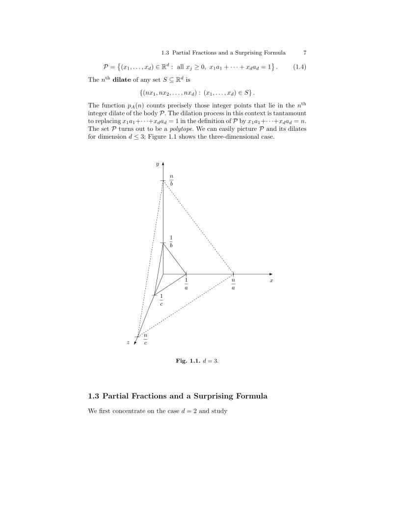
P ={
(x1, . . . , xd) ∈ Rd : all xj ≥ 0, x1a1 + · · ·+ xdad = 1}. (1.4)
The nth dilate of any set S ⊆ Rd is
{(nx1, nx2, . . . , nxd) : (x1, . . . , xd) ∈ S} .
The function pA(n) counts precisely those integer points that lie in the nth
integer dilate of the body P. The dilation process in this context is tantamountto replacing x1a1+· · ·+xdad = 1 in the definition of P by x1a1+· · ·+xdad = n.The set P turns out to be a polytope. We can easily picture P and its dilatesfor dimension d ≤ 3; Figure 1.1 shows the three-dimensional case.
x
y
z
1
a
1
b
1
c
n
a
n
b
n
c
Fig. 1.1. d = 3.
1.3 Partial Fractions and a Surprising Formula
We first concentrate on the case d = 2 and study
8 1 The Coin-Exchange Problem of Frobenius
p{a,b}(n) = #{
(k, l) ∈ Z2 : k, l ≥ 0, ak + bl = n}.
Recall that we require a and b to be relatively prime. To begin our discus-sion, we start playing with generating functions. Consider the product of thefollowing two geometric series:(
11− za
)(1
1− zb
)=(1 + za + z2a + · · ·
) (1 + zb + z2b + · · ·
)(see Exercise 1.2). If we multiply out all the terms we’ll get a power series allof whose exponents are linear combinations of a and b. In fact, the coefficientof zn in this power series counts the number of ways that n can be written asa nonnegative linear combination of a and b. In other words, these coefficientsare precisely evaluations of our counting function p{a,b}:(
11− za
)(1
1− zb
)=∑k≥0
∑l≥0
zakzbl =∑n≥0
p{a,b}(n) zn.
So this function is the generating function for the sequence of integers(p{a,b}(n)
)∞n=0
. The idea is now to study the compact function on the left.We would like to uncover an interesting formula for p{a,b}(n) by looking at
the generating function on the left more closely. To make our computationallife easier, we study the constant term of a related series; namely, p{a,b}(n) isthe constant term of
f(z) :=1
(1− za) (1− zb) zn=∑k≥0
p{a,b}(k) zk−n.
The latter series is not quite a power series, since it includes terms with neg-ative exponents. These series are called Laurent series, after Pierre AlphonseLaurent (1813–1854). For a power series (centered at 0), we could simply eval-uate the corresponding function at z = 0 to obtain the constant term; oncewe have negative exponents, such an evaluation is not possible. However, ifwe first subtract all terms with negative exponents, we’ll get a power serieswhose constant term (which remains unchanged) can now be computed byevaluating this remaining function at z = 0.
To be able to compute this constant term, we will expand f into partialfractions. As a warm-up to partial fraction decompositions, we first work outa one-dimensional example. Let’s denote the first ath root of unity by
ξa := e2πi/a = cos2πa
+ i sin2πa
;
then all the ath roots of unity are 1, ξa, ξ2a, ξ
3a, . . . , ξ
a−1a .
Example 1.4. Let’s find the partial fraction expansion of 11−za . The poles of
this function are located at all ath roots of unity ξka for k = 0, 1, . . . , a− 1. Sowe expand
1.3 Partial Fractions and a Surprising Formula 9
11− za
=a−1∑k=0
Ckz − ξka
.
How do we find the coefficients Ck? Well,
Ck = limz→ξka
(z − ξka
)( 11− za
)= limz→ξka
1−a za−1
= −ξka
a,
where we have used L’Hopital’s rule in the penultimate equality. Therefore,we arrive at the expansion
11− za
= −1a
a−1∑k=0
ξkaz − ξka
. ut
Returning to restricted partitions, the poles of f are located at z = 0 withmultiplicity n, at z = 1 with multiplicity 2, and at all the other ath and bth
roots of unity with multiplicity 1 because a and b are relatively prime. Henceour partial fraction expansion looks like
f(z) =A1
z+A2
z2+· · ·+An
zn+
B1
z − 1+
B2
(z − 1)2+a−1∑k=1
Ckz − ξka
+b−1∑j=1
Dj
z − ξjb. (1.5)
We invite the reader to compute the coefficients (Exercise 1.21)
Ck = − 1
a (1− ξkba ) ξk(n−1)a
, (1.6)
Dj = − 1
b(
1− ξjab)ξj(n−1)b
.
To compute B2, we multiply both sides of (1.5) by (z−1)2 and take the limitas z → 1 to obtain
B2 = limz→1
(z − 1)2
(1− za) (1− zb) zn=
1ab,
by applying L’Hopital’s rule twice, for example. For the more interesting con-stant B1, we compute
B1 = limz→1
(z − 1)
(1
(1− za) (1− zb) zn−
1ab
(z − 1)2
)=
1ab− 1
2a− 1
2b− n
ab,
again by applying L’Hopital’s rule.We don’t need to compute the coefficients A1, . . . , An, since they con-
tribute only to the terms with negative exponents, which we can safely ne-glect; these terms do not contribute to the constant term of f . Once we have
10 1 The Coin-Exchange Problem of Frobenius
the other coefficients, the constant term of the Laurent series of f is—as wesaid above—the following function evaluated at 0:
p{a,b}(n) =
B1
z − 1+
B2
(z − 1)2+a−1∑k=1
Ckz − ξka
+b−1∑j=1
Dj
z − ξjb
∣∣∣∣∣∣z=0
= −B1 +B2 −a−1∑k=1
Ckξka−b−1∑j=1
Dj
ξjb.
With (1.6) in hand, this simplifies to
p{a,b}(n) =12a
+12b
+n
ab+
1a
a−1∑k=1
1(1− ξkba )ξkna
+1b
b−1∑j=1
1(1− ξjab )ξjnb
. (1.7)
Encouraged by this initial success, we now proceed to analyze each sum in(1.7) with the hope of recognizing them as more familiar objects.
For the next step we need to define the greatest-integer function bxc,which denotes the greatest integer less than or equal to x. A close siblingto this function is the fractional-part function {x} = x − bxc. To readersnot familiar with the functions bxc and {x} we recommend working throughExercises 1.3–1.5.
What we’ll do next is studying a special case, namely b = 1. This isappealing because p{a,1}(n) simply counts integer points in an interval:
p{a,1}(n) = #{
(k, l) ∈ Z2 : k, l ≥ 0, ak + l = n}
= # {k ∈ Z : k ≥ 0, ak ≤ n}
= #{k ∈ Z : 0 ≤ k ≤ n
a
}=⌊na
⌋+ 1 .
(See Exercise 1.3.) On the other hand, in (1.7) we just computed a differentexpression for this function, so that
12a
+12
+n
a+
1a
a−1∑k=1
1(1− ξka) ξkna
= p{a,1}(n) =⌊na
⌋+ 1 .
With the help of the fractional-part function {x} = x− bxc, we have deriveda formula for the following sum over ath roots of unity:
1a
a−1∑k=1
1(1− ξka) ξkna
= −{na
}+
12− 1
2a. (1.8)
We’re almost there: we invite the reader (Exercise 1.22) to show that
1.4 Sylvester’s Result 11
1a
a−1∑k=1
1(1− ξbka ) ξkna
=1a
a−1∑k=1
1(1− ξka) ξb−1kn
a
, (1.9)
where b−1 is an integer such that b−1b ≡ 1 mod a, and to conclude that
1a
a−1∑k=1
1(1− ξbka ) ξkna
= −{b−1n
a
}+
12− 1
2a. (1.10)
Now all that’s left to do is to substitute this expression back into (1.7), whichyields the following beautiful formula due to Tiberiu Popoviciu (1906–1975).
Theorem 1.5 (Popoviciu’s theorem). If a and b are relatively prime, then
p{a,b}(n) =n
ab−{b−1n
a
}−{a−1n
b
}+ 1 ,
where b−1b ≡ 1 mod a and a−1a ≡ 1 mod b. ut
1.4 Sylvester’s Result
Before we apply Theorem 1.5 to obtain the classical Theorems 1.2 and 1.3, wereturn for a moment to the geometry behind the restricted partition functionp{a,b}(n). In the two-dimensional case (which is the setting of Theorem 1.5),we are counting integer points (x, y) ∈ Z2 on the line segments defined by theconstraints
ax+ by = n , x, y ≥ 0 .
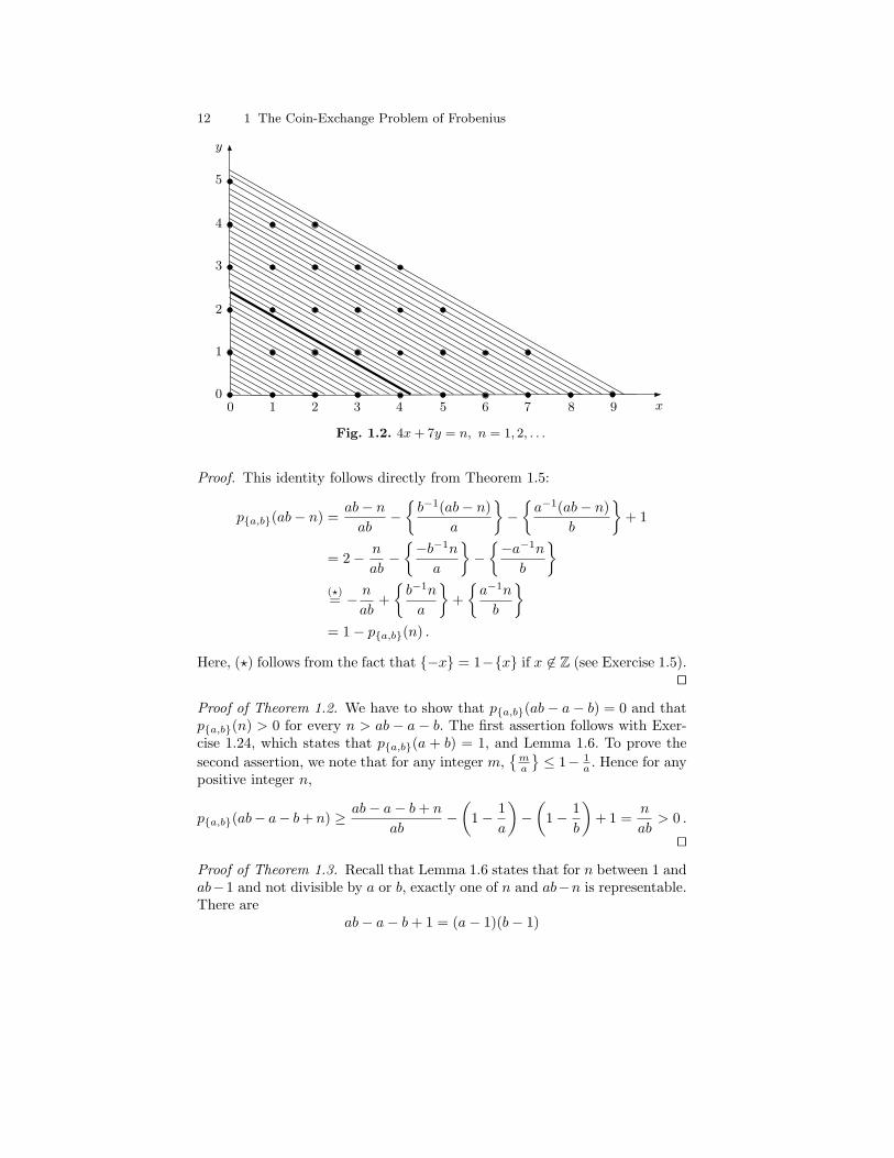
As n increases, the line segment gets dilated. It is not too far-fetched (al-though Exercise 1.13 teaches us to be careful with such statements) to expectthat the likelihood for an integer point to lie on the line segment increaseswith n. In fact, one might even guess that the number of points on the linesegment increases linearly with n, since the line segment is a one-dimensionalobject. Theorem 1.5 quantifies the previous statement in a very precise form:p{a,b}(n) has the “leading term” n/ab, and the remaining terms are boundedas functions in n. Figure 1.2 shows the geometry behind the counting func-tion p{4,7}(n) for the first few values of n. Note that the thick line segmentfor n = 17 = 4 · 7 − 4 − 7 is the last one that does not contain any integerpoint.
Lemma 1.6. If a and b are relatively prime positive integers and n ∈ [1, ab−1]is not a multiple of a or b, then
p{a,b}(n) + p{a,b}(ab− n) = 1 .
In other words, for n between 1 and ab− 1 and not divisible by a or b, exactlyone of the two integers n and ab− n is representable in terms of a and b.
12 1 The Coin-Exchange Problem of Frobenius
x0 1 2 3 4 5 6 7 8 9
y
0
1
2
3
4
5
Fig. 1.2. 4x+ 7y = n, n = 1, 2, . . .
Proof. This identity follows directly from Theorem 1.5:
p{a,b}(ab− n) =ab− nab
−{b−1(ab− n)
a
}−{a−1(ab− n)
b
}+ 1
= 2− n
ab−{−b−1n
a
}−{−a−1n
b
}(?)= − n
ab+{b−1n
a
}+{a−1n
b
}= 1− p{a,b}(n) .
Here, (?) follows from the fact that {−x} = 1−{x} if x 6∈ Z (see Exercise 1.5).ut
Proof of Theorem 1.2. We have to show that p{a,b}(ab− a− b) = 0 and thatp{a,b}(n) > 0 for every n > ab − a − b. The first assertion follows with Exer-cise 1.24, which states that p{a,b}(a + b) = 1, and Lemma 1.6. To prove thesecond assertion, we note that for any integer m,
{ma
}≤ 1− 1
a . Hence for anypositive integer n,
p{a,b}(ab− a− b+ n) ≥ ab− a− b+ n
ab−(
1− 1a
)−(
1− 1b
)+ 1 =
n
ab> 0 .
ut
Proof of Theorem 1.3. Recall that Lemma 1.6 states that for n between 1 andab−1 and not divisible by a or b, exactly one of n and ab−n is representable.There are
ab− a− b+ 1 = (a− 1)(b− 1)
1.5 Three and More Coins 13
integers between 1 and ab − 1 that are not divisible by a or b. Finally, wenote that p{a,b}(n) > 0 if n is a multiple of a or b, by the very definition ofp{a,b}(n). Hence the number of nonrepresentable integers is 1
2 (a−1)(b−1). ut
Note that we have proved even more. Essentially by Lemma 1.6, everypositive integer less than ab has at most one representation. Hence, the rep-resentable integers less than ab are uniquely representable (see also Exer-cise 1.25).
1.5 Three and More Coins
What happens to the complexity of the Frobenius problem if we have morethan two coins? Let’s go back to our restricted partition function
pA(n) = #{
(m1, . . . ,md) ∈ Zd : all mj ≥ 0, m1a1 + · · ·+mdad = n},
where A = {a1, . . . , ad}. By the very same reasoning as in Section 1.3, we caneasily write down the generating function for pA(n):∑
n≥0
pA(n) zn =(
11− za1
)(1
1− za2
)· · ·(
11− zad
).
We use the same methods that were exploited in Section 1.3 to recover ourfunction pA(n) as the constant term of a useful generating function. Namely,
pA(n) = const(
1(1− za1) (1− za2) · · · (1− zad) zn
).
We now expand the function on the right into partial fractions. For reasonsof simplicity we assume in the following that a1, . . . , ad are pairwise relativelyprime; that is, no two of the integers a1, a2, . . . , ad have a common factor.Then our partial fraction expansion looks like
f(z) =1
(1− za1) · · · (1− zad) zn
=A1
z+A2
z2+ · · ·+ An
zn+
B1
z − 1+
B2
(z − 1)2+ · · ·+ Bd
(z − 1)d(1.11)
+a1−1∑k=1
C1k
z − ξka1
+a2−1∑k=1
C2k
z − ξka2
+ · · ·+ad−1∑k=1
Cdkz − ξkad
.
By now we’re experienced in computing partial fraction coefficients, so thatthe reader will easily verify that (Exercise 1.29)
C1k = − 1
a1
(1− ξka2
a1
)(1− ξka3
a1
)· · ·(
1− ξkada1
)ξk(n−1)a1
. (1.12)

14 1 The Coin-Exchange Problem of Frobenius
As before, we don’t have to compute the coefficients A1, . . . , An, because theydon’t contribute to the constant term of f . For the computation of B1, . . . , Bd,we may use a symbolic manipulation program such as Maple or Mathematica.Again, once we have calculated these coefficients, we can compute the constantterm of f by dropping all negative exponents and evaluating the remainingfunction at 0:
pA(n) =
(B1
z − 1+ · · ·+ Bd
(z − 1)d+a1−1∑k=1
C1k
z − ξka1
+ · · ·+ad−1∑k=1
Cdkz − ξkad
)∣∣∣∣∣z=0
= −B1 +B2 − · · ·+ (−1)dBd −a1−1∑k=1
C1k
ξka1
−a2−1∑k=1
C2k
ξka2
− · · · −ad−1∑k=1
Cdkξkad
.
Substituting the expression we found for C1k into the latter sum over thenontrivial ath
1 roots of unity, for example, gives rise to
1a1
a1−1∑k=1
1(1− ξka2
a1
)(1− ξka3
a1
)· · ·(
1− ξkada1
)ξkna1
.
This motivates the definition of the Fourier–Dedekind sum
sn (a1, a2, . . . , am; b) :=1b
b−1∑k=1
ξknb(1− ξka1
b
)(1− ξka2
b
)· · ·(
1− ξkamb
) . (1.13)
We will study these sums in detail in Chapter 8. With this definition, we havearrived at the following result.
Theorem 1.7. The restricted partition function for A = {a1, a2, . . . , ad},where the ak’s are pairwise relatively prime, can be computed as
pA(n) = −B1 +B2 − · · ·+ (−1)dBd + s−n (a2, a3, . . . , ad; a1)+ s−n (a1, a3, a4, . . . , ad; a2) + · · ·+ s−n (a1, a2, . . . , ad−1; ad) .
Here B1, B2, . . . , Bd are the partial fraction coefficients in the expansion(1.11). ut
Example 1.8. We give the restricted partition functions for d = 3 and 4.These closed-form formulas have proven useful in the refined analysis of theperiodicity that is inherent in the restricted partition function pA(n). Forexample, one can visualize the graph of p{a,b,c}(n) as a “wavy parabola,” asits formula plainly shows.
Notes 15
p{a,b,c}(n) =n2
2abc+n
2
(1ab
+1ac
+1bc
)+
112
(3a
+3b
+3c
+a
bc+
b
ac+
c
ab
)+
1a
a−1∑k=1
1(1− ξkba ) (1− ξkca ) ξkna
+1b
b−1∑k=1
1(1− ξkcb
) (1− ξkab
)ξknb
+1c
c−1∑k=1
1(1− ξkac ) (1− ξkbc ) ξknc
,
p{a,b,c,d}(n) =n3
6abcd+n2
4
(1abc
+1abd
+1acd
+1bcd
)+
n
12
(3ab
+3ac
+3ad
+3bc
+3bd
+3cd
+a
bcd+
b
acd+
c
abd+
d
abc
)+
124
(a
bc+
a
bd+
a
cd+
b
ad+
b
ac+
b
cd+
c
ab+
c
ad+
c
bd
+d
ab+
d
ac+d
bc
)− 1
8
(1a
+1b
+1c
+1d
)+
1a
a−1∑k=1
1(1− ξkba ) (1− ξkca ) (1− ξkda ) ξkna
+1b
b−1∑k=1
1(1− ξkcb
) (1− ξkdb
) (1− ξkab
)ξknb
+1c
c−1∑k=1
1(1− ξkdc ) (1− ξkac ) (1− ξkbc ) ξknc
+1d
d−1∑k=1
1(1− ξkad
) (1− ξkbd
) (1− ξkcd
)ξknd
. ut
Notes
1. The theory of generating functions has a long and powerful tradition. Weonly touch on its utility. For those readers who would like to dig a littledeeper into the vast generating-function garden, we strongly recommend HerbWilf’s generatingfunctionology [187] and Laszlo Lovasz’s Combinatorial Prob-lems and Exercises [122]. The reader might wonder why we do not stressconvergence aspects of the generating functions we play with. Almost all ofour series are geometric series and have trivial convergence properties. In thespirit of not muddying the waters of lucid mathematical exposition, we omitsuch convergence details.
2. The Frobenius problem is named after Georg Frobenius, who apparentlyliked to raise this problem in his lectures [41]. Theorem 1.2 is one of the

16 1 The Coin-Exchange Problem of Frobenius
famous folklore results and might be one of the most misquoted theoremsin all of mathematics. People usually cite James J. Sylvester’s problem in[177], but his paper contains Theorem 1.3 rather than 1.2. In fact, Sylvester’sproblem had previously appeared as a theorem in [176]. It is not known whofirst discovered or proved Theorem 1.2. It is very conceivable that Sylvesterknew about it when he came up with Theorem 1.3.
3. The linear Diophantine problem of Frobenius should not be confused withthe postage-stamp problem. The latter problem asks for a similar determina-tion, but adds an additional independent bound on the size of the integersolutions to the linear equation.
4. Theorem 1.5 has an interesting history. The earliest appearance of thisresult that we are aware of is in a paper by Tiberiu Popoviciu [148]. Popoviciu’sformula has since been resurrected at least twice [161, 183].
5. Fourier–Dedekind sums first surfaced implicitly in Sylvester’s work (see,e.g., [175]) and explicitly in connection with restricted partition functionsin [104]. They were rediscovered in [25], in connection with the Frobeniusproblem. The papers [83, 157] contain interesting connections to Bernoulliand Euler polynomials. We will resume the study of the Fourier–Dedekindsums in Chapter 8.
6. As we already mentioned above, the Frobenius problem for d ≥ 3 is muchharder than the case d = 2 that we have discussed. Certainly beyond d = 3,the Frobenius problem is wide open, though much effort has been put into itsstudy. The literature on the Frobenius problem is vast, and there is still muchroom for improvement. The interested reader might consult the comprehensivemonograph [153], which surveys the references to almost all articles dealingwith the Frobenius problem and gives about 40 open problems and conjecturesrelated to the Frobenius problem. To give a flavor, we mention two landmarkresults that go beyond d = 2.
The first one concerns the generating function r(z) :=∑k∈R z
k, whereR is the set of all integers representable by a given set of relatively primepositive integers a1, a2, . . . , ad. It is not hard to see (Exercise 1.34) thatr(z) = p(z)/ (1− za1) (1− za2) · · · (1− zad) for some polynomial p. This ra-tional generating function contains all the information about the Frobeniusproblem; for example, the Frobenius number is the total degree of the function
11−z − r(z). Hence the Frobenius problem reduces to finding the polynomialp, the numerator of r. Marcel Morales [134, 135] and Graham Denham [73]discovered the remarkable fact that for d = 3, the polynomial p has either 4or 6 terms. Moreover, they gave semi-explicit formulas for p. The Morales–Denham theorem implies that the Frobenius number in the case d = 3 isquickly computable, a result that is originally due, in various disguises, toJurgen Herzog [95], Harold Greenberg [89], and J. Leslie Davison [65]. As
Exercises 17
much as there seems to be a well-defined border between the cases d = 2and d = 3, there also seems to be such a border between the cases d = 3and d = 4: Henrik Bresinsky [43] proved that for d ≥ 4, there is no absolutebound for the number of terms in the numerator p, in sharp contrast to theMorales–Denham theorem.
On the other hand, Alexander Barvinok and Kevin Woods [14] provedthat for fixed d, the rational generating function r(z) can be written as a“short” sum of rational functions; in particular, r can be efficiently computedwhen d is fixed. A corollary of this fact is that the Frobenius number canbe efficiently computed when d is fixed; this theorem is due to Ravi Kannan[105]. On the other hand, Jorge Ramırez-Alfonsın [152] proved that trying toefficiently compute the Frobenius number is hopeless if d is left as a variable.
While the above results settle the theoretical complexity of the computa-tion of the Frobenius number, practical algorithms are a completely differentmatter. Both Kannan’s and Barvinok–Woods’s ideas seem complex enoughthat nobody has yet tried to implement them. Currently, the fastest algo-rithm is presented in [32].
Exercises
1.1. ♣ Check the partial fraction expansion (1.2):
z
1− z − z2=
1/√
5
1− 1+√
52 z
− 1/√
5
1− 1−√
52 z
.
1.2. ♣ Suppose z is a complex number, and n is a positive integer. Show that
(1− z)(1 + z + z2 + · · ·+ zn
)= 1− zn+1,
and use this to prove that if |z| < 1,∑k≥0
zk =1
1− z.
1.3. ♣ Find a formula for the number of lattice points in [a, b] for arbitraryreal numbers a and b.
1.4. Prove the following. Unless stated differently, n ∈ Z and x, y ∈ R.
(a) bx+ nc = bxc+ n.(b) bxc+ byc ≤ bx+ yc ≤ bxc+ byc+ 1.
(c) bxc+ b−xc ={
0 if x ∈ Z,−1 otherwise.
(d) For n ∈ Z>0,⌊bxcn
⌋=⌊xn
⌋.
(e) −b−xc is the least integer greater than or equal to x, denoted by dxe.

18 1 The Coin-Exchange Problem of Frobenius
(f) bx+ 1/2c is the nearest integer to x (and if two integers are equally nearto x, it is the larger of the two).
(g) bxc+ bx+ 1/2c = b2xc.(h) If m and n are positive integers,
⌊mn
⌋is the number of integers among
1, . . . ,m that are divisible by n.(i) ♣ If m ∈ Z>0, n ∈ Z, then
⌊n−1m
⌋= −
⌊−nm
⌋− 1.
(j) ♣ If m ∈ Z>0, n ∈ Z, then⌊n−1m
⌋+ 1 is the least integer greater than or
equal to n/m.
1.5. Rewrite in terms of the fractional-part function as many of the aboveidentities as you can make sense of.
1.6. Suppose m and n are relatively prime positive integers. Prove that
m−1∑k=0
⌊kn
m
⌋=n−1∑j=0
⌊jm
n
⌋=
12
(m− 1)(n− 1) .
1.7. Prove the following identities. They will become handy at least twice:when we study partial fractions, and when we discuss finite Fourier series. Forφ, ψ ∈ R, n ∈ Z>0,m ∈ Z,
(a) ei0 = 1,(b) eiφ eiψ = ei(φ+ψ),(c) 1/eiφ = e−iφ,(d) ei(φ+2π) = eiφ,(e) e2πi = 1,(f)∣∣eiφ∣∣ = 1,
(g) ddφ e
iφ = i eiφ,
(h)∑n−1k=0 e
2πikm/n ={n if n|m,0 otherwise,
(i)∑n−1k=1 k e
2πik/n = ne2πi/n−1
.
1.8. Suppose m,n ∈ Z and n > 0. Find a closed form for∑n−1k=0
{kn
}e2πikm/n
(as a function of m and n).
1.9. ♣ Suppose m and n are relatively prime integers, and n is positive. Showthat {
e2πimk/n : 0 ≤ k < n}
={e2πij/n : 0 ≤ j < n
}and {
e2πimk/n : 0 < k < n}
={e2πij/n : 0 < j < n
}.
Conclude that if f is any complex-valued function, then
n−1∑k=0
f(e2πimk/n
)=n−1∑j=0
f(e2πij/n
)
Exercises 19
andn−1∑k=1
f(e2πimk/n
)=n−1∑j=1
f(e2πij/n
).
1.10. Suppose n is a positive integer. If you know what a group is, provethat the set
{e2πik/n : 0 ≤ k < n
}forms a cyclic group of order n (under
multiplication in C).
1.11. Fix n ∈ Z>0. For an integer m, let (m mod n) denote the least nonneg-ative integer in G1 := Zn to which m is congruent. Let’s denote by ? additionmodulo n, and by ◦ the following composition:{m1
n
}◦{m2
n
}={m1 +m2
n
},
defined on the set G2 :={{
mn
}: m ∈ Z
}. Define the following functions:
φ ((m mod n)) = e2πim/n,
ψ(e2πim/n
)={mn
},
χ({m
n
})= (m mod n) .
Prove the following:
φ ((m1 mod n) ? (m2 mod n)) = φ ((m1 mod n))φ ((m2 mod n)) ,
ψ(e2πim1/ne2πim2/n
)= ψ
(e2πim1/n
)◦ ψ(e2πim2/n
),
χ({m1
n
}◦{m2
n
})= χ
({m1
n
})? χ({m2
n
}).
Prove that the three maps defined above, namely φ, ψ, and χ, are one-to-one.Again, for the reader who is familiar with the notion of a group, let G3 bethe group of nth roots of unity. What we have shown is that the three groupsG1, G2, and G3 are all isomorphic. It is very useful to cycle among these threeisomorphic groups.
1.12. ♣ Given integers a, b, c, d, form the line segment in R2 joining the point(a, b) to (c, d). Show that the number of integer points on this line segment isgcd(a− c, b− d) + 1.
1.13. Give an example of a line with
(a) no lattice point;(b) one lattice point;(c) an infinite number of lattice points.
In each case, state—if appropriate—necessary conditions about the (ir)rationa-lity of the slope.
20 1 The Coin-Exchange Problem of Frobenius
1.14. Suppose a line y = mx+ b passes through the lattice points (p1, q1) and(p2, q2). Prove that it also passes through the lattice points(
p1 + k(p2 − p1), q1 + k(q2 − q1)), k ∈ Z .
1.15. Given positive irrational numbers p and q with 1p + 1
q = 1, show thatZ>0 is the disjoint union of the two integer sequences {bpnc : n ∈ Z>0} and{bqnc : n ∈ Z>0}. This theorem from 1894 is due to Lord Rayleigh and wasrediscovered in 1926 by Sam Beatty. Sequences of the form {bpnc : n ∈ Z>0}are often called Beatty sequences.
1.16. Let a, b, c, d ∈ Z. We say that {(a, b) , (c, d)} is a lattice basis of Z2 ifany lattice point (m,n) ∈ Z2 can be written as
(m,n) = p (a, b) + q (c, d)
for some p, q ∈ Z. Prove that if {(a, b) , (c, d)} and {(e, f) , (g, h)} are latticebases of Z2 then there exists an integer matrix M with determinant ±1 suchthat (
a bc d
)= M
(e fg h
).
Conclude that the determinant of(a bc d
)is ±1.
1.17. ♣ Prove that a triangle with vertices on the integer lattice has no otherinterior/boundary lattice points if and only if it has area 1
2 . (Hint: You maybegin by “doubling” the triangle to form a parallelogram.)
1.18. Let’s define a northeast lattice path as a path through lattice points thatuses only the steps (1, 0) and (0, 1). Let Ln be the line defined by x+ 2y = n.Prove that the number of northeast lattice paths from the origin to a latticepoint on Ln is the (n+ 1)th Fibonacci number fn+1.
1.19. Compute the coefficients of the Taylor series of 1/(1− z)2 expanded atz = 0
(a) by a counting argument,(b) by differentiating the geometric series.
Generalize.
1.20. ♣ Prove that if a1, a2, . . . , ad ∈ Z>0 do not have a common factor thenthe Frobenius number g(a1, . . . , ad) is well defined.
1.21. ♣ Compute the partial fraction coefficients (1.6).
Exercises 21
1.22. ♣ Prove (1.9): For relatively prime positive integers a and b,
1a
a−1∑k=1
1(1− ξbka ) ξkna
=1a
a−1∑k=1
1(1− ξka) ξb−1kn
a
,
where b−1b ≡ 1 mod a, and deduce from this (1.10), namely,
1a
a−1∑k=1
1(1− ξbka ) ξkna
= −{b−1n
a
}+
12− 1
2a.
(Hint: Use Exercise 1.9.)
1.23. Prove that for relatively prime positive integers a and b,
p{a,b}(n+ ab) = p{a,b}(n) + 1 .
1.24. ♣ Show that if a and b are relatively prime positive integers, then
p{a,b}(a+ b) = 1 .
1.25. To extend the Frobenius problem, let us call an integer n k-representableif pA(n) = k; that is, n can be represented in exactly k ways using the integersin the set A. Define gk = gk(a1, . . . , ad) to be the largest k-representableinteger. Prove:
(a) Let d = 2. For any k ∈ Z≥0 there is an N such that all integers larger thanN have at least k representations (and hence gk(a, b) is well defined).
(b) gk(a, b) = (k + 1)ab− a− b.(c) Given k ≥ 2, the smallest k-representable integer is ab(k − 1).(d) The smallest interval containing all uniquely representable integers is
[min(a, b), g1(a, b)].(e) Given k ≥ 2, the smallest interval containing all k-representable integers
is [gk−2(a, b) + a+ b, gk(a, b)].(f) There are exactly ab − 1 integers that are uniquely representable. Given
k ≥ 2, there are exactly ab k-representable integers.(g) Extend all of this to d ≥ 3 (see open problems).
1.26. Find a formula for p{a}(n).
1.27. Prove the following recursion formula:
p{a1,...,ad}(n) =∑m≥0
p{a1,...,ad−1}(n−mad) .
(Here we use the convention that pA(n) = 0 if n < 0.) Use it in the case d = 2to give an alternative proof of Theorem 1.2.

22 1 The Coin-Exchange Problem of Frobenius
1.28. Prove the following extension of Theorem 1.5: Suppose gcd(a, b) = d.Then
p{a,b}(n) =
{ndab −
{βna
}−{αnb
}+ 1 if d|n,
0 otherwise,
where β bd ≡ 1 mod a
d , and α ad ≡ 1 mod b
d .
1.29. ♣ Compute the partial fraction coefficient (1.12).
1.30. Find a formula for p{a,b,c}(n) for the case gcd(a, b, c) 6= 1.
1.31. ♣ With A = {a1, a2, . . . , ad} ⊂ Z>0, let
p◦A(n) := #{
(m1, . . . ,md) ∈ Zd : all mj > 0, m1a1 + · · ·+mdad = n}
;
that is, p◦A(n) counts the number of partitions of n using only the elementsof A as parts, where each part is used at least once. Find formulas for p◦A forA = {a} , A = {a, b} , A = {a, b, c} , A = {a, b, c, d}, where a, b, c, d are pairwiserelatively prime positive integers. Observe that in all examples, the countingfunctions pA and p◦A satisfy the algebraic relation
p◦A(−n) = (−1)d−1pA(n) .
1.32. Prove that p◦A(n) = pA (n− a1 − a2 − · · · − ad). (Here, as usual, A ={a1, a2, . . . , ad}.) Conclude that in the examples of Exercise 1.31 the algebraicrelation
pA(−t) = (−1)d−1 pA (t− a1 − a2 − · · · − ad)holds.
1.33. For relatively prime positive integers a, b, let
R := {am+ bn : m,n ∈ Z≥0} ,
the set of all integers representable by a and b. Prove that∑k∈R
zk =1− zab
(1− za) (1− zb).
Use this rational generating function to give alternative proofs of Theorems 1.2and 1.3.
1.34. For relatively prime positive integers a1, a2, . . . , ad, let
R := {m1a1 +m2a2 + · · ·+mdad : m1,m2, . . . ,md ∈ Z≥0} ,
the set of all integers representable by a1, a2, . . . , ad. Prove that
r(z) :=∑k∈R
zk =p(z)
(1− za1) (1− za2) · · · (1− zad)
for some polynomial p.
Open Problems 23
1.35. Prove Theorem 1.1: Given any rational function p(z)Qmk=1(z−ak)ek , where p
is a polynomial of degree less than e1 + e2 + · · ·+ em and the ak’s are distinct,there exists a decomposition
m∑k=1
(ck,1z − ak
+ck,2
(z − ak)2 + · · ·+ ck,ek(z − ak)ek
),
where the ck,j ∈ C are unique.Here is an outline of one possible proof. Recall that the set of polynomials
(over R or C) forms a Euclidean domain, that is, given any two polynomialsa(z), b(z), there exist polynomials q(z), r(z) with deg(r) < deg(b), such that
a(z) = b(z)q(z) + r(z) .
Applying this procedure repeatedly (the Euclidean algorithm) gives the great-est common divisor of a(z) and b(z) as a linear combination of them, thatis, there exist polynomials c(z) and d(z) such that a(z)c(z) + b(z)d(z) =gcd (a(z), b(z)).
Step 1: Apply the Euclidean algorithm to show that there exist polynomialsu1, u2 such that
u1(z) (z − a1)e1 + u2(z) (z − a2)e2 = 1 .
Step 2: Deduce that there exist polynomials v1, v2 with deg (vk) < ek suchthat
p(z)(z − a1)e1 (z − a2)e2
=v1(z)
(z − a1)e1+
v2(z)(z − a2)e2
.
(Hint: Long division.)Step 3: Repeat this procedure to obtain a partial fraction decomposition for
p(z)(z − a1)e1 (z − a2)e2 (z − a3)e3
.
Open Problems
1.36. Come up with a new approach or a new algorithm for the Frobeniusproblem in the d = 4 case.
1.37. There are a very good lower [65] and several upper bounds [153, Chap-ter 3] for the Frobenius number. Come up with improved upper bounds.
1.38. Solve Vladimir I. Arnold’s Problems 1999-8 through 1999-11 [7]. To givea flavor, we mention two of the problems explicitly:

24 1 The Coin-Exchange Problem of Frobenius
(a) Explore the statistics of g (a1, a2, . . . , ad) for typical large a1, a2, . . . , ad. Itis conjectured that g (a1, a2, . . . , ad) grows asymptotically like a constanttimes d−1
√a1a2 · · · ad.
(b) Determine what fraction of the integers in the interval [0, g (a1, a2, . . . , ad)]is representable, for typical large a1, a2, . . . , ad. It is conjectured that thisfraction is asymptotically equal to 1
d . (Theorem 1.3 implies that this con-jecture is true in the case d = 2.)
1.39. Study vector generalizations of the Frobenius problem [155, 164].
1.40. There are several special cases of A = {a1, a2, . . . , ad} for which theFrobenius problem is solved, for example, arithmetic sequences [153, Chap-ter 3]. Study these special cases in light of the generating function r(x), definedin the Notes and in Exercise 1.34.
1.41. Study the generalized Frobenius number gk (defined in Exercise 1.25),e.g., in light of the Morales–Denham theorem mentioned in the Notes. Deriveformulas for special cases, e.g., arithmetic sequences.
1.42. For which 0 ≤ n ≤ b− 1 is sn (a1, a2, . . . , ad; b) = 0?

2
A Gallery of Discrete Volumes
Few things are harder to put up with than a good example.
Mark Twain (1835–1910)
A unifying theme of this book is the study of the number of integer pointsin polytopes, where the polytopes lives in a real Euclidean space Rd. Theinteger points Zd form a lattice in Rd, and we often call the integer points lat-tice points. This chapter carries us through concrete instances of lattice-pointenumeration in various integral and rational polytopes. There is a tremendousamount of research taking place along these lines, even as the reader is lookingat these pages.
2.1 The Language of Polytopes
A polytope in dimension 1 is a closed interval; the number of integer points in[ab ,
cd
]is easily seen to be
⌊cd
⌋−⌊a−1b
⌋(Exercise 2.1). A 2-dimensional convex
polytope is a convex polygon: a compact convex subset of R2 bounded bya simple, closed curve that is made up of finitely many line segments.
In general dimension d, a convex polytope is the convex hull of finitelymany points in Rd. To be precise, given any finite point set {v1,v2, . . . ,vn} ⊂Rd, the polytope P is the smallest convex set containing those points; that is,
P = {λ1v1 + λ2v2 + · · ·+ λnvn : all λk ≥ 0 and λ1 + λ2 + · · ·+ λn = 1} .
This definition is called the vertex description of P, and we use the notation
P = conv {v1,v2, . . . ,vn} ,
the convex hull of v1,v2, . . . ,vn. In particular, a polytope is a closed sub-set of Rd. Many polytopes we will study, however, are not defined this way,
26 2 A Gallery of Discrete Volumes
but rather as bounded intersections of finitely many half-spaces and hyper-planes. One example is the polytope P defined by (1.4) in Chapter 1. Thishyperplane description of a polytope is, in fact, equivalent to the vertexdescription. The fact that every polytope has both a vertex and a hyperplanedescription is highly nontrivial, both algorithmically and conceptually. Wecarefully work out a proof in Appendix A.
The dimension of a polytope P is the dimension of the affine space
spanP := {x + λ(y − x) : x,y ∈ P, λ ∈ R}
spanned by P. If P has dimension d, we use the notation dimP = d and callP a d-polytope. Note that P ⊂ Rd does not necessarily have dimension d. Forexample, the polytope P defined by (1.4) has dimension d− 1.
Given a convex polytope P ⊂ Rd, we say that the hyperplane H ={x ∈ Rd : a · x = b
}is a supporting hyperplane of P if P lies entirely on
one side of H, that is, P ⊂{x ∈ Rd : a · x ≤ b
}or P ⊂
{x ∈ Rd : a · x ≥ b
}.
A face of P is a set of the form P ∩H, where H is a supporting hyperplaneof P. Note that P itself is a face of P, corresponding to the degenerate hyper-plane Rd,1 and the empty set ∅ is a face of P, corresponding to a hyperplanethat does not meet P. The (d− 1)-dimensional faces are called facets, the 1-dimensional faces edges, and the 0-dimensional faces vertices of P. Verticesare the “extreme points” of a polytope.
A convex d-polytope has at least d+ 1 vertices. A convex d-polytope withexactly d+1 vertices is called a d-simplex. Every 1-dimensional convex poly-tope is a 1-simplex, namely, a line segment. The 2-dimensional simplices arethe triangles, the 3-dimensional simplices the tetrahedra.
A convex polytope P is called integral if all of its vertices have inte-ger coordinates, and P is called rational if all of its vertices have rationalcoordinates.
2.2 The Unit Cube
As a warm-up example, we begin with the unit d-cube 2 := [0, 1]d, whichsimultaneously offers simple geometry and an endless fountain of researchquestions. The vertex description of 2 is given by the set of 2d vertices{(x1, x2, . . . , xd) : all xk = 0 or 1}. The hyperplane description is
2 ={
(x1, x2, . . . , xd) ∈ Rd : 0 ≤ xk ≤ 1 for all k = 1, 2, . . . , d}.
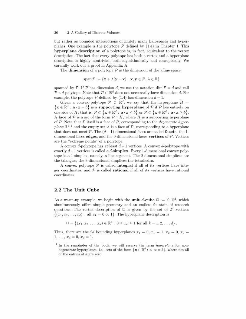
Thus, there are the 2d bounding hyperplanes x1 = 0, x1 = 1, x2 = 0, x2 =1, . . . , xd = 0, xd = 1.
1 In the remainder of the book, we will reserve the term hyperplane for non-degenerate hyperplanes, i.e., sets of the form
˘x ∈ Rd : a · x = b
¯, where not all
of the entries of a are zero.

2.2 The Unit Cube 27
We now compute the discrete volume of any integer dilate of 2. That is,we seek the number of integer points t2∩Zd for all t ∈ Z>0. Here tP denotesthe dilated polytope
{(tx1, tx2, . . . , txd) : (x1, x2, . . . , xd) ∈ P} ,
for any polytope P. What is the discrete volume of 2? We dilate by thepositive integer t, as depicted in Figure 2.1, and count:
#(t2 ∩ Zd
)= #
([0, t]d ∩ Zd
)= (t+ 1)d.
x1
x2
6
6
Fig. 2.1. The sixth dilate of 2 in dimension 2.
We generally denote the lattice-point enumerator for the tth dilates ofP ⊂ Rd by
LP(t) := #(tP ∩ Zd
),
a useful object that we also call the discrete volume of P. We may alsothink of leaving P fixed and shrinking the integer lattice:
LP(t) = #(P ∩ 1
tZd).
With this convention, L2(t) = (t+ 1)d, a polynomial in the integer variable t.Notice that the coefficients of this polynomial are the binomial coefficients(dk
), defined through(
m
n
):=
m(m− 1)(m− 2) · · · (m− n+ 1)n!
(2.1)
for m ∈ C, n ∈ Z>0.
28 2 A Gallery of Discrete Volumes
What about the interior 2◦ of the cube? The number of interior integerpoints in t2◦ is
L2◦(t) = #(t2◦ ∩ Zd
)= #
((0, t)d ∩ Zd
)= (t− 1)d.
Notice that this polynomial equals (−1)dL2(−t), the evaluation of the poly-nomial L2(t) at negative integers, up to a sign.
We now introduce another important tool for analyzing any polytope P,namely the generating function of LP :
EhrP(z) := 1 +∑t≥1
LP(t) zt.
This generating function is also called the Ehrhart series of P.In our case, the Ehrhart series of P = 2 takes on a special form. To
illustrate, we define the Eulerian number A (d, k) through
∑j≥0
jd zj =∑dk=0A (d, k) zk
(1− z)d+1. (2.2)
It is not hard to prove that the polynomial∑dk=1A (d, k) zk is the numerator
of the rational function(zd
dz
)d( 11− z
)= z
d
dz· · · z d
dz︸ ︷︷ ︸d times
(1
1− z
).
The Eulerian numbers have many fascinating properties, including
A (d, k) = A (d, d+ 1− k) ,A (d, k) = (d− k + 1)A (d− 1, k − 1) + k A (d− 1, k) ,
d∑k=0
A (d, k) = d! , (2.3)
A (d, k) =k∑j=0
(−1)j(d+ 1j
)(k − j)d.
The first few Eulerian numbers A (d, k) for 0 ≤ k ≤ d are
d = 0: 1d = 1: 0 1d = 2: 0 1 1d = 3: 0 1 4 1d = 4: 0 1 11 11 1d = 5: 0 1 26 66 26 1d = 6: 0 1 57 302 302 57 1 .
2.3 The Standard Simplex 29
(See also [165, Sequence A008292].)With this definition, we can now express the Ehrhart series of 2 in terms
of Eulerian numbers:
Ehr2(z) = 1 +∑t≥1
(t+ 1)d zt =∑t≥0
(t+ 1)d zt =1z
∑t≥1
td zt
=∑dk=1A (d, k) zk−1
(1− z)d+1.
To summarize, we have proved the following theorem.
Theorem 2.1. Let 2 be the unit d-cube.
(a) The lattice-point enumerator of 2 is the polynomial
L2(t) = (t+ 1)d =d∑k=0
(d
k
)tk.
(b) Its evaluation at negative integers yields the relation
(−1)dL2(−t) = L2◦(t) .
(c) The Ehrhart series of 2 is Ehr2(z) =Pdk=1 A(d,k)zk−1
(1−z)d+1 . ut
2.3 The Standard Simplex
The standard simplex ∆ in dimension d is the convex hull of the d + 1points e1, e2, . . . , ed and the origin; here ej is the unit vector (0, . . . , 1, . . . , 0),with a 1 in the jth position. Figure 2.2 shows ∆ for d = 3. On the other hand,∆ can also be realized by its hyperplane description, namely
∆ ={
(x1, x2 . . . , xd) ∈ Rd : x1 + x2 + · · ·+ xd ≤ 1 and all xk ≥ 0}.
In the case of the standard simplex, the dilate t∆ is now given by
t∆ ={
(x1, x2, . . . , xd) ∈ Rd : x1 + x2 + · · ·+ xd ≤ t and all xk ≥ 0}.
To compute the discrete volume of ∆, we would like to use the methods devel-oped in Chapter 1, but there’s an extra twist. The counting functions in Chap-ter 1 were defined by equalities, whereas the standard simplex is defined by aninequality. We are trying to count all integer solutions (m1,m2, . . . ,md) ∈ Zd≥0
tom1 +m2 + · · ·+md ≤ t . (2.4)
To translate this inequality in d variables into an equality in d + 1 vari-ables, we introduce a slack variable md+1 ∈ Z≥0, which picks up the dif-ference between the right-hand and left-hand sides of (2.4). So the number
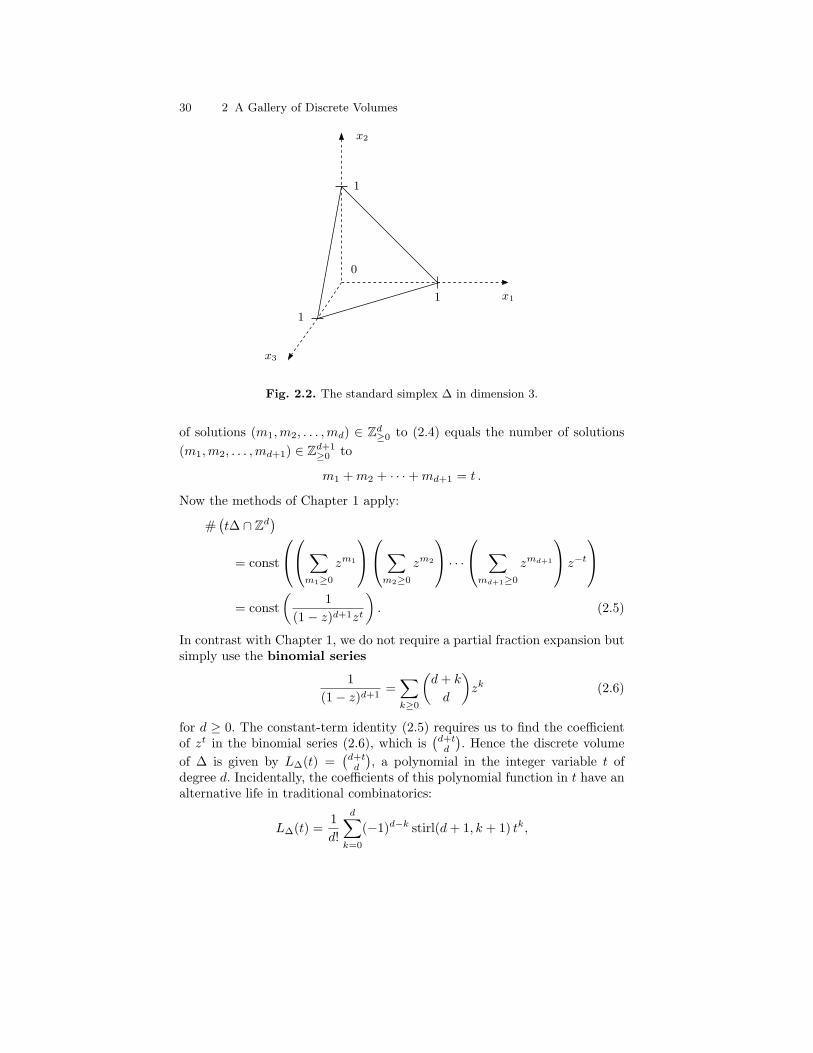
30 2 A Gallery of Discrete Volumes
x1
x2
x3
0
1
1
1
Fig. 2.2. The standard simplex ∆ in dimension 3.
of solutions (m1,m2, . . . ,md) ∈ Zd≥0 to (2.4) equals the number of solutions(m1,m2, . . . ,md+1) ∈ Zd+1
≥0 to
m1 +m2 + · · ·+md+1 = t .
Now the methods of Chapter 1 apply:
#(t∆ ∩ Zd
)= const
∑m1≥0
zm1
∑m2≥0
zm2
· · · ∑md+1≥0
zmd+1
z−t
= const
(1
(1− z)d+1zt
). (2.5)
In contrast with Chapter 1, we do not require a partial fraction expansion butsimply use the binomial series
1(1− z)d+1
=∑k≥0
(d+ k
d
)zk (2.6)
for d ≥ 0. The constant-term identity (2.5) requires us to find the coefficientof zt in the binomial series (2.6), which is
(d+td
). Hence the discrete volume
of ∆ is given by L∆(t) =(d+td
), a polynomial in the integer variable t of
degree d. Incidentally, the coefficients of this polynomial function in t have analternative life in traditional combinatorics:
L∆(t) =1d!
d∑k=0
(−1)d−k stirl(d+ 1, k + 1) tk,
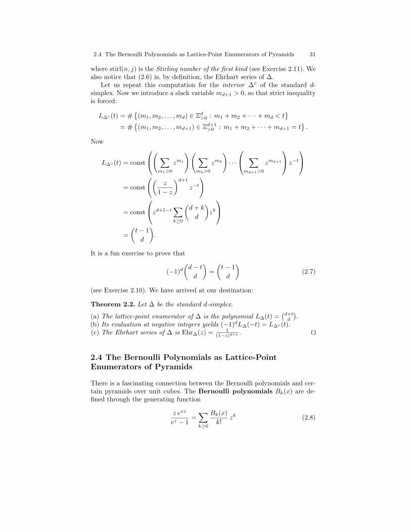
2.4 The Bernoulli Polynomials as Lattice-Point Enumerators of Pyramids 31
where stirl(n, j) is the Stirling number of the first kind (see Exercise 2.11). Wealso notice that (2.6) is, by definition, the Ehrhart series of ∆.
Let us repeat this computation for the interior ∆◦ of the standard d-simplex. Now we introduce a slack variable md+1 > 0, so that strict inequalityis forced:
L∆◦(t) = #{
(m1,m2, . . . ,md) ∈ Zd>0 : m1 +m2 + · · ·+md < t}
= #{
(m1,m2, . . . ,md+1) ∈ Zd+1>0 : m1 +m2 + · · ·+md+1 = t
}.
Now
L∆◦(t) = const
(∑m1>0
zm1
)( ∑m2>0
zm2
)· · ·
∑md+1>0
zmd+1
z−t
= const
((z
1− z
)d+1
z−t
)
= const
zd+1−t∑k≥0
(d+ k
d
)zk
=(t− 1d
).
It is a fun exercise to prove that
(−1)d(d− td
)=(t− 1d
)(2.7)
(see Exercise 2.10). We have arrived at our destination:
Theorem 2.2. Let ∆ be the standard d-simplex.
(a) The lattice-point enumerator of ∆ is the polynomial L∆(t) =(d+td
).
(b) Its evaluation at negative integers yields (−1)dL∆(−t) = L∆◦(t).(c) The Ehrhart series of ∆ is Ehr∆(z) = 1
(1−z)d+1 . ut
2.4 The Bernoulli Polynomials as Lattice-PointEnumerators of Pyramids
There is a fascinating connection between the Bernoulli polynomials and cer-tain pyramids over unit cubes. The Bernoulli polynomials Bk(x) are de-fined through the generating function
z exz
ez − 1=∑k≥0
Bk(x)k!
zk (2.8)
32 2 A Gallery of Discrete Volumes
and are ubiquitous in the study of the Riemann zeta function, among otherobjects; they are named after Jacob Bernoulli (1654–1705).2 The Bernoullipolynomials will play a prominent role in Chapter 10 in the context of Euler–Maclaurin summation. The first few Bernoulli polynomials are
B0(x) = 1 ,
B1(x) = x− 12,
B2(x) = x2 − x+16,
B3(x) = x3 − 32x2 +
12x ,
B4(x) = x4 − 2x3 + x2 − 130,
B5(x) = x5 − 52x4 +
53x3 − 1
6x ,
B6(x) = x6 − 3x5 +52x4 +
12x2 +
142,
B7(x) = x7 − 72x6 +
72x5 +
76x3 +
16x .
The Bernoulli numbers are Bk := Bk(0) (see also [165, Sequences A000367& A002445]) and have the generating function
z
ez − 1=∑k≥0
Bkk!
zk.
Lemma 2.3. For integers d ≥ 1 and n ≥ 2,
n−1∑k=0
kd−1 =1d
(Bd(n)−Bd) .
Proof. We play with the generating function of Bd(n)−Bdd! :
∑d≥0
Bd(n)−Bdd!
zd = zenz − 1ez − 1
= z
n−1∑k=0
ekz = z
n−1∑k=0
∑j≥0
(kz)j
j!
=∑j≥0
(n−1∑k=0
kj
)zj+1
j!=∑j≥1
(n−1∑k=0
kj−1
)zj
(j − 1)!.
Now compare coefficients on both sides. ut
2 For more information about Bernoulli, seehttp://www-groups.dcs.st-and.ac.uk/∼history/Mathematicians/Bernoulli Jacob.html.
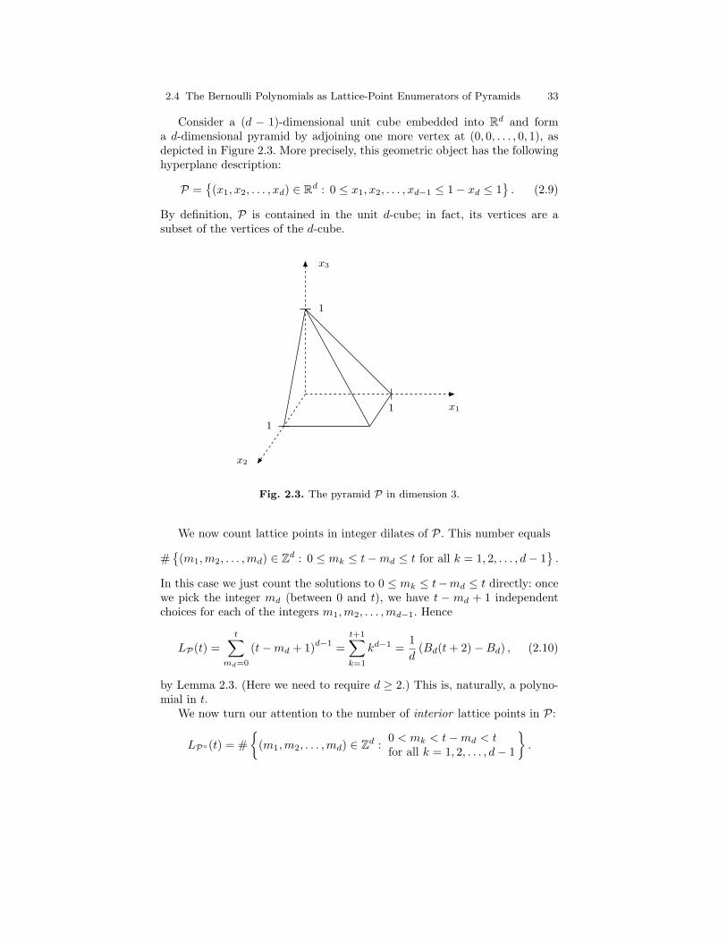
2.4 The Bernoulli Polynomials as Lattice-Point Enumerators of Pyramids 33
Consider a (d − 1)-dimensional unit cube embedded into Rd and forma d-dimensional pyramid by adjoining one more vertex at (0, 0, . . . , 0, 1), asdepicted in Figure 2.3. More precisely, this geometric object has the followinghyperplane description:
P ={
(x1, x2, . . . , xd) ∈ Rd : 0 ≤ x1, x2, . . . , xd−1 ≤ 1− xd ≤ 1}. (2.9)
By definition, P is contained in the unit d-cube; in fact, its vertices are asubset of the vertices of the d-cube.
x1
x3
x2
1
1
1
Fig. 2.3. The pyramid P in dimension 3.
We now count lattice points in integer dilates of P. This number equals
#{
(m1,m2, . . . ,md) ∈ Zd : 0 ≤ mk ≤ t−md ≤ t for all k = 1, 2, . . . , d− 1}.
In this case we just count the solutions to 0 ≤ mk ≤ t−md ≤ t directly: oncewe pick the integer md (between 0 and t), we have t −md + 1 independentchoices for each of the integers m1,m2, . . . ,md−1. Hence
LP(t) =t∑
md=0
(t−md + 1)d−1 =t+1∑k=1
kd−1 =1d
(Bd(t+ 2)−Bd) , (2.10)
by Lemma 2.3. (Here we need to require d ≥ 2.) This is, naturally, a polyno-mial in t.
We now turn our attention to the number of interior lattice points in P:
LP◦(t) = #{
(m1,m2, . . . ,md) ∈ Zd :0 < mk < t−md < tfor all k = 1, 2, . . . , d− 1
}.

34 2 A Gallery of Discrete Volumes
By a similar counting argument,
LP◦(t) =t−1∑md=1
(t−md − 1)d−1 =t−2∑k=0
kd−1 =1d
(Bd(t− 1)−Bd) .
Incidentally, the Bernoulli polynomials are known (Exercise 2.15) to have thesymmetry
Bd(1− x) = (−1)dBd(x) . (2.11)
This identity coupled with the fact (Exercise 2.16) that
Bd = 0 for all odd d ≥ 3 (2.12)
gives the relation
LP(−t) =1d
(Bd(−t+ 2)−Bd) =1d
(Bd (1− (t− 1))−Bd)
= (−1)d1d
(Bd(t− 1)−Bd) = (−1)d LP◦(t) .
Next we compute the Ehrhart series of P. We can actually do this insomewhat greater generality. Namely, for a (d − 1)-polytope Q with verticesv1,v2, . . . ,vm, define Pyr(Q), the pyramid over Q, as the convex hull of(v1, 0) , (v2, 0) , . . . , (vm, 0) , (0, . . . , 0, 1). In our example above, the d-polytopeP is equal to Pyr(2) for the unit (d−1)-cube 2. The number of integer pointsin tPyr(Q) is, by construction,
LPyr(Q)(t) = 1 + LQ(1) + LQ(2) + · · ·+ LQ(t) = 1 +t∑
j=1
LQ(j) ,
because in tPyr(Q), there is one lattice point with xd-coordinate t, LQ(1)lattice points with xd-coordinate t−1, LQ(2) lattice points with xd-coordinatet−2, etc., up to LQ(t) lattice points with xd = 0. Figure 2.4 shows the instancet = 3 for a pyramid over a square.
This identity for LPyr(Q)(t) allows us to compute the Ehrhart series ofPyr(Q) from the Ehrhart series of Q:
Theorem 2.4. EhrPyr(Q)(z) =EhrQ(z)
1− z.
Proof.
EhrPyr(Q)(z) = 1 +∑t≥1
LPyr(Q)(t) zt = 1 +∑t≥1
1 +t∑
j=1
LQ(j)
zt
=∑t≥0
zt +∑t≥1
t∑j=1
LQ(j) zt =1
1− z+∑j≥1
LQ(j)∑t≥j
zt
=1
1− z+∑j≥1
LQ(j)zj
1− z=
1 +∑j≥1 LQ(j) zj
1− z. ut

2.5 The Lattice-Point Enumerators of the Cross-Polytopes 35
x1
x3
x2
Fig. 2.4. Counting the lattice points in tPyr(Q).
Our pyramid P that started this section is a pyramid over the unit (d−1)-cube, and so
EhrP(z) =1
1− z
∑d−1k=1A (d− 1, k) zk−1
(1− z)d=∑d−1k=1A (d− 1, k) zk−1
(1− z)d+1. (2.13)
Let’s summarize what we have proved for the pyramid over the unit cube.
Theorem 2.5. Given d ≥ 2, let P be the d-pyramid
P ={
(x1, x2, . . . , xd) ∈ Rd : 0 ≤ x1, x2, . . . , xd−1 ≤ 1− xd ≤ 1}.
(a) The lattice-point enumerator of P is the polynomial
LP(t) =1d
(Bd(t+ 2)−Bd) .
(b) Its evaluation at negative integers yields (−1)dLP(−t) = LP◦(t).
(c) The Ehrhart series of P is EhrP(z) =Pd−1k=1 A(d−1,k)zk−1
(1−z)d+1 . ut
Patterns are emerging...
2.5 The Lattice-Point Enumerators of theCross-Polytopes
Consider the cross-polytope 3 in Rd given by the hyperplane description

36 2 A Gallery of Discrete Volumes
3 :={
(x1, x2, . . . , xd) ∈ Rd : |x1|+ |x2|+ · · ·+ |xd| ≤ 1}. (2.14)
Figure 2.5 shows the 3-dimensional instance of 3, an octahedron. The verticesof 3 are (±1, 0, . . . , 0) , (0,±1, 0, . . . , 0) , . . . , (0, . . . , 0,±1).
x1
x2
x3
Fig. 2.5. The cross-polytope 3 in dimension 3.
To compute the discrete volume of 3, we use a process similar to that ofSection 2.4. Namely, for a (d − 1)-polytope Q with vertices v1,v2, . . . ,vm,such that the origin is in Q, define BiPyr(Q), the bipyramid over Q, as theconvex hull of
(v1, 0) , (v2, 0) , . . . , (vm, 0) , (0, . . . , 0, 1) , and (0, . . . , 0,−1) .
In our example above, the d-dimensional cross-polytope is the bipyramidover the (d− 1)-dimensional cross-polytope. The number of integer points intBiPyr(Q) is, by construction,
LBiPyr(Q)(t) = 2 + 2LQ(1) + 2LQ(2) + · · ·+ 2LQ(t− 1) + LQ(t)
= 2 + 2t−1∑j=1
LQ(j) + LQ(t) .
This identity allows us to compute the Ehrhart series of BiPyr(Q) from theEhrhart series of Q, in a manner similar to the proof of Theorem 2.4. We leavethe proof of the following result as Exercise 2.23.
Theorem 2.6. If Q contains the origin, then EhrBiPyr(Q)(z) = 1+z1−z EhrQ(z).
ut

2.5 The Lattice-Point Enumerators of the Cross-Polytopes 37
This theorem allows us to compute the Ehrhart series of 3 effortlessly:The cross-polytope 3 in dimension 0 is the origin, with Ehrhart series 1
1−z .The higher-dimensional cross-polytopes can be computed recursively throughTheorem 2.6 as
Ehr3(z) =(1 + z)d
(1− z)d+1.
Since Ehr3(z) = 1 +∑t≥1 L3(t) zt, we can retrieve L3(t) by expanding
Ehr3(z) into its power series at z = 0:
Ehr3(z) =(1 + z)d
(1− z)d+1=∑dk=0
(dk
)zk
(1− z)d+1
=d∑k=0
(d
k
)zk∑t≥0
(t+ d
d
)zt =
d∑k=0
(d
k
)∑t≥k
(t− k + d
d
)zt
=d∑k=0
(d
k
)∑t≥0
(t− k + d
d
)zt.
In the last step we used the fact that(t−k+dd
)= 0 for 0 ≤ t < k. But then
1 +∑t≥1
L3(t) zt =∑t≥0
d∑k=0
(d
k
)(t− k + d
d
)zt,
and hence L3(t) =∑dk=0
(dk
)(t−k+dd
)for all t ≥ 1.
We finish this section by counting the interior lattice points in t3. Westart by noticing, since t is an integer, that
L3◦(t) = #{
(m1,m2, . . . ,md) ∈ Zd : |m1|+ |m2|+ · · ·+ |md| < t}
= #{
(m1,m2, . . . ,md) ∈ Zd : |m1|+ |m2|+ · · ·+ |md| ≤ t− 1}
= L3(t− 1) .
On the other hand, we can use (2.7):
L3(−t) =d∑k=0
(d
k
)(−t− k + d
d
)
=d∑k=0
(d
k
)(−1)d
(t− 1 + k
d
)
= (−1)dd∑k=0
(d
d− k
)(t− 1 + d− k
d
)= (−1)dL3(t− 1) .
Comparing the last two computations, we see that (−1)dL3(−t) = L3◦(t).Let us summarize:
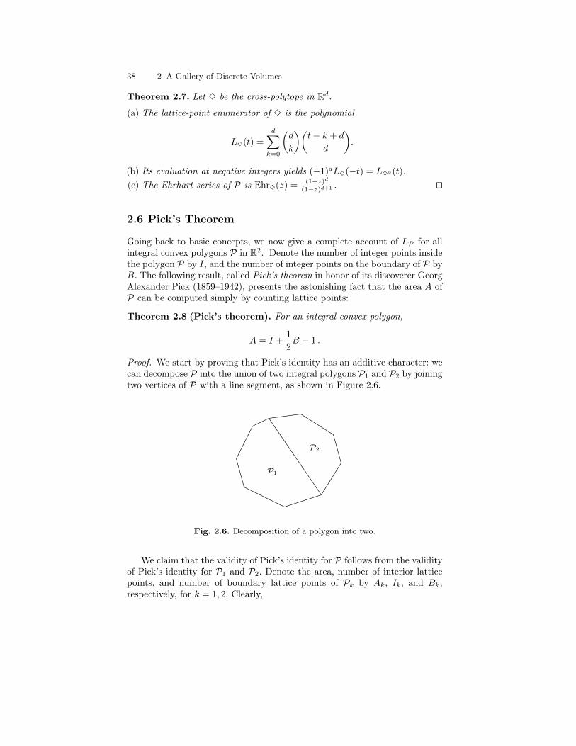
38 2 A Gallery of Discrete Volumes
Theorem 2.7. Let 3 be the cross-polytope in Rd.
(a) The lattice-point enumerator of 3 is the polynomial
L3(t) =d∑k=0
(d
k
)(t− k + d
d
).
(b) Its evaluation at negative integers yields (−1)dL3(−t) = L3◦(t).(c) The Ehrhart series of P is Ehr3(z) = (1+z)d
(1−z)d+1 . ut
2.6 Pick’s Theorem
Going back to basic concepts, we now give a complete account of LP for allintegral convex polygons P in R2. Denote the number of integer points insidethe polygon P by I, and the number of integer points on the boundary of P byB. The following result, called Pick’s theorem in honor of its discoverer GeorgAlexander Pick (1859–1942), presents the astonishing fact that the area A ofP can be computed simply by counting lattice points:
Theorem 2.8 (Pick’s theorem). For an integral convex polygon,
A = I +12B − 1 .
Proof. We start by proving that Pick’s identity has an additive character: wecan decompose P into the union of two integral polygons P1 and P2 by joiningtwo vertices of P with a line segment, as shown in Figure 2.6.
P1
P2
Fig. 2.6. Decomposition of a polygon into two.
We claim that the validity of Pick’s identity for P follows from the validityof Pick’s identity for P1 and P2. Denote the area, number of interior latticepoints, and number of boundary lattice points of Pk by Ak, Ik, and Bk,respectively, for k = 1, 2. Clearly,
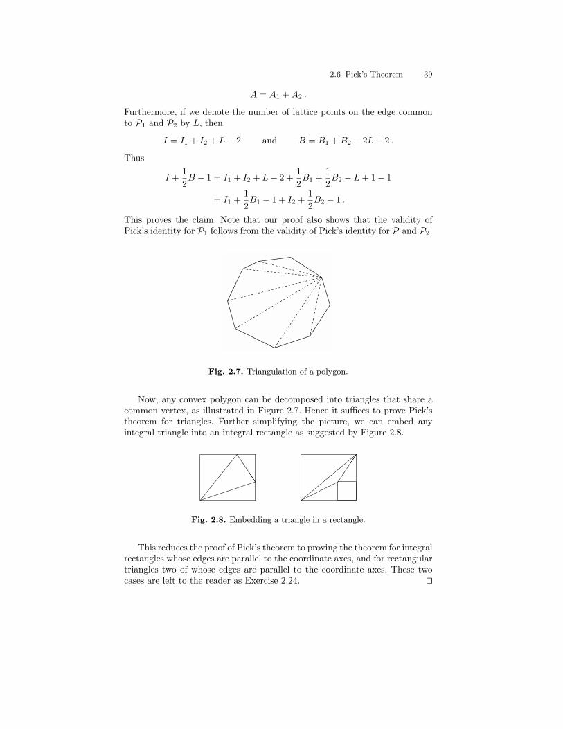
2.6 Pick’s Theorem 39
A = A1 +A2 .
Furthermore, if we denote the number of lattice points on the edge commonto P1 and P2 by L, then
I = I1 + I2 + L− 2 and B = B1 +B2 − 2L+ 2 .
Thus
I +12B − 1 = I1 + I2 + L− 2 +
12B1 +
12B2 − L+ 1− 1
= I1 +12B1 − 1 + I2 +
12B2 − 1 .
This proves the claim. Note that our proof also shows that the validity ofPick’s identity for P1 follows from the validity of Pick’s identity for P and P2.
Fig. 2.7. Triangulation of a polygon.
Now, any convex polygon can be decomposed into triangles that share acommon vertex, as illustrated in Figure 2.7. Hence it suffices to prove Pick’stheorem for triangles. Further simplifying the picture, we can embed anyintegral triangle into an integral rectangle as suggested by Figure 2.8.
�����JJJJ
����
��
,,,,,,
���
�
Fig. 2.8. Embedding a triangle in a rectangle.
This reduces the proof of Pick’s theorem to proving the theorem for integralrectangles whose edges are parallel to the coordinate axes, and for rectangulartriangles two of whose edges are parallel to the coordinate axes. These twocases are left to the reader as Exercise 2.24. ut
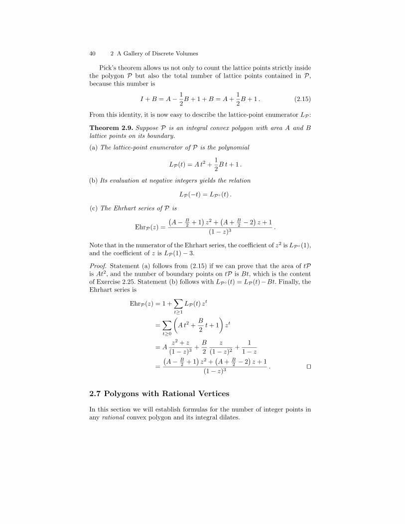
40 2 A Gallery of Discrete Volumes
Pick’s theorem allows us not only to count the lattice points strictly insidethe polygon P but also the total number of lattice points contained in P,because this number is
I +B = A− 12B + 1 +B = A+
12B + 1 . (2.15)
From this identity, it is now easy to describe the lattice-point enumerator LP :
Theorem 2.9. Suppose P is an integral convex polygon with area A and Blattice points on its boundary.
(a) The lattice-point enumerator of P is the polynomial
LP(t) = A t2 +12B t+ 1 .
(b) Its evaluation at negative integers yields the relation
LP(−t) = LP◦(t) .
(c) The Ehrhart series of P is
EhrP(z) =
(A− B
2 + 1)z2 +
(A+ B
2 − 2)z + 1
(1− z)3.
Note that in the numerator of the Ehrhart series, the coefficient of z2 is LP◦(1),and the coefficient of z is LP(1)− 3.
Proof. Statement (a) follows from (2.15) if we can prove that the area of tPis At2, and the number of boundary points on tP is Bt, which is the contentof Exercise 2.25. Statement (b) follows with LP◦(t) = LP(t)−Bt. Finally, theEhrhart series is
EhrP(z) = 1 +∑t≥1
LP(t) zt
=∑t≥0
(A t2 +
B
2t+ 1
)zt
= Az2 + z
(1− z)3+B
2z
(1− z)2+
11− z
=
(A− B
2 + 1)z2 +
(A+ B
2 − 2)z + 1
(1− z)3. ut
2.7 Polygons with Rational Vertices
In this section we will establish formulas for the number of integer points inany rational convex polygon and its integral dilates.

2.7 Polygons with Rational Vertices 41
A natural first step is to fix a triangulation of the polygon P, which reducesour problem to that of counting integer points in rational triangles. However,this procedure merits some remarks. After counting lattice points in the tri-angles, we need to put those back together to form the polygon. But then weneed to take care of the overcounting on line segments (where the trianglesmeet). Computing the number of lattice points on rational line segments isconsiderably easier than enumerating lattice points in 2-dimensional regions;however, it is still nontrivial (see Popoviciu’s Theorem 1.5).
After triangulating P, we can further simplify the picture by embedding anarbitrary rational triangle in a rational rectangle as in Figure 2.8. To computelattice points in a triangle, we can first count the points in a rectangle withedges parallel to the coordinate axes, and then subtract the number of pointsin three right triangles, each with two edges are parallel to the axes, andpossibly another rectangle, as shown in Figure 2.8. Since rectangles are easyto deal with (see Exercise 2.2), the problem reduces to finding a formula fora right triangle two of whose edges are parallel to the coordinate axes.
We now adjust and expand our generating-function machinery to theseright triangles. Such a triangle T is a subset of R2 consisting of all points(x, y) satisfying
x ≥ a
d, y ≥ b
d, ex+ fy ≤ r
for some integers a, b, d, e, f, r (with ea+fb ≤ rd; otherwise, the triangle wouldbe empty). Because the lattice point count is invariant under horizontal andvertical integer translations and under flipping about the x- or y-axis, we mayassume that a, b, d, e, f, r ≥ 0 and a, b < d. (One should meditate about thisfact for a minute.) Thus we arrive at the triangle T depicted in Figure 2.9.
x
y
„r − fb/d
e,b
d
«„a
d,b
d
«
„a
d,r − ea/d
f
«
Fig. 2.9. A right rational triangle.
42 2 A Gallery of Discrete Volumes
To make our life a little easier, let’s assume for the moment that e and fare relatively prime; we will deal with the general case in the exercises. So let
T ={
(x, y) ∈ R2 : x ≥ a
d, y ≥ b
d, ex+ fy ≤ r
}. (2.16)
To derive a formula for
LT (t) = #{
(m,n) ∈ Z2 : m ≥ ta
d, n ≥ tb
d, em+ fn ≤ tr
}we want to use methods similar to those in Chapter 1. As in Section 2.3, weintroduce a slack variable s:
LT (t) = #{
(m,n) ∈ Z2 : m ≥ ta
d, n ≥ tb
d, em+ fn ≤ tr
}= #
{(m,n, s) ∈ Z3 : m ≥ ta
d, n ≥ tb
d, s ≥ 0, em+ fn+ s = tr
}.
This counting function can now, as earlier, be interpreted as the coefficient ofztr in the function ∑
m≥ tad
zem
∑n≥ tbd
zfn
∑s≥0
zs
.
Here the subscript (e.g., m ≥ tad ) under a summation sign means “sum over
all integers satisfying this condition.” For example, in the first sum we startwith the least integer greater than or equal to ta
d , which is denoted by⌈tad
⌉(and is equal to
⌊ta−1d
⌋+ 1 by Exercise 1.4 (j)). Hence the above generating
function can be rewritten as ∑m≥d tad e
zem
∑n≥d tbd e
zfn
∑s≥0
zs
=zd
tad ee
1− zezd
tbd ef
1− zf1
1− z
=zu+v
(1− ze) (1− zf ) (1− z), (2.17)
where we have introduced, for ease of notation,
u :=⌈ta
d
⌉e and v :=
⌈tb
d
⌉f . (2.18)
To extract the coefficient of ztr of our generating function (2.17), we usefamiliar methods. As usual, we shift this coefficient to a constant term:
LT (t) = const(
zu+v−tr
(1− ze) (1− zf ) (1− z)
)= const
(1
(1− ze) (1− zf ) (1− z)ztr−u−v
).
2.7 Polygons with Rational Vertices 43
Before we apply the partial fraction machinery to this function, we shouldmake sure that it is indeed a proper rational function, that is, that the totaldegree satisfies
u+ v − tr − e− f − 1 < 0 (2.19)
(see Exercise 2.31). Then we expand into partial fractions (here we’re usingour assumption that e and f do not have any common factors!):
1(1− ze) (1− zf ) (1− z)ztr−u−v
=e−1∑j=1
Aj
z − ξje+f−1∑j=1
Bj
z − ξjf+
3∑k=1
Ck(z − 1)k
+tr−u−v∑k=1
Dk
zk. (2.20)
As numerous times before, the coefficients Dk do not contribute to the con-stant term, so that we obtain
LT (t) = −e−1∑j=1
Aj
ξje−f−1∑l=1
Blξlf− C1 + C2 − C3 . (2.21)
We invite the reader to compute the coefficients appearing in this formula(Exercise 2.32):
Aj = − ξj(v−tr+1)e
e(
1− ξjfe)
(1− ξje),
Bl = −ξl(u−tr+1)f
f(
1− ξlef)
(1− ξlf ),
C1 = − (u+ v − tr)2
2ef+u+ v − tr
2
(− 1ef
+1e
+1f
)+
14
(1e
+1f− 1)
− 112
(e
f+
1ef
+f
e
), (2.22)
C2 = −u+ v − tr + 1ef
+12e
+1
2f,
C3 = − 1ef
.
Putting these ingredients into (2.21) yields the following formula for ourlattice-point count.
Theorem 2.10. For the rectangular rational triangle T given by (2.16), wheree and f are relatively prime,

44 2 A Gallery of Discrete Volumes
LT (t) =1
2ef(tr − u− v)2 +
12
(tr − u− v)(
1e
+1f
+1ef
)+
14
(1 +
1e
+1f
)+
112
(e
f+f
e+
1ef
)+
1e
e−1∑j=1
ξj(v−tr)e(
1− ξjfe)(
1− ξje) +
1f
f−1∑l=1
ξl(u−tr)f(
1− ξlef)(
1− ξlf) . ut
This identity can be rephrased in terms of the Fourier–Dedekind sum thatwe introduced in (1.13):
LT (t) =1
2ef(tr − u− v)2 +
12
(tr − u− v)(
1e
+1f
+1ef
)+
14
(1 +
1e
+1f
)+
112
(e
f+f
e+
1ef
)+ sv−tr(f, 1; e) + su−tr(e, 1; f) .
The general formula for LT—not assuming that e and f are relativelyprime—is the content of Exercise 2.34.
Let us pause for a moment and study the nature of LT as a functionof t. Aside from the last two finite sums (which will be put in the spotlightin Chapter 8) and the appearance of u and v, LT is a quadratic polynomialin t. And in those two sums, t appears only in the exponent of roots of unity,namely as the exponent of ξe and ξf . As a function of t, ξte is periodic withperiod e, and similarly ξtf is periodic with period f . We should also rememberthat u and v are functions of t; but they can be easily written in terms ofthe fractional-part function, which again gives rise to periodic functions in t.So LT (t) is a (quadratic) “polynomial” in t, whose coefficients are periodicfunctions in t. This is reminiscent of the counting functions of Chapter 1, whichshowed a similar periodic-polynomial behavior. Inspired by both examples, wedefine a quasipolynomial Q as an expression of the form Q(t) = cn(t) tn +· · ·+ c1(t) t+ c0(t), where c0, . . . , cn are periodic functions in t. The degreeof Q is n,3 and the least common period of c0, . . . , cn is the period of Q.Alternatively, for a quasipolynomial Q, there exist a positive integer k andpolynomials p0, p1, . . . , pk−1 such that
Q(t) =
p0(t) if t ≡ 0 mod k,
p1(t) if t ≡ 1 mod k,...
pk−1(t) if t ≡ k − 1 mod k.
The minimal such k is the period of Q, and for this minimal k, the polynomialsp0, p1, . . . , pk−1 are the constituents of Q.3 Here we tacitly assume that cn is not the zero function.

2.8 Euler’s Generating Function for General Rational Polytopes 45
By the triangulation and embedding-in-a-box arguments that started thissection, we can now state a general structural result for rational polygons.
Theorem 2.11. Let P be any rational polygon. Then LP(t) is a quasipolyno-mial of degree 2. Its leading coefficient is the area of P (in particular, it is aconstant).
We have the technology at this point to also study the period of LP ; welet the reader enjoy the ensuing details (see Exercise 2.35).
Proof. By Exercises 2.2 and 2.34 (the general form of Theorem 2.10), the the-orem holds for rational rectangles and right triangles whose edges are parallelto the axes. Now use the additivity of both degree-2 quasipolynomials andareas, and Popoviciu’s theorem (Theorem 1.5). ut
2.8 Euler’s Generating Function for General RationalPolytopes
By now we have computed several instances of counting functions by set-ting up a generating function that fits the particular problem we’re interestedin. In this section, we set up such a generating function for the lattice-pointenumerator of any rational polytope. Such a polytope is given by its hyper-plane description as an intersection of half-spaces and hyperplanes. The half-spaces are algebraically given by linear inequalities, the hyperplanes by linearequations. If the polytope is rational, we can choose the coefficients of theseinequalities and equations to be integers (Exercise 2.7). To unify both de-scriptions, we can introduce slack variables to turn the half-space inequalitiesinto equalities. Furthermore, by translating our polytope into the nonnegativeorthant (we can always shift a polytope by an integer vector without changingthe lattice-point count), we may assume that all points in the polytope havenonnegative coordinates. In summary, after a harmless integer translation, wecan describe any rational polytope P as
P ={x ∈ Rd≥0 : A x = b
}(2.23)
for some integral matrix A ∈ Zm×d and some integer vector b ∈ Zm. (Notethat d is not necessarily the dimension of P.) To describe the tth dilate of P,we simply scale a point x ∈ P by 1
t , or alternatively, multiply b by t:
tP ={
x ∈ Rd≥0 : Axt
= b}
={x ∈ Rd≥0 : A x = tb
}.
Hence the lattice-point enumerator of P is the counting function
LP(t) = #{x ∈ Zd≥0 : A x = tb
}. (2.24)
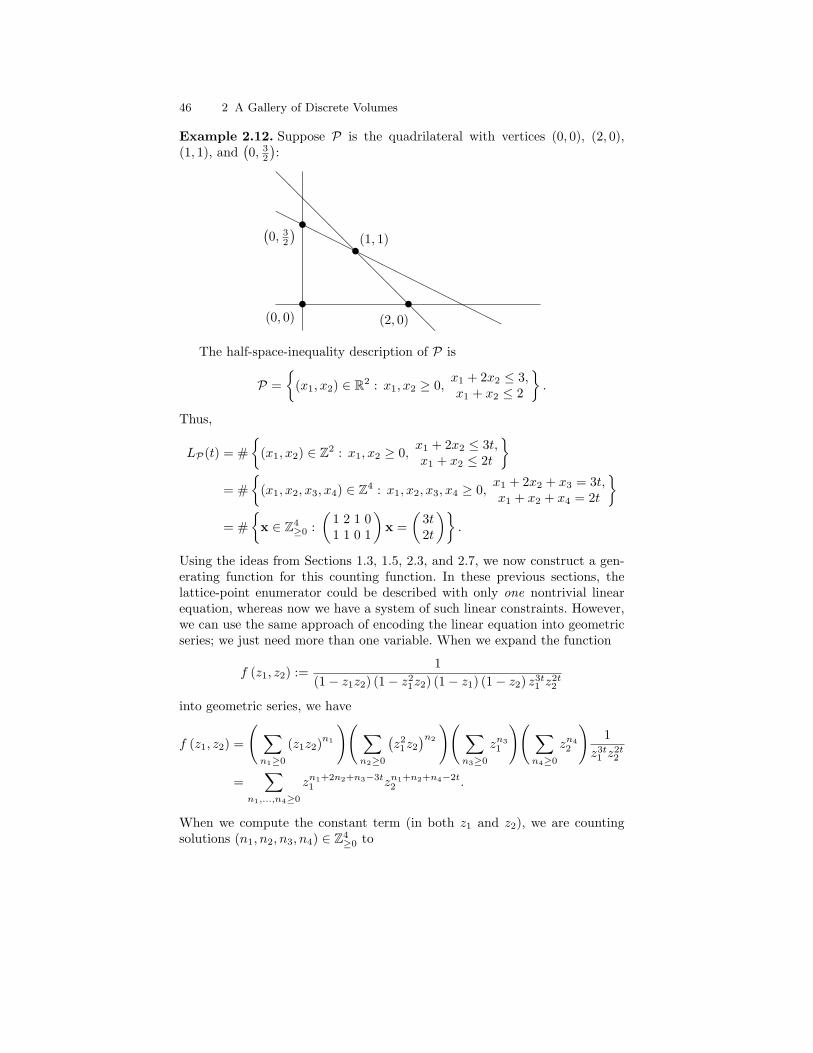
46 2 A Gallery of Discrete Volumes
Example 2.12. Suppose P is the quadrilateral with vertices (0, 0), (2, 0),(1, 1), and
(0, 3
2
):
@@@@@@@@@@@@
HHHHHH
HHHHHH
HHHHH
t(0, 3
2
)
t(2, 0)
t(1, 1)
t(0, 0)
The half-space-inequality description of P is
P ={
(x1, x2) ∈ R2 : x1, x2 ≥ 0,x1 + 2x2 ≤ 3,x1 + x2 ≤ 2
}.
Thus,
LP(t) = #{
(x1, x2) ∈ Z2 : x1, x2 ≥ 0,x1 + 2x2 ≤ 3t,x1 + x2 ≤ 2t
}= #
{(x1, x2, x3, x4) ∈ Z4 : x1, x2, x3, x4 ≥ 0,
x1 + 2x2 + x3 = 3t,x1 + x2 + x4 = 2t
}= #
{x ∈ Z4
≥0 :(
1 2 1 01 1 0 1
)x =
(3t2t
)}.
Using the ideas from Sections 1.3, 1.5, 2.3, and 2.7, we now construct a gen-erating function for this counting function. In these previous sections, thelattice-point enumerator could be described with only one nontrivial linearequation, whereas now we have a system of such linear constraints. However,we can use the same approach of encoding the linear equation into geometricseries; we just need more than one variable. When we expand the function
f (z1, z2) :=1
(1− z1z2) (1− z21z2) (1− z1) (1− z2) z3t
1 z2t2
into geometric series, we have
f (z1, z2) =
( ∑n1≥0
(z1z2)n1
)( ∑n2≥0
(z2
1z2
)n2
)( ∑n3≥0
zn31
)( ∑n4≥0
zn42
)1
z3t1 z
2t2
=∑
n1,...,n4≥0
zn1+2n2+n3−3t1 zn1+n2+n4−2t
2 .
When we compute the constant term (in both z1 and z2), we are countingsolutions (n1, n2, n3, n4) ∈ Z4
≥0 to

2.8 Euler’s Generating Function for General Rational Polytopes 47
(1 2 1 01 1 0 1
)n1
n2
n3
n4
=(
3t2t
),
that is, the constant term of f (z1, z2) counts the integer points in P:
LP(t) = const1
(1− z1z2) (1− z21z2) (1− z1) (1− z2) z3t
1 z2t2
.
We invite the reader to actually compute this constant term (Exercise 2.36).It turns out to be
74t2 +
52t+
7 + (−1)t
8. ut
Returning to the general case of a polytope P given by (2.23), we denotethe columns of A by c1, c2, . . . , cd. Let z = (z1, z2, . . . , zm) and expand thefunction
1(1− zc1) (1− zc2) · · · (1− zcd) ztb
(2.25)
in terms of geometric series:∑n1≥0
zn1c1
∑n2≥0
zn2c2
· · ·∑nd≥0
zndcd
1ztb
.
Here we use the abbreviating notation zc := zc11 zc22 · · · zcmm for the vectors
z = (z1, z2, . . . , zm) ∈ Cm and c = (c1, c2, . . . , cm) ∈ Zm. When multiplyingout everything, a typical exponent will look like
n1c1 + n2c2 + · · ·+ ndcd − tb = An− tb ,
where n = (n1, n2, . . . , nd) ∈ Zd≥0. That is, if we take the constant term of ourgenerating function (2.25), we’re counting integer vectors n ∈ Zd≥0 satisfying
An− tb = 0 , that is, An = tb .
So this constant term will pick up exactly the number of lattice points n ∈ Zd≥0
in tP:
Theorem 2.13 (Euler’s generating function). Suppose the rational poly-tope P is given by (2.23). Then the the lattice-point enumerator of P can becomputed as follows:
LP(t) = const(
1(1− zc1) (1− zc2) · · · (1− zcd) ztb
). ut
We finish this section with rephrasing this constant-term identity in termsof Ehrhart series.

48 2 A Gallery of Discrete Volumes
Corollary 2.14. Suppose the rational polytope P is given by (2.23). Then theEhrhart series of P can be computed as
EhrP(x) = const
(1
(1− zc1) (1− zc2) · · · (1− zcd)(1− x
zb
)) .Proof. By Theorem 2.13,
EhrP(x) =∑t≥0
const(
1(1− zc1) (1− zc2) · · · (1− zcd) ztb
)xt
= const
1(1− zc1) (1− zc2) · · · (1− zcd)
∑t≥0
xt
ztb
= const
(1
(1− zc1) (1− zc2) · · · (1− zcd)1
1− xzb
). ut
Notes
1. Convex polytopes are beautiful objects with a rich history and interest-ing theory, which we have only glimpsed here. For a good introduction topolytopes, we recommend [47, 90, 193]. Polytopes appear in a vast rangeof current research areas, including Grobner bases and commutative algebra[174], combinatorial optimization [159], integral geometry [110], and geometryof numbers [163].
2. The distinction between the vertex and hyperplane description of a convexpolytope leads to an interesting algorithmic question; namely, how quickly canwe retrieve the first piece of data from the second and vice versa [159, 193]?
3. Ehrhart series are named after Eugene Ehrhart (1906–2000),4 in antici-pation of the theorems we will prove in Chapter 3. The Ehrhart series of apolytope belonging to the special class of normal polytopes equals anotherrational generating function, the Hilbert–Poincare series. These series appearin the study of graded algebras (see, for example, [96, 171]). Ehrhart series alsoappear in the context of toric varieties, a vast and fruitful subject [64, 84].
4. The Eulerian numbers A (d, k) are named after Leonhard Euler (1707–1783)5 and arise naturally in the statistics of permutations: A (d, k) countspermutations of {1, 2, . . . , d} with k− 1 ascents. For more on A (d, k), see [62,Section 6.5].4 For more information about Ehrhart, seehttp://icps.u-strasbg.fr/∼clauss/Ehrhart.html.
5 For more information about Euler, seehttp://www-groups.dcs.st-and.ac.uk/∼history/Mathematicians/Euler.html.

Notes 49
5. The pyramids of Section 2.4 have an interpretation as order polytopes [172].A curious fact about the lattice-point enumerators of these pyramids is thatthey have arbitrarily large real roots as the dimension grows [24].
6. The counting function L3 for the cross-polytope can, incidentally, also bewritten as
min(d,t)∑k=0
2k(d
k
)(t
k
).
In particular, L3 is symmetric in d and t. The cross-polytope counting func-tions bear a connection to Laguerre polynomials, the d-dimensional harmonicoscillator, and the Riemann hypothesis. This connection appeared in [51],where Daniel Bump, Kwok-Kwong Choi, Par Kurlberg, and Jeffrey Vaaleralso found a curious fact about the roots of the polynomials L3: they all havereal part − 1
2 (an instance of a local Riemann hypothesis). This fact was provedindependently by Peter Kirschenhofer, Attila Petho, and Robert Tichy [109];see also the Notes in Chapter 4.
7. Theorem 2.8 marks the beginning of the general study of lattice-pointenumeration in polytopes. Its amazingly simple statement was discovered byGeorg Alexander Pick (1859–1942)6 in 1899 [143]. Pick’s theorem holds alsofor a nonconvex polygon, provided its boundary forms a simple curve. In Chap-ter 12, we prove a generalization of Pick’s theorem that includes nonconvexcurves.
8. The results of Section 2.7 appeared in [29]. We will see in Chapter 8 thatthe finite sums over roots of unity can be rephrased in terms of Dedekind–Rademacher sums, which—as we will see in Chapter 8—can be computed veryquickly. The theorems of Section 2.7 will then imply that the discrete volumeof any rational polygon can be computed efficiently.
9. If we replace tb in (2.24) by a variable integer vector v, the countingfunction
f(v) = #{x ∈ Zd≥0 : A x = v
}is called a vector partition function: it counts partitions of the vector v in termsof the columns of A. Vector partition functions are the multivariate analoguesof our lattice-point enumerators LP(t), have many interesting properties, andgive rise to intriguing open questions [20, 40, 63, 173, 178].
10. While Leonhard Euler most likely did not think of lattice-point enumer-ation in the sense of Ehrhart, we attribute Theorem 2.13 to him, since hecertainly worked with generating functions of this type, probably thinking of
6 For more information about Pick, seehttp://www-groups.dcs.st-and.ac.uk/∼history/Mathematicians/Pick.html.
50 2 A Gallery of Discrete Volumes
them as vector partition functions. The potential of Euler’s generating func-tion for Ehrhart polynomials was already realized by Ehrhart [79, 81]. Severalmodern approaches to computing Ehrhart polynomials are based on Theo-rem 2.13 (see, for example, [19, 46, 119]).
Exercises
2.1. ♣ Fix positive integers a, b, c, d such that a/b < c/d, and let P be theinterval
[ab ,
cd
](so P is a 1-dimensional rational convex polytope). Compute
LP(t) = # (tP ∩ Z) and LP◦(t) and show directly that LP(t) and LP◦(t) arequasipolynomials with period lcm(b, d) that satisfy
LP◦(−t) = −LP(t) .
(Hint: Exercise 1.4 (i).)
2.2. ♣ Fix positive rational numbers a1, b1, a2, b2 and let R be the rectan-gle with vertices (a1, b1), (a2, b1), (a2, b2), and (a1, b2). Compute LR(t) andEhrR(z).
2.3. Fix positive integers a and b, and let T be a triangle with vertices (0, 0),(a, 0), and (0, b).
(a) Compute LT (t) and EhrT (z).(b) Use (a) to derive the following formula for the greatest common divisor of
a and b:
gcd(a, b) = 2b−1∑k=1
⌊ka
b
⌋+ a+ b− ab .
(Hint: Exercise 1.12.)
2.4. Prove that for two polytopes P ⊂ Rm and Q ⊂ Rn,
#((P ×Q) ∩ Zm+n
)= # (P ∩ Zm) ·# (Q∩ Zn) .
Hence, LP×Q(t) = LP(t)LQ(t).
2.5. Prove that if F is a face of P and G is a face of F , then G is also a faceof P. (That is, the face relation is transitive.)
2.6. ♣ Suppose ∆ is a d-simplex with vertices V = {v1,v2, . . . ,vd+1}. Provethat for any nonempty subset W ⊆ V , convW is a face of ∆, and conversely,that any face of ∆ is of the form convW for some W ⊆ V . Conclude thefollowing corollaries from this characterization of the faces of a simplex:
(a) A face of any simplex is again a simplex.(b) The intersection of two faces of a simplex ∆ is again a face of ∆.
Exercises 51
2.7. ♣ Prove that a rational convex polytope can be described by a systemof linear inequalities and equations with integral coefficients.
2.8. ♣ Prove the properties (2.3) of the Eulerian numbers for all integers1 ≤ k ≤ d, namely:
(a) A (d, k) = A (d, d+ 1− k) ;(b) A (d, k) = (d− k + 1)A (d− 1, k − 1) + k A (d− 1, k) ;
(c)d∑k=0
A (d, k) = d! ;
(d) A (d, k) =k∑j=0
(−1)j(d+ 1j
)(k − j)d.
2.9. ♣ Prove (2.6); namely, for d ≥ 0, 1(1−z)d+1 =
∑k≥0
(d+kd
)zk.
2.10. ♣ Prove (2.7): For t, k ∈ Z and d ∈ Z>0,
(−1)d(−t+ k
d
)=(t+ d− 1− k
d
).
2.11. The Stirling numbers of the first kind, stirl(n,m), are defined throughthe finite generating function
x(x− 1) · · · (x− n+ 1) =n∑
m=0
stirl(n,m)xm.
(See also [165, Sequence A008275].) Prove that
1d!
d∑k=0
(−1)d−k stirl(d+ 1, k + 1) tk =(d+ t
d
),
the lattice-point enumerator for the standard d-simplex.
2.12. Give a direct proof that the number of solutions (m1,m2, . . . ,md+1) ∈Zd+1≥0 to m1 +m2 + · · ·+md+1 = t equals
(d+td
). (Hint: think of t objects lined
up and separated by d walls.)
2.13. Compute LP(t), where P is the regular tetrahedron with vertices(0, 0, 0) , (1, 1, 0) , (1, 0, 1) , (0, 1, 1).
2.14. ♣ Prove that the power series∑k≥0
Bkk!
zk
that defines the Bernoulli numbers has radius of convergence 2π.

52 2 A Gallery of Discrete Volumes
2.15. ♣ Prove (2.11); namely, Bd(1− x) = (−1)dBd(x).
2.16. ♣ Prove (2.12); namely, Bd = 0 for all odd d ≥ 3.
2.17. Show that for each positive integer n,
nxn−1 =n∑k=1
(n
k
)Bn−k(x) .
This gives us a change of basis for the polynomials of degree ≤ n, allowing usto represent any polynomial as a sum of Bernoulli polynomials.
2.18. As a complement to the previous exercise, show that we also have achange of basis in the other direction. Namely, we can represent a singleBernoulli polynomial in terms of the monomials as follows:
Bn(x) =n∑k=0
(n
k
)Bk x
n−k.
2.19. Show that for all positive integers m,n, and any x ∈ R,
1m
m−1∑k=0
Bn
(x+
k
m
)= m−nBn(mx) .
(This is a Hecke-operator -type identity, originally found by Joseph LudwigRaabe in 1851.)
2.20. Show that Bn(x+ 1)−Bn(x) = nxn−1.
2.21. An alternative way to define the Bernoulli polynomials is to give ele-mentary properties that uniquely characterize them. Show that the followingthree properties uniquely determine the Bernoulli polynomials, as defined inthe text by (2.8):
(a) B0(x) = 1.(b) dBn(x)
dx = nBn−1(x), for all n ≥ 1.(c)∫ 1
0Bn(x) dx = 0, for all n ≥ 1.
2.22. Use (2.13) to derive the following identity, which expresses a Bernoullipolynomial in terms of Eulerian numbers and binomial coefficients:
1d
(Bd(t+ 2)−Bd) = A (d− 1, d− 1)(t+ d− 2
d
)+A (d− 1, d− 2)
(t+ d− 3
d
)+ · · ·+A (d− 1, 1)
(t
d
).
2.23. ♣ Prove Theorem 2.6: EhrBiPyr(Q)(z) = 1+z1−z EhrQ(z).

Exercises 53
2.24. ♣ Let R be an integral rectangle whose edges are parallel to the coordi-nate axes, and let T be a rectangular triangle two of whose edges are parallelto the coordinate axes. Show that Pick’s theorem holds for R and T .
2.25. ♣ Suppose P is an integral polygon with area A and B lattice points onits boundary. Show that the area of tP is At2, and the number of boundarypoints on tP is Bt. (Hint: Exercise 1.12.)
2.26. Let P be the self-intersecting polygon defined by the line segments[(0, 0), (4, 2)], [(4, 2), (4, 0)], [(4, 0), (0, 2)], and [(0, 2), (0, 0)]. Show that Pick’stheorem does not hold for P.
2.27. Suppose that P and Q are integral polygons, and that Q lies entirelyinside P. Then the area bounded by the boundaries of P and Q, denotedby P −Q, is a “doubly connected polygon.” Find and prove the analogue ofPick’s theorem for P−Q. Generalize your formula to a polygon with n “holes”(instead of one).
2.28. Consider the rhombus
R = {(x, y) : a|x|+ b|y| ≤ ab} ,
where a and b are fixed positive integers. Find a formula for LR(t).
2.29. We define the nth Farey sequence as all the rational numbers ab in the
interval [0, 1] when a and b are coprime and b ≤ n. For instance, the sixthFarey sequence is 0
1 ,16 ,
15 ,
14 ,
13 ,
25 ,
12 ,
35 ,
23 ,
34 ,
45 ,
56 ,
11 .
(a) For two consecutive fractions ab and c
d in a Farey sequence, prove thatbc− ad = 1.
(b) For three consecutive fractions ab , cd , and e
f in a Farey sequence, show thatcd = a+e
b+f .
2.30. Let dxe denote the smallest integer larger than or equal to x. Prove thatfor all positive integers a and b,
a+ (−1)ba∑
m=0
(−1)dbma e ≡ b+ (−1)a
b∑n=0
(−1)danb e mod 4 .
(Hint: This is a variation of Exercise 1.6. One way to obtain this identity is bycounting lattice points in a certain triangle, keeping track only of the parity.)
2.31. ♣ Verify (2.19).
2.32. ♣ Compute the partial fraction coefficients (2.22).
2.33. Let a, b be positive integers. Show that
11− zab
= −ξka
ab
(z − ξka
)−1+ab− 1
2ab+ terms with positive powers of
(z − ξka
).
54 2 A Gallery of Discrete Volumes
2.34. ♣ Let T be given by (2.16), and let c = gcd(e, f). Prove that
LT (t) =1
2ef(tr − u− v)2 +
12
(tr − u− v)(
1e
+1f
+1ef
)+
14
(1 +
1e
+1f
)+
112
(e
f+f
e+
1ef
)+(
12e
+1
2f− u+ v − tr
ef
) c−1∑k=1
ξ−ktrc
1− ξkc− 1ef
c−1∑k=1
ξk(−tr+1)c
(1− ξc)2
+1e
e−1∑j=1ec6 | j
ξj(v−tr)e(
1− ξjfe)(
1− ξje) +
1f
f−1∑l=1fc6 | l
ξl(u−tr)f(
1− ξlef)(
1− ξlf) .
2.35. Let P be a rational polygon, and let d be the least common multipleof the denominators of the vertices of P. Prove directly (using Exercise 2.34)that the period of LP divides d.
2.36. ♣ Finish the calculation in Example 2.12, that is, compute
const1
(1− z1z2) (1− z21z2) (1− z1) (1− z2) z3t
1 z2t2
.
2.37. Compute the vector partition function of the quadrilateral given in Ex-ample 2.12, that is, compute the counting function
f (v1, v2) := #{
x ∈ Z4≥0 :
(1 2 1 01 1 0 1
)x =
(v1
v2
)}for v1, v2 ∈ Z. (This function depends on the relationship between v1 and v2.)
2.38. Search on the Internet for the program polymake [86]. You can downloadit for free. Experiment.
Open Problems
2.39. Pick d + 1 of the 2d vertices of the unit d-cube 2, and let ∆ be thesimplex defined by their convex hull.
(a) Which choice of vertices maximizes vol ∆?(b) What is the maximum volume of such a ∆?
2.40. Find classes of integer d-polytopes (Pd)d≥1 for which LPd(t) is symmet-ric in d and t. (The standard simplices ∆ and the cross-polytopes 3 form twosuch classes.)
2.41. We mentioned already in the Notes that all the roots of the polynomialsL3 have real part − 1
2 [51, 109]. Find other classes of polytopes whose lattice-point enumerator exhibits such a special behavior.
3
Counting Lattice Points in Polytopes: TheEhrhart Theory
Ubi materia, ibi geometria.
Johannes Kepler (1571–1630)
Given the profusion of examples that gave rise to the polynomial behavior ofthe integer-point counting function LP(t) for special polytopes P, we now askwhether there is a general structure theorem. As the ideas unfold, the readeris invited to look back at Chapters 1 and 2 as appetizers and indeed as specialcases of the theorems developed below.
3.1 Triangulations and Pointed Cones
Because most of the proofs that follow work like a charm for a simplex, we firstdissect a polytope into simplices. This dissection is captured by the followingdefinition.
A triangulation of a convex d-polytope P is a finite collection T of d-simplices with the following properties:
• P =⋃
∆∈T∆ .
• For any ∆1,∆2 ∈ T , ∆1 ∩∆2 is a face common to both ∆1 and ∆2.
We say that P can be triangulated using no new vertices if there existsa triangulation T such that the vertices of any ∆ ∈ T are vertices of P.
Theorem 3.1 (Existence of triangulations). Every convex polytope canbe triangulated using no new vertices.
This theorem seems intuitively obvious but is not entirely trivial to prove.We carefully work out a proof in Appendix B.

56 3 Counting Lattice Points in Polytopes: The Ehrhart Theory
Fig. 3.1. Two (very different) triangulations of the 3-cube.
A pointed cone K ⊆ Rd is a set of the form
K = {v + λ1w1 + λ2w2 + · · ·+ λmwm : λ1, λ2, . . . , λm ≥ 0} ,
where v,w1,w2, . . . ,wm ∈ Rd are such that there exists a hyperplane H forwhich H ∩ K = {v}; that is, K \ {v} lies strictly on one side of H. Thevector v is called the apex of K, and the wk’s are the generators of K.The cone is rational if v,w1,w2, . . . ,wm ∈ Qd, in which case we may choosew1,w2, . . . ,wm ∈ Zd by clearing denominators. The dimension of K is thedimension of the affine space spanned by K; if K is of dimension d, we call it ad-cone. The d-cone K is simplicial if K has precisely d linearly independentgenerators.
Just as polytopes have a description as an intersection of half-spaces, sodo pointed cones: A rational pointed d-cone is the d-dimensional intersectionof finitely many half-spaces of the form{
x ∈ Rd : a1x1 + a2x2 + · · ·+ adxd ≤ b}
with integral parameters a1, a2, . . . , ad, b ∈ Z such that the correspondinghyperplanes of the form{
x ∈ Rd : a1x1 + a2x2 + · · ·+ adxd = b}
meet in exactly one point.Cones are important for many reasons. The most practical for us is a
process called coning over a polytope. Given a convex polytope P ⊂ Rd withvertices v1,v2, . . . ,vn, we lift these vertices into Rd+1 by adding a 1 as theirlast coordinate. So, let
w1 = (v1, 1) , w2 = (v2, 1) , . . . , wn = (vn, 1) .
Now we define the cone over P as
cone(P) = {λ1w1 + λ2w2 + · · ·+ λnwn : λ1, λ2, . . . , λn ≥ 0} ⊂ Rd+1.
This pointed cone has the origin as apex, and we can recover our originalpolytope P (strictly speaking, the translated set {(x, 1) : x ∈ P}) by cuttingcone(P) with the hyperplane xd+1 = 1, as shown in Figure 3.2.
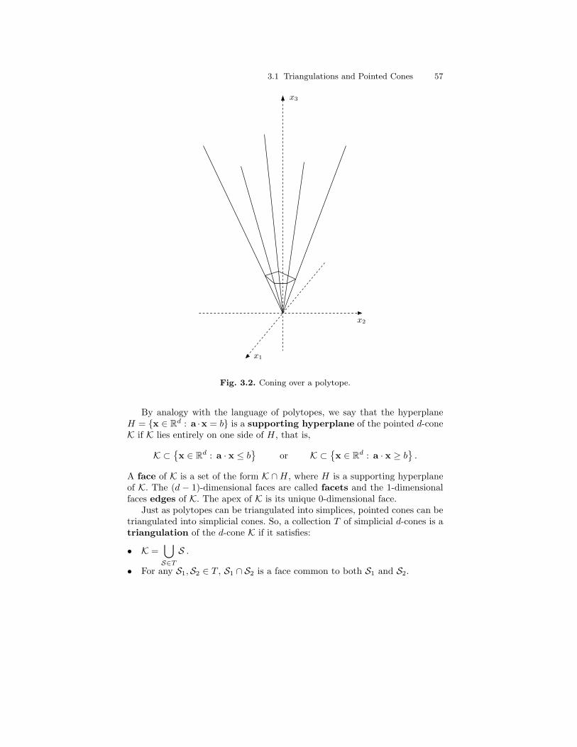
3.1 Triangulations and Pointed Cones 57
x3
x1
x2
Fig. 3.2. Coning over a polytope.
By analogy with the language of polytopes, we say that the hyperplaneH = {x ∈ Rd : a ·x = b} is a supporting hyperplane of the pointed d-coneK if K lies entirely on one side of H, that is,
K ⊂{x ∈ Rd : a · x ≤ b
}or K ⊂
{x ∈ Rd : a · x ≥ b
}.
A face of K is a set of the form K ∩H, where H is a supporting hyperplaneof K. The (d − 1)-dimensional faces are called facets and the 1-dimensionalfaces edges of K. The apex of K is its unique 0-dimensional face.
Just as polytopes can be triangulated into simplices, pointed cones can betriangulated into simplicial cones. So, a collection T of simplicial d-cones is atriangulation of the d-cone K if it satisfies:
• K =⋃S∈TS .
• For any S1,S2 ∈ T , S1 ∩ S2 is a face common to both S1 and S2.

58 3 Counting Lattice Points in Polytopes: The Ehrhart Theory
We say that K can be triangulated using no new generators if thereexists a triangulation T such that the generators of any S ∈ T are generatorsof P.
Theorem 3.2. Any pointed cone can be triangulated into simplicial cones us-ing no new generators.
Proof. This theorem is really a corollary to Theorem 3.1. Given a pointed d-cone K, there exists a hyperplane H that intersects K only at the apex. Nowtranslate H “into” the cone, so that H∩K consists of more than just one point.This intersection is a (d − 1)-polytope P, whose vertices are determined bythe generators of K. Now triangulate P using no new vertices. The cone overeach simplex of the triangulation is a simplicial cone. These simplicial cones,by construction, triangulate K. ut
3.2 Integer-Point Transforms for Rational Cones
We want to encode the information contained by the lattice points in a setS ⊂ Rd. It turns out that the following multivariate generating function allowsus to do this in an efficient way if S is a rational cone or polytope:
σS(z) = σS (z1, z2, . . . , zd) :=∑
m∈S∩Zdzm.
The generating function σS simply lists all integer points in S in a specialform: not as a list of vectors, but as a formal sum of monomials. We call σSthe integer-point transform of S; the function σS also goes by the namemoment generating function or simply generating function of S. The integer-point transform σS opens the door to both algebraic and analytic techniques.
Example 3.3. As a warm-up example, consider the 1-dimensional cone K =[0,∞). Its integer-point transform is our old friend
σK(z) =∑
m∈[0,∞)∩Z
zm =∑m≥0
zm =1
1− z. ut
Example 3.4. Now we consider the two-dimensional cone
K := {λ1(1, 1) + λ2(−2, 3) : λ1, λ2 ≥ 0} ⊂ R2
depicted in Figure 3.3. To obtain the integer-point transform σK, we tile Kby copies of the fundamental parallelogram
Π := {λ1(1, 1) + λ2(−2, 3) : 0 ≤ λ1, λ2 < 1} ⊂ R2.
More precisely, we translate Π by nonnegative integer linear combinationsof the generators (1, 1) and (−2, 3), and these translates will exactly cover

3.2 Integer-Point Transforms for Rational Cones 59
K. How can we list the integer points in K as monomials? Let’s first list allvertices of the translates of Π. These are nonnegative integer combinations ofthe generators (1, 1) and (−2, 3), so we can list them using geometric series:∑
m=j(1,1)+k(−2,3)j,k≥0
zm =∑j≥0
∑k≥0
zj(1,1)+k(−2,3) =1
(1− z1z2)(1− z−2
1 z32
) .We now use the integer points (m,n) ∈ Π to generate a subset of Z2 by addingto (m,n) nonnegative linear integer combinations of the generators (1, 1) and(−2, 3). Namely, we let
L(m,n) := {(m,n) + j(1, 1) + k(−2, 3) : j, k ∈ Z≥0} .
It is immediate that K∩Z2 is the disjoint union of the subsets L(m,n) as (m,n)ranges over Π ∩ Z2 = {(0, 0), (0, 1), (0, 2), (−1, 2), (−1, 3)}. Hence
σK(z) =(1 + z2 + z2
2 + z−11 z2
2 + z−11 z3
2
) ∑m=j(1,1)+k(−2,3)
j,k≥0
zm
=1 + z2 + z2
2 + z−11 z2
2 + z−11 z3
2
(1− z1z2)(1− z−2
1 z32
) . ut
x2
x1
(1, 1)
(−2, 3)
Fig. 3.3. The cone K and its fundamental parallelogram.
60 3 Counting Lattice Points in Polytopes: The Ehrhart Theory
Similar geometric series suffice to describe integer-point transforms forsimplicial d-cones. The following result utilizes the geometric series in severaldirections simultaneously.
Theorem 3.5. Suppose
K := {λ1w1 + λ2w2 + · · ·+ λdwd : λ1, λ2, . . . , λd ≥ 0}
is a simplicial d-cone, where w1,w2, . . . ,wd ∈ Zd. Then for v ∈ Rd, theinteger-point transform σv+K of the shifted cone v+K is the rational function
σv+K(z) =σv+Π(z)
(1− zw1) (1− zw2) · · · (1− zwd),
where Π is the half-open parallelepiped
Π := {λ1w1 + λ2w2 + · · ·+ λdwd : 0 ≤ λ1, λ2, . . . , λd < 1} .
The half-open parallelepiped Π is called the fundamental parallelepipedof K.
Proof. In σv+K(z) =∑
m∈(v+K)∩Zd zm, we list each integer point m in v +Kas the monomial zm. Such a lattice point can, by definition, be written as
m = v + λ1w1 + λ2w2 + · · ·+ λdwd
for some numbers λ1, λ2, . . . , λd ≥ 0. Because the wk’s form a basis of Rd, thisrepresentation is unique. Let’s write each of the λk’s in terms of their integerand fractional part: λk = bλkc+ {λk}. So
m = v+({λ1}w1+{λ2}w2+· · ·+{λd}wd
)+bλ1cw1+bλ2cw2+· · ·+bλdcwd ,
and we should note that, since 0 ≤ {λk} < 1, the vector
p := v + {λ1}w1 + {λ2}w2 + · · ·+ {λd}wd
is in v+Π. In fact, p ∈ Zd, since m and bλkcwk are all integer vectors. Againthe representation of p in terms of the wk’s is unique. In summary, we haveproved that any m ∈ v +K ∩ Zd can be uniquely written as
m = p + k1w1 + k2w2 + · · ·+ kdwd (3.1)
for some p ∈ (v + Π) ∩ Zd and some integers k1, k2, . . . , kd ≥ 0. On the otherhand, let us write the rational function on the right-hand side of the theoremas a product of series:
σv+Π(z)(1− zw1) · · · (1− zwd)
=
∑p∈(v+Π)∩Zd
zp
∑k1≥0
zk1w1
· · ·∑kd≥0
zkdwd
.
If we multiply everything out, a typical exponent will look exactly like (3.1).ut
3.2 Integer-Point Transforms for Rational Cones 61
Our proof contains a crucial geometric idea. Namely, we tile the cone v+Kwith translates of v + Π by nonnegative integral combinations of the wk’s. Itis this tiling that gives rise to the nice integer-point transform in Theorem 3.5.Computationally, we therefore favor cones over polytopes due to our abilityto tile a simplicial cone with copies of the fundamental domain, as above.Another reason for favoring cones over polytopes appears in Brion’s theoremin Chapter 9.
Theorem 3.5 shows that the real complexity of computing the integer-point transform σv+K is embedded in the location of the lattice points in theparallelepiped v + Π.
By mildly strengthening the hypothesis of Theorem 3.5, we obtain aslightly easier generating function, a result we shall need in Section 3.4 andChapter 4.
Corollary 3.6. Suppose
K := {λ1w1 + λ2w2 + · · ·+ λdwd : λ1, λ2, . . . , λd ≥ 0}
is a simplicial d-cone, where w1,w2, . . . ,wd ∈ Zd, and v ∈ Rd, such that theboundary of v +K contains no integer point. Then
σv+K(z) =σv+Π(z)
(1− zw1) (1− zw2) · · · (1− zwd),
where Π is the open parallelepiped
Π := {λ1w1 + λ2w2 + · · ·+ λdwd : 0 < λ1, λ2, . . . , λd < 1} .
Proof. The proof of Theorem 3.5 goes through almost verbatim, except thatv+Π now has no boundary lattice points, so that there is no harm in choosingΠ to be open. ut
Since a general pointed cone can always be triangulated into simplicialcones, the integer-point transforms add up in an inclusion–exclusion manner(note that the intersection of simplicial cones in a triangulation is again asimplicial cone, by Exercise 3.2). Hence we have the following corollary.
Corollary 3.7. Given any pointed cone
K = {v + λ1w1 + λ2w2 + · · ·+ λmwm : λ1, λ2, . . . , λm ≥ 0}
with v ∈ Rd, w1,w2, . . . ,wm ∈ Zd, the integer-point transform σK(z) evalu-ates to a rational function in the coordinates of z. ut
Philosophizing some more, one can show that the original infinite sumσK(z) converges only for z in a subset of Cd, whereas the rational functionthat represents σK gives us its meromorphic continuation. Later, in Chapters4 and 9, we make use of this continuation.

62 3 Counting Lattice Points in Polytopes: The Ehrhart Theory
3.3 Expanding and Counting Using Ehrhart’s OriginalApproach
Here is the fundamental theorem concerning the lattice-point count in anintegral convex polytope.
Theorem 3.8 (Ehrhart’s theorem). If P is an integral convex d-polytope,then LP(t) is a polynomial in t of degree d.
This result is due to Eugene Ehrhart, in whose honor we call LP theEhrhart polynomial of P. Naturally, there is an extension of Ehrhart’stheorem to rational polytopes, which we will discuss in Section 3.7.
Our proof of Ehrhart’s theorem uses generating functions of the form∑t≥0 f(t) zt, similar in spirit to the ones discussed in the beginning of Chap-
ter 1. If f is a polynomial, this power series takes on a special form, which weinvite the reader to prove (Exercise 3.8):
Lemma 3.9. If ∑t≥0
f(t) zt =g(z)
(1− z)d+1,
then f is a polynomial of degree d if and only if g is a polynomial of degree atmost d and g(1) 6= 0. ut
The reason we introduced generating functions of the form σS(z) =∑m∈S∩Zd zm in Section 3.2 is that they are extremely handy for lattice-point
problems. The connection to lattice points is evident, since we are summingover them. If we’re interested in the lattice-point count, we simply evaluateσS at z = (1, 1, . . . , 1):
σS(1, 1, . . . , 1) =∑
m∈S∩Zd1m =
∑m∈S∩Zd
1 = #(S ∩ Zd
).
(Here we denote by 1 a vector all of whose components are 1.) Naturally, weshould make this evaluation only if S is bounded; Theorem 3.5 already tellsus that it’s no fun evaluating σK(1) if K is a cone.
But the magic of the generating function σS does not stop there. To liter-ally take it to the next level, we cone over a convex polytope P. If P ⊂ Rd hasthe vertices v1,v2, . . . ,vn ∈ Zd, recall that we lift these vertices into Rd+1,by adding a 1 as their last coordinate. So let
w1 = (v1, 1) , w2 = (v2, 1) , . . . , wn = (vn, 1) .
Then
cone(P) = {λ1w1 + λ2w2 + · · ·+ λnwn : λ1, λ2, . . . , λn ≥ 0} ⊂ Rd+1.

3.3 Expanding and Counting Using Ehrhart’s Original Approach 63
Recall that we can recover our original polytope P by cutting cone(P) withthe hyperplane xd+1 = 1. We can recover more than just the original polytopein cone(P): By cutting the cone with the hyperplane xd+1 = 2, we obtain acopy of P dilated by a factor of 2. (The reader should meditate on why this cutis a 2-dilate of P.) More generally, we can cut the cone with the hyperplanexd+1 = t and obtain tP, as suggested by Figure 3.4.
Fig. 3.4. Recovering dilates of P in cone(P).
Now let’s form the integer-point transform σcone(P) of cone(P). By what wejust said, we should look at different powers of zd+1: there is one term (namely,1), with z0
d+1, corresponding to the origin; the terms with z1d+1 correspond to
lattice points in P (listed as monomials in z1, z2, . . . , zd), the terms with z2d+1
correspond to points in 2P, etc. In short,

64 3 Counting Lattice Points in Polytopes: The Ehrhart Theory
σcone(P) (z1, z2, . . . , zd+1)
= 1 + σP (z1, . . . , zd) zd+1 + σ2P (z1, . . . , zd) z2d+1 + · · ·
= 1 +∑t≥1
σtP (z1, . . . , zd) ztd+1 .
Specializing further for enumeration purposes, we recall that σP (1, 1, . . . , 1) =#(P ∩ Zd
), and so
σcone(P) (1, 1, . . . , 1, zd+1) = 1 +∑t≥1
σtP (1, 1, . . . , 1) ztd+1
= 1 +∑t≥1
#(tP ∩ Zd
)ztd+1 .
But by definition, the enumerators on the right-hand side are just evaluationsof Ehrhart’s counting function, that is, σcone(P) (1, 1, . . . , 1, zd+1) is nothingbut the Ehrhart series of P:
Lemma 3.10. σcone(P) (1, 1, . . . , 1, z) = 1 +∑t≥1
LP(t) zt = EhrP(z) . ut
With all this machinery at hand, we can prove Ehrhart’s theorem.
Proof of Theorem 3.8. It suffices to prove the theorem for simplices, becausewe can triangulate any integral polytope into integral simplices, using no newvertices. Note that these simplices will intersect in lower-dimensional integralsimplices.
By Lemma 3.9, it suffices to prove that for an integral d-simplex ∆,
Ehr∆(z) = 1 +∑t≥1
L∆(t) zt =g(z)
(1− z)d+1
for some polynomial g of degree at most d with g(1) 6= 0. In Lemma 3.10we showed that the Ehrhart series of ∆ equals σcone(∆) (1, 1, . . . , 1, z), so let’sstudy the integer-point transform attached to cone(∆).
The simplex ∆ has d+ 1 vertices v1,v2, . . . ,vd+1, and so cone(∆) ⊂ Rd+1
is simplicial, with apex the origin and generators
w1 = (v1, 1) , w2 = (v2, 1) , . . . , wd+1 = (vd+1, 1) ∈ Zd+1.
Now we use Theorem 3.5:
σcone(∆) (z1, z2, . . . , zd+1) =σΠ (z1, z2, . . . , zd+1)
(1− zw1) (1− zw2) · · · (1− zwd+1),
where Π = {λ1w1 + λ2w2 + · · ·+ λd+1wd+1 : 0 ≤ λ1, λ2, . . . , λd+1 < 1}. Thisparallelepiped is bounded, so the attached generating function σΠ is a Laurentpolynomial in z1, z2, . . . , zd+1.

3.4 The Ehrhart Series of an Integral Polytope 65
We claim that the zd+1-degree of σΠ is at most d. In fact, since the xd+1-coordinate of each wk is 1, the xd+1-coordinate of a point in Π is λ1+λ2+· · ·+λd+1 for some 0 ≤ λ1, λ2, . . . , λd+1 < 1. But then λ1 +λ2 + · · ·+λd+1 < d+1,so if this sum is an integer it is at most d, which implies that the zd+1-degreeof σΠ (z1, z2, . . . , zd+1) is at most d. Consequently, σΠ (1, 1, . . . , 1, zd+1) is apolynomial in zd+1 of degree at most d. The evaluation σΠ (1, 1, 1, . . . , 1) of thispolynomial at zd+1 = 1 is not zero, because σΠ (1, 1, 1, . . . , 1) = #
(Π ∩ Zd+1
)and the origin is a lattice point in Π.
Finally, if we specialize zwk to z1 = z2 = · · · = zd = 1, we obtain z1d+1, so
that
σcone(∆) (1, 1, . . . , 1, zd+1) =σΠ (1, 1, . . . , 1, zd+1)
(1− zd+1)d+1.
The left–hand side is Ehr∆ (zd+1) = 1 +∑t≥1 L∆(t) ztd+1 by Lemma 3.10. ut
3.4 The Ehrhart Series of an Integral Polytope
We can actually take our proof of Ehrhart’s theorem one step further by study-ing the polynomial σΠ (1, 1, . . . , 1, zd+1). As mentioned above, the coefficientof zkd+1 simply counts the integer points in the parallelepiped Π cut with thehyperplane xd+1 = k. Let us record this.
Corollary 3.11. Suppose ∆ is an integral d-simplex with vertices v1,v2, . . . ,vd+1, and let wj = (vj , 1). Then
Ehr∆(z) = 1 +∑t≥1
L∆(t) zt =hd z
d + hd−1 zd−1 + · · ·+ h1 z + h0
(1− z)d+1,
where hk equals the number of integer points in
{λ1w1 + λ2w2 + · · ·+ λd+1wd+1 : 0 ≤ λ1, λ2, . . . , λd+1 < 1}
with last variable equal to k. ut
This result can actually be used to compute Ehr∆, and therefore theEhrhart polynomial, of an integral simplex ∆ in low dimensions very quickly(a fact that the reader may discover in some of the exercises). We remark,however, that things are not as simple for arbitrary integral polytopes. Notonly is triangulation a nontrivial task in general, but one would also have todeal with overcounting where simplices of a triangulation meet.
Corollary 3.11 implies that the numerator of the Ehrhart series of an inte-gral simplex has nonnegative coefficients, since those coefficients count some-thing. Although the latter cannot be said of the coefficients of the Ehrhartseries of a general integral polytope, the nonnegativity property magicallysurvives.
66 3 Counting Lattice Points in Polytopes: The Ehrhart Theory
Theorem 3.12 (Stanley’s nonnegativity theorem). Suppose P is an in-tegral convex d-polytope with Ehrhart series
EhrP(z) =hd z
d + hd−1 zd−1 + · · ·+ h0
(1− z)d+1.
Then h0, h1, . . . , hd are nonnegative integers.
Proof. Triangulate cone(P) ⊂ Rd+1 into the simplicial cones K1,K2, . . . ,Km.Now Exercise 3.14 ensures that there exists a vector v ∈ Rd+1 such that
cone(P) ∩ Zd+1 = (v + cone(P)) ∩ Zd+1
(that is, we neither lose nor gain any lattice points when shifting cone(P) byv) and neither the facets of v + cone(P) nor the triangulation hyperplanescontain any lattice points. This implies that every lattice point in v+cone(P)belongs to exactly one simplicial cone v +Kj :
cone(P) ∩ Zd+1 = (v + cone(P)) ∩ Zd+1 =m⋃j=1
((v +Kj) ∩ Zd+1
), (3.2)
and this union is a disjoint union. If we translate the last identity intogenerating-function language, it becomes
σcone(P) (z1, z2, . . . , zd+1) =m∑j=1
σv+Kj (z1, z2, . . . , zd+1) .
But now we recall that the Ehrhart series of P is just a special evaluation ofσcone(P) (Lemma 3.10):
EhrP(z) = σcone(P) (1, 1, . . . , 1, z) =m∑j=1
σv+Kj (1, 1, . . . , 1, z) . (3.3)
It suffices to show that the rational generating functions σv+Kj (1, 1, . . . , 1, z)for the simplicial cones v + Kj have nonnegative integer numerator. Butthis fact follows from evaluating the rational function in Corollary 3.6 at(1, 1, . . . , 1, z). ut
This proof shows a little more: Since the origin is in precisely one simplicialcone on the right-hand side of (3.2), we get on the right-hand side of (3.3)precisely one term that contributes 1/(1 − z)d+1 to EhrP ; all other termscontribute to higher powers of the numerator polynomial of EhrP . That is,the constant term h0 equals 1. The reader might feel that we are chasing ourtail at this point, since we assumed from the very beginning that the constantterm of the infinite series EhrP is 1, and hence h0 has to be 1, as a quick lookat the expansion of the rational function representing EhrP shows. The aboveargument shows merely that this convention is geometrically sound. Let usrecord this:
3.4 The Ehrhart Series of an Integral Polytope 67
Lemma 3.13. Suppose P is an integral convex d-polytope with Ehrhart series
EhrP(z) =hd z
d + hd−1 zd−1 + · · ·+ h0
(1− z)d+1.
Then h0 = 1. ut
For a general integral polytope P, the reader has probably already discov-ered how to extract the Ehrhart polynomial of P from its Ehrhart series:
Lemma 3.14. Suppose P is an integral convex d-polytope with Ehrhart series
EhrP(z) = 1 +∑t≥1
LP(t) zt =hd z
d + hd−1 zd−1 + · · ·+ h1 z + 1
(1− z)d+1.
Then
LP(t) =(t+ d
d
)+ h1
(t+ d− 1
d
)+ · · ·+ hd−1
(t+ 1d
)+ hd
(t
d
).
Proof. Expand into a binomial series:
EhrP(z) =hd z
d + hd−1 zd−1 + · · ·+ h1 z + 1
(1− z)d+1
=(hd z
d + hd−1 zd−1 + · · ·+ h1 z + 1
)∑t≥0
(t+ d
d
)zt
= hd∑t≥0
(t+ d
d
)zt+d + hd−1
∑t≥0
(t+ d
d
)zt+d−1 + · · ·
+ h1
∑t≥0
(t+ d
d
)zt+1 +
∑t≥0
(t+ d
d
)zt
= hd∑t≥d
(t
d
)zt + hd−1
∑t≥d−1
(t+ 1d
)zt + · · ·
+ h1
∑t≥1
(t+ d− 1
d
)zt +
∑t≥0
(t+ d
d
)zt.
In all infinite sums on the right-hand side, we can start the index t with 0without changing the sums, by the definition (2.1) of the binomial coefficient.Hence
EhrP(z)
=∑t≥0
(hd
(t
d
)+ hd−1
(t+ 1d
)+ · · ·+ h1
(t+ d− 1
d
)+(t+ d
d
))zt.
ut
68 3 Counting Lattice Points in Polytopes: The Ehrhart Theory
The representation of the polynomial LP(t) in terms of the coefficientsof EhrP can be interpreted as the Ehrhart polynomial expressed in the basis(td
),(t+1d
), . . . ,
(t+dd
)(see Exercise 3.9). This representation is very useful, as
the following results show.
Corollary 3.15. If P is an integral convex d-polytope, then the constant termof the Ehrhart polynomial LP is 1.
Proof. Use the expansion of Lemma 3.14. The constant term is
LP(0) =(d
d
)+ h1
(d− 1d
)+ · · ·+ hd−1
(1d
)+ hd
(0d
)=(d
d
)= 1 . ut
This proof is exciting, because it marks the first instance where we extendthe domain of an Ehrhart polynomial beyond the positive integers, for whichthe lattice-point enumerator was initially defined. More precisely, Ehrhart’stheorem (Theorem 3.8) implies that the counting function
LP(t) = #(tP ∩ Zd
),
originally defined for positive integers t, can be extended to all real or evencomplex arguments t (as a polynomial). A natural question arises: are therenice interpretations of LP(t) for arguments t that are not positive integers?Corollary 3.15 gives such an interpretation for t = 0. In Chapter 4, we willgive interpretations of LP(t) for negative integers t.
Corollary 3.16. Suppose P is an integral convex d-polytope with Ehrhart se-ries
EhrP(z) =hd z
d + hd−1 zd−1 + · · ·+ h1 z + 1
(1− z)d+1.
Then h1 = LP(1)− d− 1 = #(P ∩ Zd
)− d− 1.
Proof. Use the expansion of Lemma 3.14 with t = 1:
LP(1) =(d+ 1d
)+ h1
(d
d
)+ · · ·+ hd−1
(2d
)+ hd
(1d
)= d+ 1 + h1 . ut
The proof of Corollary 3.16 suggests that there are also formulas forh2, h3, . . . in terms of the evaluations LP(1), LP(2), . . . , and we invite thereader to find them (Exercise 3.10).
A final corollary to Theorem 3.12 and Lemma 3.14 states how large thedenominators of the Ehrhart coefficients can be:
Corollary 3.17. Suppose P is an integral polytope with Ehrhart polynomialLP(t) = cd t
d+cd−1 td−1 + · · ·+c1 t+1. Then all coefficients satisfy d! ck ∈ Z.
3.5 From the Discrete to the Continuous Volume of a Polytope 69
Proof. By Theorem 3.12 and Lemma 3.14,
LP(t) =(t+ d
d
)+ h1
(t+ d− 1
d
)+ · · ·+ hd−1
(t+ 1d
)+ hd
(t
d
),
where the hk’s are integers. Hence multiplying out this expression yields apolynomial in t whose coefficients can be written as rational numbers withdenominator d!. ut
We finish this section with a general result that gives relations betweennegative integer roots of a polynomial and its generating function. This the-orem will become handy in Chapter 4, in which we find an interpretation forthe evaluation of an Ehrhart polynomial at negative integers.
Theorem 3.18. Suppose p is a degree-d polynomial with the rational gener-ating function∑
t≥0
p(t) zt =hd z
d + hd−1 zd−1 + · · ·+ h1 z + h0
(1− z)d+1.
Then hd = hd−1 = · · · = hk+1 = 0 and hk 6= 0 if and only if p(−1) = p(−2) =· · · = p (−(d− k)) = 0 and p (−(d− k + 1)) 6= 0.
Proof. Suppose hd = hd−1 = · · · = hk+1 = 0 and hk 6= 0. Then the proof ofLemma 3.14 gives
p(t) = h0
(t+ d
d
)+ · · ·+ hk−1
(t+ d− k + 1
d
)+ hk
(t+ d− k
d
).
All the binomial coefficients are zero for t = −1,−2, . . . ,−d+ k, so those areroots of p. On the other hand, all binomial coefficients but the last one arezero for t = −d+ k − 1, and since hk 6= 0, −d+ k − 1 is not a root of p.
Conversely, suppose p(−1) = p(−2) = · · · = p (−(d− k)) = 0 andp (−(d− k + 1)) 6= 0. The first root −1 of p gives
0 = p(−1) = h0
(d− 1d
)+h1
(d− 2d
)+ · · ·+hd−1
(0d
)+hd
(−1d
)= hd
(−1d
),
so we must have hd = 0. The next root −2 forces hd−1 = 0, and so on, up tothe root −d+ k, which forces hk+1 = 0. It remains to show that hk 6= 0. Butif hk were zero then, by a similar line of reasoning as in the first part of theproof, p(−d+ k − 1) = 0, a contradiction. ut
3.5 From the Discrete to the Continuous Volume of aPolytope
Given a geometric object S ⊂ Rd, its volume, defined by the integral volS :=∫Sdx, is one of the fundamental data of S. By the definition of the integral, say
70 3 Counting Lattice Points in Polytopes: The Ehrhart Theory
in the Riemannian sense, we can think of computing volS by approximatingS with d-dimensional boxes that get smaller and smaller. To be precise, ifwe take the boxes with side length 1/t then they each have volume 1/td. Wemight further think of the boxes as filling out the space between grid points inthe lattice
(1tZ)d. This means that volume computation can be approximated
by counting boxes, or equivalently, lattice points in(
1tZ)d:
volS = limt→∞
1td·#
(S ∩
(1tZ)d)
.
It is a short step to counting integer points in dilates of S, because
#
(S ∩
(1tZ)d)
= #(tS ∩ Zd
).
Let us summarize:
Lemma 3.19. Suppose S ⊂ Rd is d-dimensional. Then
volS = limt→∞
1td·#(tS ∩ Zd
). ut
We emphasize here that S is d-dimensional, because otherwise (since S couldbe lower-dimensional although living in d-space), by our current definitionvolS = 0. (We will extend our volume definition in Chapter 5 to give nonzerorelative volume to objects that are not full-dimensional.)
Part of the magic of Ehrhart’s theorem lies in the fact that for an integrald-polytope P, we do not have to take a limit to compute volP; we need tocompute “only” the d+ 1 coefficients of a polynomial.
Corollary 3.20. Suppose P ⊂ Rd is an integral convex d-polytope withEhrhart polynomial cd td + cd−1 t
d−1 + · · ·+ c1 t+ 1. Then cd = volP.
Proof. By Lemma 3.19,
volP = limt→∞
cd td + cd−1 t
d−1 + · · ·+ c1 t+ 1td
= cd . ut
On the one hand, this should not come as a surprise, because countinginteger points in some object should grow roughly like the volume of theobject as we make it bigger and bigger. On the other hand, the fact that wecan compute the volume as one term of a polynomial should be very surprising:the polynomial is a counting function and as such is something discrete, yet bycomputing it (and its leading term), we derive some continuous data. Evenmore, we can—at least theoretically—compute this continuous datum (thevolume) of the object by calculating a few values of the polynomial and theninterpolating; this can be described as a completely discrete operation!
We finish this section by showing how to retrieve the continuous volumeof an integer polytope from its Ehrhart series.
3.6 Interpolation 71
Corollary 3.21. Suppose P ⊂ Rd is an integral convex d-polytope, and
EhrP(z) =hd z
d + hd−1 zd−1 + · · ·+ h1 z + 1
(1− z)d+1.
Then volP =1d!
(hd + hd−1 + · · ·+ h1 + 1) .
Proof. Use the expansion of Lemma 3.14. The leading coefficient is
1d!
(hd + hd−1 + · · ·+ h1 + 1) . ut
3.6 Interpolation
We now use the polynomial behavior of the discrete volume LP of an integralpolytope P to compute the continuous volume volP and the discrete volumeLP from finite data.
Two points uniquely determine a line. There exists a unique quadraticpassing through any three given points. In general, a degree-d polynomialp is determined by d + 1 points (x, p(x)) ∈ R2. Namely, evaluating p(x) =cdx
d + cd−1xd−1 + · · ·+ c0 at distinct inputs x1, x2, . . . , xd+1 gives
p (x1)p (x2)
...p (xd+1)
= V
cdcd−1
...c0
, (3.4)
where
V =
xd1 xd−1
1 · · · x1 1xd2 xd−1
2 · · · x2 1...
......
...xdd+1 x
d−1d+1 · · · xd+1 1
,
so that cdcd−1
...c0
= V−1
p (x1)p (x2)
...p (xd+1)
. (3.5)
(Exercise 3.16 makes sure that V is invertible.) The identity (3.5) gives thefamous Lagrange interpolation formula.
This gives us an efficient way to compute LP , at least when dimP is nottoo large. The continuous volume of P will follow instantly, since it is theleading coefficient cd of LP . In the case of an Ehrhart polynomial LP , weknow that LP(0) = 1, so that (3.4) simplifies to

72 3 Counting Lattice Points in Polytopes: The Ehrhart TheoryLP (x1)− 1LP (x2)− 1
...LP (xd)− 1
=
xd1 x
d−11 · · · x1
xd2 xd−12 · · · x2
......
...xdd x
d−1d · · · xd
cdcd−1
...c1
.
Example 3.22 (Reeve’s tetrahedron). Let Th be the tetrahedron withvertices (0, 0, 0), (1, 0, 0), (0, 1, 0), and (1, 1, h), where h is a positive integer(see Figure 3.5).
2h
h
(2, 2, 2h)
(1, 1, h)
1
2
1 2
x
y
z
Fig. 3.5. Reeve’s tetrahedron Th (and 2Th).
To interpolate the Ehrhart polynomial LTh(t) from its values at variouspoints, we use Figure 3.5 to deduce the following:
4 = LTh(1) = vol (Th) + c2 + c1 + 1 ,
h+ 9 = LTh(2) = vol (Th) · 23 + c2 · 22 + c1 · 2 + 1 .
Using the volume formula for a pyramid, we know that

3.7 Rational Polytopes and Ehrhart Quasipolynomials 73
vol (Th) =13
(base area)(height) =h
6.
Thus h+ 1 = h+ 2c2 − 1, which gives us c2 = 1 and c1 = 2− h6 . Therefore
LTh(t) =h
6t3 + t2 +
(2− h
6
)t+ 1 . ut
3.7 Rational Polytopes and Ehrhart Quasipolynomials
We do not have to change much to study lattice-point enumeration for rationalpolytopes, and most of this section will consist of exercises for the reader. Thestructural result paralleling Theorem 3.8 is as follows.
Theorem 3.23 (Ehrhart’s theorem for rational polytopes). If P is arational convex d-polytope, then LP(t) is a quasipolynomial in t of degreed. Its period divides the least common multiple of the denominators of thecoordinates of the vertices of P.
We will call the least common multiple of the denominators of the co-ordinates of the vertices of P the denominator of P. Theorem 3.23, alsodue to Ehrhart, extends Theorem 3.8, because the denominator of an integralpolytope P is one. Exercises 3.21 and 3.22 show that the word “divides” inTheorem 3.23 is far from being replaceable by “equals.”
We start the path toward a proof of Theorem 3.23 by stating the analogueof Lemma 3.9 for quasipolynomials (see Exercise 3.19):
Lemma 3.24. If ∑t≥0
f(t) zt =g(z)h(z)
,
then f is a quasipolynomial of degree d with period dividing p if and only if gand h are polynomials such that deg(g) < deg(h), all roots of h are pth rootsof unity of multiplicity at most d+ 1, and there is a root of multiplicity equalto d+1 (all of this assuming that g/h has been reduced to lowest terms). ut
Our goal is now evident: we will prove that if P is a rational convex d-polytope with denominator p, then
EhrP(z) = 1 +∑t≥1
LP(t) zt =g(z)
(1− zp)d+1,
for some polynomial g of degree less than p(d+ 1). As in Section 3.3, we willhave to prove this only for the case of a rational simplex. So suppose the d-simplex ∆ has vertices v1,v2, . . . ,vd+1 ∈ Qd, and the denominator of ∆ is p.Again we will cone over ∆: let
74 3 Counting Lattice Points in Polytopes: The Ehrhart Theory
w1 = (v1, 1) ,w2 = (v2, 1) , . . . ,wd+1 = (vd+1, 1) ;
then
cone(∆) = {λ1w1 + λ2w2 + · · ·+ λd+1wd+1 : λ1, λ2, . . . , λd+1 ≥ 0} ⊂ Rd+1.
To be able to use Theorem 3.5, we first have to ensure that we have a descrip-tion of cone(∆) with integral generators. But since the denominator of ∆ is p,we can replace each generator wk by pwk ∈ Zd+1, and we’re ready to applyTheorem 3.5. From this point, the proof of Theorem 3.23 proceeds exactly likethat of Theorem 3.8, and we invite the reader to finish it up (Exercise 3.20).
Although the proofs of Theorem 3.23 and Theorem 3.8 are almost identical,the arithmetic structure of Ehrhart quasipolynomials is much more subtle andless well known than that of Ehrhart polynomials.
3.8 Reflections on the Coin-Exchange Problem and theGallery of Chapter 2
At this point, we encourage the reader to look back at the first two chapters inlight of the basic Ehrhart-theory results. Popoviciu’s theorem (Theorem 1.5)and its higher-dimensional analogue give a special set of Ehrhart quasipoly-nomials. On the other hand, in Chapter 2 we encountered many integral poly-topes. Ehrhart’s theorem (Theorem 3.8) explains why their lattice-point enu-meration functions were all polynomials.
Notes
1. Triangulations of polytopes and manifolds are an active source of researchwith many interesting open problems; see, e.g., [69].
2. Eugene Ehrhart laid the foundation for the central theme of this book inthe 1960s, starting with the proof of Theorem 3.8 in 1962 [79]. The proof wegive here follows Ehrhart’s original lines of thought. An interesting fact is thathe did his most beautiful work as a teacher at a lycee in Strasbourg (France),receiving his doctorate at age 60 on the urging of some colleagues.
3. Given any d linearly independent vectors w1,w2, . . . ,wd ∈ Rd, the lat-tice generated by them is the set of all integer linear combinations ofw1,w2, . . . ,wd. Alternatively, one can define a lattice as a discrete subgroupof Rd, and these two notions can be shown to be equivalent. One might won-der whether replacing the lattice Zd by an arbitrary lattice L throughout thestatements of the theorems—requiring now that the vertices of a polytope bein L—gives us any different results. The fact that the theorems of this chapter

Exercises 75
remain the same follows from the observation that any lattice can be mappedto Zd by an invertible linear transformation.
4. Richard Stanley developed much of the theory of Ehrhart (quasi-)polyno-mials, initially from a commutative-algebra point of view. Theorem 3.12 isdue to him [170]. The proof we give here appeared in [30]. An extension ofTheorem 3.12 was found by Takayuki Hibi; he proved that if hd > 0 thenhk ≥ h1 for all 1 ≤ k ≤ d− 1 (using the notation of Theorem 3.12) [98].
5. The tetrahedron Th of Example 3.22 was used by John Reeve to show thatPick’s theorem does not hold in R3 (see Exercise 3.18) [154]. Incidentally, theformula for LTh also proves that the coefficients of an Ehrhart polynomial (ofa closed polytope) are not always positive.
6. There are several interesting questions (some of which are still open) regard-ing the periods of Ehrhart quasipolynomials. Some particularly nice examplesabout what can happen with periods were given by Tyrrell McAllister andKevin Woods [126].
7. Most of the results remain true if we replace “convex polytope” by “poly-topal complex,” that is, a finite union of polytopes. One important exceptionis Corollary 3.15: the constant term of an “Ehrhart polynomial” of an integralpolytopal complex C is the Euler characteristic of C.
8. The reader might wonder why we do not discuss polytopes with irrationalvertices. The answer is simple: nobody has yet found a theory that would par-allel the results in this chapter, even in dimension two. One notable exceptionis [11], in which irrational extensions of Brion’s theorem are given; we willstudy the rational case of Brion’s theorem in Chapter 9. On the other hand,Ehrhart theory has been extended to functions other than strict lattice-pointcounting; one instance is described in Chapter 11.
Exercises
3.1. To any permutation π ∈ Sd on d elements, we associate the simplex
∆π := conv{0, eπ(1), eπ(1) + eπ(2), . . . , eπ(1) + eπ(2) + · · ·+ eπ(d)
},
where e1, e2, . . . , ed denote the unit vectors in Rd.
(a) Prove that {∆π : π ∈ Sd} is a triangulation of the unit d-cube [0, 1]d.(b) Prove that all ∆π are congruent to each other, that is, each one can be
obtained from any other by reflections, translations, and rotations.(c) Show that for all π ∈ Sd, L∆π
(t) =(d+td
).
76 3 Counting Lattice Points in Polytopes: The Ehrhart Theory
3.2. ♣ Suppose T is a triangulation of a pointed cone. Prove that the inter-section of two simplicial cones in T is again a simplicial cone.
3.3. Find the generating function σK(z) for the following cones:
(a) K = {λ1(0, 1) + λ2(1, 0) : λ1, λ2 ≥ 0} ;(b) K = {λ1(0, 1) + λ2(1, 1) : λ1, λ2 ≥ 0} ;(c) K = {(3, 4) + λ1(0, 1) + λ2(2, 1) : λ1, λ2 ≥ 0} .
3.4. ♣ Let S ⊆ Rm and T ⊆ Rn. Show that σS×T (z1, z2, . . . , zm+n) =σS (z1, z2, . . . , zm)σT (zm+1, zm+2, . . . , zm+n) .
3.5. ♣ Let K be a rational d-cone, and let m ∈ Zd. Show that σm+K(z) =zmσK(z).
3.6. ♣ For a set S ⊂ Rd, let −S := {−x : x ∈ S}. Prove that
σ−S (z1, z2, . . . , zd) = σS
(1z1,
1z2, . . . ,
1zd
).
3.7. Given a pointed cone K ⊂ Rd with apex at the origin, let S := K ∩ Zd.Show that if x,y ∈ S then x + y ∈ S. (In algebraic terms, S is a semi-group, since 0 ∈ S and associativity of the addition in S follows trivially fromassociativity in Rd.)
3.8. ♣ Prove Lemma 3.9: If∑t≥0
f(t) zt =g(z)
(1− z)d+1,
then f is a polynomial of degree d if and only if g is a polynomial of degreeat most d and g(1) 6= 0.
3.9. Prove that(x+nn
),(x+n−1n
), . . . ,
(xn
)is a basis for the vector space Poln of
polynomials (in the variable x) of degree less than or equal to n.
3.10. For a polynomial p(t) = cdtd + cd−1t
d−1 + · · ·+ c0, let Hp(z) be definedby ∑
t≥0
p(t) zt =Hp(z)
(1− z)d+1.
Consider the map φd : Pold → Pold, p 7→ Hp.
(a) Show that φd is a linear transformation.(b) Compute the matrix describing φd for d = 0, 1, 2, . . . .(c) Deduce formulas for h2, h3, . . . , similar to the one in Corollary 3.16.
3.11. Compute the Ehrhart polynomials and the Ehrhart series of the sim-plices with the following vertices:

Exercises 77
(a) (0, 0, 0), (1, 0, 0), (0, 2, 0), and (0, 0, 3);(b) (0, 0, 0, 0), (1, 0, 0, 0), (0, 2, 0, 0), (0, 0, 3, 0), and (0, 0, 0, 4).
3.12. Define the hypersimplex ∆(d, k) as the convex hull of
{ej1 + ej2 + · · ·+ ejk : 1 ≤ j1 < j2 < · · · < jk ≤ d} ,
where e1, e2, . . . , ed are the standard basis vectors in Rd. For example, ∆(d, 1)and ∆(d, d−1) are regular (d−1)-simplices. Compute the Ehrhart polynomialand the Ehrhart series of ∆(d, k).
3.13. ♣ Suppose H is the hyperplane given by
H ={x ∈ Rd : a1x1 + a2x2 + · · ·+ adxd = 0
}for some a1, a2, . . . , ad ∈ Z, which we may assume to have no common factor.Prove that there exists v ∈ Zd such that
⋃n∈Z
((nv +H) ∩ Zd
)= Zd. (This
implies, in particular, that the points in Zd \H are all at least some minimaldistance away from H; this minimal distance is essentially given by the dotproduct of v with (a1, a2, . . . , ad).)
3.14. ♣ A hyperplane H is rational if it can be written in the form
H ={x ∈ Rd : a1x1 + a2x2 + · · ·+ adxd = b
}for some a1, a2, . . . , ad, b ∈ Z. A hyperplane arrangement in Rd is a finiteset of hyperplanes in Rd. Prove that a rational hyperplane arrangement Hcan be translated so that no hyperplane in H contains any integer points.
3.15. The conclusion of the previous exercise can be strengthened: Prove thata rational hyperplane arrangement H can be translated such that no hyper-plane in H contains any rational points.
3.16. Show that, given distinct numbers x1, x2, . . . , xd+1, the matrix
V =
xd1 xd−1
1 · · · x1 1xd2 xd−1
2 · · · x2 1...
......
...xdd+1 x
d−1d+1 · · · xd+1 1
is not singular. (V is known as the Vandermonde matrix.)
3.17. Let P be an integral d-polytope. Show that
volP =1d!
((−1)d +
d∑k=1
(d
k
)(−1)d−kLP(k)
).

78 3 Counting Lattice Points in Polytopes: The Ehrhart Theory
3.18. As in Example 3.22, let Tn be the tetrahedron with vertices (0, 0, 0),(1, 0, 0), (0, 1, 0), and (1, 1, n), where n is a positive integer. Show that thevolume of Tn is unbounded as n → ∞, yet for all n, Tn has no interior andfour boundary lattice points. This example proves that Pick’s theorem doesnot hold for a three-dimensional integral polytope P, in the sense that thereis no linear relationship among volP, LP(1), and LP◦(1).
3.19. ♣ Prove Lemma 3.24: If∑t≥0
f(t) zt =g(z)h(z)
,
then f is a quasipolynomial of degree d with period dividing p if and only if gand h are polynomials such that deg(g) < deg(h), all roots of h are pth rootsof unity of multiplicity at most d+ 1, and there is a root of multiplicity equalto d+ 1 (all of this assuming that g/h has been reduced to lowest terms).
3.20. ♣ Provide the details for the proof of Theorem 3.23: If P is a rationalconvex d-polytope, then LP(t) is a quasipolynomial in t of degree d. Its perioddivides the least common multiple of the coordinates of the vertices of P.
3.21. Let T be the rational triangle with vertices (0, 0),(
1, p−1p
), and (p, 0),
where p is a fixed integer ≥ 2. Show that LT (t) = p−12 t2 + p+1
2 t + 1; inparticular, LT is a polynomial.
3.22. Prove that for any d ≥ 2 and any p ≥ 1, there exists a d-polytope Pwhose Ehrhart quasipolynomial is a polynomial (i.e., it has period 1), yet Phas a vertex with denominator p.
3.23. Prove that the period of the Ehrhart quasipolynomial of a 1-dimensionalpolytope is always equal to the lcm of the denominators of its vertices.
3.24. Let T be the triangle with vertices(− 1
2 ,−12
),(
12 ,−
12
), and
(0, 3
2
). Show
that LT (t) = t2 + c(t) t+ 1, where
c(t) =
{1 if t is even,0 if t is odd.
(This shows that the periods of the “coefficients” of an Ehrhart quasipoly-nomial do not necessarily increase with decreasing power.) Find the Ehrhartseries of T .
3.25. Prove the following extension of Theorem 3.12: Suppose P is a rationald-polytope with denominator p. Then
EhrP(z) =f(z)
(1− zp)d+1,
where f is a polynomial with nonnegative integral coefficients.

Exercises 79
3.26. Find and prove a statement that extends Lemma 3.14 to Ehrhartquasipolynomials.
3.27. Prove the following extension of Corollary 3.15 to rational polytopes.Namely, the Ehrhart quasipolynomial LP of the rational convex polytopeP ⊂ Rd satisfies LP(0) = 1.
3.28. Prove the following analogue of Corollary 3.17 for rational polytopes:Suppose P is a rational polytope with Ehrhart quasipolynomial LP(t) =cd(t) td + cd−1(t) td−1 + · · ·+ c1(t) t+ c0(t). Then for all t ∈ Z and 0 ≤ k ≤ d,we have d! ck(t) ∈ Z.
3.29. ♣ Prove that Corollary 3.20 also holds for rational polytopes: Sup-pose P ⊂ Rd is a rational convex d-polytope with Ehrhart quasipolynomialcd(t) td + cd−1(t) td−1 + · · · + c0(t). Then cd(t) equals the volume of P; inparticular, cd(t) is constant.
3.30. Suppose P is a rational convex polytope. Show that as rational func-tions,
Ehr2P(z) =12(EhrP
(√z)
+ EhrP(−√z)).
3.31. Suppose f and g are quasipolynomials. Prove that the convolution
F (t) :=t∑
s=0
f(s) g(t− s)
is also a quasipolynomial. What can you say about the degree and the periodof F , given the degrees and periods of f and g?
3.32. Given two positive, relatively prime integers a and b, let
f(t) :=
{1 if a|t,0 otherwise,
and g(t) :=
{1 if b|t,0 otherwise.
Form the convolution of f and g. What function is it?
3.33. Suppose P ⊂ Rm and Q ⊂ Rn are rational polytopes. Prove that theconvolution of LP and LQ equals the Ehrhart quasipolynomial of the polytopegiven by the convex hull of P × {0n} × {0} and {0m} × Q × {1}. Here 0ddenotes the origin in Rd.
3.34. We define the unimodular group SLd (Z) as the set of all d×dmatriceswith integer entries and determinant ±1.
(a) Show that SLd (Z) acts on the integer lattice Zd as a one-to-one, ontomap. That is, fix any A ∈ SLd (Z). Then A maps Zd to itself in a bijectivefashion.

80 3 Counting Lattice Points in Polytopes: The Ehrhart Theory
(b) For any open simplex ∆◦ ⊂ Rd and any A ∈ SLd (Z), consider the imageof ∆◦ under A, defined by A (∆◦) := {A x : x ∈ ∆◦}. Show that
#{
∆◦ ∩ Zd}
= #{A (∆◦) ∩ Zd
}.
(c) Let P be an integral polytope, and let Q := A (P), where A ∈ SLd (Z),so that P and Q are unimodular images of each other. Show that LP(t) =LQ(t). (Hint: Write P as the disjoint union of open simplices.)
3.35. Search on the Internet for the program LattE: Lattice-Point Enumera-tion [66, 115]. You can download it for free. Experiment.
Open Problems
3.36. How many triangulations are there for a given polytope?
3.37. What is the minimal number of simplices needed to triangulate the unitd-cube? (These numbers are known for d ≤ 7.)
3.38. Classify the polynomials of a fixed degree d that are Ehrhart polyno-mials. This is completely done for d = 2 [160] and partially known for d = 3and 4 [24, Section 3].
3.39. Study the roots of Ehrhart polynomials of integral polytopes in a fixeddimension [24, 37, 42, 94]. Study the roots of the numerators of Ehrhart series.
3.40. Come up with an efficient algorithm that computes the period of anEhrhart quasipolynomial. (See [188], in which Woods describes an efficientalgorithm that checks whether a given integer is a period of an Ehrhartquasipolynomial.)
3.41. Suppose P and Q are integer polytopes with the same Ehrhart poly-nomial, that is, LP(t) = LQ(t). What additional conditions on P and Q dowe need to ensure that integer translates of P and Q are unimodular imagesof each other? That is, when is Q = A (P) + m for some A ∈ SLd (Z) andm ∈ Zd?
3.42. Find an “Ehrhart theory” for irrational polytopes.

4
Reciprocity
In mathematics you don’t understand things. You just get used to them.
John von Neumann (1903–1957)
While Exercise 1.4 (i) gave us the elementary identity⌊t− 1a
⌋= −
⌊−ta
⌋− 1 (4.1)
for t ∈ Z and a ∈ Z>0, this fact is a special instance of a more general theme.Namely, (4.1) marks the simplest (one-dimensional) case of a reciprocity the-orem that is central to Ehrhart theory. Let I := [0, 1/a] ⊂ R, a rational
0 ta
Fig. 4.1. Lattice points in tI.
1-polytope (see Figure 4.1). Its discrete volume is (recalling Exercise 1.3)
LI(t) =⌊t
a
⌋+ 1 .
The lattice-point enumerator for the interior I◦ = (0, 1/a), on the other hand,is
LI◦(t) =⌊t− 1a
⌋(4.2)
(see Exercise 4.1). The identity (4.1) says that algebraically,
LI◦(t) = −LI(−t) .

82 4 Reciprocity
This chapter is devoted to proving that a similar identity holds for rationalpolytopes in any dimension:
Theorem 4.1 (Ehrhart–Macdonald reciprocity). Suppose P is a convexrational polytope. Then the evaluation of the quasipolynomial LP at negativeintegers yields
LP(−t) = (−1)dimPLP◦(t) .
This theorem belongs to a class of famous reciprocity theorems. A commontheme in combinatorics is to begin with an interesting object P , and
1. define a counting function f(t) attached to P that makes physical sensefor positive integer values of t;
2. recognize the function f as a polynomial in t;3. substitute negative integral values of t into the counting function f , and
recognize f(−t) as a counting function of a new mathematical object Q.
For us, P is the closure of a polytope and Q is its interior.
4.1 Generating Functions for Somewhat Irrational Cones
Our approach to proving Theorem 4.1 parallels the steps of Chapter 3: wededuce Theorem 4.1 from an identity for rational cones. We start with areciprocity theorem for simplicial cones.
Theorem 4.2. Fix linearly independent vectors w1,w2, . . . ,wd ∈ Zd, and letK = {λ1w1 + λ2w2 + · · ·+ λdwd : λ1, . . . , λd ≥ 0}, the simplicial cone gener-ated by the wj’s. Then for those v ∈ Rd for which the boundary of the shiftedsimplicial cone v +K contains no integer point,
σv+K
(1z1,
1z2, . . . ,
1zd
)= (−1)d σ−v+K (z1, z2, . . . , zd) .
Remark. This theorem is meaningless on the level of formal power series;however, the identity holds at the level of rational functions. We will establishthat σv+K is a rational function in the process of proving the theorem.
Proof. As in the proofs of Theorem 3.5 and Corollary 3.6, we have the formula
σv+K(z) =σv+Π(z)
(1− zw1) (1− zw2) · · · (1− zwd),
where Π is the open parallelepiped
Π = {λ1w1 + λ2w2 + · · ·+ λdwd : 0 < λ1, λ2, . . . , λd < 1} . (4.3)
This also proves that σv+K is a rational function. Note that by assumption,v + Π contains no integer points on its boundary. Naturally,

4.1 Generating Functions for Somewhat Irrational Cones 83
σ−v+K(z) =σ−v+Π(z)
(1− zw1) (1− zw2) · · · (1− zwd),
so we need to relate the parallelepipeds v + Π and −v + Π. This relation isillustrated in Figure 4.2 for the case d = 2; the identity for general d is (seeExercise 4.2)
v + Π = −(−v + Π) + w1 + w2 + · · ·+ wd . (4.4)
Now we translate the geometry of (4.4) into generating functions:
vw1
w2
v + Π
−v + Π − (−v + Π) − (−v + Π) + w1 + w2
Fig. 4.2. From −v + Π to v + Π.
σv+Π(z) = σ−(−v+Π)(z) zw1zw2 · · · zwd
= σ−v+Π
(1z1, 1z2, . . . , 1
zd
)zw1zw2 · · · zwd
(the last equation follows from Exercise 3.6). Let’s abbreviate the vector(1z1, 1z2, . . . , 1
zd
)by 1
z . Then the last identity is equivalent to
σv+Π
(1z
)= σ−v+Π(z) z−w1z−w2 · · · z−wd ,
whence
84 4 Reciprocity
σv+K
(1z
)=
σv+Π
(1z
)(1− z−w1) (1− z−w2) · · · (1− z−wd)
=σ−v+Π(z) z−w1z−w2 · · · z−wd
(1− z−w1) (1− z−w2) · · · (1− z−wd)
=σ−v+Π(z)
(zw1 − 1) (zw2 − 1) · · · (zwd − 1)
= (−1)dσ−v+Π(z)
(1− zw1) (1− zw2) · · · (1− zwd)
= (−1)d σ−v+K(z) . ut
4.2 Stanley’s Reciprocity Theorem for Rational Cones
For the general reciprocity theorem for cones, we patch the simplicial cones of atriangulation together, in a manner very similar to our proof of Theorem 3.12.
Theorem 4.3 (Stanley reciprocity). Suppose K is a rational d-cone withthe origin as apex. Then
σK
(1z1,
1z2, . . . ,
1zd
)= (−1)d σK◦ (z1, z2, . . . , zd) .
Proof. Triangulate K into the simplicial cones K1,K2, . . . ,Km. Now Exer-cise 3.14 ensures that there exists a vector v ∈ Rd such that the shifted conev +K contains exactly the interior lattice points of K,
K◦ ∩ Zd = (v +K) ∩ Zd, (4.5)
and there are no boundary lattice points on any of the triangulation cones:
∂ (v +Kj) ∩ Zd = ∅ for all j = 1, . . . ,m, (4.6)
as well as∂ (−v +Kj) ∩ Zd = ∅ for all j = 1, . . . ,m. (4.7)
We invite the reader (Exercise 4.3) to realize that (4.5)–(4.7) imply
K ∩ Zd = (−v +K) ∩ Zd. (4.8)
Now by Theorem 4.2,
σK(
1z
)= σ−v+K
(1z
)=
m∑j=1
σ−v+Kj(
1z
)=
m∑j=1
(−1)d σv+Kj (z)
= (−1)d σv+K (z) = (−1)d σK◦ (z) .
Note that the second and fourth equalities are true because of the validity of(4.7) and (4.6), respectively. ut

4.3 Ehrhart–Macdonald Reciprocity for Rational Polytopes 85
4.3 Ehrhart–Macdonald Reciprocity for RationalPolytopes
In preparation for the proof of Theorem 4.1, we define the Ehrhart seriesfor the interior of the rational polytope P as
EhrP◦(z) :=∑t≥1
LP◦(t) zt.
Our convention of beginning the series with t = 1 stems from the fact thatthis generating function is a special evaluation of the integer-point transformof the open cone (cone(P))◦: Much in sync with Lemma 3.10, we have
EhrP◦(z) = σ(cone(P))◦ (1, 1, . . . , 1, z) . (4.9)
We are now ready to prove the Ehrhart-series analogue of Theorem 4.1.
Theorem 4.4. Suppose P is a convex rational polytope. Then the evaluationof the rational function EhrP at 1/z yields
EhrP
(1z
)= (−1)dimP+1 EhrP◦(z) .
Proof. Suppose P is a d-polytope. We recall Lemma 3.10, which states thatthe generating function of the Ehrhart polynomial of P is an evaluation ofthe generating function of cone(P):
EhrP(z) =∑t≥0
LP(t) zt = σcone(P) (1, 1, . . . , 1, z) .
Equation (4.9) above gives the analogous evaluation of σ(cone(P))◦ that yieldsEhrP◦ . Now we apply Theorem 4.3 to the (d+ 1)-cone K = cone(P):
σ(cone(P))◦ (1, 1, . . . , 1, z) = (−1)d+1 σcone(P)
(1, 1, . . . , 1,
1z
). ut
Theorem 4.1 now follows like a breeze.
Proof of Ehrhart–Macdonald reciprocity (Theorem 4.1). We first apply Exer-cise 4.6 to the Ehrhart series of P: namely, as rational functions,
EhrP
(1z
)=∑t≤0
LP(−t) zt = −∑t≥1
LP(−t) zt.
Now we combine this identity with Theorem 4.4 to obtain∑t≥1
LP◦(t) zt = (−1)d+1 EhrP
(1z
)= (−1)d
∑t≥1
LP(−t) zt.
Comparing the coefficients of the two power series yields the reciprocity the-orem. ut

86 4 Reciprocity
With Ehrhart–Macdonald reciprocity, we can now restate Theorem 3.18in terms of Ehrhart polynomials:
Theorem 4.5. Suppose P is an integral d-polytope with Ehrhart series
EhrP(z) =hd z
d + hd−1 zd−1 + · · ·+ h1 z + 1
(1− z)d+1.
Then hd = hd−1 = · · · = hk+1 = 0 and hk 6= 0 if and only if (d − k + 1)P isthe smallest integer dilate of P that contains an interior lattice point.
Proof. Theorem 3.18 says that hk is the highest nonzero coefficient if and onlyif LP(−1) = LP(−2) = · · · = LP (−(d− k)) = 0 and LP (−(d− k + 1)) 6= 0.Now use Ehrhart–Macdonald reciprocity (Theorem 4.1). ut
The largest k for which hk 6= 0 is called the degree of P. The abovetheorem says that the degree of P is k precisely if (d− k+ 1)P is the smallestinteger dilate of P that contains an interior lattice point.
4.4 The Ehrhart Series of Reflexive Polytopes
As an application of Theorem 4.4, we now study a special class of integralpolytopes whose Ehrhart series have an additional symmetry structure. Wecall a polytope P that contains the origin in its interior reflexive if it isintegral and has the hyperplane description
P ={x ∈ Rd : A x ≤ 1
},
where A is an integral matrix. (Here 1 denotes a vector all of whose co-ordinates are 1.) The following theorem gives a characterization of reflexivepolytopes through their Ehrhart series.
Theorem 4.6 (Hibi’s palindromic theorem). Suppose P is an integrald-polytope that contains the origin in its interior and that has the Ehrhartseries
EhrP(z) =hd z
d + hd−1 zd−1 + · · ·+ h1 z + h0
(1− z)d+1.
Then P is reflexive if and only if hk = hd−k for all 0 ≤ k ≤ d2 .
The two main ingredients for the proof of this result are Theorem 4.4 andthe following:
Lemma 4.7. Suppose a1, a2, . . . , ad, b ∈ Z satisfy gcd (a1, a2, . . . , ad, b) = 1and b > 1. Then there exist positive integers c and t such that tb < c < (t+1)band
{(m1,m2, . . . ,md) ∈ Zd : a1m1 + a2m2 + · · ·+ admd = c
}6= ∅.
4.4 The Ehrhart Series of Reflexive Polytopes 87
Proof. Let g = gcd (a1, a2, . . . , ad); by our assumption, gcd(g, b) = 1, so onecan find integers k and t such that
kg − tb = 1 . (4.10)
Furthermore, we can choose k and t in such a way that t > 0. Let c = kg;equation (4.10) and the condition b > 1 imply that tb < c < (t+ 1)b. Finally,since g = gcd (a1, a2, . . . , ad) there exist m1,m2, . . . ,md ∈ Z such that
a1m1 + a2m2 + · · ·+ admd = kg = c . ut
Proof of Theorem 4.6. We recall that P is reflexive if and only if
P ={x ∈ Rd : A x ≤ 1
}for some integral matrix A. (4.11)
We claim that P has such a hyperplane description if and only if
P◦ ∩ Zd = {0} and for all t ∈ Z>0, (t+ 1)P◦ ∩ Zd = tP ∩ Zd. (4.12)
This condition means that the only lattice points that we gain when pass-ing from tP to (t + 1)P are those on the boundary of (t + 1)P. The factthat (4.11) implies (4.12) is the content of Exercise 4.12. Conversely, if Psatisfies (4.12) then there are no lattice points between tH and (t + 1)H forany facet hyperplane H of P (Exercise 4.13). That is, if a facet hyperplaneis given by H =
{x ∈ Rd : a1x1 + a2x2 + · · ·+ adxd = b
}, where we may as-
sume gcd (a1, a2, . . . , ad, b) = 1, then{x ∈ Zd : tb < a1x1 + a2x2 + · · ·+ adxd < (t+ 1)b
}= ∅ .
But then Lemma 4.7 implies that b = 1, and so P has a hyperplane descriptionof the form (4.11).
Thus we have established that P is reflexive if and only if it satisfies (4.12).Now by Theorem 4.4,
EhrP◦(z) = (−1)d+1 EhrP
(1z
)=h0 z
d+1 + h1 zd + · · ·+ hd−1 z
2 + hd z
(1− z)d+1.
By condition (4.12), P is reflexive if and only if this rational function is equalto ∑
t≥1
LP(t− 1) zt = z∑t≥0
LP(t) zt = z EhrP(z)
=hd z
d+1 + hd−1 zd + · · ·+ h1 z
2 + h0 z
(1− z)d+1,
that is, if and only if hk = hd−k for all 0 ≤ k ≤ d2 . ut

88 4 Reciprocity
4.5 More “Reflections” on the Coin-Exchange Problemand the Gallery of Chapter 2
We have already encountered special cases of Ehrhart–Macdonald reciprocityseveral times. Note that Theorem 4.1 allows us to conclude that countingthe number of interior lattice points in a rational polytope is tantamount tocounting lattice points in its closure. Exercises 1.31, 2.1, and 2.7, as well aspart (b) of each theorem in the gallery of Chapter 2, confirm that
LP(−t) = (−1)dimPLP◦(t) .
Notes
1. Ehrhart–Macdonald reciprocity (Theorem 4.1) had been conjectured (andproved in several special cases) by Eugene Ehrhart for about a decade beforeI. G. Macdonald found a general proof in 1971 [123]. One can actually relax thecondition of Ehrhart–Macdonald reciprocity: it holds for polytopal complexesthat are homeomorphic to a d-manifold. The proof we give here (includingthe proof of Theorem 4.3) appeared in [30].
2. Theorem 4.3 is due to Richard Stanley [169], who proved more generalversions of this theorem. The reader might recall that the rational functionrepresenting the Ehrhart series of a rational cone can be thought of as itsmeromorphic continuation. Stanley reciprocity (Theorem 4.3) gives a func-tional identity for such meromorphic continuations.
3. The term reflexive polytope was coined by Victor Batyrev, who found ex-citing applications of these polytopes to mirror symmetry in physical stringtheory [16]. Batyrev proved that the toric variety XP defined by a reflexivepolytope P is Fano, and that every generic hypersurface of XP is Calabi–Yau.That the Ehrhart series of a reflexive polytope exhibits an unexpected sym-metry (Theorem 4.6) was discovered by Takayuki Hibi [97]. The number ofreflexive polytopes in dimension d is known for d ≤ 4 [117, 118]; for example,there are precisely 16 reflexive polytopes in dimension 2, up to symmetries(see also [165, Sequence A090045]). A striking result is that the sum of thenumbers of lattice points on the boundaries of a reflexive polygon and its dualis always 12 [147]. A similar result holds in dimension 3 (with 12 replaced by24) [18], but no elementary proof of the latter fact is known [22, Section 4].
4. There is an equivalent definition for reflexive polytopes: P is reflexiveif and only if both P and its dual P∗ are integral polytopes. The dualpolytope of P (often also called the polar polytope) is defined as P∗ :={x ∈ Rd : x · y ≤ 1 for all y ∈ P
}. The concept of (polar) duality is not con-
fined to polytopes but can be defined for any nonempty subset of Rd. Duality
Exercises 89
is a crucial chapter in the theory of polytopes, and one of its applications isthe equivalence of the vertex and hyperplane description of a polytope. Formore about (polar) duality, the reader might consult [12, Chapter IV].
5. The cross-polytopes 3 from Section 2.5 form a special class of reflexivepolytopes. We mentioned in the Notes of Chapter 2 that the roots of theEhrhart polynomials L3 all have real part − 1
2 [51, 109]. Christian Bey, MartinHenk, and Jorg Wills proved in [37] that if all roots of LP , for some integralpolytope P, have real part − 1
2 , then P is the unimodular image of a reflexivepolytope.
Exercises
4.1. ♣ Prove (4.2): For a ∈ Z>0, L(0,1/a)(t) =⌊t− 1a
⌋.
4.2. ♣ Explain (4.4): If w1,w2, . . . ,wd ∈ Rd are linearly independent and
Π = {λ1w1 + λ2w2 + · · ·+ λdwd : 0 < λ1, λ2, . . . , λd < 1} ,
then v + Π = −(−v + Π) + w1 + w2 + · · ·+ wd .
4.3. ♣ Prove that (4.5)–(4.7) imply (4.8); that is, if K is a rational pointedd-cone with the origin as apex, and v ∈ Rd is such that
K◦ ∩ Zd = (v +K) ∩ Zd,∂ (v +Kj) ∩ Zd = ∅ for all j = 1, . . . ,m,
and
∂ (−v +Kj) ∩ Zd = ∅ for all j = 1, . . . ,m,
then
K ∩ Zd = (−v +K) ∩ Zd.
4.4. Prove the following generalization of Theorem 4.3 to rational pointedcones with arbitrary apex: Suppose K is a rational pointed d-cone with theorigin as apex, and v ∈ Rd. Then the integer-point transform σv+K(z) of thepointed d-cone v +K is a rational function that satisfies
σv+K
(1z
)= (−1)dσ(−v+K)◦ (z) .
4.5. Generalize Theorem 4.3 by showing that we do not need to assume thatK is full dimensional.
90 4 Reciprocity
4.6. ♣ Suppose Q : Z → C is a quasipolynomial. We know that R+Q(z) :=∑
t≥0Q(t) zt evaluates to a rational function.
(a) Prove that R−Q(z) :=∑t<0Q(t) zt also evaluates to a rational function.
(b) Let Q(t) = 1. Prove that as rational functions, R+Q(z) +R−Q(z) = 0.
(c) Suppose Q is a polynomial. Prove that as rational functions, R+Q(z) +
R−Q(z) = 0.(d) Suppose Q is a quasipolynomial. Prove that as rational functions, R+
Q(z)+R−Q(z) = 0.
4.7. ♣ Suppose that P is a rational d-polytope for which
LP◦(t) = LP(t− k) and LP◦(1) = LP◦(2) = · · · = LP◦(k − 1) = 0
for some integer k. (This situation applies to some of the polytopes in thegallery of Chapter 2.) Prove that
EhrP
(1z
)= (−1)d+1zk EhrP(z) .
4.8. Suppose P is an integral d-polytope with Ehrhart series
EhrP(z) =hd z
d + hd−1 zd−1 + · · ·+ h1 z + 1
(1− z)d+1.
Prove that hd = LP◦(1).
4.9. Suppose P is a convex integral d-polytope. Show that the dilate (d+1)Pcontains an interior lattice point.
4.10. Suppose P is a convex integral polytope. Denote the boundary of P by∂P. Prove that L∂P(t) is a polynomial that is either even or odd. Determineits constant term.
4.11. Recall the restricted partition function
p{a1,a2,...,ad}(n) := #{
(m1, . . . ,md) ∈ Zd≥0 : m1a1 + · · ·+mdad = n}
from Chapter 1. Prove that as quasipolynomials,
p{a1,a2,...,ad}(−n− a1 − a2 − · · · − ad) = (−1)d−1 p{a1,a2,...,ad}(n)
and that
p{a1,a2,...,ad}(−1) = p{a1,a2,...,ad}(−2) = · · ·= p{a1,a2,...,ad}(−a1 − a2 − · · · − ad + 1) = 0 .
4.12. ♣ Prove that (4.11) implies (4.12), that is, show that if the polytope Pis given by P =
{x ∈ Rd : A x ≤ 1
}for an integral matrix A, then P◦∩Zd =
{0} and for all t ∈ Z>0, (t+ 1)P◦ ∩ Zd = tP ∩ Zd.4.13. ♣ Suppose P is an integral polytope that satisfies (4.12): P◦∩Zd = {0}and for all t ∈ Z>0, (t+ 1)P◦ ∩ Zd = tP ∩ Zd. Then for any t ∈ Z, there areno lattice points between tH and (t+ 1)H for any facet hyperplane H of P.
Open Problems 91
Open Problems
4.14. Prove the following conjecture of Batyrev [17]: For an integer polytopeP of degree j, the volume of P is bounded by a constant that depends onlyon hj .
4.15. Suppose P is a 3-dimensional reflexive polytope. Denote by e∗ the edgein the dual polytope P∗ that corresponds to the edge e in P. Give an elemen-tary proof that ∑
e edge of P
length (e) · length (e∗) = 24 .
4.16. Find the number of reflexive polytopes in dimension d ≥ 5.


5
Face Numbers and the Dehn–SommervilleRelations in Ehrhartian Terms
“Data! Data! Data!” he cried, impatiently. “I can’t make bricks without clay.”
Sherlock Holmes (“The Adventure of the Copper Beeches,” by Arthur Conan Doyle,1859–1930)
Our goal in this chapter is twofold, or rather, there is one goal in two differentguises. The first one is to prove a set of fascinating identities, which givelinear relations among the face numbers fk. They are called Dehn–Sommervillerelations, in honor of their discoverers Max Wilhelm Dehn (1878–1952)1 andDuncan MacLaren Young Sommerville (1879–1934).2 Our second goal is tounify the Dehn–Sommerville relations (Theorem 5.1 below) with Ehrhart–Macdonald reciprocity (Theorem 4.1).
5.1 Face It!
We denote the number of k-dimensional faces of P by the symbol fk. As kvaries from 0 to d, the face numbers fk encode intrinsic information aboutthe polytope P. The d-polytope P is simple if each vertex of P lies onprecisely d edges of P.
Theorem 5.1 (Dehn–Sommerville relations). If P is a simple d-polytopeand 0 ≤ k ≤ d, then
fk =k∑j=0
(−1)j(d− jd− k
)fj .
1 For more information about Dehn, seehttp://www-groups.dcs.st-and.ac.uk/∼history/Mathematicians/Dehn.html.
2 For more information about Sommerville, seehttp://www-groups.dcs.st-and.ac.uk/∼history/Mathematicians/Sommerville.html.

94 5 Face Numbers and the Dehn–Sommerville Relations in Ehrhartian Terms
This theorem takes on a particularly nice form for k = d, namely thefamous Euler relation, which holds for any polytope (not just simple ones).
Theorem 5.2 (Euler relation). If P is a convex d-polytope, then
d∑j=0
(−1)jfj = 1 .
This identity is less trivial than it might look. We give a quick prooffor rational polytopes, for which we can use Ehrhart–Macdonald reciprocity(Theorem 4.1).
Proof of Theorem 5.2, assuming P is rational. Let us count the integer pointsin tP according to the (relatively) open faces that contain them:3
LP(t) =∑F⊆P
LF◦(t) =∑F⊆P
(−1)dimFLF (−t) .
Here, and in the remainder of this chapter, the sums are over all nonemptyfaces. (Alternatively, we could agree that L∅(t) = 0.) The constant term ofLF (t) is 1, for any face F (by Exercise 3.27). Hence the constant terms of theidentity above give
1 =∑F⊆P
(−1)dimF =d∑j=0
(−1)jfj ,
which proves our claim. ut
There is a natural structure on the faces of a polytope P induced by thecontainment relation F ⊆ G. This relation gives a partial ordering on the setof all faces of P, called the face lattice of P.4 A useful way to illustratethis partially ordered set is through a graph whose nodes correspond to thefaces of P, such that two nodes are adjacent if one of their correspondingfaces contains the other. In Figure 5.1, we give the face lattice for a triangle.Exercise 2.6 implies that the face lattice of any simplex is a Boolean lattice,which is the partially ordered set formed by all subsets of a finite set, wherethe partial ordering is again subset containment.
We already mentioned that we will unify the Dehn–Sommerville relations(Theorem 5.1) with Ehrhart–Macdonald reciprocity (Theorem 4.1). It is forthis reason that we will prove Theorem 5.1 only for rational polytopes. Tocombine the notions of face numbers and lattice-point enumeration, we define
3 Note that the relative interior of a vertex is the vertex itself.4 The usage of the word lattice here is disjoint from our previous definition of the
word.
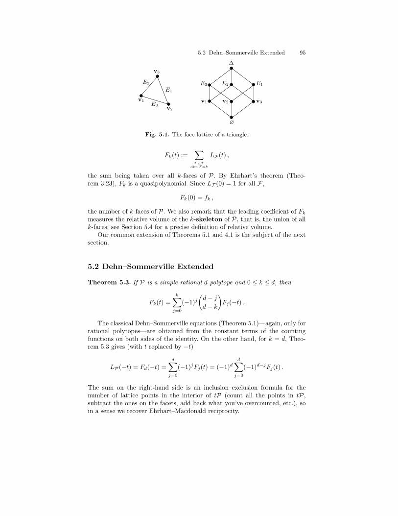
5.2 Dehn–Sommerville Extended 95
v1
v2
v3
E1
E2
E3
∅
v1 v2 v3
E3 E2 E1
∆
Fig. 5.1. The face lattice of a triangle.
Fk(t) :=∑F⊆P
dimF=k
LF (t) ,
the sum being taken over all k-faces of P. By Ehrhart’s theorem (Theo-rem 3.23), Fk is a quasipolynomial. Since LF (0) = 1 for all F ,
Fk(0) = fk ,
the number of k-faces of P. We also remark that the leading coefficient of Fkmeasures the relative volume of the k-skeleton of P, that is, the union of allk-faces; see Section 5.4 for a precise definition of relative volume.
Our common extension of Theorems 5.1 and 4.1 is the subject of the nextsection.
5.2 Dehn–Sommerville Extended
Theorem 5.3. If P is a simple rational d-polytope and 0 ≤ k ≤ d, then
Fk(t) =k∑j=0
(−1)j(d− jd− k
)Fj(−t) .
The classical Dehn–Sommerville equations (Theorem 5.1)—again, only forrational polytopes—are obtained from the constant terms of the countingfunctions on both sides of the identity. On the other hand, for k = d, Theo-rem 5.3 gives (with t replaced by −t)
LP(−t) = Fd(−t) =d∑j=0
(−1)jFj(t) = (−1)dd∑j=0
(−1)d−jFj(t) .
The sum on the right-hand side is an inclusion–exclusion formula for thenumber of lattice points in the interior of tP (count all the points in tP,subtract the ones on the facets, add back what you’ve overcounted, etc.), soin a sense we recover Ehrhart–Macdonald reciprocity.

96 5 Face Numbers and the Dehn–Sommerville Relations in Ehrhartian Terms
Proof. Suppose F is a k-face of P. Then, again by counting the integer pointsin F according to relatively open faces of F ,
LF (t) =∑G⊆F
LG◦(t) ,
or, by the Ehrhart–Macdonald reciprocity (Theorem 4.1),
LF (t) =∑G⊆F
(−1)dimGLG(−t) =k∑j=0
(−1)j∑G⊆F
dimG=j
LG(−t) . (5.1)
Now sum both left- and right-hand sides over all k-faces and rearrange thesum on the right-hand side:
Fk(t) =∑F⊆P
dimF=k
k∑j=0
(−1)j∑G⊆F
dimG=j
LG(−t)
=k∑j=0
(−1)j∑F⊆P
dimF=k
∑G⊆F
dimG=j
LG(−t)
=k∑j=0
(−1)j∑G⊆P
dimG=j
fk(P/G)LG(−t)
=k∑j=0
(−1)j∑G⊆P
dimG=j
(d− jd− k
)LG(−t)
=k∑j=0
(−1)j(d− jd− k
)Fj(−t) .
Here fk(P/G) denotes the number of k-faces of P containing a given j-face Gof P. Since P is simple, this number equals
(d−jd−k)
(see Exercise 5.4). ut
5.3 Applications to the Coefficients of an EhrhartPolynomial
We will now apply Theorem 5.3 to the computation of the Ehrhart polynomialof an integral d-polytope P. The only face-lattice-point enumerator involvingthe face P is Fd(t), for which Theorem 5.3 specializes to
LP(t) = Fd(t) =d∑j=0
(−1)jFj(−t) .

5.3 Applications to the Coefficients of an Ehrhart Polynomial 97
In fact, we do not have to assume that P is simple, since this identity simplycounts integer points by faces. (Recall that (−1)jFj(−t) counts the integerpoints in the t-dilates of the interior of the j-faces.)5 The last term on theright-hand side is
(−1)dFd(−t) = (−1)dLP(−t) = LP◦(t)
by Ehrhart–Macdonald reciprocity. Shifting this term to the left gives
LP(t)− LP◦(t) =d−1∑j=0
(−1)jFj(−t) . (5.2)
The difference on the left-hand side of this identity has a natural interpre-tation: it counts the integer points on the boundary of tP. (And in fact, theright-hand side is once more an inclusion–exclusion formula for this num-ber.) Let us write LP(t) = cd t
d + cd−1 td−1 + · · · + c0. Then LP◦(t) =
cd td − cd−1 t
d−1 + · · ·+ (−1)dc0, so that
LP(t)− LP◦(t) = 2cd−1 td−1 + 2cd−3 t
d−3 + · · · ,
where this sum ends with 2c0 if d is odd and 2c1t if d is even (this should lookfamiliar; see Exercise 4.10). Combining this expression with (5.2) yields thefollowing useful result.
Theorem 5.4. Suppose LP(t) = cd td + cd−1 t
d−1 + · · · + c0 is the Ehrhartpolynomial of P. Then
cd−1 td−1 + cd−3 t
d−3 + · · · = 12
d−1∑j=0
(−1)jFj(−t) . ut
We can make the statement of this theorem more precise (but also moremessy) by writing
Fj(t) =∑F⊆P
dimF=j
LF (t) = cj,j tj + cj,j−1t
j−1 + · · ·+ cj,0 .
Then collecting the coefficients of tk in Theorem 5.4 yields the following rela-tions.
Corollary 5.5. If k and d are of different parity, then
ck =12
d−1∑j=0
(−1)j+kcj,k . ut
5 So one might argue that we did not need the Dehn–Sommerville machinery forthe computations in the current section. This argument is correct, although The-orem 5.3 is a strong motivation.
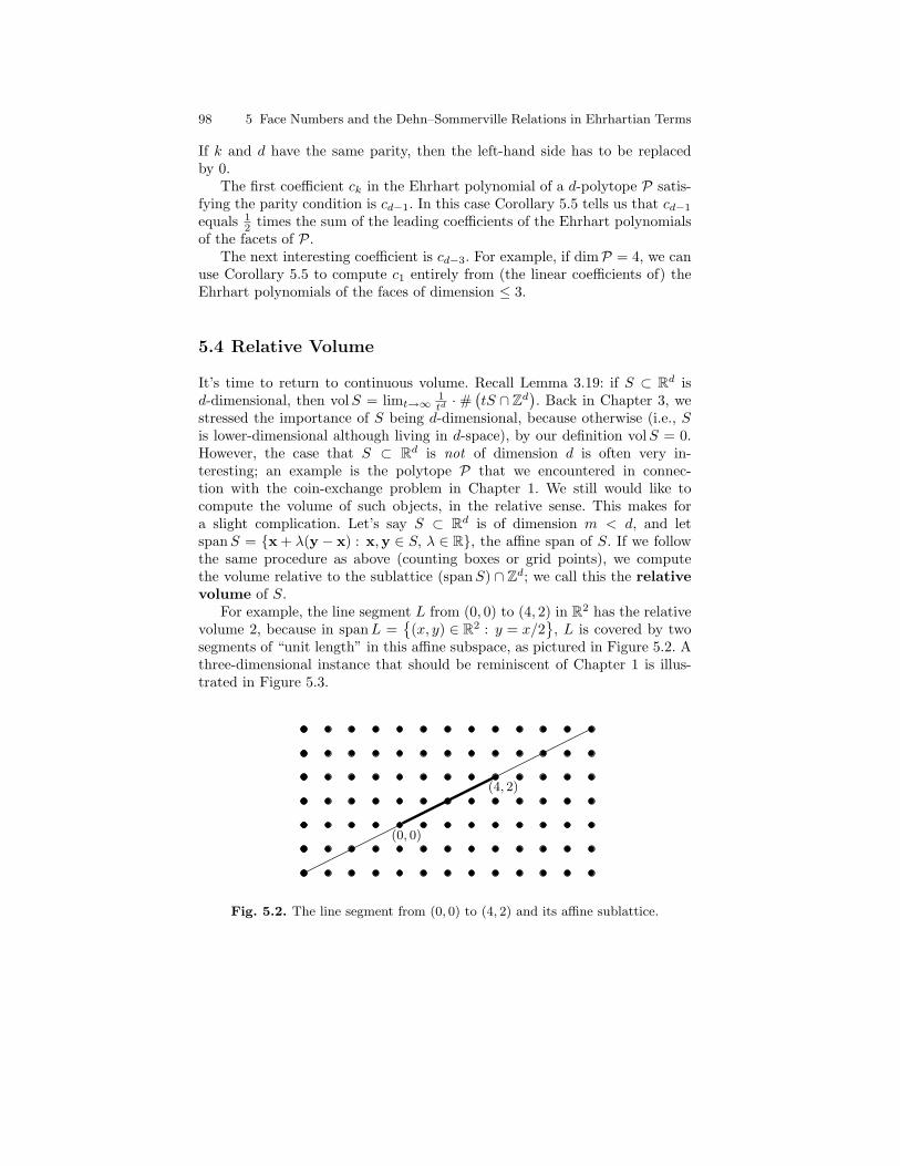
98 5 Face Numbers and the Dehn–Sommerville Relations in Ehrhartian Terms
If k and d have the same parity, then the left-hand side has to be replacedby 0.
The first coefficient ck in the Ehrhart polynomial of a d-polytope P satis-fying the parity condition is cd−1. In this case Corollary 5.5 tells us that cd−1
equals 12 times the sum of the leading coefficients of the Ehrhart polynomials
of the facets of P.The next interesting coefficient is cd−3. For example, if dimP = 4, we can
use Corollary 5.5 to compute c1 entirely from (the linear coefficients of) theEhrhart polynomials of the faces of dimension ≤ 3.
5.4 Relative Volume
It’s time to return to continuous volume. Recall Lemma 3.19: if S ⊂ Rd isd-dimensional, then volS = limt→∞
1td·#(tS ∩ Zd
). Back in Chapter 3, we
stressed the importance of S being d-dimensional, because otherwise (i.e., Sis lower-dimensional although living in d-space), by our definition volS = 0.However, the case that S ⊂ Rd is not of dimension d is often very in-teresting; an example is the polytope P that we encountered in connec-tion with the coin-exchange problem in Chapter 1. We still would like tocompute the volume of such objects, in the relative sense. This makes fora slight complication. Let’s say S ⊂ Rd is of dimension m < d, and letspanS = {x + λ(y − x) : x,y ∈ S, λ ∈ R}, the affine span of S. If we followthe same procedure as above (counting boxes or grid points), we computethe volume relative to the sublattice (spanS) ∩ Zd; we call this the relativevolume of S.
For example, the line segment L from (0, 0) to (4, 2) in R2 has the relativevolume 2, because in spanL =
{(x, y) ∈ R2 : y = x/2
}, L is covered by two
segments of “unit length” in this affine subspace, as pictured in Figure 5.2. Athree-dimensional instance that should be reminiscent of Chapter 1 is illus-trated in Figure 5.3.
(0, 0)
(4, 2)
Fig. 5.2. The line segment from (0, 0) to (4, 2) and its affine sublattice.

5.4 Relative Volume 99
2
20
5
x
y
z
Fig. 5.3. The triangle defined by x5
+ y20
+ z2
= 1, x ≥ 0, y ≥ 0, z ≥ 0. The shadedregion is a fundamental domain for the sublattice that lies on the affine span of thetriangle.
If S ⊆ Rd has full dimension d, the relative volume coincides with the“full-dimensional” volume. Henceforth, when we write volS we refer to therelative volume of S. With this convention we can rewrite Lemma 3.19 toaccommodate a set S ⊂ Rd that is m-dimensional: its relative volume can becomputed as
volS = limt→∞
1tm·#(tS ∩ Zd
).
In the case that #(tS ∩ Zd
)has the special form of a polynomial—for
example, if S is an integral polytope—we can further simplify this theorem.Suppose P ⊂ Rd is an integral m-polytope with Ehrhart polynomial
LP(t) = cm tm + cm−1 t
m−1 + · · ·+ c1 t+ 1 .
Then, according to the above discussion, and much in sync with Lemma 3.19,

100 5 Face Numbers and the Dehn–Sommerville Relations in Ehrhartian Terms
volP = limt→∞
1tmLP(t) = lim
t→∞
cm tm + cm−1 t
m−1 + · · ·+ c1 t+ 1tm
= cm .
The relative volume of P is the leading term of the corresponding countingfunction LP .
For example, in the previous section we found that Corollary 5.5 impliesthat the second leading coefficient cd−1 of the Ehrhart polynomial of thed-polytope P equals 1
2 times the sum of the leading terms of the Ehrhartpolynomials of the facets of P. The leading term for one facet is simply therelative volume of that facet:
Theorem 5.6. Suppose LP(t) = cd td + cd−1 t
d−1 + · · · + c0 is the Ehrhartpolynomial of the integral polytope P. Then
cd−1 =12
∑F a facet of P
volF . ut
Notes
1. The Dehn–Sommerville relations (Theorem 5.1) first surfaced in the workof Max Dehn, who proved them in 1905 for dimension five [71]. (The Dehn–Sommerville relations are not that complicated for d ≤ 4; see Exercise 5.3.)Some two decades later, D. M. Y. Sommerville proved the general case [167].Theorem 5.1 was neither well known nor much used in the first half of thetwentieth century, but only after its rediscovery by Victor Klee [111] and itsappearance in Branko Grunbaum’s famous and widely read book [90].
2. The Euler relation (Theorem 5.2) is easy to prove directly for d = 3 (thiscase is attributed to Euler), but for higher dimension, one has to be somewhatcareful, as we already remarked in the text. The classical proof for general dwas found in 1852 by Ludwig Schlafli [158], although it (like numerous laterproofs) assumes that the boundary of a convex polytope can be built upinductively in a “good” way. This nontrivial fact—which is called shelling ofa polytope—was proved by Heinz Bruggesser and Peter Mani in 1971 [50].Shellability is nicely discussed in [193, Lecture 8]. There are short proofs ofthe Euler relation that do not use the shelling of a polytope (see, for example,[120, 139, 184]).
3. The reader might suspect that proving Theorems 5.1 and 5.2 for rationalpolytopes suffices for the general case, since it seems that we can transforma polytope with irrational vertices slightly to one with only rational verticeswithout changing the face structure of the polytope. This is true in our every-day world but fails in dimension ≥ 4 (see [156] for dimension 4 and [193,pp. 172/173] for general dimension).

Exercises 101
4. Theorem 5.3 is due to Peter McMullen [127], who, in fact, proved this resultin somewhat greater generality. Another generalization of Theorem 5.3 can befound in [59].
Exercises
5.1. Consider a simple 3-polytope with at least five facets. Two players playthe following game: Each player, in turn, signs his or her name on a previouslyunsigned face. The winner is the player who first succeeds in signing threefacets that share a common vertex. Show that the player who signs first willalways win by playing as well as possible.6
5.2. Show that for the d-cube, fk = 2d−k(dk
).
5.3. Give an elementary proof of the Dehn–Sommerville relations (Theo-rem 5.1) for d ≤ 4.
5.4. ♣ Let P be a simple d-polytope. Prove that the number of k-faces of Pcontaining a given j-face of P equals
(d−jd−k).
5.5. ♣ Show directly, without using Theorem 5.2, that for a d-simplex:
(a) fk =(d+1k+1
).
(b)d∑k=0
(−1)kfk = 1.
5.6. Prove Theorem 5.1 directly (and hence not requiring P to be an integralpolytope). (Hint: Orient yourself along the proof of Theorem 5.3, but startwith the Euler relation (Theorem 5.2) for a given face F instead of (5.1).)
5.7. Let F be a face of a simple polytope P. Prove that∑G⊇F
(−1)dimG(
dimGk
)= (−1)d
(dimFd− k
), k = 0, . . . , d.
5.8. Show that the equations in Theorem 5.3 are equivalent to the followingidentities. If P is a simple lattice d-polytope and k ≤ d, then
k∑j=0
(−1)k−j(d− jk − j
)Fd−j(−n) =
d∑i=k
(−1)i−k(i
k
)Fi(n) .
6 This was one of the 2002 Putnam contest problems.

102 5 Face Numbers and the Dehn–Sommerville Relations in Ehrhartian Terms
5.9. Prove that the equations in the previous exercise imply the followingidentities which compare the number of lattice points in faces and relativeinteriors of faces of the simple polytope P:
k∑j=0
(−1)j(d− jk − j
) ∑F⊆P
dimF=d−j
#(F ∩ Zd
)=
d∑i=k
(i
k
) ∑G⊆P
dimG=i
#(G◦ ∩ Zd
),
where k = 0, . . . , d = dimP. For example, for k = 0, we have
#(P ∩ Zd) =∑G⊆P
#(G◦ ∩ Zd
),
and for k = d we obtain the inclusion–exclusion formula
#(P◦ ∩ Zd) =d∑j=0
(−1)d−j∑F⊆P
dimF=j
#(F ∩ Zd
).
5.10. Another nice reformulation of Theorem 5.3 is the following generalizedreciprocity law. For a simple integral d-polytope P, define the generalizedEhrhart polynomial
Ek(t) :=k∑j=0
(−1)j(d− jk − j
) ∑F⊆P
dimF=d−j
LF (t) , k = 0, . . . , d.
Prove the generalized reciprocity law
Ek(−t) = (−1)dEd−k(t) , k = 0, . . . , d,
which implies Ehrhart–Macdonald reciprocity (Theorem 4.1) when k = 0.
5.11. What happens when P is not simple? Give an example for which The-orem 5.3 fails.
5.12. Give an alternative proof of Theorem 5.6 by considering LP(t)−LP◦(t)as the lattice-point enumerator of the boundary of P.

6
Magic Squares
The peculiar interest of magic squares and all lusus numerorum in general lies inthe fact that they possess the charm of mystery.
W. S. Andrews
Fig. 6.1. Magic square at the Temple de la Sagrada Famılia (Barcelona, Spain).
Equipped with a solid base of theoretical results, we are now ready to returnto computations. We use Ehrhart theory to assist us in enumerating magicsquares.
Loosely speaking, a magic square is an n × n array of integers (usuallyrequired to be positive, often restricted to the numbers 1, 2, . . . , n2, usuallyrequired to have distinct entries) whose sum along any row, column, and maindiagonal is the same number, called the magic sum. Magic squares have turned

104 6 Magic Squares
up time and again, some in mathematical contexts, others in philosophical orreligious contexts. According to legend, the first magic square (the ancient LuoShu square) was discovered in China sometime before the first century B.C.E.on the back of a turtle emerging from a river. It was the square pictured inFigure 6.2.
4 9 2
3 5 7
8 1 6
Fig. 6.2. The Luo Shu square.
Our task in this chapter is to develop a theory for counting certain classesof magic squares, which we now introduce.
6.1 It’s a Kind of Magic
One should notice that the Luo Shu square has the distinct entries 1, 2, . . . , 9,so these entries are positive, distinct integers drawn from a particular set. Suchrequirements are too restrictive for our purposes. We define a semimagicsquare to be a square matrix whose entries are nonnegative integers andwhose rows and columns (called lines in this setting) sum to the same number.A magic square is a semimagic square whose main diagonals also add up tothe line sum. Figure 6.3 shows two examples.
3 0 0
0 1 2
0 2 1
1 2 0
0 1 2
2 0 1
Fig. 6.3. A semimagic and a magic square.
We caution the reader about clashing definitions in the literature. Forexample, some people reserve the term “magic square” for what we will calla traditional magic square, a magic square of order n whose entries arethe distinct integers 1, 2, . . . , n2. (The Luo Shu square is an example of atraditional magic square.) Others are slightly less restrictive and use the term

6.1 It’s a Kind of Magic 105
“magic square” for a magic square with distinct entries. We stress that we donot make this requirement in this chapter.
Our goal is to count semimagic and magic squares. In the traditional case,this is in some sense not very interesting:1 for each order there is a fixednumber of traditional magic squares. For example, there are 7040 traditional4× 4 magic squares.
The situation becomes more interesting if we drop the condition of tra-ditionality and study the number of magic squares as a function of the linesum. We denote the total numbers of semimagic and magic squares of ordern and line sum t by Hn(t) and Mn(t), respectively.
♥ t−♥
t−♥ ♥
t
2
t
2
t
2
t
2
Fig. 6.4. Semimagic and magic squares for n = 2.
Example 6.1. We illustrate these notions for the case n = 2, which is notvery complicated. Here a semimagic square is determined once we know oneentry, say the upper left one, denoted by ♥ in Figure 6.4. Because of the upperrow sum, the upper right entry has to be t − ♥, as does the lower left entry(because of the left column sum). But then the lower right entry has to bet − (t − ♥) = ♥ (for two reasons: the lower row sum and the right columnsum). The entry ♥ can be any integer between 0 and t. Since there are t+ 1such integers,
H2(t) = t+ 1 . (6.1)
In the magic case, we also have to think of the diagonals. Looking back at oursemimagic square in Figure 6.4, the first diagonal gives 2 · ♥ = t, or ♥ = t/2.In this case, t − ♥ = t/2, and so a 2 × 2 magic square has to have identicalentries in each position. Because we require the entries to be integers, this ispossible only if t is even, in which case we obtain precisely one solution, thesquare on the right in Figure 6.4. That is,
M2(t) ={
1 if t is even,0 if t is odd.
These easy results already hint at something: the counting function Hn is ofa different character than the function Mn. ut1 It is, nevertheless, an incredibly hard problem to count all traditional magic
squares of a given size n. At present, these numbers are known only for n ≤ 5[165, Sequence A006052].

106 6 Magic Squares
6.2 Semimagic Squares: Integer Points in theBirkhoff–von Neumann Polytope
Just as the Frobenius problem was intrinsically connected to questions aboutinteger points on line segments, triangles, and higher-dimensional simplices,magic squares and their relatives have a life in the world of geometry. Themost famous example is connected to semimagic squares.
A semimagic n×n square has n2 nonnegative entries that sum to the samenumber along any row or column. Consider therefore the polytope
Bn :=
x11 · · · x1n
......
xn1 . . . xnn
∈ Rn2
: xjk ≥ 0,∑j xjk = 1 for all 1 ≤ k ≤ n∑k xjk = 1 for all 1 ≤ j ≤ n
,
(6.2)consisting of nonnegative real matrices, in which all rows and columns sumto one. Bn is called the nth Birkhoff–von Neumann polytope, in honorof Garrett Birkhoff (1911–1996)2 and John von Neumann (1903–1957).3 Be-cause the matrices contained in the Birkhoff–von Neumann polytope appearfrequently in probability and statistics (the line sum 1 representing probabil-ity 1), Bn is often described as the set of all n× n doubly stochastic matrices.
Geometrically, Bn is a subset of Rn2and as such difficult to picture once
n exceeds 1.4 However, we can get a glimpse of B2 ⊂ R4 when we think aboutwhat form points in B2 can possibly attain. Very much in sync with Figure 6.4,such a point is determined by its upper left entry ♥, pictured in Figure 6.5.This entry ♥ is a real number between 0 and 1, which suggests that B2 should
„♥ 1−♥
1−♥ ♥
«
Fig. 6.5. A point in B2.
look like a line segment in 4-space. Indeed, the vertices of B2 should be givenby ♥ = 0 and ♥ = 1, that is, by the points(
1 00 1
),
(0 11 0
)∈ B2 .
2 For more information about Birkhoff, seehttp://www-groups.dcs.st-and.ac.uk/∼history/Mathematicians/Birkhoff Garrett.html.
3 For more information about von Neumann, seehttp://www-groups.dcs.st-and.ac.uk/∼history/Mathematicians/Von Neumann.html.
4 The case n = 1 is not terribly interesting: B1 = {1} is a point.
6.2 Semimagic Squares: Points in the Birkhoff–von Neumann Polytope 107
These results generalize: Bn is an (n− 1)2-polytope (see Exercise 6.3), whosevertices (Exercise 6.5) are the permutation matrices, namely, those n× nmatrices that have precisely one 1 in each row and column (every other entrybeing zero). For dimensional reasons, we can talk about the continuous volumeof Bn only in the relative sense, following the definition of Section 5.4.
The connection of the semimagic counting function Hn(t) to the Birkhoff–von Neumann polytope Bn becomes clear in the light of the lattice-point enu-merator for Bn: the counting function Hn(t) enumerates precisely the integerpoints in tBn, that is,
Hn(t) = #(tBn ∩ Zn
2)
= LBn(t) .
We can say more after noticing that permutation vertices are integer pointsin Bn, and so Ehrhart’s theorem (Theorem 3.8) applies:
Theorem 6.2. Hn(t) is a polynomial in t of degree (n− 1)2. ut
The fact that Hn is a polynomial—apart from being mathematicallyappealing—has the same nice computational consequence that we exploitedin Section 3.6: we can calculate this counting function by interpolation. Forexample, to compute H2, a linear polynomial, we need to know only two val-ues. In fact, since we know that the constant term of H2 is 1 (by Corollary3.15), we need only one value. It is not hard to convince even a lay personthat H2(1) = 2 (which two semimagic squares are those?), from which weinterpolate
H2(t) = t+ 1 .
To interpolate the polynomial H3, we need to know 4 values aside fromH3(0) = 1. In fact, we do not even have to know that many values, becauseEhrhart–Macdonald reciprocity (Theorem 4.1) assists us in computations. Tosee this, let H◦n(t) denote the number of n × n square matrices with positiveinteger entries summing up to t along each row and column. A moment’sthought (Exercise 6.6) reveals that
H◦n(t) = Hn(t− n) . (6.3)
But there is a second relationship between Hn and H◦n, namely, H◦n(t) counts,by definition, the integer points in the relative interior of the Birkhoff–vonNeumann polytope Bn, that is, H◦n(t) = LB◦n(t). Now Ehrhart–Macdonaldreciprocity (Theorem 4.1) gives
H◦n(−t) = (−1)(n−1)2Hn(t) .
Combining this identity with (6.3) gives us a symmetry identity for the count-ing function for semimagic squares:

108 6 Magic Squares
Theorem 6.3. The polynomial Hn satisfies
Hn(−n− t) = (−1)(n−1)2Hn(t)
andHn(−1) = Hn(−2) = · · · = Hn(−n+ 1) = 0 . ut
The roots of Hn at the first n − 1 negative integers follow from (Exer-cise 6.7)
H◦n(1) = H◦n(2) = · · · = H◦n(n− 1) = 0 .
Theorem 6.3 gives the degree of Bn, and it implies that the numerator of theEhrhart series of the Birkhoff–von Neumann polytope is palindromic:
Corollary 6.4. The Ehrhart series of the Birkhoff–von Neumann polytope Bnhas the form
EhrBn(z) =h(n−1)(n−2) z
(n−1)(n−2) + · · ·+ h0
(1− z)(n−1)2+1,
where h0, h1, . . . , h(n−1)(n−2) ∈ Z≥0 satisfy hk = h(n−1)(n−2)−k for 0 ≤ k ≤(n−1)(n−2)
2 .
Proof. Denote the Ehrhart series of Bn by
EhrBn(z) =h(n−1)2 z(n−1)2
+ · · ·+ h0
(1− z)(n−1)2+1.
The fact that h(n−1)2 = · · · = h(n−1)2−(n−2) = 0 follows from the secondpart of Theorem 6.3 and Theorem 4.5. The palindromy of the numeratorcoefficients follows from the first part of Theorem 6.3 and Exercise 4.7: itimplies
EhrBn
(1z
)= (−1)(n−1)2+1zn EhrBn(z) ,
which yields hk = h(n−1)(n−2)−k upon simplifying both sides of the equation.ut
Let’s return to the interpolation of H3: Theorem 6.3 gives, in addition toH3(0) = 1, the values
H3(−3) = 1 and H3(−1) = H3(−2) = 0 .
These four values together with H3(1) = 6 (see Exercise 6.1) suffice to inter-polate the quartic polynomial H3, and one computes
H3(t) =18t4 +
34t3 +
158t2 +
94t+ 1 . (6.4)

6.3 Magic Generating Functions and Constant-Term Identities 109
This interpolation example suggests the use of a computer; we let it calcu-late enough values of Hn and then simply interpolate. As far as computationsare concerned, however, we should not get too excited about the fact thatwe computed H2 and H3 so effortlessly. In general, the polynomial Hn hasdegree (n − 1)2, so we need to compute (n − 1)2 + 1 values of Hn to beable to interpolate. Of those, we know n (the constant term and the rootsgiven by Theorem 6.3), so n2 − 3n+ 2 values of Hn remain to be computed.Ehrhart–Macdonald reciprocity reduces the number of values to be computedto n2−3n+2
2 . That’s still a lot, as anyone can testify who has tried to get acomputer to enumerate all semimagic 7× 7 squares with line sum 15. Never-theless, it is a fun fact that we can compute Hn for small n by interpolation.It is amusing to test one’s computer against the constant-term computationwe will outline below, and we invite the reader to try both. For small n, in-terpolation is clearly superior to a constant-term computation in the spiritof Chapter 1. The turning point seems to be right around n = 5: the com-puter needs more and more time to compute the values Hn(t) as t increases.Methods superior to interpolation are needed.
6.3 Magic Generating Functions and Constant-TermIdentities
Now we will construct a generating function for Hn, for which we will useTheorem 2.13. The semimagic counting function Hn is the Ehrhart polynomialof the nth Birkhoff–von Neumann polytope Bn, which, in turn, is defined as aset of matrices by (6.2). First we rewrite the definition of Bn to fit the generaldescription (2.23) of a polytope. If we consider the points in Bn as columnvectors in Rn2
(rather than as matrices in Rn×n) then
Bn ={
x ∈ Rn2
≥0 : A x = b},
where
A =
1 · · · 11 · · · 1
. . .1 · · · 1
1 1 1. . . . . . · · ·
. . .1 1 1
∈ Z2n×n2
(6.5)
(here we omit the zero entries) and
b =
11...1
∈ Z2n.
110 6 Magic Squares
From this description of Bn, we can easily build the generating functionfor Hn. According to Theorem 2.13, for a general rational polytope P ={x ∈ Rd≥0 : A x = b
}, we have
LP(t) = const(
1(1− zc1) (1− zc2) · · · (1− zcd) ztb
),
where c1, c2, . . . , cd denote the columns of A. In our special case, the columnsof A are of a simple form: they contain exactly two 1’s and elsewhere 0’s. Weneed one generating-function variable for each row of A. To keep things asclear as possible, we use z1, z2, . . . , zn for the first n rows of A (representingthe row constraints of Bn) and w1, w2, . . . , wn for the last n rows of A (rep-resenting the column constraints of Bn). With this notation, Theorem 2.13applied to Bn gives the following starting point for our computations:
Theorem 6.5. The number Hn(t) of semimagic n× n squares with line sumt satisfies
Hn(t) = const
1∏1≤j,k≤n (1− zjwk)
(∏1≤j≤n zj
∏1≤k≤n wk
)t . ut
This identity is of both theoretical and practical use. One can use it to computeH3 and even H4 by hand. For now, we work on refining it further, exemplifiedby the case n = 2.
We first note that in the formula for H2, the variables w1 and w2 areseparated, in the sense that we can write this formula as a product of twofactors, one involving only w1 and the other involving only w2:
H2(t) = const(
1zt1z
t2
1(1− z1w1) (1− z2w1)wt1
1(1− z1w2) (1− z2w2)wt2
).
Now we put an ordering on the constant-term computation: let us first com-pute the constant term with respect to w2, then the one with respect to w1.(We don’t order the computation with respect to z1 and z2 just yet.) Since z1,z2, and w1 are considered constants when we do constant-term computationswith respect to w2, we can simplify:
H2(t) = constz1,z2
(1
zt1zt2
constw1
(1
(1− z1w1) (1− z2w1)wt1
× constw2
(1
(1− z1w2) (1− z2w2)wt2
))).
Now we can see the effect of the separate appearance of w1 and w2: theconstant-term identity factors. This is very similar to the factoring that canappear in computations of integrals in several variables. Let us rewrite ouridentity to emphasize the factoring:

6.3 Magic Generating Functions and Constant-Term Identities 111
H2(t) = constz1,z2
(1
zt1zt2
constw1
(1
(1− z1w1) (1− z2w1)wt1
)× constw2
(1
(1− z1w2) (1− z2w2)wt2
)).
But now the expressions in the last two sets of parentheses are identical,except that in one case the constant-term variable is called w1 and in theother case w2. Since these are just “dummy” variables, we can call them w,and combine:
H2(t) = constz1,z2
(1
zt1zt2
(constw
1(1− z1w) (1− z2w)wt
)2).
(Note the square!) Naturally, all of this factoring works in the general case,and we invite the reader to prove it (Exercise 6.8):
Hn(t) = constz1,...,zn
((z1 · · · zn)−t
(constw
1(1− z1w) · · · (1− znw)wt
)n).
(6.6)We can go further, namely, we can compute the innermost constant term
constw1
(1− z1w) · · · (1− znw)wt.
It should come as no surprise that we’ll use a partial fraction expansion to doso. The w-poles of the rational function are at w = 1/z1, w = 1/z2, . . . , w =1/zn, w = 0, and so we expand
1(1− z1w) · · · (1− znw)wt
=A1
w − 1z1
+A2
w − 1z2
+· · ·+ An
w − 1zn
+t∑
k=1
Bkwk
. (6.7)
Just as in Chapter 1, we can forget about the Bk-terms, since they do notcontribute to the constant term, that is,
constw1
(1− z1w) · · · (1− znw)wt
= constw
(A1
w − 1z1
+A2
w − 1z2
+ · · ·+ An
w − 1zn
)= −A1z1 −A2z2 − · · · −Anzn .
We invite the reader to show (Exercise 6.9) that
Ak = −zt−1k(
1− z1zk
)· · ·(
1− zk−1zk
)(1− zk+1
zk
)· · ·(
1− znzk
)= −
zt+n−2k∏
j 6=k(zk − zj). (6.8)

112 6 Magic Squares
Putting these coefficients back into the partial fraction expansion yields thefollowing identity.
Theorem 6.6. The number Hn(t) of semimagic n× n squares with line sumt satisfies
Hn(t) = const
((z1 · · · zn)−t
(n∑k=1
zt+n−1k∏
j 6=k(zk − zj)
)n). ut
Amidst all this generality, we almost forgot to compute H2 with our partialfraction approach. The last theorem says that
H2(t) = const
((z1z2)−t
(zt+1
1
z1 − z2+
zt+12
z2 − z1
)2)
= const(
zt+21 z−t2
(z1 − z2)2− 2
z1z2
(z1 − z2)2+
z−t1 zt+22
(z1 − z2)2
). (6.9)
Now it’s time to put more order on the constant-term computation. Let’s saywe first compute the constant term with respect to z1, and after that withrespect to z2. So we have to compute first
constz1
(zt+2
1 z−t2
(z1 − z2)2
), constz1
(z1z2
(z1 − z2)2
), and constz1
(z−t1 zt+2
2
(z1 − z2)2
).
To obtain these constant terms, we need to expand the function 1(z1−z2)2 . As
we know from calculus, this expansion depends on the order of the magnitudesof z1 and z2. For example, if |z1| < |z2| then
1z1 − z2
=1z2
1z1z2− 1
= − 1z2
∑k≥0
(z1
z2
)k= −
∑k≥0
1zk+1
2
zk1 ,
and hence
1(z1 − z2)2
= − d
dz1
(1
z1 − z2
)=∑k≥1
k
zk+12
zk−11 =
∑k≥0
k + 1zk+2
2
zk1 .
So let’s assume for the moment that |z1| < |z2|. This might sound funny, sincez1 and z2 are variables. However, as such they are simply tools that enableus to compute some quantity that is independent of z1 and z2. In view ofthese ideas, we may assume any order of the magnitudes of the variables. InExercise 6.11 we will check that indeed the order does not matter. Now,
6.3 Magic Generating Functions and Constant-Term Identities 113
constz1
(zt+2
1 z−t2
(z1 − z2)2
)= z−t2 constz1
(zt+2
1
(z1 − z2)2
)
= z−t2 constz1
zt+21
∑k≥0
k + 1zk+2
2
zk1
(6.10)
= z−t2 constz1
∑k≥0
k + 1zk+2
2
zk+t+21
= 0 ,
since there are only positive powers of z1 (remember that t ≥ 0). Analogously(see Exercise 6.10) one checks that
constz1
(z1z2
(z1 − z2)2
)= 0 . (6.11)
For the last constant term, we compute
constz1
(z−t1 zt+2
2
(z1 − z2)2
)= zt+2
2 constz1
z−t1
∑k≥0
k + 1zk+2
2
zk1
= zt+2
2 constz1
∑k≥0
k + 1zk+2
2
zk−t1
.
The constant term on the right-hand side is the term with k = t, that is,
constz1
(z−t1 zt+2
2
(z1 − z2)2
)= zt+2
2
t+ 1zt+2
2
= t+ 1 .
So of the three constant terms only one survives, and with constz2(t+1) = t+1we recover what we have known since the beginning of this chapter:
H2(t) = const(
zt+21 z−t2
(z1 − z2)2− 2
z1z2
(z1 − z2)2+
z−t1 zt+22
(z1 − z2)2
)= t+ 1 .
This was a lot of work for this seemingly trivial polynomial. Recall, forexample, that we can get the same result by an easy interpolation. How-ever, to compute a similar interpolation, e.g., for H4, we likely would needto use a computer (to obtain the interpolation values). On the other hand,the constant-term computation of H4 boils down to only five iterated con-stant terms, which can actually be computed by hand (see Exercise 6.14).The result is
H4(t) =11
11340t9 +
11630
t8 +19135
t7 +23t6 +
1109540
t5 +4310t4 +
351175670
t3
+37963
t2 +6518t+ 1 .

114 6 Magic Squares
6.4 The Enumeration of Magic Squares
What happens when we bring the diagonal constraints, which are not presentin the semimagic case, into the magic picture? In the introduction of thischapter we have already seen an example, namely the number of 2× 2 magicsquares,
M2(t) ={
1 if t is even,0 if t is odd.
This is a very simple example of a quasipolynomial. In fact, like Hn, thecounting function Mn is defined by integral linear equations and inequalities,so it is the lattice-point enumerator of a rational polytope, and Theorem 3.23gives at once the following result.
Theorem 6.7. The counting function Mn(t) is a quasipolynomial in t. ut
We invite the reader to prove that the degree of Mn is n2 − 2n − 1 (Exer-cise 6.16).
Let’s see what happens in the first nontrivial case, 3 × 3 magic squares.We follow our recipe and assign variables m1,m2, . . . ,m9 to the entries of our3× 3 squares, as in Figure 6.6.
m1 m2 m3
m4 m5 m6
m7 m8 m9
Fig. 6.6. Variables in a magic 3× 3 square.
The magic conditions require now that m1,m2, . . . ,m9 ∈ Z≥0 and
m1 +m2 +m3 = t ,
m4 +m5 +m6 = t ,
m7 +m8 +m9 = t ,
m1 +m4 +m7 = t ,
m2 +m5 +m8 = t ,
m3 +m6 +m9 = t ,
m1 +m5 +m9 = t ,
m3 +m5 +m7 = t ,
according to the row sums (the first three equations), the column sums (thenext three equations), and the diagonal sums (the last two equations). By
Notes 115
now, we’re experienced in translating this system into a generating function:we need one variable for each equation, so let’s take z1, z2, z3 for the firstthree, w1, w2, w3 for the next three, and y1, y2 for the last two equations. Thefunction M3(t) is the constant term of
1(1− z1w1y1) (1− z1w2) (1− z1w3y2) (1− z2w1) (1− z2w2y1y2) (1− z2w3)
× 1(1− z3w1y2) (1− z3w2) (1− z3w3y1) (z1z2z3w1w2w3y1y2)t
. (6.12)
It does take some work, but it is instructive to compute this constant term(just try it!). The result is
M3(t) =
{29 t
2 + 23 t+ 1 if 3|t,
0 otherwise.(6.13)
As predicted by Theorem 6.7, M3 is a quasipolynomial. It has degree 2 andperiod 3. This may be more apparent if we rewrite it as
M3(t) =
29 t
2 + 23 t+ 1 if t ≡ 0 mod 3,
0 if t ≡ 1 mod 3,0 if t ≡ 2 mod 3,
and we can see the three constituents of the quasipolynomial M3. There isan alternative way to describe M3; namely, let
c2(t) =
29 if t ≡ 0 mod 3,0 if t ≡ 1 mod 3,0 if t ≡ 2 mod 3,
c1(t) =
23 if t ≡ 0 mod 3,0 if t ≡ 1 mod 3,0 if t ≡ 2 mod 3,
c0(t) =
1 if t ≡ 0 mod 3,0 if t ≡ 1 mod 3,0 if t ≡ 2 mod 3.
Then the quasipolynomial M3 can be written as
M3(t) = c2(t) t2 + c1(t) t+ c0(t) .
Notes
1. Magic squares date back to China in the first millennium B.C.E. [53]; theyunderwent much further development in the Islamic world late in the first

116 6 Magic Squares
millennium C.E. and in the next millennium (or sooner; the data are lacking)in India [54]. From Islam they passed to Christian Europe in the later MiddleAges, probably initially through the Jewish community [54, Part II, pp. 290ff.] and later possibly Byzantium [54, Part I, p. 198], and no later than theearly eighteenth century (the data are buried in barely tapped archives) tosub-Saharan Africa [191, Chapter 12]. The contents of a magic square havevaried with time and writer; usually they have been the first n2 consecutiveintegers, but often any arithmetic sequence or arbitrary positive numbers.In the past century, mathematicians have made some simplifications in theinterest of obtaining results about the number of squares with a fixed magicsum, in particular, allowing repeated entries as in this chapter.
2. The problem of counting magic squares (other than traditional magicsquares) seems to have occurred to anyone only in the twentieth century,no doubt because there was no way to approach the question previously. Thefirst nontrivial formulas addressing the counting problem, namely (6.4) and(6.13) for H3 and M3, were established by Percy Macmahon (1854–1929)5
[124] in 1915. Recently there has grown up a literature on exact formulas (seefor example [80, 168] for semimagic squares; for magic squares see [1, 23]; formagic squares with distinct entries see [31, 189]).
3. Another famous kind of square is latin squares (see, for example, [72]).Here each row and column has n different numbers, the same n numbers inevery row/column (usually taken to be the first n positive integers). Thereare counting problems associated with latin squares, which can be attackedusing Ehrhart theory [31] (see also [165, Sequence A002860]).
4. Recent work includes mathematical-historical research, such as the discov-ery of unpublished magic squares of Benjamin Franklin [2, 141]. Aside frommathematical research, magic squares and their siblings naturally continueto be an excellent source of topics for popular mathematics books (see, forexample, [4] or [144]).
5. The Birkhoff–von Neumann polytope Bn possesses fascinating combinato-rial properties [38, 48, 49, 58, 192] and relates to many mathematical areas[74, 112]. Its name honors Garrett Birkhoff and John von Neumann, whoproved that the extremal points of Bn are the permutation matrices [39, 186](see Exercise 6.5). A long-standing open problem is the determination ofthe relative volume of Bn, which is known only for n ≤ 10 [165, SequenceA037302]. In fact, the last two records (n = 9 and 10) for computing volBnrely on the theory of counting functions that is introduced in this book, moreprecisely, Theorem 6.6 [28].
5 For more information about MacMahon, seehttp://www-groups.dcs.st-and.ac.uk/∼history/Mathematicians/MacMahon.html.

Exercises 117
6. An important generalization of the Birkhoff–von Neumann polytope is thetransportation polytopes, which consist of contingency tables. They have appli-cations to statistics and in particular to disclosure limitation procedures [68].The Birkhoff–von Neumann polytopes are special transportation polytopesthat consist of two-way contingency tables with given 1-marginals.
7. The polynomiality of Hn (Theorem 6.2) and its symmetry (Theorem 6.3)were conjectured in 1966 by Harsh Anand, Vishwa Dumir, and Hansraj Gupta[3] and proved seven years later independently by Eugene Ehrhart [80] andRichard Stanley [168]. Stanley also conjectured that the numerator coefficientsin Corollary 6.4 are unimodal, a fact that was proved only in 2005, by ChristosAthanasiadis [8]. The quasipolynomiality of Mn (Theorem 6.7) and its degreeare discussed in [23]. The period of Mn is in general not known. In [23] itis conjectured that it is always nontrivial for n > 1. The work in [1] givessome credence to this conjecture by proving that the polytope of magic n×nsquares is not integral for n ≥ 2.
8. We close with a story about Cornelius Agrippa’s De Occulta Philosophia,written in 1510. In it he describes the spiritual powers of magic squares andproduces some squares of orders from three up to nine. His work, althoughinfluential in the mathematical community, enjoyed only brief success, forthe Counter-Reformation and the witch hunts of the Inquisition began soonthereafter: Agrippa himself was accused of being allied with the devil.
Exercises
6.1. ♣ Find and prove a formula for Hn(1).
6.2. Let (xij)1≤i,j≤3 be a magic 3× 3 square.
(a) Show that the center term x22 is the average over all xij .(b) Show that M3(t) = 0 if 3 does not divide t.
6.3. ♣ Prove that dimBn = (n− 1)2.
6.4. Prove the following characterization of a vertex of a convex polytope P: Apoint v ∈ P is a vertex of P if for any line L through v and any neighborhoodN of v there exists a point in L ∩N that is not in P.
6.5. ♣ Prove that the vertices of Bn are the n× n-permutation matrices.
6.6. ♣ Let H◦n(t) denote the number of n × n matrices with positive integerentries summing up to t along each row and column. Show that H◦n(t) =Hn(t− n) for t > n.
6.7. ♣ Show that H◦n(1) = H◦n(2) = · · · = H◦n(n− 1) = 0.
118 6 Magic Squares
6.8. ♣ Prove (6.6):
Hn(t) = constz1,...,zn
((z1 · · · zn)−t
(constw
1(1− z1w) · · · (1− znw)wt
)n).
6.9. ♣ Compute the partial fraction coefficients (6.8).
6.10. ♣ Verify (6.11).
6.11. Repeat the constant-term computation of H2 starting from (6.9), butnow by first computing the constant term with respect to z2, and after thatwith respect to z1.
6.12. Use your favorite computer program to calculate the formula for H3(t),H4(t), . . . by interpolation.
6.13. Compute H3 using Theorem 6.6.
6.14. Compute H4 using Theorem 6.6.
6.15. Show thatn∑k=1
zt+n−1k∏
j 6=k(zk − zj)=
∑m1+···+mn=t
zm11 · · · zmnn ,
and use this identity to give an alternative proof of Theorem 6.6.
6.16. ♣ Prove that for n ≥ 3, the degree of Mn is n2 − 2n− 1.
6.17. Compute the vertices of the polytope of 3× 3 magic squares.
6.18. ♣ Verify (6.12) and use it to compute M3.
6.19. Compute M3 by interpolation. (Hint: Use Exercises 6.2 and 6.17.)
6.20. A symmetric semimagic square is a semimagic square that is a sym-metric matrix. Show that the number of symmetric semimagic n× n squareswith line sum t is a quasipolynomial in t. Determine its degree and period.
Open Problems
6.21. Compute the number of traditional magic n× n squares for n > 5.
6.22. Compute volBn for n > 10. Compute Hn for n > 9.
6.23. Prove that the period of Mn is nontrivial for n > 1.
6.24. The vertices of the Birkhoff–von Neumann polytope are in one-to-onecorrespondence with the elements of the symmetric group Sn. Consider a sub-group of Sn and take the convex hull of the corresponding permutation matri-ces. Compute the Ehrhart polynomials of this polytope. (The face numbers ofthe polytope corresponding to the subgroup An, the even permutations, werestudied in [102].)
6.25. Prove that the graph formed by the vertices and edges of any 2-waytransportation polytope is Hamiltonian.
Part II
Beyond the Basics


7
Finite Fourier Analysis
God created infinity, and man, unable to understand infinity, created finite sets.
Gian-Carlo Rota (1932–1999)
We now consider the vector space of all complex-valued periodic functionson the integers with period b. It turns out that every such function a(n) onthe integers can be written as a polynomial in the bth root of unity ξn :=e2πin/b. Such a representation for a(n) is called a finite Fourier series.Here we develop the finite Fourier theory using rational functions and theirpartial fraction decomposition. We then define the Fourier transform and theconvolution of finite Fourier series, and show how one can use these ideas toprove identities on trigonometric functions, as well as find connections to theclassical Dedekind sums.
The more we know about roots of unity and their various sums, the deeperare the results that we can prove (see Exercise 7.19); in fact, certain statementsabout sums of roots of unity even imply the Riemann hypothesis! However,this chapter is elementary and draws connections to the sawtooth functionsand Dedekind sums, two basic sums over roots of unity. The general philos-ophy here is that finite sums of rational functions of roots of unity are basicingredients in many mathematical structures.
7.1 A Motivating Example
To ease the reader into the general theory, let’s work out the finite Fourierseries for a simple example first, an arithmetic function with a period of 3.
Example 7.1. Consider the following arithmetic function, of period 3:
n : 0, 1, 2, 3, 4, 5, . . .a(n) : 1, 5, 2, 1, 5, 2, . . .
122 7 Finite Fourier Analysis
We first embed this sequence into a generating function as follows:
F (z) := 1 + 5z + 2z2 + z3 + 5z4 + 2z5 + · · · =∑n≥0
a(n) zn.
Since the sequence is periodic, we can simplify F (z) using a geometric seriesargument:
F (z) =∑n≥0
a(n) zn
= 1 + 5z + 2z2 + z3(1 + 5z + 2z2
)+ z6
(1 + 5z + 2z2
)+ · · ·
=(1 + 5z + 2z2
)∑k≥0
z3k
=1 + 5z + 2z2
1− z3.
We now use the same technique that was employed in Chapter 1, namely thetechnique of expanding a rational function into its partial fraction decompo-sition. Here all the poles are simple, and located at the three cube roots ofunity, so that
F (z) =a(0)1− z
+a(1)
1− ρz+
a(2)1− ρ2z
, (7.1)
where the constants a(0), a(1), a(2) remain to be found, and where ρ := e2πi/3,a third root of unity. Using the geometric series for each of these terms sepa-rately, we arrive at
F (z) =∑n≥0
(a(0) + a(1)ρn + a(2)ρ2n
)zn,
so that we’ve derived the finite Fourier series of our sequence a(n)! The onlyremaining piece of information that we need is the computation of the con-stants a(j), for j = 0, 1, 2. It turns out that this is also quite easy to do. Wehave, from (7.1) above, the identity
a(0) (1− ρz)(1− ρ2z
)+ a(1) (1− z)
(1− ρ2z
)+ a(2) (1− z) (1− ρz)
= 1 + 5z + 2z2,
valid for all z ∈ C. Upon letting z = 1, ρ2, and ρ, respectively, we obtain
3 a(0) = 1 + 5 + 2 ,
3 a(1) = 1 + 5ρ2 + 2ρ4,
3 a(2) = 1 + 5ρ+ 2ρ2,
where we’ve used the identity (1− ρ)(1− ρ2) = 3 (see Exercise 7.2). We cansimplify a bit to get a(0) = 8
3 , a(1) = −4−3ρ3 , and a(2) = −1+3ρ
3 . Thus thefinite Fourier series for our sequence is

7.2 Finite Fourier Series for Periodic Functions on Z 123
a(n) =83
+(−4
3− ρ)ρn +
(−1
3+ ρ
)ρ2n. ut
The object of the next section is to show that this simple process follows justas easily for any periodic function on Z. The ensuing sections contain someapplications of the finite Fourier series of periodic functions.
7.2 Finite Fourier Series for Periodic Functions on Z
The general theory is just as easy conceptually as the example above, and wenow develop it. Consider any periodic sequence on Z, defined by {a(n)}∞n=0, ofperiod b. Throughout the chapter, we fix the bth root of unity ξ := e2πi/b. Asbefore, we embed our periodic sequence {a(n)}∞n=0 into a generating function,
F (z) :=∑n≥0
a(n) zn,
and use the periodicity of the sequence to immediately get
F (z) =
(b−1∑k=0
a(k) zk)
+
(b−1∑k=0
a(k) zk)zb +
(b−1∑k=0
a(k) zk)z2b + · · ·
=∑b−1k=0 a(k) zk
1− zb=
P (z)1− zb
,
where the last step simply defines the polynomial P (z) =∑b−1k=0 a(k) zk. Now
we expand the rational generating function F (z) into partial fractions, asbefore:
F (z) =P (z)
1− zb=
b−1∑m=0
a(m)1− ξmz
.
As in the example of the previous section, we expand each of the terms 11−ξmz
as a geometric series, and substitute into the sum above to get
F (z) =∑n≥0
a(n) zn =b−1∑m=0
a(m)1− ξmz
=b−1∑m=0
a(m)∑n≥0
ξmnzn =∑n≥0
(b−1∑m=0
a(m) ξmn)zn.
Comparing the coefficients of any fixed zn gives us the finite Fourier series fora(n), namely
a(n) =b−1∑m=0
a(m) ξmn.
124 7 Finite Fourier Analysis
We now find a formula for the Fourier coefficients a(n), as in the example.To recapitulate, we have
P (z) =b−1∑m=0
a(m)1− zb
1− ξmz.
To solve for P (ξ−n), we note that
limz→ξ−n
1− zb
1− ξmz= 0 if m− n 6≡ 0 mod b,
and
limz→ξ−n
1− zb
1− ξmz= limz→ξ−n
bzb−1
ξm= b ξn−m = b if m− n ≡ 0 mod b.
Thus P (ξ−n) = b a(n) and so
a(n) =1bP (ξ−n) =
1b
b−1∑k=0
a(k) ξ−nk.
We have just proved the main result of finite Fourier series, using only ele-mentary properties of rational functions:
Theorem 7.2 (Finite Fourier series expansion and Fourier inver-sion). Let a(n) be any periodic function on Z, with period b. Then we havethe following finite Fourier series expansion:
a(n) =b−1∑k=0
a(k) ξnk,
where the Fourier coefficients are
a(n) =1b
b−1∑k=0
a(k) ξ−nk, (7.2)
with ξ = e2πi/b. ut
The coefficients a(m) are known as the Fourier coefficients of the func-tion a(n), and if a(m) 6= 0 we sometimes say that the function has fre-quency m. The finite Fourier series of a periodic function provides us withsurprising power and insight into its structure. We are able to analyze the func-tion using its frequencies (only finitely many), and this window into the fre-quency domain becomes indispensable for computations and simplifications.
We note that the Fourier coefficients a(n) and the original sequence ele-ments a(n) are related by a linear transformation given by the matrix

7.2 Finite Fourier Series for Periodic Functions on Z 125
L =(ξ(i−1)(j−1)
), (7.3)
where 1 ≤ i, j ≤ b, as is evident from (7.2) in the proof above. We further notethat the second half of the proof, namely solving for the Fourier coefficientsa(n), is just tantamount to inverting this matrix L.
One of the main building blocks of our lattice-point enumeration formulasin polytopes is the sawtooth function, defined by
((x)) :=
{{x} − 1
2 if x /∈ Z,0 if x ∈ Z.
(7.4)
(As a reminder, {x} = x− bxc is the fractional part of x.) The graph of thisfunction is displayed in Figure 7.1. We have seen a closely related functionbefore, in Chapter 1, in our study of the coin-exchange problem. Equation(1.8) gave us the finite Fourier series for essentially this function from thediscrete-geometry perspective of the coin-exchange problem; however, we nowcompute the finite Fourier series for this periodic function directly, pretendingthat we do not know about its other life as a counting function.
x
y
Fig. 7.1. The sawtooth function y = ((x)).
Lemma 7.3. The finite Fourier series for the discrete sawtooth function((ab
)), a periodic function of a ∈ Z with period b, is given by
((ab
))=
12b
b−1∑k=1
1 + ξk
1− ξkξak =
i
2b
b−1∑k=1
cotπk
bξak.
Here the second equality follows from 1+e2πix
1−e2πix = i cot(πx), by the definitionof the cotangent.
Proof. Using Theorem 7.2, we know that our periodic function has a finiteFourier series
((ab
))=∑b−1k=0 a(k) ξak, where

126 7 Finite Fourier Analysis
a(k) =1b
b−1∑m=0
((mb
))ξ−mk.
We first compute a(0) = 1b
∑b−1m=0
((mb
))= 0, by Exercise 7.14. For k 6= 0, we
have
a(k) =1b
b−1∑m=1
(m
b− 1
2
)ξ−mk =
1b2
b−1∑m=1
mξ−mk +12b
=1b
(ξk
1− ξk+
12
)=
12b
1 + ξk
1− ξk,
where we used Exercise 7.5 in the penultimate equality above. ut
We define the Dedekind sum by
s(a, b) =b−1∑k=0
((ka
b
))((k
b
)),
for any two relatively prime integers a and b > 0. Note that the Dedekindsum is a periodic function of the variable a, with period b, by the periodicityof the sawtooth function. That is,
s(a+ jb, b) = s(a, b) for all j ∈ Z . (7.5)
Using the finite Fourier series for the sawtooth function, we can now easilyreformulate the Dedekind sums as a finite sum over the bth roots of unity orcotangents:
Lemma 7.4.
s(a, b) =14b
b−1∑µ=1
1 + ξµ
1− ξµ1 + ξ−µa
1− ξ−µa=
14b
b−1∑µ=1
cotπµ
bcot
πµa
b.
Proof.
s(a, b) =b−1∑k=0
((ka
b
))((k
b
))
=1
4b2
b−1∑k=0
((b−1∑µ=1
1 + ξµ
1− ξµξµka
)(b−1∑ν=1
1 + ξν
1− ξνξνk
))
=1
4b2
b−1∑µ=1
b−1∑ν=1
1 + ξµ
1− ξµ1 + ξν
1− ξν
(b−1∑k=0
ξk(ν+µa)
).
We note that the last sum∑b−1k=0 ξ
k(ν+µa) vanishes, unless ν ≡ −µa mod b(Exercise 7.6), in which case the sum equals b, and we obtain

7.3 The Finite Fourier Transform and Its Properties 127
s(a, b) =14b
b−1∑µ=1
1 + ξµ
1− ξµ1 + ξ−µa
1− ξ−µa.
Rewriting the right-hand side in terms of cotangents gives
s(a, b) =i2
4b
b−1∑µ=1
cotπµ
bcot−πµab
=14b
b−1∑µ=1
cotπµ
bcot
πµa
b,
because the cotangent is an odd function. ut
7.3 The Finite Fourier Transform and Its Properties
Given a periodic function f on Z, we have seen that f possesses a finiteFourier series, with the finite collection of Fourier coefficients that we calledf(0), f(1), . . . , f(b − 1). We now regard f as a function on the finite setG = {0, 1, 2, . . . , b− 1}, and let VG be the vector space of all complex-valuedfunctions on G. Equivalently, VG is the vector space of all complex-valued,periodic functions on Z with period b.
We define the Fourier transform of f , denoted by F(f), to be the peri-odic function on Z defined by the sequence of uniquely determined values
f(0), f(1), . . . , f(b− 1) .
ThusF(f)(m) = f(m) .
Theorem 7.2 above gave us these coefficients as a linear combination of thevalues f(k), with k = 0, 1, 2, . . . , b − 1. Thus F(f) is a linear transformationof the function f , thought of as a vector in VG. In other words, we’ve shownthat F(f) is a one-to-one and onto linear transformation of VG.
The vector space VG is a vector space of dimension b; indeed, an explicitbasis can easily be given for VG using the “delta functions” (see Exercise 7.7)defined by
δm(x) :=
{1 if x = m+ kb, for some integer k,0 otherwise.
In other words, δm(x) is the periodic function on Z that picks out the arith-metic progression {m+ kb : k ∈ Z}.
But there is another natural basis for VG. For any fixed integer a the rootsof unity {ea(x) := e2πiax/b : x ∈ Z} can be thought of as a single functionea(x) ∈ VG because of its periodicity on Z. As we saw in Theorem 7.2, thefunctions {e1(x), . . . , eb(x)} give a basis for the vector space of functions VG.A natural question now arises: how are the two bases related to each other?An initial observation is

128 7 Finite Fourier Analysis
δa(n) =1be−2πian/b,
which simply follows from the computation
δa(n) =1b
b−1∑k=0
δa(k) ξ−kn =1bξ−an =
1be−2πian/b.
So to get from the first basis to the second basis, we need precisely the finiteFourier transform!
It is extremely useful to define the following inner product on this vectorspace:
〈f, g〉 =b−1∑k=0
f(k) g(k) , (7.6)
for any two functions f, g ∈ VG. Here the bar denotes complex conjugation.The following elementary properties show that 〈f, g〉 is an inner product (seeExercise 7.8):
1. 〈f, f〉 ≥ 0, with equality if and only if f = 0, the zero function.2. 〈f, g〉 = 〈g, f〉.
Equipped with this inner product, VG can now be regarded as a metricspace. We can now measure distances between any two functions, and inparticular between any two basis elements ea(x) := e2πiax/b and ec(x) :=e2πicx/b. Any positive definite inner product gives rise to the distance functiond(f, g) = 〈f − g, f − g〉.
Lemma 7.5 (Orthogonality relations).
1b〈ea, ec〉 = δa(c) =
{1 if b | (a− c),0 otherwise.
Proof. We compute the inner product
〈ea, ec〉 =b−1∑m=0
ea(m) ec(m) =b−1∑m=0
e2πi(a−c)m/b.
If b | (a− c), then each term equals 1 in the latter sum, and hence the sumequals b. This verifies the first case of the lemma.
If b - (a− c), then ea−c(m) = e2πim(a−c)/b is a nontrivial root of unity, andwe have the finite geometric series
b−1∑m=0
e2πi(a−c)m
b =eb
2πi(a−c)b − 1
e2πi(a−c)
b − 1= 0 ,
verifying the second case of the lemma. ut

7.4 The Parseval Identity 129
Example 7.6. We recall the sawtooth function again, since it is one of thebuilding blocks of lattice point enumeration, and compute its Fourier trans-form. Namely, we define
B(k) :=((
k
b
))=
{{kb
}− 1
2 if kb /∈ Z,
0 if kb ∈ Z,
a periodic function on the integers with period b. What is its finite Fouriertransform? We have already seen the answer, in the course of the proof ofLemma 7.3:
B(n) =12b
1 + ξn
1− ξn=
i
2bcot
πn
b
for n 6= 0, and B(0) = 0. As always, ξ = e2πi/b. utIn the next section we delve more deeply into the behavior of this inner
product, where the Parseval identity is proved.
7.4 The Parseval Identity
A nontrivial property of the inner product defined above is the following iden-tity, linking the “norm of a function” to the “norm of its Fourier transform.” Itis known as the Parseval identity, and also goes by the name of the Planchereltheorem.
Theorem 7.7 (Parseval identity). For all f ∈ VG,
〈f, f〉 = b 〈f , f〉 .
Proof. Using the definition em(x) = ξmx and the relation
f(x) =1b
b−1∑m=0
f(m) em(x)
from Theorem 7.2, we have
〈f , f〉 =
⟨1b
b−1∑m=0
f(m) em ,1b
b−1∑n=0
f(n) en
⟩
=1b2
b−1∑k=0
b−1∑m=0
f(m) em(k)b−1∑n=0
f(n) en(k)
=1b2
b−1∑m=0
b−1∑n=0
f(m) f(n) 〈em, en〉
=1b
b−1∑m=0
b−1∑n=0
f(m) f(n) δm(n)
=1b〈f, f〉 ,
130 7 Finite Fourier Analysis
where the essential step in the proof was using the orthogonality relations(Lemma 7.5) in the fourth equality above. ut
A basically identical proof yields the following stronger result, showing thatthe “distance between any two functions” is essentially equal to the “distancebetween their Fourier transforms.”
Theorem 7.8. For all f, g ∈ VG, we have
〈f, g〉 = b 〈f , g〉 . ut
Example 7.9. A nice application of the generalized Parseval identity abovenow gives us Lemma 7.4 very quickly, the reformulation of the Dedekind sumas a sum over roots of unity. Namely, we first fix an integer a relatively primeto b and define f(k) =
((kb
)), and g(k) =
((kab
)). Then, using Example 7.6, we
have f(n) = i2b cot πnb . To find the Fourier transform of g we need an extra
twist. Since ((ka
b
))=
i
2b
b−1∑m=1
cotπm
bξmka,
we can multiply each index m by a−1, the multiplicative inverse of a modulob (recall that we require a and b to be relatively prime for the reformulationof the Dedekind sum). Since a−1 is relatively prime to b, this multiplicationjust permutes m = 1, 2, . . . , b − 1 modulo b, but the sum stays invariant (seeExercise 1.9):
b−1∑m=1
cotπm
bξmka =
b−1∑m=1
cotπma−1
bξma
−1ka =b−1∑m=1
cotπma−1
bξmk,
that is,
g(n) =i
2bcot
πna−1
b.
Hence Theorem 7.8 immediately gives us the reformulation of the Dedekindsum:
s(a, b) :=b−1∑k=0
((k
b
))((ka
b
))
= b
b−1∑m=1
(i
2bcot
πm
b
)(i
2bcot
πma−1
b
)
=14b
b−1∑m=1
cotπm
bcot
πma−1
b
=14b
b−1∑m=1
cotπma
bcot
πm
b.
For the last equality, we again used the trick of replacing m by ma. ut

7.5 The Convolution of Finite Fourier Series 131
7.5 The Convolution of Finite Fourier Series
Another basic tool in finite Fourier analysis is the convolution of two finiteFourier series. Namely, suppose f and g are periodic functions with period b.We define the convolution of f and g by
(f ∗ g)(t) =b−1∑m=0
f(t−m)g(m) .
Indeed, it is this convolution tool (the proof of the convolution theorem be-low is almost trivial!) that is responsible for the fastest known algorithm formultiplying two polynomials of degree b in O(b log(b)) steps (see the Notes atthe end of this chapter).
Theorem 7.10 (Convolution theorem for finite Fourier series). Letf(t) = 1
b
∑b−1k=0 ak ξ
kt and g(t) = 1b
∑b−1k=0 ck ξ
kt, where ξ = e2πi/b. Then theirconvolution satisfies
(f ∗ g)(t) =1b
b−1∑k=0
akck ξkt.
Proof. The proof is straightforward: we just compute the left-hand side, andobtain
b−1∑m=0
f(t−m)g(m) =1b2
b−1∑m=0
(b−1∑k=0
ak ξk(t−m)
)(b−1∑l=0
cl ξlm
)
=1b2
b−1∑k=0
b−1∑l=0
akcl
(b−1∑m=0
ξkt+(l−k)m
)
=1b
b−1∑k=0
akck ξkt,
because the sum∑b−1m=0 ξ
(l−k)m vanishes, unless l = k (see Exercise 7.6). Inthe case that l = k, we have
∑b−1m=0 ξ
(l−k)m = b. ut
It is an easy exercise (Exercise 7.22) to show that this convolution theoremis equivalent to the following statement:
F(f ∗ g) = bF(f)F(g) .
Note that the proof of Theorem 7.10 is essentially identical with the proof ofLemma 7.4 above; we could have proved the lemma, in fact, by applying theconvolution theorem. We now show how Theorem 7.10 can be used to deriveidentities on trigonometric functions.

132 7 Finite Fourier Analysis
Example 7.11. We claim that
b−1∑k=1
cot2
(πk
b
)=
(b− 1)(b− 2)3
.
The sum suggests the use of the convolution theorem, with a function whoseFourier coefficients are ak = ck = cot πkb . But we already know such a function!It is just the sawtooth function 2b
i
((mb
)). Therefore
− 14b
b−1∑k=1
cot2
(πk
b
)ξkt =
b−1∑m=1
((t−mb
))((mb
)),
where the equality follows from Theorem 7.10. On setting t = 0, we obtain
b−1∑m=1
((−mb
))((mb
))= −
b−1∑m=1
((mb
))((mb
))= − 1
b2
b−1∑m=1
m2 +1b
b−1∑m=1
m− 14
(b− 1)
= − (b− 1)(b− 2)12b
,
as desired. We used the identity((−m
b
))= −
((mb
))in the first equality above,
and some algebra was used in the last equality. Notice, moreover, that theconvolution theorem gave us more than we asked for, namely an identity forevery value of t. ut
Notes
1. Finite Fourier analysis offers a wealth of applications and is, for example,one of the main tools in quantum information theory. For the reader inter-ested in going further than the humble beginnings outlined in this chapter,we heartily recommend Audrey Terras’s monograph [180].
2. The Dedekind sum is our main motivation for studying finite Fourier series,and in fact, Chapter 8 is devoted to a detailed investigation of these sums, inwhich the Fourier–Dedekind sums of Chapter 1 also finally reappear.
3. The reader may consult [116, p. 501] for a proof that two polynomials ofdegree N can be multiplied in O(N logN) steps. The proof of this fact runsalong the following conceptual lines. First, let the two given polynomials ofdegree N be f(x) =
∑Nn=0 a(n)xn and g(x) =
∑Nn=0 b(n)xn. Then we know
that f(ξ) and g(ξ) are two finite Fourier series, and we abbreviate them by
Exercises 133
f and g, respectively. We now note that fg = F(F−1(f) ∗ F−1(g)). If wecan compute the finite Fourier transform (and its inverse) quickly, then thisargument shows that we can multiply polynomials quickly. It is a fact of lifethat we can compute the Fourier transform of a periodic function of periodN in O(N logN) steps, by an algorithm known as the fast Fourier transform(again, see [116] for a complete description).
4. The continuous Fourier transform, defined by∫∞−∞ f(t)e−2πitxdt, can be
related to the finite Fourier transform in the following way. We approximatethe continuous integral by discretizing a large interval [0, a]. Precisely, we let∆ := a
b , and we let tk := k∆ = kab . Then∫ a
0
f(t)e−2πitxdt ≈b∑
k=1
f(tk)e−2πitkxtk ,
a finite Fourier series for the function f(abx) as a function of x ∈ Z. Hencefinite Fourier series find an application to continuous Fourier analysis as anapproximation tool.
Exercises
Throughout the exercises, we fix an integer b > 1 and let ξ = e2πi/b.
7.1. Show that 1− xb =∏bk=1(1− ξkx).
7.2. ♣ Show that∏b−1k=1(1− ξk) = b.
7.3. Consider the matrix that came up in the proof of Theorem 7.2, namelyL = (aij), with aij := ξ(i−1)(j−1) and with 1 ≤ i, j ≤ b. Show that the matrix1√bL is a unitary matrix (recall that a matrix U is unitary if U∗U = I, where
U∗ is the conjugate transpose of U). Thus, this exercise shows that the Fouriertransform of a periodic function is always given by a unitary transformation.
7.4. Show that∣∣∣det
(1√bL)∣∣∣ = 1, where |z| denotes the norm of the complex
number z. (It turns out that det(L) can sometimes be a complex number, butwe will not use this fact here.)
7.5. ♣ For any integer a relatively prime to b, show that
1b
b−1∑k=1
k ξ−ak =ξa
1− ξa.
7.6. ♣ Let n be an integer. Show that the sum∑b−1k=0 ξ
kn vanishes, unlessn ≡ 0 (mod b), in which case it is equal to b.

134 7 Finite Fourier Analysis
7.7. ♣ For an integer m, define the delta function δm(x) by
δm(x) =
{1 if x = m+ ab, for some integer a,0 otherwise.
The b functions δ1(x), . . . , δb(x) are clearly in the vector space VG, since theyare periodic on Z with period b. Show that they form a basis for VG.
7.8. ♣ Prove that for all f, g ∈ VG:
(a) 〈f, f〉 ≥ 0, with equality if and only if f = 0, the zero function.(b) 〈f, g〉 = 〈g, f〉.
7.9. Show that∑b−1k=1
11−ξk = b−1
2 .
7.10. Show that 〈δa, δc〉 = δa(c).
7.11. Prove that (f ∗ δa)(x) = f(x− a).
7.12. Prove that δa ∗ δc = δ(a+c) mod b .
7.13. Let g(x) = x− a. Prove that f ◦ g = f(x) e2πiaxb .
7.14. ♣ For any real number x, prove that ((x)) =∑b−1k=0
((x+kb
)).
7.15. If x is not an integer, show that∑b−1n=0 cot
(π n+x
b
)= b cot (πx).
7.16. For any integer a relatively prime to b, show that∑ξ
ξa+1 − 1(ξa − 1)(ξ − 1)
= 0 ,
where the sum is taken over all bth roots of unity ξ except ξ = 1.
7.17. We call a root of unity e2πia/b a primitive bth root of unity if a isrelatively prime to b. Let Φb(x) denote the polynomial with leading coefficient1 and of degree φ(b)1 whose roots are the φ(b) distinct primitive bth roots ofunity. This polynomial is known as the cyclotomic polynomial of order b. Showthat ∏
d|b
Φd(x) = xb − 1 ,
where the product is taken over all positive divisors d of b.
1 φ(b) := # {k ∈ [1, b− 1] : gcd(k, b) = 1} is the Euler φ-function.

Exercises 135
7.18. We define the Mobius µ-function for positive integers n by
µ(n) =
1 if n = 1,0 if n is divisible by a square,(−1)k if n is square-free and has k prime divisors.
Deduce from the previous exercise that
Φb(x) =∏d|b
(xd − 1
)µ(b/d).
7.19. Prove that for any positive integer b,∑1≤a≤b, gcd(a,b)=1
e2πia/b = µ(b) ,
the Mobius µ-function.
7.20. Show that for any positive integer k, s(1, k) = − 14 + 1
6k + k12 .
7.21. Show that∑b−1k=1 tan2
(πkb
)= b(b− 1).
7.22. ♣ Show that Theorem 7.10 is equivalent to the following statement:
F(f ∗ g) = bF(f)F(g) .
7.23. Consider the trace of the linear transformation L =(ξ(i−1)(j−1)
), de-
fined in (7.3). The trace of L is G(b) :=∑b−1m=0 ξ
m2, known as a Gauß sum.
Show that |G(b)| =√b if b is an odd prime.


8
Dedekind Sums, the Building Blocks ofLattice-point Enumeration
If things are nice there is probably a good reason why they are nice: and if you don’tknow at least one reason for this good fortune, then you still have work to do.
Richard Askey
We’ve encountered Dedekind sums in our study of finite Fourier analysis andwe became intimately acquainted with their siblings in our study of the coin-exchange problem in Chapter 1. They have one shortcoming, however (whichwe’ll remove): the definition of s(a, b) requires us to sum over b terms, whichis rather slow when b = 2100, for example. Luckily, there is a magical reci-procity law for the Dedekind sum s(a, b) that allows us to compute it inroughly log2(b) = 100 steps. This is the kind of magic that saves the daywhen we try to enumerate lattice points in integral polytopes of dimensionsd ≤ 4. There is an ongoing effort to extend these ideas to higher dimensions,but there is much room for improvement. In this chapter we focus on thecomputational-complexity issues that arise when we try to compute Dedekindsums explicitely.
8.1 Fourier–Dedekind Sums and the Coin-ExchangeProblem Revisited
Recall from Chapter 1 the Fourier–Dedekind sum (defined in (1.13))
sn (a1, a2, . . . , ad; b) =1b
b−1∑k=1
ξknb(1− ξka1
b
)(1− ξka2
b
)· · ·(
1− ξkadb
) ,which appeared as a main player in our analysis of the Frobenius coin-exchange problem. We can now recognize the Fourier–Dedekind sums as hon-est finite Fourier series with period b. The Fourier–Dedekind sums unify many

138 8 Dedekind Sums
variations of the Dedekind sum that have appeared in the literature, and formthe building blocks of Ehrhart quasipolynomials. For example, we showed inChapter 1 that sn (a1, a2, . . . , ad; b) appears in the Ehrhart quasipolynomialof the d-simplex{
(x1, . . . , xd+1) ∈ Rd+1≥0 : a1x1 + · · ·+ adxd + bxd+1 = 1
}.
Example 8.1. We first notice that when n = 0 and d = 2, the Fourier–Dedekind sum reduces to a classical Dedekind sum (which—finally—explainsthe name): for relatively prime positive integers a and b,
s0(a, 1; b) =1b
b−1∑k=1
1(1− ξkab
) (1− ξkb
)=
1b
b−1∑k=1
(1
1− ξkab− 1
2
)(1
1− ξkb− 1
2
)
+12b
b−1∑k=1
11− ξkb
+12b
b−1∑k=1
11− ξkab
− 1b
b−1∑k=1
14
=14b
b−1∑k=1
(1 + ξkab1− ξkab
)(1 + ξkb1− ξkb
)+
1b
b−1∑k=1
11− ξkb
− b− 14b
.
In the last step we used the fact that multiplying the index k by a does notchange the middle sum. This middle sum can be further simplified by recalling(1.8):
1b
b−1∑k=1
1(1− ξkb
)ξknb
= −{nb
}+
12− 1
2b,
whence
s0(a, 1; b) =14b
b−1∑k=1
(1 + ξkab1− ξkab
)(1 + ξkb1− ξkb
)+
12− 1
2b− b− 1
4b
= − 14b
b−1∑k=1
cot(πka
b
)cot(πk
b
)+b− 1
4b(8.1)
= −s(a, b) +b− 1
4b. ut
Example 8.2. The next special evaluation of a Fourier–Dedekind sum is verysimilar to the computation above, so that we leave it to the reader to prove(Exercise 8.5) that for a1, a2 relatively prime to b,
s0 (a1, a2; b) = −s(a1a−12 , b
)+b− 1
4b, (8.2)
where a−12 a2 ≡ 1 mod b. ut

8.1 Fourier–Dedekind Sums and the Coin-Exchange Problem Revisited 139
Returning to the general Fourier–Dedekind sum, we now prove the firstof a series of reciprocity laws: identities for certain sums of Fourier–Dedekindsums. We first recall how these sums came up in Chapter 1, namely, from thepartial fraction expansion of the function
f(z) =1
(1− za1) · · · (1− zad) zn
=A1
z+A2
z2+ · · ·+ An
zn+
B1
z − 1+
B2
(z − 1)2+ · · ·+ Bd
(z − 1)d(8.3)
+a1−1∑k=1
C1k
z − ξka1
+a2−1∑k=1
C2k
z − ξka2
+ · · ·+ad−1∑k=1
Cdkz − ξkad
.
(Here we assume that a1, a2, . . . , ad are pairwise relatively prime.) Theo-rem 1.7 states that with the help of the partial fraction coefficients B1, . . . , Bdand Fourier–Dedekind sums, we can compute the restricted partition functionfor A = {a1, a2, . . . , ad}:
pA(n) = −B1 +B2 − · · ·+ (−1)dBd + s−n (a2, a3, . . . , ad; a1)+ s−n (a1, a3, a4, . . . , ad; a2) + · · ·+ s−n (a1, a2, . . . , ad−1; ad) .
We note that B1, B2, . . . , Bd are polynomials in n (Exercise 8.6), whence wecall
polyA(n) := −B1 +B2 − · · ·+ (−1)dBd
the polynomial part of the restricted partition function pA(n).
Example 8.3. The first few expressions for poly{a1,...,ad}(n) are
poly{a1}(n) =1a1,
poly{a1,a2}(n) =n
a1a2+
12
(1a1
+1a2
),
poly{a1,a2,a3}(n) =n2
2a1a2a3+n
2
(1
a1a2+
1a1a3
+1
a2a3
)(8.4)
+112
(3a1
+3a2
+3a3
+a1
a2a3+
a2
a1a3+
a3
a1a2
),
140 8 Dedekind Sums
poly{a1,a2,a3,a4}(n) =n3
6a1a2a3a4
+n2
4
(1
a1a2a3+
1a1a2a4
+1
a1a3a4+
1a2a3a4
)+n
4
(1
a1a2+
1a1a3
+1
a1a4+
1a2a3
+1
a2a4+
1a3a4
)+
n
12
(a1
a2a3a4+
a2
a1a3a4+
a3
a1a2a4+
a4
a1a2a3
)+
124
(a1
a2a3+
a1
a2a4+
a1
a3a4+
a2
a1a3+
a2
a1a4+
a2
a3a4
+a3
a1a2+
a3
a1a4+
a3
a2a4+
a4
a1a2+
a4
a1a3+
a4
a2a3
)+
18
(1a1
+1a2
+1a3
+1a4
). ut
We are about to combine the Ehrhart results of Chapter 3 with the partialfraction expansion of Chapter 1 that gave rise to the Fourier–Dedekind sums.
Theorem 8.4 (Zagier reciprocity). For any pairwise relatively prime pos-itive integers a1, a2, . . . , ad,
s0 (a2, a3, . . . , ad; a1) + s0 (a1, a3, a4, . . . , ad; a2) + · · ·+ s0 (a1, a2, . . . , ad−1; ad)
= 1− poly{a1,a2,...,ad}(0) .
At first sight, this reciprocity law should come as a surprise. The Fourier–Dedekind sums can be complicated, long sums, yet when combined in thisfashion, they add up to a trivial rational function in a1, a2, . . . , ad.
Proof. We compute the constant term of the quasipolynomial pA(n):
pA(0) = polyA(0) + s0 (a2, a3, . . . , ad; a1)+ s0 (a1, a3, a4, . . . , ad; a2) + · · ·+ s0 (a1, a2, . . . , ad−1; ad) .
On the other hand, Exercise 3.27 (the extension of Corollary 3.15 to Ehrhartquasipolynomials) states that pA(0) = 1, whence
1 = polyA(0) + s0 (a2, a3, . . . , ad; a1)+ s0 (a1, a3, a4, . . . , ad; a2) + · · ·+ s0 (a1, a2, . . . , ad−1; ad) . ut

8.2 The Dedekind Sum and Its Reciprocity and Computational Complexity 141
8.2 The Dedekind Sum and Its Reciprocity andComputational Complexity
We derived in (8.1) the classical Dedekind sum s(a, b) as a special evaluationof the Fourier–Dedekind sum. Naturally, Theorem 8.4 takes on a particularform when we specialize this reciprocity law to the classical Dedekind sum.
Corollary 8.5 (Dedekind’s reciprocity law). For any relatively primepositive integers a and b,
s(a, b) + s(b, a) =112
(a
b+b
a+
1ab
)− 1
4.
Proof. A special case of Theorem 8.4 is
s0(a, 1; b) + s0(b, a; 1) + s0(1, b; a) = 1− poly{a,1,b}(0)
= 1− 112
(3a
+ 3 +3b
+a
b+
1ab
+b
a
)=
34− 1
12
(a
b+b
a+
1ab
)− 1
4a− 1
4b.
Now we use the fact that s0(b, a; 1) = 0 and the identity (8.1):
s0(a, 1; b) = −s(a, b) +14− 1
4b. ut
Dedekind’s reciprocity law allows us to compute the Dedekind sum s(a, b)as quickly as the gcd algorithm for a and b. Let’s get a better feeling forthe way we can compute the Dedekind sum by working out an example. Weremind the reader of another crucial property of the Dedekind sums that wealready pointed out in (7.5): s(a, b) remains invariant when we replace a byits residue modulo b, that is,
s(a, b) = s(a mod b, b) . (8.5)
Example 8.6. Let a = 100 and b = 147. Now we alternately use Corollary 8.5and the reduction identity (8.5):
142 8 Dedekind Sums
s(100, 147) =112
(100147
+147100
+1
14700
)− 1
4− s(147, 100)
= − 124917640
− s(47, 100)
= − 124917640
−(
112
(47100
+10047
+1
4700
)− 1
4− s(100, 47)
)= − 773
20727+ s(6, 47)
= − 77320727
+112
(647
+476
+1
282
)− 1
4− s(47, 6)
=166441− s(5, 6)
=166441−(
112
(56
+65
+130
)− 1
4− s(6, 5)
)=
20034410
+ s(1, 5)
=20034410
− 14
+130
+512
=577882
.
In the last step we used Exercise 7.20: s(1, k) = − 14 + 1
6k + k12 . A priori,
s(100, 147) takes 147 steps to compute, whereas we were able to compute itin nine steps using Dedekind’s reciprocity law and (8.5). ut
As a second corollary to Theorem 8.4, we mention the following three-term reciprocity law for the special Fourier–Dedekind sum s0(a, b; c). Thisreciprocity law could be restated in terms of the classical Dedekind sum viathe identity (8.2).
Corollary 8.7. For pairwise relatively prime positive integers a, b, and c,
s0(a, b; c) + s0(c, a; b) + s0(b, c; a) = 1− 112
(3a
+3b
+3c
+a
bc+
b
ca+
c
ab
).
ut
8.3 Rademacher Reciprocity for the Fourier–DedekindSum
The next reciprocity law will be again for the general Fourier–Dedekind sums.It extends Theorem 8.4 beyond n = 0.
Theorem 8.8 (Rademacher reciprocity). Let a1, a2, . . . , ad be pairwiserelatively prime positive integers. Then for n = 1, 2, . . . , (a1 + · · ·+ ad − 1),

8.3 Rademacher Reciprocity for the Fourier–Dedekind Sum 143
sn (a2, a3, . . . , ad; a1) + sn (a1, a3, a4, . . . , ad; a2) + · · ·+ sn (a1, a2, . . . , ad−1; ad) = −poly{a1,a2,...,ad}(−n) .
Proof. We recall the definition
p◦A(n) = #{
(m1, . . . ,md) ∈ Zd : all mj > 0, m1a1 + · · ·+mdad = n}
of Exercise 1.31, that is, p◦A(n) counts the number of partitions of n usingonly the elements of A as parts, where each part is used at least once. Thiscounting function is, naturally, connected to pA through Ehrhart–Macdonaldreciprocity (Theorem 4.1):
p◦A(n) = (−1)d−1pA(−n) ,
that is,
(−1)d−1p◦A(n) = polyA(−n) + sn (a2, a3, . . . , ad; a1)+ sn (a1, a3, a4, . . . , ad; a2) + · · ·+ sn (a1, a2, . . . , ad−1; ad) .
On the other hand, by its very definition,
p◦A(n) = 0 for n = 1, 2, . . . , (a1 + · · ·+ ad − 1) ,
so that for those n,
0 = polyA(−n) + sn (a2, a3, . . . , ad; a1)+ sn (a1, a3, a4, . . . , ad; a2) + · · ·+ sn (a1, a2, . . . , ad−1; ad) . ut
Just as Zagier reciprocity takes on a special form for the classical Dedekindsum, Rademacher reciprocity specializes for d = 2 to a reciprocity identity forthe Dedekind–Rademacher sum
rn(a, b) :=b−1∑k=0
((ka+ n
b
))((k
b
)).
The classical Dedekind sum is, naturally, the specialization r0(a, b) = s(a, b).To be able to state the reciprocity law for the Dedekind–Rademacher sums,we define the function
χa(n) :=
{1 if a|n,0 otherwise,
which will come in handy as a book keeping device.
Corollary 8.9 (Reciprocity law for Dedekind–Rademacher sums).Let a and b be relatively prime positive integers. Then for n = 1, 2, . . . , a+ b,
144 8 Dedekind Sums
rn(a, b) + rn(b, a) =n2
2ab− n
2
(1ab
+1a
+1b
)+
112
(a
b+b
a+
1ab
)+
12
(((a−1n
b
))+((
b−1n
a
))+((na
))+((nb
)))+
14
(1 + χa(n) + χb(n)) ,
where a−1a ≡ 1 mod b and b−1b ≡ 1 mod a.
This identity follows almost instantly once we are able to express theDedekind–Rademacher sum in terms of Fourier–Dedekind sums.
Lemma 8.10. Suppose a and b are relatively prime positive integers and n ∈Z. Then
rn(a, b) = −sn(a, 1; b) +12
((nb
))+
12
((na−1
b
))− 1
4b+
14χb(n) ,
where a−1a ≡ 1 mod b.
Proof. We start by rewriting the finite Fourier series (1.8) for the sawtoothfunction ((x)):
1b
b−1∑k=1
ξknb1− ξkb
= −{−nb
}+
12− 1
2b
= −((−nb
))+
12χb(n)− 1
2b
=((nb
))+
12χb(n)− 1
2b.
Hence we also have
1b
b−1∑k=1
ξknb1− ξkab
=1b
b−1∑k=1
ξka−1n
b
1− ξkb
=((
a−1n
b
))+
12χb(a−1n
)− 1
2b
=((
a−1n
b
))+
12χb (n)− 1
2b.
Now we use the convolution theorem for finite Fourier series (Theorem 7.10)for the functions
f(n) :=1b
b−1∑k=1
ξknb1− ξkb
and g(n) :=1b
b−1∑k=1
ξknb1− ξkab
.
It gives
8.4 The Mordell–Pommersheim Tetrahedron 145
1b
b−1∑k=1
ξknb(1− ξkb
) (1− ξkab
) =b−1∑m=0
f(n−m) g(m) =
b−1∑m=0
(((n−mb
))+
12χb(n−m)− 1
2b
)(((a−1m
b
))+
12χb (m)− 1
2b
).
We invite the reader to check (Exercise 8.9) that the sum on the right-handside simplifies to
−b−1∑m=0
((am+ n
b
))((mb
))+
12
((a−1n
b
))+
12
((nb
))− 1
4b+
14χb(n) ,
whence
sn(a, 1; b) = −rn(a, b) +12
((a−1n
b
))+
12
((nb
))− 1
4b+
14χb(n) . ut
Proof of Corollary 8.9. We use the special case of Theorem 8.8
sn(a, 1; b) + sn(1, a; b) + sn(a, b; 1) = −poly{a,1,b}(−n)
= − n2
2ab+n
2
(1ab
+1a
+1b
)− 1
12
(3a
+3b
+ 3 +a
b+b
a+
1ab
),
which holds for n = 1, 2, . . . , a + b. Lemma 8.10 allows us to translate thisidentity into one for Dedekind–Rademacher sums:
rn(a, b) + rn(b, a) =n2
2ab− n
2
(1ab
+1a
+1b
)+
112
(a
b+b
a+
1ab
)+
12
(((a−1n
b
))+((
b−1n
a
))+((na
))+((nb
)))+
14
(1 + χa(n) + χb(n)) . ut
The two-term reciprocity law allows us to compute the Dedekind–Rade-macher sum as quickly as the gcd algorithm, just as obtained for the classicalDedekind sum. This fact has an interesting consequence: In Theorem 2.10and Exercise 2.34 we showed implicitly (see Exercise 8.10) that Dedekind–Rademacher sums are the only nontrivial ingredients of the Ehrhart quasipoly-nomials of rational polygons. Corollary 8.9 ensures that these Ehrhart quasi-polynomials can be computed almost instantly.
8.4 The Mordell–Pommersheim Tetrahedron
In this section we return to Ehrhart polynomials and illustrate how Dedekindsums appear naturally in generating-function computations. We will study

146 8 Dedekind Sums
the tetrahedron that historically first gave rise to the connection of Dedekindsums and lattice-point enumeration in polytopes. It is given by
P ={
(x, y, z) ∈ R3 : x, y, z ≥ 0,x
a+y
b+z
c≤ 1}, (8.6)
a tetrahedron with vertices (0, 0, 0), (a, 0, 0), (0, b, 0), and (0, 0, c), where a, b, care positive integers. We insert the slack variable n and interpret
LP(t) = #{
(k, l,m) ∈ Z3 : k, l,m ≥ 0,k
a+l
b+m
c≤ t}
= #{
(k, l,m, n) ∈ Z4 : k, l,m, n ≥ 0, bck + acl + abm+ n = abct}
as the Taylor coefficient of zabct for the function∑k≥0
zbck
∑l≥0
zacl
∑m≥0
zabm
∑n≥0
zn
=
1(1− zbc) (1− zac) (1− zab) (1− z)
.
As we have done numerous times before, we shift this coefficient to the con-stant term:
LP(t) = const(
1(1− zbc) (1− zac) (1− zab) (1− z) zabct
).
To reduce the number of poles, it is convenient to change this function slightly;the constant term of 1/
(1− zbc
)(1− zac)
(1− zab
)(1− z) is 1, so that
LP(t) = const(
z−abct − 1(1− zbc) (1− zac) (1− zab) (1− z)
)+ 1 .
This trick becomes useful in the next step, namely expanding the function intopartial fractions. Strictly speaking, we cannot do that, since the numeratoris not a polynomial in z. However, we can think of this rational function asa sum of two functions. The higher-order poles of both summands that wewill not include in our computation below cancel each other, so we can ignorethem at this stage. The only poles of
z−abct − 1(1− zbc) (1− zac) (1− zab) (1− z)
(8.7)
are at the ath, bth, cth roots of unity and at 0. (As before, we don’t haveto bother with the coefficients of z = 0 of the partial fraction expansion.) Tomake life momentarily easier (the general case is the subject of Exercise 8.12),let’s assume that a, b, and c are pairwise relatively prime; then all the polesbesides 0 and 1 are simple. The computation of the coefficients for z = 1 is
8.4 The Mordell–Pommersheim Tetrahedron 147
very similar to what we did with the restricted partition function in Chapter 1.The coefficient in the partial fraction expansion of a nontrivial root of unity,say ξka , is also computed practically as easily as in earlier examples: it is
− t
a (1− ξkbca ) (1− ξka)(8.8)
(see Exercise 8.11). Summing this fraction over k = 1, 2, . . . , a − 1 gives riseto the Fourier–Dedekind sum
− ta
a−1∑k=1
1(1− ξkbca ) (1− ξka)
= −t s0 (bc, 1; a) .
Putting this coefficient and its siblings for the other roots of unity into the par-tial fraction expansion and computing the constant term yields (Exercise 8.11)
LP(t) =abc
6t3 +
ab+ ac+ bc+ 14
t2
+(a+ b+ c
4+
14
(1a
+1b
+1c
)+
112
(bc
a+ca
b+ab
c+
1abc
))t
+ (s0 (bc, 1; a) + s0 (ca, 1; b) + s0 (ab, 1; c)) t+ 1 .
We recognize instantly that the Fourier–Dedekind sums in this Ehrhart poly-nomial are in fact classical Dedekind sums by (8.1), and so we arrive at thefollowing celebrated result.
Theorem 8.11. Let P be given by (8.6) with a, b, and c pairwise relativelyprime. Then
LP(t) =abc
6t3 +
ab+ ac+ bc+ 14
t2 +(
34
+a+ b+ c
4
+112
(bc
a+ca
b+ab
c+
1abc
)− s (bc, a)− s (ca, b)− s (ab, c)
)t+ 1 .
ut
We finish this chapter by giving the Ehrhart series of the Mordell–Pommersheim tetrahedron P. It follows simply from the transformation for-mulas (computing the Ehrhart numerator coefficients from the Ehrhart poly-nomial coefficients) of Corollary 3.16 and Exercise 3.10, and hence the Ehrhartseries of P naturally contains Dedekind sums.
Corollary 8.12. Let P be given by (8.6) with a, b, and c pairwise relativelyprime. Then
EhrP(z) =h3 z
3 + h2 z2 + h1 z + 1
(1− z)4,
148 8 Dedekind Sums
where
h3 =abc
6− ab+ ac+ bc+ a+ b+ c
4− 1
2+
112
(bc
a+ca
b+ab
c+
1abc
)− s (bc, a)− s (ca, b)− s (ab, c)
h2 =2abc
3+a+ b+ c
2+
32
+16
(bc
a+ca
b+ab
c+
1abc
)− 2 (s (bc, a) + s (ca, b) + s (ab, c))
h1 =abc
6+ab+ ac+ bc+ a+ b+ c
4− 2 +
112
(bc
a+ca
b+ab
c+
1abc
)− s (bc, a)− s (ca, b)− s (ab, c) . ut
It is a curious fact that the above expressions for h1, h2, and h3 are non-negative integers due to Corollary 3.11.
Notes
1. The classical Dedekind sums came to life in the 1880s when RichardDedekind (1831–1916)1 studied the transformation properties of the Dedekindη-function [70]
η(z) := eπiz/12∏n≥1
(1− e2πinz
),
a useful computational gadget in the land of modular forms in number theory.Dedekind’s reciprocity law (Corollary 8.5) follows from one of the functionaltransformation identities for η. Dedekind also proved that
12k s(h, k) ≡ k + 1− 2(h
k
)(mod 8) ,
establishing a beautiful connection between the Dedekind sum and the Jacobisymbol
(hk
)(the reader may want to consult the lovely Carus monograph
entitled Dedekind Sums, by Emil Grosswald and Hans Rademacher, where theabove result is proved [151, p. 34]), and then used this identity to show thatthe reciprocity law for the Dedekind sums (for which [151] contains severaldifferent proofs) is equivalent to the reciprocity law for the Jacobi symbol.
2. The Dedekind sums and their generalizations appear in various contexts be-sides analytic number theory and discrete geometry. Other mathematical areasin which Dedekind sums show up include topology [101, 131, 190], algebraicnumber theory [129, 166], and algebraic geometry [85]. They also have con-nections to algorithmic complexity [114] and continued fractions [10, 99, 138].1 For more information about Dedekind, seehttp://www-groups.dcs.st-and.ac.uk/∼history/Mathematicians/Dedekind.html.

Exercises 149
3. The reciprocity laws (Theorems 8.4 and 8.8) for the Fourier–Dedekindsums were proved in [25]. Theorem 8.4 is equivalent to the reciprocity law forDon Zagier’s higher-dimensional Dedekind sums [190]. Corollary 8.7 (statedin terms of the classical Dedekind sum) is originally due to Hans Rademacher[149]. Theorem 8.8 generalizes reciprocity laws by Rademacher [150] (essen-tially Corollary 8.9) and Ira Gessel [87].
4. The Fourier–Dedekind sums form only one set of generalizations of theclassical Dedekind sums. A long, but by no means complete, list of othergeneralizations is [5, 6, 21, 34, 35, 36, 56, 77, 78, 87, 92, 93, 113, 129, 131,130, 150, 179, 190].
5. The connection of Dedekind sums and lattice-point problems, namely The-orem 8.11 for t = 1, was first established by Louis Mordell in 1951 [136]. Some42 years later, James Pommersheim established a proof of Theorem 8.11 aspart of a much more general machinery [146]. In fact, Pommersheim’s workimplies that the classical Dedekind sum is the only nontrivial ingredient oneneeds for Ehrhart polynomials in dimensions three and four.
6. We touched the question of efficient computability of Ehrhart (quasi-)po-lynomials in this chapter. Unfortunately, our current state of knowledge ongeneralized Dedekind sums does not suffice to make any general statement.However, Alexander Barvinok proved in 1994 [15] that in fixed dimension,the rational generating function of the Ehrhart quasipolynomial of a ratio-nal polytope can be efficiently computed. Barvinok’s proof did not employDedekind sums but rather used a decomposition theorem of Brion, which isthe subject of Chapter 9.
Exercises
8.1. Show that s(a, b) = 0 if and only if a2 ≡ −1 mod b.
8.2. Prove that 6b s(a, b) ∈ Z. (Hint: Start with rewriting the Dedekind sumin terms of the greatest-integer function.)
8.3. Let a and b be any two relatively prime positive integers. Show that thereciprocity law for the Dedekind sums implies that for b ≡ r mod a,
12ab s(a, b) = −12ab s(r, a) + a2 + b2 − 3ab+ 1 .
Deduce the following identities:
(a) For b ≡ 1 mod a,
12ab s(a, b) = −a2b+ b2 + a2 − 2b+ 1 .

150 8 Dedekind Sums
(b) For b ≡ 2 mod a,
12ab s(a, b) = −12a2b+ a2 + b2 − 5
2b+ 1 .
(c) For b ≡ −1 mod a,
12ab s(a, b) = a2b+ a2 + b2 − 6ab+ 2b+ 1 .
8.4. Denote by fn the sequence of Fibonacci numbers, defined by
f1 = f2 = 1 and fn+2 = fn+1 + fn for n ≥ 1 .
Prove thats (f2k, f2k+1) = 0
and12f2k−1f2k s (f2k−1, f2k) = f2
2k−1 + f22k − 3f2k−1f2k + 1 .
8.5. ♣ Prove (8.2):
s0(a1, a2; b) = −s(a1a−12 , b
)+b− 1
4b,
where a−12 a2 ≡ 1 mod b.
8.6. Prove that B1, B2, . . . , Bd in the partial fraction expansion (8.3),
f(z) =1
(1− za1) · · · (1− zad) zn
=A1
z+A2
z2+ · · ·+ An
zn+
B1
z − 1+
B2
(z − 1)2+ · · ·+ Bd
(z − 1)d
+a1−1∑k=1
C1k
z − ξka1
+a2−1∑k=1
C2k
z − ξka2
+ · · ·+ad−1∑k=1
Cdkz − ξkad
,
are polynomials in n (of degree less than d) and rational functions in a1, . . . , ad.
8.7. ♣ Verify the first few expressions for poly{a1,...,ad}(n) in (8.4).
8.8. Show that the Dedekind–Rademacher sum satisfies r−n(a, b) = rn(a, b).
8.9. ♣ Show that
b−1∑m=0
(((n−mb
))+
12χb(n−m)− 1
2b
)(((a−1m
b
))+
12χb (m)− 1
2b
)
=b−1∑m=0
((am− n
b
))((mb
))+
12
((a−1n
b
))+
12
((−nb
))− 1
4b
+14χb(n) .

Open Problems 151
8.10. Rephrase the Ehrhart quasipolynomials for rational triangles given inTheorem 2.10 and Exercise 2.34 in terms of Dedekind–Rademacher sums.
8.11. ♣ Prove Theorem 8.11 by verifying (8.8) and computing the coefficientsfor z = 1 in the partial fraction expansion of (8.7).
8.12. Generalize the Ehrhart polynomial of the Mordell–Pommersheim tetra-hedron to the case that a, b, and c are not necessarily pairwise relativelyprime.
8.13. Compute the Ehrhart polynomial of the 4-simplex{(x1, x2, x3, x4) ∈ R4
≥0 :x1
a+x2
b+x3
c+x4
d≤ 1},
where a, b, c, d are pairwise relatively prime positive integers. (Hint: You mayuse Corollary 5.5 to compute the linear term.)
Open Problems
8.14. Find new relations between various Dedekind sums.
8.15. It is known [21] that the Fourier–Dedekind sums are efficiently com-putable. Find a fast algorithm that can be implemented in practice.
8.16. For any fixed integers b and k, find a nice characterization for the setof all a ∈ Z such that s(a, b) = k.

9
The Decomposition of a Polytope into ItsCones
Mathematics compares the most diverse phenomena and discovers the secret analo-gies that unite them.
Jean Baptiste Joseph Fourier (1768–1830)
In this chapter, we return to integer-point transforms of rational cones andpolytopes and connect them in a magical way that was first discovered byMichel Brion. The power of Brion’s theorem has been applied to various do-mains, such as Barvinok’s algorithm in integer linear programming, and tohigher-dimensional Euler–Maclaurin summation formulas, which we study inChapter 10. In a sense, Brion’s theorem is the natural extension of the familiarfinite geometric series identity
∑bm=a z
m = zb+1−zaz−1 to higher dimensions.
9.1 The Identity “∑
m∈Z zm = 0”. . .
. . . or “Much Ado About Nothing”
We start gently by illustrating Brion’s theorem in dimension one. To this end,let’s consider the line segment I := [20, 34]. We recall that its integer-pointtransform lists the lattice points in I in the form of monomials:
σI(z) =∑
m∈I∩Zzm = z20 + z21 + · · ·+ z34.
Already in this simple example, we are too lazy to list all integers in I anduse · · · to write the polynomial σI . Is there a more compact way to writeσI? The reader might have guessed it even before we asked the question: thisinteger-point transform equals the rational function
σI(z) =z20 − z35
1− z.

154 9 The Decomposition of a Polytope into Its Cones
This last sentence is not quite correct: the definition of σI(z) yielded a poly-nomial in z, whereas the rational function above is not defined at z = 1.We can overcome this deficiency by noticing that the limit of this rationalfunction as z → 1 equals the evaluation of the polynomials σI(1) = 15, byL’Hopital’s rule. Notice that the rational-function representation of σI hasthe unquestionable advantage of being much more compact than the originalpolynomial representation. The reader who is not convinced of this advantageshould replace the right vertex 34 of I by 3400.
Now let’s rewrite the rational form of the integer-point transform of Islightly:
σI(z) =z20 − z35
1− z=
z20
1− z+
z34
1− 1z
. (9.1)
There is a natural geometric interpretation of the two summands on the right-hand side. The first term represents the integer-point transform of the interval[20,∞):
σ[20,∞)(z) =∑m≥20
zm =z20
1− z.
The second term in (9.1) corresponds to the integer-point transform of theinterval (−∞, 34]:
σ(−∞,34](z) =∑m≤34
zm =z34
1− 1z
.
So (9.1) says that on a rational-function level,
σ[20,∞)(z) + σ(−∞,34](z) = σ[20,34](z) . (9.2)
This identity, which we illustrate graphically in Figure 9.1, should come
20 34
20 34
20 34
Fig. 9.1. Decomposing a line segment into two infinite rays.
as a mild surprise. Two rational functions that represent infinite sequencessomehow collapse, when being summed up, to a polynomial with a finitenumber of terms. We emphasize that (9.2) does not make sense on the level ofinfinite series; in fact, the two infinite series involved here have disjoint regionsof convergence.

9.1 The Identity “P
m∈Z zm = 0” . . . or “Much Ado About Nothing” 155
Even more magical is the geometry behind this identity: on the right-handside we have a polynomial that lists the integer points in a finite interval P,while on the left-hand side each of the rational generating functions representsthe integer points in an infinite ray that begins at a vertex of P. The twohalf-lines will be called vertex cones below, and indeed the remainder of thischapter is devoted to proving that an identity similar to (9.2) holds in generaldimension.
We now extend the definition of integer-point transforms σA(z) from thecase of cones A to the case of affine spaces A. Any such affine space A ⊆ Rdequals w + V for some w ∈ Rd and some n-dimensional vector subspaceV ⊆ Rd, and if A contains integer points (which is the only interesting casefor our purposes), we may choose w ∈ Zd. The integer points V ∩ Zd in Vform a Z-module, and hence there exists a basis v1,v2, . . . ,vn for V∩Zd. Thisimplies that any integer point m ∈ A ∩ Zd can be uniquely written as
m = w + k1v1 + k2v2 + · · ·+ knvn for some k1, k2, . . . , kn ∈ Z .
Using this fixed lattice basis for V, we define the skewed orthants of A as thesets of the form {w + λ1v1 + λ2v2 + · · ·+ λnvn}, where for each 1 ≤ j ≤ n,we require either λj ≥ 0 or λj < 0. So there are 2n such skewed orthants,and their disjoint union equals A. We denote them by O1,O2, . . . ,O2n . All ofthem are (half-open) pointed cones, and so their integer-point transforms arerational.
Lemma 9.1. Suppose A is an n-dimensional affine space with skewed or-thants O1,O2, . . . ,O2n . Then as rational functions,
σO1(z) + σO2(z) + · · ·+ σO2n (z) = 0 .
Proof. Suppose
A = {w + λ1v1 + λ2v2 + · · ·+ λnvn : λ1, λ2, . . . , λn ∈ R} .
Then a typical skewed orthant O looks like
O = {w + λ1v1 + λ2v2 + · · ·+ λnvn : λ1, . . . , λk ≥ 0, λk+1, . . . , λn < 0} ,
and its integer-point transform is
σO(z)
= zw
∑j1≥0
zj1v1
· · ·∑jk≥0
zjkvk
∑jk+1<0
zjk+1vk+1
· · ·∑jn<0
zjnvn
= zw 1
1− zv1· · · 1
1− zvk
1zvk+1 − 1
· · · 1zvn − 1
.
Now consider the skewed orthant O′ with the same conditions on the λ’s as inO except that we switch λ1 ≥ 0 to λ1 < 0. Then the integer-point transformof O′ is

156 9 The Decomposition of a Polytope into Its Cones
σO′(z) = zw 1zv1 − 1
11− zv2
· · · 11− zvk
1zvk+1 − 1
· · · 1zvn − 1
,
so that σO(z) + σO′(z) = 0. Since we can pair up all skewed orthants in thisfashion, the sum of all their rational generating functions is zero. ut
Since O1 ∪ O2 ∪ · · · ∪ O2n is equal to A as a disjoint union, it now makessense to set
σA(z) := 0 (9.3)
for any n-dimensional affine space with n > 0. Lemma 9.1 says that this defi-nition is not as arbitrary as it might seem, and the following result strengthensour motivation for the definition (9.3).
Theorem 9.2. Given half-open pointed cones K1,K2, . . . ,Km ⊆ Rd with acommon apex in Zd such that the disjoint union of K1,K2, . . . ,Km is an affinespace, then as rational functions,
σK1(z) + σK2(z) + · · ·+ σKm(z) = 0 .
Proof. Suppose the disjoint union of K1,K2, . . . ,Km is the n-dimensionalaffine space A, and w ∈ Zd is the common apex of K1,K2, . . . ,Km. Nowwe decompose A into the skewed orthants O1,O2, . . . ,O2n , which are alsopointed cones with common apex w. The intersection of one of the Kj ’s withone of the Ok’s is again a half-open pointed cone, and all these cones form yetanother disjoint union of A, which is a common refinement of the dissectionof A in terms of the Kj ’s and in terms of the Ok’s:
A =⋃
1≤j≤m1≤k≤2n
(Kj ∩ Ok) .
For each 1 ≤ j ≤ m, Kj =⋃2n
k=1 (Kj ∩ Ok) as a disjoint union, and so we canwrite the integer-point transform of Kj as
σKj (z) =2n∑k=1
σKj∩Ok(z) ,
as a rational-function identity. Similarly, we obtain for each 1 ≤ k ≤ 2n,
σOk(z) =m∑j=1
σKj∩Ok(z) .
Thus
m∑j=1
σKj (z) =m∑j=1
2n∑k=1
σKj∩Ok(z) =2n∑k=1
m∑j=1
σKj∩Ok(z) =2n∑k=1
σOk(z) = 0 ,
by Lemma 9.1. ut

9.2 Tangent Cones and Their Rational Generating Functions 157
9.2 Tangent Cones and Their Rational GeneratingFunctions
The goal of this section, apart from setting the language that allows us to proveBrion’s theorem, is to prove a sort of analogue of (9.2) in general dimension.
We recall a definition that was touched on only briefly, in Exercise 3.14:A hyperplane arrangement H is a finite collection of hyperplanes. Anarrangement H is rational if all its hyperplanes are, that is, if each hyper-plane in H is of the form
{x ∈ Rd : a1x1 + a2x2 + · · ·+ adxd = b
}for some
a1, a2, . . . , ad, b ∈ Z. An arrangement H is called a central hyperplane ar-rangement if its hyperplanes meet in (at least) one point.
Our next definition generalizes (finally) the notion of a pointed cone, de-fined in Chapter 3. A convex cone is the intersection of finitely many half-spaces of the form
{x ∈ Rd : a1x1 + a2x2 + · · ·+ adxd ≤ b
}for which the cor-
responding hyperplanes{x ∈ Rd : a1x1 + a2x2 + · · ·+ adxd = b
}form a cen-
tral arrangement. This definition extends that of a pointed cone: a cone ispointed if the defining hyperplanes meet in exactly one point. A cone is ra-tional if all of its defining hyperplanes are rational. Cones and polytopes arespecial cases of polyhedra, which are convex bodies defined as the intersec-tion of finitely many half-spaces.
We now attach a cone to each face F of P, namely its tangent cone,defined by
KF := {x + λ (y − x) : x ∈ F , y ∈ P, λ ∈ R≥0} .
It turns out that KF is the smallest convex cone containing both spanF andP. We note that KP = spanP. For a vertex v of P, the tangent cone Kv isoften called a vertex cone; it is pointed. For a k-face F of P with k > 0, thetangent cone KF is not pointed. For example, the tangent cone of an edge ofa 3-polytope is a wedge.
Lemma 9.3. For any face F of P, spanF ⊆ KF .
Proof. As x and y vary over all points of F , x +λ (y − x) varies over spanF .ut
We note that this lemma implies that KF contains a line, unless F is avertex. More precisely, if KF is not pointed, it contains the affine space spanF ,which is called the apex of the tangent cone. (A pointed cone has a point asapex.)
An affine space A ⊆ Rd equals w + V for some w ∈ Rd and some vectorsubspace V ⊆ Rd. The orthogonal complement A⊥ of this affine space Ais defined by
A⊥ :={x ∈ Rd : x · v = 0 for all v ∈ V
}.
We note that A⊕A⊥ = Rd, which gives us the following result.
158 9 The Decomposition of a Polytope into Its Cones
Lemma 9.4. For any face F of P, the tangent cone KF has the decomposition
KF = spanF ⊕(
(spanF)⊥ ∩ KF).
Consequently, unless F is a vertex,
σKF (z) = 0 .
Proof. Since spanF ⊕ (spanF)⊥ = Rd,
KF =(
spanF ⊕ (spanF)⊥)∩ KF
= (spanF ∩ KF )⊕(
(spanF)⊥ ∩ KF)
= spanF ⊕(
(spanF)⊥ ∩ KF),
where the last step follows from Lemma 9.3. The second part of the lemma isimmediate since σspanF⊕((spanF)⊥∩KF)(z) = σspanF (z)σ(spanF)⊥∩KF (z) andσspanF (z) = 0. ut
Although we do not need this fact in the sequel, it’s nice to know that(spanF)⊥ ∩ KF is a pointed cone (see Exercise 9.1).
9.3 Brion’s Theorem
The following theorem is a classical identity of convex geometry named afterCharles Julien Brianchon (1783–1864)1 and Jørgen Pedersen Gram (1850–1916).2 It holds for any convex polytope. However, its proof for simplicesis considerably simpler than that for the general case. We need only theBrianchon–Gram identity for simplices, so we restrict ourselves to this specialcase. (One could prove the general case along similar lines as below; however,we would need some additional machinery not covered in this book.) Theindicator function 1S of a set S ⊂ Rd is defined by
1S(x) :={
1 if x ∈ S,0 if x 6∈ S.
Theorem 9.5 (Brianchon–Gram identity for simplices). Let ∆ be a d-simplex. Then
1∆(x) =∑F⊆∆
(−1)dimF1KF (x) ,
where the sum is taken over all nonempty faces F of ∆.1 For more information about Brianchon, seehttp://www-groups.dcs.st-and.ac.uk/∼history/Mathematicians/Brianchon.html.
2 For more information about Gram, seehttp://www-groups.dcs.st-and.ac.uk/∼history/Mathematicians/Gram.html.
9.3 Brion’s Theorem 159
Proof. We distinguish between two disjoint cases: whether or not x is in thesimplex.
Case 1: x ∈ ∆. Then x ∈ KF for all F ⊆ ∆, and the identity becomes
1 =∑F⊆∆
(−1)dimF =dim ∆∑k=0
(−1)kfk .
This is the Euler relation for simplices, which we proved in Exercise 5.5.
Case 2: x /∈ ∆. Then there is a unique minimal face F ⊆ ∆ (minimal withrespect to dimension) such that x ∈ KF and x ∈ KG for all faces G ⊆ ∆ thatcontain F (Exercise 9.2). The identity to be proved is now
0 =∑G⊇F
(−1)dimG . (9.4)
The validity of this identity again follows from the logic of Exercise 5.5; theproof of (9.4) is the subject of Exercise 9.4. ut
Corollary 9.6 (Brion’s theorem for simplices). Suppose ∆ is a rationalsimplex. Then we have the following identity of rational functions:
σ∆(z) =∑
v a vertex of ∆
σKv(z) .
Proof. We translate the Brianchon–Gram theorem into the language of inte-ger-point transforms: we sum both sides of the identity in Theorem 9.5 for allm ∈ Zd, ∑
m∈Zd1∆(m) zm =
∑m∈Zd
∑F⊆∆
(−1)dimF1KF (m) zm,
which is equivalent to
σ∆(z) =∑F⊆∆
(−1)dimFσKF (z) .
But Lemma 9.4 implies that σKF (z) = 0 except when F is a vertex. Hence
σ∆(z) =∑
v a vertex of ∆
σKv(z) . ut
Now we extend Corollary 9.6 to any convex rational polytope:
Theorem 9.7 (Brion’s theorem). Suppose P is a rational convex polytope.Then we have the following identity of rational functions:
σP(z) =∑
v a vertex of P
σKv(z) . (9.5)

160 9 The Decomposition of a Polytope into Its Cones
Proof. We use the same irrational trick as in the proofs of Theorems 3.12 and4.3. Namely we start by triangulating P into the simplices ∆1,∆2, . . . ,∆m
(using no new vertices). Consider the hyperplane arrangement
H := {spanF : F is a facet of ∆1,∆2, . . . , or ∆m} .
We will now shift the hyperplanes in H, obtaining a new hyperplane arrange-ment Hshift. Those hyperplanes of H that defined P now define, after shifting,a new polytope that we will call Pshift. Exercise 9.6 ensures that we can shiftH in such a way that:
• no hyperplane in Hshift contains any lattice point;• Hshift yields a triangulation of Pshift;• the lattice points contained in a vertex cone of P are precisely the lattice
points contained in the corresponding vertex cone of Pshift.
This setup implies that
• the lattice points in P are precisely the lattice points in Pshift;• the lattice points in a vertex cone of Pshift can be written as a disjoint
union of lattice points in vertex cones of simplices of the triangulation thatHshift induces on Pshift.
The latter two conditions, in turn, mean that Brion’s identity (9.5) followsfrom Brion’s theorem for simplices: the integer-point transforms on both sidesof the identity can be written as a sum of integer-point transforms of simplicesand their vertex cones. ut
9.4 Brion Implies Ehrhart
We conclude this chapter by showing that Ehrhart’s theorem (Theorem 3.23)for rational polytopes (which includes the integral case, Theorem 3.8) followsfrom Brion’s theorem (Theorem 9.7) in a relatively straightforward manner.
Second proof of Theorem 3.23. As in our first proof of Ehrhart’s theorem, itsuffices to prove Theorem 3.23 for simplices, because we can triangulate anypolytope (using only the vertices). So suppose ∆ is a rational d-simplex whosevertices have coordinates with denominator p. Our goal is to show that, for afixed 0 ≤ r < p, the function L∆(r+ pt) is a polynomial in t; this means thatL∆ is a quasipolynomial with period dividing p.
First, if r = 0, then L∆(pt) = Lp∆(t), which is a polynomial by Ehrhart’sTheorem 3.8, because p∆ is an integer simplex.
Now we assume r > 0. By Theorem 9.7,
Notes 161
L∆(r + pt) =∑
m∈(r+pt)∆∩Zd1
= limz→1
σ(r+pt)∆(z) (9.6)
= limz→1
∑v vertex of ∆
σ(r+pt)Kv(z) .
We used the limit computation for the integer-point transform σ(r+pt)∆ ratherthan the evaluation σ(r+pt)∆(1), because this evaluation would have yieldedsingularities in the rational generating functions of the vertex cones. Note thatthe vertex cones Kv are all simplicial, because ∆ is a simplex. So suppose
Kv = {v + λ1w1 + λ2w2 + · · ·+ λdwd : λ1, λ2, . . . , λd ≥ 0} ;
then
(r + pt)Kv = {(r + pt)v + λ1w1 + λ2w2 + · · ·+ λdwd : λ1, λ2, . . . , λd ≥ 0}= tpv + {rv + λ1w1 + λ2w2 + · · ·+ λdwd : λ1, λ2, . . . , λd ≥ 0}= tpv + rKv .
What’s important to note here is that pv is an integer vector. In particular,we can safely write
σ(r+pt)Kv(z) = ztpvσrKv(z)
(we say “safely” because tpv ∈ Zd, so ztpv is indeed a monomial). Now wecan rewrite (9.6) as
L∆(r + pt) = limz→1
∑v vertex of ∆
ztpvσrKv(z) . (9.7)
The exact forms of the rational functions σrKv(z) is not important, except forthe fact that they do not depend on t. We know that the sum of the generatingfunctions of all vertex cones is a polynomial in z; that is, the singularities ofthe rational functions cancel. To compute L∆(r + pt) from (9.7), we writeall the rational functions on the right-hand side over one denominator anduse L’Hopital’s rule to compute the limit of this one huge rational function.The variable t appears only in the simple monomials ztpv, so the effect ofL’Hopital’s rule is that we obtain linear factors of t every time we differentiatethe numerator of this rational function. At the end we evaluate the remainingrational function at z = 1. The result is a polynomial in t. ut
Notes
1. Theorem 9.5 (in its general form for convex polytopes) has an interestinghistory. In 1837 Charles Brianchon proved a version of this theorem involving

162 9 The Decomposition of a Polytope into Its Cones
volumes of polytopes in R3 [44]. In 1874 Jørgen Gram gave a proof of the sameresult [88]; apparently he was unaware of Brianchon’s paper. In 1927 DuncanSommerville published a proof for general d [167], which was corrected in the1960s by Victor Klee [111], Branko Grunbaum [90, Section 14.1], and manyothers.
2. Michel Brion discovered Theorem 9.7 in 1988 [45]. His proof involved theBaum–Fulton–Quart Riemann–Roch formula for equivariant K-theory of toricvarieties. A more elementary proof of Theorem 9.7 was found by Masa-NoriIshida a few years later [103]. Our approach in this chapter follows [27].
3. As we have already remarked earlier, Brion’s theorem led to an efficientalgorithm by Alexander Barvinok to compute Ehrhart quasipolynomials [15].More precisely, Barvinok proved that in fixed dimension, one can efficiently3
compute the Ehrhart series∑t≥0 LP(t) zt as a short sum of rational func-
tions.4 Brion’s theorem essentially reduces the problem to computing theinteger-point transforms of the rational tangent cones of the polytope. Barvi-nok’s ingenious idea was to use a signed decomposition of a rational cone tocompute its integer-point transform: the cone is written as a sum and differ-ence of unimodular cones, which we will encounter in Section 10.4 and whichhave a trivial integer-point transform. Finding a signed decomposition involvestriangulations, Minkowski’s theorem on lattice points in convex bodies (see,for example, [57, 133, 140, 163]), and the LLL algorithm which finds a shortvector in a lattice [121]. At any rate, Barvinok proved that one can find asigned decomposition quickly, which is the main step towards computing theEhrhart series of the polytope. Barvinok’s algorithm has been implementedin the software packages barvinok [185] and LattE [66, 67, 115]. Barvinok’salgorithm is described in detail in [13].
Exercises
9.1. ♣ Prove that for any face F of a polytope, (spanF)⊥ ∩ KF is a pointedcone. (Hint: Show that if H is a defining hyperplane for F , then H∩(spanF)⊥
is a hyperplane in the vector space (spanF)⊥.)
9.2. ♣ Suppose ∆ is a simplex and x /∈ ∆. Prove that there is a uniqueminimal face F ⊆ ∆ (minimal with respect to dimension) such that the corre-sponding tangent cone KF contains x. Show that x ∈ KG for all faces G ⊆ ∆that contain F , and x /∈ KG for all other faces G.3 “Efficiently” here means that for every dimension, there exists a polynomial that
gives an upper bound on the running time of the algorithm, when evaluated atthe logarithm of the input data of the polytope (e.g., its vertices).
4 “Short” means that the set of data needed to output this sum of rational functionsis also of polynomial size in the logarithm of the input data of the polytope.
Exercises 163
9.3. Show that Exercise 9.2 fails to be true if ∆ is a quadrilateral (for exam-ple). Show that the Brianchon–Gram identity holds for your quadrilateral.
9.4. ♣ Prove (9.4): for a face F of a simplex ∆,∑G⊇F
(−1)dimG = 0 ,
where the sum is taken over all faces of ∆ that contain F .
9.5. Give a direct proof of Brion’s theorem for the 1-dimensional case.
9.6. ♣ Provide the details of the irrational-shift argument in the proof ofTheorem 9.7: Given a rational polytope P, triangulate it into the simplices∆1,∆2, . . . ,∆m (using no new vertices). Consider the hyperplane arrangement
H := {spanF : F is a facet of ∆1,∆2, . . . ,∆m} .
We will now shift the hyperplanes in H, obtaining a new hyperplane arrange-ment Hshift. Those hyperplanes of H that defined P now define, after shifting,a new polytope that we will call Pshift. Prove that we can shift H in such away that:
• no hyperplane in Hshift contains any lattice point;• Hshift yields a triangulation of Pshift;• the lattice points contained in a vertex cone of P are precisely the lattice
points contained in the corresponding vertex cone of Pshift.
9.7. ♣ Prove the following “open polytope” analogue for Brion’s theorem: IfP is a rational convex polytope, then we have the identity of rational functions
σP◦(z) =∑
v a vertex of P
σK◦v(z) .
9.8. Prove the following extension of Ehrhart’s theorem (Theorem 3.23): Sup-pose P ⊂ Rd is a rational convex polytope and q is a polynomial in d variables.Then
LqP(t) :=∑
m∈tP∩Zdq(m)
is a quasipolynomial in t. (Hint: Modify the proof in Section 9.4 by introducinga differential operator.)

10
Euler–Maclaurin Summation in Rd
All means (even continuous) sanctify the discrete end.
Doron Zeilberger
Thus far we have often been concerned with the difference between the dis-crete volume of a polytope P and its continuous volume. In other words, thequantity ∑
m∈P∩Zd1−
∫Pdy , (10.1)
which is by definition LP(1)− vol(P), has been on our minds for a long timeand has arisen naturally in many different contexts. An important extension isthe difference between the discrete integer-point transform and its continuoussibling: ∑
m∈P∩Zdem·x −
∫Pey·xdy , (10.2)
where we have replaced the variable z that we have commonly used in generat-ing functions by the exponential variable (z1, z2, . . . , zd) = (ex1 , ex2 , . . . , exd).Note that upon setting x = 0 in (10.2) we get the former quantity (10.1). Re-lations between the two quantities
∑m∈P∩Zd e
m·x and∫P e
y·xdy are known asEuler–Maclaurin summation formulas for polytopes. The “behind-the-scenes”operators that are responsible for affording us with such connections are thedifferential operators known as Todd operators, whose definition utilizes theBernoulli numbers in a surprising way.
10.1 Todd Operators and Bernoulli Numbers
Recall the Bernoulli numbers Bk from Section 2.4, defined by the generatingfunction

166 10 Euler–Maclaurin Summation in Rd
z
ez − 1=∑k≥0
Bkk!
zk.
We now introduce a differential operator via essentially the same generatingfunction, namely
Toddh := 1 +∑k≥1
(−1)kBkk!
(d
dh
)k. (10.3)
This Todd operator is often abbreviated as
Toddh =ddh
1− e− ddh
,
but we should keep in mind that this is only a shorthand notation for theinfinite series (10.3). We first show that the exponential function is an eigen-function of the Todd operator.
Lemma 10.1. For z ∈ C \ {0} with |z| < 2π,
Toddh ezh =z ezh
1− e−z.
Proof.
Toddh ezh =∑k≥0
(−1)kBkk!
(d
dh
)kezh
=∑k≥0
(−1)kBkk!zkezh
= ezh∑k≥0
(−z)kBkk!
= ezh−z
e−z − 1.
The condition |z| < 2π is needed in the last step, by Exercise 2.14. ut
The Todd operator is a discretizing operator, in the sense that it transformsa continuous integral into a discrete sum, as the following theorem shows.
Theorem 10.2 (Euler–Maclaurin in dimension 1). For all a < b ∈ Zand z ∈ C with |z| < 2π,
Toddh1 Toddh2
∫ b+h1
a−h2
ezxdx
∣∣∣∣∣h1=h2=0
=b∑
k=a
ekz.

10.1 Todd Operators and Bernoulli Numbers 167
Proof. Case 1: z = 0. Then ezx = 1, and so
Toddh1 Toddh2
∫ b+h1
a−h2
ezxdx
∣∣∣∣∣h1=h2=0
= Toddh1 Toddh2
∫ b+h1
a−h2
dx
∣∣∣∣∣h1=h2=0
= b− a+ Toddh1 h1 + Toddh2 h2|h1=h2=0
= b− a+ h1 +12
+ h2 +12
∣∣∣∣h1=h2=0
= b− a+ 1
by Exercise 10.1. Since∑bk=a e
k·0 = b − a + 1, we’ve verified the theorem inthis case.
Case 2: z 6= 0. Then
Toddh1 Toddh2
∫ b+h1
a−h2
ezxdx = Toddh1 Toddh2
1z
(ez(b+h1) − ez(a−h2)
)=
1z
(Toddh1 e
zb+zh1 − Toddh2 eza−zh2
)=ezb
zToddh1 e
zh1 − eza
zToddh2 e
−zh2
=ezb
z
z ezh1
1− e−z− eza
z
−z e−zh2
1− ez,
where the last step follows from Lemma 10.1. Hence
Toddh1 Toddh2
∫ b+h1
a−h2
ezxdx
∣∣∣∣∣h1=h2=0
= ezb1
1− e−z+ eza
11− ez
=ez(b+1) − eza
ez − 1
=b∑
k=a
ekz. ut
We will need a similar multivariate version of the Todd operator later, sothat we define for h = (h1, h2, . . . , hm),
Toddh :=m∏j=1
∂∂hj
1− exp(− ∂∂hj
) ,
keeping in mind that this is a product over infinite series of the form (10.3).

168 10 Euler–Maclaurin Summation in Rd
10.2 A Continuous Version of Brion’s Theorem
In the following two sections, we develop the tools that, once fused with theTodd operator, will enable us to extend Euler–Maclaurin summation to higherdimensions. A lemma, which is of independent interest, but will be used inthe proof of the continous version of Brion’s theorem, now follows.
Lemma 10.3. Suppose w1,w2, . . . ,wd ∈ Zd are linearly independent, and let
Π = {λ1w1 + λ2w2 + · · ·+ λdwd : 0 ≤ λ1, λ2, . . . , λd < 1} .
Then#(Π ∩ Zd
)= vol Π = |det (w1, . . . ,wd)|
and for any positive integer t,
#(tΠ ∩ Zd
)= (vol Π) td.
In other words, for the half-open parallelepiped Π, the discrete volume#(tΠ ∩ Zd
)coincides with the continuous volume (vol Π) td.
Proof. Because Π is half open, we can tile the tth dilate tΠ by td translatesof Π, and hence
LΠ(t) = #(tΠ ∩ Zd
)= #
(Π ∩ Zd
)td.
On the other hand, by the results of Chapter 3, LΠ(t) is a polynomial withleading coefficient vol Π = |det (w1, . . . ,wd)|. Since we have equality of thesepolynomials for all positive integers t,
#(Π ∩ Zd
)= vol Π . ut
We now give an integral analogue of Theorem 9.7 for simple rational poly-topes. We start by translating Brion’s integer-point transforms
σP(z) =∑
v a vertex of P
σKv(z)
into an exponential form:
σP(exp z) =∑
v a vertex of P
σKv(exp z) ,
where we used the notation exp z = (ez1 , ez2 , . . . , ezd). For the continuousanalogue of Brion’s theorem, we replace the sum on the left-hand side,
σP(exp z) =∑
m∈P∩Zd(exp z)m =
∑m∈P∩Zd
exp(m · z) ,
by an integral.

10.2 A Continuous Version of Brion’s Theorem 169
Theorem 10.4 (Brion’s theorem: continuous form). Suppose P is asimple rational convex d-polytope. For a vertex cone Kv of P, fix a set ofgenerators w1(v),w2(v), . . . ,wd(v) ∈ Zd. Then∫P
exp(x · z) dx = (−1)d∑
v a vertex of P
exp (v · z) |det (w1(v), . . . ,wd(v))|∏dk=1 (wk(v) · z)
for all z such that the denominators on the right-hand side do not vanish.
Proof. We start with the assumption that P is an integral polytope; we willsee in the process of the proof that this assumption can be relaxed. Let’swrite out the exponential form of Brion’s theorem (Theorem 9.7), using theassumption that the vertex cones are simplicial (because P is simple). ByTheorem 3.5,∑
m∈P∩Zdexp(m · z) =
∑v a vertex of P
exp(v · z)σΠv(exp z)∏dk=1 (1− exp (wk(v) · z))
, (10.4)
where
Πv = {λ1w1(v) + λ2w2(v) + · · ·+ λdwd(v) : 0 ≤ λ1, λ2, . . . , λd < 1}
is the fundamental parallelepiped of the vertex cone Kv. We would like torewrite (10.4) with the lattice Zd replaced by the refined lattice
(1nZ)d, be-
cause then the left-hand side of (10.4) will give rise to the sought-after integralby letting n approach infinity. The right-hand side of (10.4) changes accord-ingly; now every integral point has to be scaled down by 1
n :
∑m∈P∩( 1
nZ)dexp(m · z) =
∑v a vertex of P
exp(v · z)∑
m∈Πv∩Zd exp(mn · z
)∏dk=1
(1− exp
(wk(v)n · z
)) .
(10.5)The proof of this identity is in essence the same as that of Theorem 3.5; weleave it as Exercise 10.2. Now our sought-after integral is∫P
exp(x · z) dx = limn→∞
1nd
∑m∈P∩( 1
nZ)dexp(m · z)
= limn→∞
1nd
∑v a vertex of P
exp(v · z)∑
m∈Πv∩Zd exp(mn · z
)∏dk=1
(1− exp
(wk(v)n · z
)) .
(10.6)
At this point we can see that our assumption that P has integral vertices canbe relaxed to the rational case, since we may compute the limit only for n’sthat are multiples of the denominator of P. The numerators of the terms onthe right-hand side have a simple limit:

170 10 Euler–Maclaurin Summation in Rd
limn→∞
exp(v · z)∑
m∈Πv∩Zdexp
(mn· z)
= exp(v · z)∑
m∈Πv∩Zd1
= exp (v · z) |det (w1(v), . . . ,wd(v))| ,
where the last identity follows from Lemma 10.3. Hence (10.6) simplifies to∫P
exp(x · z) dx =∑
v a vertex of P
exp (v · z) |det (w1(v), . . . ,wd(v))|∏dk=1 limn→∞ n
(1− exp
(wk(v)n · z
)) .Finally, using L’Hopital’s rule, we have
limn→∞
n
(1− exp
(wk(v)n
· z))
= −wk(v) · z ,
and the theorem follows. ut
It turns out (Exercise 10.4) that for each vertex cone Kv,∫Kv
exp(x · z) dx = (−1)dexp (v · z) |det (w1(v), . . . ,wd(v))|∏d
k=1 (wk(v) · z), (10.7)
and Theorem 10.4 shows that the Fourier–Laplace transform of P equals thesum of the Fourier–Laplace transforms of the vertex cones. In other words,∫
Pexp(x · z) dx =
∑v a vertex of P
∫Kv
exp(x · z) dx .
We also remark that |det (w1(v), . . . ,wd(v))| has a geometric meaning: itis the volume of the fundamental parallelepiped of the vertex cone Kv.
The curious reader might wonder what happens to the statement of The-orem 10.4 if we scale each of the generators wk(v) by a different factor. It isimmediate (Exercise 10.5) that the right-hand side of Theorem 10.4 remainsinvariant.
10.3 Polytopes Have Their Moments
The most common notion for moments of a set P ⊂ Rd is
µa :=∫P
ya dy =∫Pya1
1 ya22 · · · y
add dy
for any fixed vector a = (a1, a2, . . . , ad) ∈ Cd. For a = 0 = (0, 0, . . . , 0), weget µ0 = volP. As an application of moments, consider the problem of findingthe center of mass of P, which is defined by
1volP
(∫Py1 dy ,
∫Py2 dy , . . . ,
∫Pyd dy
).

10.3 Polytopes Have Their Moments 171
This integral is equal to
1µ0
(µ(1,0,0,...,0), µ(0,1,0,...,0), . . . , µ(0,...,0,1)
).
Similarly, one can define the variance of P and other statistical data attachedto P and use moments to compute them.
Our next task is to present the moments µa in terms of Theorem 10.4. Wemake the change of variables yk = exk in the defining integral of µa:
µa =∫P
ya dy =∫Pex1a1ex2a2 · · · exdad ex1ex2 · · · exd dx =
∫Pex·(a+1) dx .
Thus Theorem 10.4 gives us the following formulas for the moments of a simplerational d-polytope P:
µa = (−1)d∑
v a vertex of P
exp (v · (a + 1)) |det (w1(v), . . . ,wd(v))|∏dk=1 (wk(v) · (a + 1))
,
for all a such that the denominators on the right-hand side do not vanish.Going a step further, we can use Theorem 10.4 to obtain information for adifferent set of moments. Along the way, we stumble on an amazing formulafor the continuous volume of a polytope.
Theorem 10.5. Suppose P is a simple rational convex d-polytope. For a ver-tex cone Kv of P, fix a set of generators w1(v),w2(v), . . . ,wd(v) ∈ Zd. Then
volP =(−1)d
d!
∑v a vertex of P
(v · z)d |det (w1(v), . . . ,wd(v))|∏dk=1 (wk(v) · z)
for all z such that the denominators on the right-hand side do not vanish.More generally, for any integer j ≥ 0,∫P
(x · z)j dx =(−1)dj!(j + d)!
∑v a vertex of P
(v · z)j+d |det (w1(v), . . . ,wd(v))|∏dk=1 (wk(v) · z)
.
Proof. We replace the variable z in the identity of Theorem 10.4 by sz, wheres is a scalar:∫P
exp (x · (sz)) dx = (−1)d∑
v a vertex of P
exp (v · (sz)) |det (w1(v), . . . ,wd(v))|∏dk=1 (wk(v) · (sz))
,
which can be rewritten as∫P
exp (s (x · z)) dx = (−1)d∑
v a vertex of P
exp (s (v · z)) |det (w1(v), . . . ,wd(v))|sd∏dk=1 (wk(v) · (z))
.
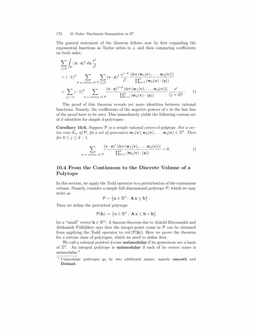
172 10 Euler–Maclaurin Summation in Rd
The general statement of the theorem follows now by first expanding theexponential functions as Taylor series in s, and then comparing coefficientson both sides:∑
j≥0
∫P
(x · z)j dxsj
j!
= (−1)d∑
v a vertex of P
∑j≥0
(v · z)jsj−d
j!|det (w1(v), . . . ,wd(v))|∏d
k=1 (wk(v) · (z))
=∑j≥−d
(−1)d∑
v a vertex of P
(v · z)j+d |det (w1(v), . . . ,wd(v))|∏dk=1 (wk(v) · (z))
sj
(j + d)!. ut
The proof of this theorem reveals yet more identities between rationalfunctions. Namely, the coefficients of the negative powers of s in the last lineof the proof have to be zero. This immediately yields the following curious setof d identities for simple d-polytopes:
Corollary 10.6. Suppose P is a simple rational convex d-polytope. For a ver-tex cone Kv of P, fix a set of generators w1(v),w2(v), . . . ,wd(v) ∈ Zd. Thenfor 0 ≤ j ≤ d− 1, ∑
v a vertex of P
(v · z)j |det (w1(v), . . . ,wd(v))|∏dk=1 (wk(v) · (z))
= 0 . ut
10.4 From the Continuous to the Discrete Volume of aPolytope
In this section, we apply the Todd operator to a perturbation of the continuousvolume. Namely, consider a simple full-dimensional polytope P, which we maywrite as
P ={x ∈ Rd : A x ≤ b
}.
Then we define the perturbed polytope
P(h) :={x ∈ Rd : A x ≤ b + h
}for a “small” vector h ∈ Rm. A famous theorem due to Askold Khovanskiı andAleksandr Pukhlikov says that the integer-point count in P can be obtainedfrom applying the Todd operator to vol (P(h)). Here we prove the theoremfor a certain class of polytopes, which we need to define first.
We call a rational pointed d-cone unimodular if its generators are a basisof Zd. An integral polytope is unimodular if each of its vertex cones isunimodular.1
1 Unimodular polytopes go by two additional names, namely smooth andDelzant.

10.4 From the Continuous to the Discrete Volume of a Polytope 173
Theorem 10.7 (Khovanskiı–Pukhlikov theorem). For a unimodular d-polytope P,
#(P ∩ Zd
)= Toddh vol (P(h))|h=0 .
More generally,
σP(exp z) = Toddh
∫P(h)
exp(x · z) dx
∣∣∣∣∣h=0
.
Proof. We use Theorem 10.4, the continuous version of Brion’s theorem; notethat if P is unimodular, then P is automatically simple. For a vertex coneKv of P, denote its generators by w1(v),w2(v), . . . ,wd(v) ∈ Zd. Then The-orem 10.4 states that∫P
exp(x · z) dx = (−1)d∑
v a vertex of P
exp (v · z) |det (w1(v), . . . ,wd(v))|∏dk=1 (wk(v) · z)
= (−1)d∑
v a vertex of P
exp (v · z)∏dk=1 (wk(v) · z)
, (10.8)
where the last identity follows from Exercise 10.3. A similar formula holdsfor P(h), except that we have to account for the shift of the vertices. Thevector h shifts the facet-defining hyperplanes. This shift of the facets inducesa shift of the vertices; let’s say that the vertex v gets moved along each edgedirection wk (the vectors that generate the vertex cone Kv) by hk(v), so thatP(h) has now the vertex v −
∑dk=1 hk(v)wk(v). If h is small enough, P(h)
will still be simple,2 and we can apply Theorem 10.4 to P(h):
∫P(h)
exp(x · z) dx = (−1)d∑
v a vertex of P
exp((
v −∑dk=1 hk(v)wk(v)
)· z)
∏dk=1 (wk(v) · z)
= (−1)d∑
v a vertex of P
exp(v · z−
∑dk=1 hk(v)wk(v) · z
)∏dk=1 (wk(v) · z)
= (−1)d∑
v a vertex of P
exp(v · z)∏dk=1 exp (−hk(v)wk(v) · z)∏dk=1 (wk(v) · z)
.
Strictly speaking, this formula holds only for h ∈ Qm, so that the verticesof P(h) are rational. Since we will eventually set h = 0, this is a harmlessrestriction. Now we apply the Todd operator:
2 The cautious reader may consult [193, p. 66] to confirm this fact.
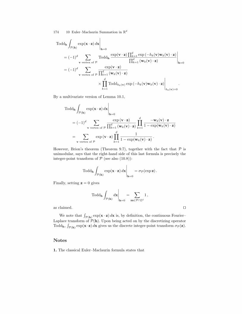
174 10 Euler–Maclaurin Summation in Rd
Toddh
∫P(h)
exp(x · z) dx
∣∣∣∣∣h=0
= (−1)d∑
v vertex of P
Toddhexp(v · z)
∏dk=1 exp (−hk(v)wk(v) · z)∏dk=1 (wk(v) · z)
∣∣∣∣∣h=0
= (−1)d∑
v vertex of P
exp(v · z)∏dk=1 (wk(v) · z)
×d∏k=1
Toddhk(v) exp (−hk(v)wk(v) · z)
∣∣∣∣∣hk(v)=0
.
By a multivariate version of Lemma 10.1,
Toddh
∫P(h)
exp(x · z) dx
∣∣∣∣∣h=0
= (−1)d∑
v vertex of P
exp (v · z)∏dk=1 (wk(v) · z)
d∏k=1
−wk(v) · z1− exp(wk(v) · z)
=∑
v vertex of P
exp (v · z)d∏k=1
11− exp(wk(v) · z)
.
However, Brion’s theorem (Theorem 9.7), together with the fact that P isunimodular, says that the right-hand side of this last formula is precisely theinteger-point transform of P (see also (10.8)):
Toddh
∫P(h)
exp(x · z) dx
∣∣∣∣∣h=0
= σP(exp z) .
Finally, setting z = 0 gives
Toddh
∫P(h)
dx
∣∣∣∣∣h=0
=∑
m∈P∩Zd1 ,
as claimed. ut
We note that∫P(h)
exp(x · z) dx is, by definition, the continuous Fourier–Laplace transform of P(h). Upon being acted on by the discretizing operatorToddh,
∫P(h)
exp(x ·z) dx gives us the discrete integer-point transform σP(z).
Notes
1. The classical Euler–Maclaurin formula states that

Exercises 175
n∑k=1
f(k) =∫ n
0
f(x) dx+f(0) + f(n)
2+
p∑m=1
B2m
(2m)!
[f (2m−1)(x)
]n0
+1
(2p+ 1)!
∫ n
0
B2p+1 ({x}) f (2p+1)(x) dx ,
where Bk(x) denotes the kth Bernoulli polynomial. It was discovered indepen-dently by Leonhard Euler and Colin Maclaurin (1698–1746).3 This formulaprovides an explicit error term, whereas Theorem 10.2 provides a summationformula with no error term.
2. The Todd operator was introduced by Friedrich Hirzebruch in the 1950s[100], following a more complicated definition by J. A. Todd [181, 182] sometwenty years earlier. The Khovanskiı–Pukhlikov theorem (Theorem 10.7)can be interpreted as a combinatorial analogue of the algebro-geometricHirzebruch–Riemann–Roch theorem, in which the Todd operator plays aprominent role.
3. Theorem 10.4, the continuous form of Brion’s theorem, was generalized byAlexander Barvinok to any polytope [11]. In fact, [11] contains a certain ex-tension of Brion’s theorem to irrational polytopes as well. The decompositionformula for moments of a polytope in Theorem 10.5 is due to Michel Brionand Michele Vergne [46].
4. Theorem 10.7 was first proved in 1992 by Askold Khovanskiı and Alek-sandr Pukhlikov [108]. The proof we give here is essentially theirs. Their paper[108] also draws parallels between toric varieties and lattice polytopes. Subse-quently, many attempts to provide formulas for Ehrhart quasipolynomials—some based on Theorem 10.7—have provided fertile ground for deeper con-nections and future work; a long but by no means complete list of referencesis [9, 33, 46, 55, 60, 61, 76, 91, 106, 107, 119, 125, 137, 146, 178].
Exercises
10.1. ♣ Show that Toddh h = h+ 12 . More generally, prove that Toddh hk =
Bk(h+ 1) for k ≥ 1, where Bk(x) denotes the kth Bernoulli polynomial.
10.2. ♣ Prove (10.5): Suppose P is a simple integral d-polytope. For a vertexcone Kv of P, denote its generators by w1(v),w2(v), . . . ,wd(v) ∈ Zd and itsfundamental parallelepiped by Πv. Then∑
m∈P∩( 1nZ)d
exp(m · z) =∑
v a vertex of P
exp(v · z)∑
m∈Πv∩Zd exp(mn · z
)∏dk=1
(1− exp
(wk(v)n · z
)) .
3 For more information about Maclaurin, seehttp://www-groups.dcs.st-and.ac.uk/∼history/Mathematicians/Maclaurin.html.
176 10 Euler–Maclaurin Summation in Rd
10.3. ♣ Given a unimodular cone
K = {v + λ1w1 + λ2w2 + · · ·+ λdwd : λ1, λ2, . . . , λd ≥ 0} ,
where v,w1,w2, . . . ,wd ∈ Zd such that w1,w2, . . . ,wd are a basis for Zd,show that
σK(z) =zv∏d
k=1 (1− zwk)
and |det (w1, . . . ,wd)| = 1.
10.4. ♣ Prove (10.7). That is, for the simplicial cone
K =
{v +
d∑k=1
λkwk : λk ≥ 0
}
with v,w1,w2, . . . ,wd ∈ Qd, show that∫K
exp(x · z) dx = (−1)dexp (v · z) |det (w1(v), . . . ,wd(v))|∏d
k=1 (wk(v) · z).
10.5. Show that in the statement of Theorem 10.4, the expression
|det (w1(v), . . . ,wd(v))|∏dk=1 (wk(v) · z)
remains invariant upon scaling each wk(v) by an independent positive integer.
Open Problems
10.6. Find all differentiable eigenfunctions of the Todd operator.
10.7. Classify all polytopes whose discrete and continuous volumes coincide,that is, LP(1) = volP.
10.8. Which integer polytopes have a triangulation into d-simplices such thateach of the simplices is unimodular?

11
Solid Angles
Everything you’ve learned in school as “obvious” becomes less and less obvious asyou begin to study the universe. For example, there are no solids in the universe.There’s not even a suggestion of a solid. There are no absolute continuums. Thereare no surfaces. There are no straight lines.
Buckminster Fuller (1895–1983)
The natural generalization of a two-dimensional angle to higher dimensions iscalled a solid angle. Given a pointed cone K ⊂ Rd, the solid angle at its apexis the proportion of space that the cone K occupies. In slightly different words,if we pick a point x ∈ Rd “at random,” then the probability that x ∈ K isprecisely the solid angle at the apex of K. Yet another view of solid angles isthat they are in fact volumes of spherical polytopes: the region of intersectionof a cone with a sphere. There is a theory here that parallels the Ehrharttheory of Chapters 3 and 4, but which has some genuinely new ideas.
11.1 A New Discrete Volume Using Solid Angles
Suppose P ⊂ Rd is a convex rational d-polyhedron. The solid angle ωP(x)of a point x (with respect to P) is a real number equal to the proportion of asmall ball centered at x that is contained in P. That is, we let Bε(x) denotethe ball of radius ε centered at x and define
ωP(x) :=vol (Bε(x) ∩ P)
volBε(x)
for all positive ε sufficiently small. We note that when x /∈ P, ωP(x) = 0;when x ∈ P◦, ωP(x) = 1; when x ∈ ∂P, 0 < ωP(x) < 1. The solid angleof a face F of P is defined by picking any point x in the relative interior F◦and setting ωP(F) = ωP(x).
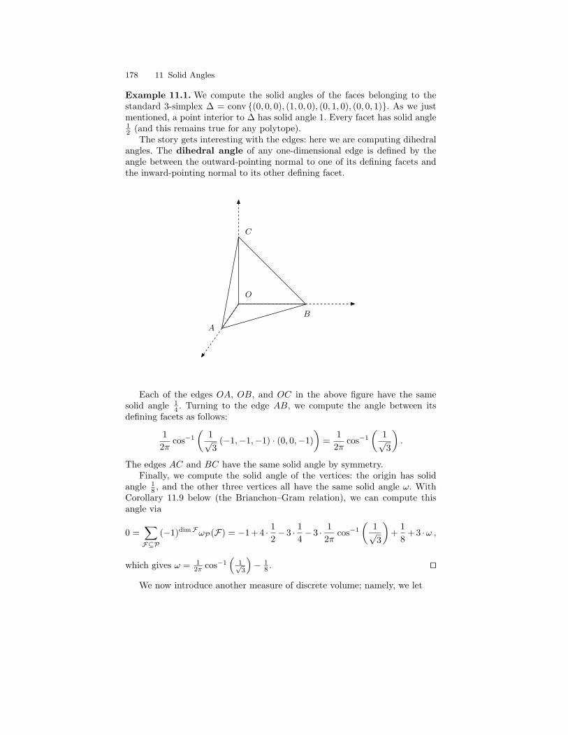
178 11 Solid Angles
Example 11.1. We compute the solid angles of the faces belonging to thestandard 3-simplex ∆ = conv {(0, 0, 0), (1, 0, 0), (0, 1, 0), (0, 0, 1)}. As we justmentioned, a point interior to ∆ has solid angle 1. Every facet has solid angle12 (and this remains true for any polytope).
The story gets interesting with the edges: here we are computing dihedralangles. The dihedral angle of any one-dimensional edge is defined by theangle between the outward-pointing normal to one of its defining facets andthe inward-pointing normal to its other defining facet.
B
C
A
O
Each of the edges OA, OB, and OC in the above figure have the samesolid angle 1
4 . Turning to the edge AB, we compute the angle between itsdefining facets as follows:
12π
cos−1
(1√3
(−1,−1,−1) · (0, 0,−1))
=1
2πcos−1
(1√3
).
The edges AC and BC have the same solid angle by symmetry.Finally, we compute the solid angle of the vertices: the origin has solid
angle 18 , and the other three vertices all have the same solid angle ω. With
Corollary 11.9 below (the Brianchon–Gram relation), we can compute thisangle via
0 =∑F⊆P
(−1)dimFωP(F) = −1 + 4 · 12−3 · 1
4−3 · 1
2πcos−1
(1√3
)+
18
+ 3 ·ω ,
which gives ω = 12π cos−1
(1√3
)− 1
8 . ut
We now introduce another measure of discrete volume; namely, we let

11.1 A New Discrete Volume Using Solid Angles 179
AP(t) :=∑
m∈tP∩ZdωtP(m) ,
the sum of the solid angles at all integer points in tP; recalling that ωP(x) = 0if x /∈ P, we can also write
AP(t) =∑
m∈ZdωtP(m) .
This new discrete volume measure differs in a substantial way from theEhrhart counting function LP(t). Namely, suppose P is a d-polytope that canbe written as the union of the polytopes P1 and P2 such that dim (P1 ∩ P2) <d, that is, P1 and P2 are glued along a lower-dimensional subset. Then at eachlattice point m ∈ Zd, ωP1(m) + ωP2(m) = ωP(m), and so the function APhas an additive property:
AP(t) = AP1(t) +AP2(t) . (11.1)
In contrast, the Ehrhart counting functions satisfy
LP(t) = LP1(t) + LP2(t)− LP1∩P2(t) .
On the other hand, we can transfer computational effort from the Ehrhartcounting functions to the solid-angle sum and vice versa, with the use of thefollowing lemma.
Lemma 11.2. Let P be a polytope. Then
AP(t) =∑F⊆P
ωP(F)LF◦(t) .
Proof. The dilated polytope tP is the disjoint union of its relative open facestF◦, so that we can write
AP(t) =∑
m∈ZdωtP(m) =
∑F⊆P
∑m∈Zd
ωtP(m) 1tF◦(m) .
But ωtP(m) is constant on each relatively open face tF◦, and we called thisconstant ωP(F), whence
AP(t) =∑F⊆P
ωP(F)∑
m∈Zd1tF◦(m) =
∑F⊆P
ωP(F)LF◦(t) . ut
Thus AP(t) is a polynomial (respectively quasipolynomial) in t for anintegral (respectively rational) polytope P. We claim that Lemma 11.2 is infact useful in practice. To drive the point home, we illustrate this identity bycomputing the solid-angle sum over all integer points of ∆ in Example 11.1.

180 11 Solid Angles
Example 11.3. We continue the solid-angle computation for the 3-simplex∆ = conv {(0, 0, 0), (1, 0, 0), (0, 1, 0), (0, 0, 1)}. We recall from Section 2.3 thatL∆◦ =
(t−1
3
). The facets of ∆ are three standard triangles and one triangle
that appeared in the context of the Frobenius problem. All four facets havethe same interior Ehrhart polynomial
(t−1
2
). A similar phenomenon holds for
the edges of ∆: all six of them have the same interior Ehrhart polynomialt − 1. These polynomials add up, by Lemma 11.2 and Example 11.1, to thesolid-angle sum
A∆(t) =(t− 1
3
)+ 4 · 1
2
(t− 1
2
)+(
3 · 14
+ 3 · 12π
cos−1
(1√3
))(t− 1)
+18
+ 3 ·(
12π
cos−1
(1√3
)− 1
8
)=
16t3 +
(3
2πcos−1
(1√3
)− 5
12
)t .
The magic cancellation of the even terms of this polynomial is not a coinci-dence, as we will discover in Theorem 11.7. The curious reader may noticethat the coefficient of t in this example is not a rational number, in starkcontrast with Ehrhart polynomials. ut
The analogue of Ehrhart’s theorem (Theorem 3.23) in the world of solidangles is as follows.
Theorem 11.4 (Macdonald’s theorem). Suppose P is a rational convexd-polytope. Then AP is a quasipolynomial of degree d whose leading coefficientis volP and whose period divides the denominator of P.
Proof. The denominator of a face F ⊂ P divides the denominator of P, andhence so does the period of LF , by Ehrhart’s theorem (Theorem 3.23). ByLemma 11.2, AP is a quasipolynomial with period dividing the denominatorof P. The leading term of AP equals the leading term of LP◦ , which is volP,by Corollary 3.20 and its extension in Exercise 3.29. ut
11.2 Solid-Angle Generating Functions and aBrion-Type Theorem
By analogy with the integer-point transform of a polyhedron P ⊆ Rd, whichlists all lattice points in P, we form the solid-angle generating function
αP(z) :=∑
m∈P∩ZdωP(m) zm.
Using the same reasoning as in (11.1) for AP , this function satisfies a niceadditivity relation. Namely, if the d-polyhedron P equals P1 ∪ P2, wheredim (P1 ∩ P2) < d, then

11.2 Solid-Angle Generating Functions and a Brion-Type Theorem 181
αP(z) = αP1(z) + αP2(z) . (11.2)
This generating function obeys the following reciprocity relation, which par-allels both the statement and proof of Theorem 4.3:
Theorem 11.5. Suppose K is a rational pointed d-cone with the origin asapex, and v ∈ Rd. Then the solid-angle generating function αv+K(z) of thepointed d-cone v +K is a rational function that satisfies
αv+K
(1z
)= (−1)dα−v+K (z) .
Proof. Because solid angles are additive by (11.2), it suffices to prove this the-orem for simplicial cones. The proof for this case proceeds along the same linesas the proof of Theorem 4.2; the main geometric ingredient is Exercise 4.2.We invite the reader to finish the proof (Exercise 11.5). ut
The analogue of Brion’s theorem in terms of solid angles is as follows.
Theorem 11.6. Suppose P is a rational convex polytope. Then we have thefollowing identity of rational functions:
αP(z) =∑
v a vertex of P
αKv(z) .
Proof. As in the proof of Theorem 9.7, it suffices to prove Theorem 11.6 forsimplices. So let ∆ be a rational simplex. We write ∆ as the disjoint union ofits open faces and use Brion’s theorem for open polytopes (Exercise 9.7) oneach face. That is, if we denote the vertex cone of F at vertex v by Kv(F),then by a monomial version of Lemma 11.2,
α∆(z) =∑F⊆∆
ω∆(F)σF◦(z)
=∑
v a vertex of ∆
ω∆(v) zv +∑F⊆∆
dimF>0
ω∆(F)∑
v a vertex of F
σKv(F)◦(z) ,
where we used Brion’s theorem for open polytopes (Exercise 9.7) in the secondstep. By Exercise 11.6,∑F⊆∆
dimF>0
ω∆(F)∑
v a vertex of F
σKv(F)◦(z) =∑
v a vertex of ∆
∑F⊆Kv
dimF>0
ωKv(F)σF◦(z) ,
and so
α∆(z) =∑
v a vertex of ∆
ω∆(v) zv +∑
v a vertex of ∆
∑F⊆Kv
dimF>0
ωKv(F)σF◦(z)
=∑
v a vertex of ∆
∑F⊆Kv
ωKv(F)σF◦(z)
=∑
v a vertex of ∆
αKv(z) . ut
182 11 Solid Angles
11.3 Solid-Angle Reciprocity and the Brianchon–GramRelations
With the help of Theorems 11.5 and 11.6, we can now prove the solid-angleanalogue of Ehrhart–Macdonald reciprocity (Theorem 4.1):
Theorem 11.7 (Macdonald’s reciprocity theorem). Suppose P is a ra-tional convex polytope. Then the quasipolynomial AP satisfies
AP(−t) = (−1)dimPAP(t) .
Proof. We give the proof for an integral polytope P and invite the reader togeneralize it to the rational case. The solid-angle counting function of P canbe computed through the generating function:
AP(t) = αtP(1, 1, . . . , 1) = limz→1
αtP(z) .
By Theorem 11.6,
AP(t) = limz→1
∑v a vertex of P
αtKv(z) ,
where Kv is the tangent cone of P at the vertex v. We write Kv = v +K(v),where K(v) := Kv − v is a rational cone with the origin as its apex. ThentKv = tv + K(v) because a cone whose apex is the origin does not changeunder dilation. Hence we obtain, with the help of Exercise 11.4,
AP(t) = limz→1
∑v a vertex of P
αtv+K(v)(z) = limz→1
∑v a vertex of P
ztvαK(v)(z) .
The rational functions αK(v)(z) on the right-hand side do not depend on t. Ifwe think of the sum over all vertices as one big rational function, to which weapply L’Hopital’s rule to compute the limit as z→ 1, this gives an alternativeproof that AP(t) is a polynomial, in line with our proof for the polynomialityof LP(t) in Section 9.4. At the same time, this means we can view the identity
AP(t) = limz→1
∑v a vertex of P
ztvαK(v)(z)
in a purely algebraic fashion: on the left-hand side we have a polynomial thatmakes sense for any complex t, and on the right-hand side we have a rationalfunction of z, whose limit we compute, for example, by L’Hopital’s rule. Sothe right-hand side, as a function of t, makes sense for any integer t. Hencewe have the algebraic relation, for integral t,
AP(−t) = limz→1
∑v a vertex of P
z−tvαK(v)(z) .

11.3 Solid-Angle Reciprocity and the Brianchon–Gram Relations 183
But now by Theorem 11.5, αK(v)(z) = (−1)dαK(v)
(1z
), and so
AP(−t) = limz→1
∑v a vertex of P
z−tv(−1)d αK(v)
(1z
)
= (−1)d limz→1
∑v a vertex of P
(1z
)tvαK(v)
(1z
)= (−1)d lim
z→1
∑v a vertex of P
αtv+K(v)
(1z
)= (−1)d lim
z→1αtP
(1z
)= (−1)dAP(t) .
In the third step we used Exercise 11.4 again.This proves Theorem 11.7 for integral polytopes. The proof for rational
polytopes follows along the same lines; one deals with rational vertices in thesame manner as in our second proof of Ehrhart’s theorem in Section 9.4. Weinvite the reader to finish the details in Exercise 11.7. ut
We remark that throughout the proof, we cannot simply take the limitinside the finite sum over the vertices of P, since z = 1 is a pole of each rationalfunction αK(v). It is precisely the magic of Brion’s theorem that makes thesepoles cancel each other, to yield AP(t).
If P is an integral polytope, then AP is a polynomial, and Theorem 11.7tells us that AP is always even or odd:
AP(t) = cd td + cd−2t
d−2 + · · ·+ c0 .
We can say more.
Theorem 11.8. Suppose P is a rational convex polytope. Then AP(0) = 0.
This is a meaningful zero. We note that the constant term of AP is given by
AP(0) =∑F⊆P
ωP(F)LF◦(0) =∑F⊆P
ωP(F) (−1)dimF ,
by Lemma 11.2 and Ehrhart–Macdonald reciprocity (Theorem 4.1). HenceTheorem 11.8 implies a classical and useful geometric identity:
Corollary 11.9 (Brianchon–Gram relation). For a rational convex poly-tope P, ∑
F⊆P
(−1)dimFωP(F) = 0 .

184 11 Solid Angles
Example 11.10. Consider a triangle T in R2 with vertices v1,v2,v3 andedges E1, E2, E3. The Brianchon–Gram relation tells us that for this triangle,
ωT (v1) + ωT (v2) + ωT (v3)− (ωT (E1) + ωT (E2) + ωT (E3)) + ωT (T ) = 0 .
Since the solid angles of the edges are all 12 and ωT (T ) = 1, we recover
our friendly high-school identity “the sum of the angles in a triangle is 180degrees”:
ωT (v1) + ωT (v2) + ωT (v3) =12.
Thus the Brianchon–Gram relation is the extension of this well-known fact toany dimension and any convex polytope. ut
Proof of Theorem 11.8. It suffices to prove A∆(0) = 0 for a rational simplex∆, since solid angles of a triangulation simply add, by (11.1). Theorem 11.7gives A∆(0) = 0 if dim ∆ is odd.
So now suppose ∆ is a rational d-simplex, where d is even, with verticesv1,v2, . . . ,vd+1. Let P(n) be the (d+ 1)-dimensional pyramid that we obtainby taking the convex hull of (v1, 0) , (v2, 0) , . . . , (vd+1, 0), and (0, 0, . . . , 0, n),where n is a positive integer (see Figure 11.1). Note that, since d+ 1 is odd,
x1
x2
x3
n
Fig. 11.1. The pyramid P(n) for a triangle ∆.
AP(n)(0) =∑
F(n)⊆P(n)
(−1)dimF(n)ωP(n)(F(n)) = 0 .
We will conclude from this identity that∑F⊆∆(−1)dimFω∆(F) = 0, which
implies that A∆(0) = 0. To this end, we consider two types of faces of P(n):
(a) those that are also faces of ∆, and
11.3 Solid-Angle Reciprocity and the Brianchon–Gram Relations 185
(b) those that are not contained in ∆.
We start with the latter: Aside from the vertex (0, 0, . . . , 0, n), every face F(n)of P(n) that is not a face of ∆ is the pyramid over a face G of ∆; let’s denotethis pyramid by Pyr (G, n). Further, as n grows, the solid angle of Pyr (G, n)(in P(n)) approaches the solid angle of G (in ∆):
limn→∞
ωP(n) (Pyr (G, n)) = ω∆ (G) ,
since we’re forming ∆×[0,∞) in the limit. On the other hand, a face F(n) = Gof P(n) that is also a face of ∆ obeys the following limit behavior:
limn→∞
ωP(n) (F(n)) =12ω∆ (G) .
The only face of P(n) that we still have to account for is the vertex v :=(0, 0, . . . , 0, n). Hence
0 =∑
F(n)⊆P(n)
(−1)dimF(n)ωP(n)(F(n))
= ωP(n)(v) +∑G⊆∆
(−1)dimG+1ωP(n) (Pyr (G, n))
+∑G⊆∆
(−1)dimGωP(n) (G) .
Now we take the limit as n→∞ on both sides; note that limn→∞ ωP(n)(v) =0, so that we obtain
0 =∑G⊆∆
(−1)dimG+1ω∆ (G) +∑G⊆∆
(−1)dimG 12ω∆ (G)
=12
∑G⊆∆
(−1)dimG+1ω∆ (G) ,
and soA∆(0) =
∑G⊆∆
(−1)dimGω∆(G) = 0 . ut
The combination of Theorems 11.7 and 11.8 implies that summing solidangles in a polygon is equivalent to computing its area:
Corollary 11.11. Suppose P is a 2-dimensional integral polytope with areaA. Then AP(t) = A t2.

186 11 Solid Angles
11.4 The Generating Function of Macdonald’sSolid-Angle Polynomials
We conclude this chapter with the study of the solid-angle analogue of Ehrhartseries. Given an integral polytope P, we define the solid-angle series of P asthe generating function of the solid-angle polynomial, encoding the solid-anglesum over all dilates of P simultaneously:
SolidP(z) :=∑t≥0
AP(t) zt.
The following theorem is the solid-angle analogue to Theorems 3.12 and 4.4,with the added bonus that we get the palindromy of the numerator of SolidPfor free.
Theorem 11.12. Suppose P is an integral d-polytope. Then SolidP is a ra-tional function of the form
SolidP(z) =adz
d + ad−1zd−1 + · · ·+ a1z
(1− z)d+1.
Furthermore, we have the identity
SolidP
(1z
)= (−1)d+1 SolidP(z)
or, equivalently, ak = ad+1−k for 1 ≤ k ≤ d2 .
Proof. The form of the rational function SolidP follows by Lemma 3.9 fromthe fact that AP is a polynomial. The palindromy of a1, a2, . . . , ad is equivalentto the relation
SolidP
(1z
)= (−1)d+1 SolidP(z) ,
which, in turn, follows from Theorem 11.7:
SolidP(z) =∑t≥0
AP(t) zt =∑t≥0
(−1)dAP(−t) zt = (−1)d∑t≤0
AP(t) z−t.
Now we use Exercise 4.6:
(−1)d∑t≤0
AP(t) z−t = (−1)d+1∑t≥1
AP(t) z−t = (−1)d+1 SolidP
(1z
).
In the last step we used the fact that AP(0) = 0 (Theorem 11.8). ut
Exercises 187
Notes
1. I. G. Macdonald inaugurated the systematic study of solid-angle sums inintegral polytopes. The fundamental Theorems 11.4, 11.7, and 11.8 can befound in his 1971 paper [123]. The proof of Theorem 11.7 we give here follows[26].
2. The Brianchon–Gram relation (Corollary 11.9) is the solid-angle analogueof the Euler relation for face numbers (Theorem 5.2). The 2-dimensional casediscussed in Example 11.10 is ancient; it was most certainly known to Euclid.The 3-dimensional case of Corollary 11.9 was discovered by Charles JulienBrianchon in 1837 and—as far as we know—was independently reproved byJørgen Gram in 1874 [88]. It is not clear who first proved the general d-dimensional case of Corollary 11.9. The oldest proofs we could find were fromthe 1960s, by Branko Grunbaum [90], Micha A. Perles, and Geoffrey C. Shep-hard [142, 162].
3. Theorem 11.5 is a particular case of a reciprocity relation for simple lattice-invariant valuations due to Peter McMullen [128], who also proved a parallelextension of Ehrhart–Macdonald reciprocity to general lattice-invariant val-uations. There is a current resurgence of activity on solid angles; see, forexample, [52].
Exercises
11.1. Compute AP(t), where P is the regular tetrahedron with vertices(0, 0, 0), (1, 1, 0), (1, 0, 1), and (0, 1, 1) (see Exercise 2.13).
11.2. Compute AP(t), where P is the rational triangle with vertices (0, 0),(12 ,
12
), and (1, 0).
11.3. For a simplex ∆, let S(∆) denote the sum of the solid angles at thevertices of ∆.
(a) Prove that S(∆) ≤ 12 .
(b) Construct a sequence ∆n of simplices in a fixed dimension, such thatlimn→∞ S(∆n) = 1
2 .
11.4. ♣ Let K be a rational d-cone and let m ∈ Zd. By analogy with Exer-cise 3.5, show that αm+K(z) = zmαK(z).
11.5. ♣ Complete the proof of Theorem 11.5: For a rational pointed d-coneK, αK(z) is a rational function that satisfies
αK
(1z
)= (−1)dαK (z) .

188 11 Solid Angles
11.6. ♣ Suppose ∆ is a rational simplex. Prove that∑F⊆∆
dimF>0
ω∆(F)∑
v a vertex of F
σKv(F)◦(z) =∑
v a vertex of ∆
∑F⊆Kv
dimF>0
ωKv(F)σF◦(z) .
11.7. ♣ Provide the details of the proof of Theorem 11.7 for rational poly-topes: Prove that if P is a rational convex polytope, then the quasipolynomialAP satisfies
AP(−t) = (−1)dimPAP(t) .
11.8. Recall from Exercise 3.1 that to any permutation π ∈ Sd on d elementswe can associate the simplex
∆π := conv{0, eπ(1), eπ(1) + eπ(2), . . . , eπ(1) + eπ(2) + · · ·+ eπ(d)
}.
Prove that for all π ∈ Sn, A∆π(t) = 1
d! td.
11.9. Give a direct proof of Corollary 11.11, e.g., using Pick’s theorem (The-orem 2.8).
11.10. State and prove the analogue of Theorem 11.12 for rational polytopes.
Open Problems
11.11. Study the roots of solid-angle polynomials.
11.12. Classify all polytopes that have only rational solid angles at their ver-tices.
11.13. Which integral polytopes P have solid-angle polynomials AP(t) ∈Q[t]? That is, for which integral polytopes P are all the coefficients of AP(t)rational?
12
A Discrete Version of Green’s Theorem UsingElliptic Functions
The shortest route between two truths in the real domain passes through the complexdomain.
Jacques Salomon Hadamard (1865–1963)
We now allow ourselves the luxury of using basic complex analysis. In par-ticular, we assume that the reader is familiar with contour integration andthe residue theorem. We may view the residue theorem as yet another re-sult that intimately connects the continuous and the discrete: it transforms acontinuous integral into a discrete sum of residues.
Using the Weierstraß ℘ and ζ functions, we show here that Pick’s theoremis a discrete version of Green’s theorem in the plane. As a bonus, we alsoobtain an integral formula (Theorem 12.5 below) for the discrepancy betweenthe area enclosed by a general curve C and the number of integer pointscontained in C.
12.1 The Residue Theorem
We begin this chapter by reviewing a few concepts from complex analysis.Suppose the complex-valued function f has an isolated singularity w ∈ G;that is, there is an open set G ⊂ C such that f is analytic on G \ {w}. Thenf can be expressed locally by the Laurent series
f(z) =∑n∈Z
cn (z − w)n ,
valid for all z ∈ G; here cn ∈ C. The coefficient c−1 is called the residue of fat w; we will denote it by Res(z = w). The reason to give c−1 a special namecan be found in the following theorem. We call a function meromorphic ifit is analytic in C with the exception of isolated poles.

190 12 A Discrete Version of Green’s Theorem Using Elliptic Functions
Theorem 12.1 (Residue theorem). Suppose f is meromorphic and C isa positively oriented, piecewise differentiable, simple, closed curve that doesnot pass through any pole of f . Then∫
C
f = 2πi∑w
Res(z = w) ,
where the sum is taken over all singularities w inside C. ut
If f is a rational function, Theorem 12.1 gives the same result as thepartial fraction expansion of f . We illustrate this philosophy by returning tothe elementary beginnings of Chapter 1.
Example 12.2. Recall our constant-term identity for the restricted partitionfunction for A = {a1, a2, . . . , ad} in Chapter 1:
pA(n) = const(
1(1− za1) (1− za2) · · · (1− zad) zn
).
Computing the constant term of the Laurent series of 1(1−za1 )···(1−zad )zn ex-
panded about z = 0 is, naturally, equivalent to “shifting” this function by oneexponent and computing the residue at z = 0 of the function
f(z) :=1
(1− za1) (1− za2) · · · (1− zad) zn+1.
Now let Cr be a positively oriented circle of radius r > 1, centered at theorigin. The residue Res(z = 0) = pA(n) is one of the residues that are pickedup by the integral
12πi
∫Cr
f = Res(z = 0) +∑w
Res(z = w) ,
where the sum is over all nonzero poles w of f that lie inside Cr. Thesepoles are at the ath
1 , ath2 , . . . , a
thd roots of unity. Moreover, with the help of
Exercise 12.1 we can show that
0 = limr→∞
12πi
∫Cr
f
= limr→∞
(Res(z = 0) +
∑w
Res(z = w)
)= Res(z = 0) +
∑w
Res(z = w) ,
where the sum extends over all ath1 , a
th2 , . . . , a
thd roots of unity. In other words,
pA(n) = Res(z = 0) = −∑w
Res(z = w) .
12.2 The Weierstraß ℘ and ζ Functions 191
To obtain the restricted partition function pA, it remains to compute theresidues at the roots of unity, and we invite the reader to realize that thiscomputation is equivalent to the partial fraction expansion of Chapter 1 (Ex-ercise 12.2). ut
Analogous residue computations could replace any of the constant-termcalculations that we performed in the earlier chapters.
12.2 The Weierstraß ℘ and ζ Functions
The main character in our play is the Weierstraß ζ-function, defined by
ζ(z) =1z
+∑
(m,n)∈Z2\(0,0)
(1
z − (m+ ni)+
1m+ ni
+z
(m+ ni)2
). (12.1)
This infinite sum converges uniformly on compact subsets of the lattice-punctured plane C\Z2 (Exercise 12.4), and hence forms a meromorphic func-tion of z.
The Weierstraß ζ-function possesses the following salient properties, whichfollow immediately from (12.1):
(1) ζ has a simple pole at every integer point m+ni and is analytic elsewhere.(2) The residue of ζ at each integer point m+ ni equals 1.
We can easily check (Exercise 12.5) that
℘(z) := −ζ ′(z) =1z2
+∑
(m,n)∈Z2\(0,0)
(1
(z − (m+ ni))2 −1
(m+ ni)2
),
(12.2)the Weierstraß ℘-function. The ℘-function has a pole of order 2 at eachinteger point m+ni and is analytic elsewhere, but has residue equal to zero ateach integer point m+ni. However, ℘ possesses a very pleasant property thatζ does not: ℘ is doubly periodic on C. We may state this more concretely:
Lemma 12.3. ℘(z + 1) = ℘(z + i) = ℘(z) .
Proof. We first invite the reader to prove the following two properties of ℘′
(Exercises 12.6 and 12.7):
℘′ (z + 1) = ℘′(z) , (12.3)∫ z1
z0
℘′ (z) dz is path independent. (12.4)
By (12.3),d
dz(℘ (z + 1)− ℘(z)) = ℘′ (z + 1)− ℘′(z) = 0 ,

192 12 A Discrete Version of Green’s Theorem Using Elliptic Functions
so ℘ (z + 1)− ℘(z) = c for some constant c. On the other hand, ℘ is an evenfunction (Exercise 12.8), and so z = − 1
2 gives us
c = ℘(
12
)− ℘
(− 1
2
)= 0 .
This shows that ℘ (z + 1) = ℘(z) for all z ∈ C\Z2. An analogous proof, whichwe invite the reader to construct in Exercise 12.9, shows that ℘ (z + i) = ℘(z).
ut
Lemma 12.3 implies that ℘(z + m + ni) = ℘(z) for all m,n ∈ Z. Thefollowing lemma shows that the Weierstraß ζ-function is only a conjugate-analytic term away from being doubly periodic.
Lemma 12.4. There is a constant α such that the function ζ(z)+αz is doublyperiodic with periods 1 and i.
Proof. We begin with w = m+ ni:
ζ (z +m+ ni)− ζ(z) = −∫ m+ni
w=0
℘ (z + w) dw , (12.5)
by definition of ℘(z) = −ζ ′(z). To make sure that (12.5) makes sense, weshould also check that the definite integral in (12.5) is path independent (Ex-ercise 12.10).
Due to the double periodicity of ℘,∫ m+ni
w=0
℘ (z + w) dw = m
∫ 1
0
℘ (z + t) dt+ ni
∫ 1
0
℘ (z + it) dt
= mα(z) + niβ(z) ,
where
α(z) :=∫ 1
0
℘ (z + t) dt and β(z) :=∫ 1
0
℘ (z + it) dt .
Now we observe that α (z + x0) = α(z) for any x0 ∈ R, so that α (x+ iy)depends only on y. Similarly, β (x+ iy) depends only on x. But
ζ (z +m+ in)− ζ(z) = − (mα(y) + inβ(x))
must be analytic for all z ∈ C \ Z2. If we now set m = 0, we conclude thatβ(x) must be analytic in C \ Z2, so that β(x) must be a constant by theCauchy–Riemann equations for analytic functions. Similarly, setting n = 0implies that α(y) is constant. Thus
ζ (z +m+ in)− ζ(z) = − (mα+ inβ)
with constants α and β. Going back to the Weierstraß ℘-function, we canintegrate the identity (Exercise 12.11)
12.3 A Contour-Integral Extension of Pick’s Theorem 193
℘(iz) = −℘(z) (12.6)
to obtain the relationship β = −α, since
β =∫ 1
0
℘ (z + it) dt =∫ 1
0
℘ (it) dt = −∫ 1
0
℘ (t) dt = −α .
To summarize, we have
ζ (z +m+ in)− ζ(z) = −mα+ inα = −α(z +m+ in− z
),
so that ζ(z) + αz is doubly periodic. ut
12.3 A Contour-Integral Extension of Pick’s Theorem
For the remainder of this chapter, let C be any piecewise-differentiable, simple,closed curve in the plane, with a counterclockwise parametrization. We let Ddenote the region that C contains in its interior.
Theorem 12.5. Let C avoid any integer point, that is, C ∩ Z2 = ∅. Let Idenote the number of integer points interior to C, and A the area of the regionD enclosed by the curve C. Then
12πi
∫C
(ζ(z)− πz) dz = I −A .
Proof. We have∫C
(ζ(z) + αz) dz =∫C
ζ(z) dz + α
∫C
(x− iy) (dx+ idy) ,
where α is as in Lemma 12.4. By Theorem 12.1,∫Cζ(z) dz is equal to the sum
of the residues of ζ at all of its interior poles. There are I such poles, and eachpole of ζ has residue 1. Thus
12πi
∫C
ζ(z) dz = I . (12.7)
On the other hand, Green’s theorem tells us that∫C
(x− iy) (dx+ idy) =∫C
(x− iy) dx+ (y + ix) dy
=∫D
∂
∂x(y + ix)− ∂
∂y(x− iy)
=∫ ∫
D
2i
= 2iA .
194 12 A Discrete Version of Green’s Theorem Using Elliptic Functions
Going back to (12.7), we get∫C
(ζ(z) + αz) dz = 2πiI + α (2iA) . (12.8)
We only have to show that α = −π. Consider the particular curve C that isa square path, centered at the origin, traversing the origin counterclockwise,and bounding a square of area 1. Thus I = 1 for this path. Since ζ(z) + αzis doubly periodic by Lemma 12.4, the integral in (12.8) vanishes. We canconclude that
0 = 2πi · 1 + α (2i · 1) ,
so that α = −π. ut
Notice that Theorem 12.5 has given us information about the Weierstraßζ-function, namely that α = −π.
This chapter offers a detour into an infinite landscape of discrete resultsthat meet their continuous counterparts. Equipped with the modest toolsoffered in this book, we hope we have motivated the reader to explore thislandscape further. . .
Notes
1. The Weierstraß ℘-function, named after Karl Theodor Wilhelm Weier-straß (1815–1897),1 can be extended to any two-dimensional lattice L ={kw1 + jw2 : k, j ∈ Z} for some w1, w2 ∈ C that are linearly independentover R:
℘L(z) =1z2
+∑
m∈L\{0}
(1
(z −m)2 −1m2
).
The Weierstraß ℘L-function and its derivative ℘′L satisfy a polynomial rela-tionship, namely, (℘′L)2 = 4 (℘L)3 − g2 ℘L − g3 for some constants g2 and g3
that depend on L. This is the beginning of a wonderful friendship betweencomplex analysis and elliptic curves.
2. Theorem 12.5 appeared in [75]. There it is also shown that one can retrievePick’s theorem (Theorem 2.8) from Theorem 12.5.
Exercises
12.1. ♣ Show that for positive integers a1, ad, . . . , ad, n,
1 For more information about Weierstraß, seehttp://www-groups.dcs.st-and.ac.uk/∼history/Mathematicians/Weierstrass.html.
Open Problems 195
limr→∞
∫Cr
1(1− za1) · · · (1− zad) zn+1
= 0 .
This computation shows that the integrand above “has no pole at infinity.”
12.2. ♣ Compute the residues at the nontrivial roots of unity of
f(z) =1
(1− za1) · · · (1− zad) zn+1.
For simplicity, you may assume that a1, a2, . . . , ad are pairwise relativelyprime.
12.3. Give an integral version of Theorem 2.13.
12.4. ♣ Show that
ζ(z) =1z
+∑
(m,n)∈Z2\(0,0)
(1
z − (m+ ni)+
1m+ ni
+z
(m+ ni)2
)
converges absolutely for z belonging to compact subsets of C \ Z2.
12.5. ♣ Prove (12.2), that is,
ζ ′(z) = − 1z2−
∑(m,n)∈Z2\(0,0)
(1
(z − (m+ ni))2 −1
(m+ ni)2
).
12.6. ♣ Prove (12.3), that is, show that ℘′ (z + 1) = ℘′(z).
12.7. ♣ Prove (12.4), that is, show that for any z0, z1 ∈ C \ Z2,∫ z1z0℘′(w) dw
is path independent.
12.8. ♣ Show that ℘ is even, that is, ℘ (−z) = ℘(z).
12.9. ♣ Finish the proof of Lemma 12.3 by showing that ℘ (z + i) = ℘(z).
12.10. ♣ Prove that the integral in (12.5),
ζ (z +m+ ni)− ζ(z) = −∫ w=m+ni
w=0
℘ (z + w) dw ,
is path independent.
12.11. ♣ Prove (12.6), that is, ℘(iz) = −℘(z).
Open Problems
12.12. Can we get even more information about the Weierstraß ℘ and ζ func-tions by using more detailed knowledge of the discrepancy between I and Afor special curves C?
12.13. Find a complex-analytic extension of Theorem 12.5 to higher dimen-sions.

A
Vertex and Hyperplane Descriptions ofPolytopes
Everything should be made as simple as possible, but not simpler.
Albert Einstein
In this appendix, we prove that every polytope has a vertex and a hyperplanedescription. This appendix owes everything to Gunter Ziegler’s beautiful ex-position in [193]; in fact, these pages contain merely a few cherries picked from[193, Lecture 1].
As in Chapter 3, it is easier to move to the world of cones. To be as concreteas possible, let us call K ⊆ Rd an h-cone if
K ={x ∈ Rd : A x ≤ 0
}for some A ∈ Rm×d; in this case K is given as the intersection of m halfspacesdetermined by the rows of A. We use the notation K = hcone(A).
On the other hand, we call K ⊆ Rd a v-cone if
K = {B y : y ≥ 0}
for some B ∈ Rd×n, that is, K is a pointed cone with the column vectors ofB as generators. In this case we use the notation K = vcone(B).
Note that, according to our definitions, any h- or v-cone contains the originin its apex. We will prove that every h-cone is a v-cone and vice versa. Moreprecisely:
Theorem A.1. For every A ∈ Rm×d there exists B ∈ Rd×n (for some n)such that hcone(A) = vcone(B). Conversely, for every B ∈ Rd×n there existsA ∈ Rm×d (for some m) such that vcone(B) = hcone(A).
We will prove the two halves of Theorem A.1 in Sections A.1 and A.2. Fornow, let us record that Theorem A.1 implies our goal, that is, the equivalenceof the vertex and halfspace description of a polytope:

198 Appendix A: Vertex and Hyperplane Descriptions of Polytopes
Corollary A.2. If P is the convex hull of finitely many points in Rd, then Pis the intersection of finitely many half-spaces in Rd. Conversely, if P is givenas the bounded intersection of finitely many half-spaces in Rd, then P is theconvex hull of finitely many points in Rd.
Proof. If P = conv {v1,v2, . . . ,vn} for some v1,v2, . . . ,vn ∈ Rd, then coningover P (as defined in Chapter 3) gives
cone(P) = vcone(
v1 v2 . . . vn1 1 1
).
By Theorem A.1 we can find a matrix (A,b) ∈ Rm×(d+1) such that
cone(P) = hcone(A,b) ={x ∈ Rd+1 : (A,b) x ≤ 0
}.
We recover the polytope P upon setting xd+1 = 1, that is,
P ={x ∈ Rd : Ax ≤ −b
},
which is a hyperplane description of P.These steps can be reversed: Suppose the polytope P is given as
P ={x ∈ Rd : Ax ≤ −b
}for some A ∈ Rm×d and b ∈ Rm. Then P can be obtained from
hcone(A,b) ={x ∈ Rd+1 : (A,b) x ≤ 0
}by setting xd+1 = 1. By Theorem A.1 we can construct a matrix B ∈ R(d+1)×n
such thathcone(A,b) = vcone(B) .
We may normalize the generators of vcone(B), that is, the columns of B, suchthat they all have (d+ 1)st variable equal to one:
B =(
v1 v2 . . . vn1 1 1
).
Since P can be recovered from vcone(B) by setting xd+1 = 1, we concludethat P = conv {v1,v2, . . . ,vn}. ut
A.1 Every h-cone is a v-cone
SupposeK = hcone(A) =
{x ∈ Rd : Ax ≤ 0
}for some A ∈ Rm×d. We introduce an auxiliary m-dimensional variable y andwrite

A.1 Every h-cone is a v-cone 199
K ={(
xy
)∈ Rd+m : A x ≤ y
}∩{(
xy
)∈ Rd+m : y = 0
}. (A.1)
(Strictly speaking, this is K lifted into a d-dimensional subspace of Rd+m.)Our goal in this section is to prove the following two lemmas.
Lemma A.3. The h-cone{(
xy
)∈ Rd+m : A x ≤ y
}is a v-cone.
Lemma A.4. If K ⊆ Rd is a v-cone, then so is K ∩{x ∈ Rd : xk = 0
}, for
any k.
The first half of Theorem A.1 follows with these two lemmas, as we can startwith (A.1) and intersect with one hyperplane yk = 0 at a time.
Proof of Lemma A.3. We start by noting that
K ={(
xy
)∈ Rd+m : A x ≤ y
}={(
xy
)∈ Rd+m : (A,−I)
(xy
)≤ 0
}is an h-cone; here I represents an m ×m identity matrix. Let us denote thekth unit vector by ek. Then we can decompose(
xy
)=
d∑j=1
xj
(ej
A ej
)+
m∑k=1
(yk − (A x)k)(
0ek
)
=d∑j=1
|xj | sign (xj)(
ejA ej
)+
m∑k=1
(yk − (A x)k)(
0ek
).
Note that if(xy
)∈ K then yk− (A x)k ≥ 0 for all k, and so
(xy
)can be written
as a nonnegative linear combination of the vectors sign (xj)(
ejAej
), 1 ≤ j ≤ d,
and(
0ek
), 1 ≤ k ≤ m. But this means that K is a v-cone. ut
Proof of Lemma A.4. Suppose K = vcone(B), where B has the column vec-tors b1,b2, . . . ,bn ∈ Rd; that is, b1,b2, . . . ,bn are the generators of K. Fixk ≤ d and construct a new matrix Bk whose column vectors are all bj forwhich bjk = 0, and the combinations bikbj − bjkbi whenever bik > 0 andbjk < 0. We claim that
K ∩{x ∈ Rd : xk = 0
}= vcone (Bk) .
Every x ∈ vcone (Bk) satisfies xk = 0 by construction of Bk, and sovcone (Bk) ⊆ K∩
{x ∈ Rd : xk = 0
}follows immediately. We need to do some
more work to prove the reverse containment.

200 Appendix A: Vertex and Hyperplane Descriptions of Polytopes
Suppose x ∈ K∩{x ∈ Rd : xk = 0
}, that is, x = λ1b1 +λ2b2 + · · ·+λnbn
for some λ1, λ2, . . . , λn ≥ 0 and xk = λ1b1k + λ2b2k + · · · + λnbnk = 0. Thisallows us to define
Λ =∑
i: bik>0
λibik = −∑
j: bjk<0
λjbjk .
Note that Λ ≥ 0. Now consider the decomposition
x =∑
j: bjk=0
λjbj +∑
i: bik>0
λibi +∑
j: bjk<0
λjbj . (A.2)
If Λ = 0 then λibik = 0 for all i such that bik > 0, and so λi = 0 for these i.Similarly, λj = 0 for all j such that bjk < 0. Thus we conclude from Λ = 0that
x =∑
j: bjk=0
λjbj ∈ vcone (Bk) .
Now assume Λ > 0. Then we can expand the decomposition (A.2) into
x =∑
j: bjk=0
λjbj +1Λ
− ∑j: bjk<0
λjbjk
( ∑i: bik>0
λibi
)
+1Λ
( ∑i: bik>0
λibik
) ∑j: bjk<0
λjbj
=
∑j: bjk=0
λjbj +1Λ
∑i: bik>0j: bjk<0
λiλj (bikbj − bjkbi) ,
which is by construction in vcone (Bk). ut
A.2 Every v-cone is an h-cone
SupposeK = vcone(B) = {B y : y ≥ 0}
for some B ∈ Rd×n. Then K is the projection of{(xy
)∈ Rd+n : y ≥ 0, x = B y
}(A.3)
to the subspace{(
xy
)∈ Rd+n : y = 0
}. The constraints for (A.3) can be writ-
ten as
y ≥ 0 and (I,−B)(
xy
)= 0 .
Thus the set (A.3) is an h-cone, for which we can project one component ofy at a time to obtain K. This means that it suffices to prove the followinglemma to finish the second half of Theorem A.1.
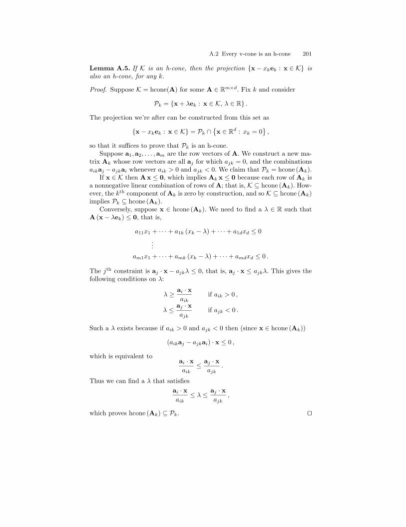
A.2 Every v-cone is an h-cone 201
Lemma A.5. If K is an h-cone, then the projection {x− xkek : x ∈ K} isalso an h-cone, for any k.
Proof. Suppose K = hcone(A) for some A ∈ Rm×d. Fix k and consider
Pk = {x + λek : x ∈ K, λ ∈ R} .
The projection we’re after can be constructed from this set as
{x− xkek : x ∈ K} = Pk ∩{x ∈ Rd : xk = 0
},
so that it suffices to prove that Pk is an h-cone.Suppose a1,a2, . . . ,am are the row vectors of A. We construct a new ma-
trix Ak whose row vectors are all aj for which ajk = 0, and the combinationsaikaj − ajkai whenever aik > 0 and ajk < 0. We claim that Pk = hcone (Ak).
If x ∈ K then A x ≤ 0, which implies Ak x ≤ 0 because each row of Ak isa nonnegative linear combination of rows of A; that is, K ⊆ hcone (Ak). How-ever, the kth component of Ak is zero by construction, and so K ⊆ hcone (Ak)implies Pk ⊆ hcone (Ak).
Conversely, suppose x ∈ hcone (Ak). We need to find a λ ∈ R such thatA (x− λek) ≤ 0, that is,
a11x1 + · · ·+ a1k (xk − λ) + · · ·+ a1dxd ≤ 0...
am1x1 + · · ·+ amk (xk − λ) + · · ·+ amdxd ≤ 0 .
The jth constraint is aj · x − ajkλ ≤ 0, that is, aj · x ≤ ajkλ. This gives thefollowing conditions on λ:
λ ≥ ai · xaik
if aik > 0 ,
λ ≤ aj · xajk
if ajk < 0 .
Such a λ exists because if aik > 0 and ajk < 0 then (since x ∈ hcone (Ak))
(aikaj − ajkai) · x ≤ 0 ,
which is equivalent toai · xaik
≤ aj · xajk
.
Thus we can find a λ that satisfiesai · xaik
≤ λ ≤ aj · xajk
,
which proves hcone (Ak) ⊆ Pk. ut


B
Triangulations of Polytopes
Obvious is the most dangerous word in mathematics.
Eric Temple Bell
The goal of this appendix is to prove Theorem 3.1. Recall that a triangula-tion of a convex d-polytope P is a finite collection T of d-simplices with thefollowing properties:
• P =⋃
∆∈T∆ .
• For any ∆1,∆2 ∈ T , ∆1 ∩∆2 is a face common to both ∆1 and ∆2.
Theorem 3.1 says that P can be triangulated using no new vertices, that is,there exists a triangulation T such that the vertices of any ∆ ∈ T are verticesof P. In preparation, we first show that a triangulation of a polytope inducesa triangulation on any of its facets in a natural way.
Lemma B.1. Suppose T (P) is a triangulation of the d-polytope P, and F isa facet of P. Then
T (F) := {S ∩ F : S ∈ T (P), dim (S ∩ F) = d− 1}
is a triangulation of F .
Proof. To avoid unnecessary notation, we write⋃T (F) for
⋃∆∈T (F) ∆. We
have to show:
(i) F =⋃T (F) .
(ii) For any ∆1,∆2 ∈ T (F), ∆1 ∩∆2 is a face common to both ∆1 and ∆2.
(i) First,⋃T (F) ⊆ F by definition of T (F). Now we will show that F \⋃
T (F) = ∅, by means of contradiction. Let x ∈ F \⋃T (F). If there is a
neighborhood N of x in F that contains no points of⋃T (F), then N consists

204 Appendix B: Triangulations of Polytopes
only of points contained in some simplices from T (P) that meet F in a set ofdimension less than d− 1, which is impossible since dimN = d− 1 and thereare only finitely many simplices in T (P). Hence any neighborhood of x in Fcontains points in some ∆ ∈ T (F). However,
⋃T (F) is closed, and so such
an x cannot exist. Hence F \⋃T (F) = ∅.
(ii) Given ∆1,∆2 ∈ T (F), there are S1,S2 ∈ T (P) such that
∆1 = S1 ∩ F and ∆2 = S2 ∩ F
and the intersections of both S1 and S2 with F are (d− 1)-dimensional. Now∆1 ∩∆2 = S1 ∩ S2 ∩F , and since S1,S2 ∈ T (P), S1 ∩ S2 is a face of both S1
and S2. That is, there are hyperplanes H1 and H2 in Rd such that
S1 ∩ S2 = S1 ∩H1 and S1 ∩ S2 = S2 ∩H2 .
The (d− 1)-hyperplanes H1, H2 in Rd induce the (d− 2)-hyperplanes
h1 := H1 ∩ spanF and h2 := H2 ∩ spanF
in spanF . We claim that h1 ∩∆1 = ∆1 ∩∆2 = h2 ∩∆2, that is, ∆1 ∩∆2 is aface of both ∆1 and ∆2. Indeed,
h1 ∩∆1 = h1 ∩ (S1 ∩ F)= (H1 ∩ spanF) ∩ (S1 ∩ F)= (H1 ∩ S1) ∩ (F ∩ spanF)= (S1 ∩ S2) ∩ F= ∆1 ∩∆2 ,
and a practically identical calculation gives h2 ∩∆2 = ∆1 ∩∆2 . ut
Proof of Theorem 3.1. We use induction on the number of vertices of the d-polytope P. If P has d+ 1 vertices, then P is a simplex, and {P} is a trian-gulation.
For the induction step, suppose we are given a d-polytope P with at leastd+2 vertices. Fix a vertex v of P such that Q, the convex hull of the remainingvertices of P, is still of dimension d. By the induction hypothesis, we cantriangulate Q.
We call a facet F of Q visible from v if for any x ∈ F , the half-open linesegment (x,v] is disjoint from Q. By the Lemma, the triangulation T (Q) ofQ induces the triangulation
T (F) = {∆ ∩ F : ∆ ∈ T (Q), dim (∆ ∩ F) = d− 1}
of a facet F of Q.Let T consist of the convex hulls of v with each (d− 1)-simplex in the tri-
angulations of the visible facets. We claim that T ∪T (Q) forms a triangulationof P. To prove this, we have to show:

Appendix B: Triangulations of Polytopes 205
(i) P =⋃
(T ∪ T (Q)) .(ii) For any ∆1,∆2 ∈ T ∪ T (Q), ∆1 ∩ ∆2 is a face common to both ∆1
and ∆2.
(i) P ⊇⋃
(T ∪ T (Q)) follows by the definitions of T and T (Q). To proveP ⊆
⋃(T ∪ T (Q)), assume x ∈ P is given. If x ∈ Q then x ∈
⋃T (Q). If
x ∈ P \Q, consider the line through v and x. This line meets Q (because P isconvex), so let y ∈ Q be the first point in Q that we meet when traveling alongthe line towards Q. This point y is on a facet of Q that is, by construction,visible from v, and hence x ∈ ∆ for some ∆ ∈ T .
(ii) Given ∆1,∆2 ∈ T ∪ T (Q), there are three cases:
(a) ∆1,∆2 ∈ T (Q);(b) ∆1,∆2 ∈ T ;(c) ∆1 ∈ T,∆2 ∈ T (Q).
In each case we have to show that ∆1 ∩∆2 is a face common to ∆1 and ∆2.
(a) Since T (Q) is a triangulation, ∆1 ∩∆2 is a face of both ∆1 and ∆2.
(b) Given ∆1,∆2 ∈ T , there exist S1, S2 ∈ T (F) such that ∆1 = conv {v, S1}and ∆2 = conv {v, S2}. Since T (F) is a triangulation, S1∩S2 is a face commonto S1 and S2. By convexity, ∆1 ∩∆2 = conv {v, S1 ∩ S2}. Exercise 2.6 showsthat S1 ∩ S2 is a simplex, and that this simplex is the convex hull of someof the common vertices of S1 and S2. But then ∆1 ∩∆2 = conv {v, S1 ∩ S2}is the convex hull of some of the common vertices of ∆1 and ∆2 and hence,again by Exercise 2.6, a face of both ∆1 and ∆2.
(c) Since ∆1 ∈ T , there exists S ∈ T (F) such that ∆1 = conv {v, S}. Byconstruction, ∆1 ∩ Q = S, and S is a face of some ∆ ∈ T (Q). Since T (Q) isa triangulation, ∆ ∩∆2 is a face common to ∆ and ∆2. But then
∆1 ∩∆2 = S ∩∆2 = (S ∩∆) ∩∆2 = S ∩ (∆ ∩∆2)
is an intersection of two faces of ∆ and hence by Exercise 2.6 again a face of∆ and a simplex. The vertices of ∆1 ∩ ∆2 = S ∩ (∆ ∩∆2) form a subset ofthe vertices common to S and ∆2. Since S is a face of ∆1, ∆1 ∩∆2 is a faceof both ∆1 and ∆2, by Exercise 2.6. ut

Hints for ♣ Exercises
Well here’s another clue for you all.
John Lennon & Paul McCartney (“Glass Onion,” The White Album)
Chapter 1
1.1 Set up the partial fraction expansion as
z
1− z − z2=
A
1− 1+√
52 z
+B
1− 1−√
52 z
and clear denominators to compute A and B; one can do so, for example, byspecializing z.
1.2 Multiply out (1 − z)(1 + z + z2 + · · ·+ zn
). For the infinite sum, note
that limk→∞ zk = 0 if |z| < 1.
1.3 Start with the observation that there are bxc + 1 lattice points in theinterval [0, x].
1.4 (i) & (j) Write n = qm + r for some integers q, r such that 0 ≤ r < m.Distinguish the cases r = 0 and r > 0.
1.9 Use the fact that if m and n are relatively prime, given any a ∈ Z thereexists b ∈ Z (which is unique modulo n) such that mb ≡ a (mod n). For thesecond equality of sets, think about the case a = 0.
1.12 First translate the line segment to the origin and explain why this trans-lation leaves the integer-point enumeration invariant. For the case (a, b) =(0, 0), first study the problem under the restriction that gcd (c, d) = 1.
1.17 Given a triangle T with vertices on the integer lattice, consider theparallelogram P formed by two fixed edges of T . Use integral translates of P

208 Hints for ♣ Exercises
to tile the plane R2. Conclude from this tiling that P contains only its verticesas lattice points if and only if the area of P is 1.
1.20 Given an integer b, the Euclidean algorithm asserts the existenceof m1,m2, . . . ,md ∈ Z such that b can be represented as b = m1a1 +m2a2 + · · · + mdad. Convince yourself that we can demand that in this rep-resentation 0 ≤ m2,m3, . . . ,md < a1. Conclude that all integers beyond(a1 − 1) (a2 + a3 + · · ·+ ad) are representable in terms of a1, a2, . . . , ad. (Thisargument can be refined to yield another proof of Theorem 1.2.)
1.21 Use the setup
f(z) =A1
z+A2
z2+ · · ·+ An
zn+
B1
z − 1+
B2
(z − 1)2+a−1∑k=1
Ckz − ξka
+b−1∑j=1
Dj
z − ξjb.
To compute Ck, multiply both sides by(z − ξka
)and calculate the limit as
z → ξka . The coefficients Dj can be computed in a similar fashion.
1.22 Use Exercise 1.9 (with m = b−1) on the left-hand side of the equation.
1.24 Suppose a > b. The integer a+ b certainly has a representation in termsof a and b, namely, 1 · a + 1 · b. Think about how the coefficient of b wouldchange if we changed the coefficient of a.
1.29 Use the partial fraction setup (1.11), multiply both sides by(z − ξka1
),
and take the limit as z → ξka1.
1.31 Convince yourself of the generating-function setup∑n≥1
p◦A(n) zn =(
za1
1− za1
)(za2
1− za2
)· · ·(
zad
1− zad
).
Now use the machinery of Section 1.5.
Chapter 2
2.1 Use Exercise 1.3 for the closed interval. For open intervals, you canuse Exercise 1.4(j) or the d. . . e notation of Exercise 1.4(e). To show thequasipolynomial character, rewrite the greatest-integer function in terms ofthe fractional-part function.
2.2 Write R as a direct product of two intervals and use Exercise 1.3.
2.6 Start by showing that the convex hull of a d-element subset W of V isa face of ∆. This allows you to prove the first statement by induction (usingExercise 2.5). For the converse statement, given a supporting hyperplane Hthat defines the face F of ∆, let W ⊆ V consist of those vertices of ∆ thatare in H. Now prove that any point
Hints for ♣ Exercises 209
x = λ1v1 + λ2v2 + · · ·+ λd+1vd+1
in F has to satisfy λk = 0 for all vk /∈W .
2.7 First show that the linear inequalities and equations describing a rationalpolytope can be chosen with rational coefficients, and then clear denominators.
2.8
(a) Prove that, as rational functions,∑j≥0 j
dzj = (−1)d+1∑j≥0 j
d(
1z
)j .(b) Use the fact that
Pdk=0 A(d,k)zk
(1−z)d+1 = z ddz
(Pd−1k=0 A(d−1,k)zk
(1−z)d
).
(c) Start by proving one of the remarks in the Notes of Chapter 2, namely,that A (d, k) counts the permutations of {1, 2, . . . , d} with k − 1 ascents.
(d) Use the fact that∑dk=0A (d, k) zk = (1− z)d+1
∑j≥0 j
dzj .
2.9 Write 1(1−z)d+1 =
(∑k1≥0 z
k1
)(∑k2≥0 z
k2
)· · ·(∑
kd+1≥0 zkd+1
)and
come up with a combinatorial enumeration scheme to compute the coefficientsof this power series.
2.10 Write(t+kd
)= (t+k)(t+k−1)···(t+k−d+1)
d! and switch t to −t.
2.14 Think about the poles of the function zez−1 and use a theorem from
complex analysis.
2.15 Compute the generating function of Bd(1− x) and rewrite it as ze−xz
1−e−z .
2.16 Show that zez−1 + 1
2z is an even function of z.
2.23 Follow the steps of the proof of Theorem 2.4.
2.24 Extend T to a rectangle whose diagonal is the hypotenuse of T , andconsider the lattice points on this diagonal separately.
2.25 For the area use elementary calculus. For the number of boundarypoints on tP, extend Exercise 1.12 to a set of line segments whose unionforms a simple closed curve.
2.31 Rewrite the inequality as(⌈tad
⌉− 1)e+
(⌈tbd
⌉− 1)f ≤ tr and compare
this with the definition of T .
2.32 To compute C3, multiply both sides of (2.20) by (z − 3)2 and computethe limit as z → 1. The coefficients Aj and Bl can be computed in a similarfashion. To compute C2, first move C3
(z−1)3 in (2.20) to the left-hand side,then multiply by (z − 1)2 and take the limit as z → 1. A similar, even moreelaborate, computation gives C1. (Alternatively, compute the Laurent seriesof the function in (2.20) at z = 1 with a computer algebra system such asMaple or Mathematica.)
2.34 Follow the proof of Theorem 2.10. Use Exercise 2.33 to compute the ad-ditional coefficients in the partial fraction expansion of the generating functioncorresponding to this lattice-point count.
210 Hints for ♣ Exercises
2.36 Start with computing the constant term of
1(1− z1z2) (1− z2
1z2) (1− z1) (1− z2) z3t1 z
2t2
with respect to z2 by treating z1 as a constant and setting up a partial fractionexpansion of this function with respect to z2.
Chapter 3
3.2 Write the simplicial cones as cones over simplices and use Exercise 2.6.
3.4 Write down a typical term of the product
σS (z1, z2, . . . , zm)σT (zm+1, zm+2, . . . , zm+n) .
3.5 Multiply out zmσK(z).
3.6 Write a typical term in σS
(1z1, 1z2, . . . , 1
zd
)= σS
(z−1
1 , z−12 , . . . , z−1
d
).
3.8 Given the polynomial f , split up the generating function on the left-handside according to the terms of f and use (2.2). Conversely, if the polynomialg is given, use (2.6).
3.13 Show that H ∩ Zd is a Z-module. Therefore it has a basis; extend thisbasis to a basis of Zd.
3.14 Start by proving the result for a single hyperplane, for example, byreferring to Exercise 3.13.
3.19 Given f , split up the generating function on the left-hand side accordingto the constituents of f ; then use Exercise 3.8. Conversely, given g and h,multiply both by a polynomial to get the denominator on the right-hand sideinto the form (1− zp)d+1; then use (2.6).
3.20 Start with the setup on page 73, and closely orient yourself along theproof of Theorem 3.8.
3.29 Use Lemma 3.19.
Chapter 4
4.1 Use Exercise 2.1.
4.2 Use the explicit description of Π given by (4.3).
4.3 Consider each simplicial cone Kj separately, and look at the arrangementof its bounding hyperplanes. For each hyperplane, use Exercise 3.13.

Hints for ♣ Exercises 211
4.6 For (a), convince yourself that Q(−t) is also a quasipolynomial. For (b),use (1.3). For (c), differentiate (1.3). For (d), think about one constituent ofthe quasipolynomial at a time.
4.7 In the generating function for LP(t−k), make a change in the summationvariable; then use Theorem 4.4.
4.12 Use the fact that A has only integral entries. For the second part, writedown the explicit hyperplane descriptions of (t+ 1)P◦ and tP.
4.13 Assume that there exist t ∈ Z and a facet hyperplane H of P such thatthere is a lattice point between tH and (t+ 1)H. Translate this lattice pointto a lattice point that violates (4.12).
Chapter 5
5.4 Consider an interval [F ,P] in the face lattice of P: [F ,P] contains allfaces G such that F ⊆ G ⊆ P. Prove that if P is simple, any such interval isisomorphic to a Boolean lattice.
5.5 Use Exercise 2.6 to show that the face lattice of a simplex is isomorphicto a Boolean lattice.
Chapter 6
6.1 Think permutation matrices.
6.3 Show that the rank of (6.5) is 2n− 1.
6.5 Start by showing that all permutation matrices are indeed vertices. Thenuse Exercise 6.4 to show that there are no other vertices.
6.6 Establish a bijection between semimagic squares with line sum t−n andsemimagic squares with positive entries and line sum t.
6.7 Think about the smallest possible line sum if the entries of the squareare positive integers.
6.8 Follow the computation on page 110 that led to the formula for H2.
6.9 Multiply both sides of (6.7) by(w − 1
zk
)and take the limit as w → 1
zk.
6.10 Orient yourself along the computation in (6.10).
6.16 Compute the matrix equivalent to (6.5) for the polytope describing allmagic squares of a given size. Show that this matrix has rank 2n+ 1.
6.18 Orient yourself along the computation on page 110.

212 Hints for ♣ Exercises
Chapter 7
7.2 Use Exercise 7.1.
7.5 Differentiate (1.3).
7.6 Use (1.3).
7.7 Write an arbitrary function on Z with period b in terms of δm(x), 1 ≤m ≤ b.
7.8 Use the definition (7.6) of the inner product and the properties zz = |z|2and (zw) = z · w for complex numbers z and w.
7.14 Use the definition (7.4) and simplify the fractional-part function in thesum on the right-hand side.
7.22 Use the definition of F.
Chapter 8
8.5 Use Exercise 1.9.
8.7 Use the methods outlined in the hints for Exercises 1.21 and 2.32 tocompute the partial fraction coefficients for z = 1 in (8.3).
8.9 Multiply out all the terms on the left-hand side and make use of Exercises1.9 and 7.14.
8.11 Use the methods outlined in the hints for Exercises 1.21 and 2.32 tocompute a partial fraction expansion of (8.7).
Chapter 9
9.1 Show that (spanF)⊥ ∩ KF is a cone. Then prove that if H is a defininghyperplane for F , then H ∩ (spanF)⊥ is a hyperplane in the vector space(spanF)⊥. Finally, show that this hyperplane H ∩ (spanF)⊥ defines the apexof (spanF)⊥ ∩ KF , and that this apex is a point.
9.2 Consider the hyperplanes H1, H2, . . . ,Hd+1 that bound ∆. For each hy-perplane Hk, denote by H+
k the closed half-space bounded by Hk that con-tains ∆, and by H−k the open half-space bounded by Hk that does not con-tain ∆. Show that every tangent cone of ∆ is the intersection of some of theH+k ’s, and conversely, that every intersection of some of the H+
k ’s, exceptfor ∆ =
⋂d+1k=1H
+k , is a tangent cone of ∆. Since H+
k ∪ H−k = Rd as a dis-
joint union, for each k, the point x is either in H+k or H−k . Prove that the
intersection of those H+k that contain x is the sought-after tangent cone.
Hints for ♣ Exercises 213
9.4 As in Exercise 5.5, show that the face lattice of a simplex is a Booleanlattice. Note that any sublattice of a Boolean lattice is again Boolean.
9.6 One approach to this problem is first to dilate P and the correspondinghyperplanes in H by a small factor. To avoid subtleties, first translate P byan integer vector, if necessary, to ensure that none of the hyperplanes in Hcontains the origin. Use Exercise 3.13.
9.7 Adjust the steps in Section 9.3 to open polytopes. Start by proving aBrianchon–Gram identity for open simplices, by analogy with Theorem 9.5.This implies a Brion-type identity for open simplices, as in Corollary 9.6.Finally, adjust the proof of Theorem 9.7 to open polytopes.
Chapter 10
10.1 Use (10.3), Exercise 2.18, and (2.11).
10.3 Use the definition of unimodularity to show that the only integer pointin the fundamental parallelepiped of K is v.
10.4 Orient yourself along the proof of Theorem 10.4; instead of a sum oververtex cones, just consider one simple cone K.
Chapter 11
11.4 Multiply out zmαK(z).
11.5 Orient yourself along the proof of Theorem 4.2. Note that for solidangles, we do not require the condition that the boundary of K contains nolattice point.
11.6 As a warm-up exercise, show that∑F⊆∆
dimF>0
∑v a vertex of F
σKv(F)◦(z) =∑
v a vertex of ∆
∑F⊆Kv
dimF>0
σF◦(z) .
11.7 Start with the setup of our second proof of Ehrhart’s theorem in Sec-tion 9.4; that is, it suffices to prove that if p is the denominator of P, thenAP(−r − pt) = (−1)dimPAP(r + pt) for any integers r and t with 0 ≤ r < pand t > 0. (Think of r as fixed and t as variable.) Now orient yourself alongthe proof on page 182.
Chapter 12
12.1 Bound the integral from above, using the length of Cr and an upperbound for the absolute value of the integrand.

214 Hints for ♣ Exercises
12.2 The nontrivial roots of unity are simple poles of f , for which the residuecomputation boils down to a simple limit.
12.4 Start by combining the terms 1z−(m+ni) and 1
m+ni into one fraction.
12.5 Differentiate (12.1) term by term.
12.6 Compute ℘′ explicitly.
12.7 Use a famous theorem from complex analysis.
12.8 Compute ℘ (−z) and use the fact that (−(m+ in))2 = (m+ in)2.
12.9 Repeat the proof of Lemma 12.3, but now starting with the proof of℘′ (z + i) = ℘′(z).
12.10 Use a famous theorem from complex analysis.
12.11 Use the definition of the Weierstraß ℘ function.
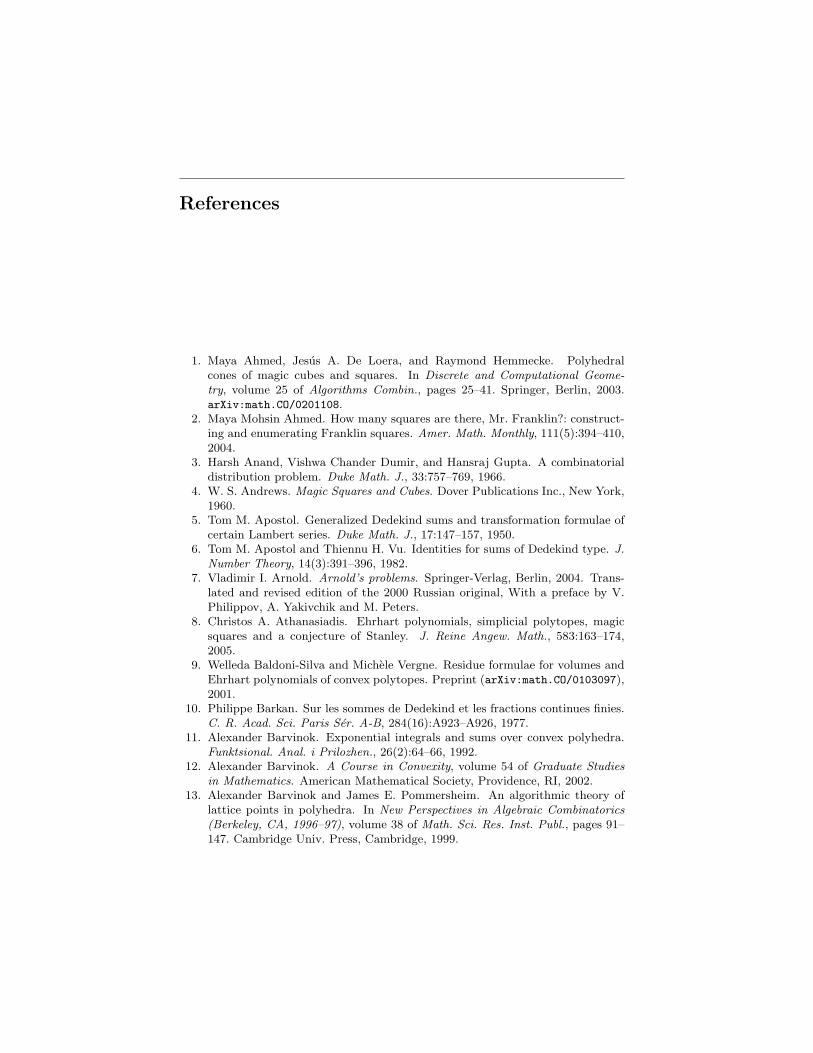
References
1. Maya Ahmed, Jesus A. De Loera, and Raymond Hemmecke. Polyhedralcones of magic cubes and squares. In Discrete and Computational Geome-try, volume 25 of Algorithms Combin., pages 25–41. Springer, Berlin, 2003.arXiv:math.CO/0201108.
2. Maya Mohsin Ahmed. How many squares are there, Mr. Franklin?: construct-ing and enumerating Franklin squares. Amer. Math. Monthly, 111(5):394–410,2004.
3. Harsh Anand, Vishwa Chander Dumir, and Hansraj Gupta. A combinatorialdistribution problem. Duke Math. J., 33:757–769, 1966.
4. W. S. Andrews. Magic Squares and Cubes. Dover Publications Inc., New York,1960.
5. Tom M. Apostol. Generalized Dedekind sums and transformation formulae ofcertain Lambert series. Duke Math. J., 17:147–157, 1950.
6. Tom M. Apostol and Thiennu H. Vu. Identities for sums of Dedekind type. J.Number Theory, 14(3):391–396, 1982.
7. Vladimir I. Arnold. Arnold’s problems. Springer-Verlag, Berlin, 2004. Trans-lated and revised edition of the 2000 Russian original, With a preface by V.Philippov, A. Yakivchik and M. Peters.
8. Christos A. Athanasiadis. Ehrhart polynomials, simplicial polytopes, magicsquares and a conjecture of Stanley. J. Reine Angew. Math., 583:163–174,2005.
9. Welleda Baldoni-Silva and Michele Vergne. Residue formulae for volumes andEhrhart polynomials of convex polytopes. Preprint (arXiv:math.CO/0103097),2001.
10. Philippe Barkan. Sur les sommes de Dedekind et les fractions continues finies.C. R. Acad. Sci. Paris Ser. A-B, 284(16):A923–A926, 1977.
11. Alexander Barvinok. Exponential integrals and sums over convex polyhedra.Funktsional. Anal. i Prilozhen., 26(2):64–66, 1992.
12. Alexander Barvinok. A Course in Convexity, volume 54 of Graduate Studiesin Mathematics. American Mathematical Society, Providence, RI, 2002.
13. Alexander Barvinok and James E. Pommersheim. An algorithmic theory oflattice points in polyhedra. In New Perspectives in Algebraic Combinatorics(Berkeley, CA, 1996–97), volume 38 of Math. Sci. Res. Inst. Publ., pages 91–147. Cambridge Univ. Press, Cambridge, 1999.

216 References
14. Alexander Barvinok and Kevin Woods. Short rational generating functions forlattice point problems. J. Amer. Math. Soc., 16(4):957–979 (electronic), 2003.arXiv:math.CO/0211146.
15. Alexander I. Barvinok. A polynomial time algorithm for counting integralpoints in polyhedra when the dimension is fixed. Math. Oper. Res., 19(4):769–779, 1994.
16. Victor V. Batyrev. Dual polyhedra and mirror symmetry for Calabi-Yauhypersurfaces in toric varieties. J. Algebraic Geom., 3(3):493–535, 1994.arXiv:alg-geom/9310003.
17. Victor V. Batyrev. Lattice polytopes with a given h∗-polynomial. In Al-gebraic and geometric combinatorics, volume 423 of Contemp. Math., pages1–10. Amer. Math. Soc., Providence, RI, 2006. arXiv:math.CO/0602593.
18. Victor V. Batyrev and Dimitrios I. Dais. Strong McKay correspondence, string-theoretic Hodge numbers and mirror symmetry. Topology, 35(4):901–929, 1996.
19. Matthias Beck. Counting lattice points by means of the residue theorem.Ramanujan J., 4(3):299–310, 2000. arXiv:math.CO/0306035.
20. Matthias Beck. Multidimensional Ehrhart reciprocity. J. Combin. Theory Ser.A, 97(1):187–194, 2002. arXiv:math.CO/0111331.
21. Matthias Beck. Dedekind cotangent sums. Acta Arith., 109(2):109–130, 2003.arXiv:math.NT/0112077.
22. Matthias Beck, Beifang Chen, Lenny Fukshansky, Christian Haase, Allen Knut-son, Bruce Reznick, Sinai Robins, and Achill Schurmann. Problems from theCottonwood Room. In Integer Points in Polyhedra—Geometry, Number The-ory, Algebra, Optimization, volume 374 of Contemp. Math., pages 179–191.Amer. Math. Soc., Providence, RI, 2005.
23. Matthias Beck, Moshe Cohen, Jessica Cuomo, and Paul Gribelyuk. Thenumber of “magic” squares, cubes, and hypercubes. Amer. Math. Monthly,110(8):707–717, 2003. arXiv:math.CO/0201013.
24. Matthias Beck, Jesus A. De Loera, Mike Develin, Julian Pfeifle, and Richard P.Stanley. Coefficients and roots of Ehrhart polynomials. In Integer Pointsin Polyhedra—Geometry, Number Theory, Algebra, Optimization, volume 374of Contemp. Math., pages 15–36. Amer. Math. Soc., Providence, RI, 2005.arXiv:math.CO/0402148.
25. Matthias Beck, Ricardo Diaz, and Sinai Robins. The Frobenius problem, ra-tional polytopes, and Fourier-Dedekind sums. J. Number Theory, 96(1):1–21,2002. arXiv:math.NT/0204035.
26. Matthias Beck and Richard Ehrenborg. Ehrhart–Macdonald reciprocity ex-tended. Preprint (arXiv:math.CO/0504230), 2006.
27. Matthias Beck, Christian Haase, and Frank Sottile. Formulas of Brion,Lawrence, and Varchenko on rational generating functions for cones. Math.Intelligencer, 31(1):9–17, 2009. arXiv:math.CO/0506466.
28. Matthias Beck and Dennis Pixton. The Ehrhart polynomial ofthe Birkhoff polytope. Discrete Comput. Geom., 30(4):623–637, 2003.arXiv:math.CO/0202267.
29. Matthias Beck and Sinai Robins. Explicit and efficient formulas for the latticepoint count in rational polygons using Dedekind–Rademacher sums. DiscreteComput. Geom., 27(4):443–459, 2002. arXiv:math.CO/0111329.
30. Matthias Beck and Frank Sottile. Irrational proofs for three theorems of Stan-ley. European J. Combin., 28(1):403–409, 2007. arXiv:math.CO/0506315.
References 217
31. Matthias Beck and Thomas Zaslavsky. An enumerative geometry formagic and magilatin labellings. Ann. Comb., 10(4):395–413, 2006.arXiv:math.CO/0506315.
32. Dale Beihoffer, Jemimah Hendry, Albert Nijenhuis, and Stan Wagon. Fasteralgorithms for Frobenius numbers. Electron. J. Combin., 12(1):Research Paper27, 38 pp. (electronic), 2005.
33. Nicole Berline and Michele Vergne. Local Euler-Maclaurin formula for poly-topes. Mosc. Math. J., 7(3):355–386, 573, 2007. arXiv:math.CO/0507256.
34. Bruce C. Berndt. Reciprocity theorems for Dedekind sums and generalizations.Advances in Math., 23(3):285–316, 1977.
35. Bruce C. Berndt and Ulrich Dieter. Sums involving the greatest integer func-tion and Riemann-Stieltjes integration. J. Reine Angew. Math., 337:208–220,1982.
36. Bruce C. Berndt and Boon Pin Yeap. Explicit evaluations and reciprocitytheorems for finite trigonometric sums. Adv. in Appl. Math., 29(3):358–385,2002.
37. Christian Bey, Martin Henk, and Jorg M. Wills. Notes on the rootsof Ehrhart polynomials. Discrete Comput. Geom., 38(1):81–98, 2007.arXiv:math.MG/0606089.
38. Louis J. Billera and A. Sarangarajan. The combinatorics of permutation poly-topes. In Formal Power Series and Algebraic Combinatorics (New Brunswick,NJ, 1994), pages 1–23. Amer. Math. Soc., Providence, RI, 1996.
39. Garrett Birkhoff. Tres observaciones sobre el algebra lineal. Revista Faculdadde Ciencias Exactas, Puras y Aplicadas Universidad Nacional de Tucuman,Serie A (Matematicas y Fısica Teoretica), 5:147–151, 1946.
40. G. R. Blakley. Combinatorial remarks on partitions of a multipartite number.Duke Math. J., 31:335–340, 1964.
41. Alfred Brauer. On a problem of partitions. Amer. J. Math., 64:299–312, 1942.42. Benjamin Braun. Norm bounds for Ehrhart polynomial roots. Discrete Com-
put. Geom., 39(1-3):191–193, 2008. arXiv:math.CO/0602464.43. Henrik Bresinsky. Symmetric semigroups of integers generated by 4 elements.
Manuscripta Math., 17(3):205–219, 1975.44. Charles J. Brianchon. Theoreme nouveau sur les polyedres. J. Ecole (Royale)
Polytechnique, 15:317–319, 1837.45. Michel Brion. Points entiers dans les polyedres convexes. Ann. Sci. Ecole
Norm. Sup. (4), 21(4):653–663, 1988.46. Michel Brion and Michele Vergne. Residue formulae, vector partition functions
and lattice points in rational polytopes. J. Amer. Math. Soc., 10(4):797–833,1997.
47. Arne Brøndsted. An Introduction to Convex Polytopes, volume 90 of GraduateTexts in Mathematics. Springer-Verlag, New York, 1983.
48. Richard A. Brualdi and Peter M. Gibson. Convex polyhedra of doubly stochas-tic matrices. I. Applications of the permanent function. J. Combinatorial The-ory Ser. A, 22(2):194–230, 1977.
49. Richard A. Brualdi and Peter M. Gibson. Convex polyhedra of doubly stochas-tic matrices. III. Affine and combinatorial properties of Un. J. CombinatorialTheory Ser. A, 22(3):338–351, 1977.
50. Heinz Bruggesser and Peter Mani. Shellable decompositions of cells andspheres. Math. Scand., 29:197–205 (1972), 1971.
218 References
51. Daniel Bump, Kwok-Kwong Choi, Par Kurlberg, and Jeffrey Vaaler. A localRiemann hypothesis. I. Math. Z., 233(1):1–19, 2000.
52. Kristin A. Camenga. Vector spaces spanned by the angle sums of polytopes.Beitrage Algebra Geom., 47(2):447–462, 2006. arXiv:math.MG/0508629.
53. Schuyler Cammann. Old Chinese magic squares. Sinologica, 7:14–53, 1962.54. Schuyler Cammann. Islamic and Indian magic squares, Parts I and II. History
of Religions, 8:181–209; 271–299, 1969.55. Sylvain E. Cappell and Julius L. Shaneson. Euler-Maclaurin expansions for
lattices above dimension one. C. R. Acad. Sci. Paris Ser. I Math., 321(7):885–890, 1995.
56. Leonard Carlitz. Some theorems on generalized Dedekind sums. Pacific J.Math., 3:513–522, 1953.
57. John W. S. Cassels. An Introduction to the Geometry of Numbers. Classicsin Mathematics. Springer-Verlag, Berlin, 1997. Corrected reprint of the 1971edition.
58. Clara S. Chan, David P. Robbins, and David S. Yuen. On the volume of a cer-tain polytope. Experiment. Math., 9(1):91–99, 2000. arXiv:math.CO/9810154.
59. Beifang Chen. Weight functions, double reciprocity laws, and volume formulasfor lattice polyhedra. Proc. Natl. Acad. Sci. USA, 95(16):9093–9098 (elec-tronic), 1998.
60. Beifang Chen. Lattice points, Dedekind sums, and Ehrhart polynomials oflattice polyhedra. Discrete Comput. Geom., 28(2):175–199, 2002.
61. Beifang Chen and Vladimir Turaev. Counting lattice points of rational poly-hedra. Adv. Math., 155(1):84–97, 2000.
62. Louis Comtet. Advanced Combinatorics. D. Reidel Publishing Co., Dordrecht,enlarged edition, 1974.
63. Wolfgang Dahmen and Charles A. Micchelli. The number of solutions to linearDiophantine equations and multivariate splines. Trans. Amer. Math. Soc.,308(2):509–532, 1988.
64. Vladimir I. Danilov. The geometry of toric varieties. Uspekhi Mat. Nauk,33(2(200)):85–134, 247, 1978.
65. J. Leslie Davison. On the linear Diophantine problem of Frobenius. J. NumberTheory, 48(3):353–363, 1994.
66. Jesus A. De Loera, David Haws, Raymond Hemmecke, Peter Huggins, andRuriko Yoshida. A user’s guide for LattE v1.1, software package LattE. 2004.Electronically available at http://www.math.ucdavis.edu/∼latte/.
67. Jesus A. De Loera, Raymond Hemmecke, Jeremiah Tauzer, and RurikoYoshida. Effective lattice point counting in rational convex polytopes. J.Symbolic Comput., 38(4):1273–1302, 2004.
68. Jesus A. De Loera and Shmuel Onn. The complexity of three-waystatistical tables. SIAM J. Comput., 33(4):819–836 (electronic), 2004.arXiv:math.CO/0207200.
69. Jesus A. De Loera, Jorg Rambau, and Francisco Santos. Triangulations ofPoint Sets: Applications, Structures, Algorithms. Springer (to appear), 2006.
70. Richard Dedekind. Erlauterungen zu den Fragmenten xxviii. In CollectedWorks of Bernhard Riemann, pages 466–478. Dover Publ., New York, 1953.
71. Max Dehn. Die Eulersche Formel im Zusammenhang mit dem Inhalt in dernicht-euklidischen Geometrie. Math. Ann., 61:279–298, 1905.
72. Jozsef Denes and Anthony D. Keedwell. Latin Squares and Their Applications.Academic Press, New York, 1974.
References 219
73. Graham Denham. Short generating functions for some semigroup algebras.Electron. J. Combin., 10:Research Paper 36, 7 pp. (electronic), 2003.
74. Persi Diaconis and Anil Gangolli. Rectangular arrays with fixed margins. InDiscrete Probability and Algorithms (Minneapolis, MN, 1993), pages 15–41.Springer, New York, 1995.
75. Ricardo Diaz and Sinai Robins. Pick’s formula via the Weierstrass ℘-function.Amer. Math. Monthly, 102(5):431–437, 1995.
76. Ricardo Diaz and Sinai Robins. The Ehrhart polynomial of a lattice polytope.Ann. of Math. (2), 145(3):503–518, 1997.
77. Ulrich Dieter. Das Verhalten der Kleinschen Funktionen log σg,h(ω1, ω2)gegenuber Modultransformationen und verallgemeinerte Dedekindsche Sum-men. J. Reine Angew. Math., 201:37–70, 1959.
78. Ulrich Dieter. Cotangent sums, a further generalization of Dedekind sums. J.Number Theory, 18(3):289–305, 1984.
79. Eugene Ehrhart. Sur les polyedres rationnels homothetiques a n dimensions.C. R. Acad. Sci. Paris, 254:616–618, 1962.
80. Eugene Ehrhart. Sur les carres magiques. C. R. Acad. Sci. Paris Ser. A-B,277:A651–A654, 1973.
81. Eugene Ehrhart. Polynomes arithmetiques et methode des polyedres en com-binatoire. Birkhauser Verlag, Basel, 1977. International Series of NumericalMathematics, Vol. 35.
82. Gunter Ewald. Combinatorial Convexity and Algebraic Geometry, volume 168of Graduate Texts in Mathematics. Springer-Verlag, New York, 1996.
83. Leonid G. Fel and Boris Y. Rubinstein. Restricted partition function asBernoulli and Euler polynomials of higher order. Ramanujan J., 11(3):331–348, 2006. arXiv:math.NT/0304356.
84. William Fulton. Introduction to Toric Varieties, volume 131 of Annals of Math-ematics Studies. Princeton University Press, Princeton, NJ, 1993.
85. Stavros Garoufalidis and James E. Pommersheim. Values of zeta functions atnegative integers, Dedekind sums and toric geometry. J. Amer. Math. Soc.,14(1):1–23 (electronic), 2001.
86. Ewgenij Gawrilow and Michael Joswig. polymake: a framework for analyzingconvex polytopes. In Polytopes—combinatorics and computation (Oberwolfach,1997), volume 29 of DMV Sem., pages 43–73. Birkhauser, Basel, 2000. Softwarepolymake available at www.math.tu-berlin.de/polymake/.
87. Ira M. Gessel. Generating functions and generalized Dedekind sums. Electron.J. Combin., 4(2):Research Paper 11, approx. 17 pp. (electronic), 1997.
88. Jorgen P. Gram. Om rumvinklerne i et polyeder. Tidsskrift for Math. (Copen-hagen), 4(3):161–163, 1874.
89. Harold Greenberg. An algorithm for a linear Diophantine equation and aproblem of Frobenius. Numer. Math., 34(4):349–352, 1980.
90. Branko Grunbaum. Convex Polytopes, volume 221 of Graduate Texts in Math-ematics. Springer-Verlag, New York, second edition, 2003. Prepared and witha preface by Volker Kaibel, Victor Klee, and Gunter M. Ziegler.
91. Victor Guillemin. Riemann-Roch for toric orbifolds. J. Differential Geom.,45(1):53–73, 1997.
92. Ulrich Halbritter. Some new reciprocity formulas for generalized Dedekindsums. Results Math., 8(1):21–46, 1985.
93. Richard R. Hall, J. C. Wilson, and Don Zagier. Reciprocity formulae for generalDedekind–Rademacher sums. Acta Arith., 73(4):389–396, 1995.
220 References
94. Martin Henk, Achill Schurmann, and Jorg M. Wills. Ehrhart polyno-mials and successive minima. Mathematika, 52(1-2):1–16 (2006), 2005.arXiv:math.MG/0507528.
95. Jurgen Herzog. Generators and relations of abelian semigroups and semigrouprings. Manuscripta Math., 3:175–193, 1970.
96. Takayuki Hibi. Algebraic Combinatorics on Convex Polytopes. Carslaw, 1992.97. Takayuki Hibi. Dual polytopes of rational convex polytopes. Combinatorica,
12(2):237–240, 1992.98. Takayuki Hibi. A lower bound theorem for Ehrhart polynomials of convex
polytopes. Adv. Math., 105(2):162–165, 1994.99. Dean Hickerson. Continued fractions and density results for Dedekind sums.
J. Reine Angew. Math., 290:113–116, 1977.100. Friedrich Hirzebruch. Neue topologische Methoden in der algebraischen Ge-
ometrie. Ergebnisse der Mathematik und ihrer Grenzgebiete (N.F.), Heft 9.Springer-Verlag, Berlin, 1956.
101. Friedrich Hirzebruch and Don Zagier. The Atiyah-Singer Theorem and Ele-mentary Number Theory. Publish or Perish Inc., Boston, Mass., 1974.
102. Jeffrey Hood and David Perkinson. Some facets of the polytope of even per-mutation matrices. Linear Algebra Appl., 381:237–244, 2004.
103. Masa-Nori Ishida. Polyhedral Laurent series and Brion’s equalities. Internat.J. Math., 1(3):251–265, 1990.
104. Maruf Israilovich Israilov. Determination of the number of solutions of lin-ear Diophantine equations and their applications in the theory of invariantcubature formulas. Sibirsk. Mat. Zh., 22(2):121–136, 237, 1981.
105. Ravi Kannan. Lattice translates of a polytope and the Frobenius problem.Combinatorica, 12(2):161–177, 1992.
106. Jean-Michel Kantor and Askold G. Khovanskiı. Une application du theoremede Riemann-Roch combinatoire au polynome d’Ehrhart des polytopes entiersde Rd. C. R. Acad. Sci. Paris Ser. I Math., 317(5):501–507, 1993.
107. Yael Karshon, Shlomo Sternberg, and Jonathan Weitsman. The Euler-Maclaurin formula for simple integral polytopes. Proc. Natl. Acad. Sci. USA,100(2):426–433 (electronic), 2003.
108. Askold G. Khovanskiı and Aleksandr V. Pukhlikov. The Riemann-Roch theo-rem for integrals and sums of quasipolynomials on virtual polytopes. Algebrai Analiz, 4(4):188–216, 1992.
109. Peter Kirschenhofer, Attila Petho, and Robert F. Tichy. On analytical andDiophantine properties of a family of counting polynomials. Acta Sci. Math.(Szeged), 65(1-2):47–59, 1999.
110. Daniel A. Klain and Gian-Carlo Rota. Introduction to Geometric Probability.Lezioni Lincee. Cambridge University Press, Cambridge, 1997.
111. Victor Klee. A combinatorial analogue of Poincare’s duality theorem. Canad.J. Math., 16:517–531, 1964.
112. Donald E. Knuth. Permutations, matrices, and generalized Young tableaux.Pacific J. Math., 34:709–727, 1970.
113. Donald E. Knuth. Notes on generalized Dedekind sums. Acta Arith., 33(4):297–325, 1977.
114. Donald E. Knuth. The Art of Computer Programming. Vol. 2. Addison-WesleyPublishing Co., Reading, Mass., second edition, 1981.

References 221
115. Matthias Koppe. A primal Barvinok algorithm based on irrationaldecompositions. SIAM J. Discrete Math., 21(1):220–236 (electronic),2007. arXiv:math.CO/0603308. Software LattE macchiato available athttp://www.math.uni-magdeburg.de/∼mkoeppe/latte/.
116. Thomas W. Korner. Fourier Analysis. Cambridge University Press, Cam-bridge, 1988.
117. Maximilian Kreuzer and Harald Skarke. Classification of reflexive poly-hedra in three dimensions. Adv. Theor. Math. Phys., 2(4):853–871, 1998.arXiv:hep-th/9805190.
118. Maximilian Kreuzer and Harald Skarke. Complete classification of reflexivepolyhedra in four dimensions. Adv. Theor. Math. Phys., 4(6):1209–1230, 2000.arXiv:hep-th/0002240.
119. Jean B. Lasserre and Eduardo S. Zeron. On counting integral points in aconvex rational polytope. Math. Oper. Res., 28(4):853–870, 2003.
120. Jim Lawrence. A short proof of Euler’s relation for convex polytopes. Canad.Math. Bull., 40(4):471–474, 1997.
121. Arjen K. Lenstra, Hendrik W. Lenstra, Jr., and Laszlo Lovasz. Factoringpolynomials with rational coefficients. Math. Ann., 261(4):515–534, 1982.
122. Laszlo Lovasz. Combinatorial Problems and Exercises. North-Holland Pub-lishing Co., Amsterdam, second edition, 1993.
123. Ian G. Macdonald. Polynomials associated with finite cell-complexes. J. Lon-don Math. Soc. (2), 4:181–192, 1971.
124. Percy A. MacMahon. Combinatory Analysis. Chelsea Publishing Co., NewYork, 1960.
125. Evgeny N. Materov. The Bott formula for toric varieties. Mosc. Math. J.,2(1):161–182, 2002. arXiv:math.AG/9904110.
126. Tyrrell B. McAllister and Kevin M. Woods. The minimum period of theEhrhart quasi-polynomial of a rational polytope. J. Combin. Theory Ser. A,109(2):345–352, 2005. arXiv:math.CO/0310255.
127. Peter McMullen. Valuations and Euler-type relations on certain classes ofconvex polytopes. Proc. London Math. Soc. (3), 35(1):113–135, 1977.
128. Peter McMullen. Lattice invariant valuations on rational polytopes. Arch.Math. (Basel), 31(5):509–516, 1978/79.
129. Curt Meyer. Uber einige Anwendungen Dedekindscher Summen. J. ReineAngew. Math., 198:143–203, 1957.
130. Jeffrey L. Meyer. Character analogues of Dedekind sums and transformationsof analytic Eisenstein series. Pacific J. Math., 194(1):137–164, 2000.
131. Werner Meyer and Robert Sczech. Uber eine topologische und zahlentheoretis-che Anwendung von Hirzebruchs Spitzenauflosung. Math. Ann., 240(1):69–96,1979.
132. Ezra Miller and Bernd Sturmfels. Combinatorial Commutative Algebra, volume227 of Graduate Texts in Mathematics. Springer-Verlag, New York, 2005.
133. Hermann Minkowski. Geometrie der Zahlen. Bibliotheca Mathematica Teub-neriana, Band 40. Johnson Reprint Corp., New York, 1968.
134. Marcel Morales. Syzygies of monomial curves and a linear Diophantine problemof Frobenius. Preprint, Max-Planck-Institut fur Mathematik, Bonn, 1986.
135. Marcel Morales. Noetherian symbolic blow-ups. J. Algebra, 140(1):12–25, 1991.136. Louis J. Mordell. Lattice points in a tetrahedron and generalized Dedekind
sums. J. Indian Math. Soc. (N.S.), 15:41–46, 1951.
222 References
137. Robert Morelli. Pick’s theorem and the Todd class of a toric variety. Adv.Math., 100(2):183–231, 1993.
138. Gerald Myerson. On semiregular finite continued fractions. Arch. Math.(Basel), 48(5):420–425, 1987.
139. Walter Nef. Zur Einfuhrung der Eulerschen Charakteristik. Monatsh. Math.,92(1):41–46, 1981.
140. C. D. Olds, Anneli Lax, and Giuliana P. Davidoff. The Geometry of Numbers,volume 41 of Anneli Lax New Mathematical Library. Mathematical Associationof America, Washington, DC, 2000.
141. Paul C. Pasles. The lost squares of Dr. Franklin: Ben Franklin’s missing squaresand the secret of the magic circle. Amer. Math. Monthly, 108(6):489–511, 2001.
142. Micha A. Perles and Geoffrey C. Shephard. Angle sums of convex polytopes.Math. Scand., 21:199–218 (1969), 1967.
143. Georg Alexander Pick. Geometrisches zur Zahlenlehre. Sitzenber. Lotos(Prague), 19:311–319, 1899.
144. Clifford A. Pickover. The Zen of Magic Squares, Circles, and Stars. PrincetonUniversity Press, Princeton, NJ, 2002.
145. Christopher Polis. Pick’s theorem extended and generalized. Math. Teacher,pages 399–401, 1991.
146. James E. Pommersheim. Toric varieties, lattice points and Dedekind sums.Math. Ann., 295(1):1–24, 1993.
147. Bjorn Poonen and Fernando Rodriguez-Villegas. Lattice polygons and thenumber 12. Amer. Math. Monthly, 107(3):238–250, 2000.
148. Tiberiu Popoviciu. Asupra unei probleme de patitie a numerelor. Acad. Re-publicii Populare Romane, Filiala Cluj, Studii si cercetari stiintifice, 4:7–58,1953.
149. Hans Rademacher. Generalization of the reciprocity formula for Dedekindsums. Duke Math. J., 21:391–397, 1954.
150. Hans Rademacher. Some remarks on certain generalized Dedekind sums. ActaArith., 9:97–105, 1964.
151. Hans Rademacher and Emil Grosswald. Dedekind Sums. The MathematicalAssociation of America, Washington, D.C., 1972.
152. Jorge L. Ramırez-Alfonsın. Complexity of the Frobenius problem. Combina-torica, 16(1):143–147, 1996.
153. Jorge L. Ramırez-Alfonsın. The Diophantine Frobenius Problem. Oxford Uni-versity Press, 2006.
154. J. E. Reeve. On the volume of lattice polyhedra. Proc. London Math. Soc. (3),7:378–395, 1957.
155. Les Reid and Leslie G. Roberts. Monomial subrings in arbitrary dimension. J.Algebra, 236(2):703–730, 2001.
156. Jurgen Richter-Gebert. Realization Spaces of Polytopes, volume 1643 of LectureNotes in Mathematics. Springer-Verlag, Berlin Heidelberg, 1996.
157. Boris Y. Rubinstein. An explicit formula for restricted partition functionthrough Bernoulli polynomials. Preprint, 2005.
158. Ludwig Schlafli. Theorie der vielfachen Kontinuitat. In Ludwig Schlafli,1814–1895, Gesammelte Mathematische Abhandlungen, Vol. I, pages 167–387.Birkhauser, Basel, 1950.
159. Alexander Schrijver. Combinatorial Optimization. Polyhedra and Efficiency.Vol. A–C, volume 24 of Algorithms and Combinatorics. Springer-Verlag,Berlin, 2003.

References 223
160. Paul R. Scott. On convex lattice polygons. Bull. Austral. Math. Soc.,15(3):395–399, 1976.
161. Sinan Sertoz. On the number of solutions of the Diophantine equation ofFrobenius. Diskret. Mat., 10(2):62–71, 1998.
162. Geoffrey C. Shephard. An elementary proof of Gram’s theorem for convexpolytopes. Canad. J. Math., 19:1214–1217, 1967.
163. Carl Ludwig Siegel. Lectures on the Geometry of Numbers. Springer-Verlag,Berlin, 1989. Notes by B. Friedman, rewritten by Komaravolu Chandrasekha-ran with the assistance of Rudolf Suter, with a preface by Chandrasekharan.
164. R. Jamie Simpson and Robert Tijdeman. Multi-dimensional versions of atheorem of Fine and Wilf and a formula of Sylvester. Proc. Amer. Math. Soc.,131(6):1661–1671 (electronic), 2003.
165. Neil J. A. Sloane. On-line encyclopedia of integer sequences.http://www.research.att.com/∼njas/sequences/index.html.
166. David Solomon. Algebraic properties of Shintani’s generating functions:Dedekind sums and cocycles on PGL2(Q). Compositio Math., 112(3):333–362,1998.
167. Duncan M. Y. Sommerville. The relation connecting the angle-sums and vol-ume of a polytope in space of n dimensions. Proc. Roy. Soc. London, Ser. A,115:103–119, 1927.
168. Richard P. Stanley. Linear homogeneous Diophantine equations and magiclabelings of graphs. Duke Math. J., 40:607–632, 1973.
169. Richard P. Stanley. Combinatorial reciprocity theorems. Advances in Math.,14:194–253, 1974.
170. Richard P. Stanley. Decompositions of rational convex polytopes. Ann. Dis-crete Math., 6:333–342, 1980.
171. Richard P. Stanley. Combinatorics and Commutative Algebra, volume 41 ofProgress in Mathematics. Birkhauser Boston Inc., Boston, MA, second edition,1996.
172. Richard P. Stanley. Enumerative Combinatorics. Vol. 1, volume 49 of Cam-bridge Studies in Advanced Mathematics. Cambridge University Press, Cam-bridge, 1997. With a foreword by Gian-Carlo Rota, Corrected reprint of the1986 original.
173. Bernd Sturmfels. On vector partition functions. J. Combin. Theory Ser. A,72(2):302–309, 1995.
174. Bernd Sturmfels. Grobner Bases and Convex Polytopes, volume 8 of UniversityLecture Series. American Mathematical Society, Providence, RI, 1996.
175. James J. Sylvester. On the partition of numbers. Quaterly J. Math., 1:141–152,1857.
176. James J. Sylvester. On subinvariants, i.e. semi-invariants to binary quantics ofan unlimited order. Amer. J. Math., 5:119–136, 1882.
177. James J. Sylvester. Mathematical questions with their solutions. EducationalTimes, 41:171–178, 1884.
178. Andras Szenes and Michele Vergne. Residue formulae for vector partitionsand Euler-MacLaurin sums. Adv. in Appl. Math., 30(1-2):295–342, 2003.arXiv:math.CO/0202253.
179. Lajos Takacs. On generalized Dedekind sums. J. Number Theory, 11(2):264–272, 1979.

224 References
180. Audrey Terras. Fourier Analysis on Finite Groups and Applications, volume 43of London Mathematical Society Student Texts. Cambridge University Press,Cambridge, 1999.
181. John A. Todd. The geometrical invariants of algebraic loci. Proc. LondonMath. Soc., 43:127–141, 1937.
182. John A. Todd. The geometrical invariants of algebraic loci (second paper).Proc. London Math. Soc., 45:410–424, 1939.
183. Amitabha Tripathi. The number of solutions to ax+by = n. Fibonacci Quart.,38(4):290–293, 2000.
184. Helge Tverberg. How to cut a convex polytope into simplices. GeometriaeDedicata, 3:239–240, 1974.
185. Sven Verdoolaege. Software package barvinok. 2004. Electronically availableat http://freshmeat.net/projects/barvinok/.
186. John von Neumann. A certain zero-sum two-person game equivalent to theoptimal assignment problem. In Contributions to the Theory of Games, vol.2, Annals of Mathematics Studies, no. 28, pages 5–12. Princeton UniversityPress, Princeton, N. J., 1953.
187. Herbert S. Wilf. generatingfunctionology. Academic Press Inc.,Boston, MA, second edition, 1994. Electronically available athttp://www.cis.upenn.edu/∼wilf/.
188. Kevin Woods. Computing the period of an Ehrhart quasi-polynomial. Electron.J. Combin., 12(1):Research Paper 34, 12 pp. (electronic), 2005.
189. Guoce Xin. Constructing all magic squares of order three. Discrete Math.,308(15):3393–3398, 2008. arXiv:math.CO/0409468.
190. Don Zagier. Higher dimensional Dedekind sums. Math. Ann., 202:149–172,1973.
191. Claudia Zaslavsky. Africa Counts. Prindle, Weber & Schmidt, Inc., Boston,Mass., 1973.
192. Doron Zeilberger. Proof of a conjecture of Chan, Robbins, and Yuen. Electron.Trans. Numer. Anal., 9:147–148 (electronic), 1999.
193. Gunter M. Ziegler. Lectures on polytopes. Springer-Verlag, New York,1995. Revised edition, 1998; “Updates, corrections, and more” atwww.math.tu-berlin.de/∼ziegler.

List of Symbols
The following table contains a list of symbols that are frequently used through-out the book. The page numbers refer to the first appearance/definition ofeach symbol.
Symbol Meaning Pagea(m) Fourier coefficient of a(n) 124A (d, k) Eulerian number 28A⊥ orthogonal complement of A 157AP(t) solid-angle sum of P 178αP(z) solid-angle generating function 180Bk(x) Bernoulli polynomial 31Bk Bernoulli number 32Bn Birkhoff polytope 106BiPyr (P) bipyramid over P 36coneP cone over P 56const f constant term of the generating function f 13convS convex hull of S 25d-cone d-dimensional cone 56d-polytope d-dimensional polytope 26dimP dimension of P 26δm(x) delta function 127EhrP(z) Ehrhart series of P 28EhrP◦(z) Ehrhart series of the interior of P 85ea(x) root-of-unity function e2πiax/b 127fk face number 93Fk(t) lattice-point enumerator of the k-skeleton 94F(f) Fourier transform of f 127g (a1, a2, . . . , ad) Frobenius number 6Hn(t) number of semimagic n× n squares with line sum t 105KF tangent cone of F ⊆ P 157

226 List of Symbols
Symbol Meaning PageLP(t) lattice-point enumerator of P 27LP◦(t) lattice-point enumerator of the interior of P 28Mn(t) number of magic n× n squares with line sum t 105ωP(x) solid angle of x (with respect to P) 177pA(n) restricted partition function 6polyA(n) polynomial part of pA(n) 139P a closed polytope 25P◦ interior of the polytope P 28P(h) perturbed polytope 172Pyr (P) pyramid over P 34℘(z) Weierstraß ℘-function 191Π fundamental parallelepiped of a cone 60rn(a, b) Dedekind–Rademacher sum 143s(a, b) Dedekind sum 126sn (a1, a2, . . . , am; b) Fourier–Dedekind sum 14SolidP(x) solid-angle series 186spanP affine space spanned by P 26σS(z) integer-point transform of S 58tP tth dilation of P 27Toddh Todd operator 166volP (continuous) volume of P 69VG vector space of all complex-valued functions 127
on G = {0, 1, 2, . . . , b− 1}ξa root of unity e2πi/a 8ζ(z) Weierstraß ζ-function 191bxc greatest integer function 10{x} fraction-part function 10((x)) sawtooth function 125(mn
)binomial coefficient 27
〈f, g〉 inner product of f and g 128(f ∗ g)(t) convolution of f and g 1311S(x) characteristic function of S 158#S number of elements in S 6♣ an exercise that is used in the text VIII
Index
affine space, 26affine span, 98apex, 56, 157area, 38arrangement of hyperplanes, 77, 157
Barvinok’s algorithm, 162basis, 127Beatty sequence, 20Bernoulli number, 32, 51, 165Bernoulli polynomial, 31, 52, 175binomial coefficient, 27binomial series, 30bipyramid over a polytope, 36Birkhoff–von Neumann polytope, 106,
116Boolean lattice, 94, 213boundary, 97Brianchon–Gram relation, 183, 187Brion’s theorem, 159
continuous form of, 168for solid angles, 181
complex conjugation, 128cone, 157
pointed, 56rational, 157simplicial, 56unimodular, 172
coning over a polytope, 56, 62, 73constituent, 44, 115contingency table, 117continuous Fourier transform, 133continuous volume, 69, 98, 107, 180
convex cone, 157convex hull, 25convex polygon, 25convex polytope, 25, 48convolution
of finite Fourier series, 131of quasipolynomials, 79
cotangent, 125cross-polytope, 35, 49cube, 26cyclotomic polynomial, 134
Dedekind η-function, 148Dedekind sum, 126, 130, 138, 145Dedekind’s reciprocity law, 141Dedekind–Rademacher sum, 143degenerate hyperplane, 26degree
of a polytope, 86of a quasipolynomial, 44
Dehn–Sommerville relations, 93delta function, 127, 134Delzant polytope, 172denominator, 73dihedral angle, 178dilate, 7dimension
of a pointed cone, 56of a polytope, 26
discrete volume, 27, 29, 36, 71, 81, 178distance, 128doubly periodic function, 191doubly stochastic matrix, 106

228 Index
dual polytope, 88
edgeof a pointed cone, 57of a polytope, 26
Ehrhart polynomial, 62, 65, 86, 96, 145constant term of, 68interpolation of, 71leading coefficient of, 70second coefficient of, 100
Ehrhart quasipolynomial, 73Ehrhart series, 28, 48, 66, 85, 147Ehrhart’s theorem, 62, 64, 73, 107Ehrhart–Macdonald reciprocity, 82, 94,
107, 143Euler φ-function, 134Euler characteristic, 75Euler relation, 94Eulerian number, 28, 48
facelattice, 94number, 93of a pointed cone, 57of a polytope, 26
facetof a pointed cone, 57of a polytope, 26
Farey sequence, 53Fibonacci sequence, 3, 150finite Fourier series, 121finite Fourier transform, 127finite geometric series, 17, 128, 153Fourier coefficient, 124Fourier transform, 127Fourier–Dedekind sum, 14, 137fractional-part function, 10, 18, 125frequency, 124Frobenius number, 6Frobenius problem, 3fundamental parallelepiped, 60
Gauß sum, 135gcd algorithm, 141, 145generating function, 3, 8, 13, 28, 58, 62,
109constant term of, 8, 13, 42, 115, 140,
146generator of a pointed cone, 56
geometric series, 4, 17, 60, 122graded algebra, 48greatest-integer function, 10, 17, 81, 125
h-cone, 197half-space, 26Hibi’s palindromic theorem, 86Hilbert–Poincare series, 48hyperplane, 26, 57
degenerate, 26rational, 77
hyperplane arrangement, 77, 157central, 157rational, 157
hyperplane description, 26, 48, 197hypersimplex, 77
indicator function, 158infinite sequence, 3inner product, 128, 134integer-point transform, 58, 63, 82, 153,
155of a simplicial cone, 60
integral polygon, 38integral polytope, 26, 62, 99, 186interior, 28, 81, 85
relative, 94, 107, 177interpolation, 70, 107isolated singularity, 189
Jacobi symbol, 148
Khovanskiı–Pukhlikov theorem, 173
Lagrange interpolation formula, 71Laguerre polynomial, 49latin square, 116lattice, 25, 74, 194lattice basis, 20lattice point, 19, 25, 33, 58lattice-point enumerator, 27, 45Laurent series, 8, 189line segment, 11, 19, 26linear Diophantine problem of
Frobenius, 6local Riemann hypothesis, 49Luo Shu square, 104
Mobius function, 135magic square, 104
Index 229
traditional, 104magic sum, 103metric space, 128moment, 170moment generating function, 58
northeast lattice path, 20
octahedron, 36order polytope, 49orthogonal complement, 157orthogonality relations, 128
palindromyof the Ehrhart series of a reflexive
polytope, 86of the solid-angle generating function,
186Parseval identity, 129part of a partition, 6partial fractions, 4, 8, 13, 43, 122, 139,
146partition, 6period, 44, 73periodic function, 44, 121, 127periodic sequence, 123permutation matrix, 107Pick’s theorem, 38, 193Plancherel theorem, 129pointed cone, 56, 157
rational, 56polar polytope, 88polygon, 25
integral, 38rational, 40, 45
polyhedron, 157polynomial, 27, 30, 33, 40, 62, 68–70,
76, 99, 107, 132, 153interpolation of, 71, 107
polytope, 7, 25Delzant, 172dual, 89integral, 26, 62, 99, 186normal, 48polar, 89rational, 26, 45, 73, 180simple, 93, 168smooth, 172unimodular, 172
Popoviciu’s theorem, 11power series, 8primitive root of unity, 134pyramid, 33, 49, 185
over a polytope, 34
quasipolynomial, 44, 73, 78, 114, 180constituent of, 44, 115degree of, 44period of, 44, 73
Rademacher reciprocity, 142rational pointed cone, 56rational polygon, 40, 45rational polytope, 26, 45, 73, 180reciprocity law
for the classical Dedekind sum, 141for the Dedekind–Rademacher sum,
143for the Fourier–Dedekind sum, 140,
142reciprocity theorem
for integer-point transforms, 84for lattice-point enumeration, 82for solid-angle generating functions,
181for solid-angle sums, 182
regular tetrahedron, 51, 187relative interior, 94, 107, 177relative volume, 98representable, 6residue, 189residue theorem, 190restricted partition function, 6, 13, 139
polynomial part of, 139Riemann zeta function, 32root, 69root of unity, 8
primitive, 134
sawtooth function, 125, 144semigroup, 76semimagic square, 104
symmetric, 118shelling, 100simple polytope, 93, 168simplex, 26, 55, 73
faces of, 50simplicial cone, 56
230 Index
skewed orthants, 155slack variable, 29, 42, 45smooth polytope, 172solid angle, 177
generating function, 180of a face, 177polynomial, 183series, 186sum of, 179
standard simplex, 29, 178Stanley’s nonnegativity theorem, 66Stanley’s reciprocity theorem, 84Stirling number of the first kind, 31, 51sublattice, 98supporting hyperplane, 26, 57Sylvester’s theorem, 6symmetric semimagic square, 118
tangent cone, 157tetrahedron, 26, 146Todd operator, 166, 172toric variety, 48traditional magic square, 104transportation polytope, 117triangle, 20, 26, 41triangulation
of a pointed cone, 58
of a polygon, 39of a polytope, 55, 203
trigonometric identities, 131trivial, 113
unimodularcone, 172polytope, 172
unit cube, 26, 33unitary transformation, 133
v-cone, 197valuation, 187Vandermonde matrix, 77vector partition function, 49vector space, 127vertex, 26, 117vertex cone, 157vertex description, 25, 48, 197visible, 204volume, 26, 69, 81, 98, 107, 172, 180
Weierstraß ℘-function, 191Weierstraß ζ-function, 191
Zagier reciprocity, 140zero, 183


