Contents lists available at SciVerse ScienceDirect
Journal of Symbolic Computation
journal homepage: www.elsevier.com/locate/jsc
Computing the multiplicity structure of an isolated singularsolution: Case of breadth oneNan Li, Lihong ZhiKey Lab of Mathematics Mechanization, AMSS, Chinese Academy of Sciences, Beijing 100190, China
a r t i c l e i n f o
Article history:Received 31 October 2009Accepted 13 March 2010Available online 22 December 2011
Keywords:Polynomial systemIsolated singular solutionMultiplicity structureLocal dual spaceCorank one
a b s t r a c t
We present an explicit algorithm to compute a closed basis of thelocal dual space of I = ( f1, . . . , ft) at a given isolated singularsolution x = (x1, . . . , xs) when the Jacobian matrix J(x) hascorank one. The algorithm is efficient both in time and memoryuse. Moreover, it can bemodified to compute an approximate basisif the coefficients of f1, . . . , ft and x are only known with limitedaccuracy.
Motivation and problem statement. Consider an ideal I generated by a polynomial system F =
{ f1, . . . , ft}, where fi ∈ C[x1, . . . , xs], i = 1, . . . , t . For a given isolated singular solution x =
(x1, . . . , xs) of F , suppose Q is the isolated primary component whose associate prime is P = (x1 −
x1, . . . , xs−xs). In (Wu and Zhi, 2008), we used the symbolic–numericmethod based on the geometricjet theory of partial differential equations introduced in (Reid et al., 2003; Zhi and Reid, 2004; Bonasiaet al., 2004) to compute the index ρ, the minimal nonnegative integer such that Pρ
⊆ Q , and themultiplicity µ = dim(C[x]/Q ), where Q = (I, Pρ). A basis for the local dual space of I at x isobtained from the null space of the truncated coefficient matrix of the involutive system. The sizeof these coefficient matrices is bounded by t
ρ+ss
×
ρ+ss
which will be very big when ρ or s is large.
In general, ρ ≤ µ. However, when the corank of the Jacobian matrix is one, then ρ = µ, which is alsocalled the breadth one case in (Dayton and Zeng, 2005; Dayton et al., 2009). The size of the matricesgrows extremely fast with the multiplicity µ. As pointed out in (Zeng, 2009), the matrix size becomesthe main bottleneck that slows down the overall computation. This is the main motivation for us toconsider whether we can compute the multiplicity structure of x efficiently in this worst case.
In (Dayton and Zeng, 2005; Dayton et al., 2009), they presented an efficient algorithm forcomputing a dual basis for the breadth one case by solving a deflated system of size roughly (µt) ×
N. Li, L. Zhi / Journal of Symbolic Computation 47 (2012) 700–710 701
(µs). A general construction of a Gauss basis of differential conditions at a multiple point was alsogiven in (Marinari et al., 1996, Section 4.3), the breadth one case is just a special case. The size of linearsystems they constructed is bounded by (µt) × (µs), and they assumed that I is a zero dimensionalsystem. In (Stetter, 2004, Section 8.5), an algorithmic approach for determining a basis of the local dualspace incrementally was stated and some examples were given to show that only a sizable number offree parameters are needed when we compute the k-th order differential condition.
Main contribution. In the breadth one case, following Stetter’s arguments and smart strategies givenin (Stetter, 2004, Section 8.5), we prove that the number of free parameters used in computingeach order of the differential condition of I at x can be reduced to s − 1. So that we can computethe multiplicity structure of an isolated multiple zero x very efficiently by solving µ − 2 linearsystems with size bounded by t × (s − 1). Moreover, during the computation, we only need to storepolynomials, the LU decomposition of the last s−1 columns of the Jacobianmatrix and the computeddifferential operators. Therefore, in the breadth one case, both storage space and execution time forcomputing a closed basis of the local dual space are reduced significantly. Furthermore, we modifythe algorithm for computing an approximate basis when singular solutions and polynomials are onlyknown approximately.
Structure of the paper. Section 2 is devoted to recalling some notations and well-known facts.In Section 3, we prove that for the breadth one case, a closed basis of the local dual space of Iat x can be constructed incrementally by checking whether a differential operator parameterizedby s − 1 variables is consistent with polynomials in I . In Section 4, we describe an algorithm forcomputing a closed basis of the local dual space of I at x and the multiplicity µ. If I and x are onlyknown with limited accuracy, then we modify the symbolic algorithm by introducing one moreparameter and using singular value decomposition or LU decomposition with pivoting to ensure thenumeric stability of the algorithm. Three examples are given to demonstrate that our algorithms areapplicable to positive dimensional systems, analytic systems and polynomial systems with irrationalor approximate coefficients. The complexity analysis and experiments are done in Section 5. Wemention some ongoing research in Section 6.
2. Preliminaries
Suppose we are given an isolated multiple root x of the polynomial system F = { f1, . . . , ft} withmultiplicity µ and index ρ.
Let D(α) = D(α1, . . . , αs) : C[x] → C[x] denote the differential operator defined by:
D(α1, . . . , αs) :=1
α1! · · · αs!∂xα1
1 · · · ∂xαss ,
for non-negative integer array α = [α1, . . . , αs]. We write D = {D(α), |α| ≥ 0} and denote bySpanC(D) the C-vector space generated by D and introduce a morphism on D that acts as ‘‘integral’’:
As a counterpart of the anti-differentiation operator Φj, we define the differentiation operator Ψjas
Ψj(D(α)) := D(α1, . . . , αj + 1, . . . , αs).
Definition 1. Given a zero x = (x1, . . . , xs) of an ideal I = ( f1, . . . , ft), we define the local dual spaceof I at x as
△x(I) := {L ∈ SpanC(D)| L( f )|x=x = 0, ∀f ∈ I}. (1)The vector space △x(I) and conditions equivalent to L( f )|x=x = 0, ∀L ∈ △x(I) are also called MaxNoether space and Max Noether conditions in Möller and Tenberg (2001) respectively.
For a non-negative integer k,△(k)x (I) consists of differential operators in△x(I)with the differential
order bounded by k. We have that dimC(△x(I)) = µ, where µ is the multiplicity of the zero x.
702 N. Li, L. Zhi / Journal of Symbolic Computation 47 (2012) 700–710
Definition 2. A subspace △x of SpanC(D) is said to be closed, if its dimension is finite, and if
L ∈ △x =⇒ Φj(L) ∈ △x, j = 1, . . . , s. (2)
Suppose Span(L0, L1, . . . , Lµ−1) is closed and L0, . . . , Lµ−1 are linearly independent differentialoperators satisfy that Li( fj)|x=x = 0, j = 1, . . . , t, i = 0, . . . , µ − 1, then due to the closedness,Li(q · fj)|x=x = 0, ∀q ∈ C[x1, . . . , xs]. Hence, △x(I) = Span(L0, L1, . . . , Lµ−1).
Remark 2.1. Suppose △x(I) = Span(L0, L1, . . . , Lµ−1), then {L0,x, . . . , Lµ−1,x} is a dual basis of thelocal dual space of I at x, where Li,x( f ) := Li( f )|x=x. Hence, for simplicity, in the following context,we only show how to compute a closed basis of the local dual space of I at x.
Lemma 2.2. Let J(x) be the Jacobian matrix of a polynomial system F = { f1, . . . , ft} evaluated atx. Suppose the corank of J(x) is one, i.e., the dimension of its null space is one, then dim(△
(k)x (I)) =
dim(△(k−1)x (I)) + 1 for 1 ≤ k ≤ µ − 1 and dim(△
(k)x (I)) = dim(△
(µ−1)x (I)), for k ≥ µ. Hence µ = ρ .
Proof. Lemma 2.2 is an immediate consequence of (Stanley, 1973, Theorem 2.2) and (Dayton andZeng, 2005, Lemma 1). �
3. The local dual space of breadth one
In this section, we are mainly interested in computing a closed basis of the local dual space △x(I)when the corank of the Jacobian matrix J(x) is one. In (Stetter, 2004, Section 8.5), an algorithmicapproach for determining a basis of the local dual space incrementally was stated and some exampleswere given to show that only a sizable number of free parameters are needed when we compute thek-th order differential condition. It is very interesting to see that in the breadth one case, the number offree parameters used in computing the k-th order differential condition following Stetter’s strategiescan be reduced to s − 1. We state below our main theorem.
Theorem 3.1. Suppose we are given an isolatedmultiple root x of the polynomial system F = { f1, . . . , ft}with multiplicity µ and the corank of the Jacobian matrix J(x) is one, and L1 = D(1, 0, . . . , 0) ∈ △
(1)x (I).
We can construct the k-th order differential condition incrementally for k from 2 to µ− 1 by the followingformula:
Here i1 = · · · = ij−1 = 0 means that we only pick up terms which do not contain derivatives in∂x1, . . . , ∂xj−1, and ai,j are known parameters appearing in Li for 2 ≤ i ≤ k − 1 and 2 ≤ j ≤ s.
The parameters ak,j, j = 2, . . . , s in (3) are determined by checking whether
[Pk( f1)|x=x, . . . , Pk( ft)|x=x]T
can be written as a linear combination of the last s−1 linearly independent columns of the JacobianmatrixJ(x).
Remark 3.2. It has been pointed out in (Stetter, 2004, Section 8.5) that if L1 ∈ △(1)x (I) is not
D(1, 0, . . . , 0) but a linear combination of ∂x1, . . . , ∂xs, then we can perform linear transformationof the variables which takes the vector of the linear combination into a unit vector (1, . . . , 0)T andreduces the situation to the one where L1 = D(1, 0, . . . , 0). However, the change of variables usuallywill destroy the sparsity structure of input polynomials and might be avoided by using directionalderivative (Apostol and Tom, 1974; Stetter, 2004).
N. Li, L. Zhi / Journal of Symbolic Computation 47 (2012) 700–710 703
Let us suppose now that the given isolated multiple root x of an ideal I = ( f1, . . . , ft) hasmultiplicity µ and the corank of its Jacobian matrix J(x) is one, and L0 = D(0, . . . , 0), L1 =
D(1, 0, . . . , 0) ∈ △(1)x (I). In the following, we show how to compute incrementally from L0, L1, a
closed set of linearly independent differential operators L2, . . . , Lµ−1 of derivative order 2, . . . , µ − 1respectively, and △x(I) = Span(L0, L1, L2, . . . , Lµ−1).
Lemma 3.3. Suppose {L0, . . . , Lµ−1} is a closed set of µ linearly independent differential operators whichform a basis of the local dual space△x(I), where the highest order derivative of Lk is k, then D(k, 0, . . . , 0)is the only term in Lk consisting of the k-th derivative.
Proof. The proof is done by induction on k. It is clear that Lemma 3.3 is true for k = 0, 1. Our inductiveassumption is that, Lk−1 has only one term D(k − 1, 0, . . . , 0) as the (k − 1)-th derivative, therefore,the k-th order differential operator which retains closedness can only be Ψj(D(k − 1, 0, . . . , 0)) for1 ≤ j ≤ s. However, when j = 1, Φ1
k−1(Ψj(D(k − 1, 0, . . . , 0))) = Ψj(D(0, . . . , 0)) which does notbelong to the subspace generated by {L0, L1} and violate the closedness condition. Hence, j = 1 andthe only k-th order derivative in Lk is D(k, 0, . . . , 0). �
According to Lemma 3.3, in the following, we suppose that
Lk = D(k, 0, . . . , 0) + {derivatives of order bounded by k − 1}.
Moreover, we assume that there are no terms D(i, 0, . . . , 0) for i < k appear in Lk, otherwise, we canreduce it by Li.
If ci,1 = 0, 0 ≤ i ≤ k − 2 then Φ1(Lk) must have the term D(i, 0, . . . , 0). Hence Lk has the termD(i + 1, 0, . . . , 0) for i ≤ k − 2 which contradicts the assumptions. Our claim follows for the firstequation.
The second equation is clear since the only k-th order derivative in Lk is D(k, 0, . . . , 0). We willprove later that ci,j for 1 ≤ i ≤ k − 2 are determined by {L0, . . . , Lk−1}. �
Proof of Theorem 3.1. Since
Pk = Ψ1(Φ1(Pk)) + {derivatives in Pk do not contain ∂ i1x1 for i1 > 0}
Therefore, formulas (4) and (5) are correct by setting Qj = Φj(Pk), 1 ≤ j ≤ s.
• For k = 2, it is clear that P2 = D(2, 0, . . . , 0) and (7) is correct.• For k = 3, suppose L3 = P3 + a3,2D(0, 1, 0, . . . , 0) + · · · + a3,sD(0, . . . , 1), where P3 consists of
derivatives of order at least two. By formula (6),
Φ1(P3) = Φ1(L3) = L2, Φj(P3) = c1,jL1, 2 ≤ j ≤ s.
If c1,j = 0, then the term D(1, 0, . . . , 1, . . . , 0) with 1 at positions 1 and j must appearin P3, moreover, due to the closedness, the term must be obtained by applying Ψ1 to L2 =
704 N. Li, L. Zhi / Journal of Symbolic Computation 47 (2012) 700–710
D(2, 0, . . . , 0) + a2,2D(0, 1, 0, . . . , 0) + · · · + a2,sD(0, . . . , 1) since L2 does not include the termD(1, 0, . . . , 0). Therefore
c1,j = a2,j, for 2 ≤ j ≤ s,
and (7) is correct for k = 3.• For k > 3, we assume the formula (7) is correct up to k − 1. According to (6), it is clear that
Similarly, if ci,j = 0, then Pk must have a term ci,jD(i, 0, . . . , 1, 0, . . . , 0)which has 1 at the positionj, for 2 ≤ j ≤ s. Moreover, to retain closedness, this term should come from Ψ1(Lk−1) since thereis no D(i, 0, . . . , 0) term in Lk−1 for 1 ≤ i ≤ k − 2. Hence the term ci,jD(i − 1, 0, . . . , 1, 0, . . . , 0)appears in Lk−1. If i = 1, then ci,j = ak−1,j = ak−i,j, otherwise, it must appear in Ψ1(Lk−2) accordingto (4), which implies that ci,jD(i − 2, 0, . . . , 1, 0, . . . , 0) should appear in Lk−2. In the same way,we can proceed further until Lk−i and get
ci,j = ak−i,j, for 2 ≤ j ≤ s.
Therefore, the formula (7) is correct for Φj(Pk), 1 ≤ j ≤ s.• The differential operator Lk defined by formulas (3)–(5) retains closedness and Lk ∈ △
(k)x (I) if
and only if the vector [Pk( f1)|x=x, . . . , Pk( ft)|x=x]T can be written as a linear combination of the
last s − 1 linear independent columns of the Jacobian matrix J(x). The values for the parametersak,j, j = 2, . . . , s can be determined if the linear combination does exist. Otherwise, we are finishedand the multiplicity of the root x is k. �
4. Algorithms for computing a basis of the local dual space
The routine MultiplicityStructureBreadthOneSymbolic below takes as input exact polynomialsF = { f1, . . . , ft} which generate an ideal I , an exact isolated solution x and the Jacobian matrix ofF evaluated at x has corank one, and returns the multiplicity µ and a closed basis L = {L0, . . . , Lµ−1}
of the local dual space of I at x.Algorithm 1. MultiplicityStructureBreadthOneSymbolicInput:An isolated singular solution x of a polynomial system F = { f1, . . . , ft}, and the Jacobianmatrixof F evaluated at x has corank one, L0 = D(0, 0, . . . , 0), L1 = D(1, 0, . . . , 0) ∈ △
(1)x (I).
Output: A closed basis L = {L0, . . . , Lµ−1} of the local dual space of I at x and the multiplicity µ.(1) Set k = 2 and P2 = D(2, 0, . . . , 0). Compute the LU decomposition of N which consists of the last
s − 1 columns of J(x). Suppose N = L · U .(2) Compute pk = [Pk( f1)|x=x, . . . , Pk( ft)|x=x]
T . If the triangular system L · bk = −pk is solvablethen solve the triangular system U · ak = bk to get ak = [ak,2, . . . , ak,s]T , set Lk = Pk +
ak,2D(0, 1, 0, . . . , 0) + · · · + ak,sD(0, . . . , 0, 1), and go to Step (3). Otherwise, go to Step (4).(3) Set k := k + 1, Pk = Ψ1(Lk−1) + Ψ2((Q2)i1=0) + · · · + Ψs((Qs)i1=i2=···=is−1=0), where Qj =
a2,jLk−2 + · · · + ak−1,jL1, for 2 ≤ j ≤ s, and go back to Step (2).(4) The algorithm returns {L0, L1, . . . , Lµ−1} as a basis of the local dual space of I at x and the
multiplicity µ = k.Remark 4.1. If L1 is not D(1, 0, . . . , 0), we compute a null vector of F ′(x), denoted by r1, and thenform a regular matrix R = [r1, . . . , rs]. By mapping x to Rz, we generate a new system H(z) = F(Rz),and applyMultiplicityStructureBreadthOneSymbolic to H and z = R−1x to get a closed basis. We mapit back to a closed basis of △x(I) by the following formula:
D(α) =1
α1! · · · αs!∂zα1
1 · · · ∂zαss
=1
α1! · · · αs!∂(rT1 · x)α1
· · · ∂(rTs · x)αs
=1
α1! · · · αs!
|β|=|α|
cβ · β1! · · · βs! · D(β).
N. Li, L. Zhi / Journal of Symbolic Computation 47 (2012) 700–710 705
InMaple implementation ofMultiplicityStructureBreadthOneSymbolic, we associate polynomialswiththe differential operators and this allows Ψj to be implemented as multiplication by xj. For example,we store L1 = D(1, 0, . . . , 0) as the polynomial x1 and store Ψj(L1) = D(1, 0, . . . , 0, 1, 0, . . . , 0) asx1xj.
Example 4.1 (Dayton, 2007). Consider a polynomial system
F = {2x2 − x − x3 + z3, x − y − x2 + xy + z2, xy2z − x2z − y2z + x3z}.
The system F has (0, 0, 0) as a 5-fold isolated solution, and there are also two other simple isolatedzeros but the ideal I defined by polynomials in F is not zero dimensional since the entire line {z =
0, x = 1} is a solution of F (Dayton, 2007).
Set x = [0, 0, 0]T and L0 = D(0, 0, 0). The Jacobian matrix of F evaluated at x is
J(x) =
−1 0 01 −1 00 0 0
which is annihilated by r1 =
001
.
We complete this column by r2 = [0, 1, 0]T , r3 = [1, 0, 0]T to form a regular 3 × 3-matrix R andgenerate a new polynomial system H(z) = F(Rz):
H = {2z2 − z − z3 + x3, z − y − z2 + yz + x2, xy2z − xz2 − xy2 + xz3}.
The Jacobian matrix of H evaluated at z = R−1x is
J(z) =
0 0 −10 −1 10 0 0
.
Initialize L1 = D(1, 0, 0), P2 = D(2, 0, 0), then we get p2 = [0, 1, 0]T . Solving
and p5 = [0, 0, −1]T . The fifth order differential operator consistent with closedness is
L5 = P5 + a5,2D(0, 1, 0) + a5,3D(0, 0, 1).
706 N. Li, L. Zhi / Journal of Symbolic Computation 47 (2012) 700–710
Since the last entry of p5 is nonzero, there are no parameters a5,2, a5,3 exist such that L5 is consistentwith H . So that we transform {L0, . . . , L4} back to a basis of the local dual space of I at x:
Notice that the matrix R only maps variables [x, y, z] to [z, y, x].If I and x are only known approximately, in order to compute an approximate closed basis of△x(I),
for ensuring the numerical stability, we need to add a free parameter to Pk and solve the resulted linearsystem using the singular value decomposition or LU decomposition with pivoting.Algorithm 2. MultiplicityStructureBreadthOneNumericInput: An isolated singular solution x of a polynomial system F = { f1, . . . , ft}, and the Jacobianmatrix of F evaluated at x has corank one with respect to a given tolerance τ , an approximate basisL0 = D(0, 0, . . . , 0), L1 = D(1, 0, . . . , 0) of △(1)
x (I).Output: A closed approximate basis L = {L0, . . . , Lµ−1} of the local dual space of I at x and themultiplicity µ.(1) Set k = 2, P2 = D(2, 0, . . . , 0), and N consists of the last s − 1 columns of J(x).(2) Compute pk = [Pk( f1)|x=x, . . . , Pk( ft)|x=x]
T . For the given tolerance τ , if the linear system[pk,N] · ak = 0 is solvable, we get ak = [ak,1, . . . , ak,s]T , set Lk = ak,1Pk + ak,2D(0, 1, 0, . . . , 0) +
· · · + ak,sD(0, . . . , 0, 1), and go to Step (3). Otherwise, go to Step (4).(3) Set k := k+1, Pk = Ψ1(Lk−1)+Ψ2((Q2)i1=0)+· · ·+Ψs((Qs)i1=i2=···=is−1=0), whereQj =
bk−2,jlk−2
Lk−2+
· · · +b1,jl1
L1. For 1 ≤ i ≤ k − 2 and 2 ≤ j ≤ s, bi,j is the coefficient of D(i, 0, . . . , 0, 1, 0, . . . , 0)in Ψ1(Lk−1), which has 1 at the position j, and li is the coefficient of D(i, 0, . . . , 0) in Li. Go back toStep (2).
(4) The algorithm returns {L0, L1, . . . , Lµ−1} as an approximate basis of the local dual space of I at xand the multiplicity µ = k.
Remark 4.2. In order to show the correctness of the algorithm MultiplicityStructureBreadthOneNu-meric, we need to check whether Qj in Step (3) is defined properly. Suppose D(i, 0, . . . , 0, 1, 0, . . . , 0)is a term in Ψ1(Lk−1) which has 1 at the position j for 1 ≤ i ≤ k− 2 and 2 ≤ j ≤ s, then D(i, 0, . . . , 0)must be a term in Φj(Pk)with the same coefficient, which is bi,j. On the other hand, by the formula (6)and Lemma 3.3, we have
Φj(Pk) = ck−2,jLk−2 + · · · + c1,jL1, 2 ≤ j ≤ s.Hence, the coefficient of D(i, 0, . . . , 0) in Φj(Pk) is ci,j · li. Therefore, from
bi,j = ci,j · li,
we derive that ci,j =bi,jli, for 1 ≤ i ≤ k − 2 and 2 ≤ j ≤ s.
In Step (2), suppose ak = [ak,1, . . . , ak,s]T is a null vector of [pk,N] with respect to the givetolerance τ , then we have
|Lk( fi)|x=x| ≤ τ , for 0 ≤ k ≤ µ − 1 and 1 ≤ i ≤ t.Moreover, according to our construction, all these computed Lk, 0 ≤ k ≤ µ − 1 satisfy the closednesscondition, hence, {L0, L1, . . . , Lµ−1} is a closed approximate basis of the local dual space of I at x.Example 4.2 (Dayton and Zeng, 2005). Consider the polynomial system
N. Li, L. Zhi / Journal of Symbolic Computation 47 (2012) 700–710 707
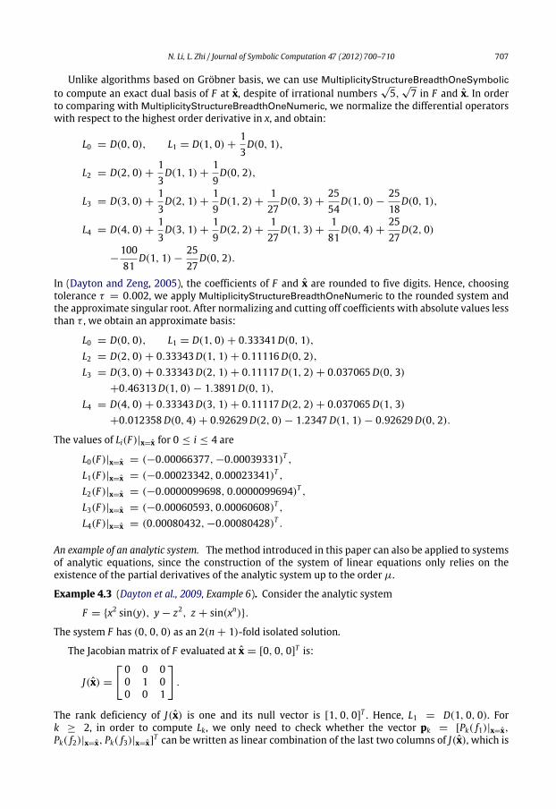
Unlike algorithms based on Gröbner basis, we can use MultiplicityStructureBreadthOneSymbolicto compute an exact dual basis of F at x, despite of irrational numbers
√5,
√7 in F and x. In order
to comparing with MultiplicityStructureBreadthOneNumeric, we normalize the differential operatorswith respect to the highest order derivative in x, and obtain:
L0 = D(0, 0), L1 = D(1, 0) +13D(0, 1),
L2 = D(2, 0) +13D(1, 1) +
19D(0, 2),
L3 = D(3, 0) +13D(2, 1) +
19D(1, 2) +
127
D(0, 3) +2554
D(1, 0) −2518
D(0, 1),
L4 = D(4, 0) +13D(3, 1) +
19D(2, 2) +
127
D(1, 3) +181
D(0, 4) +2527
D(2, 0)
−10081
D(1, 1) −2527
D(0, 2).
In (Dayton and Zeng, 2005), the coefficients of F and x are rounded to five digits. Hence, choosingtolerance τ = 0.002, we apply MultiplicityStructureBreadthOneNumeric to the rounded system andthe approximate singular root. After normalizing and cutting off coefficients with absolute values lessthan τ , we obtain an approximate basis:
An example of an analytic system. The method introduced in this paper can also be applied to systemsof analytic equations, since the construction of the system of linear equations only relies on theexistence of the partial derivatives of the analytic system up to the order µ.
Example 4.3 (Dayton et al., 2009, Example 6). Consider the analytic system
F = {x2 sin(y), y − z2, z + sin(xn)}.
The system F has (0, 0, 0) as an 2(n + 1)-fold isolated solution.
The Jacobian matrix of F evaluated at x = [0, 0, 0]T is:
J(x) =
0 0 00 1 00 0 1
.
The rank deficiency of J(x) is one and its null vector is [1, 0, 0]T . Hence, L1 = D(1, 0, 0). Fork ≥ 2, in order to compute Lk, we only need to check whether the vector pk = [Pk( f1)|x=x,Pk( f2)|x=x, Pk( f3)|x=x]
T can be written as linear combination of the last two columns of J(x), which is
708 N. Li, L. Zhi / Journal of Symbolic Computation 47 (2012) 700–710
equivalent to check whether the first entry of pk is zero. The dominant cost is the evaluation of Pk(F)at x. This can be done very efficiently since each polynomial in F only consists of one or two terms.Therefore, for this example, our algorithm MultiplicityStructureBreadthOneSymbolic is significantlyfaster and more powerful than the algorithm presented in (Dayton et al., 2009) (see Table 1).
Remark 4.3. The reviewer pointed out that for this analytic system, the local ring at (0, 0, 0) has basis{x2y, y − z2, z + xn} and the standard basis {y − z2, z + xn, x2n+2
} can be computed by Singular fromthe algebraic basis in negligible amount of time. From the degree of the variable x, we know that themultiplicity of (0, 0, 0) is 2n + 2.
5. Complexity and experiments
The complexity of algorithms MultiplicityStructureBreadthOneSymbolic and MultiplicityStructure-BreadthOneNumeric is dominated by solving µ − 2 linear systems with size bounded by t × s − 1 ort × s respectively, and the evaluations of
pk = [Pk( f1)|x=x, . . . , Pk( ft)|x=x]T .
Although we only need to store polynomials and the computed differential conditions during thecomputation, similar to other any algorithm designed to calculate and store the dual basis inmemory,our algorithm suffers toowhen polynomials or the differential operators are not sparse. The followingexample is kindly provided by the reviewer.
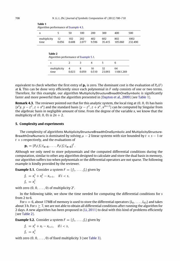
Example 5.1. Consider a system F = { f1, . . . , fs} given by
fi = x3i + x2i − xi+1, if i < s,
fs = x2swith zero (0, 0, . . . , 0) of multiplicity 2s.
In the following table, we show the time needed for computing the differential conditions for sfrom 2 to 6.
For s = 6, about 17MB of memory is used to store the differential operators {L0, . . . , L63} and takesabout 3 h. For s ≥ 7, we are not able to obtain all differential conditions after running the algorithm for2 days. A new algorithm has been proposed in (Li, 2011) to deal with this kind of problems efficiently(see Table 2).
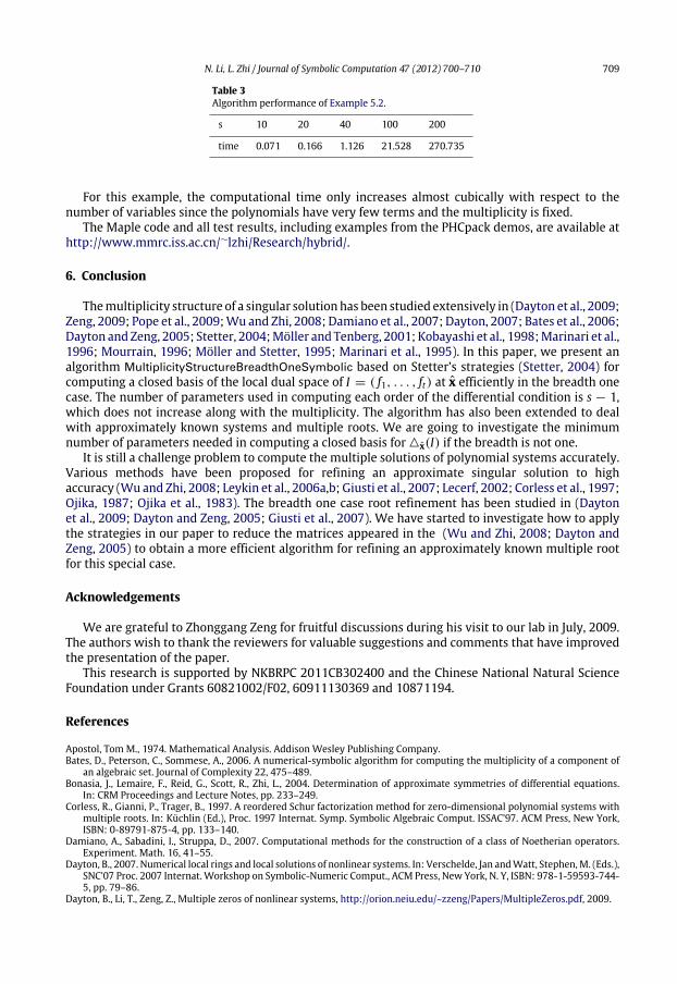
Example 5.2. Consider a system F = { f1, . . . , fs} given by
fi = x2i + xi − xi+1, if i < s,
fs = x3swith zero (0, 0, . . . , 0) of fixed multiplicity 3 (see Table 3).
N. Li, L. Zhi / Journal of Symbolic Computation 47 (2012) 700–710 709
Table 3Algorithm performance of Example 5.2.
s 10 20 40 100 200
time 0.071 0.166 1.126 21.528 270.735
For this example, the computational time only increases almost cubically with respect to thenumber of variables since the polynomials have very few terms and the multiplicity is fixed.
The Maple code and all test results, including examples from the PHCpack demos, are available athttp://www.mmrc.iss.ac.cn/∼lzhi/Research/hybrid/.
6. Conclusion
Themultiplicity structure of a singular solutionhas been studied extensively in (Dayton et al., 2009;Zeng, 2009; Pope et al., 2009;Wu and Zhi, 2008; Damiano et al., 2007; Dayton, 2007; Bates et al., 2006;Dayton and Zeng, 2005; Stetter, 2004;Möller and Tenberg, 2001; Kobayashi et al., 1998;Marinari et al.,1996; Mourrain, 1996; Möller and Stetter, 1995; Marinari et al., 1995). In this paper, we present analgorithm MultiplicityStructureBreadthOneSymbolic based on Stetter’s strategies (Stetter, 2004) forcomputing a closed basis of the local dual space of I = ( f1, . . . , ft) at x efficiently in the breadth onecase. The number of parameters used in computing each order of the differential condition is s − 1,which does not increase along with the multiplicity. The algorithm has also been extended to dealwith approximately known systems and multiple roots. We are going to investigate the minimumnumber of parameters needed in computing a closed basis for △x(I) if the breadth is not one.
It is still a challenge problem to compute the multiple solutions of polynomial systems accurately.Various methods have been proposed for refining an approximate singular solution to highaccuracy (Wu and Zhi, 2008; Leykin et al., 2006a,b; Giusti et al., 2007; Lecerf, 2002; Corless et al., 1997;Ojika, 1987; Ojika et al., 1983). The breadth one case root refinement has been studied in (Daytonet al., 2009; Dayton and Zeng, 2005; Giusti et al., 2007). We have started to investigate how to applythe strategies in our paper to reduce the matrices appeared in the (Wu and Zhi, 2008; Dayton andZeng, 2005) to obtain a more efficient algorithm for refining an approximately known multiple rootfor this special case.
Acknowledgements
We are grateful to Zhonggang Zeng for fruitful discussions during his visit to our lab in July, 2009.The authors wish to thank the reviewers for valuable suggestions and comments that have improvedthe presentation of the paper.
This research is supported by NKBRPC 2011CB302400 and the Chinese National Natural ScienceFoundation under Grants 60821002/F02, 60911130369 and 10871194.
References
Apostol, Tom M., 1974. Mathematical Analysis. Addison Wesley Publishing Company.Bates, D., Peterson, C., Sommese, A., 2006. A numerical-symbolic algorithm for computing the multiplicity of a component of
an algebraic set. Journal of Complexity 22, 475–489.Bonasia, J., Lemaire, F., Reid, G., Scott, R., Zhi, L., 2004. Determination of approximate symmetries of differential equations.
In: CRM Proceedings and Lecture Notes, pp. 233–249.Corless, R., Gianni, P., Trager, B., 1997. A reordered Schur factorization method for zero-dimensional polynomial systems with
multiple roots. In: Küchlin (Ed.), Proc. 1997 Internat. Symp. Symbolic Algebraic Comput. ISSAC’97. ACM Press, New York,ISBN: 0-89791-875-4, pp. 133–140.
Damiano, A., Sabadini, I., Struppa, D., 2007. Computational methods for the construction of a class of Noetherian operators.Experiment. Math. 16, 41–55.
Dayton, B., 2007. Numerical local rings and local solutions of nonlinear systems. In: Verschelde, Jan andWatt, Stephen,M. (Eds.),SNC’07 Proc. 2007 Internat.Workshop on Symbolic-Numeric Comput., ACM Press, New York, N. Y, ISBN: 978-1-59593-744-5, pp. 79–86.
710 N. Li, L. Zhi / Journal of Symbolic Computation 47 (2012) 700–710
Dayton, B., Zeng, Z., 2005. Computing the multiplicity structure in solving polynomial systems. In: Kauers, Manuel (Eds.),ISSAC’05 Proc. 2005 Internat. Symp. Symbolic Algebraic Comput., ACM Press, New York, N. Y, ISBN: 1-59593-095-7,pp. 116–123.
Giusti, M., Lecerf, G., Salvy, B., Yakoubsohn, J.-C., 2007. On location and approximation of clusters of zeros: Case of embeddingdimension one. Found. Comput. Math. (ISSN: 1615-3375) 7 (1), 1–58.
Kobayashi, H., Suzuki, H., Sakai, Y., 1998. Numerical calculation of the multiplicity of a solution to algebraic equations. Math.Comput. 67 (221), 257–270.
Lecerf, G., 2002. Quadratic Newton iteration for systems with multiplicity. Foundations of Computational Mathematics 2 (3),247–293.
Leykin, Anton, Verschelde, Jan, Zhao, Ailing, 2006a. Newton’s method with deflation for isolated singularities of polynomialsystems. Theoret. Comput. Sci. (ISSN: 0304-3975) 359 (1), 111–122.
Leykin, A., Verschelde, J., Zhao, A., 2006b. Newton’s method with deflation for isolated singularities of polynomial systems.Theoret. Comput. Sci. 359, 111–122.
Li, N., 2011. An improved method for evaluating Max Noether conditions: case of breadth one. In: Maza, M.M. (Ed.), SNC’11Proc. 2011 Internat. Workshop on Symbolic-Numeric Comput., ACM Press, New York, N. Y, pp. 102–103.
Marinari, M., Mora, T., Möller, H., 1995. Gröbner duality and multiplicities in polynomial solving. In: Levelt, A.H.M. (Ed.), Proc.1995 Internat. Symp. Symbolic Algebraic Comput. (ISSAC’95). ACM Press, New York, NY, pp. 167–179.
Marinari, M., Mora, T., Möller, H., 1996. Onmultiplicities in polynomial system solving. Trans. Amer.Math. Soc. 348, 3283–3321.Möller, H., Stetter, H., 1995. Multivariate polynomial equations with multiple zeros solved by matrix eigenproblems. Numer.
Math. 70, 311–329.Möller, H., Tenberg, R., 2001. Multivariate polynomial system solving using intersections of eigenspaces. J. Symbolic Comput.
30, 1–19.Mourrain, B., 1996. Isolated points, duality and residues. J. of Pure and Applied Algebra 117&118, 469–493.Ojika, T., 1987. Modified deflation algorithm for the solution of singular problems. J. Math. Anal. Appl. 123, 199–221.Ojika, T., Watanabe, S., Mitsui, T., 1983. Deflation algorithm for the multiple roots of a system of nonlinear equations. J. Math.
Anal. Appl. 96, 463–479.Pope, Scott R., Szanto Agnes, 2009. Nearest multivariate systemwith given rootmultiplicities. J. Symbolic Comput. (ISSN: 0747-
7171) 44 (6), 606–625.Reid, G., Tang, J., Zhi, L., 2003. A complete symbolic-numeric linear method for camera pose determination. In: Sendra, J. (Ed.),
Proc. 2003 Internat. Symp. Symbolic Algebraic Comput. ISSAC’03. ACM Press, New York, ISBN: 1-58113-641-2, pp. 215–223.Stanley, R.P., 1973. Hibert function of graded algebras. Advances in Math. 28, 57–83.Stetter, H., 2004. Numerical Polynomial Algebra. SIAM, Philadelphia.Wu, X., Zhi, L., 2008. Computing the multiplicity structure from geometric involutive form. In: Jeffrey, David (Eds.), Proc. 2008
Internat. Symp. Symbolic Algebraic Comput. (ISSAC’08). ACMPress, NewYork, N. Y, ISBN: 978-1-59593-904-3, pp. 325–332.Zeng, Z., The closedness subspace method for computing the multiplicity structure of a polynomial system.
http://orion.neiu.edu/~zzeng/Papers/csdual.pdf, 2009.Zhi, L., Reid, G., Solving nonlinear polynomial system via symbolic-numeric elimination method, In: Faugére, J. and Rouillier
F., Proc. International conference on polynomial system solving, pp. 50–53, 2004, Full version of the paper in J. SymoblicComput. 44(3), 280–291.