Concentration Profiles near an Activated Enzyme

Soohyung Park and Noam Agmon*Institute of Chemistry and the Fritz Haber Research Center, The Hebrew UniVersity, Jerusalem 91904, Israel

ReceiVed: May 2, 2008; ReVised Manuscript ReceiVed: June 25, 2008

When a resting enzyme is activated, substrate concentration profile evolves in its vicinity, ultimately tendingto steady state. We use modern theories for many-body effects on diffusion-influenced reactions to deriveapproximate analytical expressions for the steady-state profile and the Laplace transform of the transientconcentration profiles. These show excellent agreement with accurate many-particle Brownian-dynamicssimulations for the Michaelis-Menten kinetics. The steady-state profile has a hyperbolic dependence on thedistance of the substrate from the enzyme, albeit with a prefactor containing the complexity of the many-body effects. These are most conspicuous for the substrate concentration at the surface of the enzyme. Itshows an interesting transition as a function of the enzyme turnover rate. When it is high, the contactconcentration decays monotonically to steady state. However, for slow turnover it is nonmonotonic, showinga minimum due to reversible substrate binding, then a maximum due to diffusion of new substrate toward theenzyme, and finally decay to steady state. Under certain conditions one can obtain a good estimate for thecritical value of the turnover rate constant at the transition.

I. Introduction

The Michaelis-Menten (MM) mechanism1 is a widelyapplicable reaction scheme in biological processes. For enzy-matic reactions, this mechanism has been routinely applied tothe observed kinetics.2-7 MM kinetics was found to be ap-plicable even for single molecules, when the enzyme undergoeslarge conformational fluctuations.8-10 The classical descriptionof the MM kinetics ignores the many-body competition anddiffusion effects. These effects may be important in biologicalsystems, particularly inside the cell, when substrate diffusionis slowed down by microscopic obstacles even more than byviscosity.11,12

Modern theories of (many-body) diffusion-influenced reac-tions,13-23 which are successful in treating such effects inreversible reactions,24-28 have only recently been extended tothe MM mechanism.29-31 In a recent work,31 we have shownthat under general conditions the MM equation formally holds,albeit with a concentration-dependent Michaelis parameter, KM.The nonconstancy of this enzymatic “constant” is significantwhen the ratio of the catalytic and diffusion constants (kp/kD)is large.

Yet the above-mentioned theoretical treatments have focusedon the kinetics of product formation, whereas the spatio-temporaldistribution of diffusing substrate molecules received littleattention. For an irreversible reaction, the Smoluchowski theoryprovides analytic expressions for the concentration profilearound a reactive trap.32 Following activation of this trap, aconcentration gradient spreads out by diffusion, approachingits ultimate steady-state (SS) profile monotonically. In contrast,for the reversible A + Ba C (ABC) reaction, the concentrationof diffusing particles around the reaction site first decreases andthen restores its bulk value at long times.24,33 The MM schemeinvolves two steps, the first of which is reversible and thesecond, product formation step (rate constant kp), is irreversible.Thus both behaviors may be expected here.

The present work focuses on the time (t) evolution of theconcentration profile of substrate molecules around an enzymethat becomes activated at t ) 0. Utilizing the previouslydeveloped uniform theory31 for the MM kinetics, we obtain anaccurate theoretical description which is verified by Browniandynamics (BD) simulations. We treat both the spatial andtemporal dependence of the substrate concentration, from itsinitial uniform distribution and up to its final steady-state (SS)limit. A transition from monotonic to nonmonotonic approachto SS is observed as a function of kp. It is explainedquantitatively by the modern theories of diffusion-influencedreactions and qualitatively as competition between diffusion andenzymatic turnover, from which follows an approximate condi-tion for observing nonmonotonic behavior.

II. Theoretical Background

The MM mechanism is described as follows. In its first step,a free enzyme (A) and a substrate molecule (B) can associatewith the rate constant κ1, to form an enzyme-substrate complex(C). Then, this complex may redissociate into the enzyme andits substrate with the rate constant κ2, or proceed to the secondstep of product formation. In this step, the complex dissociateswith the rate-constant kp, into the product (P) and the originalenzyme (A). (kp is known as the “catalytic constant” or “turnovernumber”.) The reaction scheme is thus

A+B {\}κ1

κ2

C98kp

A+ P (2.1)

We assume that reaction between enzyme and substrate occursonly upon collision, at the contact distance, R. Interactionsbetween particles are ignored and the enzyme is assumed to bestatic, hence its diffusion constant vanishes (DA ) 0). This maynot be a bad approximation for a large biological molecule. Band P diffuse with the corresponding diffusion constants DB

and DP. However, P may be ignored because it is only aspectator in the reversible reaction.* Corresponding author. Email: agmon@fh.huji.ac.il.

J. Phys. Chem. B 2008, 112, 12104–1211412104

10.1021/jp803873p CCC: $40.75 2008 American Chemical SocietyPublished on Web 08/29/2008

We consider the MM mechanism in the pseudounimolecularlimit, when the bulk concentration of B is much larger thanthose of A and C. It can thus be regarded as a constant, b0. Theconcentrations of A and C vary with time: [A](t) and [C](t),while that of B varies both with time and its distance, r, fromA (or C): [B](r,t). As r f ∞, [B](r,t) f b0. The normalizedconcentrations of A and C are defined as

a(t) ≡ [A](t) ⁄ { [A](0) + [C](0)}

c(t) ≡ [C](t) ⁄ { [A](0) + [C](0)}

The normalized concentration profile of B is defined as b(r,t)≡ [B](r,t)/b0. We consider a system with an initially free enzymeembedded in a uniform substrate concentration, i.e., a(0) ≡ 1,c(0) ≡ 0, and b(r,0) ≡ 1.

A. Kinetic Hierarchy. From the reaction diffusion equationsfor the many-body joint probability distribution functions,34 onecan obtain evolution equations for an infinite hierarchy ofdistribution functions.13,14 These are obtained by integrating overall coordinates, all except one, two, etc. For the MM mechanism,the first two levels in the hierarchy can be written as

da(t)dt

)-dc(t)dt

)-κ1FAB(R, t)+ (κ2 + kp)c(t) (2.2a)

∂

∂tFAB(r, t)) LrFAB(r, t)- [κ1FAB(R, t)- κ2c(t)]

δ(r-R)

4πR2-

κ1FABB(r, R, t)+ (κ2 + kp)FCB(r, t) (2.2b)

∂

∂tFCB(r, t)) LrFCB(r, t)+ κ1FABB(r, R, t)- (κ2 + kp)FCB(r, t)

(2.2c)

where δ(x) is the Dirac delta function and Lr is the diffusionoperator, which is defined as

Lr ≡DB

r2

∂

∂rr2 ∂

∂r(2.3)

The diffusion constant in this operator is DB, because we haveassumed that A is static.

The AB pair distribution function, FAB(r,t), is defined asFAB(r,t) ≡ b0pAB(r,t), where pAB(r,t) is the probability densityof finding an AB pair separated by r at time t. In other words,FAB(r,t) is the concentration of B around the free trap, A, attime t. Similarly, FCB(r,t) is the concentration of B around theoccupied trap, C, at time t. The three-particle distributionfunction, FABB(r,r′,t), is similarly defined by FABB(r,r′,t) ≡b0

2pABB(r,r′,t), where pABB(r,r′,t) is the joint probability densityof finding two B particles at distances r and r′ from A at t.

The lowest level in the hierarchy, eq 2.2a, describes thekinetics of c(t). It is coupled to the second level via the reactivepair distribution, FAB(R,t). The second level of the hierarchy,eqs 2.2b and 2.2c, depict the evolution of the reactive andunreactive pair distributions, FAB(r,t) and FCB(r,t), respectively.These couple to the third level via the triplet density, FABB(r,R,t).Since we are interested here in the concentration profile of B,[B](r,t) ) FAB(r,t) + FCB(r,t), we need not go beyond the levelof doublets.

Initially, the pair distribution functions are given by FAB(r,0)) b0 and FCB(r,0) ) 0. Because reactions are introduced bysink terms, it is assumed that these functions obey a reflectingboundary condition at r ) R (and also at r ) ∞). Hence

∫R

∞d3r LrFAB(r, t))∫R

∞d3r LrFCB(r, t)) 0

Spatial integration of FAB(r,t) and FCB(r,t) gives b0a(t) and b0c(t),respectively. Similarly, integration of FABB(r,r′,t) over space with

respect to r′ (or r) gives b0FAB(r,t) [or b0FAB(r′,t)]. Thus eq 2.2ais obtained by integrating the higher level in the hierarchy, i.e.,eqs 2.2b and 2.2c.

The infinite hierarchy in eqs 2.2 is intractable and does notadmit an exact solution. Simple truncation of this hierarchy (e.g.,by writing higher order distribution functions as products oflower-order ones) usually does not give good results,particularly for the long-time asymptotic behavior. Therefore,we discuss another starting point, that of a rate-kernelequation which is formally equivalent to the full hierarchybut more amenable to approximations.14 However, we willreturn to the hierarchical equations when we discuss theconcentration profile in section III.

B. Memory Kernel. The starting point of our previous workwas the formally exact rate-kernel equation, which can beobtained from eqs 2.2:14

da(t)dt

)-dc(t)

dt)-κ1b0∫0

tdt ′ Σ(t- t ′ )a(t ′ )+

κ2∫0

tdt ′ Σ(t- t ′ )c(t ′ )+ kpc(t) (2.4)

where ∑(t) is a memory kernel which accounts for the historyof the repeated interactions in the reversible reaction. It maydepend on the rate constants, substrate concentration, diffusionconstant, and contact distance, but it is identical for bothdirections of the reversible reaction.

In Laplace space [f(s) ≡ ∫0∞ dt e-stf(t) for any function of

time, f(t)], the convolutions in eq 2.4 become multiplications.Inserting the Laplace transform (LT) of eq 2.4 into that of eq2.2a gives

sa(s)- 1)-sc(s) ≡ R(s)+ kpc(s)

) [-κ1b0a(s)+ κ2c(s)]Σ(s)+ kpc(s) (2.5)

where R(s) is the LT of

R(t) ≡-κ1FAB(R, t)+ κ2c(t) (2.6)

It can be interpreted as the net dissociation rate of theenzyme-substrate complex via the reversible bimolecularreaction, C a A + B.

By introducing the “diffusion factor function” (DFF),F(s) ≡ Σ(s)-1, which contains the many-body diffusion effects,we rewrite eq 2.5 as

c(s))- R(s)sp

)κ1b0

s[spF(s)+ λ0](2.7)

where λ0 ≡ κ1b0 + κ2 and sp ≡ s + kp.The above formal solution depends on the unknown function

F(s). One may nevertheless show that the DFF has some generalproperties: (i) F(0) ≡ limsf∞F(s) ) 1; (ii) sF(s) f 0 as s f 0,so that F(0) is a finite number.31 The behavior near s ) 0 enablesus to obtain the SS solution in terms of F(0). The SSconcentration of the enzyme-substrate complex, css, is obtainedby taking the limit that sc(s) f css as s f 0. One finds that

css ) b0/(KM + b0) (2.8a)

KM ≡ [kpF(0)+ κ2]/κ1 (2.8b)

The SS net dissociation rate of the enzyme-substrate complexvia reversible bimolecular reaction can be obtained from eq 2.7as

Rss ) limsf0

sR(s))-kpcss (2.9)

Thus, the net reaction rate, R(t) + kpc(t), vanishes at SS.

Concentration Profiles near an Activated Enzyme J. Phys. Chem. B, Vol. 112, No. 38, 2008 12105

C. Approximations for the Diffusion Factor Function. Inorder to obtain a tractable DFF, modern theories of diffusion-influenced bimolecular reactions13-23 truncate the infinite hier-archy of eqs 2.2 by various approximations. The resulting DFFsin these approximations share the general structure:

F(s)) 1+ κ1[µg(s)+ (1- µ)g(sp + λ)] (2.10)

where

g(s) ≡ G(R, s|R)) [kD(1+ √τs)]-1 (2.11a)

G(r, s|R)) g(s)e-√τs(r/R-1)R/r (2.11b)

Here kD ≡ 4πRDB is the diffusion-controlled rate constant andτ ≡ R2/DB the diffusional time. The Green function, G(r,s|r0),is the solution of the LT of the diffusion equation without anyreaction terms:

(s- Lr)G(r, s|r0)) δ(r- r0)/(4πr02) (2.12)

where r, r0 g R. Reflecting boundary conditions (vanishingderivative) are imposed at r ) R and r ) ∞.

The long-time behavior is determined by the behavior of theLT as sf 0. In this limit one has

F(0)) 1+κ1

kD

1+ µ√τ(kp + λ)

1+ √τ(kp + λ)(2.13)

The coefficient µ has the same general form:

µ) (k2 + kp)/(λ+ kp) (2.14)

in all various theories, except that the effective rate parameters,ki (i ) 1, 2), depend differently on the microscopic ones, κi.Note that, in analogy to the definition of λ0 above, we havedefined here λ ≡ k1b0 + k2.

The simplest multi-particle diffusion theory is the integralencounter theory (IET),17 valid only in the low-concentrationlimit. Setting b0 ≈ 0, one has for the IET that µ ) 1. In themore elaborate approximations, µ depends on the κi andsometimes even on s. Thus, in the self-consistent relaxation timeapproximation (SCRTA),18 ki is specified by the self-consistentSS condition for the MM mechanism,31 ki

SC ≡ κi/F(0). For themultiparticle kernel theories (MPK),14-16 these rate coefficientsbecome time-dependent, ki ) ki(s). Among these, it has beenshown15,16 that the MPK2 and MPK3 are equivalent to therenormalized kinetic theory (KT)20,21 and the modified encountertheory (MET),22,23 respectively. For the MPK3/MET,16 the ratecoefficients are calculated at every s from ki(s) ≡ κi/[1 + κ1g(s)].For the MPK2/KT,30 these are calculated self-consistently fromki(s) ≡ κi/F(s). For the Michaelis-Menten unified Smolu-chowski approximation (MM-USA),31 one adopts ki

SC and furtherreplaces18 g(sp + λ) by beff/[R(sp;beff)-1 - sp] - 1/κ1, wherebeff ) b0 + κ2/κ1. R(s;beff) is the LT of the relaxation function,R(t;beff) ) exp [-beff∫0

t dt′ kirr(t′)], where the irreversible ratefunction is defined as kirr(t) t κ1b(R,t) for κ2 ) kp ) 0.

Table 1 in ref 31 summarizes the functional form of F(0) inthese various theoretical approximations. We compare thembelow with the simulated substrate concentration profiles.

III. Concentration Profile

As the reaction proceeds, a concentration gradient of B aroundthe static enzyme develops. From the definitions of FAB(r,t) andFCB(r,t), it is clear that the time- and distance-dependentconcentration of B is the sum of these pair distribution functions:

[B](r,t) ) FAB(r,t) + FCB(r,t). Thus, by summing eqs 2.2b and2.2c, one obtains the evolution equation for the concentrationprofile:

∂

∂t[B](r, t)) Lr[B](r, t)+R(t)

δ(r-R)

4πR2(3.1)

Note that the above equation is formally exact because it isobtained without any truncation from the exact infinite hierarchy.Of course, R(t) is unknown, and thus depends on approximationsfor the DFF.

With the initial condition [B](r,0) ) b0, one finds that theLT of the normalized concentration profile, b(r,t) ≡ [B](r,t)/b0,obeys the following differential equation

(s- Lr)b(r, s)) 1+ R(s)b0

δ(r-R)

4πR2(3.2)

Operating on both sides with (s - Lr)-1 and inserting eq 2.12gives

b(r, s)) 1s+ R(s)

b0G(r, s|R) (3.3)

where G(r,s|R) is given by eq 2.11bThe SS solution of the above equation is obtained by taking

the limit that sb(r,s) f bss(r) as s f 0, which is given by

1- bss(r))kp/kD

KM + b0

Rr)

kpκ1/kD

kpF(0)+ λ0

Rr

(3.4)

Thus the many-body effects enter explicitly even in the SSdistribution, through the DFF F(0). Note that the SS concentra-tion profile is, of course, a solution of the SS diffusion equation

Lr [B]ss(r)) kpcssδ(r-R)

4πR2(3.5)

This equation is isomorphic with a SS diffusion equation foran irreversible reaction,32 with the effective irreversible ratecoefficient kpcss obtained from the MM scheme at SS. A doublespatial integration then leads to the solution in eq 3.4 with itsfamiliar hyperbolic r-dependence.

Let us discuss in more detail the behavior of b(r,t) at shortand long times. Define the deviation of b(r,t) from its initialvalue by ∆b(r,t) ≡ b(r,t) - 1. Using eq 3.3, it can be written inLaplace space as

∆b(r, s))∆brev(r, s)+∆birr(r, s) (3.6)

where we define its reversible and irreversible components by

∆brev(r, s) ≡-sc(s)G(r, s|R)/b0 (3.7a)

∆birr(r, s) ≡-kpc(s)G(r, s|R)/b0 (3.7b)

The LT of the concentration profiles are thus proportional tothe binding probability, c(s) in eq 2.7. In the time domain, thesebecome a convolution of the dissociation process with freediffusion from contact to r.

We now show that b(r,t) approaches brev(r,t) at short times,when the reversible reaction (A + B a C) dominates. Itapproaches birr(r,t) at long times, when irreversible productformation (C f A + P) dominates. At the initial stages ofreaction (s f ∞), ∆brev(r,s) . ∆birr(r,s), therefore ∆b(r,s) ≈∆brev(r,s), where

12106 J. Phys. Chem. B, Vol. 112, No. 38, 2008 Park and Agmon

∆brev(r, s) ≈-κ1G(r, s|R)

sF(s)+ λ0 + kp

(3.8)

The denominator derives from spF(s) ≈ sF(s) + kp at large s,when F(s)f 1. Note that the structure of eq 3.8 is the same asthat for the ABC reaction with the dissociation rate constantbeing replaced by κ2 + kp.24 Therefore, b(r,t) at short timesresembles that for the reversible reaction.

Similarly, at long times (s f 0), ∆b(r,s) ≈ ∆birr(r,s) whoseasymptotic behavior is

∆birr(r, s) ∼ - Rr

kpcss

kDb0[1

s- r

R�τs-

kpcss

κ1b0

∆F(s)s ] (3.9)

where ∆F(s) ≡ F(s) - F(0) and the higher order terms in s and∆F(s) are neglected. For all the approximate theories sum-marized in section II.C, the leading term of ∆F(s) (≡∆F0) isproportional to s1/2, whose explicit form is given in Table 1 ofref 31.Therefore, one concludes that b(r,t) approaches its SSprofile, bss(r), by following a t-1/2 power law.

Before proceeding, let us summarize the general behavior of∆brev(r,t) and ∆birr(r,t). The reversible component, ∆brev(r,t),decreases at short times (due initially to the reaction A + B fC) and passes through a minimum. Then, diffusion restores itsinitial value at long times, following the ubiquitous t-3/2 powerlaw of reversible reactions.24 In contrast, ∆birr(r,t) decreasesmonotonically to its SS limit because ∂∆birr(r,t)/∂t ) kp∆brev(r,t)e 0. This monotonic behavior of b(r,t) resembles that for theirreversible reaction.32 ∆birr(r,t) and ∆brev(r,t) cross at time tc.A rough estimate of tc is 1/kp, which comes from the fact that∆brev(r,s) ) ∆birr(r,s) at s ) kp, which has units of t-1. Onecan also argue that tc > tm, where tm is the time when ∆brev(r,t)goes through its minimum.

Varying kp can induce a transition in b(r,t), from monotonicdecay to one with a maximum at some t > tm. Indeed, itsderivative can be written as

∂

∂tb(r, t)) ∂

∂t∆brev(r, t)+ kp∆brev(r, t) (3.10)

When t > tm, the first term of the right-hand side is positivewhereas ∆brev(r,t) < 0, so one expects to find a range of kp

values for which the derivative of b(r,t) vanishes for t > tm [amaximum in b(r,t) ], and a critical value, kp

cr, when the maximumcoincides with the minimum.

Finally, the spatial evolution of the concentration gradientcan also be characterized by the dynamics of its (reduced)f-width (0 < f < 1), which is defined as the dimensionlessdistance where the depth of the concentration profile is a fractionf of its value at contact:

wf (t) ≡ rf /R (3.11a)

∆b(rf , t)) f∆b(R, t) (3.11b)

The width increases from 1 (at t ) 0) to wfss ) 1/f (at SS).

These two limits are universal, and independent of the param-eters. The behavior in between these limits is dominated bydiffusion and thus depends only on τ ≡ R2/D, and not on therate coefficients. It can be obtained from eqs 3.8, 3.9, and 3.11as

wf (t) ∼ 1+ const√t/τ, tf 0 (3.12a)

wf (t) ∼ 1

f+ (1- f)/√πt/τ, tf∞ (3.12b)

The short-time increase in width reflects the dynamics of rf (t)which increases from its initial value, rf (0) ) R, in the typical

diffusive manner for which (rf - R)2 ∝ t. Additional details onthis derivation are given in the Appendix A.

IV. Simulation Detail

The BD simulation algorithm for bimolecular reactionsdeveloped over the years24-26,28,31,35 is based on moving particlesusing random numbers selected from the exact Green functionfor a single diffusing particle (if remote from the reversible trap)or for a trap-particle pair (when they are close by). We considerN randomly distributed point particles B (diffusion constant DB)and a static A/C site of radius R at the origin, all within a bigsphere of initial radius Rs(0). This radius is larger than thedistance a particle covers by diffusion during the entiresimulation time, tmax. At t > 0, we consider an analogous sphereof radius Rs(t), which a particle cannot traverse during theremaining simulation time, tmax - t. Therefore, Rs(t) is decreasedwith t, saving on computation time: B particles outside it areno longer moved.

A reactive collision occurs only between A and B, whichmay lead to association (A + Bf C) with a certain probability.B is reflected when it reaches the surface of a bound trap, C. Itin turn may dissociate into either A + B or A + P. During agiven time step, ∆t, these events are treated by selecting randomnumbers from the exact Green functions describing the evolutionof a pair,31,36 which were pretabulated in look-up tables to speedup the computation. To further reduce computation time, theseGreen functions are applied only within a reaction zone of radiusrs , Rs(0) around the static enzyme, while B particles outsidethis zone are moved by three Gaussian random numbers,corresponding to free diffusion but with time-steps whichincrease with increasing distance from the origin. Thus eachparticle with r > rs maintains its own “internal time”, tin > t,which is adjusted to the “real time” t once it crosses the surfaceof the rs sphere: it is frozen while t < tin then propagated againwith the adjusted internal time, tin ) t.

Additional enhancement in efficiency is obtained by particleelimination methods,26 where one skips propagation of particleswith negligible chance to participate in the reaction. In particular,because every B which reacts with A must first cross thereaction-zone sphere of radius rs, the whole initial distributionwithin Rs(0) is mapped onto the surface of the smaller sphereusing the solution for diffusion with an absorbing boundary.26

Although our algorithm is efficient and accurate for simulatingc(t), it can simulate b(r,t) accurately only up to r ) rs, becausefor r > rs particles have different tin > t and, additionally, Rs(t)shrinks to rs toward the end of the simulation, as t f tmax.Therefore, in order to simulate b(r,t) outside the rs sphere, wemodify the previous algorithm as follows.

We consider three concentric spheres of radii rs, Rcut, andRs(t), so that R < rs < Rcut < Rs(t). Within the rs sphere, particlesare propagated with the minimal time step using the “Brownianpropagator” obtained from the exact Green functions. Betweenrs and Rcut, these are propagated by the simpler, “Gaussianpropagator” (still utilizing the minimal time step). Outside theRcut sphere we use the Gaussian propagator with distance-dependent time steps. Once entering this sphere from the outside,the particle is frozen until the real time catches up with its tin.Thus, all the particles within the Rcut sphere have a synchronizedinternal time tin ) t. These modifications are realized as follows.

First, we modify Rs(t) so that Rs(t) g Rcut and it shrinks toRcut (instead of to rs) as t f tmax. This is achieved by defining

Rs(t))Rcut + �√2DB(tmax - t) (4.1)

where � ≈ 8 [thus ensuring that a particle cannot move acrossthe Rs(t) sphere during tmax - t ].24-26,28,31,35 Similarly, the initial

Concentration Profiles near an Activated Enzyme J. Phys. Chem. B, Vol. 112, No. 38, 2008 12107

uniform distribution of B’s in infinite space is mapped onto thesurface of the Rcut sphere (instead of that of the rs sphere).

The time step for particle motion is modified as follows. Forr e Rcut it assumes a minimal and fixed value, τ0 ) (rs - R)2/(2�2DB). Outside this sphere, each particle has its own “internaltime step”, ∆tin, which is modified to increase with the distancefrom the Rcut sphere according to ∆tin ) kτ0, where k is theinteger part of

max[1,(r-Rcut)

2

2�2DBτ0] )max[1, (r-Rcut

rs -R )2] (4.2)

This ensures that a particle arriving at Rcut would not penetratedeep inside the Rcut sphere during a single time step, ∆tin.

A reasonable choice of Rcut is essential for long-timesimulations because computational efficiency decreases as Rcut

increases. Because a particle may diffuse a distance �(6DBtmax)during tmax, it is reasonable to set Rcut ) rs + �(6DBtmax). Theadditional cost paid by adopting this Rcut is acceptable whentmax is not large. However, it increases rapidly with tmax (roughlyas tmax

3/2 ) so that eventually the simulation becomes prohibitivelyexpensive. Therefore, we set the upper limit of Rcut as w1/4

ss R )4R. Thus, our choice of Rcut is

Rcut )min{rs + √6DBtmax, 4R} (4.3)

With the above modifications, we were able to simulate b(r,t)efficiently and accurately for re Rcut. The concentration profileswere calculated with spatial resolution of ∆r/R ) 2 × 10-4 forshort times, and 1 × 10-3, 2 × 10-3, or 1 × 10-2 for longertimes. These were then averaged over a sufficiently large numberof simulations to produce smooth results.

V. Results

A. Parameters. Here we explain the choice of the parametersfor which the BD simulations were performed. Considerdimensionless units, in which distance is in units of the contactradius, R, and time in units of the diffusion time, τ ≡ R2/DB.For convenience, define also a characteristic concentrationcR ≡ (4πR3)-1, so that concentrations are given in units of cR.The diffusion-control rate constant, in these units, is kD ≡4πDBR ) (cRτ)-1. We also write the three rate parameters asdimensionless quantities: Unimolecular rate parameters in unitsof τ-1 and the bimolecular rate parameter in units of kD. Toreduce the number of adjusted parameters, we have fixed theunimolecular rate parameters: κ2τ ) 1 and kpτ ) 10. This leavesκ1 and b0 to be varied.

We consequently investigate MM kinetics using two sets ofparameters: (A) κ1/kD ) 5 and b0/cR ) 1; (B) κ1/kD ) 50 andb0/cR ) 10.

Thus in case (B) the enzyme is more heavily loaded withsubstrate. As seen from eq 2.8a, css increases as κ1b0 becomeslarger, and so does the competition between ligands for enzymebinding. This leads to a more stringent test for the approximatemany-body theories.

Now selecting time and distance units is equivalent toselecting physical values for R and DB. This then sets thephysical values of all the above-mentioned parameters. Wepresent this as calibration curves in Figure 1. The gray regionscorrespond to the physically relevant range for the parameters,hence R and τ should be chosen so that all calibration curvesare inside these regions. With this restriction, a single dimen-sionless simulation can depict many physically relevant systems.

Figure 1. Calibration curves showing the physical values of the parameters as a function of the choice of R and τ. Gray rectangles correspondroughly to the experimentally accessible regime. For the R dependence (left panels) we show cases (A) and (B) as black and red lines, respec-tively.

12108 J. Phys. Chem. B, Vol. 112, No. 38, 2008 Park and Agmon

Typical values of parameters for enzymatic reactions insolution are summarized in ref 31. An enzyme radius is in therange of 1-10 nm, substrate diffusion constant is below thatof liquid water, typical concentrations are under 100 mM,bimolecular rate parameters under 1011 M-1 s-1, and unimo-lecular rate parameters under 107 s-1. For our choice of κ2 andkp, this means that τ > 1 µs. For example, if R ) 5 nm then b0

) 1.06 and 10.6 mM for cases (A) and (B), respectively. Ifalso τ ) 1 µs, then κ1 ) 4.73 × 109 and 4.73 × 1010 M-1 s-1

for these two cases. For these choices of R and τ, DB ≈ 2.5 ×10-7 cm2 s-1, which is a reasonable value for diffusion insidethe living cell, where viscosity and, even more so, microscopicobstacles slow down translational motion.11,12

B. Concentration Profiles. We have simulated the concen-tration profiles for the MM reaction starting from an unboundenzyme and a uniform substrate concentration, and comparedthe results with the theoretical predictions of the IET, MKP3/MET, MPK2/KT, SCRTA, and MM-USA approximations. Forthe different parameter sets, b(r,t) shows qualitatively differentbehavior. In case (A) it shows irreversible reaction-like behavior,in which concentrations near a trap decrease monotonically toSS, and all theories agree well with the simulations. In thesecond case b(r,t) shows a nonmonotonic behavior with time,and the theories deviate from one another and from thesimulations.

The concentration profiles for case (A) are shown in Figure2 for short (inset) and intermediate times, whereas results forlonger times are shown in Figure 3. Starting with b(r,0) ) 1, aconcentration gradient develops with time and approachesmonotonically its SS limit. In this limit, b(r,t) assumes a simplehyperbolic dependence on r, ∆b(r,t) ∝ R/r, but its proportionalityconstant has a complicated dependence on the kinetic param-eters, as obtained in eq 3.4.

Superimposed on the simulation data (circles), we plot thetheoretical dependencies (lines) calculated by inverse LT ofb(r,s) with the appropriate DFF, eq 2.10. The theoreticalconcentration profiles are identical at t ) 0, when b(r,0) ) 1,and tend to diverge from each other at longer times. However,in the present case the difference between the various theoriesis so small that they essentially coincide. Only IET, an

approximation valid for small b0, shows some divergence inthe SS limit.

For case (B) the simulated concentration profiles (circles) areshown in Figure 4 up to intermediate times, and for times closerto SS in Figure 5. The theoretical lines increasingly deviate fromone another as SS is approached. The least accurate is the IET.It is a small b0 approximation applied here at large b0. MPK3/MET is somewhat better, but it still approaches the wrong SSlimit. The other three theories, MPK2/KT, SCRTA, and MM-USA, are closer to the simulation data. At SS, MPK2/KT andSCRTA are identical because they have identical F(0). However,

Figure 2. Concentration profiles, b(r,t), for an initially constantsubstrate concentration and an unbound enzyme are depicted as afunction of distance for several times (t/τ ) 6.53 × 10i-5, for theindicated values of i ) 1-8). The MM mechanism was simulated(circles) for the following dimensionless parameter values: κ2τ ) 1,kpτ ) 10, κ1/kD ) 5, and b0/cR ) 1. The physical values of theparameters can be obtained from our calibration curves given in Figure1 once values for R and τ are selected. The inset shows the short-timebehavior. Lines depict various theoretical approximations, calculatedby inverse LT of eq 3.3 using the DFF of section II.C. Because all thetheoretical lines are so close in the present case, MPK3/MET andSCRTA are omitted for clarity (they coincide with MPK2/KT and MM-USA, respectively).

Figure 3. Same as Figure 2 at longer times (dashed lines) and at SS(full lines). The curve with i ) 8 is almost in the SS limit. Except forthe IET, all theories predict indistinguishable bss(r) for this parameterset.

Figure 4. Same as Figure 2 except that κ1/kD ) 50, and b0/cR ) 10.The numbers, i, beside the curves indicate that t/τ ) 7.66 × 10i-7.

Figure 5. Same as Figure 4 at longer times (dashed lines) and at SS(full lines). Theories deviate from one another significantly for thisparameter set.

Concentration Profiles near an Activated Enzyme J. Phys. Chem. B, Vol. 112, No. 38, 2008 12109

at intermediate times MPK2/KT is better, as already noted forc(t) in our previous work.31

An interesting effect that is observed here is the nonmonotonictime dependence of b(r,t) near the enzyme. This can be seen inlines 3, 4, and 5 in Figure 4 for r/R < 1.1. Ligand concentrationclose to the enzyme first decreases and then increases, whereasfar from the enzyme it decreases monotonically to SS as before.

The maximal effect is manifested for r ) R. Therefore, wecompare b(R,t) for the two parameter sets in the two panels ofFigure 6. In case (A), b(R,t) decays monotonically to its SSlimit, bss(R) ) 0.205, and all the theories (except IET) agreewith the simulation. In (B) there is a strong nonmonotonicbehavior at intermediate times, even though bss(R) ) 0.29 isonly moderately larger than before. A maximum in b(R,t) nowappears when t/τ ≈ 8.5 × 10-2. As shown above, the theoriesdeviate more for this parameter set, with IET and MPK3/METconverging to the wrong SS solution.

For comparison, we also show the geminate pair solution(b0 f 0 limit), which was obtained analytically in ref 36 (setk0 ) kp and k′0 ) 0 there). It is equivalent to the case of manyB particles which are independent of each other, and then thesingle-particle probability density becomes identical with themany-particle concentration profile.34 Thus, there are no (many-body) competition effects in this case. This provides the correctshort-time behavior, valid as long as the enzyme interacts withonly one (the first) ligand. As time proceeds, many-bodycompetition leads to deviations from pair dynamics. These aremuch larger in case (B) due to the enhanced competition effectsfor higher concentrations.

C. Contact Concentration. To understand the origin of thenonmonotonic time dependence, we plot in Figure 7 the twocomponents of ∆b(R,t) in eq 3.6, namely ∆brev(R,t) and∆birr(R,t). These were calculated by inserting c(s) into eqs 3.7and inverting the LT. Alternately, the simulated c(t) (data notshown) and G(R,t|R) are convoluted to calculate these compo-nents. In agreement with previous simulations of the reversibleABC reaction (Figure 8 in ref 24), ∆brev(R,t) first decreases,passes through a minimum and then returns to its initial value.The decrease is due to substrate binding, whereas the increaseis due to their replenishment by diffusion. Thus, a sizableminimum arises when diffusion is slow as compared toreversible binding. When only the first reversible step isoperative, at most one substrate is bound and this cannot causea permanent depletion of the concentration profile.

The second component, ∆birr(R,t), does create a permanentsubstrate depletion near the enzyme because it continuouslyprocesses B’s into P’s. The rate of this enzyme turnover isdictated by kp. When it is sufficiently small, there is time forb(R,t) to recover before the turnover of the second substrateand a maximum is thus observed. When kp is large, there is notime for diffusion to compensate for the binding of the firstligand before the second one is processed, and no maximum isobserved. Thus, we expect a transition from nonmonotonic tomonotonic behavior as kp is increased. The above qualitative

Figure 6. Time dependence of b(R,t) for the MM mechanism. For thefirst parameter set (panel A), it decreases monotonically. For the secondparameter set (panel B), it shows a nonmonotonic evolution atintermediate times.

Figure 7. Decomposition of ∆b(R,t) into its reversible and irreversiblecomponents, ∆brev(R,t) and ∆birr(R,t), respectively. For the firstparameter set (panel A), the contribution from ∆brev(R,t) is small sothat b(R,t) decreases monotonically. For the second parameter set (panelB), its contribution is large, thus b(R,t) shows nonmonotonic evolution.An alternate decomposition of ∆b(R,t) into FAB(R,t)/b0 - 1 and FCB(R,t)/b0 - 1, obtained by the inverse LT of eqs B6 for MPK2/KT is shownby the dashed and dotted lines, respectively.

12110 J. Phys. Chem. B, Vol. 112, No. 38, 2008 Park and Agmon

interpretation agrees with the general behavior of b(r,t) whichwas given in section III.

Alternatively, b(R,t) can be decomposed into FAB(R,t) andFCB(R,t), which are shown as the dashed and dotted lines inFigure 7. It is seen that FAB(R,t) provides another short-timeapproximation to b(R,t), which is comparable to ∆brev(R,t) whenb(R,t) is monotonic. In this case, the contribution of FCB(R,t) issmall, whereas the peak in the nonmonotonic case arises fromthat of FCB(R,t). This confirms our interpretation that the peakappears due to replenishment of substrate molecules around thebound enzyme before substrate turnover. A discussion of thesepair distribution functions is given in Appendix B.

A condition for observing nonmonotonic behavior comesfrom time-scale separation for three processes. The fastestcomponent is reversible binding, whose characteristic time tb

is given by

tb

τ≈ 1

λ0τ) (b0

cR

κ1

kD+ κ2τ)-1

(5.1a)

To observe a sizable dip in the concentration profile, bindingshould be faster than diffusion, tb < τ (or λ0τ > 1). Indeed, forcases (A) and (B) we have tb/τ ) 0.167 and 2.00 × 10-3,respectively.

Next, we estimate more accurately the characteristic recoverytime, tr, of ∆brev(R,t) due to diffusion. From its long-timebehavior we find in Appendix C that

tr/τ) 1/(λ0τ)2/3 (5.1b)

For parameter sets (A) and (B), tr/τ ) 0.302 and 1.59 × 10-2,respectively. Hence tb < tr < τ in both cases, so that the

bimolecular step is indeed in the diffusion-control limit. Thecharacteristic time for the second, irreversible step in the MMmechanism is

tp/τ ≡ 1/(kpτ) (5.1c)

Since tp/τ ) 0.1 here, we find tp < tr for case (A) vs tp . tr forcase (B), when nonmonotonic behavior is observed. This is dueto slow enzyme turnover as compared with recovery. Therefore,the condition for observing nonmonotonic behavior is

kpτe (λ0τ)2/3 (5.2)

The kp-dependent behavior of b(R,t) for λ0τ ) 6 and 501 [thesame as those for parameter sets (A) and (B), respectively] areshown in Figure 8. For small kp, b(R,t) shows nonmonotonicbehavior and its minimum due to reversible binding appearsaround t/τ ≈ 1/[(λ0 + kp)τ]. As kp increases, a kinetic transitionoccurs at its critical value kp

cr. For parameter sets (A1) and (A2),kp

crτ ≈ 3.345 and 3.543. For parameter sets (B1) and (B2), kpcrτ

≈ 1.574 × 102 and 1.537 × 102. At the transition we observea plateau, when the temporal change in b(R,t) is negligible,extending from t/τ ≈ 1/(3kp

crτ) to t/τ ≈ 5/(6kpcrτ). This agrees

with our prediction that ∂b(r,t)/∂t ≈ 0 around t/τ ) 1/(kpcrτ) given

in section III. For kp > kpcr the maximum of b(R,t) disappears

and its behavior becomes monotonic.We find that kp

crτ ) (λ0τ)2/3 gives a good estimate of thecritical value of kpτ up to λ0τ ≈ 10. For parameter sets (A1)and (A2), kp

crτ/(λ0τ)2/3 ≈ 1.013 and 1.073, respectively. However,this criterion deteriorates for larger λ0τ. Thus, for cases (B1)and (B2) we find that kp

crτ/(λ0τ)2/3 ≈ 2.495 and 2.437, respectively.

Figure 8. Dependence of the normalized substrate concentration profile near the enzyme, b(R,t), on the (enzymatic) turnover rate parameter, kp.Calculated from the MM-USA theory, which was shown above to be essentially exact as compared to simulation. Two subsets for a given λ0τ areshown together for comparison: λ0τ ) 6 and 501 for (A) and (B), respectively. For sets (A1) and (B1), κ1/kD, b0/cR, and κ2τ are the same as thoseused in the simulations. These are more symmetric for sets (A2) κ1/kD ) 2, b0/cR ) 2, and κ2τ ) 2, and (B2) κ1/kD ) 21.9, b0/cR ) 21.9, and κ2τ) 21.39. As kp increases, the maximum in b(R,t) disappears and its time dependence becomes monotonic. The dashed curves depict b(R,t) at thetransition, exhibiting the emergence of a plateau at the critical turnover number, kp ) kp

cr.

Concentration Profiles near an Activated Enzyme J. Phys. Chem. B, Vol. 112, No. 38, 2008 12111

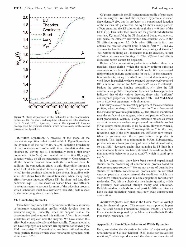
D. Width Dynamics. A measure of the shape of theconcentration profiles is their spatial width. In Figure 9, we showthe dynamics of the half-width, w1/2(t), depicting broadeningof the concentration profile with time. Simulation data areobtained by solving eqs 3.11 numerically from a high orderpolynomial fit to b(r,t). As pointed out in section III, w1/2(t)depends weakly on all the parameters except τ. Consequently,all the theories coincide here with the simulation data. Inaddition, the competition effect is only discernible through asmall kink at intermediate times in panel B. For comparison,w1/2(t) for the geminate solution is also shown. It exhibits onlysmall deviations from the simulation data, when many-bodyeffects become important (Figure 9B). Its short- and long-timebehaviors, eqs 3.12, are shown as dashed lines. Free diffusionin solution seems to account for most of the widening process,which is therefore much less instructive than b(R,t) with respectto the underlying kinetic mechanism.

VI. Concluding Remarks

There have been very little experimental or theoretical studiesof substrate concentration profiles which develop near anactivated enzyme. Evidently, when the enzyme is idle, theconcentration profile around it is uniform. After it is activated,substrates are depleted near the enzyme. We have studied thiseffect both computationally and theoretically. Computationally,we have employed our accurate BD algorithm for studying theMM mechanism.31 Theoretically, we have utilized modernmany-particle theories which show remarkable agreement withsimulations.14,18,21

Of prime interest is the SS concentration profile of substratesnear an enzyme. We find the expected hyperbolic distancedependence,32 R/r, but its prefactor is a complicated functionof the various rate parameters. As eq 3.4 shows, many-particleeffects enter into the SS solution through the sf 0 limit of theDFF, F(0). This factor then enters into the generalized Michaelisconstant, KM, modifying the SS fraction of bound enzyme, css,and hence the effective irreversible rate-constant, kpcss in theSS diffusion equation 3.5. Only when diffusion is fast, oneobtains the reaction control limit in which F(0) ) 1, and KM

assumes its familiar form from basic enzymological kinetics.1

Yet, within the living cell, molecules may be crowded, so thatdiffusion becomes rate limiting.11,12 Then F(0) * 1 and effectsdiscussed herein cannot be neglected.

Before a SS concentration profile is established, there is atransient phase during which the initially uniform substrateconcentration evolves into the final SS profile. We have derived(approximate) analytic expressions for the LT of the concentra-tion profiles, b(r,s), eq 3.3, which were inverted numerically toyield b(r,t). In parallel, we have extended our previously reportedBD simulation routine for MM kinetics31 so as to calculate,besides the enzyme binding probability, c(t), also the fullconcentration profile. Comparison between the two approachesindicated that of the various theories, those with “uniform”convergence properties (particularly MPK2/KT and MM-USA)are in excellent agreement with simulation.

Our study revealed an interesting property of the concentrationprofiles, which undergo a “kinetic transition” as a function ofthe enzyme turnover rate parameter, kp. The effect is manifestednear the surface of the enzyme, where competition effects aremost pronounced. When kp is large, substrate molecules whicharrive at the enzyme surface are processed immediately, so thatb(R,t) decays monotonically to its SS value. However, when kp

is small there is time for “quasi-equilibrium” in the first,reversible step of the MM mechanism. Diffusion now replen-ishes the substrate near the enzyme before the product isreleased. This leads to a minimum in b(R,t). Subsequently,product release allows processing of more substrate molecules,so that b(R,t) decreases again, thus attaining its SS limit in anonmonotonic fashion. We have estimated the condition for thenonmonotonic behavior as kpτ e (λ0τ)2/3, which is valid up toλ0τ ≈ 10.

In low dimensions, there have been several experimentalstudies on the broadening of concentration profiles based onfluorescence spectroscopy.37 We are not aware of quantitativestudies of substrate concentration profiles near an activatedenzyme, particularly under intercellular conditions which mayslow down diffusion and lead to acute competition for substratemolecules. Yet, this is a physically meaningful quantity, whichis presently best accessed through theory and simulation.Reliable modern methods for multiparticle diffusive kineticshave yielded predictions which must now await experimentalverification.

Acknowledgment. S.P. thanks the Golda Meir FellowshipFund for financial support. This research was supported in partby The Israel Science Foundation (grant no. 191/03). The FritzHaber Center is supported by the Minerva Gesellschaft fur dieForschung, Munchen, FRG.

Appendix A: Short-Time Behavior of Width Dynamics

Here, we derive the short-time behavior of wf (t) using theSmoluchowski-Collins-Kimball (SCK) model for irreversiblereactions,32 which reproduces well the short-time dynamics of

Figure 9. Time dependence of the half-width of the concentrationprofile, w1/2(t). The short- and long-time behaviors are calculated fromeqs 3.12a and 3.12b, respectively. Here all the approximate theoriesoverlap, even the geminate solution, which deviates only for the secondparameter set (panel B).

12112 J. Phys. Chem. B, Vol. 112, No. 38, 2008 Park and Agmon

b(r,t) for the MM mechanism. Because G(r,t|R) is a dominatingfactor of the broadening dynamics, one can obtain an essentiallyidentical short-time behavior from more sophisticated theories.Therefore, it suffices to provide that of the SCK model.

For the SCK model with a radiation boundary condition,R(t) ) -κ1[B](R,t) and ∆b(r,t) is given by32

∆b(r, t))-κ1

(κ1 + kD)Rr [erfc(r/R- 1

2√z )-W(r/R- 1

2√z,κ1 + kD

kD

√z)] (A1)

where z ) t/τ and W(x,y) ) exp (2xy + y2) erfc(x + y). Fromeqs 3.11, one can obtain

fwf )erfc(wf - 1

2√z )-W(wf - 1

2√z,κ1 + kD

kD

√z)1-W(0,

κ1 + kD

kD

√z)(A2)

At short times, the numerator and the denominator in theabove equation behave as

erfc(u)-W(u, V√z) ∼ V� zπ

e-u2

u2 [1- 2Vu

√z- 3

u2+O(z2)]

(A3)

1-W(0, V√z) ∼ 2V� zπ[1-V

√πz2

+V24z3+O(z3/2)]

(A4)

where u ) (wf - 1)/(2�z) and V ) 1 + κ1/kD. Substitutingthese into eq A2, one can obtain

fwf ≈exp(-u2)

2u2 [1+V√πz2

+O(z)] (A5)

Taking the t f 0 limit in the left-hand side, wf ≈ 1, and weobtain

2fu2 ≈ exp(-u2) (A6)

This equation can be solved numerically for u. With this constantvalue inserted, eq A5 yields wf (t) - 1 ∝ �z.

Appendix B: Pair Distribution Function

Here, we present the pair distribution functions, FAB(r,s) andFCB(r,s), for the IET, SCRTA, MKP2/KT, and MPK3/MET. Inthese approximate theories, the infinite hierarchy of eqs 2.2 istruncated at the three-particle level. The approximated quantityis an extension of R(t) to the next level of hierarchy

RB(r, t) ≡-κ1FABB(r, R, t)+ κ2FCB(r, t) (B1)

In the SCRTA, MPK2/KT, and MPK3/MET, it is ap-proximated as15,16,18

RB(r, s)) b0R(s)- k1b0∆FAB(r, s)+ k2∆FCB(r, s) (B2)

where the effective rate coefficients, ki, are calculated asdescribed in section II.C. The deviation functions for the pairdistribution functions from their chemical kinetic limits aredefined as

∆FAB(r, t) ≡FAB(r, t)- b0a(t) (B3a)

∆FCB(r, t) ≡FCB(r, t)- b0c(t) (B3b)

They initially satisfy

∆FAB(r, 0))∆FCB(r, 0)) 0 (B4)

Substituting eqs B2 and B3 into the LT of eqs 2.2b and 2.2cone finds that the deviation functions obey the reaction diffusionequations:

(s- Lr)∆FAB(r, s))-k1b0∆FAB(r, s)+

(k2 + kp)∆FCB(r, s)+ R(s)δ(r-R)

4πR2(B5a)

(s- Lr)∆FCB(r, s)) k1b0∆FAB(r, s)- (k2 + kp)∆FCB(r, s)

(B5b)

Note that while these equations are approximate, their sum isthe formally exact eq 3.2.

The solutions of the above equations have the general form:

∆FAB(r, s)

R(s)) µG(r, s|R)+ (1- µ)G(r, sp + λ|R) (B6a)

∆FCB(r, s)

R(s)) (1- µ)[G(r, s|R)- G(r, sp + λ|R)] (B6b)

with µ defined in eq 2.14. The above equations are approximatebut they sum to the formally exact eq 3.3.

For the IET, which is valid only in the low concentrationlimit, µ ) 1. For the SCRTA, MPK2/KT, and MPK3/MET,the effective rate coefficients are calculated as described insection II.C. For the MM-USA, one can obtain ∆FAB(R,s) and∆FCB(R,s) from those for the SCRTA by further replacing thesecond term of the right-hand side in eqs B6 as described insection II.C.

When b(R,t) shows nonmonotonic behavior, one can estimatenumerically the time for the maximum and minimum by solv-ing the equations: dFCB(R,t) ⁄dt ) 0 and FAB(R,t) ) FCB(R,t),respectively. The estimated times become more accurate askp/λ0 decreases (see Figure 7B).

Appendix C: Characteristic Recovery Time of ∆brev(R,t)

As discussed in section V.C, nonmonotonic evolution of b(R,t)occurs when the time scale, tr, for recovery of b(R,t) is smallerthan that for the enzymatic turnover, tp ) 1/kp. Here, we estimatetr under an assumption of time scale separation.

From eqs 2.7, 2.11a, and 3.7a, ∆brev(R,s) at small s can bewritten as

∆brev(R, s) ∼ -κ1

kDtb(1- √τs) (C1)

where the binding time, tb, is defined as

tb ≡ 1/[λ0 + kpF(0)] (C2)

We now assume that due to the separation of time scales wehave

λ0 . kpF(0) (C3)

so that tb is approximated as 1/λ0, see eq 5.1a.Inverting eq C1 into the time domain, we obtain the long-

time behavior of ∆brev(R,t) as

Concentration Profiles near an Activated Enzyme J. Phys. Chem. B, Vol. 112, No. 38, 2008 12113

∆brev(R, t) ∼ -κ1/kD

2√π

tb

τ (τt )3/2

(C4)

This suggests defining a recovery time

tr

τ≡(tb

τ )2/3

(C5)

as given in eq 5.1b. This result was verified numerically.

References and Notes

(1) Fersht, A. Structure and Mechanism in Protein Science: A Guideto Enzyme Catalysis and Protein Folding, 1st ed.; Freeman: New York,1999.

(2) Engasser, J.-M.; Horvath, C. J. Theor. Biol. 1973, 42, 137.(3) Atkins, G. L.; Nimmo, I. A. Biochem. J. 1975, 149, 775.(4) Clark, D. S.; Bailey, J. E. Biotechnol. Bioeng. 1983, 25, 1027.(5) Agmon, N. J. Theor. Biol. 1985, 113, 711.(6) Arrio-Dupont, M.; Bechet, J.-J. Biochimie 1989, 71, 833.(7) Nelsestuen, G. L.; Martinez, M. B. Biochemistry 1997, 36, 9081.(8) Agmon, N. J. Phys. Chem. B 2000, 104, 7830.(9) English, B. P.; Min, W.; van Oijen, A. M.; Lee, K. T.; Luo, G.;

Sun, H.; Cherayil, B. J.; Kou, S. C.; Xie, X. S. Nat. Chem. Biol. 2006, 2,87.

(10) Min, W.; Gopich, I. V.; English, B. P.; Kou, S. C.; Xie, X. S.;Szabo, A. J. Phys. Chem. B 2006, 110, 20093.

(11) Luby-Phelps, K. Int. ReV. Cytol. 2000, 192, 189.(12) Dayel, M. J.; Hom, E. F. Y.; Verkman, A. S. Biophys. J. 1999, 76,

2843.(13) Lee, S.; Karplus, M. J. Chem. Phys. 1987, 86, 1883.

(14) Sung, J.; Lee, S. J. Chem. Phys. 1999, 111, 796.(15) Sung, J.; Lee, S. J. Chem. Phys. 1999, 111, 10159.(16) Sung, J.; Lee, S. J. Chem. Phys. 2000, 112, 2128.(17) Ivanov, K. L.; Lukzen, N. N.; Kipriyanov, A. A.; Doktorov, A. B.

Phys. Chem. Chem. Phys. 2004, 6, 1706.(18) Gopich, I. V.; Szabo, A. J. Chem. Phys. 2002, 117, 507.(19) Yang, M.; Lee, S.; Shin, K. J. J. Chem. Phys. 1998, 108, 117.(20) Yang, M.; Lee, S.; Shin, K. J. J. Chem. Phys. 1998, 108, 8557.(21) Yang, M.; Lee, S.; Shin, K. J. J. Chem. Phys. 1998, 108, 9069.(22) Gopich, I. V.; Doktorov, A. B. J. Chem. Phys. 1996, 105, 2320.(23) Gopich, I. V.; Kipriyanov, A. A.; Doktorov, A. B. J. Chem. Phys.

1999, 110, 10888.(24) Popov, A. V.; Agmon, N. J. Chem. Phys. 2001, 115, 8921.(25) Popov, A. V.; Agmon, N. J. Chem. Phys. 2002, 117, 4376.(26) Popov, A. V.; Agmon, N. J. Chem. Phys. 2003, 118, 11057.(27) Agmon, N.; Popov, A. V. J. Chem. Phys. 2003, 119, 6680.(28) Park, S.; Shin, K. J.; Popov, A. V.; Agmon, N. J. Chem. Phys.

2005, 123, 034507.(29) Zhou, H.-X. J. Phys. Chem. B 1997, 101, 6642.(30) Kim, H.; Yang, M.; Choi, M.-U.; Shin, K. J. J. Chem. Phys. 2001,

115, 1455.(31) Park, S.; Agmon, N. J. Phys. Chem. B 2008, 112, 5977.(32) Rice, S. A. Diffusion-Limited Reactions. Comprehensive Chemical

Kinetics Series; Elsevier: Amsterdam, 1985; Vol. 25.(33) Andre, J. C.; Baros, F.; Winnik, M. A. J. Phys. Chem. 1990, 94,

2942.(34) Agmon, N. Phys. ReV. E 1993, 47, 2415.(35) Edelstein, A. L.; Agmon, N. J. Chem. Phys. 1993, 99, 5396.(36) Gopich, I. V.; Agmon, N. J. Chem. Phys. 1999, 110, 10433.(37) Park, S. H.; Peng, H.; Kopelman, R.; Argyrakis, P.; Taitelbaum,

H. Phys. ReV. E 2006, 73, 041104.

JP803873P

12114 J. Phys. Chem. B, Vol. 112, No. 38, 2008 Park and Agmon