405


P1: OTA/XYZ P2: ABCfm JWBS043-Rogers October 8, 2010 21:3 Printer Name: Yet to Come
CONCISE PHYSICALCHEMISTRY
DONALD W. ROGERSDepartment of Chemistry and BiochemistryThe Brooklyn CenterLong Island UniversityBrooklyn, NY
A JOHN WILEY & SONS, INC., PUBLICATION

P1: OTA/XYZ P2: ABCfm JWBS043-Rogers October 8, 2010 21:3 Printer Name: Yet to Come

P1: OTA/XYZ P2: ABCfm JWBS043-Rogers October 8, 2010 21:3 Printer Name: Yet to Come
CONCISE PHYSICAL CHEMISTRY

P1: OTA/XYZ P2: ABCfm JWBS043-Rogers October 8, 2010 21:3 Printer Name: Yet to Come

P1: OTA/XYZ P2: ABCfm JWBS043-Rogers October 8, 2010 21:3 Printer Name: Yet to Come
CONCISE PHYSICALCHEMISTRY
DONALD W. ROGERSDepartment of Chemistry and BiochemistryThe Brooklyn CenterLong Island UniversityBrooklyn, NY
A JOHN WILEY & SONS, INC., PUBLICATION

P1: OTA/XYZ P2: ABCfm JWBS043-Rogers October 8, 2010 21:3 Printer Name: Yet to Come
Copyright C© 2011 by John Wiley & Sons, Inc. All rights reserved.
Published by John Wiley & Sons, Inc., Hoboken, New Jersey.Published simultaneously in Canada.
No part of this publication may be reproduced, stored in a retrieval system, or transmitted in any form orby any means, electronic, mechanical, photocopying, recording, scanning, or otherwise, except aspermitted under Section 107 or 108 of the 1976 United States Copyright Act, without either the priorwritten permission of the Publisher, or authorization through payment of the appropriate per-copy fee tothe Copyright Clearance Center, Inc., 222 Rosewood Drive, Danvers, MA 01923, (978) 750-8400,fax (978) 750-4470, or on the web at www.copyright.com. Requests to the Publisher for permissionshould be addressed to the Permissions Department, John Wiley & Sons, Inc., 111 River Street, Hoboken,NJ 07030, (201) 748-6011, fax (201) 748-6008, or online at http://www.wiley.com/go/permission.
Limit of Liability/Disclaimer of Warranty: While the publisher and author have used their best efforts inpreparing this book, they make no representations or warranties with respect to the accuracy orcompleteness of the contents of this book and specifically disclaim any implied warranties ofmerchantability or fitness for a particular purpose. No warranty may be created or extended by salesrepresentatives or written sales materials. The advice and strategies contained herein may not be suitablefor your situation. You should consult with a professional where appropriate. Neither the publisher norauthor shall be liable for any loss of profit or any other commercial damages, including but not limited tospecial, incidental, consequential, or other damages.
For general information on our other products and services or for technical support, please contact ourCustomer Care Department within the United States at (800) 762-2974, outside the United States at(317) 572-3993 or fax (317) 572-4002.
Wiley also publishes its books in a variety of electronic formats. Some content that appears in print maynot be available in electronic formats. For more information about Wiley products, visit our web site atwww.wiley.com.
Don Rogers is an amateur jazz musician and painter who lives in Greenwich Village, NY.
Library of Congress Cataloging-in-Publication Data:
Rogers, Donald W.Concise physical chemistry / by Donald W. Rogers.
p. cm.Includes index.Summary: “This book is a physical chemistry textbook that presents the essentials of physical
chemistry as a logical sequence from its most modest beginning to contemporary research topics. Manybooks currently on the market focus on the problem sets with a cursory treatment of the conceptualbackground and theoretical material, whereas this book is concerned only with the conceptualdevelopment of the subject. It contains mathematical background, worked examples and problemsets.Comprised of 21 chapters, the book addresses ideal gas laws, real gases, the thermodynamics of simplesystems, thermochemistry, entropy and the second law, the Gibbs free energy, equilibrium, statisticalapproaches to thermodynamics, the phase rule, chemical kinetics, liquids and solids, solution chemistry,conductivity, electrochemical cells, atomic theory, wave mechanics of simple systems, molecular orbitaltheory, experimental determination of molecular structure, and photochemistry and the theory ofchemical kinetics”– Provided by publisher.
ISBN 978-0-470-52264-6 (pbk.)1. Chemistry, Physical and theoretical–Textbooks. I. Title.
QD453.3.R63 2010541–dc22
2010018380
Printed in Singapore
10 9 8 7 6 5 4 3 2 1
P1: OTA/XYZ P2: ABCfm JWBS043-Rogers October 8, 2010 21:3 Printer Name: Yet to Come
CONTENTS
Foreword xxi
Preface xxiii
1 Ideal Gas Laws 1
1.1 Empirical Gas Laws, 11.1.1 The Combined Gas Law, 21.1.2 Units, 2
1.2 The Mole, 31.3 Equations of State, 41.4 Dalton’s Law, 5
Partial Pressures, 51.5 The Mole Fraction, 61.6 Extensive and Intensive Variables, 61.7 Graham’s Law of Effusion, 6
Molecular Weight Determination, 61.8 The Maxwell–Boltzmann Distribution, 7
Figure 1.1 The Probability Density for Velocities of IdealGas Particles at T �= 0., 8
Boltzmann’s Constant, 8Figure 1.2 A Maxwell–Boltzmann Distribution Over
Discontinuous Energy Levels., 81.9 A Digression on “Space”, 9
Figure 1.3 The Gaussian Probability Density Distributionin 3-Space., 10
The Gaussian Distribution in 2- and 3- and 4-Space, 10
v
P1: OTA/XYZ P2: ABCfm JWBS043-Rogers October 8, 2010 21:3 Printer Name: Yet to Come
vi CONTENTS
1.10 The Sum-Over-States or Partition Function, 10Figure 1.4 The Probability Density of Molecular Velocities
in a Spherical Velocity Space., 12Problems and Exercises, 12
Exercise 1.1, 12Exercise 1.2, 13Problems 1.1–1.13, 15–16Computer Exercise 1.14, 16Problems 1.15–1.18, 16–17
2 Real Gases: Empirical Equations 18
2.1 The van der Waals Equation, 182.2 The Virial Equation: A Parametric Curve Fit, 192.3 The Compressibility Factor, 20
Figure 2.1 A Quadratic Least-Squares Fit to anExperimental Data Set for the Compressibility Factor ofNitrogen at 300 K and Low Pressures (Sigmaplot 11.0 C©)., 21
File 2.1 Partial Output From a Quadratic Least-SquaresCurve Fit to the Compressibility Factor of Nitrogen at300 K (SigmaPlot 11.0 C©)., 22
Figure 2.2 The Second Virial Coefficient of Three Gases asa Function of Temperature., 22
2.3.1 Corresponding States, 23Figure 2.3 The Z = f (p) Curve for Two Different Gases or
for the Same Gas at Two Different Temperatures., 232.4 The Critical Temperature, 24
Figure 2.4 Three Isotherms of a van der Waals Gas., 24Figure 2.5 Conversion of a Liquid to Its Vapor Without
Boiling (1–4)., 252.4.1 Subcritical Fluids, 252.4.2 The Critical Density, 26Figure 2.6 Density ρ Curves for Liquid and Gaseous
Oxygen., 262.5 Reduced Variables, 272.6 The Law of Corresponding States, Another View, 27
Figure 2.7 Compressibility Factors Calculated from thevan der Waals Constants., 28
2.7 Determining the Molar Mass of a Nonideal Gas, 28Problems and Exercises, 28
Exercise 2.1, 28Figure 2.8 Boyle’s Law Plot for an Ideal Gas (lower curve)
and for Nitrogen (upper curve)., 29Exercise 2.2, 30
P1: OTA/XYZ P2: ABCfm JWBS043-Rogers October 8, 2010 21:3 Printer Name: Yet to Come
CONTENTS vii
Table 2.1 Observed Real Gas Behavior from 10 to 100 barExpressed as (p, pVm)., 30
Figure 2.9 Experimental Values of pVm = z(p) vs. p for aReal Gas., 30
Table 2.2 Observed Real Gas Behavior Expressedas (p, pVm)., 31
Figure 2.10 Quadratic Real Gas Behavior., 32Problems 2.1–2.15, 32–34Figure 2.11 Cubic Real Gas Behavior., 34
3 The Thermodynamics of Simple Systems 35
3.1 Conservation Laws and Exact Differentials, 353.1.1 The Reciprocity Relationship, 36
3.2 Thermodynamic Cycles, 37Figure 3.1 Different Path Transformations from A to B., 383.2.1 Hey, Let’s Make a Perpetual Motion Machine!, 38
3.3 Line Integrals in General, 39Figure 3.2 Different Segments of a Curved Rod., 393.3.1 Mathematical Interlude: The Length of an Arc, 40Figure 3.3 Pythagorean Approximation to the Short
Arc of a Curve., 403.3.2 Back to Line Integrals, 41
3.4 Thermodynamic States and Systems, 413.5 State Functions, 413.6 Reversible Processes and Path Independence, 42
Figure 3.4 The Energy Change for Reversible Expansion ofan Ideal Gas., 43
3.7 Heat Capacity, 443.8 Energy and Enthalpy, 443.9 The Joule and Joule–Thomson Experiments, 46
Figure 3.5 Inversion Temperature Ti as a Function ofPressure., 47
3.10 The Heat Capacity of an Ideal Gas, 48Table 3.1 Heat Capacities and γ for Selected Gases., 48Figure 3.6. Typical Heat Capacity as a Function of
Temperature for a Simple Organic Molecule., 503.11 Adiabatic Work, 50
Figure 3.7 Two Expansions of an Ideal Gas., 51Problems and Example, 52
Example 3.1, 52Problems 3.1–3.12, 52–55Figure 3.8 C = Diagonal Along x = 1 to y = 1., 53Figure 3.9 C = Quarter-Circular Arc., 53
P1: OTA/XYZ P2: ABCfm JWBS043-Rogers October 8, 2010 21:3 Printer Name: Yet to Come
viii CONTENTS
4 Thermochemistry 56
4.1 Calorimetry, 564.2 Energies and Enthalpies of Formation, 574.3 Standard States, 584.4 Molecular Enthalpies of Formation, 58
Figure 4.1 Combustion of C(gr) and CO(g)., 59Figure 4.2 A Thermochemical Cycle for Determining
� f H 298(methane)., 604.5 Enthalpies of Reaction, 604.6 Group Additivity, 624.7 � f H 298(g) from Classical Mechanics, 644.8 The Schrodinger Equation, 644.9 Variation of �H with T, 654.10 Differential Scanning Calorimetry, 66
Figure 4.3 Schematic Diagram of the Thermal Denaturationof a Water-Soluble Protein., 67
Problems and Example, 68Example 4.1, 68Problems 4.1–4.9, 68–70
5 Entropy and the Second Law 71
5.1 Entropy, 71Figure 5.1 An Engine., 725.1.1 Heat Death and Time’s Arrow, 735.1.2 The Reaction Coordinate, 735.1.3 Disorder, 74
5.2 Entropy Changes, 745.2.1 Heating, 745.2.2 Expansion, 755.2.3 Heating and Expansion, 75
5.3 Spontaneous Processes, 775.3.1 Mixing, 775.3.2 Heat Transfer, 775.3.3 Chemical Reactions, 78
5.4 The Third Law, 785.4.1 Chemical Reactions (Again), 79
Problems and Example, 80Example 5.1, 80Figure 5.2 C p/T vs. T for Metallic Silver Ag(s)., 81Problems 5.1–5.9, 81–83
6 The Gibbs Free Energy 84
6.1 Combining Enthalpy and Entropy, 846.2 Free Energies of Formation, 85
P1: OTA/XYZ P2: ABCfm JWBS043-Rogers October 8, 2010 21:3 Printer Name: Yet to Come
CONTENTS ix
6.3 Some Fundamental Thermodynamic Identities, 866.4 The Free Energy of Reaction, 876.5 Pressure Dependence of the Chemical Potential, 87
Figure 6.1 A Reaction Diagram for �G4., 886.5.1 The Equilibrium Constant as a Quotient of Quotients, 88
6.6 The Temperature Dependence of the Free Energy, 88Problems and Example, 90
Example 6.1, 90Problems 6.1–6.12, 90–92
7 Equilibrium 93
7.1 The Equilibrium Constant, 937.2 General Formulation, 947.3 The Extent of Reaction, 967.4 Fugacity and Activity, 977.5 Variation of the Equilibrium Constant with Temperature, 97
The van’t Hoff Equation, 987.5.1 Le Chatelier’s Principle, 997.5.2 Entropy from the van’t Hoff Equation, 99
7.6 Computational Thermochemistry, 1007.7 Chemical Potential: Nonideal Systems, 1007.8 Free Energy and Equilibria in Biochemical Systems, 102
7.8.1 Making ATP, the Cell’s Power Supply, 103Problems and Examples, 104
Example 7.1, 104Example 7.2, 105Problems 7.1–7.7, 105–106
8 A Statistical Approach to Thermodynamics 108
8.1 Equilibrium, 108Figure 8.1 A Two-Level Equilibrium., 109Figure 8.2 A Two-Level Equilibrium., 109
8.2 Degeneracy and Equilibrium, 109Figure 8.3 A Degenerate Two-Level Equilibrium., 110Figure 8.4 A Degenerate Two-Level Equilibrium., 110Figure 8.5 A Two-Level Equilibrium with Many A and
Many B Levels., 1118.3 Gibbs Free Energy and the Partition Function, 1128.4 Entropy and Probability, 1138.5 The Thermodynamic Functions, 113
Table 8.1 Thermodynamic Functions (Irikura, 1998)., 1148.6 The Partition Function of a Simple System, 1148.7 The Partition Function for Different Modes of Motion, 116
P1: OTA/XYZ P2: ABCfm JWBS043-Rogers October 8, 2010 21:3 Printer Name: Yet to Come
x CONTENTS
8.8 The Equilibrium Constant: A Statistical Approach, 1178.9 Computational Statistical Thermodynamics, 119
Table 8.2 Some Computed Partition Functions forMolecular and Atomic Sodium., 120
Problems and Examples, 120Example 8.1, 120Example 8.2, 121Problems 8.1–8.9, 122–123
9 The Phase Rule 124
9.1 Components, Phases, and Degrees of Freedom, 1249.2 Coexistence Curves, 125
Figure 9.1 Pure Water in One Phase (left) and Two Phases(right)., 126
Figure 9.2 A Liquid–Vapor Coexistence Curve., 127Figure 9.3 A Single-Component Phase Diagram., 128
9.3 The Clausius–Clapeyron Equation, 1289.4 Partial Molar Volume, 129
Figure 9.4 Total Volume of an Ideal Binary Solution., 130Figure 9.5 Volume Increase (or Decrease) Upon Adding
Small Amounts of Solute n2 to Pure Solvent., 1309.4.1 Generalization, 130Figure 9.6 Partial Molar Volume as the Slope of
V vs. n2., 131Figure 9.7 Volume Behavior of a Nonideal Binary
Solution., 1319.5 The Gibbs Phase Rule, 1349.6 Two-Component Phase Diagrams, 134
9.6.1 Type 1, 135Figure 9.8 A Type I Phase Diagram., 1359.6.2 Type II, 136Figure 9.9 A Type II Phase Diagram., 1359.6.3 Type III, 137Figure 9.10 A Type III Phase Diagram., 137
9.7 Compound Phase Diagrams, 137Figure 9.11 A Compound Phase Diagram with a Low
Boiling Azeotrope., 1389.8 Ternary Phase Diagrams, 138
Figure 9.12 A Ternary Phase Diagram with a Tie Line., 139Problems and Examples, 139
Example 9.1, 139Figure 9.13 The Liquid–Vapor Coexistence Curve of Water
Leading to �vap H (H2O) = 44.90kJmol−1., 140
P1: OTA/XYZ P2: ABCfm JWBS043-Rogers October 8, 2010 21:3 Printer Name: Yet to Come
CONTENTS xi
Example 9.2, 140Figure 9.14 A Ternary Phase Diagram in which B and C Are
Partially Miscible., 141Problems 9.1–9.9, 141–143
10 Chemical Kinetics 144
10.1 First-Order Kinetic Rate Laws, 144Figure 10.1 First-Order Radioactive Decay., 146Figure 10.2 Logarithmic Decay of a Radioactive Element., 147
10.2 Second-Order Reactions, 14710.3 Other Reaction Orders, 149
10.3.1 Mathematical Interlude: The Laplace Transform, 14910.3.2 Back to Kinetics: Sequential Reactions, 15010.3.3 Reversible Reactions, 151
10.4 Experimental Determination of the Rate Equation, 15410.5 Reaction Mechanisms, 15410.6 The Influence of Temperature on Rate, 156
Figure 10.3 An Activation Energy Barrier Between anUnstable Position and a Stable Position., 156
Figure 10.4 Enthalpy Level Diagram for an ActivatedComplex [B]., 157
Figure 10.5 An Activation Barrier., 157Figure 10.6 A Boltzmann Distribution of Molecular Speeds., 158
10.7 Collision Theory, 15810.8 Computational Kinetics, 159Problems and Examples, 160
Example 10.1, 160Example 10.2, 160Figure 10.7 First-Order Fluorescence Decline from
Electronically Excited Iodine in Milliseconds., 161Figure 10.8 The Natural Logarithm of Relative Intensity vs.
Time for Radiative Decay., 161Problems 10.1–10.10, 162–164
11 Liquids and Solids 165
11.1 Surface tension, 165Figure 11.1 Intermolecular Attractive Forces Acting Upon
Molecules at an Air–Water Interface., 166Figure 11.2 Stretching a Two-Dimensional Membrane by
Moving an Edge of Length l., 166Figure 11.3 Stretching a Two-Dimensional Liquid
Bimembrane., 167Figure 11.4 Capillary Rise in a Tube of Radius R., 167
P1: OTA/XYZ P2: ABCfm JWBS043-Rogers October 8, 2010 21:3 Printer Name: Yet to Come
xii CONTENTS
11.2 Heat Capacity of Liquids and Solids, 168Figure 11.5 Heat Capacity as a Function of Temperature., 168
11.3 Viscosity of Liquids, 169Figure 11.6 Approximation of Laminar Flow Inside a Tube., 169
11.4 Crystals, 170Figure 11.7 Close Packing of Marbles Between Two Sheets., 171Figure 11.8 A Less Efficient Packing of Marbles., 172Figure 11.9 Bragg’s Law for Constructive Reflection., 17311.4.1 X-Ray Diffraction: Determination of Interplanar
Distances, 173Figure 11.10 A Face-Centered Cubic Unit Cell., 17411.4.2 The Packing Fraction, 174Figure 11.11 A Two-Dimensional Unit Cell for
Packing of Discs., 175Figure 11.12 A Simple Cubic Cell., 175
11.5 Bravais Lattices, 176Table 11.1 The Bravais Crystal Systems and Lattices., 17611.5.1 Covalent Bond Radii, 176
11.6 Computational Geometries, 17711.7 Lattice Energies, 177Problems and Exercise, 178
Exercise 11.1, 178Figure 11.13 The Born–Haber Cycle for NaI., 179Problems 11.1–11.8, 179–181Figure 11.14 Close Packing (left) and Simple Square Unit
Cells (right)., 180Figure 11.15 A Body-Centered Primitive Cubic Cell., 180
12 Solution Chemistry 182
12.1 The Ideal Solution, 182Figure 12.1 Entropy, Enthalpy, and Gibbs Free Energy
Changes for Ideal Mixing at T > 0., 18312.2 Raoult’s Law, 183
Figure 12.2 Partial and Total Pressures for a Raoult’sLaw Solution., 184
12.3 A Digression on Concentration Units, 18412.4 Real Solutions, 185
Figure 12.3 Consistent Positive Deviations fromRaoult’s Law., 185
12.5 Henry’s Law, 186Figure 12.4 Henry’s Law for the Partial Pressure of
Component B as the Solute., 18612.5.1 Henry’s Law Activities, 186
P1: OTA/XYZ P2: ABCfm JWBS043-Rogers October 8, 2010 21:3 Printer Name: Yet to Come
CONTENTS xiii
12.6 Vapor Pressure, 18712.7 Boiling Point Elevation, 188
Figure 12.5 Boiling of Pure Solvent (left) and a Solution ofSolvent and Nonvolatile Solute (right)., 189
12.8 Osmotic Presure, 191Figure 12.6 Osmotic Pressure, π ., 192
12.9 Colligative Properties, 194Figure 12.7 Lowering of the Freezing Point of Water
by Ammonia., 195Problems, Examples, and Exercise, 195
Example 12.1, 195Table 12.1 Vapor Pressures of Acetone over Dilute Binary
Solutions of Acetone in Diethyl Ether., 196Example 12.2, 196Exercise 12.1, 198Exercise 12.2, 199Problems 12.1–12.10, 199–202
13 Coulometry and Conductivity 203
13.1 Electrical Potential, 20313.1.1 Membrane Potentials, 203Figure 13.1 The Potential Drop Between Charged Plates
Is V = φ(0) − φ(l)., 204Figure 13.2 An Ion-Permeable Membrane (Schematic)., 204
13.2 Resistivity, Conductivity, and Conductance, 20513.3 Molar Conductivity, 206
Figure 13.3 Kohlrausch’s Law for Conductance of theStrong Electrolytes HCl and NaOAc and the WeakElectrolyte HOAc., 207
13.4 Partial Ionization: Weak Electrolytes, 20813.5 Ion Mobilities, 209
Figure 13.4 Moving Boundary Determination of theMobility of H+., 210
13.6 Faraday’s Laws, 21113.7 Mobility and Conductance, 21113.8 The Hittorf Cell, 211
Figure 13.5 A Three-Compartment Hittorf Cell., 21213.9 Ion Activities, 213Problems and Examples, 215
Example 13.1, 215Example 13.2, 216Example 13.3, 216Problems 13.1–13.11, 217–219

P1: OTA/XYZ P2: ABCfm JWBS043-Rogers October 8, 2010 21:3 Printer Name: Yet to Come
xiv CONTENTS
14 Electrochemical Cells 220
14.1 The Daniell Cell, 22014.2 Half-Cells, 221
Figure 14.1 The Hydrogen Half-Cell., 22214.3 Half-Cell Potentials, 222
Table 14.1 A Few Selected Reduction Potentials., 22314.4 Cell Diagrams, 22314.5 Electrical Work, 22414.6 The Nernst Equation, 22414.7 Concentration Cells, 22514.8 Finding E◦, 226
Figure 14.2 Extrapolation to E◦ = 0.2223 for theStandard Hydrogen–Silver–Silver ChlorideCell., 228
14.9 Solubility and Stability Products, 22814.10 Mean Ionic Activity Coefficients, 22914.11 The Calomel Electrode, 22914.12 The Glass Electrode, 230
Problems and Examples, 230Example 14.1, 230Example 14.2, 231Figure 14.3 The Mean Activity Coefficient of HCl as a
Function of m1/2., 232Problems 14.1–14.9, 232–234
15 Early Quantum Theory: A Summary 235
15.1 The Hydrogen Spectrum, 235Figure 15.1 The Hydrogen Emission Spectrum., 236Figure 15.2 The First Six Solutions of the H Atom Energy
Calculated by Bohr (1913)., 23615.2 Early Quantum Theory, 236
Schrodinger, Heisenberg, and Born: An Introduction, 237The Hamiltonian Operator, 237
15.3 Molecular Quantum Chemistry, 238Heitler and London, 238Hartree and Fock, 239Antisymmetry and Determinantal Wave Functions, 240
15.4 The Hartree Independent Electron Method, 24015.5 A Digression on Atomic Units, 243
Problems and Examples, 243Example 15.1, 243Example 15.2, 244Problems 15.1–15.9, 246–247
P1: OTA/XYZ P2: ABCfm JWBS043-Rogers October 8, 2010 21:3 Printer Name: Yet to Come
CONTENTS xv
16 Wave Mechanics of Simple Systems 248
16.1 Wave Motion, 248Figure 16.1 Graph of sin(x), sin(2x), and sin(3x) Shown
over the Interval 0, π ., 24916.2 Wave equations, 249
Eigenvalues and Eigenvectors, 25016.3 The Schrodinger Equation, 25016.4 Quantum Mechanical Systems, 251
� is a Vector, 251The Eigenfunction Postulate, 252
16.5 The Particle in a One-Dimensional Box, 253Figure 16.2 Wave Forms for the First Three Wave
Functions of the Particle in a Box., 254Fundamentals and Overtones, 254Figure 16.3 A Mathcad C© Sketch of the Born Probability
Densities at the First Three Levels of the Particle ina Box., 255
16.6 The Particle in a Cubic Box, 255Separable Equations, 25616.6.1 Orbitals, 257Figure 16.4 The Ground State Orbital of a
Particle Confined to a Cubic Box., 25716.6.2 Degeneracy, 257Figure 16.5 The First Excited State of a Particle
Confined to a Cubic Box., 25716.6.3 Normalization, 257Figure 16.6 The Degenerate Energy Levels for
the Hydrogen Atom., 25816.7 The Hydrogen Atom, 258
The Radial Equation and Probability “Shells”, 25816.8 Breaking Degeneracy, 259
Figure 16.7 Reduced Degeneracy in Energy Levels forHydrogen-Like Atoms., 260
16.8.1 Higher Exact Solutions for the Hydrogen Atom, 260Table 16.1 The First Six Wave Functions for Hydrogen., 261Table 16.2 The First Three s Wave Functions for
Hydrogen (Simplified Form)., 261Figure 16.8 Roots of the Radial 3s Wave Function of
Atomic Hydrogen as a Function of Distance r ., 261Figure 16.9 The Radial Probability Density for
an Electron in the 3s Orbital of Hydrogen., 26216.9 Orthogonality and Overlap, 262
Figure 16.10 The Radial Node of the 2p AtomicOrbital., 262
P1: OTA/XYZ P2: ABCfm JWBS043-Rogers October 8, 2010 21:3 Printer Name: Yet to Come
xvi CONTENTS
Figure 16.11 Favorable spx and Unfavorable spz
Overlap of Orbitals Depending upon OrbitalSymmetry., 263
16.10 Many-Electron Atomic Systems, 263The Hartree Method, 263
Problems 16.1–16.9, 264–266
17 The Variational Method: Atoms 267
17.1 More on the Variational Method, 26717.2 The Secular Determinant, 26817.3 A Variational Treatment for the Hydrogen Atom: The
Energy Spectrum, 27117.3.1 Optimizing the Gaussian Function, 272Simultaneous Minima, 272The Exact Wave Function, 272The Gaussian Approximation, 27217.3.2 A GAUSSIAN C© HF Calculation of Eatom:
Computer Files, 273File 17.1 Gaussian gen Input for the Hydrogen Atom., 273File 17.2 Energies Drawn from the Gaussiangen Output File for the Hydrogen Atom., 273
17.4 Helium, 27417.4.1 An SCF Variational Ionization Potential for
Helium, 27517.5 Spin, 27817.6 Bosons and Fermions, 27817.7 Slater Determinants, 27917.8 The Aufbau Principle, 28017.9 The SCF Energies of First-Row Atoms and Ions, 281
Figure 17.1 Calculated IP1 for Elements 1–10., 28117.10 Slater-Type Orbitals (STO), 282
Table 17.1 Slater’s Rules., 28217.11 Spin–Orbit Coupling, 283
Figure 17.2 Linear and Angular Momentum Vectors., 283Problems and Examples, 283
Example 17.1, 283File 17.3 Mathcad C© Calculation of the Ionization
Potential of Helium., 284Example 17.2, 284Problems 17.1–17.9, 285–286
18 Experimental Determination of Molecular Structure 287
18.1 The Harmonic Oscillator, 287Figure 18.1 A Classical Harmonic Oscillator., 288
P1: OTA/XYZ P2: ABCfm JWBS043-Rogers October 8, 2010 21:3 Printer Name: Yet to Come
CONTENTS xvii
18.2 The Hooke’s Law Potential Well, 289Figure 18.2 Parabolic Potential Wells for the Harmonic
Oscillator., 29018.3 Diatomic Molecules, 29018.4 The Quantum Rigid Rotor, 290
Figure 18.3 Energy Levels within a Simple Rotor., 29118.5 Microwave Spectroscopy: Bond Strength and Bond
Length, 29218.6 Electronic Spectra, 292
Figure 18.4 Electronic Promotion in Alkenes., 293Figure 18.5 Absorption Wavelengths of Conjugated
Polyalkenes., 29318.7 Dipole Moments, 294
Figure 18.6 A Charged Parallel Plate Capacitor., 294Figure 18.7 A Charged Capacitor with a Dielectric., 294Dielectric Constant, 294Polarizability, 29518.7.1 Bond Moments, 296Figure 18.8 The Total Dipoles of Two
Dichloroethene Isomers., 29618.8 Nuclear Magnetic Resonance (NMR), 297
18.8.1 Spin–Spin Coupling, 298Figure 18.9 Schematic NMR Spectrum of
Ethanol, CH3CH2OH., 299Magnetic Resonance Imaging (MRI), 299
18.9 Electron Spin Resonance, 299Problems and Examples, 299
Example 18.1, 299Figure 18.10 Schematic Diagram of a Vibration–Rotation
Band., 300Example 18.2, 301Problems 18.1–18.13, 301–304Figure 18.11 The Vibration–Rotation Spectrum of CO., 302
19 Classical Molecular Modeling 305
19.1 Enthalpy: Additive Methods, 305Figure 19.1 Enthalpies of Formation of “Adjacent”
n-Alkanes., 306Group Additivity, 306
19.2 Bond Enthalpies, 306Bond Additivity, 306Figure 19.2 Bond Enthalpies Calculated in CH2, from the
Reference State of Gaseous Atoms (top), and Relativeto Elements in their Standard State (H2(g) and
C(graphite))., 307
P1: OTA/XYZ P2: ABCfm JWBS043-Rogers October 8, 2010 21:3 Printer Name: Yet to Come
xviii CONTENTS
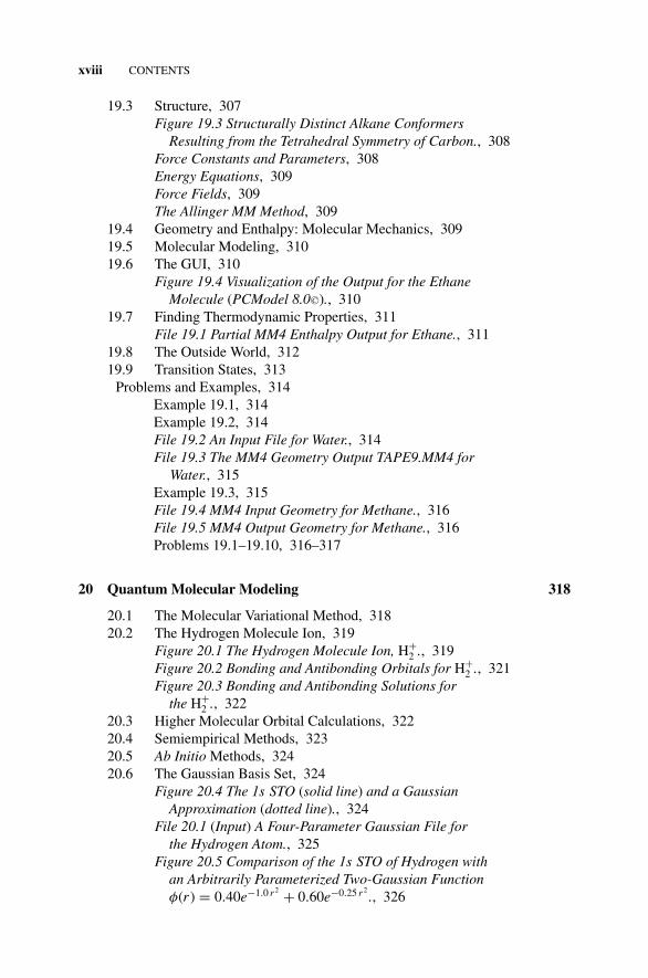
19.3 Structure, 307Figure 19.3 Structurally Distinct Alkane Conformers
Resulting from the Tetrahedral Symmetry of Carbon., 308Force Constants and Parameters, 308Energy Equations, 309Force Fields, 309The Allinger MM Method, 309
19.4 Geometry and Enthalpy: Molecular Mechanics, 30919.5 Molecular Modeling, 31019.6 The GUI, 310
Figure 19.4 Visualization of the Output for the EthaneMolecule (PCModel 8.0 C©)., 310
19.7 Finding Thermodynamic Properties, 311File 19.1 Partial MM4 Enthalpy Output for Ethane., 311
19.8 The Outside World, 31219.9 Transition States, 313
Problems and Examples, 314Example 19.1, 314Example 19.2, 314File 19.2 An Input File for Water., 314File 19.3 The MM4 Geometry Output TAPE9.MM4 for
Water., 315Example 19.3, 315File 19.4 MM4 Input Geometry for Methane., 316File 19.5 MM4 Output Geometry for Methane., 316Problems 19.1–19.10, 316–317
20 Quantum Molecular Modeling 318
20.1 The Molecular Variational Method, 31820.2 The Hydrogen Molecule Ion, 319
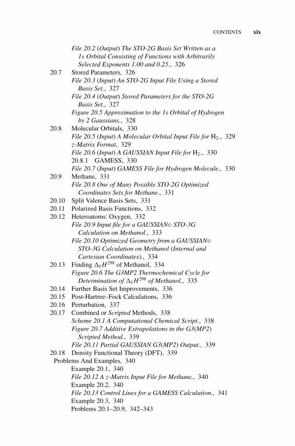
Figure 20.1 The Hydrogen Molecule Ion, H+2 ., 319
Figure 20.2 Bonding and Antibonding Orbitals for H+2 ., 321
Figure 20.3 Bonding and Antibonding Solutions forthe H+
2 ., 32220.3 Higher Molecular Orbital Calculations, 32220.4 Semiempirical Methods, 32320.5 Ab Initio Methods, 32420.6 The Gaussian Basis Set, 324
Figure 20.4 The 1s STO (solid line) and a GaussianApproximation (dotted line)., 324
File 20.1 (Input) A Four-Parameter Gaussian File forthe Hydrogen Atom., 325
Figure 20.5 Comparison of the 1s STO of Hydrogen withan Arbitrarily Parameterized Two-Gaussian Functionφ(r ) = 0.40e−1.0 r2 + 0.60e−0.25 r2
., 326
P1: OTA/XYZ P2: ABCfm JWBS043-Rogers October 8, 2010 21:3 Printer Name: Yet to Come
CONTENTS xix
File 20.2 (Output) The STO-2G Basis Set Written as a1s Orbital Consisting of Functions with ArbitrarilySelected Exponents 1.00 and 0.25., 326
20.7 Stored Parameters, 326File 20.3 (Input) An STO-2G Input File Using a Stored
Basis Set., 327File 20.4 (Output) Stored Parameters for the STO-2G
Basis Set., 327Figure 20.5 Approximation to the 1s Orbital of Hydrogen
by 2 Gaussians., 32820.8 Molecular Orbitals, 330
File 20.5 (Input) A Molecular Orbital Input File for H2., 329z-Matrix Format, 329File 20.6 (Input) A GAUSSIAN Input File for H2., 33020.8.1 GAMESS, 330File 20.7 (Input) GAMESS File for Hydrogen Molecule., 330
20.9 Methane, 331File 20.8 One of Many Possible STO-2G Optimized
Coordinates Sets for Methane., 33120.10 Split Valence Basis Sets, 33120.11 Polarized Basis Functions, 33220.12 Heteroatoms: Oxygen, 332
File 20.9 Input file for a GAUSSIAN C© STO-3GCalculation on Methanol., 333
File 20.10 Optimized Geometry from a GAUSSIAN C©STO-3G Calculation on Methanol (Internal andCartesian Coordinates)., 334
20.13 Finding �f H 298 of Methanol, 334Figure 20.6 The G3MP2 Thermochemical Cycle for
Determination of �f H 298 of Methanol., 33520.14 Further Basis Set Improvements, 33620.15 Post-Hartree–Fock Calculations, 33620.16 Perturbation, 33720.17 Combined or Scripted Methods, 338
Scheme 20.1 A Computational Chemical Script., 338Figure 20.7 Additive Extrapolations in the G3(MP2)
Scripted Method., 339File 20.11 Partial GAUSSIAN G3(MP2) Output., 339
20.18 Density Functional Theory (DFT), 339Problems And Examples, 340
Example 20.1, 340File 20.12 A z-Matrix Input File for Methane., 340Example 20.2, 340File 20.13 Control Lines for a GAMESS Calculation., 341Example 20.3, 340Problems 20.1–20.9, 342–343
P1: OTA/XYZ P2: ABCfm JWBS043-Rogers October 8, 2010 21:3 Printer Name: Yet to Come
xx CONTENTS
21 Photochemistry and the Theory of Chemical Reactions 344
21.1 Einstein’s Law, 34421.2 Quantum Yields, 345
Table 21.1 Some Experimental Quantum Yields., 345Figure 21.1 Mechanism for Fluorescent and
Phosphorescent Light Emission., 34621.2.1 Lipid Peroxidation, 34621.2.2 Ozone Depletion, 347
21.3 Bond Dissociation Energies (BDE), 34821.4 Lasers, 34821.5 Isodesmic Reactions, 34921.6 The Eyring Theory of Reaction Rates, 34921.7 The Potential Energy Surface, 350
Figure 21.2 Eyring Potential Energy Plot for theReaction H + H–H → H–H + H., 350
Figure 21.3 Activation of the Symmetrical ReactionH + H–H → H–H + H., 351
Figure 21.4 The Enthalpy of Activation of an ExothermicReaction., 351
21.7.1 Optical Inversion, 352Figure 21.5 An Optically Active Species., 352Figure 21.6 Inversion of Optical Activity., 352
21.8 The Steady-State Pseudo-Equilibrium, 35321.9 Entropies of Activation, 35421.10 The Structure of the Activated Complex, 355
Problems and Examples, 355Example 21.1, 355Example 21.2, 356Problems 21.1–21.8, 357–359
References 361
Answers to Selected Odd-Numbered Problems 365
Index 369

P1: OTA/XYZ P2: ABCfm JWBS043-Rogers October 8, 2010 21:3 Printer Name: Yet to Come
FOREWORD
Among many advantages of being a professional researcher and teacher is the pleasureof reading a new and good textbook that concisely summarizes the fundamentals andprogress in your research area. This reading not only gives you the enjoyment oflooking once more at the whole picture of the edifice that many generations ofyour colleagues have meticulously build but, most importantly, also enhances yourconfidence that your choice to spend your entire life to promote and contribute tothis structure is worthwhile. Clearly, the perception of the textbook by an expert inthe field is quite different, to say the least, from the perception of a junior or seniorundergraduate student who is about to register for a class. A simple look at a textbookthat is jam-packed with complex integrals and differential equations may scare anyprospective students to death. On the other hand, eliminating the mathematics entirelywill inevitably eliminate the rigor of scientific statements. In this respect, the rightcompromise between simplicity and rigor in explaining complex scientific topics isan extremely rare talent. The task is especially large given the fact that the textbook isaddressed to students for whom a particular area of science is not among their primaryinterests. In this respect, Professor Rogers’s Concise Physical Chemistry is a textbookthat ideally suits all of the above-formulated criteria of a new and good textbook.
Although the fundamental laws and basic principles of physical chemistry wereformulated long ago, research in the area is continuously widening and deepening. Asa result, the original boundaries of physical chemistry as a science become more andmore vague and difficult to determine. During the last two decades, physical chemistryhas made a tremendous progress mainly boosted by a spectacular increase in ourcomputational capabilities. This is especially visible in quantum molecular modeling.For instance, on my first acquaintance with physical chemistry about 30 years ago,the only molecule that could be quantitatively treated with an accuracy close to
xxi
P1: OTA/XYZ P2: ABCfm JWBS043-Rogers October 8, 2010 21:3 Printer Name: Yet to Come
xxii FOREWORD
experimental data by wave mechanics was the hydrogen molecule. In a lifetime, Ihave witnessed a complete change of the research picture in which thermodynamicand kinetic data are theoretically obtained routinely with an accuracy often exceedingthe experimental one. Quite obviously, to keep the pace with the progress in research,textbooks should be permanently updated and revised. In his textbook ProfessorRogers sticks to the classical topics that are conventionally considered as part ofphysical chemistry. However, these classical topics are deciphered from a modernpoint of view, and here lies the main strength of this textbook as well as what actuallymakes this textbook different from many other similar textbooks.
Traditionally, physical chemistry is viewed as an application of physical principlesin explaining and rationalizing chemical phenomena. As such, the powerful principlesand theories that physical chemistry borrows from physics are accompanied by anadvanced and mandatory set of mathematical tools. This makes the process of learningphysical chemistry very difficult albeit challenging, exciting, and rewarding. The levelof mathematics used by Professor Rogers to formulate and prove the physicochemicalprinciples is remarkably consistent throughout the whole text. Thus, only the mostgeneral algebra and calculus concepts are required to understand the essence ofthe topics discussed. Professor Rogers’s way of reasoning is succinct and easy tofollow while the examples used to illustrate the theoretical developments are carefullyselected and always make a good point. There is no doubt that this textbook is a workof great value, and I heartily recommend it for everybody who wants to enter thewonderful world of physical chemistry.
Ilie FishtikWorcester Polytechnic InstituteWorcester, MAJuly 2010
P1: OTA/XYZ P2: ABCfm JWBS043-Rogers October 8, 2010 21:3 Printer Name: Yet to Come
PREFACE
Shall I call that wise or foolish, now; if it be really wise it has a foolish look to it; yet, ifit be really foolish, then has it a sort of wiseish look to it.
Moby-Dick (Chapter 99) —Herman Melville
Physical chemistry stands at the intersection of the power and generality of classicaland quantum physics with the minute molecular complexity of chemistry and biology.Any molecular process that can be envisioned as a flow from a higher energy stateto a lower state is subject to analysis by the methods of classical thermodynamics.Chemical thermodynamics tells us where a process is going. Chemical kinetics tellsus how long it will take to get there.
Evidence for and application of many of the most subtle and abstract principlesof quantum mechanics are to be found in the physical interpretation of chemicalphenomena. The vast expansion of spectroscopy from line spectra of atoms wellknown in the nineteenth century to the magnetic resonance imaging (MRI) of today’sdiagnostic procedures is a result of our gradually enhanced understanding of thequantum mechanical interactions of energy with simple atomic or complex molecularsystems.
Mathematical methods developed in the domain of physical chemistry can besuccessfully applied to very different phenomena. In the study of seemingly unrelatedphenomena, we are astonished to find that electrical potential across a capacitor, therate of isomerization of cyclopentene, and the growth of marine larvae either asindividuals or as populations have been successfully modeled by the same first-orderdifferential equation.
Many people in diverse fields use physical chemistry but do not have the op-portunity to take a rigorous three-semester course or to master one of the several∼1000-page texts in this large and diverse field. Concise Physical Chemistry is
xxiii
P1: OTA/XYZ P2: ABCfm JWBS043-Rogers October 8, 2010 21:3 Printer Name: Yet to Come
xxiv PREFACE
intended to meet (a) the needs of professionals in fields other than physical chemistrywho need to be able to master or review a limited portion of physical chemistry or(b) the need of instructors who require a manageable text for teaching a one-semestercourse in the essentials of the subject. The present text is not, however, a dilutedform of physical chemistry. Topics are treated as brief, self-contained units, gradedin difficulty from a reintroduction to some of the concepts of general chemistry inthe first few chapters to research-level computer applications in the later chapters.
I wish to acknowledge my obligations to Anita Lekhwani and Rebekah Amosof John Wiley and Sons, Inc. and to Tony Li of Scientific Computing, Long IslandUniversity. I also thank the National Center for Supercomputing Applications andthe National Science Foundation for generous allocations of computer time, and theH. R. Whiteley Foundation of the University of Washington for summer researchfellowships during which part of this book was written.
Finally, though many people have helped me in my attempts to better appreciatethe beauty of this vast and variegated subject, this book is dedicated to the memoryof my first teacher of physical chemistry, Walter Kauzmann.
Donald W. Rogers
P1: OTA/XYZ P2: ABCc01 JWBS043-Rogers September 13, 2010 11:20 Printer Name: Yet to Come
1IDEAL GAS LAWS
In the seventeenth and eighteenth centuries, thoughtful people, influenced by thesuccess of early scientists like Galileo and Newton in the fields of mechanics andastronomy, began to look more carefully for quantitative connections among thephenomena around them. Among these people were the chemist Robert Boyle andthe famous French balloonist Jacques Alexandre Cesar Charles.
1.1 EMPIRICAL GAS LAWS
Many physical chemistry textbooks begin, quite properly, with a statement of Boyle’sand Charles’s laws of ideal gases:
pV = k1 (Boyle, 1662)
and
V = k2T (Charles, 1787)
The constants k1 and k2 can be approximated simply by averaging a series of experi-mental measurements, first of pV at constant temperature T for the Boyle equation,then of V/T at constant pressure p for Charles’s law. All this can be done using simplemanometers and thermometers.
Concise Physical Chemistry, by Donald W. RogersCopyright C© 2011 John Wiley & Sons, Inc.
1
P1: OTA/XYZ P2: ABCc01 JWBS043-Rogers September 13, 2010 11:20 Printer Name: Yet to Come
2 IDEAL GAS LAWS
1.1.1 The Combined Gas Law
These two laws can be combined to give a new constant
pV
T= k3
Subsequently, it was found that if the quantity of gas taken is the number of gramsequal to the atomic or molecular weight of the gas, the constant k3, now written Runder the new stipulations, is given by
pV = RT
For the number of moles of a gas, n, we have
pV = n RT
The constant R is called the universal gas constant.
1.1.2 Units
The pressure of a confined gas is the sum of the force exerted by all of the gasmolecules as they impact with the container walls of area A in unit time:
p = f in units of N
A in units of m2
The summed force f is given in units of newtons (N), and the area is in square meters(m2). The N m−2 is also called the pascal (Pa). The pascal is about five or six ordersof magnitude smaller than pressures encountered in normal laboratory practice, sothe convenient unit 1 bar ≡ 105 Pa was defined.
The logical unit of volume in the MKS (meter, kilogram, second) system is them3, but this also is not commensurate with routine laboratory practice where the literis used. One thousand liters equals 1 m3, so the MKS name for this cubic measure isthe cubic decimeter—that is, one-tenth of a meter cubed (1 dm3). Because there are1000 cubic decimeters in a cubic meter and 1000 liters in a cubic meter, it is evidentthat 1 L = 1 dm3.
The unit of temperature is the kelvin (K), and the unit of weight is the kilogram(kg). Formally, there is a difference between weight and mass, which we shall ignorefor the most part. Chemists are fond of expressing the amount of a pure substance in
P1: OTA/XYZ P2: ABCc01 JWBS043-Rogers September 13, 2010 11:20 Printer Name: Yet to Come
THE MOLE 3
terms of the number of moles n (a pure, unitless number), which is the mass in kgdivided by an experimentally determined unit molar mass M, also in kg:1
n = kg
M
If the pressure is expressed as N m−2 and volume is in m3, then pV has the unit N m,which is a unit of energy called the joule (J). From this, the expression
R = pV
nT
gives the unit of R as J K−1 mol−1. Experiment revealed that
R = 8.314 J K−1 mol−1 = 0.08206 L atm K−1 mol−1
which also defines the atmosphere, an older unit of pressure that still pervades theliterature.
1.2 THE MOLE
The concept of the mole (gram molecular weight in early literature) arises from thededuction by Avogadro in 1811 that equal volumes of gas at the same pressure andtemperature contain the same number of particles. This somewhat intuitive conclusionwas drawn from a picture of the gaseous state as being characterized by repulsiveforces between gaseous particles whereby doubling, tripling, and so on, the weightof the sample taken will double, triple, and so on, its number of particles, hence itsvolume. It was also known at the time that electrolysis of water produced two volumesof hydrogen for every volume of oxygen, so Avogadro deduced the formula H2O forwater on the basis of his hypothesis of equal volume for equal numbers of particlesin the gaseous state.
By Avogadro’s time, it was also known that the number of grams of oxygenobtained by electrolysis of water is 8 times the number of grams of hydrogen. Byhis 2-for-1 hypothesis, Avogadro reasoned that the less numerous oxygen atomsmust be 2(8) = 16 times as heavy as the more numerous hydrogen atoms. Thistheoretical vision led directly to the concept of atomic and molecular weight andto the mass of pure material equal to its atomic weight or molecular weight, whichwe now call the mole.2 Various experimental methods have been used to determinethe number of particles comprising one mole of a pure substance with the result
1General practice is to write experimentally determined quantities in italics and units in Roman letters,but there is some overlap and we shall not be strict in this observance.2The word is mole, but the unit is mol.
P1: OTA/XYZ P2: ABCc01 JWBS043-Rogers September 13, 2010 11:20 Printer Name: Yet to Come
4 IDEAL GAS LAWS
6.022 × 10²³, which is now appropriately called Avogadro’s number, NA. One moleof an ideal gas contains NA particles and occupies 24.79 dm3 at 1 bar pressure and298.15 K.
1.3 EQUATIONS OF STATE
The equation pV = RT with the stipulation of one mole of a pure gas is an equationof state. Given that R is a constant, the combined gas law equation can be written ina more general way:
p = f (V, T )
which suggests that there are other ways of writing an equation of state. Indeed,many equations of state are used in various applications (Metiu, 2006). The commonfeature of these equations is that only two independent variables are combined withconstants in such a way as to produce a third dependent variable. We can write thegeneral form as p = f (V, T ), or
V = f (p, T )
or
T = f (p, V )
so long as there are two independent variables and one dependent variable. One moleof a pure substance always has two degrees of freedom. Other observable propertiesof the sample can be expressed in the most general form:
z = f (x1, x2)
The variables in the general equation may seem unconnected to p and V , but therealways exists, in principle, an equation of state, with two and only two independentvariables, connecting them.
An infinitesimal change in a state function z for a system with two degrees offreedom is the sum of the infinitesimal changes in the two dependent variables, eachmultiplied by a sensitivity coefficient (∂z/∂x1)x2 or (∂z/∂x2)x1 which may be largeif the dependent variable is very sensitive to independent variable xi or small if dz isinsensitive to xi :
dz =(
∂z
∂x1
)x2
dx1 +(
∂z
∂x2
)x1
dx2
P1: OTA/XYZ P2: ABCc01 JWBS043-Rogers September 13, 2010 11:20 Printer Name: Yet to Come
DALTON’S LAW 5
The subscripts x1 and x2 on the parenthesized derivatives indicate that when onedegree of freedom is varied, the other is held constant. We shall investigate statefunctions in more detail in the chapters that are to come.
1.4 DALTON’S LAW
At constant temperature and pressure, by Avogadro’s principle, the volume of anideal gas is directly proportional to the number of particles of the gas measured inmoles:
V = n
[RT
p
]= nNA
This principle holds regardless of the nature of the particles:
p = n
[RT
V
]const
Since the nature of the particles plays no role in determining the pressure, the totalpressure of a mixture of ideal gases3 is determined by the total number of moles ofgas present:
p = n1
[RT
V
]const
+ n2
[RT
V
]const
+ · · · =∑
i
ni
[RT
V
]const
=[
RT
V
]const
∑i
ni
Each gas acts as though it were alone in the container, which leads to the conceptof a partial pressure pi exerted by one component of a mixture relative to the totalpressure. This idea is embodied in Dalton’s law for the total pressure of a mixture asthe sum of its partial pressures:
ptotal =∑
i
pi
Apart from emphasizing Avogadro’s idea that the ideal gaseous state is characterizedby the number of particles, not by their individual nature, Dalton’s law also leads tothe idea of a pressure fraction of one component of a mixture relative to the totalpressure exerted by all the components of the mixture:
X pi = pi∑i
pi
3Many real gases are nearly ideal under normal room conditions.
P1: OTA/XYZ P2: ABCc01 JWBS043-Rogers September 13, 2010 11:20 Printer Name: Yet to Come
6 IDEAL GAS LAWS
1.5 THE MOLE FRACTION
Recognizing that the pressure of each gas is directly proportional to the numberof moles through the same constant, we may write the pressure fraction as a molefraction:
Xi = ni∑i
ni
The pressure of a real gas follows Dalton’s law only as an approximation, but thenumber of particles (measured in moles) is not dependent upon ideal behavior; hencethe summation of mole fractions
X total =∑
i
Xi
is exact for ideal or nonideal gases and for other states of matter such as liquid andsolid mixtures and solutions.
1.6 EXTENSIVE AND INTENSIVE VARIABLES
Mass m is an extensive variable. Density ρ is an intensive variable. If you take twicethe amount of a sample, you have twice as many grams, but the density remains thesame at constant p and T . Molar quantities are intensive. For example, if you doublethe amount of sample under at constant p and T , the molar volume (volume per mole)Vm remains the same just as the density did.
1.7 GRAHAM’S LAW OF EFFUSION
Knowing the molar gas constant R = 8.314 J K−1 mol−1 = 0.08206 L atm K−1
mol−1, which follows directly from measurements of p and V on known amounts ofa gas at specific values of T , one can determine the atomic or molecular weight of anindependent sample within the limits of the ideal gas approximation. Another wayof finding the molecular weight of a gas is through Graham’s law of effusion, whichstates that the rate of escape of a confined gas through a very small hole is inverselyproportional to its particle weight—that is, its atomic or molecular weight. This beingthe case, measuring the rate of effusion of two gases—one of known molecular weightand the other of unknown molecular weight—gives the ratio MWknown/MWunknown
and hence easy calculation of MWunknown.Aside from important medical applications (dialysis), Graham’s work also focused
attention on the random motions of gaseous particles and the speeds with which theymove. We can rationalize Graham’s law as the result of a very large ensemble of
P1: OTA/XYZ P2: ABCc01 JWBS043-Rogers September 13, 2010 11:20 Printer Name: Yet to Come
THE MAXWELL–BOLTZMANN DISTRIBUTION 7
particles colliding with the wall of a constraining container, supposing that the wallhas a hole in it. Only a few particles escape the container because the hole is small.Escape probability is determined by how fast the particle is moving. Fast particlescollide with the walls of the container more often than do slow ones.
By a standard derivation (Exercise 1.2), one finds
pV = 13 NAmu2
x
where ux is the average speed of an ensemble consisting of one mole of an idealgas. Notice that because pV = RT has the units J K−1 mol−1 K = J mol−1, pV isa molar energy. Increasing the temperature of a gas requires an input of energy. Weusually write the kinetic energy Ekin of a single moving mass such as a baseballas Ekin = 1
2 mv2, where v is its speed and m is its mass. Consider a hypotheticalone-dimensional x-space along which point particles can move without interference.If the kinetic energy of molecular particles follows the same kind of law as moremassive particles, we obtain
12 mu2
x = Ekin
where Ekin is the average kinetic energy because kinetic energy is the only kind anensemble of point particles can have. Substitute 2Ekin for mu2
x in
pV = 23 NA Ekin
but pV also equals RT for one mole of a gas, so
pV = RT = 13 NAmu2
x
This enables us to calculate ux at any specified temperature. The calculation giveshigh speeds. For example, nitrogen molecules move at about 400 m s−1 (meters persecond) at room temperature and hydrogen molecules move at an astonishing speedof nearly 2000 m s−1. There are different ways of calculating averages (mean, mode,root mean square), which give slightly different results for molecular speeds.
1.8 THE MAXWELL–BOLTZMANN DISTRIBUTION
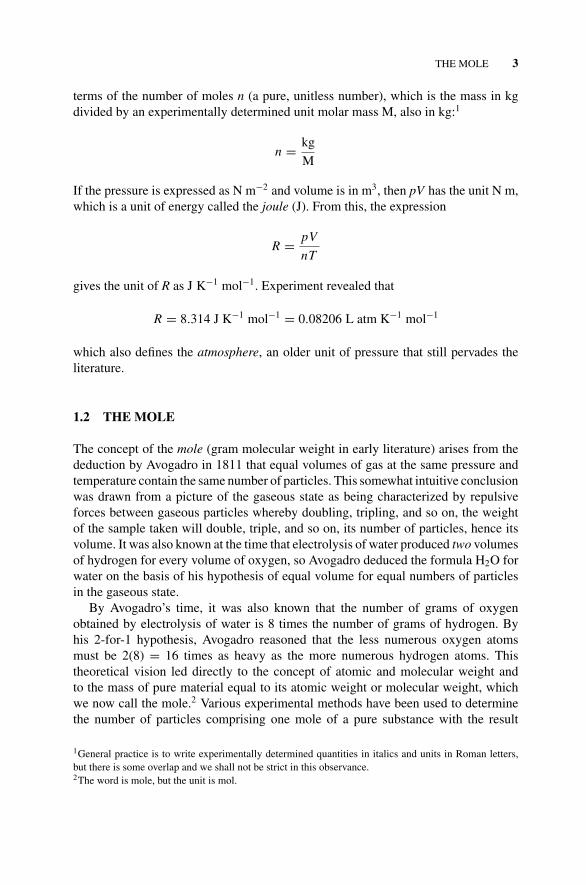
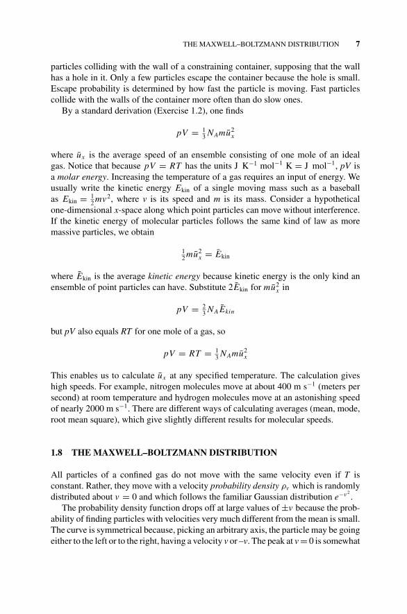
All particles of a confined gas do not move with the same velocity even if T isconstant. Rather, they move with a velocity probability density ρv which is randomlydistributed about v = 0 and which follows the familiar Gaussian distribution e−v2
.The probability density function drops off at large values of ±v because the prob-
ability of finding particles with velocities very much different from the mean is small.The curve is symmetrical because, picking an arbitrary axis, the particle may be goingeither to the left or to the right, having a velocity v or –v. The peak at v = 0 is somewhat
P1: OTA/XYZ P2: ABCc01 JWBS043-Rogers September 13, 2010 11:20 Printer Name: Yet to Come
8 IDEAL GAS LAWS
1
0
ev
2−
33− v
FIGURE 1.1 The probability density for velocities of ideal gas particles at T �= 0.
misleading because it may suggest that the most probable velocity is zero. Not so. Theparticles are not standing still at any temperature above absolute zero. The peak atv = 0 arises because we don’t know which direction any particle is going, left orright. In our ignorance, assuming a random distribution, the best bet is to guess zero.We will always be wrong, but the sum of squares of our error over many trials willbe minimized. This is an example of the principle of least squares.
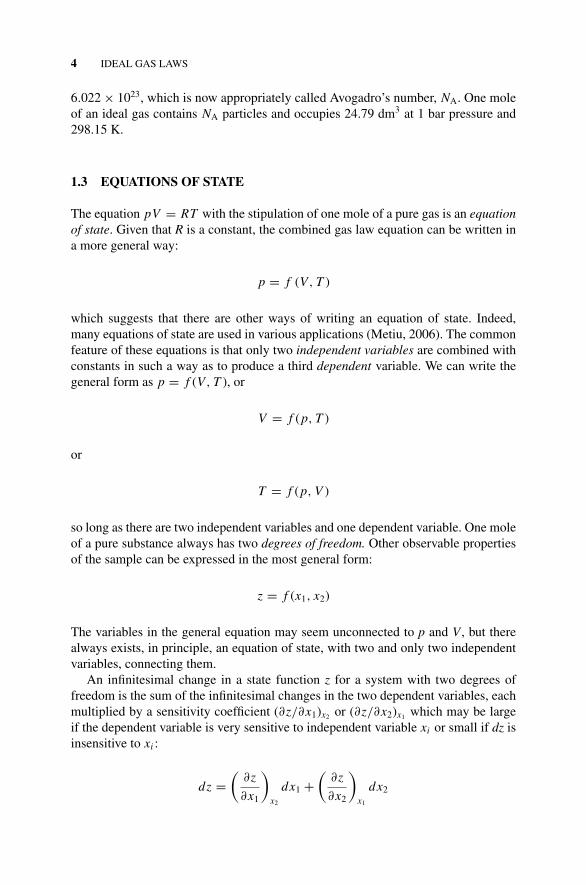
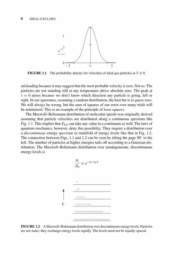
The Maxwell–Boltzmann distribution of molecular speeds was originally derivedassuming that particle velocities are distributed along a continuous spectrum likeFig. 1.1. This implies that Ekin can take any value in a continuum as well. The laws ofquantum mechanics, however, deny this possibility. They require a distribution overa discontinuous energy spectrum or manifold of energy levels like that in Fig. 1.2.The connection between Figs. 1.1 and 1.2 can be seen by tilting the page 90◦ to theleft. The number of particles at higher energies tails off according to a Gaussian dis-tribution. The Maxwell–Boltzmann distribution over nondegenerate, discontinuousenergy levels is
Ni
N0= e−Ei /kB T
. . . . . . . . . . . . . . . . . . . .
. . . . . . . . . . . . . . . .
. . . . . . . . .. . . . .
. .
.
E
FIGURE 1.2 A Maxwell–Boltzmann distribution over discontinuous energy levels. Particlesare not static; they exchange energy levels rapidly. The levels need not be equally spaced.
P1: OTA/XYZ P2: ABCc01 JWBS043-Rogers September 13, 2010 11:20 Printer Name: Yet to Come
A DIGRESSION ON “SPACE” 9
where Ni is the number of particles at the level having energy Ei . In this expression,N0 is the number at the lowest energy, usually designated zero E0 = 0 in the absenceof a reason to do otherwise.4 Energy, being a scalar, is proportional to the squareof the speed of an ensemble of molecules. The population of the energy levels inFig. 1.2 drops off rapidly at higher energies.
The term degeneracy is used when two or more levels exist at the same en-ergy, which sometimes happens under the laws of quantum mechanics. Now thenumber of particles at level Ei is multiplied by the number of levels gi having thatenergy
Ni
N0= gi e
−Ei /kB T
The degeneracy is always an integer and it is usually small. Also, from Ekin = 32 RT
for one mole, we can find the expectation value 〈εkin〉 of the kinetic energy perrepresentative or average particle
〈εkin〉 = 3
2
R
NAT
This leads to the important constant
R
NA= kB = 8.3145
6.022 × 1023= 1.381 × 10⁻²³J K−1
and
〈εkin〉 = 32 kB T
where kB , the universal gas constant per particle, is called the Boltzmann constant. Itshould be evident that kB T must have the units of energy because Ni/N0 is a unitless(pure) number, ln (Ni/N0) = −Ei/kB T , which is also unitless, hence the units ofkB T must be the same as Ei . We are taking advantage of the fact that if y = ex , thenln y = x .
1.9 A DIGRESSION ON “SPACE”
The terms density and probability density were used in Section 1.8. These are differentbut analogous uses of the word density. In the first case, density was used in the usualsense of weight or mass per unit volume, m/V . In the second case, the probabilitydensity is defined as the probability in a specified space. Any variable measured
4Like all energies, this zero point is arbitrary.
P1: OTA/XYZ P2: ABCc01 JWBS043-Rogers September 13, 2010 11:20 Printer Name: Yet to Come
10 IDEAL GAS LAWS
x
y
z
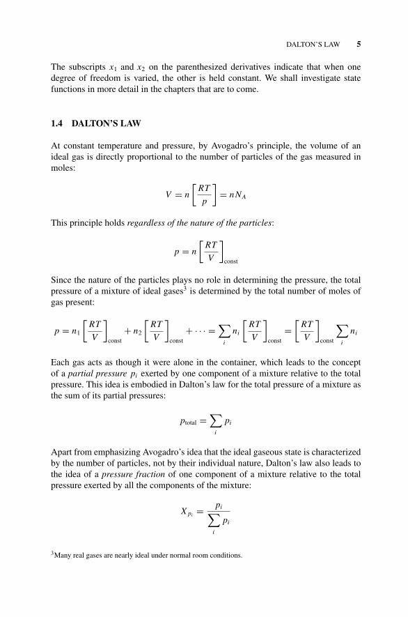
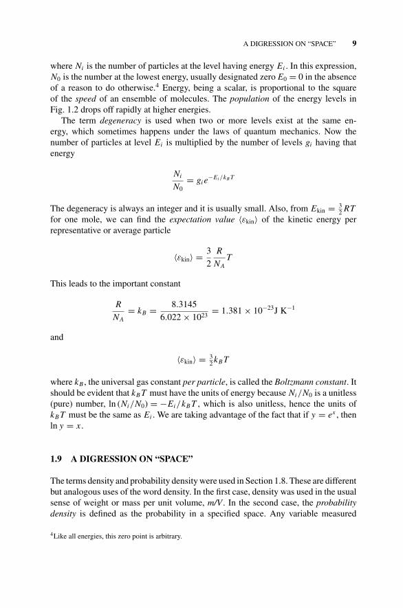
FIGURE 1.3 The Gaussian Probability Density Distribution in 3-Space. The distributioncurve is in the fourth dimension of the space. The probability maximum is at the center of thesphere.
along an axis defines a space. For example, plotting x along a horizontal axis definesa one-dimensional x-space. Space in the x, y, and z dimensions is the familiar 3-spaceoften called a Cartesian space in honor of the seventeenth-century mathematician andphilosopher Rene Descartes. We usually plot functions along mutually perpendicularor orthogonal axes for mathematical convenience. If velocity is plotted along a vaxis, we have a one-dimensional velocity space. If probability density ρ is plottedalong one axis, and velocity is plotted along another axis, the result is a probabilitydensity–velocity space of two dimensions. If ρ(v) is plotted in vx ,vy space, the resultis a function in 3-space; or if it is thought of as a function of all three Cartesiancoordinates, the resulting function is in 4-space. That is, ρ(v) in 1-, 2-, or 3-spacegives a function in 2-, 3-, or 4-space, one dimension more. There should be nothingterrifying about many-dimensional space or hyperspace; it is merely an algebraicgeneralization of the more commonplace use of the term.
The four-dimensional surface of the Gaussian distribution in Cartesian 3-spacecannot be precisely drawn but it can be imagined as a figure with spherical symmetry,having a maximum at the center of the sphere. Imagine that the sphere in Fig. 1.3can be rotated any amount in any angular direction, leaving the distribution curveunchanged.
1.10 THE SUM-OVER-STATES OR PARTITION FUNCTION
Adding up all the particles in all the states of a system gives the total number ofparticles in the system:
∑Ni = N
P1: OTA/XYZ P2: ABCc01 JWBS043-Rogers September 13, 2010 11:20 Printer Name: Yet to Come
THE SUM-OVER-STATES OR PARTITION FUNCTION 11
or
∑Ni =
∑N0gi e
−εi /kB T = N
Since N0 is a number appearing in each term of the sum, it can be factored out:
N0
∑gi e
−εi /kB T = N
Dividing Ni = N0gi e−εi /kB T by N0∑
gi e−εi /kB T = N , gives
Ni
N= N0gi e−εi /kB T
N0
∑gi e
−εi /kB T= gi e−εi /kB T
Q
where we have given the symbol Q to the summation∑
gi e−εi /kB T . This importantsummation appears frequently and is given the name sum-over-states or partitionfunction. Rewriting the ratio Ni/N , we have
Ni Q = Ngi e−εi /kB T︸ ︷︷ ︸
fixed at T = const
We see that, for a given number of molecules N at temperature T , the right handside of the equation is fixed for any specific energy state, that is, Ni Q = const.The sum-over-states is then a scaling factor, determining the relative population of astate, Ni = const/Q. If Q is large, the state is sparsely populated. If Q is small, it isdensely populated. Another way of looking at Q is that it is an indicator of the numberof quantum states available to a system. For many available states (large Q) a givenstate is less densely populated than it would be if only a few states were available(small Q).
The occupation number of a quantum state relative to the total number of particlesNi/N is, strictly speaking, a probability; however, given the immense number ofparticles in a mole of gas, we may treat it as a certainty. The summation of allpossible fractions Ni/N must be 1:
∑i
Ni
N=
∑i
Ni
N= N
N= 1
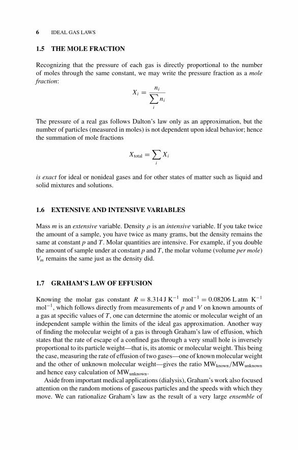
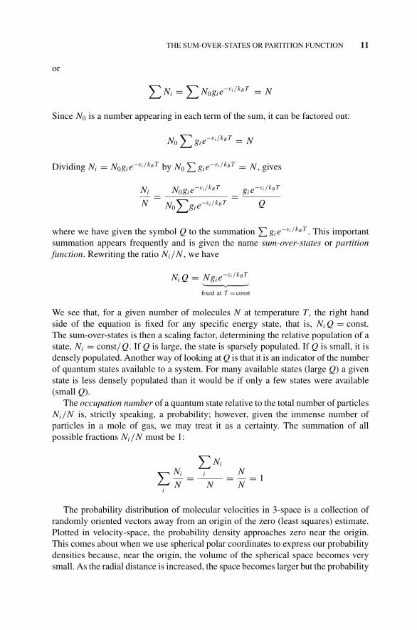
The probability distribution of molecular velocities in 3-space is a collection ofrandomly oriented vectors away from an origin of the zero (least squares) estimate.Plotted in velocity-space, the probability density approaches zero near the origin.This comes about when we use spherical polar coordinates to express our probabilitydensities because, near the origin, the volume of the spherical space becomes verysmall. As the radial distance is increased, the space becomes larger but the probability
P1: OTA/XYZ P2: ABCc01 JWBS043-Rogers September 13, 2010 11:20 Printer Name: Yet to Come
12 IDEAL GAS LAWS
P(v)
v
FIGURE 1.4 The probability density of molecular velocities in a spherical velocity space.
density drops off as a Gaussian function. In between these two approaches to zero,the probability density must go through a maximum as shown in Fig. 1.4.
PROBLEMS AND EXERCISES
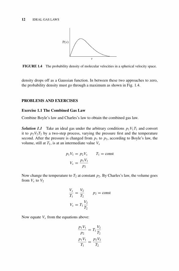
Exercise 1.1 The Combined Gas Law
Combine Boyle’s law and Charles’s law to obtain the combined gas law.
Solution 1.1 Take an ideal gas under the arbitrary conditions p1V1T1 and convertit to p2V2T2 by a two-step process, varying the pressure first and the temperaturesecond. After the pressure is changed from p1 to p2, according to Boyle’s law, thevolume, still at T1, is at an intermediate value Vx
p1V1 = p2Vx T1 = const
Vx = p1V1
p2
Now change the temperature to T2 at constant p2. By Charles’s law, the volume goesfrom Vx to V2
Vx
T1= V2
T2p2 = const
Vx = T1V2
T2
Now equate Vx from the equations above:
p1V1
p2= T1
V2
T2
p1V1
T1= p2V2
T2
P1: OTA/XYZ P2: ABCc01 JWBS043-Rogers September 13, 2010 11:20 Printer Name: Yet to Come
PROBLEMS AND EXERCISES 13
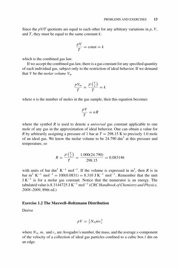
Since the pV/T quotients are equal to each other for any arbitrary variations in p, V ,and T , they must be equal to the same constant k:
pV
T= const = k
which is the combined gas law.If we accept the combined gas law, there is a gas constant for any specified quantity
of each individual gas, subject only to the restriction of ideal behavior. If we demandthat V be the molar volume Vm
pVm
T= p
(Vn
)T
= k
where n is the number of moles in the gas sample, then this equation becomes
pV
T= n R
where the symbol R is used to denote a universal gas constant applicable to onemole of any gas in the approximation of ideal behavior. One can obtain a value forR by arbitrarily assigning a pressure of 1 bar at T = 298.15 K to precisely 1.0 moleof an ideal gas. We know the molar volume to be 24.790 dm3 at this pressure andtemperature, so
R = p(
Vn
)T
= 1.000(24.790)
298.15= 0.083146
with units of bar dm3 K−1 mol−1. If the volume is expressed in m3, then R is inbar m3 K−1 mol−1 = 100(0.0831) = 8.310 J K−1 mol−1. Remember that the unitJ K−1 is for a molar gas constant. Notice that the numerator is an energy. Thetabulated value is 8.3144725 J K−1 mol−1 (CRC Handbook of Chemistry and Physics,2008–2009, 89th ed.)
Exercise 1.2 The Maxwell–Boltzmann Distribution
Derive
pV = 13 NAmv2
x
where NA, m, and vx are Avogadro’s number, the mass, and the average x-componentof the velocity of a collection of ideal gas particles confined to a cubic box l dm onan edge.
P1: OTA/XYZ P2: ABCc01 JWBS043-Rogers September 13, 2010 11:20 Printer Name: Yet to Come
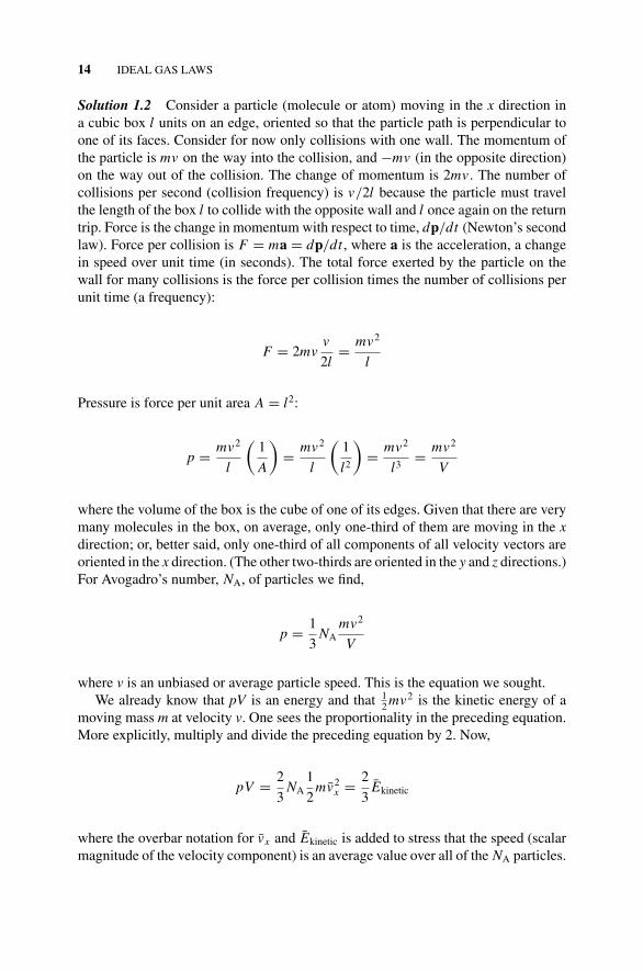
14 IDEAL GAS LAWS
Solution 1.2 Consider a particle (molecule or atom) moving in the x direction ina cubic box l units on an edge, oriented so that the particle path is perpendicular toone of its faces. Consider for now only collisions with one wall. The momentum ofthe particle is mv on the way into the collision, and −mv (in the opposite direction)on the way out of the collision. The change of momentum is 2mv . The number ofcollisions per second (collision frequency) is v/2l because the particle must travelthe length of the box l to collide with the opposite wall and l once again on the returntrip. Force is the change in momentum with respect to time, dp/dt (Newton’s secondlaw). Force per collision is F = ma = dp/dt , where a is the acceleration, a changein speed over unit time (in seconds). The total force exerted by the particle on thewall for many collisions is the force per collision times the number of collisions perunit time (a frequency):
F = 2mvv
2l= mv2
l
Pressure is force per unit area A = l2:
p = mv2
l
(1
A
)= mv2
l
(1
l2
)= mv2
l3= mv2
V
where the volume of the box is the cube of one of its edges. Given that there are verymany molecules in the box, on average, only one-third of them are moving in the xdirection; or, better said, only one-third of all components of all velocity vectors areoriented in the x direction. (The other two-thirds are oriented in the y and z directions.)For Avogadro’s number, NA, of particles we find,
p = 1
3NA
mv2
V
where v is an unbiased or average particle speed. This is the equation we sought.We already know that pV is an energy and that 1
2 mv2 is the kinetic energy of amoving mass m at velocity v. One sees the proportionality in the preceding equation.More explicitly, multiply and divide the preceding equation by 2. Now,
pV = 2
3NA
1
2mv2
x = 2
3Ekinetic
where the overbar notation for vx and Ekinetic is added to stress that the speed (scalarmagnitude of the velocity component) is an average value over all of the NA particles.
P1: OTA/XYZ P2: ABCc01 JWBS043-Rogers September 13, 2010 11:20 Printer Name: Yet to Come
PROBLEMS AND EXERCISES 15
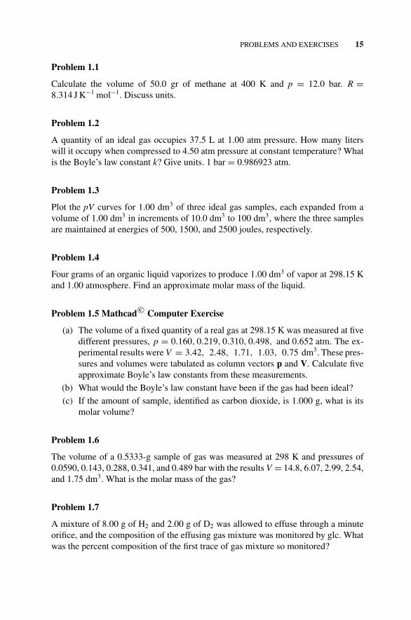
Problem 1.1
Calculate the volume of 50.0 gr of methane at 400 K and p = 12.0 bar. R =8.314 J K−1 mol−1. Discuss units.
Problem 1.2
A quantity of an ideal gas occupies 37.5 L at 1.00 atm pressure. How many literswill it occupy when compressed to 4.50 atm pressure at constant temperature? Whatis the Boyle’s law constant k? Give units. 1 bar = 0.986923 atm.
Problem 1.3
Plot the pV curves for 1.00 dm3 of three ideal gas samples, each expanded from avolume of 1.00 dm3 in increments of 10.0 dm3 to 100 dm3, where the three samplesare maintained at energies of 500, 1500, and 2500 joules, respectively.
Problem 1.4
Four grams of an organic liquid vaporizes to produce 1.00 dm3 of vapor at 298.15 Kand 1.00 atmosphere. Find an approximate molar mass of the liquid.
Problem 1.5 Mathcad C© Computer Exercise
(a) The volume of a fixed quantity of a real gas at 298.15 K was measured at fivedifferent pressures, p = 0.160, 0.219, 0.310, 0.498, and 0.652 atm. The ex-perimental results were V = 3.42, 2.48, 1.71, 1.03, 0.75 dm3. These pres-sures and volumes were tabulated as column vectors p and V. Calculate fiveapproximate Boyle’s law constants from these measurements.
(b) What would the Boyle’s law constant have been if the gas had been ideal?
(c) If the amount of sample, identified as carbon dioxide, is 1.000 g, what is itsmolar volume?
Problem 1.6
The volume of a 0.5333-g sample of gas was measured at 298 K and pressures of0.0590, 0.143, 0.288, 0.341, and 0.489 bar with the results V = 14.8, 6.07, 2.99, 2.54,and 1.75 dm3. What is the molar mass of the gas?
Problem 1.7
A mixture of 8.00 g of H2 and 2.00 g of D2 was allowed to effuse through a minuteorifice, and the composition of the effusing gas mixture was monitored by glc. Whatwas the percent composition of the first trace of gas mixture so monitored?

P1: OTA/XYZ P2: ABCc01 JWBS043-Rogers September 13, 2010 11:20 Printer Name: Yet to Come
16 IDEAL GAS LAWS
Problem 1.8
We have two expressions for the molar volume of an ideal gas: (1) Vm = 22.414 Lat 0◦C and 1 atm and (2) Vm = 24.790 dm3 at 25◦C and 1 bar. (The atm and barare taken to have an indefinite number of significant digits.) Use this information toobtain absolute zero (T = 0 K) on the Centigrade scale.
Problem 1.9
If a gas occupies 47.6 dm3 at NSTP = 298.15 K, what is its volume at 1.00 bar and500 K? The acronym for new standard temperature and pressure NSTP replaces theold STP for standard temperature and pressure.
Problem 1.10
(a) Suppose that 18.44 g of N2 occupies a container at new standard temperatureand pressure NSTP and 24.35 g of a sample of a different gas is introduced intothe container, keeping the temperature constant. If the pressure after additionis 3.20 bar, what is the average molar mass Mav of the mixture?
(b) What is the molar mass of the introduced gas?
Problem 1.11
A pure gas takes twice as long as helium to effuse through a porous membrane. Whatis its molar mass?
Problem 1.12
Compute the root mean square speed of H2 molecules at 1000 K.
Problem 1.13
What is the translational energy of 1 mol of an ideal gas at T = 298.15 K?
Computer Exercise 1.14
Using a standard plotting package, plot a graph of pV = k where k = 1, taking p asthe vertical axis and V as the horizontal axis. Play with your plotting package so as toproduce many different plots, thereby learning the idiosyncrasies of your particularpackage.
Problem 1.15
What is the expectation value of the molecular speed among an ensemble of nitrogenmolecules at 298 K?

P1: OTA/XYZ P2: ABCc01 JWBS043-Rogers September 13, 2010 11:20 Printer Name: Yet to Come
PROBLEMS AND EXERCISES 17
Problem 1.16
(a) Calculate the expectation value of the speed of hydrogen molecules amongan ensemble at 298 K. Give units.
(b) At the same temperature, 〈v〉 = 515 m s−1 for nitrogen molecules. What is theratio 〈vH2〉/〈vN2〉? Explain this ratio. Give units.
Problem 1.17
A sample of 2.50 mol of a gas was confined to a certain volume at 1.00 atm pressureand 298 K. Assuming ideal behavior, what volume did it occupy?
Problem 1.18
If the molar volume is 24.79 dm3 at 298.15 K and 1 bar pressure, what is the universalgas constant. Give units.
P1: OTA/XYZ P2: ABCc02 JWBS043-Rogers September 13, 2010 11:23 Printer Name: Yet to Come
2REAL GASES:EMPIRICAL EQUATIONS
The ideal gas laws are based on two assumptions, neither of which is true. First,atoms or molecules comprising the ideal gas are assumed to have no volume. Theyare treated as mathematical point masses for convenience. Second, they are assumedto have no interactions with each other. Attractive and repulsive forces are ignoredby setting them to zero.
2.1 THE VAN DER WAALS EQUATION
The Dutch physicist van der Waals remedied both of these failures. He treated the firstof them by simply subtracting an empirical parameter taken to represent the volumeof the particles, called the excluded volume b, from the total volume V of the gas toleave an effective volume of (V – b). There is less space for each molecule to move inbecause of the space taken up by its neighbors.
Attractive and repulsive forces often operate through an inverse square law. Forexample, gravitational force on masses m1 and m2 at a separation of r is
F = Gm1m2
r2
where G is the gravitational constant. The constants G, m1, and m2 can be groupedas a single constant k in the numerator to give an attractive or repulsive force F thatvaries as F = k/r2. Van der Waals reasoned that the distance between gas particles
Concise Physical Chemistry, by Donald W. RogersCopyright C© 2011 John Wiley & Sons, Inc.
18

P1: OTA/XYZ P2: ABCc02 JWBS043-Rogers September 13, 2010 11:23 Printer Name: Yet to Come
THE VIRIAL EQUATION: A PARAMETRIC CURVE FIT 19
increases directly with the volume occupied by the gas; thus, for the attractive forcebetween particles, he wrote
F = a
V 2
The conversion factor from distance to volume is not needed because it is included inthe parameter a, which is determined experimentally. Pressure is force per unit areaon the walls of a container, so van der Waals added the force term to the pressure andrewrote the ideal gas equation for one mole of a real gas as the corrected pressuretimes the volume remaining after subtracting the volume of the particles:
(p + a
V 2
)(V − b) = RT
The van der Waals equation is a semiempirical equation because the ideal gas law onwhich it is based can be derived from pure theory (see below), but a and b are empiricalparameters found by trial and error. One can start with a pair of plausible estimatesfor a and b, vary them, compare the results with measured p, V, T behavior, and selectthe values of a and b that give the best agreement with experimental measurements.Computer routines are available that make many thousands of estimates and give thebest curve fit in a matter of seconds.
A knowledge of b permits one to calculate order-of-magnitude radii of molecules.For example, the van der Waals radius of methane is 190 pm (picometers, 10−9 m) ascompared to the spectroscopic value (obtained many years later) of 109 pm for theC–H bond length of methane. Numerous similar calculations give comparable results.This rough agreement supports van der Waals’s qualitative picture of the excludedvolume of real gases.
2.2 THE VIRIAL EQUATION: A PARAMETRIC CURVE FIT
The virial equation is an example of a more general and frequently more accuratecurve fitting routine than the van der Waals equation, but it that gives less insight intopossible causes of nonideal behavior than the van der Waals equation does. Any dataset can be graphed and fit by an analytical equation (an equation that can be writtenout in terms of a limited number of variables and some accompanying parameters).A parameter is a number entering into an equation that takes on a fixed value for onesystem but may change to some other fixed value for another system. For example,what is usually called the Boyle’s law “constant” pV = k is, in fact, a parameterbecause it is valid only for a specified, fixed temperature. Change the temperatureand the parameter takes on a different value, but it acts like a constant as long as youmaintain the temperature fixed. The gas law constant R is a true constant; for onemole of an ideal gas it is always the same.
Of any two equations, one will be a better fit to a given data set than the other.Of three equations, one will be a better fit than either of the other two, and so on.
P1: OTA/XYZ P2: ABCc02 JWBS043-Rogers September 13, 2010 11:23 Printer Name: Yet to Come
20 REAL GASES: EMPIRICAL EQUATIONS
Computer speed makes it possible to try very many equations and select the best one,but there is a point of diminishing returns. An equation may have so many parametersthat no one will ever use it or it may follow random fluctuations in the data set thattell us nothing about the physics of the actual system. If you are not prudent in youruse of curve-fitting programs, you may be calculating the characteristics of a unicornto many significant figures. These caveats apply to any curve-fitting problem, not justthose of real gases.
A very nice balance that avoids daunting complexity but achieves good accuracyis the series equation
y = a + bx + cx2 + dx3 + · · ·
which has an infinite number of terms but which is cut off or truncated at somereasonable number of terms, usually 3 or 4. As applied to real gases, this series is thevirial equation of state:
pVm = RT + B2 [T ]
(RT
Vm
)+ B3 [T ]
(RT
Vm
)2
+ B4 [T ]
(RT
Vm
)3
+ · · ·
The parameters B2 [T ], B3 [T ], and B4 [T ] are called the second, third, fourth, . . .
virial coefficients and the notation Vm = V/n is used to remind us that the volumetaken is a molar quantity. The notation B2 [T ], B3 [T ], B4 [T ], . . . is used to indicatetemperature dependence of the virial coefficients. The square brackets do not indicatemultiplication. By a simple algebraic manipulation, it is possible to express the virialcoefficients in terms of the van der Waals constants and find B2 [T ] = b − a/RT . Byanother simple manipulation, one obtains the compressibility factor.
2.3 THE COMPRESSIBILITY FACTOR
The difference between ideal and real gaseous behavior can be made clearer if wedefine a compressibility factor Z, a way of indicating the degree of nonideality ofa gas
Z = pVm
RT= pVm
(pVm)ideal
If Z is less than one, nonideality is largely due to attractive forces between molecules.If Z is greater than one, the nonideal behavior can be ascribed to the volume takenup by individual molecules treated as hard spheres or to repulsive forces, or both.An ideal gas would show a compressibility factor of 1.00 at all pressures. At hightemperatures, the total volume is large for any selected pressure. Molecular crowdingbecomes less significant, and attractive or repulsive forces are weaker because theyact over longer distances. The gas approaches ideal behavior and Z approaches theconstant value of 1.00 as p approaches zero.
P1: OTA/XYZ P2: ABCc02 JWBS043-Rogers September 13, 2010 11:23 Printer Name: Yet to Come
THE COMPRESSIBILITY FACTOR 21
Pressure
2520151050
Com
pres
sibi
lity
Fact
or, Z
0.9840
0.9845
0.9850
0.9855
0.9860
0.9865
0.9870
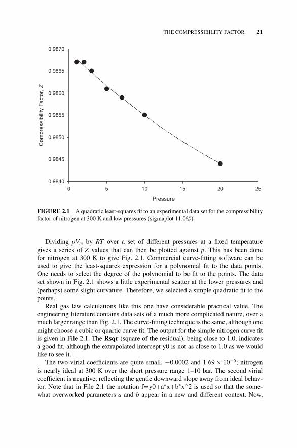
FIGURE 2.1 A quadratic least-squares fit to an experimental data set for the compressibilityfactor of nitrogen at 300 K and low pressures (sigmaplot 11.0 C©).
Dividing pVm by RT over a set of different pressures at a fixed temperaturegives a series of Z values that can then be plotted against p. This has been donefor nitrogen at 300 K to give Fig. 2.1. Commercial curve-fitting software can beused to give the least-squares expression for a polynomial fit to the data points.One needs to select the degree of the polynomial to be fit to the points. The dataset shown in Fig. 2.1 shows a little experimental scatter at the lower pressures and(perhaps) some slight curvature. Therefore, we selected a simple quadratic fit to thepoints.
Real gas law calculations like this one have considerable practical value. Theengineering literature contains data sets of a much more complicated nature, over amuch larger range than Fig. 2.1. The curve-fitting technique is the same, although onemight choose a cubic or quartic curve fit. The output for the simple nitrogen curve fitis given in File 2.1. The Rsqr (square of the residual), being close to 1.0, indicatesa good fit, although the extrapolated intercept y0 is not as close to 1.0 as we wouldlike to see it.
The two virial coefficients are quite small, −0.0002 and 1.69 × 10⁻⁶; nitrogenis nearly ideal at 300 K over the short pressure range 1–10 bar. The second virialcoefficient is negative, reflecting the gentle downward slope away from ideal behav-ior. Note that in File 2.1 the notation f=y0+a∗x+b∗x∧2 is used so that the some-what overworked parameters a and b appear in a new and different context. Now,
P1: OTA/XYZ P2: ABCc02 JWBS043-Rogers September 13, 2010 11:23 Printer Name: Yet to Come
22 REAL GASES: EMPIRICAL EQUATIONS
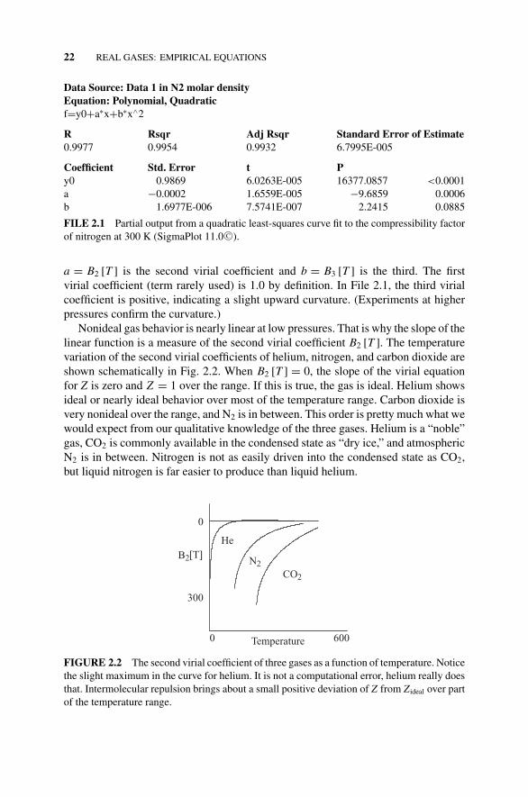
Data Source: Data 1 in N2 molar densityEquation: Polynomial, Quadraticf=y0+a∗x+b∗x∧2
R Rsqr Adj Rsqr Standard Error of Estimate0.9977 0.9954 0.9932 6.7995E-005
Coefficient Std. Error t Py0 0.9869 6.0263E-005 16377.0857 <0.0001a −0.0002 1.6559E-005 −9.6859 0.0006b 1.6977E-006 7.5741E-007 2.2415 0.0885
FILE 2.1 Partial output from a quadratic least-squares curve fit to the compressibility factorof nitrogen at 300 K (SigmaPlot 11.0 C©).
a = B2 [T ] is the second virial coefficient and b = B3 [T ] is the third. The firstvirial coefficient (term rarely used) is 1.0 by definition. In File 2.1, the third virialcoefficient is positive, indicating a slight upward curvature. (Experiments at higherpressures confirm the curvature.)
Nonideal gas behavior is nearly linear at low pressures. That is why the slope of thelinear function is a measure of the second virial coefficient B2 [T ]. The temperaturevariation of the second virial coefficients of helium, nitrogen, and carbon dioxide areshown schematically in Fig. 2.2. When B2 [T ] = 0, the slope of the virial equationfor Z is zero and Z = 1 over the range. If this is true, the gas is ideal. Helium showsideal or nearly ideal behavior over most of the temperature range. Carbon dioxide isvery nonideal over the range, and N2 is in between. This order is pretty much what wewould expect from our qualitative knowledge of the three gases. Helium is a “noble”gas, CO2 is commonly available in the condensed state as “dry ice,” and atmosphericN2 is in between. Nitrogen is not as easily driven into the condensed state as CO2,but liquid nitrogen is far easier to produce than liquid helium.
0
300
He
N2CO2
B2
Temperature
[T]
0060
FIGURE 2.2 The second virial coefficient of three gases as a function of temperature. Noticethe slight maximum in the curve for helium. It is not a computational error, helium really doesthat. Intermolecular repulsion brings about a small positive deviation of Z from Zideal over partof the temperature range.
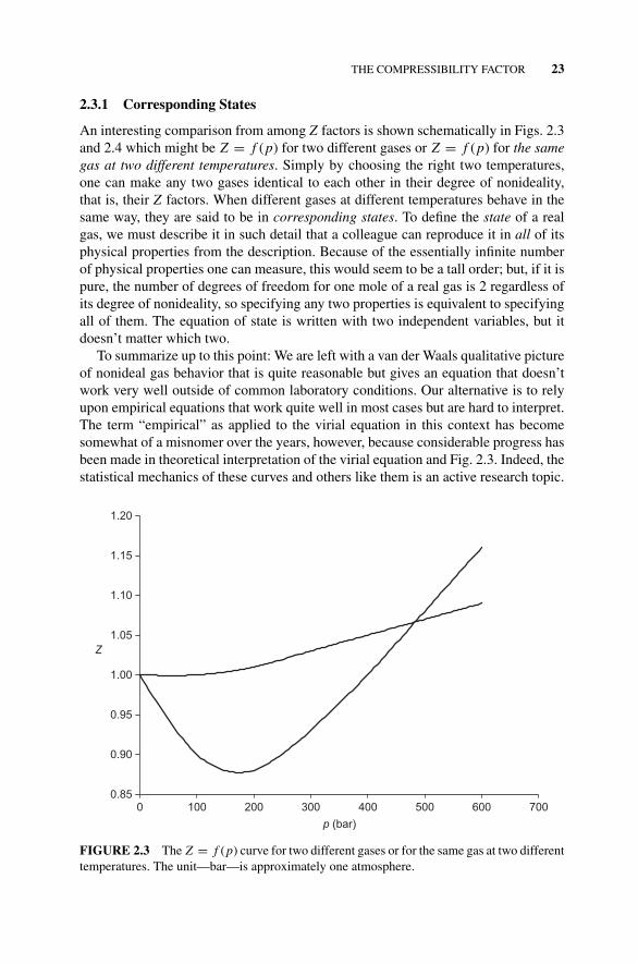
P1: OTA/XYZ P2: ABCc02 JWBS043-Rogers September 13, 2010 11:23 Printer Name: Yet to Come
THE COMPRESSIBILITY FACTOR 23
2.3.1 Corresponding States
An interesting comparison from among Z factors is shown schematically in Figs. 2.3and 2.4 which might be Z = f (p) for two different gases or Z = f (p) for the samegas at two different temperatures. Simply by choosing the right two temperatures,one can make any two gases identical to each other in their degree of nonideality,that is, their Z factors. When different gases at different temperatures behave in thesame way, they are said to be in corresponding states. To define the state of a realgas, we must describe it in such detail that a colleague can reproduce it in all of itsphysical properties from the description. Because of the essentially infinite numberof physical properties one can measure, this would seem to be a tall order; but, if it ispure, the number of degrees of freedom for one mole of a real gas is 2 regardless ofits degree of nonideality, so specifying any two properties is equivalent to specifyingall of them. The equation of state is written with two independent variables, but itdoesn’t matter which two.
To summarize up to this point: We are left with a van der Waals qualitative pictureof nonideal gas behavior that is quite reasonable but gives an equation that doesn’twork very well outside of common laboratory conditions. Our alternative is to relyupon empirical equations that work quite well in most cases but are hard to interpret.The term “empirical” as applied to the virial equation in this context has becomesomewhat of a misnomer over the years, however, because considerable progress hasbeen made in theoretical interpretation of the virial equation and Fig. 2.3. Indeed, thestatistical mechanics of these curves and others like them is an active research topic.
p (bar)
7006005004003002001000
Z
0.85
0.90
0.95
1.00
1.05
1.10
1.15
1.20
FIGURE 2.3 The Z = f (p) curve for two different gases or for the same gas at two differenttemperatures. The unit—bar—is approximately one atmosphere.
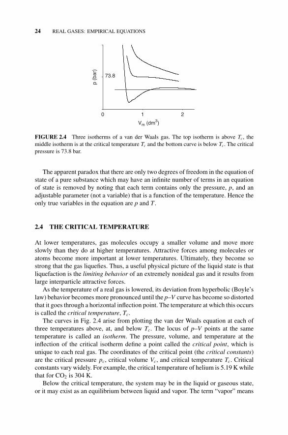
P1: OTA/XYZ P2: ABCc02 JWBS043-Rogers September 13, 2010 11:23 Printer Name: Yet to Come
24 REAL GASES: EMPIRICAL EQUATIONS
Vm (dm3)
210
p (b
ar)
73.8
FIGURE 2.4 Three isotherms of a van der Waals gas. The top isotherm is above Tc, themiddle isotherm is at the critical temperature Tc and the bottom curve is below Tc. The criticalpressure is 73.8 bar.
The apparent paradox that there are only two degrees of freedom in the equation ofstate of a pure substance which may have an infinite number of terms in an equationof state is removed by noting that each term contains only the pressure, p, and anadjustable parameter (not a variable) that is a function of the temperature. Hence theonly true variables in the equation are p and T .
2.4 THE CRITICAL TEMPERATURE
At lower temperatures, gas molecules occupy a smaller volume and move moreslowly than they do at higher temperatures. Attractive forces among molecules oratoms become more important at lower temperatures. Ultimately, they become sostrong that the gas liquefies. Thus, a useful physical picture of the liquid state is thatliquefaction is the limiting behavior of an extremely nonideal gas and it results fromlarge interparticle attractive forces.
As the temperature of a real gas is lowered, its deviation from hyperbolic (Boyle’slaw) behavior becomes more pronounced until the p–V curve has become so distortedthat it goes through a horizontal inflection point. The temperature at which this occursis called the critical temperature, Tc.
The curves in Fig. 2.4 arise from plotting the van der Waals equation at each ofthree temperatures above, at, and below Tc. The locus of p–V points at the sametemperature is called an isotherm. The pressure, volume, and temperature at theinflection of the critical isotherm define a point called the critical point, which isunique to each real gas. The coordinates of the critical point (the critical constants)are the critical pressure pc, critical volume Vc, and critical temperature Tc. Criticalconstants vary widely. For example, the critical temperature of helium is 5.19 K whilethat for CO2 is 304 K.
Below the critical temperature, the system may be in the liquid or gaseous state,or it may exist as an equilibrium between liquid and vapor. The term “vapor” means
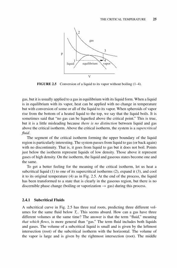
P1: OTA/XYZ P2: ABCc02 JWBS043-Rogers September 13, 2010 11:23 Printer Name: Yet to Come
THE CRITICAL TEMPERATURE 25
1
2
3p
V
4
gas
liquid equilibrium vapor
FIGURE 2.5 Conversion of a liquid to its vapor without boiling (1–4).
gas, but it is usually applied to a gas in equilibrium with its liquid form. When a liquidis in equilibrium with its vapor, heat can be applied with no change in temperaturebut with conversion of some or all of the liquid to its vapor. When spheroids of vaporrise from the bottom of a heated liquid to the top, we say that the liquid boils. It issometimes said that “no gas can be liquefied above the critical point.” This is true,but it is a little misleading because there is no distinction between liquid and gasabove the critical isotherm. Above the critical isotherm, the system is a supercriticalfluid.
The segment of the critical isotherm forming the upper boundary of the liquidregion is particularly interesting. The system passes from liquid to gas (or back again)with no discontinuity. That is, it goes from liquid to gas but it does not boil. Pointsjust below the isotherm represent liquids of low density. Those above it representgases of high density. On the isotherm, the liquid and gaseous states become one andthe same.
To get a better feeling for the meaning of the critical isotherm, let us heat asubcritical liquid (1) to one of its supercritical isotherms (2), expand it (3), and coolit to its original temperature (4) as in Fig. 2.5. At the end of the process, the liquidhas been transformed to a state that is clearly in the gaseous region, but there is nodiscernible phase change (boiling or vaporization → gas) during this process.
2.4.1 Subcritical Fluids
A subcritical curve in Fig. 2.5 has three real roots, predicting three different vol-umes for the same fluid below Tc. This seems absurd. How can a gas have threedifferent volumes at the same time? The answer is that the term “fluid,” meaningthat which flows, is more general than “gas.” The term fluid includes both liquidsand gases. The volume of a subcritical liquid is small and is given by the leftmostintersection (root) of the subcritical isotherm with the horizontal. The volume ofthe vapor is large and is given by the rightmost intersection (root). The middle
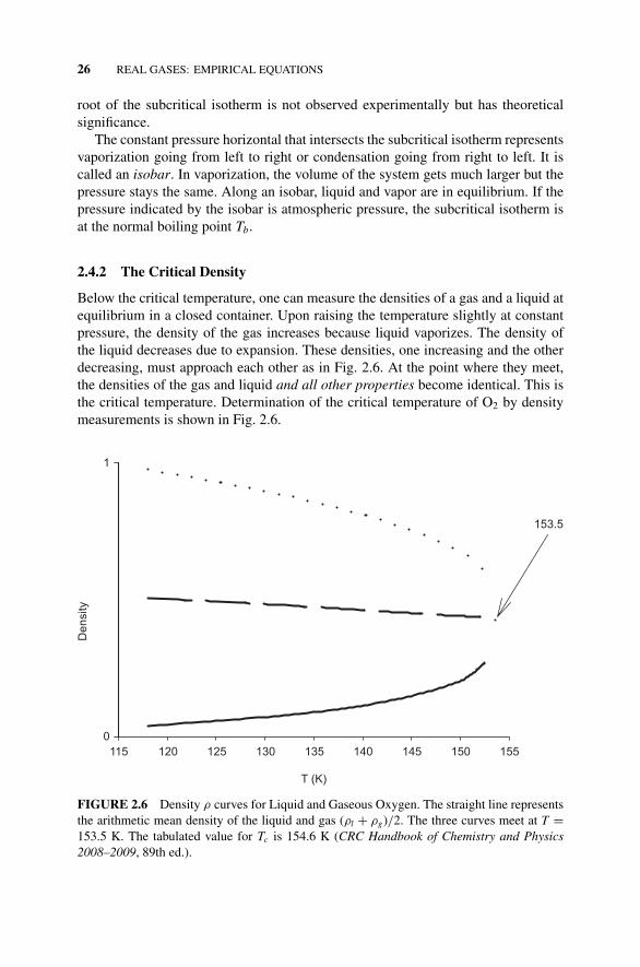
P1: OTA/XYZ P2: ABCc02 JWBS043-Rogers September 13, 2010 11:23 Printer Name: Yet to Come
26 REAL GASES: EMPIRICAL EQUATIONS
root of the subcritical isotherm is not observed experimentally but has theoreticalsignificance.
The constant pressure horizontal that intersects the subcritical isotherm representsvaporization going from left to right or condensation going from right to left. It iscalled an isobar. In vaporization, the volume of the system gets much larger but thepressure stays the same. Along an isobar, liquid and vapor are in equilibrium. If thepressure indicated by the isobar is atmospheric pressure, the subcritical isotherm isat the normal boiling point Tb.
2.4.2 The Critical Density
Below the critical temperature, one can measure the densities of a gas and a liquid atequilibrium in a closed container. Upon raising the temperature slightly at constantpressure, the density of the gas increases because liquid vaporizes. The density ofthe liquid decreases due to expansion. These densities, one increasing and the otherdecreasing, must approach each other as in Fig. 2.6. At the point where they meet,the densities of the gas and liquid and all other properties become identical. This isthe critical temperature. Determination of the critical temperature of O2 by densitymeasurements is shown in Fig. 2.6.
T (K)
155150145140135130125120115
De
nsity
0
1
.
153.5
FIGURE 2.6 Density ρ curves for Liquid and Gaseous Oxygen. The straight line representsthe arithmetic mean density of the liquid and gas (ρl + ρg)/2. The three curves meet at T =153.5 K. The tabulated value for Tc is 154.6 K (CRC Handbook of Chemistry and Physics2008–2009, 89th ed.).

P1: OTA/XYZ P2: ABCc02 JWBS043-Rogers September 13, 2010 11:23 Printer Name: Yet to Come
THE LAW OF CORRESPONDING STATES, ANOTHER VIEW 27
2.5 REDUCED VARIABLES
The degree of nonideality for real gases is determined by how near the temperatureis to the critical temperature. We can express the “nearness” of the temperature ofa gas to its critical temperature as the unitless ratio T/Tc. This ratio is called thereduced temperature
TR = T
Tc
The other reduced variables are defined in the same way. The (unitless) reducedpressure and reduced volume are, for one mole,
pR = p
pcand VR = V
Vc
These new variables are scaling factors by which we take an entire family of isothermssuggested by the three representative isotherms in Fig. 2.4 and move, stretch, orcompress them until their critical isotherms coincide. Having done that, at the sameTR , the pR and, VR behavior of all gases fall approximately on the same familyof curves. The gas data have been manipulated into corresponding states (Section2.3). Knowing the behavior of one gas in terms of its reduced variables pR , VR , andTR , we know the behavior of any real gas, provided only that we know its criticalconstants pc, Vc, and Tc. Needless to say, industrial chemists and chemical engineersare delighted by this, and they have devoted considerable effort to construct standardtables and Z-curves in terms of the reduced variables.
2.6 THE LAW OF CORRESPONDING STATES, ANOTHER VIEW
Replacing the parameters a and b and the constant R in the van der Waals equationfor one mole
p = RT
(V − b)− a
V 2
with
b = Vc
3, a = 3pcV 2
c , and R = 8pcVc
3Tc
we get, with some algebraic manipulation (see Problems and Exercise 2.1),
[pR + 3
V 2R
] (VR − 1
3
)= 8
3TR
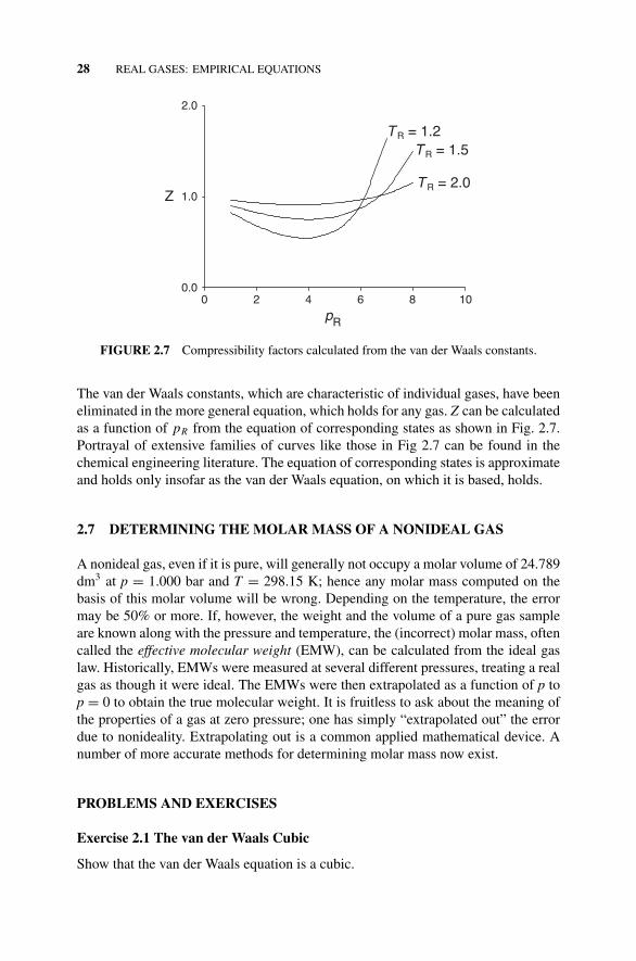
P1: OTA/XYZ P2: ABCc02 JWBS043-Rogers September 13, 2010 11:23 Printer Name: Yet to Come
28 REAL GASES: EMPIRICAL EQUATIONS
pR
1086420
Z 1.0
2.0
0.0
T R = 1.2T R = 1.5
T R = 2.0
FIGURE 2.7 Compressibility factors calculated from the van der Waals constants.
The van der Waals constants, which are characteristic of individual gases, have beeneliminated in the more general equation, which holds for any gas. Z can be calculatedas a function of pR from the equation of corresponding states as shown in Fig. 2.7.Portrayal of extensive families of curves like those in Fig 2.7 can be found in thechemical engineering literature. The equation of corresponding states is approximateand holds only insofar as the van der Waals equation, on which it is based, holds.
2.7 DETERMINING THE MOLAR MASS OF A NONIDEAL GAS
A nonideal gas, even if it is pure, will generally not occupy a molar volume of 24.789dm3 at p = 1.000 bar and T = 298.15 K; hence any molar mass computed on thebasis of this molar volume will be wrong. Depending on the temperature, the errormay be 50% or more. If, however, the weight and the volume of a pure gas sampleare known along with the pressure and temperature, the (incorrect) molar mass, oftencalled the effective molecular weight (EMW), can be calculated from the ideal gaslaw. Historically, EMWs were measured at several different pressures, treating a realgas as though it were ideal. The EMWs were then extrapolated as a function of p top = 0 to obtain the true molecular weight. It is fruitless to ask about the meaning ofthe properties of a gas at zero pressure; one has simply “extrapolated out” the errordue to nonideality. Extrapolating out is a common applied mathematical device. Anumber of more accurate methods for determining molar mass now exist.
PROBLEMS AND EXERCISES
Exercise 2.1 The van der Waals Cubic
Show that the van der Waals equation is a cubic.
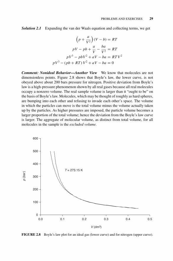
P1: OTA/XYZ P2: ABCc02 JWBS043-Rogers September 13, 2010 11:23 Printer Name: Yet to Come
PROBLEMS AND EXERCISES 29
Solution 2.1 Expanding the van der Waals equation and collecting terms, we get
(p + a
V 2
)(V − b) = RT
pV − pb + a
V− ba
V 2= RT
pV 3 − pbV 2 + aV − ba = RT V 2
pV 3 − (pb + RT ) V 2 + aV − ba = 0
Comment: Nonideal Behavior—Another View We know that molecules are notdimensionless points. Figure 2.8 shows that Boyle’s law, the lower curve, is notobeyed above about 200 bars pressure for nitrogen. Positive deviation from Boyle’slaw is a high-pressure phenomenon shown by all real gases because all real moleculesoccupy a nonzero volume. The real sample volume is larger than it “ought to be” onthe basis of Boyle’s law. Molecules, which may be thought of roughly as hard spheres,are bumping into each other and refusing to invade each other’s space. The volumein which the particles can move is the total volume minus the volume actually takenup by the particles. As higher pressures are imposed, the particle volume becomes alarger proportion of the total volume; hence the deviation from the Boyle’s law curveis larger. The aggregate of molecular volume, as distinct from total volume, for allmolecules in the sample is the excluded volume.
V (dm3)
0.50.40.30.20.10.0
p (b
ar)
0
100
200
300
400
500
600
T = 273.15 K
FIGURE 2.8 Boyle’s law plot for an ideal gas (lower curve) and for nitrogen (upper curve).
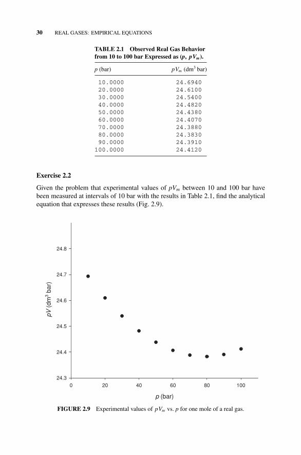
P1: OTA/XYZ P2: ABCc02 JWBS043-Rogers September 13, 2010 11:23 Printer Name: Yet to Come
30 REAL GASES: EMPIRICAL EQUATIONS
TABLE 2.1 Observed Real Gas Behaviorfrom 10 to 100 bar Expressed as (p, pVm).
p (bar) pVm (dm3 bar)
10.0000 24.694020.0000 24.610030.0000 24.540040.0000 24.482050.0000 24.438060.0000 24.407070.0000 24.388080.0000 24.383090.0000 24.3910100.0000 24.4120
Exercise 2.2
Given the problem that experimental values of pVm between 10 and 100 bar havebeen measured at intervals of 10 bar with the results in Table 2.1, find the analyticalequation that expresses these results (Fig. 2.9).
p (bar)
100806040200
pV (
dm3 b
ar)
24.3
24.4
24.5
24.6
24.7
24.8
FIGURE 2.9 Experimental values of pVm vs. p for one mole of a real gas.
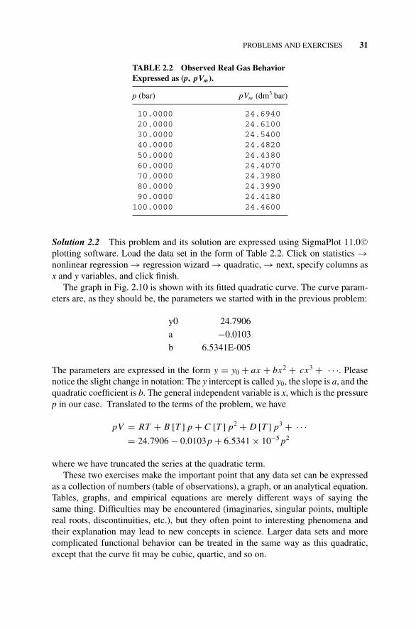
P1: OTA/XYZ P2: ABCc02 JWBS043-Rogers September 13, 2010 11:23 Printer Name: Yet to Come
PROBLEMS AND EXERCISES 31
TABLE 2.2 Observed Real Gas BehaviorExpressed as (p, pVm).
p (bar) pVm (dm3 bar)
10.0000 24.694020.0000 24.610030.0000 24.540040.0000 24.482050.0000 24.438060.0000 24.407070.0000 24.398080.0000 24.399090.0000 24.4180100.0000 24.4600
Solution 2.2 This problem and its solution are expressed using SigmaPlot 11.0 C©plotting software. Load the data set in the form of Table 2.2. Click on statistics →nonlinear regression → regression wizard → quadratic, → next, specify columns asx and y variables, and click finish.
The graph in Fig. 2.10 is shown with its fitted quadratic curve. The curve param-eters are, as they should be, the parameters we started with in the previous problem:
y0 24.7906
a −0.0103
b 6.5341E-005
The parameters are expressed in the form y = y0 + ax + bx2 + cx3 + · · ·. Pleasenotice the slight change in notation: The y intercept is called y0, the slope is a, and thequadratic coefficient is b. The general independent variable is x, which is the pressurep in our case. Translated to the terms of the problem, we have
pV = RT + B [T ] p + C [T ] p2 + D [T ] p3 + · · ·= 24.7906 − 0.0103p + 6.5341 × 10⁻⁵ p2
where we have truncated the series at the quadratic term.These two exercises make the important point that any data set can be expressed
as a collection of numbers (table of observations), a graph, or an analytical equation.Tables, graphs, and empirical equations are merely different ways of saying thesame thing. Difficulties may be encountered (imaginaries, singular points, multiplereal roots, discontinuities, etc.), but they often point to interesting phenomena andtheir explanation may lead to new concepts in science. Larger data sets and morecomplicated functional behavior can be treated in the same way as this quadratic,except that the curve fit may be cubic, quartic, and so on.
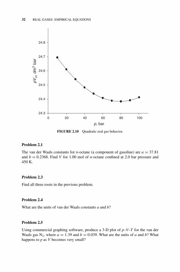
P1: OTA/XYZ P2: ABCc02 JWBS043-Rogers September 13, 2010 11:23 Printer Name: Yet to Come
32 REAL GASES: EMPIRICAL EQUATIONS
p, bar
100806040200
pV ,
dm
ba
rm
3
24.3
24.4
24.5
24.6
24.7
24.8
FIGURE 2.10 Quadratic real gas behavior.
Problem 2.1
The van der Waals constants for n-octane (a component of gasoline) are a = 37.81and b = 0.2368. Find V for 1.00 mol of n-octane confined at 2.0 bar pressure and450 K.
Problem 2.3
Find all three roots in the previous problem.
Problem 2.4
What are the units of van der Waals constants a and b?
Problem 2.5
Using commercial graphing software, produce a 3-D plot of p–V–T for the van derWaals gas N2, where a = 1.39 and b = 0.039. What are the units of a and b? Whathappens to p as V becomes very small?
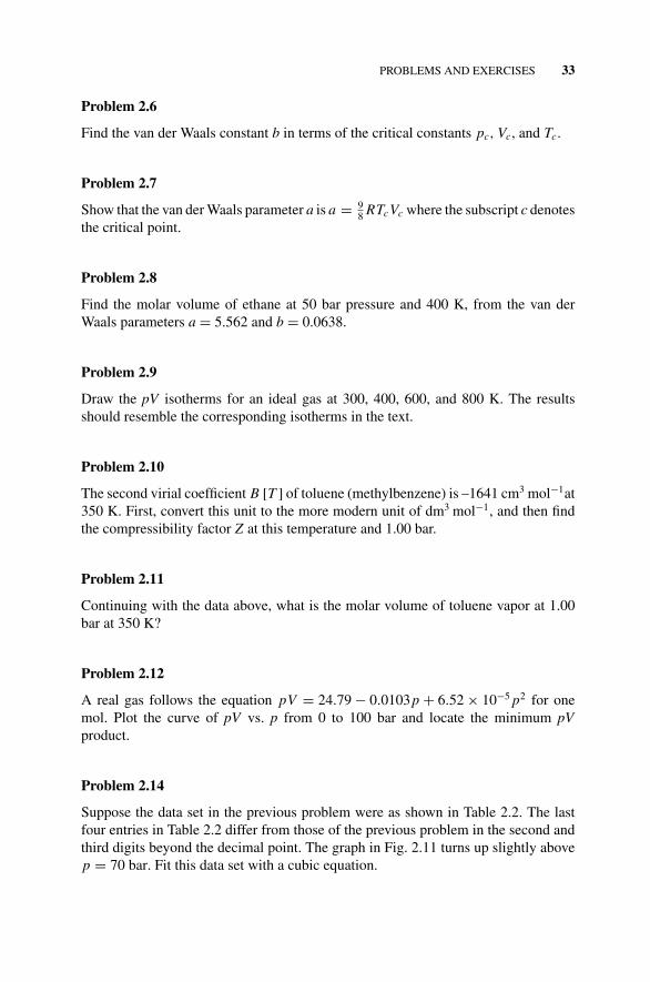
P1: OTA/XYZ P2: ABCc02 JWBS043-Rogers September 13, 2010 11:23 Printer Name: Yet to Come
PROBLEMS AND EXERCISES 33
Problem 2.6
Find the van der Waals constant b in terms of the critical constants pc, Vc, and Tc.
Problem 2.7
Show that the van der Waals parameter a is a = 98 RTcVc where the subscript c denotes
the critical point.
Problem 2.8
Find the molar volume of ethane at 50 bar pressure and 400 K, from the van derWaals parameters a = 5.562 and b = 0.0638.
Problem 2.9
Draw the pV isotherms for an ideal gas at 300, 400, 600, and 800 K. The resultsshould resemble the corresponding isotherms in the text.
Problem 2.10
The second virial coefficient B [T ] of toluene (methylbenzene) is –1641 cm3 mol−1at350 K. First, convert this unit to the more modern unit of dm3 mol−1, and then findthe compressibility factor Z at this temperature and 1.00 bar.
Problem 2.11
Continuing with the data above, what is the molar volume of toluene vapor at 1.00bar at 350 K?
Problem 2.12
A real gas follows the equation pV = 24.79 − 0.0103p + 6.52 × 10⁻⁵ p2 for onemol. Plot the curve of pV vs. p from 0 to 100 bar and locate the minimum pVproduct.
Problem 2.14
Suppose the data set in the previous problem were as shown in Table 2.2. The lastfour entries in Table 2.2 differ from those of the previous problem in the second andthird digits beyond the decimal point. The graph in Fig. 2.11 turns up slightly abovep = 70 bar. Fit this data set with a cubic equation.
P1: OTA/XYZ P2: ABCc02 JWBS043-Rogers September 13, 2010 11:23 Printer Name: Yet to Come
34 REAL GASES: EMPIRICAL EQUATIONS
p, bar
100806040200
pV
, dm
3 ba
r
24.3
24.4
24.5
24.6
24.7
24.8
FIGURE 2.11 Cubic real gas behavior.
Problem 2.15
(a) What is the volume of one mole of CO2 at 366 K and p = 111 bar accordingto the ideal gas law?
(b) The critical temperature of CO2 is 305.1 K. The critical pressure and volumeof CO2 are 73.8 bar and 0.0956 dm3(Laidler and Meiser, 1999). If a compress-ibility factor of 0.68 is read from a chart of isotherms, what is the reducedvolume of one mole of CO2 at 366 K and p = 111 bar according to the chart?
(c) The van der Waals parameters for CO2 are a = 3.66 and b = 0.0429. Whatis the volume of one mole of CO2 at 366 K and p = 111 bar according to thevan der Waals equation?
(d) What is the volume of one mole of CO2 at 366 K and p = 111 bar accordingto the corresponding states equation? What is the volume?
(e) The critical constants for helium are Tc = 5.3 K, pc = 2.29 bar, and Vc =0.0577 dm3 mol−1. What is the volume of one mole of He at 7.95 K andp = 2.75 bar according to the corresponding states equation? What is thevolume?

P1: OTA/XYZ P2: ABCc03 JWBS043-Rogers September 13, 2010 11:24 Printer Name: Yet to Come
3THE THERMODYNAMICSOF SIMPLE SYSTEMS
Thermodynamics, literally heat motion, is one of the pillars of physical chemistryand one of the great achievements of modern science. Classical thermodynamics isthe study of those quantities that are conserved, like energy, enthalpy, and free energy.Statistical thermodynamics is the link between this great theoretical edifice and thatof quantum mechanics.
3.1 CONSERVATION LAWS AND EXACT DIFFERENTIALS
Much of nineteenth-century thermodynamics was devoted to the discovery, definition,and characterization of physical quantities that are conserved. The simple statementenergy is conserved is one of the ways of stating the first law of thermodynamics.Conservation can be illustrated by carrying a rock up a hill and then bringing it backdown again. The potential energy of the rock in the gravitational field of the earthincreases on the way up and decreases on the way down, but it is the same at the endof the process as it was at the beginning; it is conserved. By contrast, work is notconserved. Carrying the rock around the circular path up and down the hill can beeasy or hard, depending on the path. Also, the work done on the way up is not thesame as the work that can be obtained by allowing the rock to drive some kind ofprimitive motor as it rolls down the hill.
Work is not the only factor that has to be taken into account. The difference betweenan easy path and a hard path up the hill is illustrated by the simplified model of amass being pushed up over the same change in height (altitude) but over two different
Concise Physical Chemistry, by Donald W. RogersCopyright C© 2011 John Wiley & Sons, Inc.
35
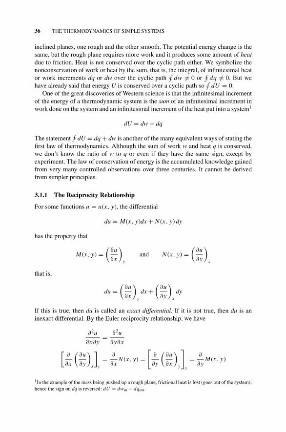
P1: OTA/XYZ P2: ABCc03 JWBS043-Rogers September 13, 2010 11:24 Printer Name: Yet to Come
36 THE THERMODYNAMICS OF SIMPLE SYSTEMS
inclined planes, one rough and the other smooth. The potential energy change is thesame, but the rough plane requires more work and it produces some amount of heatdue to friction. Heat is not conserved over the cyclic path either. We symbolize thenonconservation of work or heat by the sum, that is, the integral, of infinitesimal heator work increments dq or dw over the cyclic path
∮dw �= 0 or
∮dq �= 0. But we
have already said that energy U is conserved over a cyclic path so∮
dU = 0.One of the great discoveries of Western science is that the infinitesimal increment
of the energy of a thermodynamic system is the sum of an infinitesimal increment inwork done on the system and an infinitesimal increment of the heat put into a system1
dU = dw + dq
The statement∮
dU = dq + dw is another of the many equivalent ways of stating thefirst law of thermodynamics. Although the sum of work w and heat q is conserved,we don’t know the ratio of w to q or even if they have the same sign, except byexperiment. The law of conservation of energy is the accumulated knowledge gainedfrom very many controlled observations over three centuries. It cannot be derivedfrom simpler principles.
3.1.1 The Reciprocity Relationship
For some functions u = u(x, y), the differential
du = M(x, y)dx + N (x, y) dy
has the property that
M(x, y) =(
∂u
∂x
)y
and N (x, y) =(
∂u
∂y
)x
that is,
du =(
∂u
∂x
)y
dx +(
∂u
∂y
)x
dy
If this is true, then du is called an exact differential. If it is not true, then du is aninexact differential. By the Euler reciprocity relationship, we have
∂2u
∂x∂y= ∂2u
∂y∂x[
∂
∂x
(∂u
∂y
)x
]y
= ∂
∂xN (x, y) =
[∂
∂y
(∂u
∂x
)y
]x
= ∂
∂yM(x, y)
1In the example of the mass being pushed up a rough plane, frictional heat is lost (goes out of the system);hence the sign on dq is reversed: dU = dw in − dqout.
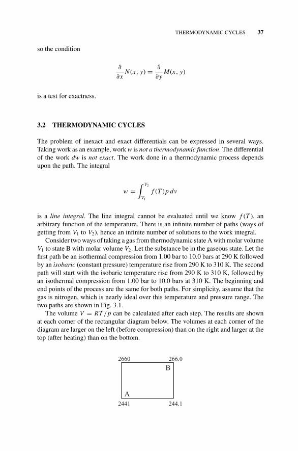
P1: OTA/XYZ P2: ABCc03 JWBS043-Rogers September 13, 2010 11:24 Printer Name: Yet to Come
THERMODYNAMIC CYCLES 37
so the condition
∂
∂xN (x, y) = ∂
∂yM(x, y)
is a test for exactness.
3.2 THERMODYNAMIC CYCLES
The problem of inexact and exact differentials can be expressed in several ways.Taking work as an example, work w is not a thermodynamic function. The differentialof the work dw is not exact. The work done in a thermodynamic process dependsupon the path. The integral
w =∫ V2
V1
f (T )p dv
is a line integral. The line integral cannot be evaluated until we know f (T ), anarbitrary function of the temperature. There is an infinite number of paths (ways ofgetting from V1 to V2), hence an infinite number of solutions to the work integral.
Consider two ways of taking a gas from thermodynamic state A with molar volumeV1 to state B with molar volume V2. Let the substance be in the gaseous state. Let thefirst path be an isothermal compression from 1.00 bar to 10.0 bars at 290 K followedby an isobaric (constant pressure) temperature rise from 290 K to 310 K. The secondpath will start with the isobaric temperature rise from 290 K to 310 K, followed byan isothermal compression from 1.00 bar to 10.0 bars at 310 K. The beginning andend points of the process are the same for both paths. For simplicity, assume that thegas is nitrogen, which is nearly ideal over this temperature and pressure range. Thetwo paths are shown in Fig. 3.1.
The volume V = RT /p can be calculated after each step. The results are shownat each corner of the rectangular diagram below. The volumes at each corner of thediagram are larger on the left (before compression) than on the right and larger at thetop (after heating) than on the bottom.
2441 244.1
2660 266.0
A
B
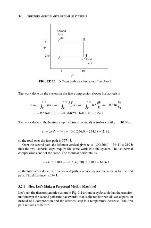
P1: OTA/XYZ P2: ABCc03 JWBS043-Rogers September 13, 2010 11:24 Printer Name: Yet to Come
38 THE THERMODYNAMICS OF SIMPLE SYSTEMS
FirstPath
SecondPath
T
p1 10
290
310
A
B
FIGURE 3.1 Different path transformations from A to B.
The work done on the system in the first compression (lower horizontal) is
w = −∫ V2
V1
p dV = −∫ V2
V1
RT
VdV = −
∫ V2
V1
RTdV
V= −RT ln
V2
V1
= −RT ln 0.100 = −8.314(290) ln 0.100 = 5552 J
The work done in the heating step (rightmost vertical) is isobaric with p = 10.0 bar:
w = p(V2 − V1) = 10.0 (266.0 − 244.1) = 219 J
so the total over the first path is 5771 J.Over the second path, the leftmost vertical gives w = 1.00(2660 − 2441) = 219 J;
thus the two isobaric steps require the same work into the system. The isothermalcompressions are not the same. The topmost horizontal is
−RT ln 0.100 = −8.314(320) ln 0.100 = 6126 J
so the total work done over the second path is obviously not the same as by the firstpath. The difference is 574 J.
3.2.1 Hey, Let’s Make a Perpetual Motion Machine!
Let’s run the thermodynamic system in Fig. 3.1 around a cycle such that the transfor-mation over the second path runs backwards; that is, the top horizontal is an expansioninstead of a compression and the leftmost step is a temperature decrease. The firstpath remains as before.
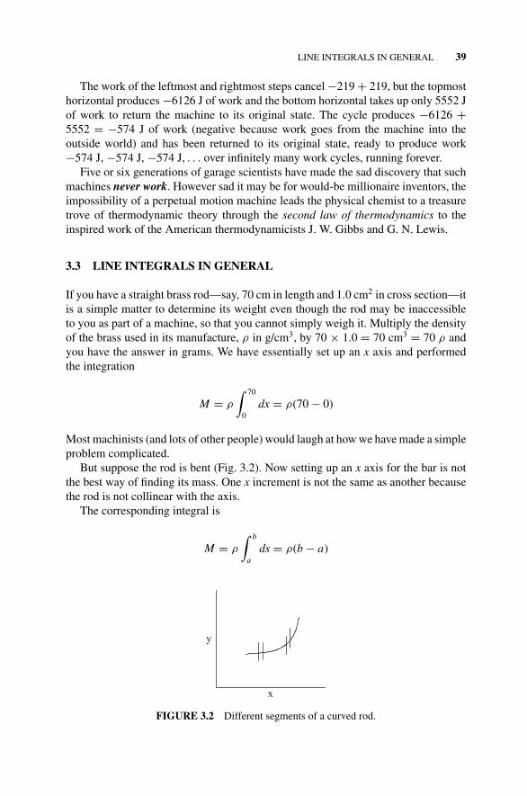
P1: OTA/XYZ P2: ABCc03 JWBS043-Rogers September 13, 2010 11:24 Printer Name: Yet to Come
LINE INTEGRALS IN GENERAL 39
The work of the leftmost and rightmost steps cancel −219 + 219, but the topmosthorizontal produces −6126 J of work and the bottom horizontal takes up only 5552 Jof work to return the machine to its original state. The cycle produces −6126 +5552 = −574 J of work (negative because work goes from the machine into theoutside world) and has been returned to its original state, ready to produce work−574 J, −574 J, −574 J, . . . over infinitely many work cycles, running forever.
Five or six generations of garage scientists have made the sad discovery that suchmachines never work. However sad it may be for would-be millionaire inventors, theimpossibility of a perpetual motion machine leads the physical chemist to a treasuretrove of thermodynamic theory through the second law of thermodynamics to theinspired work of the American thermodynamicists J. W. Gibbs and G. N. Lewis.
3.3 LINE INTEGRALS IN GENERAL
If you have a straight brass rod—say, 70 cm in length and 1.0 cm2 in cross section—itis a simple matter to determine its weight even though the rod may be inaccessibleto you as part of a machine, so that you cannot simply weigh it. Multiply the densityof the brass used in its manufacture, ρ in g/cm3, by 70 × 1.0 = 70 cm3 = 70 ρ andyou have the answer in grams. We have essentially set up an x axis and performedthe integration
M = ρ
∫ 70
0dx = ρ(70 − 0)
Most machinists (and lots of other people) would laugh at how we have made a simpleproblem complicated.
But suppose the rod is bent (Fig. 3.2). Now setting up an x axis for the bar is notthe best way of finding its mass. One x increment is not the same as another becausethe rod is not collinear with the axis.
The corresponding integral is
M = ρ
∫ b
ads = ρ(b − a)
y
x
FIGURE 3.2 Different segments of a curved rod.
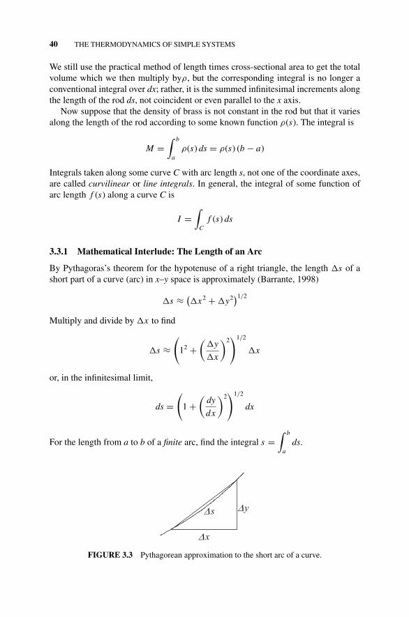
P1: OTA/XYZ P2: ABCc03 JWBS043-Rogers September 13, 2010 11:24 Printer Name: Yet to Come
40 THE THERMODYNAMICS OF SIMPLE SYSTEMS
We still use the practical method of length times cross-sectional area to get the totalvolume which we then multiply byρ, but the corresponding integral is no longer aconventional integral over dx; rather, it is the summed infinitesimal increments alongthe length of the rod ds, not coincident or even parallel to the x axis.
Now suppose that the density of brass is not constant in the rod but that it variesalong the length of the rod according to some known function ρ(s). The integral is
M =∫ b
aρ(s) ds = ρ(s) (b − a)
Integrals taken along some curve C with arc length s, not one of the coordinate axes,are called curvilinear or line integrals. In general, the integral of some function ofarc length f (s) along a curve C is
I =∫
Cf (s) ds
3.3.1 Mathematical Interlude: The Length of an Arc
By Pythagoras’s theorem for the hypotenuse of a right triangle, the length �s of ashort part of a curve (arc) in x–y space is approximately (Barrante, 1998)
�s ≈ (�x2 + �y2
)1/2
Multiply and divide by �x to find
�s ≈(
12 +(
�y
�x
)2)1/2
�x
or, in the infinitesimal limit,
ds =(
1 +(
dy
dx
)2)1/2
dx
For the length from a to b of a finite arc, find the integral s =∫ b
ads.
s
x
y
FIGURE 3.3 Pythagorean approximation to the short arc of a curve.
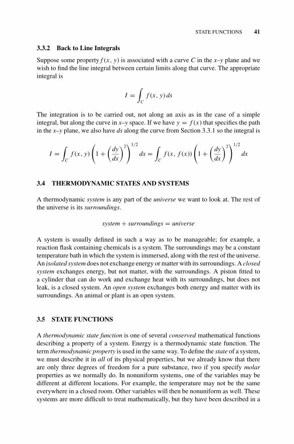
P1: OTA/XYZ P2: ABCc03 JWBS043-Rogers September 13, 2010 11:24 Printer Name: Yet to Come
STATE FUNCTIONS 41
3.3.2 Back to Line Integrals
Suppose some property f (x, y) is associated with a curve C in the x–y plane and wewish to find the line integral between certain limits along that curve. The appropriateintegral is
I =∫
Cf (x, y) ds
The integration is to be carried out, not along an axis as in the case of a simpleintegral, but along the curve in x–y space. If we have y = f (x) that specifies the pathin the x–y plane, we also have ds along the curve from Section 3.3.1 so the integral is
I =∫
Cf (x, y)
(1 +
(dy
dx
)2)1/2
dx =∫
Cf (x, f (x))
(1 +
(dy
dx
)2)1/2
dx
3.4 THERMODYNAMIC STATES AND SYSTEMS
A thermodynamic system is any part of the universe we want to look at. The rest ofthe universe is its surroundings.
system + surroundings = universe
A system is usually defined in such a way as to be manageable; for example, areaction flask containing chemicals is a system. The surroundings may be a constanttemperature bath in which the system is immersed, along with the rest of the universe.An isolated system does not exchange energy or matter with its surroundings. A closedsystem exchanges energy, but not matter, with the surroundings. A piston fitted toa cylinder that can do work and exchange heat with its surroundings, but does notleak, is a closed system. An open system exchanges both energy and matter with itssurroundings. An animal or plant is an open system.
3.5 STATE FUNCTIONS
A thermodynamic state function is one of several conserved mathematical functionsdescribing a property of a system. Energy is a thermodynamic state function. Theterm thermodynamic property is used in the same way. To define the state of a system,we must describe it in all of its physical properties, but we already know that thereare only three degrees of freedom for a pure substance, two if you specify molarproperties as we normally do. In nonuniform systems, one of the variables may bedifferent at different locations. For example, the temperature may not be the sameeverywhere in a closed room. Other variables will then be nonuniform as well. Thesesystems are more difficult to treat mathematically, but they have been described in a
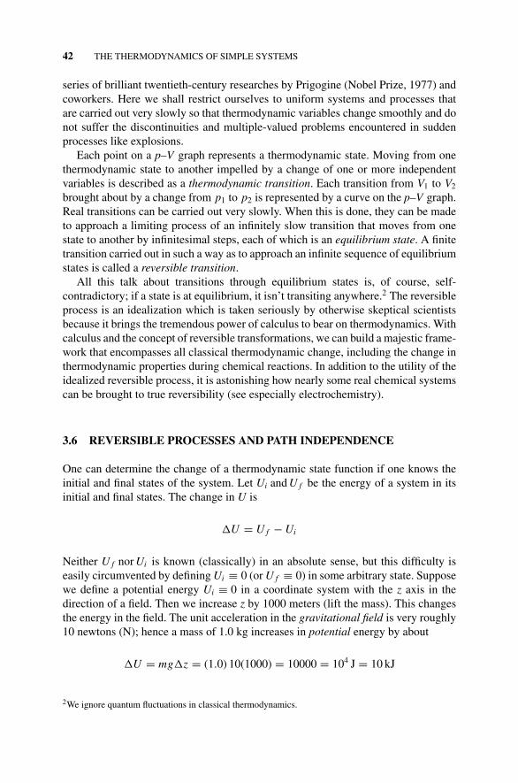
P1: OTA/XYZ P2: ABCc03 JWBS043-Rogers September 13, 2010 11:24 Printer Name: Yet to Come
42 THE THERMODYNAMICS OF SIMPLE SYSTEMS
series of brilliant twentieth-century researches by Prigogine (Nobel Prize, 1977) andcoworkers. Here we shall restrict ourselves to uniform systems and processes thatare carried out very slowly so that thermodynamic variables change smoothly and donot suffer the discontinuities and multiple-valued problems encountered in suddenprocesses like explosions.
Each point on a p–V graph represents a thermodynamic state. Moving from onethermodynamic state to another impelled by a change of one or more independentvariables is described as a thermodynamic transition. Each transition from V1 to V2
brought about by a change from p1 to p2 is represented by a curve on the p–V graph.Real transitions can be carried out very slowly. When this is done, they can be madeto approach a limiting process of an infinitely slow transition that moves from onestate to another by infinitesimal steps, each of which is an equilibrium state. A finitetransition carried out in such a way as to approach an infinite sequence of equilibriumstates is called a reversible transition.
All this talk about transitions through equilibrium states is, of course, self-contradictory; if a state is at equilibrium, it isn’t transiting anywhere.2 The reversibleprocess is an idealization which is taken seriously by otherwise skeptical scientistsbecause it brings the tremendous power of calculus to bear on thermodynamics. Withcalculus and the concept of reversible transformations, we can build a majestic frame-work that encompasses all classical thermodynamic change, including the change inthermodynamic properties during chemical reactions. In addition to the utility of theidealized reversible process, it is astonishing how nearly some real chemical systemscan be brought to true reversibility (see especially electrochemistry).
3.6 REVERSIBLE PROCESSES AND PATH INDEPENDENCE
One can determine the change of a thermodynamic state function if one knows theinitial and final states of the system. Let Ui and U f be the energy of a system in itsinitial and final states. The change in U is
�U = U f − Ui
Neither U f nor Ui is known (classically) in an absolute sense, but this difficulty iseasily circumvented by defining Ui ≡ 0 (or U f ≡ 0) in some arbitrary state. Supposewe define a potential energy Ui ≡ 0 in a coordinate system with the z axis in thedirection of a field. Then we increase z by 1000 meters (lift the mass). This changesthe energy in the field. The unit acceleration in the gravitational field is very roughly10 newtons (N); hence a mass of 1.0 kg increases in potential energy by about
�U = mg�z = (1.0) 10(1000) = 10000 = 104 J = 10 kJ
2We ignore quantum fluctuations in classical thermodynamics.
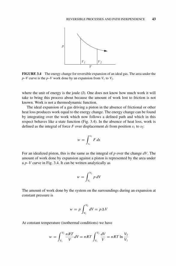
P1: OTA/XYZ P2: ABCc03 JWBS043-Rogers September 13, 2010 11:24 Printer Name: Yet to Come
REVERSIBLE PROCESSES AND PATH INDEPENDENCE 43
p
VV1 V2
FIGURE 3.4 The energy change for reversible expansion of an ideal gas. The area under thep–V curve is the p–V work done by an expansion from V1 to V2.
where the unit of energy is the joule (J). One does not know how much work it willtake to bring this process about because the amount of work lost to friction is notknown. Work is not a thermodynamic function.
The ideal expansion of a gas driving a piston in the absence of frictional or otherheat loss produces work equal to the energy change. The energy change can be foundby integrating over the work which now follows a defined path and which in thisrespect behaves like a state function (Fig. 3.4). In the absence of heat loss, work isdefined as the integral of force F over displacement ds from position s1 to s2:
w =∫ s2
s1
F ds
For an idealized piston, this is the same as the integral of p over the change dV . Theamount of work done by expansion against a piston is represented by the area undera p–V curve in Fig. 3.4. It can be written analytically as
w =∫ V2
V1
p dV
The amount of work done by the system on the surroundings during an expansion atconstant pressure is
w = p∫ V2
V1
dV = p�V
At constant temperature (isothermal conditions) we have
w =∫ V2
V1
n RT
VdV = n RT
∫ V2
V1
dV
V= n RT ln
V2
V1
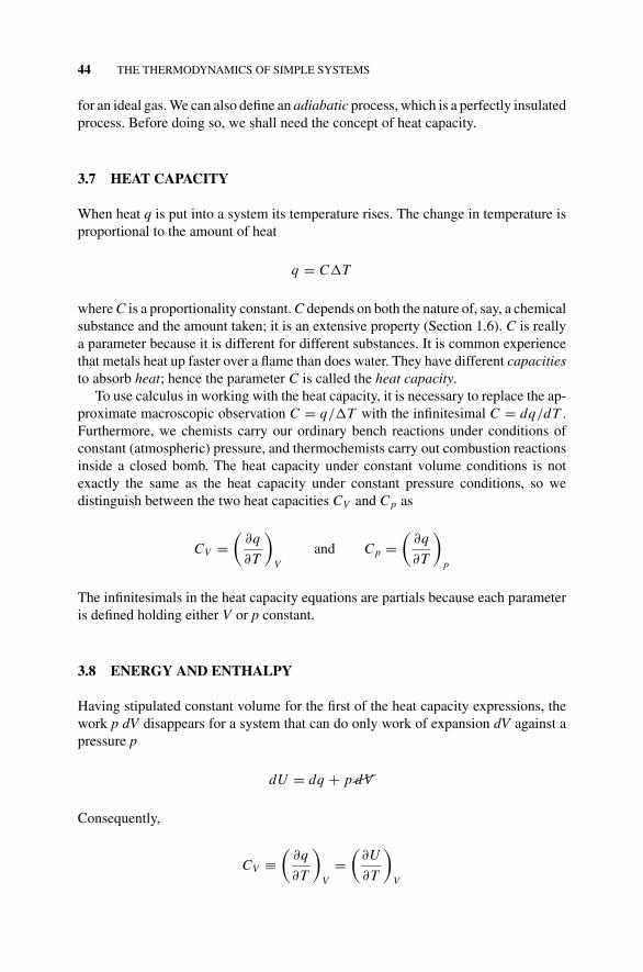
P1: OTA/XYZ P2: ABCc03 JWBS043-Rogers September 13, 2010 11:24 Printer Name: Yet to Come
44 THE THERMODYNAMICS OF SIMPLE SYSTEMS
for an ideal gas. We can also define an adiabatic process, which is a perfectly insulatedprocess. Before doing so, we shall need the concept of heat capacity.
3.7 HEAT CAPACITY
When heat q is put into a system its temperature rises. The change in temperature isproportional to the amount of heat
q = C�T
where C is a proportionality constant. C depends on both the nature of, say, a chemicalsubstance and the amount taken; it is an extensive property (Section 1.6). C is reallya parameter because it is different for different substances. It is common experiencethat metals heat up faster over a flame than does water. They have different capacitiesto absorb heat; hence the parameter C is called the heat capacity.
To use calculus in working with the heat capacity, it is necessary to replace the ap-proximate macroscopic observation C = q/�T with the infinitesimal C = dq/dT .Furthermore, we chemists carry our ordinary bench reactions under conditions ofconstant (atmospheric) pressure, and thermochemists carry out combustion reactionsinside a closed bomb. The heat capacity under constant volume conditions is notexactly the same as the heat capacity under constant pressure conditions, so wedistinguish between the two heat capacities CV and C p as
CV =(
∂q
∂T
)V
and C p =(
∂q
∂T
)p
The infinitesimals in the heat capacity equations are partials because each parameteris defined holding either V or p constant.
3.8 ENERGY AND ENTHALPY
Having stipulated constant volume for the first of the heat capacity expressions, thework p dV disappears for a system that can do only work of expansion dV against apressure p
dU = dq + p dV
Consequently,
CV ≡(
∂q
∂T
)V
=(
∂U
∂T
)V
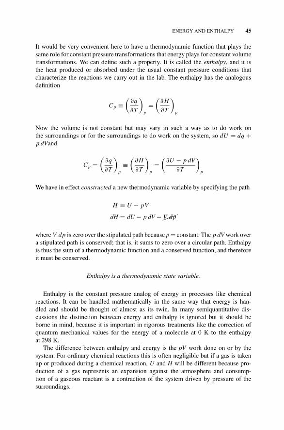
P1: OTA/XYZ P2: ABCc03 JWBS043-Rogers September 13, 2010 11:24 Printer Name: Yet to Come
ENERGY AND ENTHALPY 45
It would be very convenient here to have a thermodynamic function that plays thesame role for constant pressure transformations that energy plays for constant volumetransformations. We can define such a property. It is called the enthalpy, and it isthe heat produced or absorbed under the usual constant pressure conditions thatcharacterize the reactions we carry out in the lab. The enthalpy has the analogousdefinition
C p ≡(
∂q
∂T
)p
=(
∂ H
∂T
)p
Now the volume is not constant but may vary in such a way as to do work onthe surroundings or for the surroundings to do work on the system, so dU = dq +p dVand
C p =(
∂q
∂T
)p
≡(
∂ H
∂T
)p
=(
∂U − p dV
∂T
)p
We have in effect constructed a new thermodynamic variable by specifying the path
H ≡ U − pV
dH = dU − p dV − V dp
where V dp is zero over the stipulated path because p = constant. The p dV work overa stipulated path is conserved; that is, it sums to zero over a circular path. Enthalpyis thus the sum of a thermodynamic function and a conserved function, and thereforeit must be conserved.
Enthalpy is a thermodynamic state variable.
Enthalpy is the constant pressure analog of energy in processes like chemicalreactions. It can be handled mathematically in the same way that energy is han-dled and should be thought of almost as its twin. In many semiquantitative dis-cussions the distinction between energy and enthalpy is ignored but it should beborne in mind, because it is important in rigorous treatments like the correction ofquantum mechanical values for the energy of a molecule at 0 K to the enthalpyat 298 K.
The difference between enthalpy and energy is the pV work done on or by thesystem. For ordinary chemical reactions this is often negligible but if a gas is takenup or produced during a chemical reaction, U and H will be different because pro-duction of a gas represents an expansion against the atmosphere and consump-tion of a gaseous reactant is a contraction of the system driven by pressure of thesurroundings.
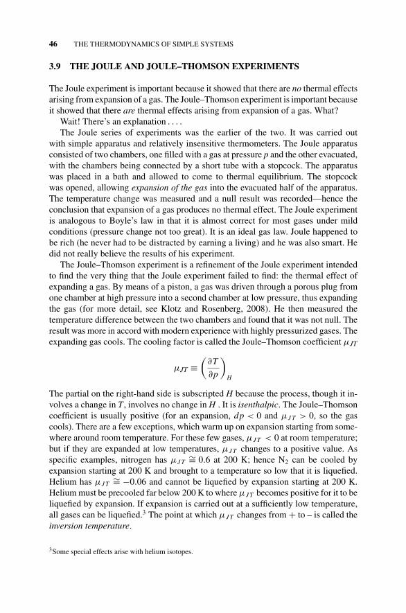
P1: OTA/XYZ P2: ABCc03 JWBS043-Rogers September 13, 2010 11:24 Printer Name: Yet to Come
46 THE THERMODYNAMICS OF SIMPLE SYSTEMS
3.9 THE JOULE AND JOULE–THOMSON EXPERIMENTS
The Joule experiment is important because it showed that there are no thermal effectsarising from expansion of a gas. The Joule–Thomson experiment is important becauseit showed that there are thermal effects arising from expansion of a gas. What?
Wait! There’s an explanation . . . .The Joule series of experiments was the earlier of the two. It was carried out
with simple apparatus and relatively insensitive thermometers. The Joule apparatusconsisted of two chambers, one filled with a gas at pressure p and the other evacuated,with the chambers being connected by a short tube with a stopcock. The apparatuswas placed in a bath and allowed to come to thermal equilibrium. The stopcockwas opened, allowing expansion of the gas into the evacuated half of the apparatus.The temperature change was measured and a null result was recorded—hence theconclusion that expansion of a gas produces no thermal effect. The Joule experimentis analogous to Boyle’s law in that it is almost correct for most gases under mildconditions (pressure change not too great). It is an ideal gas law. Joule happened tobe rich (he never had to be distracted by earning a living) and he was also smart. Hedid not really believe the results of his experiment.
The Joule–Thomson experiment is a refinement of the Joule experiment intendedto find the very thing that the Joule experiment failed to find: the thermal effect ofexpanding a gas. By means of a piston, a gas was driven through a porous plug fromone chamber at high pressure into a second chamber at low pressure, thus expandingthe gas (for more detail, see Klotz and Rosenberg, 2008). He then measured thetemperature difference between the two chambers and found that it was not null. Theresult was more in accord with modern experience with highly pressurized gases. Theexpanding gas cools. The cooling factor is called the Joule–Thomson coefficient µJT
µJT ≡(
∂T
∂p
)H
The partial on the right-hand side is subscripted H because the process, though it in-volves a change in T , involves no change in H . It is isenthalpic. The Joule–Thomsoncoefficient is usually positive (for an expansion, dp < 0 and µJ T > 0, so the gascools). There are a few exceptions, which warm up on expansion starting from some-where around room temperature. For these few gases, µJ T < 0 at room temperature;but if they are expanded at low temperatures, µJ T changes to a positive value. Asspecific examples, nitrogen has µJ T
∼= 0.6 at 200 K; hence N2 can be cooled byexpansion starting at 200 K and brought to a temperature so low that it is liquefied.Helium has µJ T
∼= −0.06 and cannot be liquefied by expansion starting at 200 K.Helium must be precooled far below 200 K to where µJ T becomes positive for it to beliquefied by expansion. If expansion is carried out at a sufficiently low temperature,all gases can be liquefied.3 The point at which µJ T changes from + to – is called theinversion temperature.
3Some special effects arise with helium isotopes.
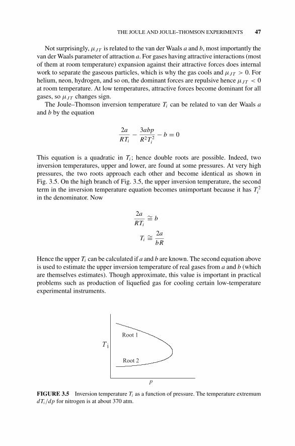
P1: OTA/XYZ P2: ABCc03 JWBS043-Rogers September 13, 2010 11:24 Printer Name: Yet to Come
THE JOULE AND JOULE–THOMSON EXPERIMENTS 47
Not surprisingly, µJ T is related to the van der Waals a and b, most importantly thevan der Waals parameter of attraction a. For gases having attractive interactions (mostof them at room temperature) expansion against their attractive forces does internalwork to separate the gaseous particles, which is why the gas cools and µJ T > 0. Forhelium, neon, hydrogen, and so on, the dominant forces are repulsive hence µJ T < 0at room temperature. At low temperatures, attractive forces become dominant for allgases, so µJ T changes sign.
The Joule–Thomson inversion temperature Ti can be related to van der Waals aand b by the equation
2a
RTi− 3abp
R2T 2i
− b = 0
This equation is a quadratic in Ti ; hence double roots are possible. Indeed, twoinversion temperatures, upper and lower, are found at some pressures. At very highpressures, the two roots approach each other and become identical as shown inFig. 3.5. On the high branch of Fig. 3.5, the upper inversion temperature, the secondterm in the inversion temperature equation becomes unimportant because it has T 2
iin the denominator. Now
2a
RTi
∼= b
Ti∼= 2a
bR
Hence the upper Ti can be calculated if a and b are known. The second equation aboveis used to estimate the upper inversion temperature of real gases from a and b (whichare themselves estimates). Though approximate, this value is important in practicalproblems such as production of liquefied gas for cooling certain low-temperatureexperimental instruments.
T i
p
Root 1
Root 2
FIGURE 3.5 Inversion temperature Ti as a function of pressure. The temperature extremumdTi/dp for nitrogen is at about 370 atm.
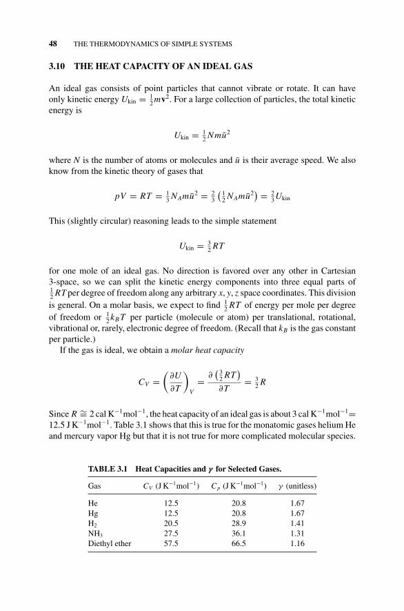
P1: OTA/XYZ P2: ABCc03 JWBS043-Rogers September 13, 2010 11:24 Printer Name: Yet to Come
48 THE THERMODYNAMICS OF SIMPLE SYSTEMS
3.10 THE HEAT CAPACITY OF AN IDEAL GAS
An ideal gas consists of point particles that cannot vibrate or rotate. It can haveonly kinetic energy Ukin = 1
2 mv2. For a large collection of particles, the total kineticenergy is
Ukin = 12 Nmu2
where N is the number of atoms or molecules and u is their average speed. We alsoknow from the kinetic theory of gases that
pV = RT = 13 NAmu2 = 2
3
(12 NAmu2
) = 23Ukin
This (slightly circular) reasoning leads to the simple statement
Ukin = 32 RT
for one mole of an ideal gas. No direction is favored over any other in Cartesian3-space, so we can split the kinetic energy components into three equal parts of12 RT per degree of freedom along any arbitrary x, y, z space coordinates. This divisionis general. On a molar basis, we expect to find 1
2 RT of energy per mole per degreeof freedom or 1
2 kB T per particle (molecule or atom) per translational, rotational,vibrational or, rarely, electronic degree of freedom. (Recall that kB is the gas constantper particle.)
If the gas is ideal, we obtain a molar heat capacity
CV =(
∂U
∂T
)V
= ∂(
32 RT
)∂T
= 32 R
Since R ∼= 2 cal K−1mol−1, the heat capacity of an ideal gas is about 3 cal K−1mol−1=12.5 J K−1mol−1. Table 3.1 shows that this is true for the monatomic gases helium Heand mercury vapor Hg but that it is not true for more complicated molecular species.
TABLE 3.1 Heat Capacities and γ for Selected Gases.
Gas CV (J K−1mol−1) Cp (J K−1mol−1) γ (unitless)
He 12.5 20.8 1.67Hg 12.5 20.8 1.67H2 20.5 28.9 1.41NH3 27.5 36.1 1.31Diethyl ether 57.5 66.5 1.16
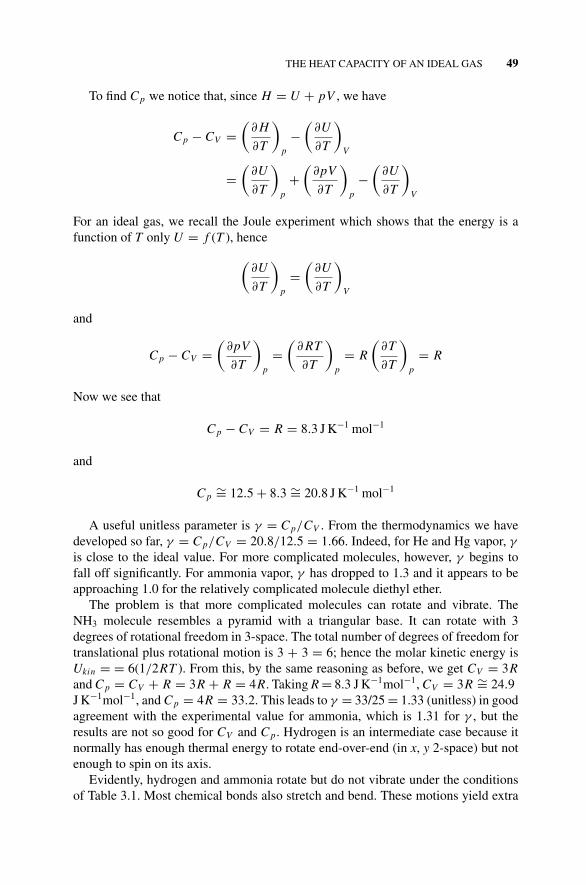
P1: OTA/XYZ P2: ABCc03 JWBS043-Rogers September 13, 2010 11:24 Printer Name: Yet to Come
THE HEAT CAPACITY OF AN IDEAL GAS 49
To find C p we notice that, since H = U + pV , we have
C p − CV =(
∂ H
∂T
)p
−(
∂U
∂T
)V
=(
∂U
∂T
)p
+(
∂pV
∂T
)p
−(
∂U
∂T
)V
For an ideal gas, we recall the Joule experiment which shows that the energy is afunction of T only U = f (T ), hence
(∂U
∂T
)p
=(
∂U
∂T
)V
and
C p − CV =(
∂pV
∂T
)p
=(
∂ RT
∂T
)p
= R
(∂T
∂T
)p
= R
Now we see that
C p − CV = R = 8.3 J K−1 mol−1
and
C p∼= 12.5 + 8.3 ∼= 20.8 J K−1 mol−1
A useful unitless parameter is γ = C p/CV . From the thermodynamics we havedeveloped so far, γ = C p/CV = 20.8/12.5 = 1.66. Indeed, for He and Hg vapor, γ
is close to the ideal value. For more complicated molecules, however, γ begins tofall off significantly. For ammonia vapor, γ has dropped to 1.3 and it appears to beapproaching 1.0 for the relatively complicated molecule diethyl ether.
The problem is that more complicated molecules can rotate and vibrate. TheNH3 molecule resembles a pyramid with a triangular base. It can rotate with 3degrees of rotational freedom in 3-space. The total number of degrees of freedom fortranslational plus rotational motion is 3 + 3 = 6; hence the molar kinetic energy isUkin = = 6(1/2RT ). From this, by the same reasoning as before, we get CV = 3Rand C p = CV + R = 3R + R = 4R. Taking R = 8.3 J K−1mol−1, CV = 3R ∼= 24.9J K−1mol−1, and C p = 4R = 33.2. This leads to γ = 33/25 = 1.33 (unitless) in goodagreement with the experimental value for ammonia, which is 1.31 for γ , but theresults are not so good for CV and C p. Hydrogen is an intermediate case because itnormally has enough thermal energy to rotate end-over-end (in x, y 2-space) but notenough to spin on its axis.
Evidently, hydrogen and ammonia rotate but do not vibrate under the conditionsof Table 3.1. Most chemical bonds also stretch and bend. These motions yield extra
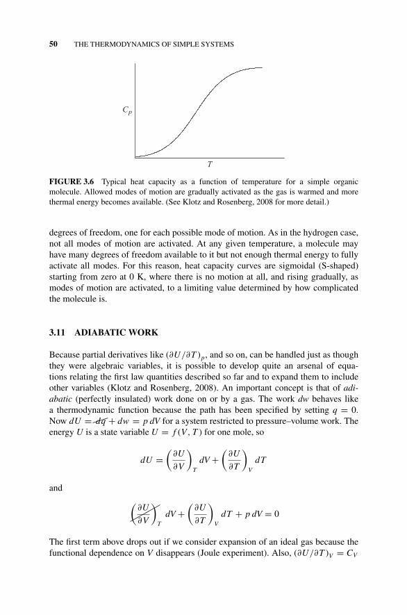
P1: OTA/XYZ P2: ABCc03 JWBS043-Rogers September 13, 2010 11:24 Printer Name: Yet to Come
50 THE THERMODYNAMICS OF SIMPLE SYSTEMS
Cp
T
FIGURE 3.6 Typical heat capacity as a function of temperature for a simple organicmolecule. Allowed modes of motion are gradually activated as the gas is warmed and morethermal energy becomes available. (See Klotz and Rosenberg, 2008 for more detail.)
degrees of freedom, one for each possible mode of motion. As in the hydrogen case,not all modes of motion are activated. At any given temperature, a molecule mayhave many degrees of freedom available to it but not enough thermal energy to fullyactivate all modes. For this reason, heat capacity curves are sigmoidal (S-shaped)starting from zero at 0 K, where there is no motion at all, and rising gradually, asmodes of motion are activated, to a limiting value determined by how complicatedthe molecule is.
3.11 ADIABATIC WORK
Because partial derivatives like (∂U/∂T )p, and so on, can be handled just as thoughthey were algebraic variables, it is possible to develop quite an arsenal of equa-tions relating the first law quantities described so far and to expand them to includeother variables (Klotz and Rosenberg, 2008). An important concept is that of adi-abatic (perfectly insulated) work done on or by a gas. The work dw behaves likea thermodynamic function because the path has been specified by setting q = 0.Now dU = dq + dw = p dV for a system restricted to pressure–volume work. Theenergy U is a state variable U = f (V, T ) for one mole, so
dU =(
∂U
∂V
)T
dV +(
∂U
∂T
)V
dT
and
(∂U
∂V
)T
dV +(
∂U
∂T
)V
dT + p dV = 0
The first term above drops out if we consider expansion of an ideal gas because thefunctional dependence on V disappears (Joule experiment). Also, (∂U/∂T )V = CV
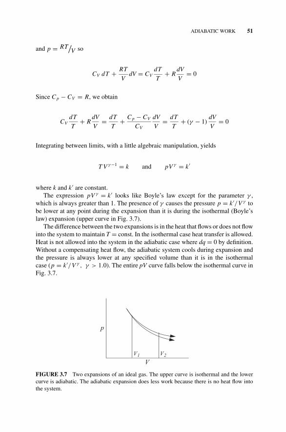
P1: OTA/XYZ P2: ABCc03 JWBS043-Rogers September 13, 2010 11:24 Printer Name: Yet to Come
ADIABATIC WORK 51
and p = RT/V so
CV dT + RT
VdV = CV
dT
T+ R
dV
V= 0
Since C p − CV = R, we obtain
CVdT
T+ R
dV
V= dT
T+ C p − CV
CV
dV
V= dT
T+ (γ − 1)
dV
V= 0
Integrating between limits, with a little algebraic manipulation, yields
T V γ−1 = k and pV γ = k ′
where k and k ′ are constant.The expression pV γ = k ′ looks like Boyle’s law except for the parameter γ ,
which is always greater than 1. The presence of γ causes the pressure p = k ′/V γ tobe lower at any point during the expansion than it is during the isothermal (Boyle’slaw) expansion (upper curve in Fig. 3.7).
The difference between the two expansions is in the heat that flows or does not flowinto the system to maintain T = const. In the isothermal case heat transfer is allowed.Heat is not allowed into the system in the adiabatic case where dq = 0 by definition.Without a compensating heat flow, the adiabatic system cools during expansion andthe pressure is always lower at any specified volume than it is in the isothermalcase (p = k ′/V γ , γ > 1.0). The entire pV curve falls below the isothermal curve inFig. 3.7.
p
VV1 V2
FIGURE 3.7 Two expansions of an ideal gas. The upper curve is isothermal and the lowercurve is adiabatic. The adiabatic expansion does less work because there is no heat flow intothe system.
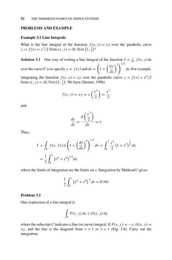
P1: OTA/XYZ P2: ABCc03 JWBS043-Rogers September 13, 2010 11:24 Printer Name: Yet to Come
52 THE THERMODYNAMICS OF SIMPLE SYSTEMS
PROBLEMS AND EXAMPLE
Example 3.1 Line Integrals
What is the line integral of the function f (x, y) = xy over the parabolic curvey = f (x) = x2/2 from (x, y) = (0, 0) to
(1, 1
2
)?
Solution 3.1 One way of writing a line integral of the function I = ∫C f (x, y) ds
over the curve C is to specify y = f (x) and ds =(
1 +(
dy
dx
)2)1/2
dx. For example,
integrating the function f (x, y) = xy over the parabolic curve y = f (x) = x2/2from (x, y) = (0, 0) to
(1, 1
2
). We have (Steiner, 1996)
f (x, y) = xy = x
(x2
2
)= x3
2
and
dy
dx=
d
(x2
2
)
dx= x
Thus,
I =∫
Cf (x, f (x))
(1 +
(dy
dx
)2)1/2
dx =∫ 1
0
x3
2
(1 + x2
) 12 dx
= 1
2
∫ 1
0
(x6 + x8)1/2
dx
where the limits of integration are the limits on x. Integration by Mathcad C© gives
1
2
∫ 1
0
(x6 + x8
).5dx = 0.161
Problem 3.1
One expression of a line integral is
∫C
F(x, y) dx + G(x, y) dy
where the subscript C indicates a line (or curve) integral. If F(x, y) = −y, G(x, y) =xy, and the line is the diagonal from x = 1 to y = 1 (Fig. 3.8). Carry out theintegration.
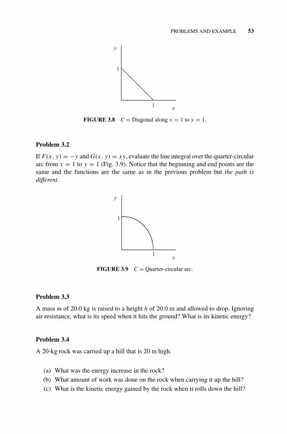
P1: OTA/XYZ P2: ABCc03 JWBS043-Rogers September 13, 2010 11:24 Printer Name: Yet to Come
PROBLEMS AND EXAMPLE 53
y
x
1
1
FIGURE 3.8 C = Diagonal along x = 1 to y = 1.
Problem 3.2
If F(x, y) = −y and G(x, y) = xy, evaluate the line integral over the quarter-circulararc from x = 1 to y = 1 (Fig. 3.9). Notice that the beginning and end points are thesame and the functions are the same as in the previous problem but the path isdifferent.
y
x
1
1
FIGURE 3.9 C = Quarter-circular arc.
Problem 3.3
A mass m of 20.0 kg is raised to a height h of 20.0 m and allowed to drop. Ignoringair resistance, what is its speed when it hits the ground? What is its kinetic energy?
Problem 3.4
A 20-kg rock was carried up a hill that is 20 m high.
(a) What was the energy increase in the rock?
(b) What amount of work was done on the rock when carrying it up the hill?
(c) What is the kinetic energy gained by the rock when it rolls down the hill?

P1: OTA/XYZ P2: ABCc03 JWBS043-Rogers September 13, 2010 11:24 Printer Name: Yet to Come
54 THE THERMODYNAMICS OF SIMPLE SYSTEMS
Problem 3.5
In a Joule experiment, two 20.3-kg weights fell 1.524 m to drive a paddle wheelimmersed in 6.31 kg of water. The experiment was repeated 20 times, after whichthe temperature of the water bath was found to have risen by 0.352 K. What is themechanical equivalent of heat in J K−1 according to this experiment?
Problem 3.6
Show that dw is an inexact differential for one mole of an ideal gas undergoing areversible expansion.
Problem 3.7
The definition of the calorie is that amount of heat that is necessary to raise 1 g ofwater 1 K. As it stands, this definition is approximately valid for temperature changesnot too far from room temperature. Use this approximate definition to predict thefinal temperature of 200 g of water at 283 K mixed with 450 g of water at 350 K.
Problem 3.8
Show that, for an ideal gas with constant CV , we have
T2
T1=
(V1
V2
) RCV
Problem 3.9
From the kinetic theory of gases, we get the expression U = 32 RT for the energy of
an ideal monatomic gas. Show that dU is an exact differential.
Problem 3.10
(a) How much energy is required to heat 1.0 mol of an ideal monatomic gas atconstant V from 25.0 to 75.0 K?
(b) What is the heat input if the process is carried out at constant pressure?
Problem 3.11
A 10.0-g piece of iron was heated to 100.0◦C by immersing it in boiling waterand then quickly transferring it to an insulated beaker containing 1000 g of waterat 25◦C. What was the final temperature of the water? The specific heat of iron is0.449 Jg−1 K−1. The specific heat of water is 4.184 Jg−1 K−1.

P1: OTA/XYZ P2: ABCc03 JWBS043-Rogers September 13, 2010 11:24 Printer Name: Yet to Come
PROBLEMS AND EXAMPLE 55
Problem 3.12
The ratio γ = C p/CV is 1.40 for nitrogen, N2. The speed of sound in air (mostlynitrogen) is said to be
vsound∼=
√γ RT
M
where M is the molar mass of nitrogen. Find the value of vsound at 273 K and compareit with the experimental value of 334 m s−1.
P1: OTA/XYZ P2: ABCc04 JWBS043-Rogers September 13, 2010 11:24 Printer Name: Yet to Come
4THERMOCHEMISTRY
Einstein once said, “Some things are simple but not easy.” Although he did nothave thermochemistry in mind, his comment applies to this time-honored branchof physical chemistry. Thermochemistry is simple: Run a chemical reaction andmeasure the temperature change (if any). But it is not easy. Anyone trying to dothis job at state-of-the-art precision will soon be enmeshed in technical problemsthat try the patience of Job. Entire institutes of experimental science exist just forprecise measurement of the heat of chemical reactions. If governments are willing tospend millions of dollars to support acquisition of thermochemical data, there mustbe some significant advantage to be gained from them. That, in part, will be discussedin this chapter. Today, computers play a large role in this field. The most significantadvance in thermochemistry in the last decade is the calculation of thermochemicalquantities from quantum mechanical first principles. That also will be introduced inthis chapter.
4.1 CALORIMETRY
A calorimeter is a device intended to measure heat given out or taken up whena chemical reaction or a physical change, such as a change of state, takes place.A Styrofoam coffee cup with a thermometer is a crude calorimeter. The word hashistorical significance; it was once supposed to measure the amount of “caloric”flowing into or out of a system. We have long since discarded the caloric theory but
Concise Physical Chemistry, by Donald W. RogersCopyright C© 2011 John Wiley & Sons, Inc.
56
P1: OTA/XYZ P2: ABCc04 JWBS043-Rogers September 13, 2010 11:24 Printer Name: Yet to Come
ENERGIES AND ENTHALPIES OF FORMATION 57
we still measure the amount of heat in calories or kilocalories, related through theconversion factor 4.184 to the number of joules or kilojoules.
4.2 ENERGIES AND ENTHALPIES OF FORMATION
Many compounds can be formed by direct combination of their elements. An exampleis carbon dioxide (CO2). When a small measured amount of carbon in the commonform of graphite, C(gr), is burned in O2 in a closed steel container called a bomb,the process causes a small temperature rise �T in the immediate surroundings calledthe bath. The heat capacity of the bath having been previously determined by anelectrical calibration, one can find qV , the amount of heat given off by the combustionat constant volume:
C(gr) + O2(g) → CO2(g) + qV
Straightforward proportional calculation gives the amount of heat that would havebeen given off if the measured amount of C(gr) had been one gram (qV =32.76 kJ g−1) or if it had been one mole (qV = �U 298 = −393.51 kJ mol−1). Thelatter qV gives the molar energy change �U 298 of the system, which is negative be-cause the system gives off heat to the surroundings. The heat is given off at constantvolume of the closed bomb; hence it is an energy change. In this reaction, the numberof moles of gas used up is the same as the number produced �ngas = 0, so the energychange is the same as the enthalpy change:
�H = �U + �(pV ) = �U + �ngas RT
We can write � f U 298(CO2) = � f H 298(CO2) = −393.5 kJ mol−1 to indicate theenergy or the enthalpy of formation of CO2 for an experiment carried out at 298 K.
The heat of combustion of a gas—for example, hydrogen—can be found using aflame calorimetric apparatus in which a known amount of gas is burned and the heatgiven off is measured by measuring the temperature rise of a suitably positioned bath.The apparatus is a fancy Bunsen burner heating up a container of water equipped witha thermometer. It functions at constant pressure, so the heat given out is the enthalpydecrease of the system:
H2(g) + 12 O2(g) → H2O(l) + qp
which leads to the molar enthalpy of formation of liquid water:
qp = � f H 298(H2O(l)) = −285.6 kJ mol−1
In the formation reaction, 32 mol of gas are consumed to produce 1.0 mol of liquid
water, which has a negligible volume compared to the gas burned. Energy and enthalpyare related by H = U + pV ; hence �H = �U + p�V at constant pressure and
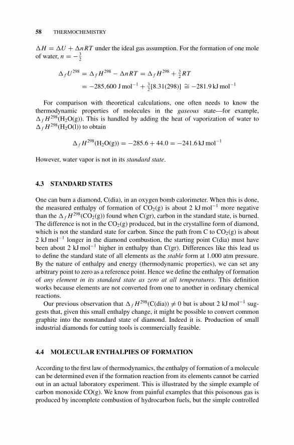
P1: OTA/XYZ P2: ABCc04 JWBS043-Rogers September 13, 2010 11:24 Printer Name: Yet to Come
58 THERMOCHEMISTRY
�H = �U + �n RT under the ideal gas assumption. For the formation of one moleof water, n = − 3
2
� f U 298 = � f H 298 − �n RT = � f H 298 + 32 RT
= −285,600 J mol−1 + 32 [8.31(298)] ∼= −281.9 kJ mol−1
For comparison with theoretical calculations, one often needs to know thethermodynamic properties of molecules in the gaseous state—for example,� f H 298(H2O(g)). This is handled by adding the heat of vaporization of water to� f H 298(H2O(l)) to obtain
� f H 298(H2O(g)) = −285.6 + 44.0 = −241.6 kJ mol−1
However, water vapor is not in its standard state.
4.3 STANDARD STATES
One can burn a diamond, C(dia), in an oxygen bomb calorimeter. When this is done,the measured enthalpy of formation of CO2(g) is about 2 kJ mol−1 more negativethan the � f H 298(CO2(g)) found when C(gr), carbon in the standard state, is burned.The difference is not in the CO2(g) produced, but in the crystalline form of diamond,which is not the standard state for carbon. Since the path from C to CO2(g) is about2 kJ mol−1 longer in the diamond combustion, the starting point C(dia) must havebeen about 2 kJ mol−1 higher in enthalpy than C(gr). Differences like this lead usto define the standard state of all elements as the stable form at 1.000 atm pressure.By the nature of enthalpy and energy (thermodynamic properties), we can set anyarbitrary point to zero as a reference point. Hence we define the enthalpy of formationof any element in its standard state as zero at all temperatures. This definitionworks because elements are not converted from one to another in ordinary chemicalreactions.
Our previous observation that � f H 298(C(dia)) �= 0 but is about 2 kJ mol−1 sug-gests that, given this small enthalpy change, it might be possible to convert commongraphite into the nonstandard state of diamond. Indeed it is. Production of smallindustrial diamonds for cutting tools is commercially feasible.
4.4 MOLECULAR ENTHALPIES OF FORMATION
According to the first law of thermodynamics, the enthalpy of formation of a moleculecan be determined even if the formation reaction from its elements cannot be carriedout in an actual laboratory experiment. This is illustrated by the simple example ofcarbon monoxide CO(g). We know from painful examples that this poisonous gas isproduced by incomplete combustion of hydrocarbon fuels, but the simple controlled
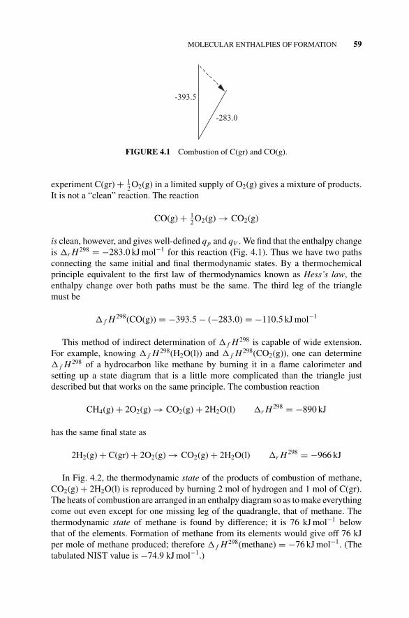
P1: OTA/XYZ P2: ABCc04 JWBS043-Rogers September 13, 2010 11:24 Printer Name: Yet to Come
MOLECULAR ENTHALPIES OF FORMATION 59
-393.5
-283.0
FIGURE 4.1 Combustion of C(gr) and CO(g).
experiment C(gr) + 12 O2(g) in a limited supply of O2(g) gives a mixture of products.
It is not a “clean” reaction. The reaction
CO(g) + 12 O2(g) → CO2(g)
is clean, however, and gives well-defined qp and qV . We find that the enthalpy changeis �r H 298 = −283.0 kJ mol−1 for this reaction (Fig. 4.1). Thus we have two pathsconnecting the same initial and final thermodynamic states. By a thermochemicalprinciple equivalent to the first law of thermodynamics known as Hess’s law, theenthalpy change over both paths must be the same. The third leg of the trianglemust be
� f H 298(CO(g)) = −393.5 − (−283.0) = −110.5 kJ mol−1
This method of indirect determination of � f H 298 is capable of wide extension.For example, knowing � f H 298(H2O(l)) and � f H 298(CO2(g)), one can determine� f H 298 of a hydrocarbon like methane by burning it in a flame calorimeter andsetting up a state diagram that is a little more complicated than the triangle justdescribed but that works on the same principle. The combustion reaction
CH4(g) + 2O2(g) → CO2(g) + 2H2O(l) �r H 298 = −890 kJ
has the same final state as
2H2(g) + C(gr) + 2O2(g) → CO2(g) + 2H2O(l) �r H 298 = −966 kJ
In Fig. 4.2, the thermodynamic state of the products of combustion of methane,CO2(g) + 2H2O(l) is reproduced by burning 2 mol of hydrogen and 1 mol of C(gr).The heats of combustion are arranged in an enthalpy diagram so as to make everythingcome out even except for one missing leg of the quadrangle, that of methane. Thethermodynamic state of methane is found by difference; it is 76 kJ mol−1 belowthat of the elements. Formation of methane from its elements would give off 76 kJper mole of methane produced; therefore � f H 298(methane) = −76 kJ mol−1. (Thetabulated NIST value is −74.9 kJ mol−1.)
P1: OTA/XYZ P2: ABCc04 JWBS043-Rogers September 13, 2010 11:24 Printer Name: Yet to Come
60 THERMOCHEMISTRY
2(286)=572
394
-890
-76
methane
elements
CO2 + 2H2O
FIGURE 4.2 A Thermochemical cycle for determining � f H 298(methane). Not to scale.
The indirect method shown for methane has been extended to very many hydro-carbons and other organic compounds. Although many inorganic substances do notburn, they do react. Inorganic reaction cycles similar to Fig. 4.2 can often be set upto obtain thermochemical data. A free thermochemical database is maintained bythe National Institutes of Standards and Technology (NIST) of the US government(.gov). Go to webbook.nist.gov.
4.5 ENTHALPIES OF REACTION
Suppose we know the enthalpies of formation � f H 298 of acetylene CH CH, etheneCH2 CH2, and ethane CH3CH3 (226.7, 52.5, and −84.7 kJ mol−1) by the combustionmethod shown in Fig. 4.1. The enthalpy change �r H 298 of the reaction
CH CH(g) + 2H2(g) → CH3CH3(g)
can be found by comparing the level given by � f H 298(CH CH(g)) with that of� f H 298(CH3CH3(g)). (Remember that � f H 298 is zero for elemental hydrogen.)
�r H 298 = � f H 298(CH3CH3(g)) − � f H 298(CH CH(g))
= −84.7 − 226.7 = −311.4 kJ mol−1
This reaction has been carried out with the result �r H 298 = −312.1 ± 0.6kJ mol−1.
A similar reaction, the partial hydrogenation,
CH CH(g) + H2(g) → CH2 CH2(g)
cannot be carried out in the laboratory. Hydrogenation doesn’t stop at CH2 CH2(g),but goes on to the fully hydrogenated product CH3CH3(g) or gives a mixed product
P1: OTA/XYZ P2: ABCc04 JWBS043-Rogers September 13, 2010 11:24 Printer Name: Yet to Come
ENTHALPIES OF REACTION 61
under all known experimental conditions. That doesn’t matter because of Hess’s law.The enthalpies of formation yield
�r H 298 = � f H 298(CH2 CH2(g)) − � f H 298(CH CH(g))
= 52.5 − 226.7 = −174.4 kJ mol−1
An equivalent way of finding �r H 298 of partial hydrogenation is by measuringthe enthalpy change −136.3 kJ mol−1 for the reaction
CH2 CH2(g) + H2 → CH3CH3(g)
When this is done, one has a first law triangle like that of Fig. 4.1, with only �r H 298
of partial hydrogenation yet to be determined. It is
�r H 298(partial) = −312.1 − (−136.3) = −175.8 kJ mol−1
as compared to the previous value of −174.4 kJ mol−1.One can also find the enthalpy of hydrogenation of ethene:
�r H 298 = � f H 298(CH3CH3(g)) − � f H 298(CH2 CH2(g))
= −84.7 − 52.5 = −137.2 kJ mol−1
This is a complete reaction to a well-defined final state. It has been carried out in thelaboratory. The experimental value is −136.3 ± 0.2 kJ mol−1.
Although, for simplicity, we shall use hydrocarbons to illustrate the principlesof thermochemistry, there is no such restriction in practice. For example, Pitzeret al. (1961) give the standard enthalpies of formation � f H ◦(KCl) = −435.9 and� f H ◦(KClO3) = −391.2 kJ mol−1. (The superscript ◦ indicates the standard state inthis notation; please do not confuse it with a superscripted zero of temperature 0.)These values lead to the enthalpy of reaction �r H ◦ necessary to convert solid KCl(s)to solid KClO3(s):
KCl(s) + 32 O2(g) → KClO3(s)
�r H ◦ = −391.2 − (−435.9) = 44.7 kJ mol−1
Including the notation (s) to indicate the solid state is a precaution rather than anecessity because in the standard states, both KCl and KClO3 are solids.
Even from these few simple examples, it should be clear that with a sufficientdatabase of enthalpies of formation, it is possible to calculate the enthalpies of analmost limitless array of chemical reactions of industrial, medical, and pharmaceuticalimportance. This is the reason why so much effort has gone into populating the
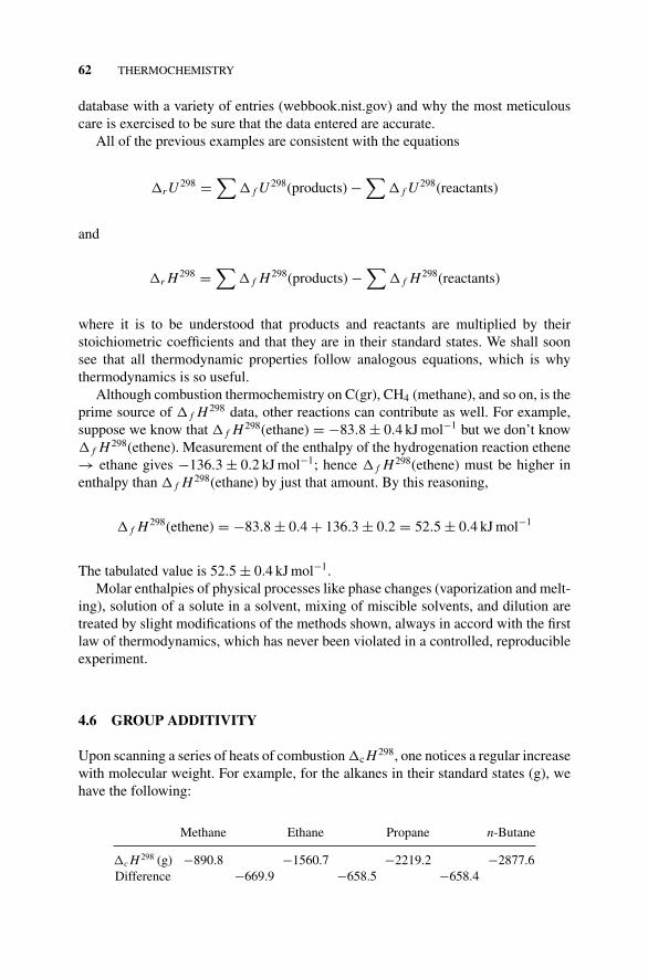
P1: OTA/XYZ P2: ABCc04 JWBS043-Rogers September 13, 2010 11:24 Printer Name: Yet to Come
62 THERMOCHEMISTRY
database with a variety of entries (webbook.nist.gov) and why the most meticulouscare is exercised to be sure that the data entered are accurate.
All of the previous examples are consistent with the equations
�rU 298 =∑
� f U 298(products) −∑
� f U 298(reactants)
and
�r H 298 =∑
� f H 298(products) −∑
� f H 298(reactants)
where it is to be understood that products and reactants are multiplied by theirstoichiometric coefficients and that they are in their standard states. We shall soonsee that all thermodynamic properties follow analogous equations, which is whythermodynamics is so useful.
Although combustion thermochemistry on C(gr), CH4 (methane), and so on, is theprime source of � f H 298 data, other reactions can contribute as well. For example,suppose we know that � f H 298(ethane) = −83.8 ± 0.4 kJ mol−1 but we don’t know� f H 298(ethene). Measurement of the enthalpy of the hydrogenation reaction ethene→ ethane gives −136.3 ± 0.2 kJ mol−1; hence � f H 298(ethene) must be higher inenthalpy than � f H 298(ethane) by just that amount. By this reasoning,
� f H 298(ethene) = −83.8 ± 0.4 + 136.3 ± 0.2 = 52.5 ± 0.4 kJ mol−1
The tabulated value is 52.5 ± 0.4 kJ mol−1.Molar enthalpies of physical processes like phase changes (vaporization and melt-
ing), solution of a solute in a solvent, mixing of miscible solvents, and dilution aretreated by slight modifications of the methods shown, always in accord with the firstlaw of thermodynamics, which has never been violated in a controlled, reproducibleexperiment.
4.6 GROUP ADDITIVITY
Upon scanning a series of heats of combustion �c H 298, one notices a regular increasewith molecular weight. For example, for the alkanes in their standard states (g), wehave the following:
Methane Ethane Propane n-Butane
�c H 298 (g) −890.8 −1560.7 −2219.2 −2877.6Difference −669.9 −658.5 −658.4
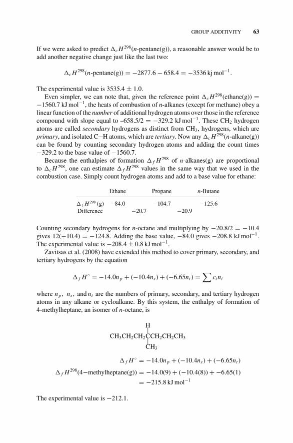
P1: OTA/XYZ P2: ABCc04 JWBS043-Rogers September 13, 2010 11:24 Printer Name: Yet to Come
GROUP ADDITIVITY 63
If we were asked to predict �c H 298(n-pentane(g)), a reasonable answer would be toadd another negative change just like the last two:
�c H 298(n-pentane(g)) = −2877.6 − 658.4 = −3536 kj mol−1.
The experimental value is 3535.4 ± 1.0.Even simpler, we can note that, given the reference point �c H 298(ethane(g)) =
−1560.7 kJ mol−1, the heats of combustion of n-alkanes (except for methane) obey alinear function of the number of additional hydrogen atoms over those in the referencecompound with slope equal to –658.5/2 = −329.2 kJ mol−1. These CH2 hydrogenatoms are called secondary hydrogens as distinct from CH3, hydrogens, which areprimary, and isolated C H atoms, which are tertiary. Now any �c H 298(n-alkane(g))can be found by counting secondary hydrogen atoms and adding the count times−329.2 to the base value of −1560.7.
Because the enthalpies of formation � f H 298 of n-alkanes(g) are proportionalto �c H 298, one can estimate � f H 298 values in the same way that we used in thecombustion case. Simply count hydrogen atoms and add to a base value for ethane:
Ethane Propane n-Butane
� f H 298 (g) −84.0 −104.7 −125.6Difference −20.7 −20.9
Counting secondary hydrogens for n-octane and multiplying by −20.8/2 = −10.4gives 12(−10.4) = −124.8. Adding the base value, −84.0 gives −208.8 kJ mol−1.The experimental value is −208.4 ± 0.8 kJ mol−1.
Zavitsas et al. (2008) have extended this method to cover primary, secondary, andtertiary hydrogens by the equation
� f H ◦ = −14.0n p + (−10.4ns) + (−6.65nt ) =∑
ci ni
where n p, ns, and nt are the numbers of primary, secondary, and tertiary hydrogenatoms in any alkane or cycloalkane. By this system, the enthalpy of formation of4-methylheptane, an isomer of n-octane, is
H|CH3CH2CH2CCH2CH2CH3|
CH3
� f H ◦ = −14.0n p + (−10.4ns) + (−6.65nt )
� f H 298(4−methylheptane(g)) = −14.0(9) + (−10.4(8)) + −6.65(1)
= −215.8 kJ mol−1
The experimental value is −212.1.
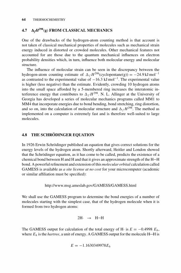
P1: OTA/XYZ P2: ABCc04 JWBS043-Rogers September 13, 2010 11:24 Printer Name: Yet to Come
64 THERMOCHEMISTRY
4.7 �fH298(g) FROM CLASSICAL MECHANICS
One of the drawbacks of the hydrogen-atom counting method is that account isnot taken of classical mechanical properties of molecules such as mechanical strainenergy induced in distorted or crowded molecules. Other mechanical features notaccounted for are those due to the quantum mechanical influences on electronprobability densities which, in turn, influence both molecular energy and molecularstructure.
The influence of molecular strain can be seen in the discrepancy between thehydrogen-atom counting estimate of � f H 298(cyclopentane(g)) = −24.9 kJ mol−1
as contrasted to the experimental value of −16.3 kJ mol−1. The experimental valueis higher (less negative) than the estimate. Evidently, crowding 10 hydrogen atomsinto the small space afforded by a 5-membered ring increases the interatomic in-terference energy that contributes to � f H 298. N. L. Allinger at the University ofGeorgia has developed a series of molecular mechanics programs called MM1 toMM4 that incorporate energies due to bond bending, bond stretching, ring distortion,and so on, into the calculation of molecular structure and � f H 298. The method asimplemented on a computer is extremely fast and is therefore well-suited to largemolecules.
4.8 THE SCHRODINGER EQUATION
In 1926 Erwin Schrodinger published an equation that gives correct solutions for theenergy levels of the hydrogen atom. Shortly afterward, Heitler and London showedthat the Schrodinger equation, as it has come to be called, predicts the existence of achemical bond between H and H and that it gives an approximate strength of the H Hbond. A powerful refinement and extension of this molecular orbital calculation calledGAMESS is available as a site license at no cost for your microcomputer (academicor similar affiliation must be specified):
http://www.msg.ameslab.gov/GAMESS/GAMESS.html
We shall use the GAMESS program to determine the bond energies of a number ofmolecules starting with the simplest case, that of the hydrogen molecule when it isformed from two hydrogen atoms:
2H· → H H
The GAMESS output for calculation of the total energy of H· is E = −0.4998 Eh ,where Eh is the hartree, a unit of energy. A GAMESS output for the molecule H H is
E = −1.1630349978Eh
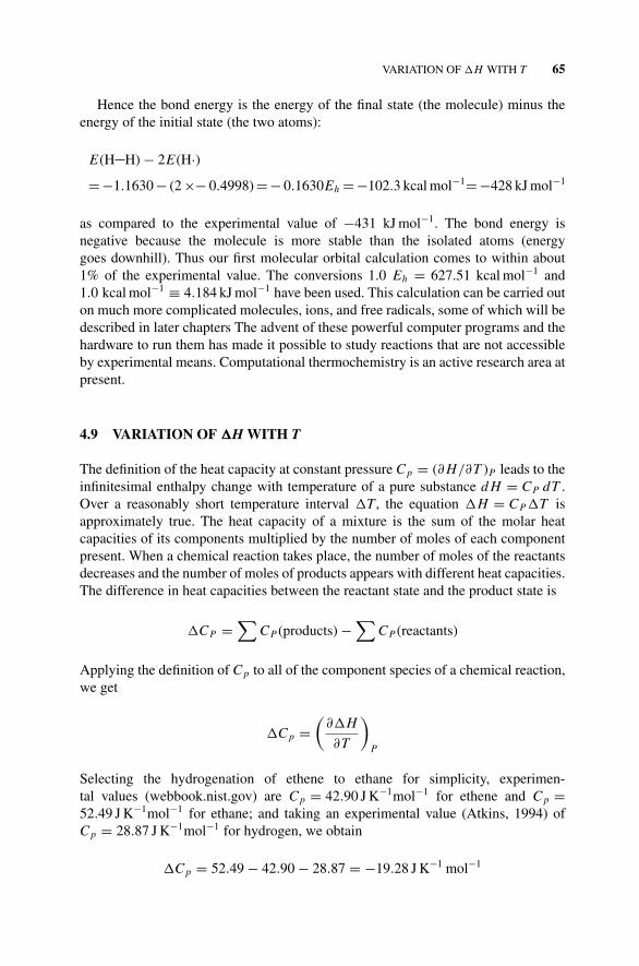
P1: OTA/XYZ P2: ABCc04 JWBS043-Rogers September 13, 2010 11:24 Printer Name: Yet to Come
VARIATION OF �H WITH T 65
Hence the bond energy is the energy of the final state (the molecule) minus theenergy of the initial state (the two atoms):
E(H H) − 2E(H·)= −1.1630 − (2 ×− 0.4998) = − 0.1630Eh = −102.3 kcal mol−1=−428 kJ mol−1
as compared to the experimental value of −431 kJ mol−1. The bond energy isnegative because the molecule is more stable than the isolated atoms (energygoes downhill). Thus our first molecular orbital calculation comes to within about1% of the experimental value. The conversions 1.0 Eh = 627.51 kcal mol−1 and1.0 kcal mol−1 ≡ 4.184 kJ mol−1 have been used. This calculation can be carried outon much more complicated molecules, ions, and free radicals, some of which will bedescribed in later chapters The advent of these powerful computer programs and thehardware to run them has made it possible to study reactions that are not accessibleby experimental means. Computational thermochemistry is an active research area atpresent.
4.9 VARIATION OF �H WITH T
The definition of the heat capacity at constant pressure C p = (∂ H/∂T )P leads to theinfinitesimal enthalpy change with temperature of a pure substance d H = CP dT .Over a reasonably short temperature interval �T , the equation �H = CP�T isapproximately true. The heat capacity of a mixture is the sum of the molar heatcapacities of its components multiplied by the number of moles of each componentpresent. When a chemical reaction takes place, the number of moles of the reactantsdecreases and the number of moles of products appears with different heat capacities.The difference in heat capacities between the reactant state and the product state is
�CP =∑
CP (products) −∑
CP (reactants)
Applying the definition of C p to all of the component species of a chemical reaction,we get
�C p =(
∂�H
∂T
)P
Selecting the hydrogenation of ethene to ethane for simplicity, experimen-tal values (webbook.nist.gov) are C p = 42.90 J K−1mol−1 for ethene and C p =52.49 J K−1mol−1 for ethane; and taking an experimental value (Atkins, 1994) ofC p = 28.87 J K−1mol−1 for hydrogen, we obtain
�C p = 52.49 − 42.90 − 28.87 = −19.28 J K−1 mol−1
P1: OTA/XYZ P2: ABCc04 JWBS043-Rogers September 13, 2010 11:24 Printer Name: Yet to Come
66 THERMOCHEMISTRY
The change in �r H for relatively small changes in T is �CP�T . We can test thisresult against experimental values for the simple hydrogenation of ethene (Kisti-akowsky et al., 1935). Using the computed result for �CP�T over the temperaturerange 355–298, the range between the temperature at which his experiments werecarried out (355 K) and standard temperature, we get
��hyd H 355 = −19.28 [− (355 − 298)] = 1.099 kJ mol−1
for the change in �hyd H 355, from 355 K, the temperature at which the hydrogenationwas actually carried out to room temperature 298 K. This small temperature correctiongives
�hyd H 298 = −137.44 + 1.10 = −136.34 kJ mol−1
for the enthalpy of hydrogenation of ethene at 298 K. This value is to be compared tothe result of a series of experiments carried out at 298 K by a different experimentalmethod which led to �hyd H 298 = −136.29 ± 0.21 kJ mol−1. The computed heatcapacities are probably reliable over a temperature range of ±50 K or so. Furthermore,the enthalpy of hydrogenation itself is insensitive to temperature, so we may takeexperimental determinations of �hyd H carried out under normal laboratory conditionsas essentially the same as the standard state �hyd H ◦
298.When calculations are carried out over larger temperature ranges, as they often are
in industrial applications, a polynomial approximation to the heat capacity is used.
C p = α + βT + γ T 2 + · · ·
This enables one to determine C p for the reactants and products of a chemical reactionat some new temperature other than 298 K, thereby enabling one to determine thenew change in heat capacity �C p for the reaction:
�CP =∑
CP (products) −∑
CP (reactants)
Variation in the�H of physical and chemical processes with variation in pressurecan be calculated from equations of state or by acquisition of experimental data andcurve fitting. Many reactions are less sensitive to pressure change than to temperaturechange over comparable ranges. Metiu (2006) has treated both temperature andpressure variation in the industrial production of ammonia from its elements.
4.10 DIFFERENTIAL SCANNING CALORIMETRY
When moderate amounts of heat are supplied to a solution of simple salts in water,we expect a smooth heating curve between, say 290 and 320 K, like the lower curvein Fig. 4.3. The heat capacity of water is nearly constant over this temperature range,

P1: OTA/XYZ P2: ABCc04 JWBS043-Rogers September 13, 2010 11:24 Printer Name: Yet to Come
DIFFERENTIAL SCANNING CALORIMETRY 67
and it will be little affected by small amounts of dissolved salts. Electrical circuitryexists that permits one to supply heat to a dilute solution in an adiabatic (insulated)calorimeter in very small pulses which may be regarded as infinitesimals dq. We nor-mally carry out the experiment at constant pressure, so the definition of heat capacityat constant pressure C p = dqp/dT is satisfied. The gradual temperature rise overmany small pulses can be followed by means of a thermistor circuit or its equivalent.
If, instead of a dilute solution of simple salts, the calorimeter contains a solutethat is capable of undergoing a thermal reaction, which is a reaction brought aboutby heat, the heating curve is more complicated. Thermal reactions are importantin many areas, especially in biochemistry. Proteins undergo heat denaturation. Heatdenaturation involves unfolding of the native protein and requires breaking of someor many of the bonds holding it in its native structure. Heat denaturation may bequite specific as to the temperature at which it occurs, and it may bring about subtlechanges in the protein, like changes in physiological activity, or it may bring aboutgross changes in the form of the protein as in the cooking of an egg.
Because heat denaturation involves breaking of internal bonds in the protein, itrequires an enthalpy input at constant pressure. The reaction is endoenthalpic. Adilute solution of salt and protein takes more heat to bring about a small temperaturechange than would the solution without the protein. The difference is observed onlyat or near the temperature of denaturation. Thus we have a normal temperature riseuntil denaturation begins, after which the heat capacity of the solution is abnormallylarge until we achieve complete thermal denaturation whereupon the temperature risedrops back to the normal baseline of a salt solution. Plotting C p as a function of T ,we see a peak at the denaturation temperature. This is the upper line in Fig. 4.3. Itis a simple matter to interface a computer to the scanning calorimeter output and tointegrate under the experimental curve:
�den H =∫ T f
Ti
C p dT
Cp
T
FIGURE 4.3 Schematic diagram of the thermal denaturation of a water-soluble protein. Thestraight line is the baseline of salt solution without protein. The peak is due to endoenthalpicdenaturation of the protein.
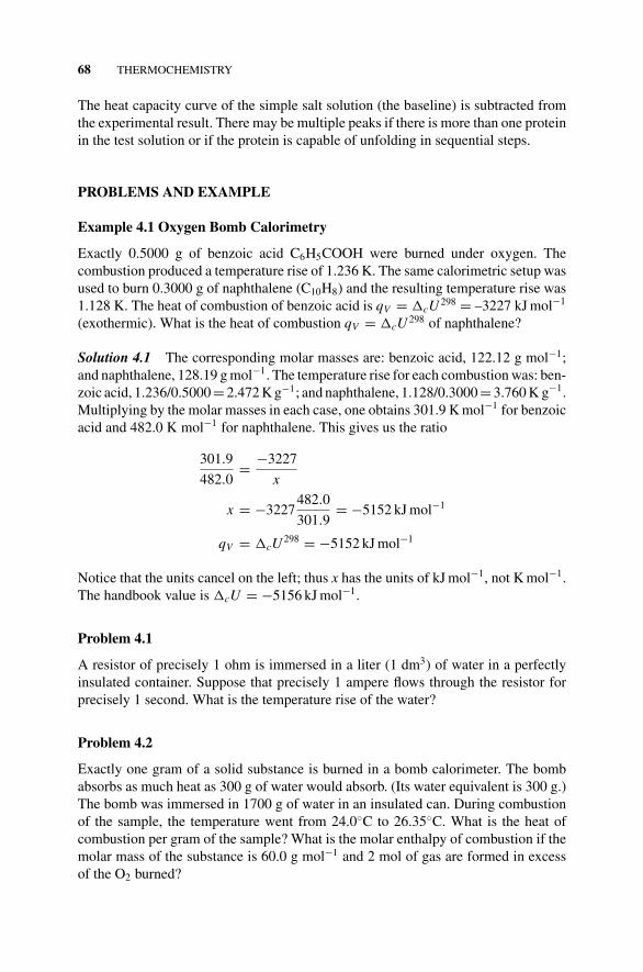
P1: OTA/XYZ P2: ABCc04 JWBS043-Rogers September 13, 2010 11:24 Printer Name: Yet to Come
68 THERMOCHEMISTRY
The heat capacity curve of the simple salt solution (the baseline) is subtracted fromthe experimental result. There may be multiple peaks if there is more than one proteinin the test solution or if the protein is capable of unfolding in sequential steps.
PROBLEMS AND EXAMPLE
Example 4.1 Oxygen Bomb Calorimetry
Exactly 0.5000 g of benzoic acid C6H5COOH were burned under oxygen. Thecombustion produced a temperature rise of 1.236 K. The same calorimetric setup wasused to burn 0.3000 g of naphthalene (C10H8) and the resulting temperature rise was1.128 K. The heat of combustion of benzoic acid is qV = �cU 298 = –3227 kJ mol−1
(exothermic). What is the heat of combustion qV = �cU 298 of naphthalene?
Solution 4.1 The corresponding molar masses are: benzoic acid, 122.12 g mol−1;and naphthalene, 128.19 g mol−1. The temperature rise for each combustion was: ben-zoic acid, 1.236/0.5000 = 2.472 K g−1; and naphthalene, 1.128/0.3000 = 3.760 K g−1.Multiplying by the molar masses in each case, one obtains 301.9 K mol−1 for benzoicacid and 482.0 K mol−1 for naphthalene. This gives us the ratio
301.9
482.0= −3227
x
x = −3227482.0
301.9= −5152 kJ mol−1
qV = �cU 298 = −5152 kJ mol−1
Notice that the units cancel on the left; thus x has the units of kJ mol−1, not K mol−1.The handbook value is �cU = −5156 kJ mol−1.
Problem 4.1
A resistor of precisely 1 ohm is immersed in a liter (1 dm3) of water in a perfectlyinsulated container. Suppose that precisely 1 ampere flows through the resistor forprecisely 1 second. What is the temperature rise of the water?
Problem 4.2
Exactly one gram of a solid substance is burned in a bomb calorimeter. The bombabsorbs as much heat as 300 g of water would absorb. (Its water equivalent is 300 g.)The bomb was immersed in 1700 g of water in an insulated can. During combustionof the sample, the temperature went from 24.0◦C to 26.35◦C. What is the heat ofcombustion per gram of the sample? What is the molar enthalpy of combustion if themolar mass of the substance is 60.0 g mol−1 and 2 mol of gas are formed in excessof the O2 burned?
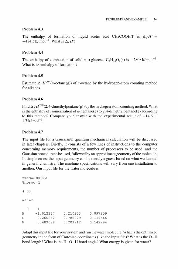
P1: OTA/XYZ P2: ABCc04 JWBS043-Rogers September 13, 2010 11:24 Printer Name: Yet to Come
PROBLEMS AND EXAMPLE 69
Problem 4.3
The enthalpy of formation of liquid acetic acid CH3COOH(l) is � f H ◦ =−484.5 kJ mol−1. What is �c H?
Problem 4.4
The enthalpy of combustion of solid α-d-glucose, C6H12O6(s) is −2808 kJ mol−1.What is its enthalpy of formation?
Problem 4.5
Estimate �c H 298(n-octane(g)) of n-octane by the hydrogen-atom counting methodfor alkanes.
Problem 4.6
Find � f H 298(2,4-dimethylpentane(g)) by the hydrogen atom counting method. Whatis the enthalpy of isomerization of n-heptane(g) to 2,4-dimethylpentane(g) accordingto this method? Compare your answer with the experimental result of −14.6 ±1.7 kJ mol−1.
Problem 4.7
The input file for a Gaussian C© quantum mechanical calculation will be discussedin later chapters. Briefly, it consists of a few lines of instructions to the computerconcerning memory requirements, the number of processors to be used, and theGaussian procedure to be used, followed by an approximate geometry of the molecule.In simple cases, the input geometry can be merely a guess based on what we learnedin general chemistry. The machine specifications will vary from one installation toanother. Our input file for the water molecule is
%mem=1800Mw%nproc=1
# g3
water
0 1H -1.012237 0.210253 0.097259O -0.260862 0.786229 0.119544H 0.489699 0.209212 0.142294
Adapt this input file for your system and run the water molecule. What is the optimizedgeometry in the form of Cartesian coordinates (like the input file)? What is the O Hbond length? What is the H O H bond angle? What energy is given for water?
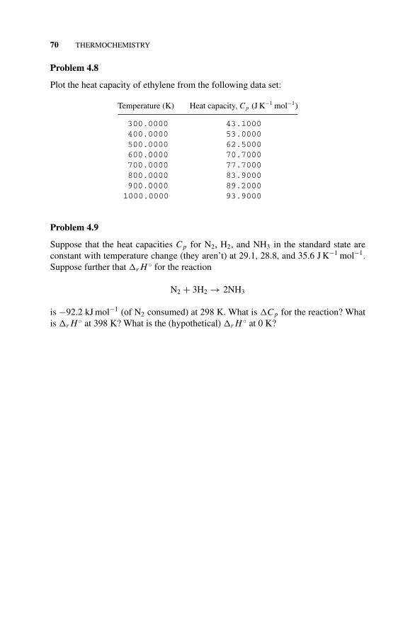
P1: OTA/XYZ P2: ABCc04 JWBS043-Rogers September 13, 2010 11:24 Printer Name: Yet to Come
70 THERMOCHEMISTRY
Problem 4.8
Plot the heat capacity of ethylene from the following data set:
Temperature (K) Heat capacity, Cp (J K−1 mol−1)
300.0000 43.1000400.0000 53.0000500.0000 62.5000600.0000 70.7000700.0000 77.7000800.0000 83.9000900.0000 89.20001000.0000 93.9000
Problem 4.9
Suppose that the heat capacities C p for N2, H2, and NH3 in the standard state areconstant with temperature change (they aren’t) at 29.1, 28.8, and 35.6 J K−1 mol−1.Suppose further that �r H ◦ for the reaction
N2 + 3H2 → 2NH3
is −92.2 kJ mol−1 (of N2 consumed) at 298 K. What is �C p for the reaction? Whatis �r H ◦ at 398 K? What is the (hypothetical) �r H ◦ at 0 K?
P1: OTA/XYZ P2: ABCc05 JWBS043-Rogers September 13, 2010 11:25 Printer Name: Yet to Come
5ENTROPY AND THE SECOND LAW
The second law of thermodynamics and the concept of entropy are firmly based onSadi Carnot’s somewhat abstract demonstration that the work done by drawing heatfrom a hot reservoir and expelling it to a cold reservoir is independent of the nature ofthe engine that carries out the work (Fig. 5.1). An especially readable description ofthe progression of Carnot’s abstract reflections on the efficiency of steam engines tothe form of the entropy function we use today was given by Kondipudi and Prigogine(1998). We shall not follow the historical development of this idea, interesting thoughit is; rather we shall jump right to Clausius’s definition of the entropy, LudwigBoltzmann’s statistical interpretation, and the influence of the second law on physicalphenomena and chemical reactions.
5.1 ENTROPY
In 1865, Rudolf Clausius showed that the cyclic integral∮
dq/T is zero for an
abstract Carnot engine operating reversibly around a cyclic path:
∮dq
T= 0
Thus the integrand, which Clausius named entropy and gave the symbol dS, isa thermodynamic function. This definition is one statement of the second law of
Concise Physical Chemistry, by Donald W. RogersCopyright C© 2011 John Wiley & Sons, Inc.
71
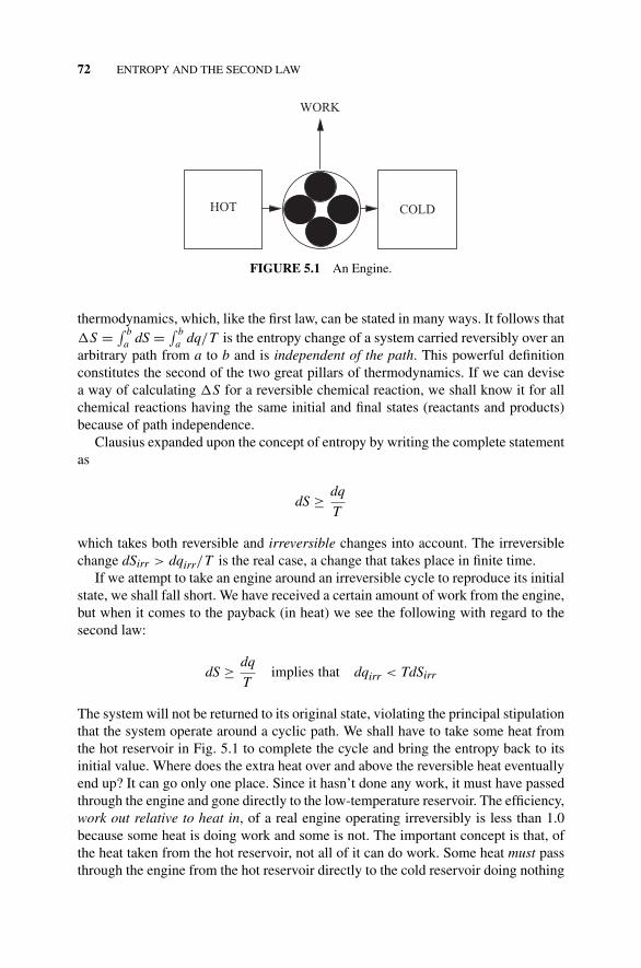
P1: OTA/XYZ P2: ABCc05 JWBS043-Rogers September 13, 2010 11:25 Printer Name: Yet to Come
72 ENTROPY AND THE SECOND LAW
HOT COLD
WORK
FIGURE 5.1 An Engine.
thermodynamics, which, like the first law, can be stated in many ways. It follows that�S = ∫ b
a dS = ∫ ba dq/T is the entropy change of a system carried reversibly over an
arbitrary path from a to b and is independent of the path. This powerful definitionconstitutes the second of the two great pillars of thermodynamics. If we can devisea way of calculating �S for a reversible chemical reaction, we shall know it for allchemical reactions having the same initial and final states (reactants and products)because of path independence.
Clausius expanded upon the concept of entropy by writing the complete statementas
dS ≥ dq
T
which takes both reversible and irreversible changes into account. The irreversiblechange dSirr > dqirr/T is the real case, a change that takes place in finite time.
If we attempt to take an engine around an irreversible cycle to reproduce its initialstate, we shall fall short. We have received a certain amount of work from the engine,but when it comes to the payback (in heat) we see the following with regard to thesecond law:
dS ≥ dq
Timplies that dqirr < TdSirr
The system will not be returned to its original state, violating the principal stipulationthat the system operate around a cyclic path. We shall have to take some heat fromthe hot reservoir in Fig. 5.1 to complete the cycle and bring the entropy back to itsinitial value. Where does the extra heat over and above the reversible heat eventuallyend up? It can go only one place. Since it hasn’t done any work, it must have passedthrough the engine and gone directly to the low-temperature reservoir. The efficiency,work out relative to heat in, of a real engine operating irreversibly is less than 1.0because some heat is doing work and some is not. The important concept is that, ofthe heat taken from the hot reservoir, not all of it can do work. Some heat must passthrough the engine from the hot reservoir directly to the cold reservoir doing nothing

P1: OTA/XYZ P2: ABCc05 JWBS043-Rogers September 13, 2010 11:25 Printer Name: Yet to Come
ENTROPY 73
but restoring the system entropy to its original state. Because of this necessity, someof the heat drawn from the hot reservoir in an irreversible cycle is unavailable to dowork.
5.1.1 Heat Death and Time’s Arrow
Because there is always heat transferred to the surroundings in an irreversible cycle,the entropy of the system plus the surroundings always increases. If we take theuniverse as the surroundings, then since all real processes are irreversible we havea consequence of the second law: The entropy of the universe tends to a maximum.When the universe has reached its maximum entropy, no more irreversible changewill be possible. The driving force of change will be gone. This is called the heatdeath of the universe. In case you are worried, it is calculated to be in the far distantfuture.
The entropy of the universe must be greater after an irreversible change hasoccurred than it was before the change, so we have a thermodynamic definition ofthe direction of time (which the first law doesn’t give). Time must go from beforethe change to after the change; it cannot go in the reverse direction.1 Entropy issometimes called “time’s arrow.”
5.1.2 The Reaction Coordinate
Prigogine has defined a reaction coordinate ξ which progresses as a chemical reactiontakes place. Starting with pure reactant A, the reaction coordinate increases as productB is produced:
A → B
At some point, the time derivative of ξ becomes zero and the reaction stops insofar asmacroscopic concentration measurements are concerned.2 When the time derivativeof the reaction coordinate is zero, the system consisting of nA + nB is at equilibrium.Because there are no macroscopic concentration changes, the ratio of the mole num-bers of reactant and product nB/n A is constant. It is called the equilibrium constantKeq:
(∂ξ
∂t
)T,p
= 0
Keq = nB/nA
It would be appealing to think that the reaction coordinate is determined solely bythe energy U or enthalpy H of the system flowing from a high level to a low level,
1Classical thermodynamics does not include QED.2There are microscopic exchanges between species A and B, but they are equal and opposite on averageso they do not bring about measurable concentration changes.
P1: OTA/XYZ P2: ABCc05 JWBS043-Rogers September 13, 2010 11:25 Printer Name: Yet to Come
74 ENTROPY AND THE SECOND LAW
but this is not the case. There is more to think about in a chemical or physical changethan just minimization of U or H. There is the question of order and disorder of thereactant state and the product state.
5.1.3 Disorder
When we look at a chemical reaction
A → B
or an analogous physical change
A(l) → A(g)
we must look at the driving force that produces the change. Part of that force comesfrom the tendency to seek a minimum (water flows downhill), but part of it comesfrom the universal tendency of thermodynamic systems to seek maximum disorder.A familiar example is vaporization of a liquid such as water.
The liquid state, though not perfectly ordered, is held together by strong inter-molecular forces. These are the very forces that we say are nonexistent or negligiblein the vapor state. The entropy change for many liquids is about 88 J K−1 mol−1, arule known as Trouton’s rule, that has been verified many times over for liquids asdiverse as liquid Cl2, HCl, chloroform, and the n-alkanes. Liquids that deviate fromthis rule do so, not because of any failure of the entropy concept for vaporization, butbecause of abnormal forces in the liquid state. An example is water, which deviatesa little due to hydrogen bonding, and hydrogen fluoride HF, which deviates a lot.
5.2 ENTROPY CHANGES
In general, the entropy change for any change of state, including melting and change incrystalline form in the solid state, is given by the enthalpy change and the temperatureappropriate to the change or transition considered:
�S = �Htrans
Ttrans
5.2.1 Heating
The entropy of heating of an ideal gas is positive because thermal agitation makesthe high-temperature state more disordered than the low-temperature state. From theexpression for molar heat capacity, one has
C p =(
∂ H
∂T
)p
P1: OTA/XYZ P2: ABCc05 JWBS043-Rogers September 13, 2010 11:25 Printer Name: Yet to Come
ENTROPY CHANGES 75
Hence
dSrev ≡ dqrev
T= dH
T= C p
dT
T
Taking the integrals over the interval T1 to T2, we obtain
�S =∫ T2
T1
C pdT
T= C p
∫ T2
T1
dT
T= C p ln
T2
T1
for the molar entropy change of heating at constant pressure. There is an analogousequation for the energy change of heating at constant volume.
5.2.2 Expansion
For expansion at constant temperature, U is constant. The first law dU = dq + dw = 0gives us dq = dw and the second law gives us
dSrev = dqrev
T= dw
T= pdV
T
for reversible pressure–volume work. Taking the gas to be ideal for simplicity, weobtain
dSrev = p dV
T=
RTV dV
T= R
dV
V
Integrating between limits as before, we obtain
�Srev = R∫ V2
V1
dV
V= R ln
V2
V1
for the reversible expansion of one mole of an ideal gas from V1 to V2. The right-handside of the equation should be multiplied by n for expansion of n moles of gas. If thegas is not ideal, a real gas equation can be substituted for the ideal gas law in theseequations. Thus, the mathematical complexity will be increased, but the principle isthe same.
5.2.3 Heating and Expansion
Because dS is an exact differential and S = f (T, p), we have
dS =(
∂S
∂T
)p
dT +(
∂S
∂p
)T
dp
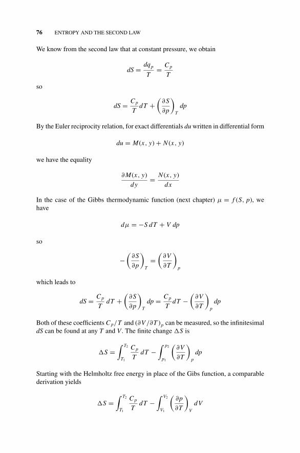
P1: OTA/XYZ P2: ABCc05 JWBS043-Rogers September 13, 2010 11:25 Printer Name: Yet to Come
76 ENTROPY AND THE SECOND LAW
We know from the second law that at constant pressure, we obtain
dS = dqp
T= C p
T
so
dS = C p
TdT +
(∂S
∂p
)T
dp
By the Euler reciprocity relation, for exact differentials du written in differential form
du = M(x, y) + N (x, y)
we have the equality
∂ M(x, y)
dy= N (x, y)
dx
In the case of the Gibbs thermodynamic function (next chapter) µ = f (S, p), wehave
dµ = −S dT + V dp
so
−(
∂S
∂p
)T
=(
∂V
∂T
)p
which leads to
dS = C p
TdT +
(∂S
∂p
)T
dp = C p
TdT −
(∂V
∂T
)p
dp
Both of these coefficients C p/T and (∂V /∂T )p can be measured, so the infinitesimaldS can be found at any T and V . The finite change �S is
�S =∫ T2
T1
C p
TdT −
∫ p2
p1
(∂V
∂T
)p
dp
Starting with the Helmholtz free energy in place of the Gibs function, a comparablederivation yields
�S =∫ T2
T1
C p
TdT −
∫ V2
V1
(∂p
∂T
)V
dV
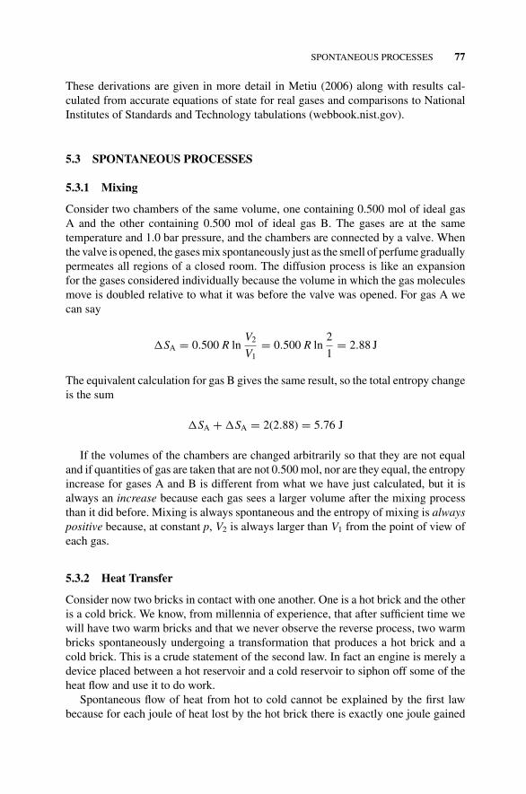
P1: OTA/XYZ P2: ABCc05 JWBS043-Rogers September 13, 2010 11:25 Printer Name: Yet to Come
SPONTANEOUS PROCESSES 77
These derivations are given in more detail in Metiu (2006) along with results cal-culated from accurate equations of state for real gases and comparisons to NationalInstitutes of Standards and Technology tabulations (webbook.nist.gov).
5.3 SPONTANEOUS PROCESSES
5.3.1 Mixing
Consider two chambers of the same volume, one containing 0.500 mol of ideal gasA and the other containing 0.500 mol of ideal gas B. The gases are at the sametemperature and 1.0 bar pressure, and the chambers are connected by a valve. Whenthe valve is opened, the gases mix spontaneously just as the smell of perfume graduallypermeates all regions of a closed room. The diffusion process is like an expansionfor the gases considered individually because the volume in which the gas moleculesmove is doubled relative to what it was before the valve was opened. For gas A wecan say
�SA = 0.500 R lnV2
V1= 0.500 R ln
2
1= 2.88 J
The equivalent calculation for gas B gives the same result, so the total entropy changeis the sum
�SA + �SA = 2(2.88) = 5.76 J
If the volumes of the chambers are changed arbitrarily so that they are not equaland if quantities of gas are taken that are not 0.500 mol, nor are they equal, the entropyincrease for gases A and B is different from what we have just calculated, but it isalways an increase because each gas sees a larger volume after the mixing processthan it did before. Mixing is always spontaneous and the entropy of mixing is alwayspositive because, at constant p, V2 is always larger than V1 from the point of view ofeach gas.
5.3.2 Heat Transfer
Consider now two bricks in contact with one another. One is a hot brick and the otheris a cold brick. We know, from millennia of experience, that after sufficient time wewill have two warm bricks and that we never observe the reverse process, two warmbricks spontaneously undergoing a transformation that produces a hot brick and acold brick. This is a crude statement of the second law. In fact an engine is merely adevice placed between a hot reservoir and a cold reservoir to siphon off some of theheat flow and use it to do work.
Spontaneous flow of heat from hot to cold cannot be explained by the first lawbecause for each joule of heat lost by the hot brick there is exactly one joule gained
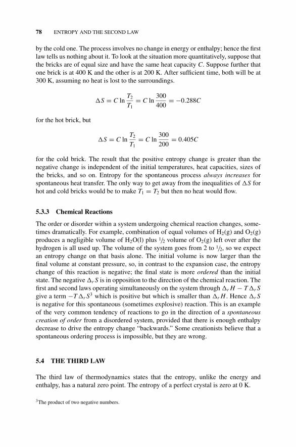
P1: OTA/XYZ P2: ABCc05 JWBS043-Rogers September 13, 2010 11:25 Printer Name: Yet to Come
78 ENTROPY AND THE SECOND LAW
by the cold one. The process involves no change in energy or enthalpy; hence the firstlaw tells us nothing about it. To look at the situation more quantitatively, suppose thatthe bricks are of equal size and have the same heat capacity C. Suppose further thatone brick is at 400 K and the other is at 200 K. After sufficient time, both will be at300 K, assuming no heat is lost to the surroundings.
�S = C lnT2
T1= C ln
300
400= −0.288C
for the hot brick, but
�S = C lnT2
T1= C ln
300
200= 0.405C
for the cold brick. The result that the positive entropy change is greater than thenegative change is independent of the initial temperatures, heat capacities, sizes ofthe bricks, and so on. Entropy for the spontaneous process always increases forspontaneous heat transfer. The only way to get away from the inequalities of �S forhot and cold bricks would be to make T1 = T2 but then no heat would flow.
5.3.3 Chemical Reactions
The order or disorder within a system undergoing chemical reaction changes, some-times dramatically. For example, combination of equal volumes of H2(g) and O2(g)produces a negligible volume of H2O(l) plus 1/2 volume of O2(g) left over after thehydrogen is all used up. The volume of the system goes from 2 to 1/2, so we expectan entropy change on that basis alone. The initial volume is now larger than thefinal volume at constant pressure, so, in contrast to the expansion case, the entropychange of this reaction is negative; the final state is more ordered than the initialstate. The negative �r S is in opposition to the direction of the chemical reaction. Thefirst and second laws operating simultaneously on the system through �r H − T �r Sgive a term −T �r S3 which is positive but which is smaller than �r H . Hence �r Sis negative for this spontaneous (sometimes explosive) reaction. This is an exampleof the very common tendency of reactions to go in the direction of a spontaneouscreation of order from a disordered system, provided that there is enough enthalpydecrease to drive the entropy change “backwards.” Some creationists believe that aspontaneous ordering process is impossible, but they are wrong.
5.4 THE THIRD LAW
The third law of thermodynamics states that the entropy, unlike the energy andenthalpy, has a natural zero point. The entropy of a perfect crystal is zero at 0 K.
3The product of two negative numbers.
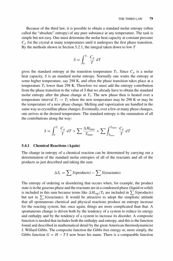
P1: OTA/XYZ P2: ABCc05 JWBS043-Rogers September 13, 2010 11:25 Printer Name: Yet to Come
THE THIRD LAW 79
Because of the third law, it is possible to obtain a standard molar entropy (oftencalled the “absolute” entropy) of any pure substance at any temperature. The task issimple but not easy. One must determine the molar heat capacity at constant pressureC p for the crystal at many temperatures until it undergoes the first phase transition.By the methods shown in Section 5.2.1, the integral taken down to low T
S =∫ T1
0
C p
TdT
gives the standard entropy at the transition temperature T1. Since C p is a molarheat capacity, S is an standard molar entropy. Normally one wants the entropy atsome higher temperature, say 298 K, and often the phase transition takes place at atemperature T1 lower than 298 K. Therefore we must add the entropy contributionfrom the phase transition to the value of S that we already have to obtain the standardmolar entropy after the phase change at T1. The new phase then is heated over atemperature interval T1 → T2 where the new temperature may be 298 K or may bethe temperature of a new phase change. Melting and vaporization are handled in thesame way as crystalline phase changes. Eventually, over a few or many phase changes,one arrives at the desired temperature. The standard entropy is the summation of allthe contributions along the way:
S =∫ T1
0
C p
TdT +
∑ �Htrans
Ttrans+
∑ ∫ Thigher
Tlower
C p
TdT
5.4.1 Chemical Reactions (Again)
The change in entropy of a chemical reaction can be determined by carrying out adetermination of the standard molar entropies of all of the reactants and all of theproducts as just described and taking the sum
�Sr =∑
S(products) −∑
S(reactants)
The entropy of ordering or disordering that occurs when, for example, the productstate is in the gaseous phase and the reactants are in a condensed phase (liquid or solid)is included in this sum because terms like �Hvap/Tb are included in
∑S(products)
but not in∑
S(reactants). It would be attractive to adopt the simplistic attitudethat all spontaneous chemical and physical reactions produce an entropy increasefor the reacting system, but, once again, things are more complicated than that. Aspontaneous change is driven both by the tendency of a system to reduce its energyand enthalpy and by the tendency of a system to increase its disorder. A compositefunction is needed that includes both the enthalpy and entropy, and this is the functionfound and described in mathematical detail by the great American thermodynamicistJ. Willard Gibbs. The composite function the Gibbs free energy or, more simply, theGibbs function G = H − T S now bears his name. There is a comparable function
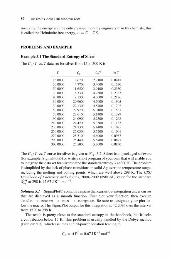
P1: OTA/XYZ P2: ABCc05 JWBS043-Rogers September 13, 2010 11:25 Printer Name: Yet to Come
80 ENTROPY AND THE SECOND LAW
involving the energy and the entropy used more by engineers than by chemists; thisis called the Helmholtz free energy, A = E − T S.
PROBLEMS AND EXAMPLE
Example 5.1 The Standard Entropy of Silver
The C p/T vs. T data set for silver from 15 to 300 K is
T Cp Cp/T ln T
15.0000 0.6700 2.7100 0.044730.0000 4.7700 3.4000 0.159050.0000 11.6500 3.9100 0.233070.0000 16.3300 4.2500 0.233390.0000 19.1300 4.5000 0.2126
110.0000 20.9600 4.7000 0.1905130.0000 22.1300 4.8700 0.1702150.0000 22.9700 5.0100 0.1531170.0000 23.6100 5.1400 0.1389190.0000 24.0900 5.2500 0.1268210.0000 24.4200 5.3500 0.1163230.0000 24.7300 5.4400 0.1075250.0000 25.0300 5.5200 0.1001270.0000 25.3100 5.6000 0.0937290.0000 25.4400 5.6700 0.0877300.0000 25.5000 5.7000 0.0850
The C p/T vs. T curve for silver is given as Fig. 5.2. Select from packaged software(for example, SigmaPlot C©) or write a short program of your own that will enable youto integrate the data set for silver to find the standard entropy S at 300 K. The problemis simplified by the lack of phase transitions in solid Ag over the temperature range,including the melting and boiling points, which are well above 298 K. The CRCHandbook of Chemistry and Physics, 2008–2009 (89th ed.) value for the standardS298
Ag at 298 is 42.67 J K−1 mol−1.
Solution 5.1 SigmaPlot C© contains a macro that carries out integration under curvesthat are displayed as a smooth function. First plot your function, then executeTools → macro → run → compute. Be sure to designate your plot be-low the macro. The SigmaPlot output for this integration is 42.2076 over the intervalfrom 15 K to 298 K.
The result is pretty close to the standard entropy in the handbook, but it lacksa contribution below 15 K. This problem is usually handled by the Debye method(Problem 5.7), which assumes a third-power equation leading to
C p = AT 3 = 0.67 J K−1 mol−1
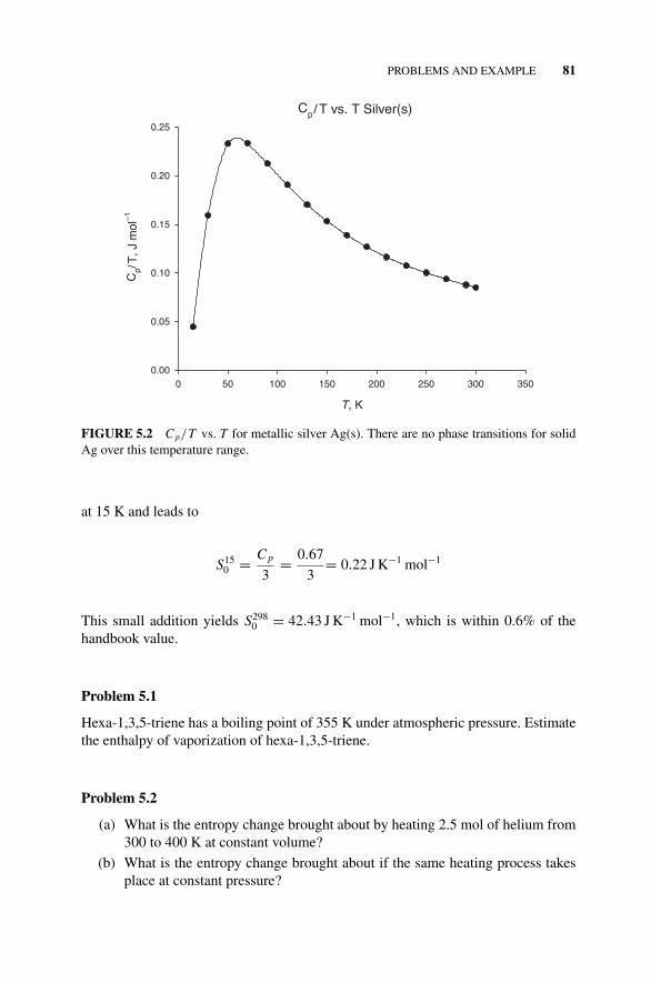
P1: OTA/XYZ P2: ABCc05 JWBS043-Rogers September 13, 2010 11:25 Printer Name: Yet to Come
PROBLEMS AND EXAMPLE 81
Cp/ T vs. T Silver(s)
T, K
0 50 100 150 200 250 300 350
Cp/
T, J
mol
–1
0.00
0.05
0.10
0.15
0.20
0.25
FIGURE 5.2 Cp/T vs. T for metallic silver Ag(s). There are no phase transitions for solidAg over this temperature range.
at 15 K and leads to
S150 = C p
3= 0.67
3= 0.22 J K−1 mol−1
This small addition yields S2980 = 42.43 J K−1 mol−1, which is within 0.6% of the
handbook value.
Problem 5.1
Hexa-1,3,5-triene has a boiling point of 355 K under atmospheric pressure. Estimatethe enthalpy of vaporization of hexa-1,3,5-triene.
Problem 5.2
(a) What is the entropy change brought about by heating 2.5 mol of helium from300 to 400 K at constant volume?
(b) What is the entropy change brought about if the same heating process takesplace at constant pressure?
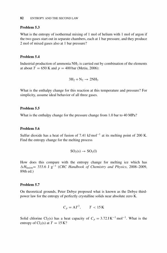
P1: OTA/XYZ P2: ABCc05 JWBS043-Rogers September 13, 2010 11:25 Printer Name: Yet to Come
82 ENTROPY AND THE SECOND LAW
Problem 5.3
What is the entropy of isothermal mixing of 1 mol of helium with 1 mol of argon ifthe two gases start out in separate chambers, each at 1 bar pressure, and they produce2 mol of mixed gases also at 1 bar pressure?
Problem 5.4
Industrial production of ammonia NH3 is carried out by combination of the elementsat about T = 650 K and p = 400 bar (Metiu, 2006):
3H2 + N2 → 2NH3
What is the enthalpy change for this reaction at this temperature and pressure? Forsimplicity, assume ideal behavior of all three gases.
Problem 5.5
What is the enthalpy change for the pressure change from 1.0 bar to 40 MPa?
Problem 5.6
Sulfur dioxide has a heat of fusion of 7.41 kJ mol−1 at its melting point of 200 K.Find the entropy change for the melting process
SO2(s) → SO2(l)
How does this compare with the entropy change for melting ice which has�Hfusion= 333.6 J g−1 (CRC Handbook of Chemistry and Physics, 2008–2009,89th ed.)
Problem 5.7
On theoretical grounds, Peter Debye proposed what is known as the Debye third-power law for the entropy of perfectly crystalline solids near absolute zero K.
C p = AT 3, T < 15 K
Solid chlorine Cl2(s) has a heat capacity of C p = 3.72 J K−1 mol−1. What is theentropy of Cl2(s) at T = 15 K?
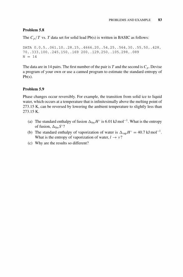
P1: OTA/XYZ P2: ABCc05 JWBS043-Rogers September 13, 2010 11:25 Printer Name: Yet to Come
PROBLEMS AND EXAMPLE 83
Problem 5.8
The C p/T vs. T data set for solid lead Pb(s) is written in BASIC as follows:
DATA 0,0,5,.061,10,.28,15,.4666,20,.54,25,.564,30,.55,50,.428,70,.333,100,.245,150,.169 200,.129,250,.105,298,.089N = 14
The data are in 14 pairs. The first number of the pair is T and the second is C p. Devisea program of your own or use a canned program to estimate the standard entropy ofPb(s).
Problem 5.9
Phase changes occur reversibly. For example, the transition from solid ice to liquidwater, which occurs at a temperature that is infinitesimally above the melting point of273.15 K, can be reversed by lowering the ambient temperature to slightly less than273.15 K.
(a) The standard enthalpy of fusion �fus H ◦ is 6.01 kJ mol−1. What is the entropyof fusion, �fusS◦?
(b) The standard enthalpy of vaporization of water is �vap H ◦ = 40.7 kJ mol−1.What is the entropy of vaporization of water, l → v?
(c) Why are the results so different?
P1: OTA/XYZ P2: ABCc06 JWBS043-Rogers September 13, 2010 11:25 Printer Name: Yet to Come
6THE GIBBS FREE ENERGY
Our brief consideration of engines and heat transfer showed that only part of the heattransferred from a hot reservoir to a cold one by a real process is available to dowork. This is the available or “free” energy that we have been seeking. In the theoryof steam engines, the Helmholtz free energy A = U − TS is central. In chemicalreactions the closely analogous Gibbs free energy G = H − TS is central. We shallbe mainly concerned with the Gibbs free energy.
6.1 COMBINING ENTHALPY AND ENTROPY
We seek a combined function that expresses the spontaneous tendency of a chemicalsystem to undergo a change in enthalpy simultaneously with a change in its entropy.In other words, we seek a factor that governs chemical reactions. Clearly, the signsof enthalpy and entropy must be opposite because one function tends to a maximumand the other tends to a minimum. We might write X = U − S for our unknownenergy function such that matter flows from a point of high potential to one of lowpotential in the way that water flows downhill, but we chemists are usually interestedin reactions that are carried out at constant pressure, so we substitute H for U in theequation. Also we notice that the units are wrong. Enthalpy has the unit J and entropyhas the unit J K−1. To bring everything into consistent units of energy, we multiplythe entropy by T to get the central equation of chemical thermodynamics:
G ≡ H − TS
Concise Physical Chemistry, by Donald W. RogersCopyright C© 2011 John Wiley & Sons, Inc.
84
P1: OTA/XYZ P2: ABCc06 JWBS043-Rogers September 13, 2010 11:25 Printer Name: Yet to Come
FREE ENERGIES OF FORMATION 85
This equation implies constant p by the use of H and constant T at thermal equilibrium.Multiplication of S by T is also consistent with the definition of entropy as d S =dq/T , where q is a reversible thermal energy or enthalpy. The infinitesimal and smallfinite expressions dG and �G are also implied:
dG = dH − T dS
and
�G = �H − T �S
The Gibbs function is the algebraic sum of a thermodynamic state function H anda constant times a thermodynamic function –TS, hence it is a thermodynamic statefunction as well.
The terms Gibbs state function, Gibbs free energy, and chemical potential are allused for the thermodynamic property G. Usually the first term is used to stress themathematical properties of the function, the second is used in general descriptions,and the third is used to stress the intensive nature of the molar free energy µ = G/n.We shall use these terms more or less synonymously, relying on context to make themeaning clear or reminding the reader, from time to time, of the distinction betweenthe molar Gibbs free energy G and the extensive Gibbs function G. The term chemicalpotential, for the molar (or partial molar) quantity µ, depicts well the property ofchemical systems to flow down a gradient toward a minimum that we refer to as anequilibrium point.
6.2 FREE ENERGIES OF FORMATION
At this point, we are able to determine the enthalpy change of a chemical reaction bydirect or indirect calorimetric measurement of � f H of the participants in the reactionand we can find the corresponding entropy change by integration of heat capacity datafor each of the participants. These results permit us to calculate Gibbs free energiesof formation. Suppose that we select combustion of C(graphite) in O2(g) to formCO2(g) as the illustrative case and that we have determined the standard entropiesof these three species to be 5.74, 205.138, and 213.74 J K−1 mol−1, respectively. Weapply the general formula
�S298r =
∑S(products) −
∑S(reactants)
to the reaction
C(gr) + O2(g) → CO2(g)
P1: OTA/XYZ P2: ABCc06 JWBS043-Rogers September 13, 2010 11:25 Printer Name: Yet to Come
86 THE GIBBS FREE ENERGY
to get
�S298r = 213.74 − 5.74 − 205.138 = 2.862 J K−1mol−1
as the change in standard entropy of the reacting system.The enthalpy of formation of CO2(g) has been measured and found to be −393.51
kJ mol−1 (Section 4.2), so from the fundamental equation for a finite change (�G)
�G = �H − T �S
we get
�G f = �H f − T �S f = −393.51 − 298(2.862 × 10⁻³)
= −393.51 − 0.852 = −394.36 kJ mol−1
which is the Gibbs function of formation at 298 K of CO2(g).Comparable calculations yield the Gibbs functions of many direct formation reac-
tions of elements to their compounds. Armed with these Gibbs functions of formation,we can manipulate them to find the Gibbs functions of compounds not cleanly formedfrom their elements in the same way as we did for the enthalpies of formation.
6.3 SOME FUNDAMENTAL THERMODYNAMIC IDENTITIES
For a reversible change doing only pV work, the first law gives
dU = dq − dw = TdS − p dV
whence, knowing that U = f (S,V ), dU = (∂U/∂S)V dS + (∂U/∂V )S dV, we findthat
(∂U
∂S
)V
= T and
(∂U
∂V
)S
= −p
Also, G = f (p,T ), dG =(
∂G
∂p
)T
dp +(
∂G
∂T
)p
dT , and
dG = V dp − S dT
with the results that
(∂G
∂p
)T
= V and
(∂G
∂T
)p
= −S
P1: OTA/XYZ P2: ABCc06 JWBS043-Rogers September 13, 2010 11:25 Printer Name: Yet to Come
PRESSURE DEPENDENCE OF THE CHEMICAL POTENTIAL 87
6.4 THE FREE ENERGY OF REACTION
We have procedures that give us the enthalpies of formation of the participants inany reaction at 1.0 atm pressure, and we can calculate the absolute entropies of theparticipants. Therefore we can construct a table of Gibbs free energies of formationfor many compounds. The free energy change of reaction is found in the usual way:
�Gr =∑
� f G(products) −∑
� f G(reactants)
The Gibbs free energies of formation of all elements are defined as zero. This def-inition is possible because no element can be formed from any other element by anordinary chemical reaction.
An insight into the difference between chemical potential and enthalpy can befound in the stepwise hydrogenation of acetylene, first to ethene and then to ethane:
HC CH(g) + H2(g) → H2C CH2(g)
HC CH2(g) + H2(g) → H3C CH3(g)
The enthalpies of these two reactions are, respectively, −174 and −137 kJ mol−1
and the Gibbs free energies of reaction are −141 and −101 kJ mol−1, respectively.The numbers themselves are quite different, but the difference between them iscomparable: 33 kJ mol−1 in the first case and 36 kJ mol−1 in the second. This isbecause each reaction involves “tying up” two moles of gas and releasing only one.Each reaction involves more or less the same reduction of disorder, hence there isless energy free to seek a minimum than one might expect considering the enthalpychange alone. The chemical potential well is less deep than it would be without theopposing entropy factor.
6.5 PRESSURE DEPENDENCE OF THE CHEMICAL POTENTIAL
The previous calculations were carried out for reactions at 1 atm pressure. All re-actions are not carried out at 1 atm pressure, so we need a method of finding thechange in chemical potential at any pressure. One can construct a reaction diagram(Fig. 6.1). If we can find �G2 and �G3 for a change in pressure from 1 bar (or1 atm) to a new pressure p2 for all the reaction components, the change in Gibbschemical potential for the reaction �G4 can be found at any selected pressure p2. Theproblem is already solved, however, because we have the identity (∂G/∂p)T = Vfrom Section 6.3. Explicitly stipulating constant temperature, we can go from partialsto total derivatives for an ideal gas:
dG = V dp = RT
pdp

P1: OTA/XYZ P2: ABCc06 JWBS043-Rogers September 13, 2010 11:25 Printer Name: Yet to Come
88 THE GIBBS FREE ENERGY
422
32
1rab1rab1
( , ) ( , )
( , ) ( , )
GA g p B g p
G G
GA g p B g p
Δ
→
Δ Δ
Δ
→
↑ ↑
FIGURE 6.1 A reaction diagram for �G4.
Integrating to find �G2, we obtain
�G2 =∫ Gp2
G1bar
dG = RT∫ Gp2
G1bar
dp
p= RT ln
p2
1
where the pressure at the lower limit of integration is 1 bar. A similar equationdescribes �G3. Combination of �G1, �G2, and �G3 with attention to the signdifferences gives �G4, the desired change in the Gibbs function for reaction at thenew pressure p2. One way of getting the signs straight is to set up the diagram as acyclic process, and remember that the sum of changes in any thermodynamic functionmust be zero around a cycle.
6.5.1 The Equilibrium Constant as a Quotient of Quotients
In writing equilibrium constant expressions such as Keq = pB/pA for a reactionA → B in the gas phase, it should be remembered that the pressures are quotientsrelative to a pressure in the standard state p/p0, hence they are unitless and so is Keq.If the gas is not ideal, the fugacity f is used in place of the pressure or in the caseof liquids and solutions, the activity a may be used. Fugacities or activities are alsoratios f/ f0 or a/a0 relative to a standard state so Keq is still unitless, as it must be forsome of the mathematical manipulations to come. Changes to Keq expressed in termsof fugacities or activities bring about complication in the mathematical expressionand in the experimental determination of the quantities involved; but once again, theprinciples are the same as in the ideal case.
6.6 THE TEMPERATURE DEPENDENCE OF THE FREE ENERGY
From the usual expression for the derivative of a quotient,d
(u
v
)dx
=v
du
dx− u
dv
dxv2
,
and stipulating constant pressure, we get
d
(G
T
)
dT=
T
(dG
dT
)− G
(dT
dT
)
T 2= −T S − G
T 2
P1: OTA/XYZ P2: ABCc06 JWBS043-Rogers September 13, 2010 11:25 Printer Name: Yet to Come
THE TEMPERATURE DEPENDENCE OF THE FREE ENERGY 89
where we recall that (dG/dT )p = −S. From G = H − TS, H = G + TS, and−G − TS = −H , so
d
(G
T
)
dT= −T S − G
T 2= −H
T 2
and
d
(�G
T
)
dT= −�H
T 2
It is convenient to remember that d(1/T )/dT = −1/T 2 or dT/d(1/T ) = −T 2,so
dT
d
(1
T
)d
(�G
T
)
dT= −T 2
(−�H
T 2
)= �H
or
d
(�G
T
)
d
(1
T
) = �H
This is one form of the Gibbs–Helmholtz equation. It is general and applies tochemical and physical changes. For relatively short temperature intervals, �Hmay be regarded as a constant. A plot of �G/T vs. 1/T gives �H . Con-versely, knowing �H enables one to determine �G/T , hence �G at tempera-tures other than 298 K. Generally speaking, reactions are more sensitive to tem-perature changes than to pressure changes of comparable magnitude, hence theGibbs–Helmholtz equation is of overarching importance in practical and industrialchemistry.
We now have methods to determine �G at any temperature and pressure fromthe tabulated �G298 values under standard conditions. The usual technical com-plications arise for real systems. For example, �H may not be constant, but itmay be followed closely by a power series of the form �H = a + bT + cT 2 + · · ·.These extra terms make the equations look messy, but the principles remain thesame.
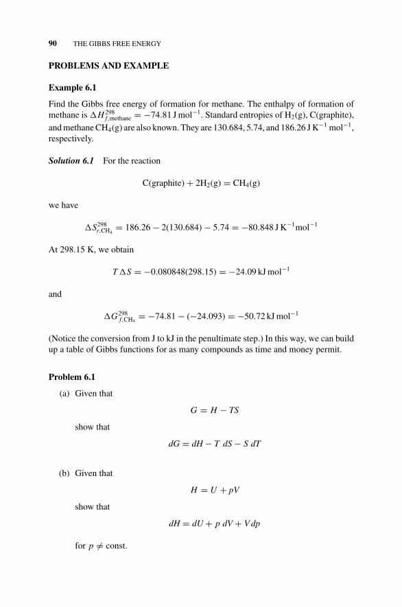
P1: OTA/XYZ P2: ABCc06 JWBS043-Rogers September 13, 2010 11:25 Printer Name: Yet to Come
90 THE GIBBS FREE ENERGY
PROBLEMS AND EXAMPLE
Example 6.1
Find the Gibbs free energy of formation for methane. The enthalpy of formation ofmethane is �H 298
f,methane = −74.81 J mol−1. Standard entropies of H2(g), C(graphite),
and methane CH4(g) are also known. They are 130.684, 5.74, and 186.26 J K−1 mol−1,respectively.
Solution 6.1 For the reaction
C(graphite) + 2H2(g) = CH4(g)
we have
�S298r,CH4
= 186.26 − 2(130.684) − 5.74 = −80.848 J K−1mol−1
At 298.15 K, we obtain
T �S = −0.080848(298.15) = −24.09 kJ mol−1
and
�G298f,CH4
= −74.81 − (−24.093) = −50.72 kJ mol−1
(Notice the conversion from J to kJ in the penultimate step.) In this way, we can buildup a table of Gibbs functions for as many compounds as time and money permit.
Problem 6.1
(a) Given that
G = H − TS
show that
dG = dH − T dS − S dT
(b) Given that
H = U + pV
show that
dH = dU + p dV + V dp
for p �= const.
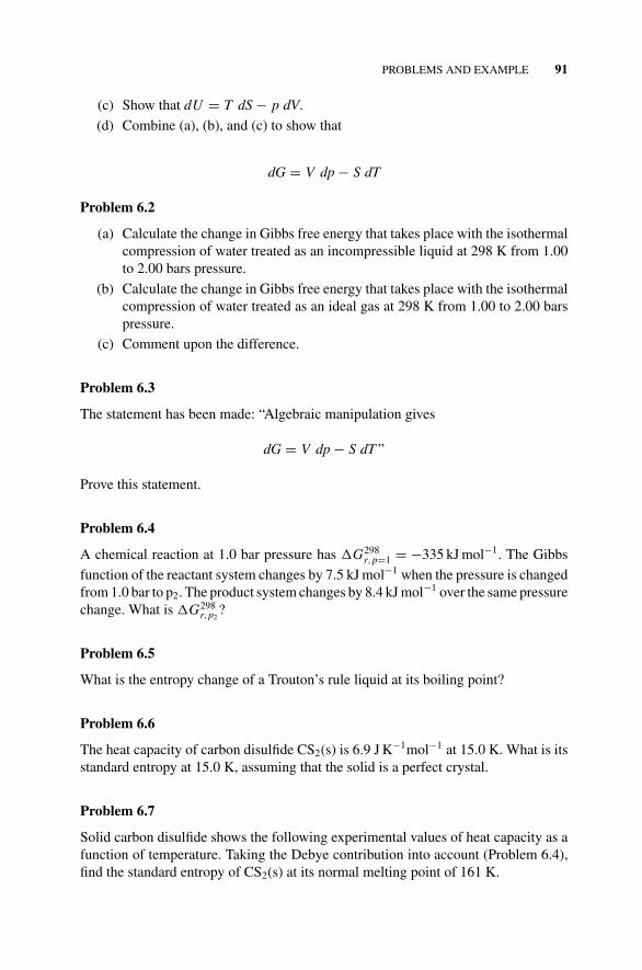
P1: OTA/XYZ P2: ABCc06 JWBS043-Rogers September 13, 2010 11:25 Printer Name: Yet to Come
PROBLEMS AND EXAMPLE 91
(c) Show that dU = T dS − p dV.
(d) Combine (a), (b), and (c) to show that
dG = V dp − S dT
Problem 6.2
(a) Calculate the change in Gibbs free energy that takes place with the isothermalcompression of water treated as an incompressible liquid at 298 K from 1.00to 2.00 bars pressure.
(b) Calculate the change in Gibbs free energy that takes place with the isothermalcompression of water treated as an ideal gas at 298 K from 1.00 to 2.00 barspressure.
(c) Comment upon the difference.
Problem 6.3
The statement has been made: “Algebraic manipulation gives
dG = V dp − S dT ”
Prove this statement.
Problem 6.4
A chemical reaction at 1.0 bar pressure has �G298r,p=1 = −335 kJ mol−1. The Gibbs
function of the reactant system changes by 7.5 kJ mol−1 when the pressure is changedfrom 1.0 bar to p2. The product system changes by 8.4 kJ mol−1 over the same pressurechange. What is �G298
r,p2?
Problem 6.5
What is the entropy change of a Trouton’s rule liquid at its boiling point?
Problem 6.6
The heat capacity of carbon disulfide CS2(s) is 6.9 J K−1mol−1 at 15.0 K. What is itsstandard entropy at 15.0 K, assuming that the solid is a perfect crystal.
Problem 6.7
Solid carbon disulfide shows the following experimental values of heat capacity as afunction of temperature. Taking the Debye contribution into account (Problem 6.4),find the standard entropy of CS2(s) at its normal melting point of 161 K.
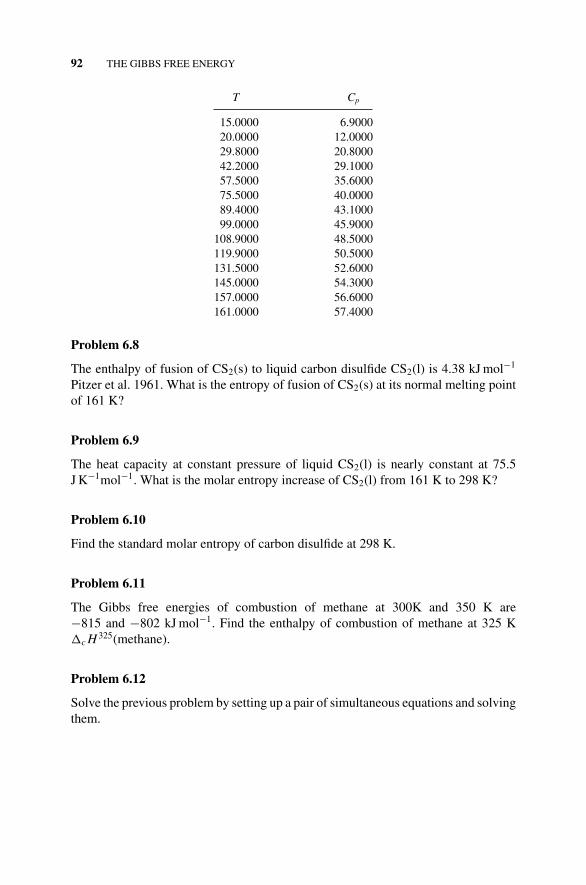
P1: OTA/XYZ P2: ABCc06 JWBS043-Rogers September 13, 2010 11:25 Printer Name: Yet to Come
92 THE GIBBS FREE ENERGY
T Cp
15.0000 6.900020.0000 12.000029.8000 20.800042.2000 29.100057.5000 35.600075.5000 40.000089.4000 43.100099.0000 45.9000
108.9000 48.5000119.9000 50.5000131.5000 52.6000145.0000 54.3000157.0000 56.6000161.0000 57.4000
Problem 6.8
The enthalpy of fusion of CS2(s) to liquid carbon disulfide CS2(l) is 4.38 kJ mol−1
Pitzer et al. 1961. What is the entropy of fusion of CS2(s) at its normal melting pointof 161 K?
Problem 6.9
The heat capacity at constant pressure of liquid CS2(l) is nearly constant at 75.5J K−1mol−1. What is the molar entropy increase of CS2(l) from 161 K to 298 K?
Problem 6.10
Find the standard molar entropy of carbon disulfide at 298 K.
Problem 6.11
The Gibbs free energies of combustion of methane at 300K and 350 K are−815 and −802 kJ mol−1. Find the enthalpy of combustion of methane at 325 K�c H 325(methane).
Problem 6.12
Solve the previous problem by setting up a pair of simultaneous equations and solvingthem.
P1: OTA/XYZ P2: ABCc07 JWBS043-Rogers September 13, 2010 11:25 Printer Name: Yet to Come
7EQUILIBRIUM
Chemists are often depicted in the popular media as sinister fellows who pour asolution from beaker A into beaker B with catastrophic results. In fact, we are neithermore nor less sinister than the next person and we take elaborate precautions to avoidcatastrophies. Nevertheless, the process of adding one or many components A of onekind to a system of another kind B to establish an equilibrium mixture is central toour art or science, and the theoretical examination of chemical equilibrium is the highpoint and culmination of classical chemical thermodynamics.
7.1 THE EQUILIBRIUM CONSTANT
Suppose that gases A and B are capable of equilibration
A(g) →← B(g)
and arbitrary amounts of A(g) and B(g) are introduced into a closed container at 298 K.Because the amounts are arbitrary, the quotient of the partial pressures Q = pB/pA
in the container will not be the equilibrium constant Keq. The chemical potentials GA
and GB will probably not be in the standard state. Instead they will differ from G◦A
and G◦B, by
GA = G◦A + RT ln
pA
1.0
Concise Physical Chemistry, by Donald W. RogersCopyright C© 2011 John Wiley & Sons, Inc.
93

P1: OTA/XYZ P2: ABCc07 JWBS043-Rogers September 13, 2010 11:25 Printer Name: Yet to Come
94 EQUILIBRIUM
and
GB = G◦B + RT ln
pB
1.0
where the 1.0 in the denominators signify that the partial pressures are relative tothe standard state of 1.0 bar. The difference between the chemical potentials of thereactant state and product state is
�r G =∑
G(prod) −∑
G(react)
which in this simple case is
�r G = GB − GA = G◦B − G◦
A + RT lnpB
1.0− RT ln
pA
1.0
or
�r G = �G◦ + RT lnpB
pA
As the reaction progresses, �r G is not zero and G of the reacting system is not constantwith time t, (∂G/∂t)T,p �= 0. When the chemical reaction has come to completion,the pressure quotient Q = pB/pA has arrived at a value such that (∂G/∂t)T,p = 0,hence
�r G = �G◦ + RT lnpB
pA= 0
The free energy change of the system has arrived at a Gibbs potential energy mini-mum. Under these and only under these conditions, we have �r G = 0, so that
�G◦ = −RT lnpB
pA= −RT ln Keq
The expression is frequently written in the equivalent form:
Keq = e−�G◦/RT
7.2 GENERAL FORMULATION
A more general formulation of the equilibrium expressions above is given by thereaction
aA + bB + . . . = cC + dD + . . .
P1: OTA/XYZ P2: ABCc07 JWBS043-Rogers September 13, 2010 11:25 Printer Name: Yet to Come
GENERAL FORMULATION 95
where a, b, . . . c, d, . . . are the stoichiometric coefficients of the reaction. It is stilltrue that
�r G =∑
G(prod) −∑
G(react)
When equilibrium has been reached, we have
�G◦ = −RT ln Keq
Now the concentration quotient Q takes the form
Q = [C]c [D]d . . .
[A]a [B]b . . .
leading to the familiar expression of the equilibrium constant as
Keq = [C]c [D]d . . .
[A]a [B]b . . .
which is true only after the Gibbs free energy has come to a minimum and �r G = 0.The stoichiometric coefficients become exponents, and the square brackets [ ] indicatesome kind of unitless concentration variable relative to a standard state. This notationis often used in solution chemistry to denote a concentration in moles/liter, where thestandard state of the solute in the solvent is taken for granted.
As an example of a reaction in the gas phase, the expression
�G◦ = −RT lnp2
NO2
pN2O4
can be used to find the equilibrium constant for the reaction
N2O4(g) →← 2NO2(g)
The standard state Gibbs chemical potential difference for this reaction is
�r G◦ = �G◦2(NO2) − �G◦
N2O4= 2(51.31) − 97.89 = 4.73 kJ mol−1
The equilibrium constant is
Keq = e−�G◦/RT = e−4730/8.314×298.15 = 0.148
which is in good agreement with the experimental value of 0.13.It is difficult to obtain accurate Keq values from calorimetric determination
of �r G◦ (from �r H ◦ and �r S◦) because of the exponential relationship Keq =e−�G◦/RT . This mathematical form brings about a large error in Keq when �r G◦ isin error by a small amount. To a certain degree, a “small” error or a “large” error isin the eye of the beholder; the terms are used in the literature as influenced by the
P1: OTA/XYZ P2: ABCc07 JWBS043-Rogers September 13, 2010 11:25 Printer Name: Yet to Come
96 EQUILIBRIUM
“difficulty” of the experiment and how “good” previous measurements of the samekind have been. Clearly, these are subjective value judgments.
7.3 THE EXTENT OF REACTION
In a chemical reaction, the participant concentrations change, but they do not changeindependently, rather they are related by the stoichiometric coefficients of the reaction.For example, if I know that reactant A decreases by 0.1 mol in the reaction system
A + B = 2C
I know that reactant B also decreases by 0.1 mol and product C increases by 0.2 mol.The infinitesimal changes in mole numbers dnA, dnB, and dnC are linearly depen-dent. One frequently expresses the change in a reaction using the single variable ξ
which, given the linear dependence of the reaction components, suffices to expressall three in the specific case cited. In general, infinitesimal variations in the amountof any number of components dni can be expressed in terms of the extent of reactionξi where
ξi = dni
νi
and νi is the stoichiometric coefficient: −1, −1, and 2 in the specific example cited.Note that the stoichiometric coefficients of the two reactants are negative becausetheir concentrations decrease as the reaction proceeds. This is a convention of course,because the reaction could equally well have been written
2C = A + B
whereupon the signs of ξi would change.Up to this point, we have stressed thermodynamic state functions for 1 mol of a
pure substance, for example, the molar energy U = f (V, T ). When we express theenergy of any mixture, specifically a mixture of reactants and products in a reactingsystem, the composition of the system in terms of mole numbers ni �= 1.0 influencesthe energy and other state functions. We can express this dependence in terms of theextent of reaction:
U = f (V, T, ξi )
This dependence means that along with V and T , ξi is a full-fledged degree of freedomand we can write the exact differential
dU =(
∂U
∂V
)T,ξi
dV +(
∂U
∂T
)V,ξi
dT +(
∂U
∂ξi
)T,V
dξi + . . .
where i extends over all degrees of freedom.
P1: OTA/XYZ P2: ABCc07 JWBS043-Rogers September 13, 2010 11:25 Printer Name: Yet to Come
VARIATION OF THE EQUILIBRIUM CONSTANT WITH TEMPERATURE 97
Notice that this implies a hyperspace in U, V, T, and ξi . Energy has been selectedhere to illustrate the principle that analogous equations exist for the other statevariables—for example, G, H, and S.
7.4 FUGACITY AND ACTIVITY
For nonideal systems the concentration variable is replaced by a new variable thatexpresses the effective concentration of the species in a mixture. For example, a solutemay be more chemically active in methanol solution than it is in water. Or it may bemore active in water solution than in methanol. A pure gas may behave in a nonidealway, and its degree of nonideality may be influenced by other gases in a mixture.These deviations from ideal behavior are expressed by a coefficient γ which yieldsthe activity of a solute or fugacity of a gas when multiplied into the concentrationvariable, for example,
aA = γA [A] or fA = γA pA
The activity and fugacity coefficients are simply numbers telling us whether thebehavior of the species is greater or less than it would be in the standard state. Theyare concentration- or pressure-dependent and are usually determined for real systemsby rather painstaking empirical methods.
7.5 VARIATION OF THE EQUILIBRIUM CONSTANTWITH TEMPERATURE
Combining the Gibbs–Helmholtz equation for the temperature variation of free energywith the equation connecting the free energy in the standard state to the equilibriumconstant gives
⎡⎢⎢⎣
∂
(�G◦
T
)
∂
(1
T
)⎤⎥⎥⎦
p
=
⎡⎢⎢⎣
∂
(−RT ln Keq
T
)
∂
(1
T
)⎤⎥⎥⎦
p
= −
⎡⎢⎢⎣∂
(R ln Keq
)∂
(1
T
)⎤⎥⎥⎦
p
but
⎡⎢⎢⎣
∂
(�G◦
T
)
∂
(1
T
)⎤⎥⎥⎦
p
= �H ◦
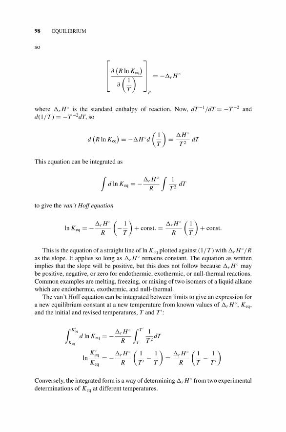
P1: OTA/XYZ P2: ABCc07 JWBS043-Rogers September 13, 2010 11:25 Printer Name: Yet to Come
98 EQUILIBRIUM
so
⎡⎢⎢⎣∂
(R ln Keq
)∂
(1
T
)⎤⎥⎥⎦
p
= −�r H ◦
where �r H ◦ is the standard enthalpy of reaction. Now, dT −1/dT = −T −2 andd(1/T ) = −T −2dT, so
d(R ln Keq
) = −�H ◦d
(1
T
)= �H ◦
T 2dT
This equation can be integrated as
∫d ln Keq = −�r H ◦
R
∫1
T 2dT
to give the van’t Hoff equation
ln Keq = −�r H ◦
R
(− 1
T
)+ const. = �r H ◦
R
(1
T
)+ const.
This is the equation of a straight line of ln Keq plotted against (1/T ) with �r H ◦/Ras the slope. It applies so long as �r H ◦ remains constant. The equation as writtenimplies that the slope will be positive, but this does not follow because �r H ◦ maybe positive, negative, or zero for endothermic, exothermic, or null-thermal reactions.Common examples are melting, freezing, or mixing of two isomers of a liquid alkanewhich are endothermic, exothermic, and null-thermal.
The van’t Hoff equation can be integrated between limits to give an expression fora new equilibrium constant at a new temperature from known values of �r H ◦, Keq,and the initial and revised temperatures, T and T ′:
∫ K ′eq
Keq
d ln Keq = −�r H ◦
R
∫ T ′
T
1
T 2dT
lnK ′
eq
Keq= −�r H ◦
R
(1
T ′ − 1
T
)= �r H ◦
R
(1
T− 1
T ′
)
Conversely, the integrated form is a way of determining �r H ◦ from two experimentaldeterminations of Keq at different temperatures.

P1: OTA/XYZ P2: ABCc07 JWBS043-Rogers September 13, 2010 11:25 Printer Name: Yet to Come
VARIATION OF THE EQUILIBRIUM CONSTANT WITH TEMPERATURE 99
7.5.1 Le Chatelier’s Principle
Le Chatelier’s principle states that, in a stressed chemical reaction, the equilibriumwill be displaced in such a way as to relieve the stress. First, we need to define“stress.” An exothermic reaction
A →← B + q
where q is heat given off, will be stressed backward by application of heat q—thatis, by a temperature rise. Application of heat will drive the reaction backward to givemore A and less B. The opposite will be true for an endothermic reaction. Lookingat the integrated van’t Hoff equation
lnK ′
eq
Keq= �r H ◦
R
(1
T− 1
T ′
)
we see that for a temperature rise T ′ > T we have (1/T ) > (1/T ′). For �r H ◦ < 0,ln (K ′
eq/Keq) < 0 and the new equilibrium constant K ′eq is smaller than the original
one, Keq. The thermal condition �r H ◦ < 0 is the characteristic of an exothermicreaction, so Le Chatelier’s principle applied to the heat of reaction agrees with thevan’t Hoff equation. Le Chatelier’s principle is a qualitative statement giving thesign but not the magnitude of the effect of a temperature change on the equilibriumconstant.
7.5.2 Entropy from the van’t Hoff Equation
If �r H ◦ is independent of the temperature, then from d�r H ◦ = �r C p dT = 0. SincedT is not zero, �r C p must be zero. From
�r C p =∑
C p(prod) −∑
C p(react)
the heat capacity of the reactant system must be equal to that of the product system. Inpractical terms, we take this equality to be approximately true over short temperatureintervals. We have already found the equations
�r G◦ = −RT ln Keq
and
�r G◦ = �r H ◦ − T �r S◦
so
−RT ln Keq = �r H ◦ − T �r S◦
P1: OTA/XYZ P2: ABCc07 JWBS043-Rogers September 13, 2010 11:25 Printer Name: Yet to Come
100 EQUILIBRIUM
and
ln Keq = −�r H ◦
R
(1
T
)+ �r S◦
R
This is a “slope–intercept” problem for the linear function ln Keq vs. 1/T , where theslope of the plot is −�r H ◦/R and the intercept is �r S◦/R. Two or more equilibriummeasurements at different temperatures yield both the enthalpy change of the reactionand the entropy change. The resulting thermodynamic functions are only as good asthe input data, and this is a very sensitive experimental problem—especially in the�r S◦ determination, which depends on what may be a long and mathematicallyquestionable extrapolation.
7.6 COMPUTATIONAL THERMOCHEMISTRY
Within a year of the discovery of quantum mechanics by Schrodinger and Heisenberg,Heitler and London had demonstrated that the energy of the H H chemical bond canbe approximated by a quantum mechanical calculation. The reason this calculationis always approximate is a reflection of one of the most profound laws of nature,Heisenberg’s uncertainty principle. We are unable to know exactly where the movingelectrons are. Hence their Coulombic potential energy, total energy, entropy, andGibbs free energy are inaccessible to us in even the simplest chemical bond H H.
Nevertheless, a diverse array of approximate computational methods exists andthe results can be ranked in order of the quality of their approximations. Rankingenables us to decide which methods are best for a given job, and it points theway toward improved methods. Usually the quality of an approximate calculation ismeasured by how well the calculated value matches well-established experimentalresults. Recently, however, computed values have become so reliable that they can beused to pick out and discard errors in the tabulated experimental results. The presenttrend is from using computed results to approximate experimental results to usingthem to supplant or replace experimental results, especially for reactions that occurwithin hostile experimental environments (flames or explosions) or reactions thathave fleeting intermediates (free radicals). Quantum mechanical methods produceresults for molecular energy, enthalpy, entropy, Gibbs free energy, and equilibriumconstants, but they are circumscribed by limits on molecular size and they are ofvarying reliability.
7.7 CHEMICAL POTENTIAL: NONIDEAL SYSTEMS
Given that the effective pressure fraction of a gas in a nonideal mixture of gases isits fugacity f and that the effective concentration fraction of a solute in a mixture isgiven by its activity a, equilibrium constants in simple A, B nonideal systems can be
P1: OTA/XYZ P2: ABCc07 JWBS043-Rogers September 13, 2010 11:25 Printer Name: Yet to Come
CHEMICAL POTENTIAL: NONIDEAL SYSTEMS 101
written
Keq = fB
fAor Keq = aB
aA
The Gibbs free energy of a pure substance is a function of the temperature andpressure only, G = g(T, p), but the free energy of a many-component system is afunction of T , p, and the amounts of each component ni , G = g(T, p, ni ). The totalchange in free energy for a mixture is
dG =(
dG
dT
)p,ni
dT +(
dG
dp
)T,ni
dp +∑
i
(dG
dni
)p,T
dni
It is the last term that we are interested in. At constant T and p, we have
dG =∑
i
(dG
dni
)p,T
dni
where the n j are constant ( j �= i). In the simple illustrative reaction mixture,
A(g) →← B(g)
in the ideal case,
�G = �G◦ + RT ln Q = �G◦ + RT lnpB
pA
where the p values are partial pressures. In the nonideal case the form of the pressurequotient Q still holds, but the partial pressures are replaced by the fugacities f . Thechange in the Gibbs free energy is also given a different symbol �µ to denote thenonideal case:
�µ = �µ◦ + RT ln Q = �µ◦ + RT lnfB
fA
Evidently,
�µ = µB − µA
and
�µ◦ = µ◦B − µ◦
A
P1: OTA/XYZ P2: ABCc07 JWBS043-Rogers September 13, 2010 11:25 Printer Name: Yet to Come
102 EQUILIBRIUM
Although the Gibbs chemical potential applies to the many-component nonideal caseas well as the ideal case, it is mathematically rigorous and it is a thermodynamicfunction.
From these definitions of the Gibbs chemical potentials, it follows that
µA = µ◦A + RT ln fA
and
µB = µ◦B + RT ln fB
In the general case, Gibbs chemical potentials are
µi = µ◦i + RT ln fi
for an indefinite number of fugacities.Analogous definitions for the general case lead to
µi = µ◦i + RT ln ai
for activities ai, with
Q = [C]c [D]d . . .
[A]a [B]b . . .=
∏i
[X ]i
∏j
[X ] j
where the [X ]i and [X ] j are relative concentration variables, pressure fractions, molefractions, mass fractions, and so on, symbolized by either f or a and taken to theappropriate stoichiometric coefficient.
7.8 FREE ENERGY AND EQUILIBRIA IN BIOCHEMICAL SYSTEMS
Reactions of biochemical interest do not normally occur in the gas phase. Ratherthey occur in solution, usually saline solution. Therefore the correct expressionof the free energy changes of reaction and the equilibrium constant is in termsof the corresponding activities and changes in chemical potential. Determination ofactivities and activity coefficients over a concentration range on nonideal solutions isnot a simple matter, nor is it necessary for in vitro studies of biochemical reactions.Instead, concentrations are used with the stipulation that the “background” condi-tions must be constant over the course of the study and must be reproduced from onestudy to the next. For example, energy studies on dephosphorylation of adenosine
P1: OTA/XYZ P2: ABCc07 JWBS043-Rogers September 13, 2010 11:25 Printer Name: Yet to Come
FREE ENERGY AND EQUILIBRIA IN BIOCHEMICAL SYSTEMS 103
5′-triphosphate would be carried out at a specified and constant temperature, pres-sure, pH, pMg, and ionic strength where pH and pMg refer to the ion concentrationspH = − log
[H+]
and pMg = − log[Mg2+]
, and the ionic strength is constant for alldissolved salts in the reaction solution. Ionic strength is essentially the ionic chargeconcentration in solution calculated as the sum 1
2
∑ci z2
i over all salt concentrationsci that dissolve to give ions of charge zi .
These conditions specify a unique standard state which is not the thermodynamicstandard state but which is adhered to throughout the experiment and experimentswith which results will be combined or compared. Under these controls, it is properto write
GA = G◦A + RT ln [A]
for G◦A in the specified standard state with a concentration of reactant A, with similar
expressions for B, C, . . . . The change in free energy for a reaction quotient Q, nowin terms of initial concentrations, is
�G = �G◦ + RT ln Q = �G◦ + RT ln[C]ξ [D]ξ . . .
[A]ξ [B]ξ . . .
Different stoichiometric coefficients are all expressed using the same symbol ξ forsimplicity. It is understood that Q is a concentration quotient, which might fortuitouslybe equal to the equilibrium constant but in general will not. In general, �G will bedifferent from zero but when the reaction has arrived at equilibrium, the concentrationswill have arrived at Keq and �G will have arrived at zero so that
�G◦ = −RT ln Keq
Thus the form of the free energy relation to the equilibrium constant is reproduced butonly under rigorously controlled background conditions.1 Change the ionic strengthor the pH, for example, and you can expect to find a different �G◦ and Keq.
How can �G◦ change when we usually think of it as a sum of rock-firm G◦
values? By changing our background conditions, we have changed the standard state,the benchmark to which we refer all G◦ values.
7.8.1 Making ATP, the Cell’s Power Supply
The difference between �r G and �G◦ in the metabolic degradation of glucose,a physiological energy source, to lactate and ATP can be broken down into twoindividual steps (Hammes, 2007), one taking up 2 mol of ATP and producing 2 molof the diphosphate ADP
Glucose + 2 ATP → 2 ADP + 2 glyceraldehyde-3-phosphate
1See Treptow (1996).
P1: OTA/XYZ P2: ABCc07 JWBS043-Rogers September 13, 2010 11:25 Printer Name: Yet to Come
104 EQUILIBRIUM
and the other producing 4 mol of ATP
2 Glyceraldehyde-3-phosphate + 2 phosphate + 4 ADP → 2 lactate + 4 ATP + 2 H2O
The summed reaction is
Glucose + 2 phosphate + 2 ADP → 2 lactate + 2 ATP + 2 H2O
for a net gain of 2 mol of ATP. The first of these two reactions is unfavorable fromthe point of view of a positive �G◦ = 2.2 kJ mol−1 but at the initial concentrationschosen to be at or near physiological concentrations,
Q = (0.14)2 (0.019)2
5.0 (1.85)2 = 0.0196(3.61 × 10⁻⁴
) ≈ 4 × 10⁻⁷ � 1
This very small reaction quotient drives the metabolic conversion of ADP to ATPwhich then powers other reactions within the biological system as a whole.
PROBLEMS AND EXAMPLES
Example 7.1 Solution Calorimetry
A half-liter solution calorimeter system consisted of the calorimeter itself, a tempera-ture measuring circuit, an electrical heating circuit, and calorimeter fluid. The systemwas prepared with a solution of magnesium ion at 0.001 M. The ionic strength wasbrought to 0.25 M with KCl, a neutral electrolyte, and the pH was adjusted to 7.0.When the heating circuit was activated at a current flow of I amperes for a time t,an amount of heat energy qp = 96.5 J was delivered through a heating resistor R(q = I 2 Rt) producing a temperature rise of �T = 0.166 K.2 What was the waterequivalent (calorimeter constant) of the calorimeter system?
Solution to Example 7.1 The water equivalent of a calorimeter is the heat capacityof the entire system as if it were all water even though it consists of various parts madeof various materials and contains a solution of reactants and products different frompure water. The water equivalent can be found by a straightforward heat capacitycalculation even though we know that the heat capacity of the system is the sum ofmany parts. We calculate
C p = dqp
dT qp
�T= 95.6
0.166= 576 J K−1 = 0.576 kJ K−1
21 amp volt sec = 1 J and E in volts = IR.
P1: OTA/XYZ P2: ABCc07 JWBS043-Rogers September 13, 2010 11:25 Printer Name: Yet to Come
PROBLEMS AND EXAMPLES 105
Example 7.2 Adenosine 5′-triphosphate ATP
The hydrolysis of adenosine 5′-triphosphate ATP to adenosine 5′-diphosphate ADPplus an inorganic phosphate ion can be written
ATP + H2O → ADP + phosphate
If 10 mL of ATP with concentration [ATP] = 0.200 mol L−1are pipetted into acalorimeter with a heat capacity of 0.576 kJ K−1 (Example 7.1) and a temperature riseof 0.107 K is found, what is the enthalpy of hydrolysis of adenosine 5′-triphosphateto adenosine 5′-diphosphate plus an inorganic phosphate ion under these conditions?What is the sign of �r H?
Solution to Example 7.2
0.107 K(0.576 kJ K−1
) = 0.0616 kJ
10.0 mL = 0.0100 L
0.0100 L(0.200 mol L−1) = 0.00200 mol ATP
0.0616 kJ
0.00200 mol= −30.8 kJ mol−1
The sign of �r H is negative because the reaction is exothermic. Heat flowing outof the reacting system at constant external pressure means that its enthalpy balancemust decrease.
Problem 7.1
What is the change in the entropy S for one mole of a pure substance for an infinites-imal change in T and p? Given: Entropy is an exact differential
d S(T, p) =(
∂S
∂T
)p
dT +(
∂S
∂p
)T
dp
Problem 7.2
In an experiment on the nitrogen tetroxide reaction at 298 K
N2O4(g) →← 2NO2(g)
pure N2O4(g) was introduced into a reaction vessel maintained at constant temperatureand a total pressure of 2.500 bar. When equilibrium had been reached, the partial
P1: OTA/XYZ P2: ABCc07 JWBS043-Rogers September 13, 2010 11:25 Printer Name: Yet to Come
106 EQUILIBRIUM
pressure of N2O4(g) had dropped to 1.975 bar. What is Keq for this reaction? Compareyour answer to the calculated value (Section 7.2). What are the units of Keq?
Problem 7.3
Supposing that a simple A(g) →← B(g) reaction has an equilibrium constant Keq =0.100 at T = 200 K and K ′
eq = 0.200 at T = 300 K. What is �r H ◦ for the reaction?
Problem 7.4
For the reaction
Br2(g) → 2Br(g)
the equilibrium constant has been measured and found to be 0.410 at 1125 K and1.40 at 1175 K. What is Keq at 1225 K?
Problem 7.5
Data quoted in Lewis and Randall (1961) for the formation reaction of H2S
H2(g) + 12 S2(g) = H2S(g)
include the values given in Table 7.1.
TABLE 7.1 T, 1/T, K, and ln K for formation of H2S from its elements.
T 1023 1218 1405 16671/T 9.775 × 10⁻⁴ 8.210 × 10⁻⁴ 7.117 × 10⁻⁴ 5.999 × 10⁻⁴
K 105.9 20.18 6.209 1.807ln K 4.662 3.005 1.826 0.5917
What is �r H ◦ for this reaction? What is �r S◦?
Problem 7.6
A reaction in the gas phase has Keq = 10 at 298 K and 10−1 at 500 K. Is the reactionendothermic or exothermic? Explain this in terms of Le Chatelier’s principle.
Problem 7.7
An experiment was set up so that conditions (pH, pMg+, ionic strength, etc.) wereidentical to those described in Exercises 7.1 and 7.2, except that, in this experiment,

P1: OTA/XYZ P2: ABCc07 JWBS043-Rogers September 13, 2010 11:25 Printer Name: Yet to Come
PROBLEMS AND EXAMPLES 107
adenosine 5′-diphosphate ADP was substituted for ATP. The hydrolysis reactionproducing adenosine 5′-monophosphate AMP
ADP + H2O → ADP + phosphate
resulted in a temperature change of �T = 0.100 K. Find �H ◦ for the reaction
2ADP → AMP + ATP
(The symbol �H ◦ is used to indicate a standard enthalpy change relative to a definedconcentration under specific solution conditions.)
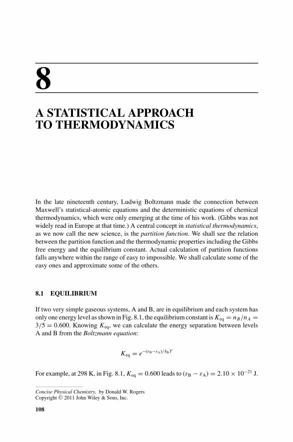
P1: OTA/XYZ P2: ABCc08 JWBS043-Rogers September 13, 2010 11:25 Printer Name: Yet to Come
8A STATISTICAL APPROACHTO THERMODYNAMICS
In the late nineteenth century, Ludwig Boltzmann made the connection betweenMaxwell’s statistical-atomic equations and the deterministic equations of chemicalthermodynamics, which were only emerging at the time of his work. (Gibbs was notwidely read in Europe at that time.) A central concept in statistical thermodynamics,as we now call the new science, is the partition function. We shall see the relationbetween the partition function and the thermodynamic properties including the Gibbsfree energy and the equilibrium constant. Actual calculation of partition functionsfalls anywhere within the range of easy to impossible. We shall calculate some of theeasy ones and approximate some of the others.
8.1 EQUILIBRIUM
If two very simple gaseous systems, A and B, are in equilibrium and each system hasonly one energy level as shown in Fig. 8.1, the equilibrium constant is Keq = nB/n A =3/5 = 0.600. Knowing Keq, we can calculate the energy separation between levelsA and B from the Boltzmann equation:
Keq = e−(εB−εA)/kBT
For example, at 298 K, in Fig. 8.1, Keq = 0.600 leads to (εB − εA) = 2.10 × 10⁻²¹ J.
Concise Physical Chemistry, by Donald W. RogersCopyright C© 2011 John Wiley & Sons, Inc.
108

P1: OTA/XYZ P2: ABCc08 JWBS043-Rogers September 13, 2010 11:25 Printer Name: Yet to Come
DEGENERACY AND EQUILIBRIUM 109
B(g)A(g)
· · · Bε
· · · · · Aε
FIGURE 8.1 A two-level equilibrium. There are 5 molecules in A and 3 molecules in B.
Conversely, knowing the energy separation, one can calculate the equilibriumconstant. If the energy of B is lower than the energy of A by 2.10 × 10⁻²¹J, level Bwill contain more molecules at equilibrium than will level A and Keq will be largerthan 1.0 (Fig. 8.2).
Keq = nB
nA= e−(εB−εA)/kBT = 5
3= 1.67
In these simple models, the equilibrium constants are inverses and (εB − εA) of thefirst equilibrium is equal but opposite in sign to (εB − εA) of the second reaction. Thisanalysis gives a description of the relationship between energy and the equilibriumconstant that is useful as far as it goes, but it has left out an important consideration:the influence of entropy.
8.2 DEGENERACY AND EQUILIBRIUM
If the upper level is split into two levels, each of which has the same energy, itscapacity to accommodate molecules of kind B is doubled (Fig. 8.3). The equilibrium
constant Keq = 6
5has been made greater than 1.0. The reaction now favors products
rather than reactants even though the energy change is uphill. The second law hascome into play; the product state is more disordered. There are more places for themolecule to go. It is like having two stacks of paper on your desk rather than one.There are now two places where that important piece of paper you are looking for maybe, whereas before there was only one. Increased disorder means increased entropy.
· · ·
· · · · ·
B A
FIGURE 8.2 A two-level equilibrium.
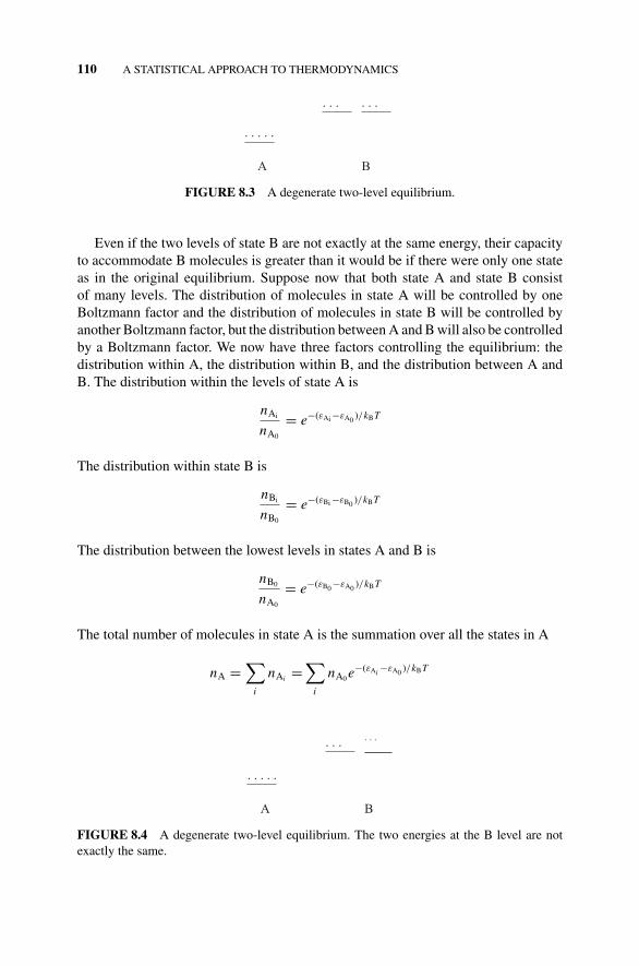
P1: OTA/XYZ P2: ABCc08 JWBS043-Rogers September 13, 2010 11:25 Printer Name: Yet to Come
110 A STATISTICAL APPROACH TO THERMODYNAMICS
· · · · · ·
· · · · ·
B A
FIGURE 8.3 A degenerate two-level equilibrium.
Even if the two levels of state B are not exactly at the same energy, their capacityto accommodate B molecules is greater than it would be if there were only one stateas in the original equilibrium. Suppose now that both state A and state B consistof many levels. The distribution of molecules in state A will be controlled by oneBoltzmann factor and the distribution of molecules in state B will be controlled byanother Boltzmann factor, but the distribution between A and B will also be controlledby a Boltzmann factor. We now have three factors controlling the equilibrium: thedistribution within A, the distribution within B, and the distribution between A andB. The distribution within the levels of state A is
nAi
nA0
= e−(εAi −εA0 )/kBT
The distribution within state B is
nBi
nB0
= e−(εBi −εB0 )/kBT
The distribution between the lowest levels in states A and B is
nB0
nA0
= e−(εB0 −εA0 )/kBT
The total number of molecules in state A is the summation over all the states in A
nA =∑
i
nAi =∑
i
nA0 e−(εAi −εA0 )/kBT
· · · · · ·
· · · · ·
B A
FIGURE 8.4 A degenerate two-level equilibrium. The two energies at the B level are notexactly the same.
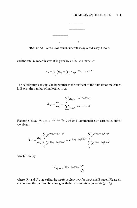
P1: OTA/XYZ P2: ABCc08 JWBS043-Rogers September 13, 2010 11:25 Printer Name: Yet to Come
DEGENERACY AND EQUILIBRIUM 111
==========
==========
==========
B A
FIGURE 8.5 A two-level equilibrium with many A and many B levels.
and the total number in state B is given by a similar summation
nB =∑
i
nBi =∑
i
nB0 e−(εBi −εB0 )/kBT
The equilibrium constant can be written as the quotient of the number of moleculesin B over the number of molecules in A:
Keq = nB
nA=
∑i
nB0 e−(εBi −εB0 )/kBT
∑i
nA0 e−(εAi −εA0 )/kT
Factoring out nB0/nA0 = e−(εB0 −εA0 )/kBT , which is common to each term in the sums,we obtain
Keq = nB0
nA0
∑i
e−(εBi −εB0 )/kBT
∑i
e−(εAi −εA0 )/kBT= e−(εB0 −εA0 )/kBT
∑i
e−(εBi −εB0 )/kBT
∑i
e−(εAi −εA0 )/kBT
which is to say
Keq = e−(εB0 −εA0 )/kBT Q B
Q A
where Q A and Q B are called the partition functions for the A and B states. Please donot confuse the partition function Q with the concentration quotients Q or Q.
P1: OTA/XYZ P2: ABCc08 JWBS043-Rogers September 13, 2010 11:25 Printer Name: Yet to Come
112 A STATISTICAL APPROACH TO THERMODYNAMICS
8.3 GIBBS FREE ENERGY AND THE PARTITION FUNCTION
Taking logarithms of the previous equation, we obtain
ln Keq = −�ε0
RT+ ln
Q B
Q A
where �ε0 = εB0 − εA0 . Multiplying by −RT , we get
−RT ln Keq = �ε0 − RT lnQ B
Q A
but −RT ln Keq = �G◦, so
�G◦ = �ε0 − RT lnQ B
Q A
Comparing this equation with the definition of the Gibbs chemical potential�G◦ ≡ �H ◦ − T �S◦, we see that the classical enthalpy change �H ◦ for a re-action is largely controlled by the energy separating the ground states �ε0, and theentropy change T �S◦ is largely controlled by the ratio of the multiplicity of levelsavailable in each state RT ln (Q B/Q A). In very many cases, the enthalpy change isdominant in chemical reactions, which explains why some very good nineteenth-century scientists thought that �H ◦ was the only factor controlling equilibrium andreaction spontaneity.
Given that reactions and physical processes exist that are not solely controlled ordominated by the enthalpy change, it is the ratio of partition functions that interestsus. The partition function gives us the distribution of molecules over the energy levelswithin a state. We may think of these as microstates within a state. If the enthalpybalance is close, the reaction tends to go in the direction with the most microstates.Such a reaction or process is maximizing the number of choices a particle (molecule)has in which to reside within a state. A system providing a maximum number ofchoices provides the maximum disorder, just as the number of places you may findthat piece of paper you are looking for is determined by the disorder of the desktop.A disordered desktop has more microstates than an orderly one.
Looking again at the equation �G◦ = �ε0 − RT ln (Q B/Q A), we can see anotherreason why thermodynamicists prior to Gibbs could have missed the importance ofentropy in equilibrium. The second term includes T , so it may be small at ordinarytemperatures. The ratio of microstates QB/QA may be negligible at lower tempera-tures, but it becomes important at higher temperatures and it may favor or disfavorthe product side of the equilibrium according to which is larger, QA or QB. As istrue in classical thermodynamics, there are four possibilities for the two terms in�G◦ = �ε0 − RT ln (Q B/Q A): They may be FF, FD, DF, or DD, where F denotesa term that favors the product side of the equilibrium and D denotes a term thatdisfavors the product side.
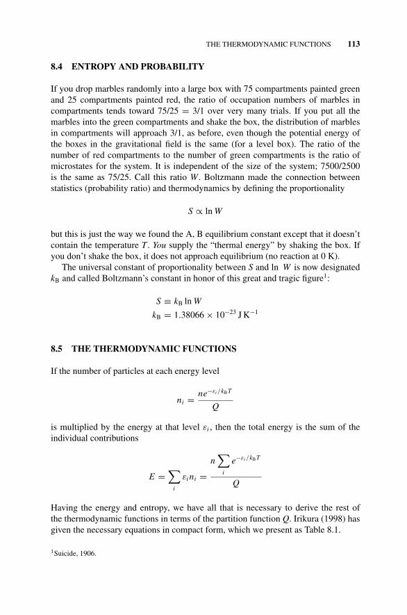
P1: OTA/XYZ P2: ABCc08 JWBS043-Rogers September 13, 2010 11:25 Printer Name: Yet to Come
THE THERMODYNAMIC FUNCTIONS 113
8.4 ENTROPY AND PROBABILITY
If you drop marbles randomly into a large box with 75 compartments painted greenand 25 compartments painted red, the ratio of occupation numbers of marbles incompartments tends toward 75/25 = 3/1 over very many trials. If you put all themarbles into the green compartments and shake the box, the distribution of marblesin compartments will approach 3/1, as before, even though the potential energy ofthe boxes in the gravitational field is the same (for a level box). The ratio of thenumber of red compartments to the number of green compartments is the ratio ofmicrostates for the system. It is independent of the size of the system; 7500/2500is the same as 75/25. Call this ratio W. Boltzmann made the connection betweenstatistics (probability ratio) and thermodynamics by defining the proportionality
S ∝ ln W
but this is just the way we found the A, B equilibrium constant except that it doesn’tcontain the temperature T . You supply the “thermal energy” by shaking the box. Ifyou don’t shake the box, it does not approach equilibrium (no reaction at 0 K).
The universal constant of proportionality between S and ln W is now designatedkB and called Boltzmann’s constant in honor of this great and tragic figure1:
S ≡ kB ln W
kB = 1.38066 × 10⁻²³ J K−1
8.5 THE THERMODYNAMIC FUNCTIONS
If the number of particles at each energy level
ni = ne−εi /kBT
Q
is multiplied by the energy at that level εi , then the total energy is the sum of theindividual contributions
E =∑
i
εi ni =n
∑i
e−εi /kBT
Q
Having the energy and entropy, we have all that is necessary to derive the rest ofthe thermodynamic functions in terms of the partition function Q. Irikura (1998) hasgiven the necessary equations in compact form, which we present as Table 8.1.
1Suicide, 1906.

P1: OTA/XYZ P2: ABCc08 JWBS043-Rogers September 13, 2010 11:25 Printer Name: Yet to Come
114 A STATISTICAL APPROACH TO THERMODYNAMICS
TABLE 8.1 Thermodynamic Functions(Irikura, 1998).
S = NkB
[∂
∂T(T ln Q) − ln N + 1
]
CV = NkBT∂2
∂T 2(T ln Q)
Cp = CV + R
H (t) − H (0) =∫ T
0CpdT = RT 2
Q
∂ Q
∂T+ RT
∂
∂T(T ln Q) = ln Q + T
Q
∂ Q
∂T
∂2
∂T 2(T ln Q) = 2
Q
∂ Q
∂T+ T
Q
∂2 Q
∂T 2− T
Q2
(∂ Q
∂T
)2
∂ Q
∂T= 1
kBT 2
∑i
εi e−εi /kBT
∂2 Q
∂T 2= −2
T
∂ Q
∂T+ 1
k2BT 4
∑i
ε2i e−εi /kBT
The essential thermodynamic functions are expressed above the line in Table 8.1,and the derivatives are given below the line for somewhat simpler and more practicalevaluation. Along with the equations in Table 8.1, “excess” free energy and enthalpyfunctions are defined as (G◦ − H0)/T and (H ◦ − H0)/T . The excess thermodynamicproperty is the amount of that quantity above the value per degree K the system wouldhave if all its parts were in the lowest possible energy state. Excess free energy andenthalpy functions vary in a gradual way over a wide range of temperature T . Thisenables one to make accurate interpolations and to extrapolate from data one has toget information one does not have.
Now we need to find out how to calculate the partition function.
8.6 THE PARTITION FUNCTION OF A SIMPLE SYSTEM
Spectroscopy gives information as to the intervals between energy levels in molecules,hence it is a gateway to molecular partition functions. As a simple example, considera noninteracting2 system of chemical bonds treated as harmonic oscillators (Chap-ter 18). A harmonic oscillator has the peculiar property that its energy levels are
2Strictly, the system is weakly interacting because particle transfer from one level to another is a necessarycondition of the statistical treatment.

P1: OTA/XYZ P2: ABCc08 JWBS043-Rogers September 13, 2010 11:25 Printer Name: Yet to Come
THE PARTITION FUNCTION OF A SIMPLE SYSTEM 115
equally spaced. Because of this, the sum, written without degeneracy,
Qvib =∑
i
e−εi /kBT , i = 0, 1, 2, . . .
can be represented by
Qvib = 1 + e−ε/kBT + e−2ε/kBT + e−3ε/kBT + · · ·
where ε is the size of equal steps up an energy ladder. Multiplying both sides of thisequation by e−ε/kBT , we get
e−ε/kBT Qvib = e−ε/kBT + e−2ε/kBT + e−3ε/kBT + · · ·
but this sum is the same as the one above it except that it lacks the first term. Thedifference between the two sums is just unity:
Qvib − e−ε/kBT Qvib = 1
so
Qvib = 1
1 − e−ε/kBT
An ideal harmonic oscillator has only one vibrational spectral line at frequency ν,which gives its energy through the Planck equation ε = hν, where h is Planck’sconstant 6.626 × 10⁻³⁴ J s. Knowing the energy ε for the oscillator, one knows Qvib.
Spectroscopists give the frequency of vibration as ν in units of reciprocal cm, cm−1.Converting this unit to ν, we have ν = c ν where c is the speed of electromagneticradiation, 3.00 × 10⁸ m s−1. The formula for Qvib in spectrocopist’s terms is
Qvib = 1
1 − e−ε/kBT= 1
1 − e−hcνβ= 1
1 − e−a
where β = 1/kBT and constants have been gathered for convenience into
a = 1.439ν
T
The diatomic molecule Na2(g) at 1000 K, for example, has a strong vibrationalresonance at 159.2 cm−1. This leads to a = 1.439(159.2)/1000 = 0.229 and
Qvib = 1
1 − e−0.229= 4.88

P1: OTA/XYZ P2: ABCc08 JWBS043-Rogers September 13, 2010 11:25 Printer Name: Yet to Come
116 A STATISTICAL APPROACH TO THERMODYNAMICS
Similarly, the rotational partition function Qrot, in spectroscopist’s terms is
Qrot = 1
hcBβ= 0.695T
σ B
where B is the rotational resonance frequency, again in units of cm−1, and σ isa “symmetry number” included to take into account the fact that a symmetricalmolecule has different configurations that are, from a geometric point of view, thesame. For example, the linear molecule Na–Na rotated by one half a rotation isstill just Na–Na, indistinguishable from the starting configuration. The differencebetween distinguishable and indistinguishable configurations changes the statisticsof the problem. (The statistics of a poker game using a deck in which each ace hasan identical twin is not the same as the statistics using an honest deck.)
The rotational resonance frequency of interest for Na2(g) is B = 0.1547 cm−1.Applying the spectroscopist’s formula to the Na–Na molecule with its symmetrynumber of 2 gives
Qrot = 0.695T
σ B= 0.695(1000)
2(0.1547)= 2246
This kind of calculation will be useful to us in Section 8.8. Further discussion of Qdetermination is given in more detailed works (Nash, 2006; Maczek, 1998).
8.7 THE PARTITION FUNCTION FOR DIFFERENT MODESOF MOTION
A molecule can absorb energy by increasing its translational motion (displacementof the entire molecule), increasing its rotational motion, and increasing its vibrationalmotion, as well as by electronic excitation. The total energy of a molecule is the sumof energy contributions from all of its modes of motion:
ε = εtr + εrot + εvib + εel
In terms of its different modes of motion, the partition function is
Q =∑
i
e−(εtr+εrot+εvib+εel)/kBT
Exponential sums can be written as products ea+b = eaeb, and so on, so Q can bebroken up into contributing partition functions, one for each mode of motion:
Q =∑
i
e−(εtr)/kBT∑
i
e−(εrot)/kBT∑
i
e−(εvib)/kBT∑
i
e−(εel )/kBT
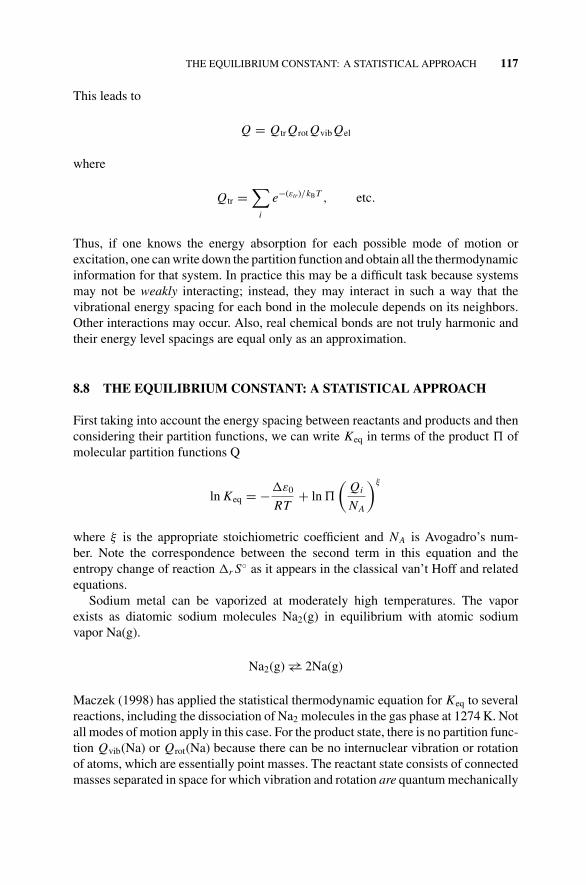
P1: OTA/XYZ P2: ABCc08 JWBS043-Rogers September 13, 2010 11:25 Printer Name: Yet to Come
THE EQUILIBRIUM CONSTANT: A STATISTICAL APPROACH 117
This leads to
Q = Qtr Qrot Qvib Qel
where
Qtr =∑
i
e−(εtr)/kBT , etc.
Thus, if one knows the energy absorption for each possible mode of motion orexcitation, one can write down the partition function and obtain all the thermodynamicinformation for that system. In practice this may be a difficult task because systemsmay not be weakly interacting; instead, they may interact in such a way that thevibrational energy spacing for each bond in the molecule depends on its neighbors.Other interactions may occur. Also, real chemical bonds are not truly harmonic andtheir energy level spacings are equal only as an approximation.
8.8 THE EQUILIBRIUM CONSTANT: A STATISTICAL APPROACH
First taking into account the energy spacing between reactants and products and thenconsidering their partition functions, we can write Keq in terms of the product � ofmolecular partition functions Q
ln Keq = −�ε0
RT+ ln �
(Qi
NA
)ξ
where ξ is the appropriate stoichiometric coefficient and NA is Avogadro’s num-ber. Note the correspondence between the second term in this equation and theentropy change of reaction �r S◦ as it appears in the classical van’t Hoff and relatedequations.
Sodium metal can be vaporized at moderately high temperatures. The vaporexists as diatomic sodium molecules Na2(g) in equilibrium with atomic sodiumvapor Na(g).
Na2(g) →← 2Na(g)
Maczek (1998) has applied the statistical thermodynamic equation for Keq to severalreactions, including the dissociation of Na2 molecules in the gas phase at 1274 K. Notall modes of motion apply in this case. For the product state, there is no partition func-tion Qvib(Na) or Qrot(Na) because there can be no internuclear vibration or rotationof atoms, which are essentially point masses. The reactant state consists of connectedmasses separated in space for which vibration and rotation are quantum mechanically
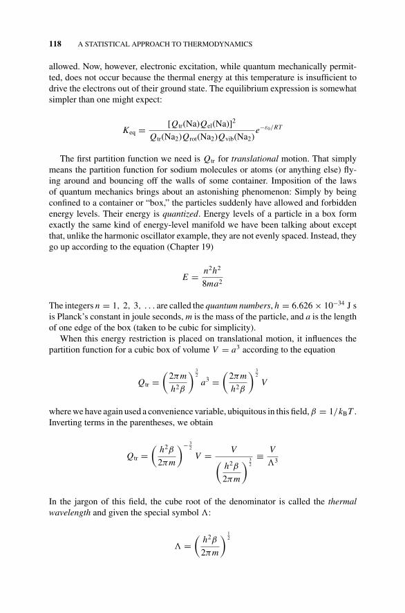
P1: OTA/XYZ P2: ABCc08 JWBS043-Rogers September 13, 2010 11:25 Printer Name: Yet to Come
118 A STATISTICAL APPROACH TO THERMODYNAMICS
allowed. Now, however, electronic excitation, while quantum mechanically permit-ted, does not occur because the thermal energy at this temperature is insufficient todrive the electrons out of their ground state. The equilibrium expression is somewhatsimpler than one might expect:
Keq = [Qtr(Na)Qel(Na)]2
Qtr(Na2)Qrot(Na2)Qvib(Na2)e−ε0/RT
The first partition function we need is Qtr for translational motion. That simplymeans the partition function for sodium molecules or atoms (or anything else) fly-ing around and bouncing off the walls of some container. Imposition of the lawsof quantum mechanics brings about an astonishing phenomenon: Simply by beingconfined to a container or “box,” the particles suddenly have allowed and forbiddenenergy levels. Their energy is quantized. Energy levels of a particle in a box formexactly the same kind of energy-level manifold we have been talking about exceptthat, unlike the harmonic oscillator example, they are not evenly spaced. Instead, theygo up according to the equation (Chapter 19)
E = n2h2
8ma2
The integers n = 1, 2, 3, . . . are called the quantum numbers, h = 6.626 × 10⁻³⁴ J sis Planck’s constant in joule seconds, m is the mass of the particle, and a is the lengthof one edge of the box (taken to be cubic for simplicity).
When this energy restriction is placed on translational motion, it influences thepartition function for a cubic box of volume V = a3 according to the equation
Qtr =(
2πm
h2β
) 32
a3 =(
2πm
h2β
) 32
V
where we have again used a convenience variable, ubiquitous in this field, β = 1/kBT .Inverting terms in the parentheses, we obtain
Qtr =(
h2β
2πm
)− 32
V = V(h2β
2πm
) 32
≡ V
3
In the jargon of this field, the cube root of the denominator is called the thermalwavelength and given the special symbol :
=(
h2β
2πm
) 12
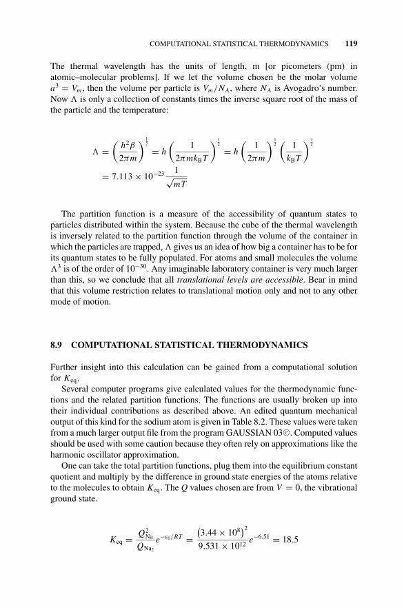
P1: OTA/XYZ P2: ABCc08 JWBS043-Rogers September 13, 2010 11:25 Printer Name: Yet to Come
COMPUTATIONAL STATISTICAL THERMODYNAMICS 119
The thermal wavelength has the units of length, m [or picometers (pm) inatomic–molecular problems]. If we let the volume chosen be the molar volumea3 = Vm , then the volume per particle is Vm/NA, where NA is Avogadro’s number.Now is only a collection of constants times the inverse square root of the mass ofthe particle and the temperature:
=(
h2β
2πm
) 12
= h
(1
2πmkBT
) 12
= h
(1
2πm
) 12(
1
kBT
) 12
= 7.113 × 10⁻²³ 1√mT
The partition function is a measure of the accessibility of quantum states toparticles distributed within the system. Because the cube of the thermal wavelengthis inversely related to the partition function through the volume of the container inwhich the particles are trapped, gives us an idea of how big a container has to be forits quantum states to be fully populated. For atoms and small molecules the volume3 is of the order of 10−30. Any imaginable laboratory container is very much largerthan this, so we conclude that all translational levels are accessible. Bear in mindthat this volume restriction relates to translational motion only and not to any othermode of motion.
8.9 COMPUTATIONAL STATISTICAL THERMODYNAMICS
Further insight into this calculation can be gained from a computational solutionfor Keq.
Several computer programs give calculated values for the thermodynamic func-tions and the related partition functions. The functions are usually broken up intotheir individual contributions as described above. An edited quantum mechanicaloutput of this kind for the sodium atom is given in Table 8.2. These values were takenfrom a much larger output file from the program GAUSSIAN 03 C©. Computed valuesshould be used with some caution because they often rely on approximations like theharmonic oscillator approximation.
One can take the total partition functions, plug them into the equilibrium constantquotient and multiply by the difference in ground state energies of the atoms relativeto the molecules to obtain Keq. The Q values chosen are from V = 0, the vibrationalground state.
Keq = Q2Na
QNa2
e−ε0/RT =(3.44 × 10⁸
)2
9.531 × 10¹²e−6.51 = 18.5
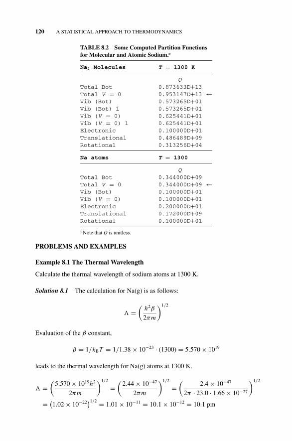
P1: OTA/XYZ P2: ABCc08 JWBS043-Rogers September 13, 2010 11:25 Printer Name: Yet to Come
120 A STATISTICAL APPROACH TO THERMODYNAMICS
TABLE 8.2 Some Computed Partition Functionsfor Molecular and Atomic Sodium.a
Na2 Molecules T = 1300 K
QTotal Bot 0.873633D+13Total V = 0 0.953147D+13 ←Vib (Bot) 0.573265D+01Vib (Bot) 1 0.573265D+01Vib (V = 0) 0.625441D+01Vib (V = 0) 1 0.625441D+01Electronic 0.100000D+01Translational 0.486489D+09Rotational 0.313256D+04Na atoms T = 1300
QTotal Bot 0.344000D+09Total V = 0 0.344000D+09 ←Vib (Bot) 0.100000D+01Vib (V = 0) 0.100000D+01Electronic 0.200000D+01Translational 0.172000D+09Rotational 0.100000D+01aNote that Q is unitless.
PROBLEMS AND EXAMPLES
Example 8.1 The Thermal Wavelength
Calculate the thermal wavelength of sodium atoms at 1300 K.
Solution 8.1 The calculation for Na(g) is as follows:
=(
h2β
2πm
)1/2
Evaluation of the β constant,
β = 1/kBT = 1/1.38 × 10−23 · (1300) = 5.570 × 10¹⁹
leads to the thermal wavelength for Na(g) atoms at 1300 K.
=(
5.570 × 10¹⁹h2
2πm
)1/2
=(
2.44 × 10−47
2πm
)1/2
=(
2.4 × 10−47
2π · 23.0 · 1.66 × 10−27
)1/2
= (1.02 × 10⁻²²)1/2 = 1.01 × 10−11 = 10.1 × 10−12 = 10.1 pm
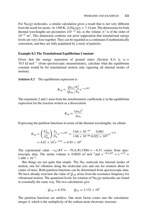
P1: OTA/XYZ P2: ABCc08 JWBS043-Rogers September 13, 2010 11:25 Printer Name: Yet to Come
PROBLEMS AND EXAMPLES 121
For Na2(g) molecules, a similar calculation gives a result that is not very differentfrom the result for atoms. At 1300 K, (Na2(g)) = 7.14 pm. The dimensions for boththermal wavelengths are picometers
(10−12 m
), so the volume 3 is of the order of
10−33 m3. This dimension confirms our prior supposition that translational energylevels are very close together. They can be regarded as a continuum if mathematicallyconvenient, and they are fully populated by a mole of particles.
Example 8.2 The Translational Equilibrium Constant
Given that the energy separation of ground states (Section 8.3) is ε0 =70.5 kJ mol−1 (from spectroscopic measurements), calculate what the equilibriumconstant would be for translational motion only (ignoring all internal modes ofmotion).
Solution 8.2 The equilibrium expression is
Keq = QNa/N 2A
QNa2/NAe−ε0/RT
The exponents 2 and 1 arise from the stoichiometric coefficients ξ in the equilibriumexpression for the reaction written as a dissociation
Keq = (pNa)2
pNa2
Expressing the partition functions in terms of the thermal wavelengths, we obtain
Keq =(
3Na2
6Na
)Vm
NAe−ε0/RT = 3.64 × 10⁻³⁴
1.06 × 10−66
0.082
6.022 × 10²³e−6.51
= 4.67 × 10⁷e−6.51 = 6.95 × 10⁴
The exponential value −ε0/RT = −70.4/R (1300) = −6.51 comes from spec-troscopic data. The molar volume is 0.0820 m3 mol−1and e−70.4/RT = e−6.51 =1.488 × 10⁻³.
But things are not quite that simple. The Na2 molecule has internal modes ofmotion, one for vibration along the molecular axis and one for rotation about itscenter of mass. Both partition functions can be determined from spectroscopic data.We have already seen how the value of Qvib arises from the resonance frequency forvibrational motion. The quantized levels for rotation of Na2(g) molecules are foundin essentially the same way. The two calculations give
Qvib = 6.254, Qrot = 3.132 × 10³
The partition functions are unitless. One more factor comes into the calculation:integer 4, which is the multiplicity of the sodium atom electronic structure.
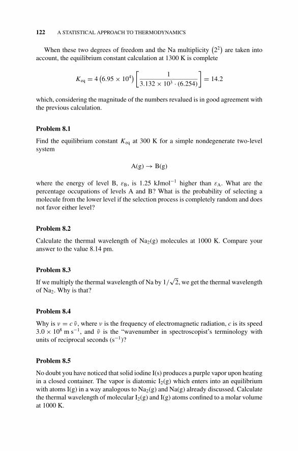
P1: OTA/XYZ P2: ABCc08 JWBS043-Rogers September 13, 2010 11:25 Printer Name: Yet to Come
122 A STATISTICAL APPROACH TO THERMODYNAMICS
When these two degrees of freedom and the Na multiplicity(22
)are taken into
account, the equilibrium constant calculation at 1300 K is complete
Keq = 4(6.95 × 10⁴
) [1
3.132 × 103 · (6.254)
]= 14.2
which, considering the magnitude of the numbers revalued is in good agreement withthe previous calculation.
Problem 8.1
Find the equilibrium constant Keq at 300 K for a simple nondegenerate two-levelsystem
A(g) → B(g)
where the energy of level B, εB, is 1.25 kJmol−1 higher than εA. What are thepercentage occupations of levels A and B? What is the probability of selecting amolecule from the lower level if the selection process is completely random and doesnot favor either level?
Problem 8.2
Calculate the thermal wavelength of Na2(g) molecules at 1000 K. Compare youranswer to the value 8.14 pm.
Problem 8.3
If we multiply the thermal wavelength of Na by 1/√
2, we get the thermal wavelengthof Na2. Why is that?
Problem 8.4
Why is ν = c ν, where ν is the frequency of electromagnetic radiation, c is its speed3.0 × 108 m s−1, and ν is the “wavenumber in spectroscopist’s terminology withunits of reciprocal seconds (s−1)?
Problem 8.5
No doubt you have noticed that solid iodine I(s) produces a purple vapor upon heatingin a closed container. The vapor is diatomic I2(g) which enters into an equilibriumwith atoms I(g) in a way analogous to Na2(g) and Na(g) already discussed. Calculatethe thermal wavelength of molecular I2(g) and I(g) atoms confined to a molar volumeat 1000 K.
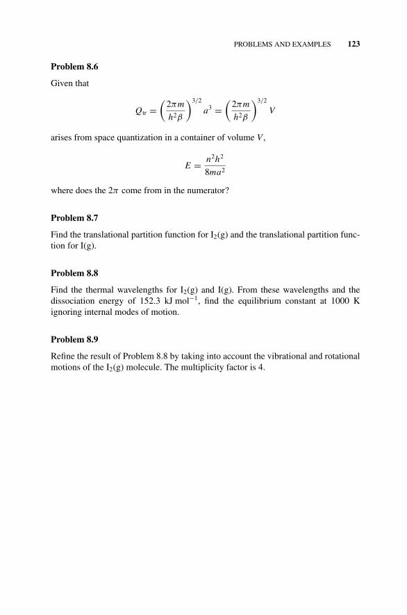
P1: OTA/XYZ P2: ABCc08 JWBS043-Rogers September 13, 2010 11:25 Printer Name: Yet to Come
PROBLEMS AND EXAMPLES 123
Problem 8.6
Given that
Qtr =(
2πm
h2β
)3/2
a3 =(
2πm
h2β
)3/2
V
arises from space quantization in a container of volume V ,
E = n2h2
8ma2
where does the 2π come from in the numerator?
Problem 8.7
Find the translational partition function for I2(g) and the translational partition func-tion for I(g).
Problem 8.8
Find the thermal wavelengths for I2(g) and I(g). From these wavelengths and thedissociation energy of 152.3 kJ mol−1, find the equilibrium constant at 1000 Kignoring internal modes of motion.
Problem 8.9
Refine the result of Problem 8.8 by taking into account the vibrational and rotationalmotions of the I2(g) molecule. The multiplicity factor is 4.

P1: OTA/XYZ P2: ABCc09 JWBS043-Rogers September 13, 2010 11:26 Printer Name: Yet to Come
9THE PHASE RULE
It is essential in science for experiments to be repeated, tested, and verified beforebeing accepted into the body of theory.1 To duplicate thermochemical experiments,one must be able to duplicate the thermochemical system, and to do that we must knowhow many of its infinite number of physical properties—mass m, energy, entropy, theheat capacities C p and CV , refractive indices, and so on—must be specified.
A fundamental truth that we usually take for granted is that there is a certainnumber of variables that completely describe any selected system. When we measuresome of them, we know all we can ever know about the system and we can, inprinciple, calculate all the variables we haven’t measured from those that we have.Which variables are they and how many of them are there? Must we know a substantialportion of the infinite number of possibilities in order to define a thermochemicalsystem? If that were true, science as we know it would hardly be possible because wecould never really verify (or contradict) an experimental result by replication. This isthe problem that was solved by J. Willard Gibbs.
9.1 COMPONENTS, PHASES, AND DEGREES OF FREEDOM
Gibbs distinguished between components C of a system, which are chemically dis-tinguishable, and the phases P of a system, which are physically distinct. Thus, the
1There are exceptions. The science of cosmology offers interesting contradictions because we would behard pressed to duplicate the creation of the universe.
Concise Physical Chemistry, by Donald W. RogersCopyright C© 2011 John Wiley & Sons, Inc.
124

P1: OTA/XYZ P2: ABCc09 JWBS043-Rogers September 13, 2010 11:26 Printer Name: Yet to Come
COEXISTENCE CURVES 125
system ice and water has one component, identifiable as H2O, and two phases, solidand liquid. With his famous phase rule (see below), Gibbs specified the numberof degrees of freedom of thermochemical systems. Degrees of freedom are like theindependent variables of a system of algebraic equations or the basis vectors of acomplete set. Once a limited number of them have been specified, the others are nolonger free to take on arbitrary values. They are linear combinations of the set that isalready known. For this reason it is the number of independent variables that we getfrom the phase rule, not their identity. We are free to choose which of the identifiablequantities shall be taken as independent variables, but only up to the number specifiedby the phase rule.
In the case of liquid water, one might argue that there are three components, H+,OH−, and H2O, or even four, including H3O+. We ignore these and similar formsbecause they are obviously related to each other and are not independent. In purewater, we know that [H+] = [OH−] because the only source of the ions is dissociation:
H2O → H+ + OH−
That makes it clear that if we measure either one but only one, we know the other.When we do this, we find
[H+] = 10−7; therefore we know that
[OH−] = 10−7and
we can write a dissociation equilibrium constant for pure water2:
Kw =[H+] [
OH−][H2O]
≈[H+]2
[H2O]=
[10−7
]2
1= 10−14
where the concentrations are expressed as moles per mole of solvent (water).Pursuing these ideas just a little further, what we call “concentrations” in solution
chemistry are really activities that, as unitless numbers (ratios relative to a standardstate), give a unitless Kw .
If we reformulate so as to include higher polymers such as H5O+2 , and so on,
their concentrations are not independent either because dissociation constants existby which we could calculate their concentration. These calculations are, in principle,possible, even though we may not have enough information to carry them out.However you look at it, specifying one molar concentration specifies them all. Thereis one component in a pure phase.
9.2 COEXISTENCE CURVES
The thermodynamic state of water vapor, H2O(g), like that of any pure substance, hastwo degrees of freedom. Any state function, including the Gibbs free energy, can beexpressed as a mathematical function of two independent variables, for example, µ =f (p, T ). We can also write E = f (p, T ) or C p = f (p, T ). In principle, equations
2By our conventional definition, pH ≡ − log[H+]
; this leads us to say that an aqueous solution is neutralwhen its pH = 7.
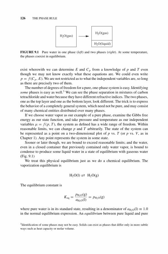
P1: OTA/XYZ P2: ABCc09 JWBS043-Rogers September 13, 2010 11:26 Printer Name: Yet to Come
126 THE PHASE RULE
H2O(gas)
H2O(liquid)
H2O(gas)
FIGURE 9.1 Pure water in one phase (left) and two phases (right). At some temperature,the phases coexist in equilibrium.
exist wherewith we can determine E and C p from a knowledge of p and T eventhough we may not know exactly what these equations are. We could even writep = f (C p, E). We are not restricted as to what the independent variables are, so longas there are precisely two of them.
The number of degrees of freedom for a pure, one-phase system is easy. Identifyingsome phases is easy as well.3 We can see the phase separation in mixtures of carbontetrachloride and water because they have different refractive indices. The two phases,one as the top layer and one as the bottom layer, look different. The trick is to expressthe behavior of a completely general system, which need not be pure, and may consistof many chemical entities distributed over many phases.
If we choose water vapor as our example of a pure phase, examine the Gibbs freeenergy as our state function, and take pressure and temperature as our independentvariables µ = f (p, T ), the system as defined has a wide range of freedom. Withinreasonable limits, we can change p and T arbitrarily. The state of the system canbe represented as a point on a two-dimensional plot of p vs. T (or p vs. V , as inChapter 1). Any point represents the system in some state.
Sooner or later though, we are bound to exceed reasonable limits; and the water,even in a closed container that previously contained only water vapor, is bound tocondense to produce some liquid water in a state of equilibrium with gaseous water(Fig. 9.1)
We treat this physical equilibrium just as we do a chemical equilibrium. Thevaporization equilibrium is
H2O(l) →← H2O(g)
The equilibrium constant is
Keq = pH2O(g)
aH2O(l)= pH2O(g)
where pure water is in its standard state, resulting in a denominator of aH2O(l) ≡ 1.0in the normal equilibrium expression. An equilibrium between pure liquid and pure
3Identification of some phases may not be easy. Solids can exist as phases that differ only in more subtleways such as heat capacity or molar volume.
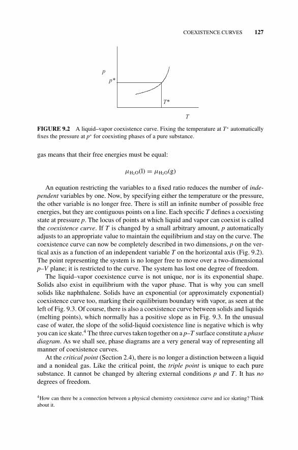
P1: OTA/XYZ P2: ABCc09 JWBS043-Rogers September 13, 2010 11:26 Printer Name: Yet to Come
COEXISTENCE CURVES 127
p
T
T*
p*
FIGURE 9.2 A liquid–vapor coexistence curve. Fixing the temperature at T* automaticallyfixes the pressure at p* for coexisting phases of a pure substance.
gas means that their free energies must be equal:
µH2O(l) = µH2O(g)
An equation restricting the variables to a fixed ratio reduces the number of inde-pendent variables by one. Now, by specifying either the temperature or the pressure,the other variable is no longer free. There is still an infinite number of possible freeenergies, but they are contiguous points on a line. Each specific T defines a coexistingstate at pressure p. The locus of points at which liquid and vapor can coexist is calledthe coexistence curve. If T is changed by a small arbitrary amount, p automaticallyadjusts to an appropriate value to maintain the equilibrium and stay on the curve. Thecoexistence curve can now be completely described in two dimensions, p on the ver-tical axis as a function of an independent variable T on the horizontal axis (Fig. 9.2).The point representing the system is no longer free to move over a two-dimensionalp–V plane; it is restricted to the curve. The system has lost one degree of freedom.
The liquid–vapor coexistence curve is not unique, nor is its exponential shape.Solids also exist in equilibrium with the vapor phase. That is why you can smellsolids like naphthalene. Solids have an exponential (or approximately exponential)coexistence curve too, marking their equilibrium boundary with vapor, as seen at theleft of Fig. 9.3. Of course, there is also a coexistence curve between solids and liquids(melting points), which normally has a positive slope as in Fig. 9.3. In the unusualcase of water, the slope of the solid-liquid coexistence line is negative which is whyyou can ice skate.4 The three curves taken together on a p–T surface constitute a phasediagram. As we shall see, phase diagrams are a very general way of representing allmanner of coexistence curves.
At the critical point (Section 2.4), there is no longer a distinction between a liquidand a nonideal gas. Like the critical point, the triple point is unique to each puresubstance. It cannot be changed by altering external conditions p and T . It has nodegrees of freedom.
4How can there be a connection between a physical chemistry coexistence curve and ice skating? Thinkabout it.
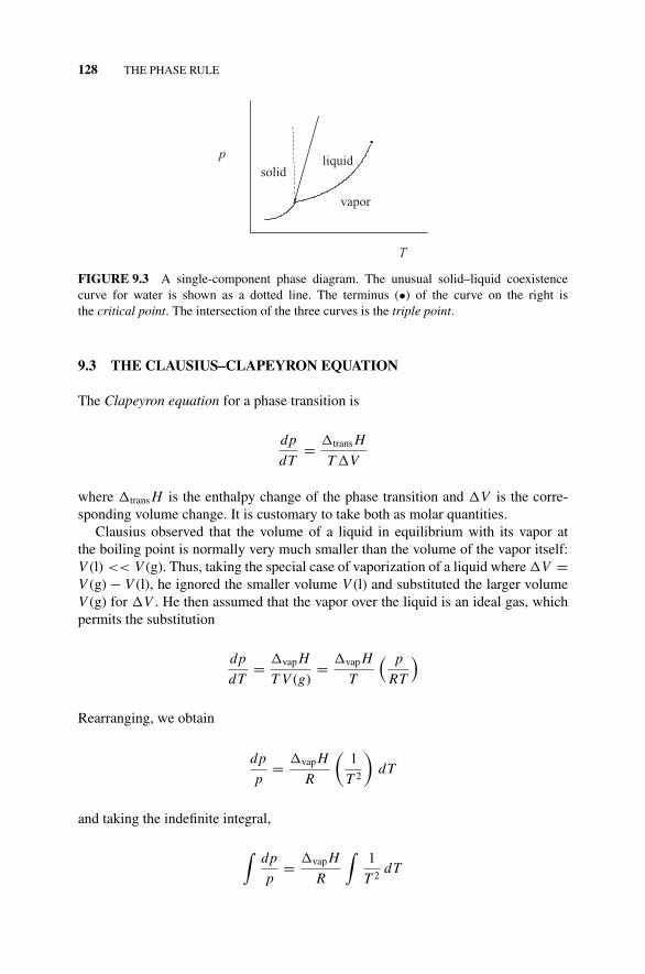
P1: OTA/XYZ P2: ABCc09 JWBS043-Rogers September 13, 2010 11:26 Printer Name: Yet to Come
128 THE PHASE RULE
p
T
.
vapor
liquidsolid
FIGURE 9.3 A single-component phase diagram. The unusual solid–liquid coexistencecurve for water is shown as a dotted line. The terminus (•) of the curve on the right isthe critical point. The intersection of the three curves is the triple point.
9.3 THE CLAUSIUS–CLAPEYRON EQUATION
The Clapeyron equation for a phase transition is
dp
dT= �trans H
T �V
where �trans H is the enthalpy change of the phase transition and �V is the corre-sponding volume change. It is customary to take both as molar quantities.
Clausius observed that the volume of a liquid in equilibrium with its vapor atthe boiling point is normally very much smaller than the volume of the vapor itself:V (l) << V (g). Thus, taking the special case of vaporization of a liquid where �V =V (g) − V (l), he ignored the smaller volume V (l) and substituted the larger volumeV (g) for �V . He then assumed that the vapor over the liquid is an ideal gas, whichpermits the substitution
dp
dT= �vap H
T V (g)= �vap H
T
( p
RT
)
Rearranging, we obtain
dp
p= �vap H
R
(1
T 2
)dT
and taking the indefinite integral,
∫dp
p= �vap H
R
∫1
T 2dT
P1: OTA/XYZ P2: ABCc09 JWBS043-Rogers September 13, 2010 11:26 Printer Name: Yet to Come
PARTIAL MOLAR VOLUME 129
we get
ln p = �vap H
R
(−1
T
)+ const.
This result can be written
pvap = ae−�vap H/RT = aeb(−1/T )
where a arises from the constant of integration. This is a form of theClausius–Clapeyron equation. If one can determine b in this exponential equation,then one has �vap H .
If an open container of liquid under an external pressure pext is heated to itsboiling point, bubbles form at the bottom of the container, each of which forms atiny closed “chamber” filled with pure vapor. That is why we observe that the normalboiling points of pure liquids observed in an open container follow the same equation(Clausius–Clapeyron) as that derived from the coexistence curve of the liquid in aclosed container.
9.4 PARTIAL MOLAR VOLUME
Prior to Gibbs, thermodynamics was largely about the transfer of heat in the processof driving an engine. It was an age justly called the age of steam. Gibbs’s departurewas to focus on the transfer of matter. That is why Gibbs’s work is so important tochemists. Our science is largely devoted to the transfer of matter from a reactant stateto a product state. In classical physical chemistry, we ask whether the transfer occurs(thermodynamics) and, if it does, we want to know how long it takes (kinetics).
To answer the first of these questions, Gibbs used partial molar thermodynamicstate functions. To start out, we shall consider the volume of a system and we shallrestrict mixtures to two components. The volume of a system is easy to visualize,and restricting the system to two components simplifies the arithmetic. Later we shallrelease these restrictions.
The volume of an ideal two-component liquid solution at constant p and T dependson how much of each component is present:
V = f (n1, n2)
If the molar volume of pure component 1 is V ◦m1 and the molar volume of pure
component 2 is V ◦m2, then an ideal solution of equal molar amounts of 1 and 2 will have
a molar volume that is the average of the two(V ◦
m1 + V ◦m2
)/2 (Fig. 9.4). Solutions of
other ratios of components 1 and 2 would be arrayed along a straight line connectingV ◦
m1 to V ◦m2, provided that no shrinkage or swelling takes place when 1 and 2 are mixed.
In general, for different ratios of the components, we obtain
V = V ◦m1n1 + V ◦
m2n2
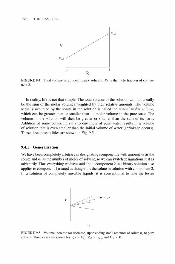
P1: OTA/XYZ P2: ABCc09 JWBS043-Rogers September 13, 2010 11:26 Printer Name: Yet to Come
130 THE PHASE RULE
0 1X2
Vm1
Vm2
V
FIGURE 9.4 Total volume of an ideal binary solution. X2 is the mole fraction of compo-nent 2.
In reality, life is not that simple. The total volume of the solution will not usuallybe the sum of the molar volumes weighted by their relative amounts. The volumeactually occupied by the solute in the solution is called the partial molar volume,which can be greater than or smaller than its molar volume in the pure state. Thevolume of the solution will then be greater or smaller than the sum of its parts.Addition of some potassium salts to one mole of pure water results in a volumeof solution that is even smaller than the initial volume of water (shrinkage occurs).These three possibilities are shown in Fig. 9.5.
9.4.1 Generalization
We have been completely arbitrary in designating component 2 with amount n2 as thesolute and n1 as the number of moles of solvent, so we can switch designations just asarbitrarily. Thus everything we have said about component 2 in a binary solution alsoapplies to component 1 treated as though it is the solute in solution with component 2.In a solution of completely miscible liquids, it is conventional to take the lesser
V
n2
V on2
FIGURE 9.5 Volume increase (or decrease) upon adding small amounts of solute n2 to puresolvent. Three cases are shown for Vn2 > V ◦
n2, Vn2 < V ◦n2, and Vn2 < 0.
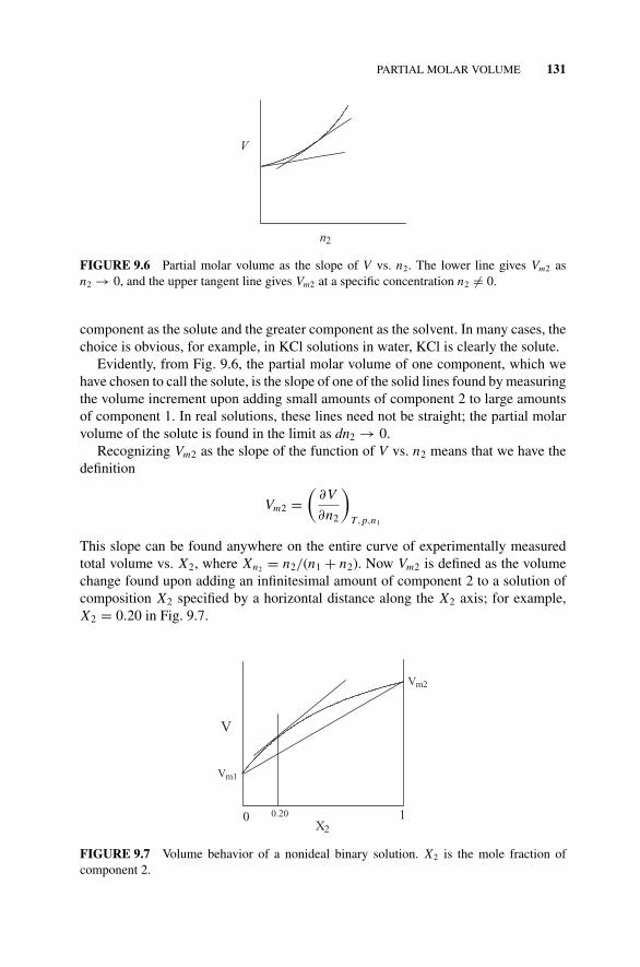
P1: OTA/XYZ P2: ABCc09 JWBS043-Rogers September 13, 2010 11:26 Printer Name: Yet to Come
PARTIAL MOLAR VOLUME 131
V
n2
FIGURE 9.6 Partial molar volume as the slope of V vs. n2. The lower line gives Vm2 asn2 → 0, and the upper tangent line gives Vm2 at a specific concentration n2 �= 0.
component as the solute and the greater component as the solvent. In many cases, thechoice is obvious, for example, in KCl solutions in water, KCl is clearly the solute.
Evidently, from Fig. 9.6, the partial molar volume of one component, which wehave chosen to call the solute, is the slope of one of the solid lines found by measuringthe volume increment upon adding small amounts of component 2 to large amountsof component 1. In real solutions, these lines need not be straight; the partial molarvolume of the solute is found in the limit as dn2 → 0.
Recognizing Vm2 as the slope of the function of V vs. n2 means that we have thedefinition
Vm2 =(
∂V
∂n2
)T,p,n1
This slope can be found anywhere on the entire curve of experimentally measuredtotal volume vs. X2, where Xn2 = n2/(n1 + n2). Now Vm2 is defined as the volumechange found upon adding an infinitesimal amount of component 2 to a solution ofcomposition X2 specified by a horizontal distance along the X2 axis; for example,X2 = 0.20 in Fig. 9.7.
0 1X2
Vm1
Vm2
V
0.20
FIGURE 9.7 Volume behavior of a nonideal binary solution. X2 is the mole fraction ofcomponent 2.
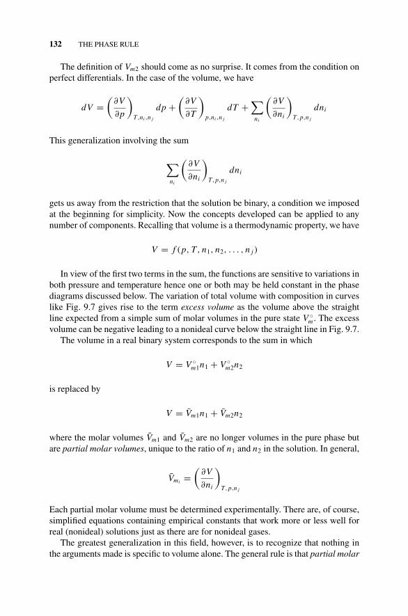
P1: OTA/XYZ P2: ABCc09 JWBS043-Rogers September 13, 2010 11:26 Printer Name: Yet to Come
132 THE PHASE RULE
The definition of Vm2 should come as no surprise. It comes from the condition onperfect differentials. In the case of the volume, we have
dV =(
∂V
∂p
)T,ni ,n j
dp +(
∂V
∂T
)p,ni ,n j
dT +∑
ni
(∂V
∂ni
)T,p,n j
dni
This generalization involving the sum
∑ni
(∂V
∂ni
)T,p,n j
dni
gets us away from the restriction that the solution be binary, a condition we imposedat the beginning for simplicity. Now the concepts developed can be applied to anynumber of components. Recalling that volume is a thermodynamic property, we have
V = f (p, T, n1, n2, . . . , n j )
In view of the first two terms in the sum, the functions are sensitive to variations inboth pressure and temperature hence one or both may be held constant in the phasediagrams discussed below. The variation of total volume with composition in curveslike Fig. 9.7 gives rise to the term excess volume as the volume above the straightline expected from a simple sum of molar volumes in the pure state V ◦
m . The excessvolume can be negative leading to a nonideal curve below the straight line in Fig. 9.7.
The volume in a real binary system corresponds to the sum in which
V = V ◦m1n1 + V ◦
m2n2
is replaced by
V = Vm1n1 + Vm2n2
where the molar volumes Vm1 and Vm2 are no longer volumes in the pure phase butare partial molar volumes, unique to the ratio of n1 and n2 in the solution. In general,
Vmi =(
∂V
∂ni
)T,p,n j
Each partial molar volume must be determined experimentally. There are, of course,simplified equations containing empirical constants that work more or less well forreal (nonideal) solutions just as there are for nonideal gases.
The greatest generalization in this field, however, is to recognize that nothing inthe arguments made is specific to volume alone. The general rule is that partial molar

P1: OTA/XYZ P2: ABCc09 JWBS043-Rogers September 13, 2010 11:26 Printer Name: Yet to Come
PARTIAL MOLAR VOLUME 133
quantities analogous to the partial molar volume exist for all thermodynamic statevariables. This rule gives us the partial molar energy,
Umi =(
∂U
∂ni
)T,p,n j
the partial molar enthalpy,
Hmi =(
∂ H
∂ni
)T,p,n j
the partial molar entropy,
Smi =(
∂S
∂ni
)T,p,n j
and the partial molar Gibbs free energy
µmi =(
∂µ
∂ni
)T,p,n j
This last partial molar quantity is so important that it is given a unique name andsymbol. It is called the Gibbs chemical potential µmi . It should be clear that in real(nonideal) systems, each of these functions has a corresponding excess function; theexcess energy, the excess enthalpy, the excess entropy, and so on.
In generalizing thermodynamics to many-component systems, Gibbs broughtabout an immense expansion of the scope of the subject. All of the classical ther-modynamic equations apply to partial molar quantities as well. For example, byanalogy to
d
(G
T
)
d
(1
T
) = H
for the Gibbs free energy of ideal components (Section 6.6), we have
d(µ
T
)
d
(1
T
) = H m
relating the partial molar Gibbs free energy and the partial molar enthalpy. H m .
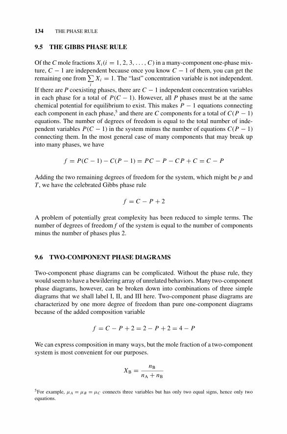
P1: OTA/XYZ P2: ABCc09 JWBS043-Rogers September 13, 2010 11:26 Printer Name: Yet to Come
134 THE PHASE RULE
9.5 THE GIBBS PHASE RULE
Of the C mole fractions Xi (i = 1, 2, 3, . . . , C) in a many-component one-phase mix-ture, C − 1 are independent because once you know C − 1 of them, you can get theremaining one from
∑i
Xi = 1. The “last” concentration variable is not independent.
If there are P coexisting phases, there are C − 1 independent concentration variablesin each phase for a total of P(C − 1). However, all P phases must be at the samechemical potential for equilibrium to exist. This makes P − 1 equations connectingeach component in each phase,5 and there are C components for a total of C(P − 1)equations. The number of degrees of freedom is equal to the total number of inde-pendent variables P(C − 1) in the system minus the number of equations C(P − 1)connecting them. In the most general case of many components that may break upinto many phases, we have
f = P(C − 1) − C(P − 1) = PC − P − C P + C = C − P
Adding the two remaining degrees of freedom for the system, which might be p andT , we have the celebrated Gibbs phase rule
f = C − P + 2
A problem of potentially great complexity has been reduced to simple terms. Thenumber of degrees of freedom f of the system is equal to the number of componentsminus the number of phases plus 2.
9.6 TWO-COMPONENT PHASE DIAGRAMS
Two-component phase diagrams can be complicated. Without the phase rule, theywould seem to have a bewildering array of unrelated behaviors. Many two-componentphase diagrams, however, can be broken down into combinations of three simplediagrams that we shall label I, II, and III here. Two-component phase diagrams arecharacterized by one more degree of freedom than pure one-component diagramsbecause of the added composition variable
f = C − P + 2 = 2 − P + 2 = 4 − P
We can express composition in many ways, but the mole fraction of a two-componentsystem is most convenient for our purposes.
XB = nB
nA + nB
5For example, µA = µB = µC connects three variables but has only two equal signs, hence only twoequations.
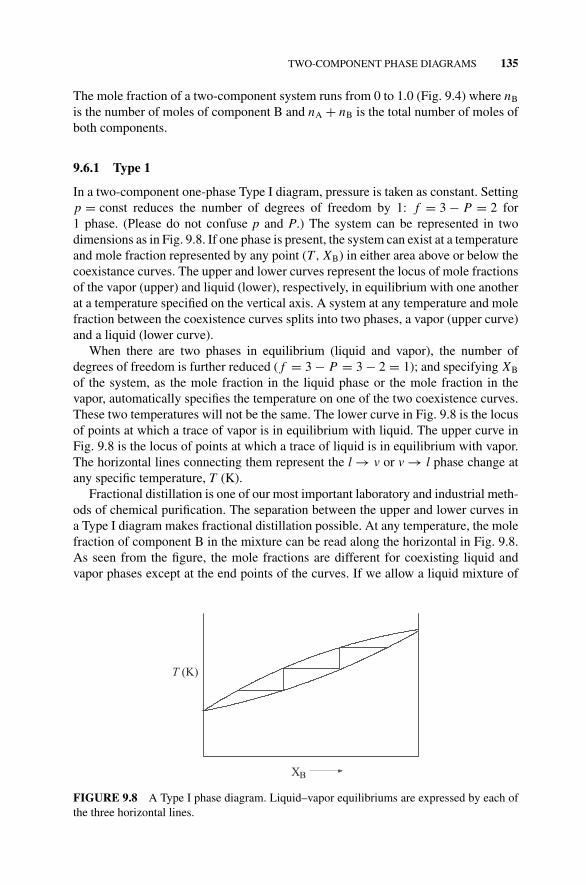
P1: OTA/XYZ P2: ABCc09 JWBS043-Rogers September 13, 2010 11:26 Printer Name: Yet to Come
TWO-COMPONENT PHASE DIAGRAMS 135
The mole fraction of a two-component system runs from 0 to 1.0 (Fig. 9.4) where nB
is the number of moles of component B and nA + nB is the total number of moles ofboth components.
9.6.1 Type 1
In a two-component one-phase Type I diagram, pressure is taken as constant. Settingp = const reduces the number of degrees of freedom by 1: f = 3 − P = 2 for1 phase. (Please do not confuse p and P.) The system can be represented in twodimensions as in Fig. 9.8. If one phase is present, the system can exist at a temperatureand mole fraction represented by any point (T, XB) in either area above or below thecoexistance curves. The upper and lower curves represent the locus of mole fractionsof the vapor (upper) and liquid (lower), respectively, in equilibrium with one anotherat a temperature specified on the vertical axis. A system at any temperature and molefraction between the coexistence curves splits into two phases, a vapor (upper curve)and a liquid (lower curve).
When there are two phases in equilibrium (liquid and vapor), the number ofdegrees of freedom is further reduced ( f = 3 − P = 3 − 2 = 1); and specifying XB
of the system, as the mole fraction in the liquid phase or the mole fraction in thevapor, automatically specifies the temperature on one of the two coexistence curves.These two temperatures will not be the same. The lower curve in Fig. 9.8 is the locusof points at which a trace of vapor is in equilibrium with liquid. The upper curve inFig. 9.8 is the locus of points at which a trace of liquid is in equilibrium with vapor.The horizontal lines connecting them represent the l → v or v → l phase change atany specific temperature, T (K).
Fractional distillation is one of our most important laboratory and industrial meth-ods of chemical purification. The separation between the upper and lower curves ina Type I diagram makes fractional distillation possible. At any temperature, the molefraction of component B in the mixture can be read along the horizontal in Fig. 9.8.As seen from the figure, the mole fractions are different for coexisting liquid andvapor phases except at the end points of the curves. If we allow a liquid mixture of
XB
T (K)
FIGURE 9.8 A Type I phase diagram. Liquid–vapor equilibriums are expressed by each ofthe three horizontal lines.
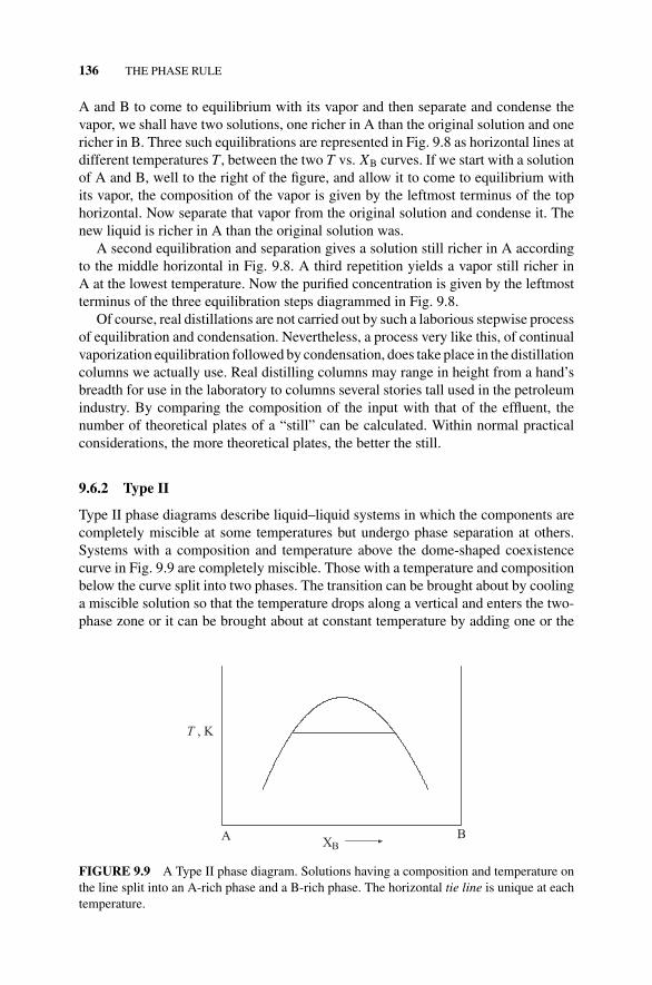
P1: OTA/XYZ P2: ABCc09 JWBS043-Rogers September 13, 2010 11:26 Printer Name: Yet to Come
136 THE PHASE RULE
A and B to come to equilibrium with its vapor and then separate and condense thevapor, we shall have two solutions, one richer in A than the original solution and onericher in B. Three such equilibrations are represented in Fig. 9.8 as horizontal lines atdifferent temperatures T , between the two T vs. XB curves. If we start with a solutionof A and B, well to the right of the figure, and allow it to come to equilibrium withits vapor, the composition of the vapor is given by the leftmost terminus of the tophorizontal. Now separate that vapor from the original solution and condense it. Thenew liquid is richer in A than the original solution was.
A second equilibration and separation gives a solution still richer in A accordingto the middle horizontal in Fig. 9.8. A third repetition yields a vapor still richer inA at the lowest temperature. Now the purified concentration is given by the leftmostterminus of the three equilibration steps diagrammed in Fig. 9.8.
Of course, real distillations are not carried out by such a laborious stepwise processof equilibration and condensation. Nevertheless, a process very like this, of continualvaporization equilibration followed by condensation, does take place in the distillationcolumns we actually use. Real distilling columns may range in height from a hand’sbreadth for use in the laboratory to columns several stories tall used in the petroleumindustry. By comparing the composition of the input with that of the effluent, thenumber of theoretical plates of a “still” can be calculated. Within normal practicalconsiderations, the more theoretical plates, the better the still.
9.6.2 Type II
Type II phase diagrams describe liquid–liquid systems in which the components arecompletely miscible at some temperatures but undergo phase separation at others.Systems with a composition and temperature above the dome-shaped coexistencecurve in Fig. 9.9 are completely miscible. Those with a temperature and compositionbelow the curve split into two phases. The transition can be brought about by coolinga miscible solution so that the temperature drops along a vertical and enters the two-phase zone or it can be brought about at constant temperature by adding one or the
XB
T , K
A B
FIGURE 9.9 A Type II phase diagram. Solutions having a composition and temperature onthe line split into an A-rich phase and a B-rich phase. The horizontal tie line is unique at eachtemperature.
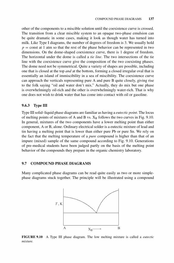
P1: OTA/XYZ P2: ABCc09 JWBS043-Rogers September 13, 2010 11:26 Printer Name: Yet to Come
COMPOUND PHASE DIAGRAMS 137
other of the components to a miscible solution until the coexistence curve is crossed.The transition from a clear miscible system to an opaque two-phase emulsion canbe quite dramatic in some cases, making it look as though water has turned intomilk. Like Type I diagrams, the number of degrees of freedom is 3. We usually holdp = const at 1 atm so that the rest of the phase behavior can be represented in twodimensions. On the dome-shaped coexistence curve, there is 1 degree of freedom.The horizontal under the dome is called a tie line. The two intersections of the tieline with the coexistence curve give the composition of the two coexisting phases.The dome need not be symmetrical. Quite a variety of shapes are possible, includingone that is closed at the top and at the bottom, forming a closed irregular oval that isessentially an island of immiscibility in a sea of miscibility. The coexistence curvecan approach the verticals representing pure A and pure B quite closely, giving riseto the folk saying “oil and water don’t mix.” Actually, they do mix but one phaseis overwhelmingly oil-rich and the other is overwhelmingly water-rich. That is whyone does not wish to drink water that has come into contact with oil or gasoline.
9.6.3 Type III
Type III solid–liquid phase diagrams are familiar as having a eutectic point. The locusof melting points of mixtures of A and B vs. XB follows the two curves in Fig. 9.10.In general, mixtures of the two components have a lower melting point than eithercomponent, A or B, alone. Ordinary electrical solder is a eutectic mixture of lead andtin having a melting point that is lower than either pure Pb or pure Sn. We rely onthe fact that the melting temperature of a pure compound is higher than that of animpure (mixed) sample of the same compound according to Fig. 9.10. Generationsof pre-medical students have been judged partly on the basis of the melting pointbehavior of the compounds they prepare in the organic chemistry laboratory.
9.7 COMPOUND PHASE DIAGRAMS
Many complicated phase diagrams can be read quite easily as two or more simple-phase diagrams stuck together. The principle will be illustrated using a compound
XB
T , K
A B
FIGURE 9.10 A Type III phase diagram. The low melting mixture is called a eutecticmixture.
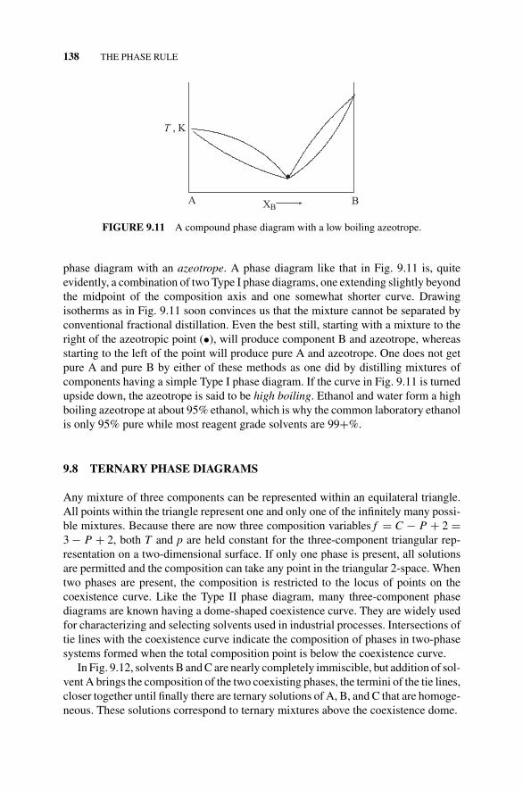
P1: OTA/XYZ P2: ABCc09 JWBS043-Rogers September 13, 2010 11:26 Printer Name: Yet to Come
138 THE PHASE RULE
XB
T , K
A B
.
FIGURE 9.11 A compound phase diagram with a low boiling azeotrope.
phase diagram with an azeotrope. A phase diagram like that in Fig. 9.11 is, quiteevidently, a combination of two Type I phase diagrams, one extending slightly beyondthe midpoint of the composition axis and one somewhat shorter curve. Drawingisotherms as in Fig. 9.11 soon convinces us that the mixture cannot be separated byconventional fractional distillation. Even the best still, starting with a mixture to theright of the azeotropic point (•), will produce component B and azeotrope, whereasstarting to the left of the point will produce pure A and azeotrope. One does not getpure A and pure B by either of these methods as one did by distilling mixtures ofcomponents having a simple Type I phase diagram. If the curve in Fig. 9.11 is turnedupside down, the azeotrope is said to be high boiling. Ethanol and water form a highboiling azeotrope at about 95% ethanol, which is why the common laboratory ethanolis only 95% pure while most reagent grade solvents are 99+%.
9.8 TERNARY PHASE DIAGRAMS
Any mixture of three components can be represented within an equilateral triangle.All points within the triangle represent one and only one of the infinitely many possi-ble mixtures. Because there are now three composition variables f = C − P + 2 =3 − P + 2, both T and p are held constant for the three-component triangular rep-resentation on a two-dimensional surface. If only one phase is present, all solutionsare permitted and the composition can take any point in the triangular 2-space. Whentwo phases are present, the composition is restricted to the locus of points on thecoexistence curve. Like the Type II phase diagram, many three-component phasediagrams are known having a dome-shaped coexistence curve. They are widely usedfor characterizing and selecting solvents used in industrial processes. Intersections oftie lines with the coexistence curve indicate the composition of phases in two-phasesystems formed when the total composition point is below the coexistence curve.
In Fig. 9.12, solvents B and C are nearly completely immiscible, but addition of sol-vent A brings the composition of the two coexisting phases, the termini of the tie lines,closer together until finally there are ternary solutions of A, B, and C that are homoge-neous. These solutions correspond to ternary mixtures above the coexistence dome.
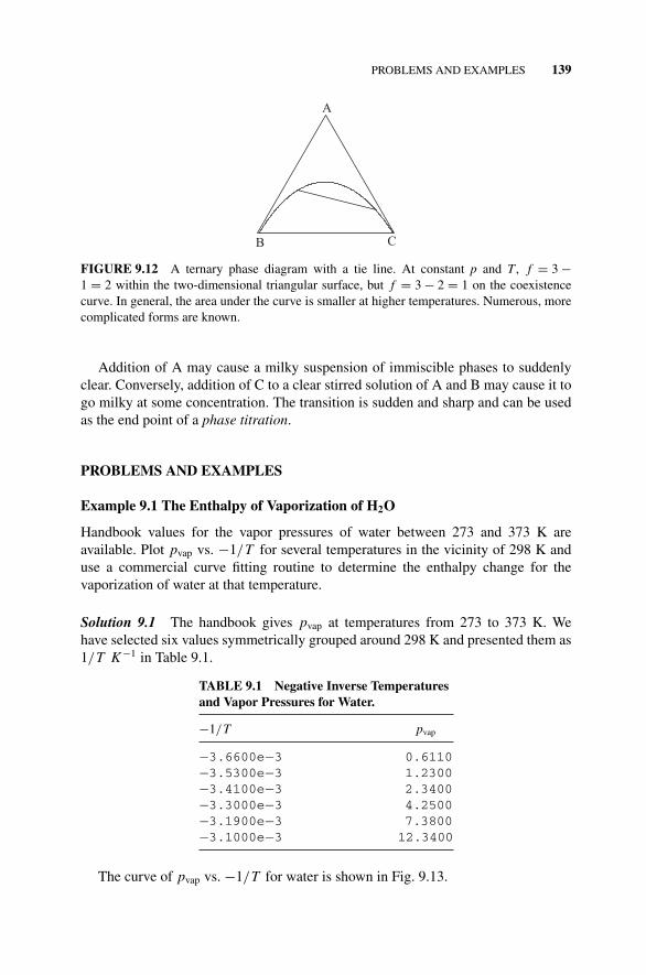
P1: OTA/XYZ P2: ABCc09 JWBS043-Rogers September 13, 2010 11:26 Printer Name: Yet to Come
PROBLEMS AND EXAMPLES 139
A
B C
FIGURE 9.12 A ternary phase diagram with a tie line. At constant p and T , f = 3 −1 = 2 within the two-dimensional triangular surface, but f = 3 − 2 = 1 on the coexistencecurve. In general, the area under the curve is smaller at higher temperatures. Numerous, morecomplicated forms are known.
Addition of A may cause a milky suspension of immiscible phases to suddenlyclear. Conversely, addition of C to a clear stirred solution of A and B may cause it togo milky at some concentration. The transition is sudden and sharp and can be usedas the end point of a phase titration.
PROBLEMS AND EXAMPLES
Example 9.1 The Enthalpy of Vaporization of H2O
Handbook values for the vapor pressures of water between 273 and 373 K areavailable. Plot pvap vs. −1/T for several temperatures in the vicinity of 298 K anduse a commercial curve fitting routine to determine the enthalpy change for thevaporization of water at that temperature.
Solution 9.1 The handbook gives pvap at temperatures from 273 to 373 K. Wehave selected six values symmetrically grouped around 298 K and presented them as1/T K −1 in Table 9.1.
TABLE 9.1 Negative Inverse Temperaturesand Vapor Pressures for Water.
−1/T pvap
−3.6600e−3 0.6110−3.5300e−3 1.2300−3.4100e−3 2.3400−3.3000e−3 4.2500−3.1900e−3 7.3800−3.1000e−3 12.3400
The curve of pvap vs. −1/T for water is shown in Fig. 9.13.
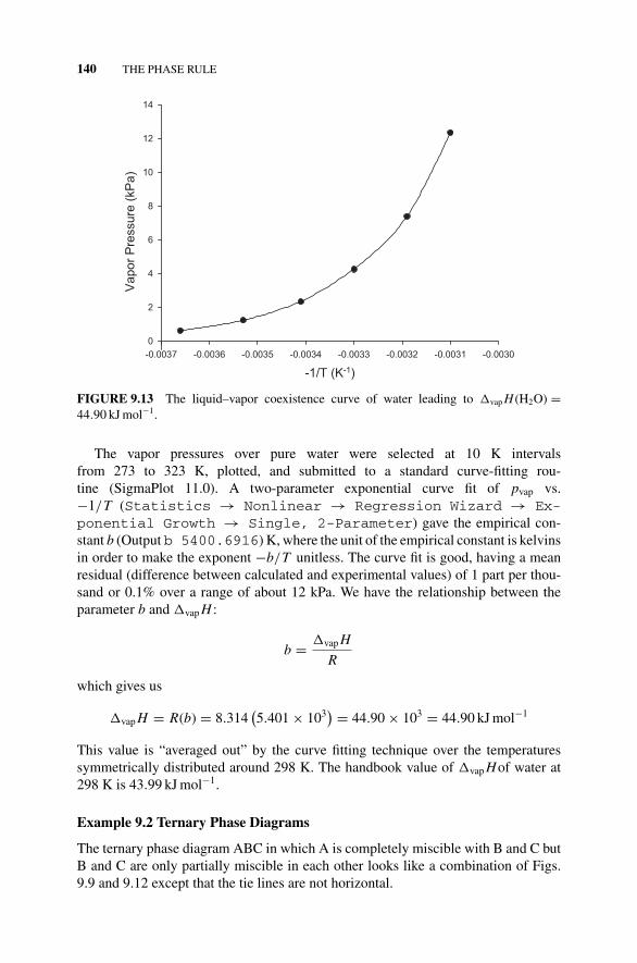
P1: OTA/XYZ P2: ABCc09 JWBS043-Rogers September 13, 2010 11:26 Printer Name: Yet to Come
140 THE PHASE RULE
-1/T (K-1)
-0.0037 -0.0036 -0.0035 -0.0034 -0.0033 -0.0032 -0.0031 -0.0030
Vapor
Pre
ssure
(kP
a)
0
2
4
6
8
10
12
14
FIGURE 9.13 The liquid–vapor coexistence curve of water leading to �vap H (H2O) =44.90 kJ mol−1.
The vapor pressures over pure water were selected at 10 K intervalsfrom 273 to 323 K, plotted, and submitted to a standard curve-fitting rou-tine (SigmaPlot 11.0). A two-parameter exponential curve fit of pvap vs.−1/T (Statistics → Nonlinear → Regression Wizard → Ex-ponential Growth → Single, 2-Parameter) gave the empirical con-stant b (Outputb 5400.6916) K, where the unit of the empirical constant is kelvinsin order to make the exponent −b/T unitless. The curve fit is good, having a meanresidual (difference between calculated and experimental values) of 1 part per thou-sand or 0.1% over a range of about 12 kPa. We have the relationship between theparameter b and �vap H :
b = �vap H
R
which gives us
�vap H = R(b) = 8.314(5.401 × 10³
) = 44.90 × 103 = 44.90 kJ mol−1
This value is “averaged out” by the curve fitting technique over the temperaturessymmetrically distributed around 298 K. The handbook value of �vap Hof water at298 K is 43.99 kJ mol−1.
Example 9.2 Ternary Phase Diagrams
The ternary phase diagram ABC in which A is completely miscible with B and C butB and C are only partially miscible in each other looks like a combination of Figs.9.9 and 9.12 except that the tie lines are not horizontal.
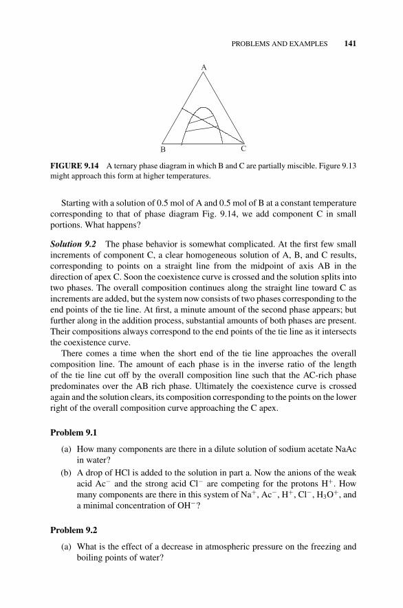
P1: OTA/XYZ P2: ABCc09 JWBS043-Rogers September 13, 2010 11:26 Printer Name: Yet to Come
PROBLEMS AND EXAMPLES 141
A
B C
FIGURE 9.14 A ternary phase diagram in which B and C are partially miscible. Figure 9.13might approach this form at higher temperatures.
Starting with a solution of 0.5 mol of A and 0.5 mol of B at a constant temperaturecorresponding to that of phase diagram Fig. 9.14, we add component C in smallportions. What happens?
Solution 9.2 The phase behavior is somewhat complicated. At the first few smallincrements of component C, a clear homogeneous solution of A, B, and C results,corresponding to points on a straight line from the midpoint of axis AB in thedirection of apex C. Soon the coexistence curve is crossed and the solution splits intotwo phases. The overall composition continues along the straight line toward C asincrements are added, but the system now consists of two phases corresponding to theend points of the tie line. At first, a minute amount of the second phase appears; butfurther along in the addition process, substantial amounts of both phases are present.Their compositions always correspond to the end points of the tie line as it intersectsthe coexistence curve.
There comes a time when the short end of the tie line approaches the overallcomposition line. The amount of each phase is in the inverse ratio of the lengthof the tie line cut off by the overall composition line such that the AC-rich phasepredominates over the AB rich phase. Ultimately the coexistence curve is crossedagain and the solution clears, its composition corresponding to the points on the lowerright of the overall composition curve approaching the C apex.
Problem 9.1
(a) How many components are there in a dilute solution of sodium acetate NaAcin water?
(b) A drop of HCl is added to the solution in part a. Now the anions of the weakacid Ac− and the strong acid Cl− are competing for the protons H+. Howmany components are there in this system of Na+, Ac−, H+, Cl−, H3O+, anda minimal concentration of OH−?
Problem 9.2
(a) What is the effect of a decrease in atmospheric pressure on the freezing andboiling points of water?
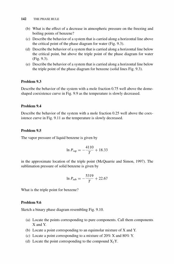
P1: OTA/XYZ P2: ABCc09 JWBS043-Rogers September 13, 2010 11:26 Printer Name: Yet to Come
142 THE PHASE RULE
(b) What is the effect of a decrease in atmospheric pressure on the freezing andboiling points of benzene?
(c) Describe the behavior of a system that is carried along a horizontal line abovethe critical point of the phase diagram for water (Fig. 9.3).
(d) Describe the behavior of a system that is carried along a horizontal line belowthe critical point, but above the triple point of the phase diagram for water(Fig. 9.3).
(e) Describe the behavior of a system that is carried along a horizontal line belowthe triple point of the phase diagram for benzene (solid lines Fig. 9.3).
Problem 9.3
Describe the behavior of the system with a mole fraction 0.75 well above the dome-shaped coexistence curve in Fig. 9.9 as the temperature is slowly decreased.
Problem 9.4
Describe the behavior of the system with a mole fraction 0.25 well above the coex-istence curve in Fig. 9.11 as the temperature is slowly decreased.
Problem 9.5
The vapor pressure of liquid benzene is given by
ln Pvap = −4110
T+ 18.33
in the approximate location of the triple point (McQuarrie and Simon, 1997). Thesublimation pressure of solid benzene is given by
ln Psub = −5319
T+ 22.67
What is the triple point for benzene?
Problem 9.6
Sketch a binary phase diagram resembling Fig. 9.10.
(a) Locate the points corresponding to pure components. Call them componentsX and Y.
(b) Locate a point corresponding to an equimolar mixture of X and Y.
(c) Locate a point corresponding to a mixture of 20% X and 80% Y.
(d) Locate the point corresponding to the compound X2Y.
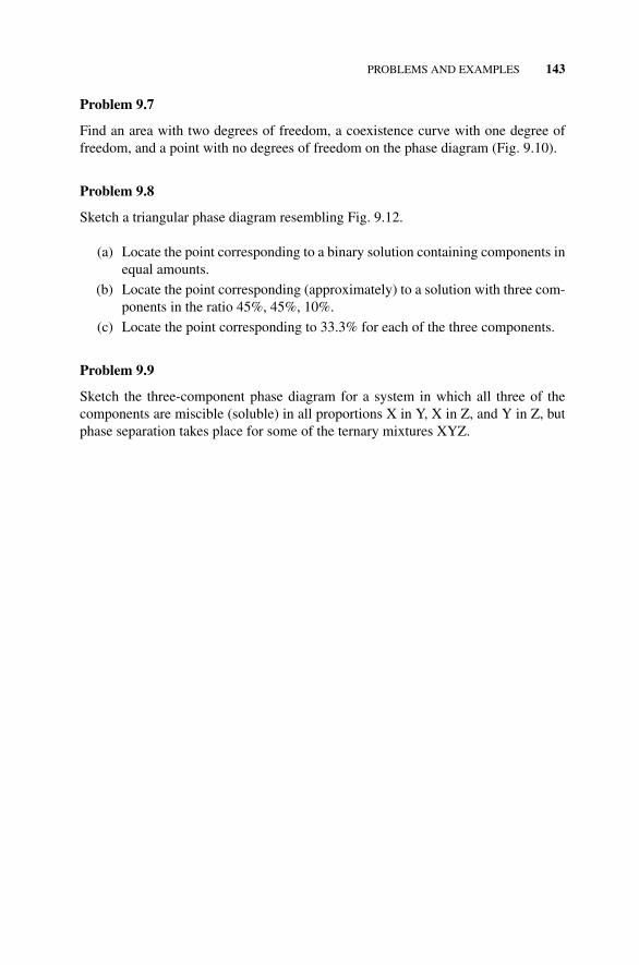
P1: OTA/XYZ P2: ABCc09 JWBS043-Rogers September 13, 2010 11:26 Printer Name: Yet to Come
PROBLEMS AND EXAMPLES 143
Problem 9.7
Find an area with two degrees of freedom, a coexistence curve with one degree offreedom, and a point with no degrees of freedom on the phase diagram (Fig. 9.10).
Problem 9.8
Sketch a triangular phase diagram resembling Fig. 9.12.
(a) Locate the point corresponding to a binary solution containing components inequal amounts.
(b) Locate the point corresponding (approximately) to a solution with three com-ponents in the ratio 45%, 45%, 10%.
(c) Locate the point corresponding to 33.3% for each of the three components.
Problem 9.9
Sketch the three-component phase diagram for a system in which all three of thecomponents are miscible (soluble) in all proportions X in Y, X in Z, and Y in Z, butphase separation takes place for some of the ternary mixtures XYZ.
P1: OTA/XYZ P2: ABCc10 JWBS043-Rogers September 13, 2010 11:26 Printer Name: Yet to Come
10CHEMICAL KINETICS
In general, chemical thermodynamics is concerned with where a chemical systemstarts and where it ends up, while chemical kinetics is concerned with how longit takes it to get there. Many analytical techniques exist for following the rate ofchange of the concentration of the reactants or products of a chemical reaction, butsingle atom counting is not usually done. An exception is the class of radiochemicalreactions for which counters exist to register, count, and record in computer memoryevery decay particle produced. For example, the decay of radium gives α particles(helium nuclei) and radon 222
86Rn:
22688Ra → 222
86Rn + 42He
Each click of the counter registers one α particle, hence one decay. Here radium isthe radioactive element, and both radon and helium are products. Radon is referred toas the daughter of the parent element radium. Radon is itself a radioactive gas, and itdecays to polonium and further along a radioactive series ending eventually as lead20682Pb. Radiochemical reactions show the statistical nature of rate laws very clearly,
For that reason, they are a good introduction to the entire field.
10.1 FIRST-ORDER KINETIC RATE LAWS
Suppose you have a sample consisting of a hundred billion atoms of radioactiveelement X. By means of a suitable counter, you observe an average of one radioactive
Concise Physical Chemistry, by Donald W. RogersCopyright C© 2011 John Wiley & Sons, Inc.
144
P1: OTA/XYZ P2: ABCc10 JWBS043-Rogers September 13, 2010 11:26 Printer Name: Yet to Come
FIRST-ORDER KINETIC RATE LAWS 145
decay per second. You have observed a rate of decay −d X/dt in the units (numberof atoms)/time, usually given as a frequency (s−1). Decay causes a decrease in thenumber of atoms X, which accounts for the minus sign in front of the rate. If youtake 200 billion atoms, you find twice as many radioactive events. That only standsto reason. Radioactive decay is a random phenomenon. Observing twice as manyatoms, one expects to see twice as many events in a specified time interval. Taking ktimes as many atoms gives k times as many radioactive events: rate = kX. Now youhave a rate, a rate law, and a rate equation. The rate of disintegration is
−dX
dt= kX
The rate of product production is equal but opposite in sign to the rate of decay.Provided that the daughter is not radioactive, starting with a number of atoms X0 at
a time t = t0 = 0 (an arbitrary time that you choose to start watching your counter),the average count rate gradually decreases with time. If you watch long enough,1 thecount rate will be reduced to half of what it was at t0. This is called the half-time ofthe radioactive element.
The rate equation can be rearranged to give
dX
X= −k dt
The ratio dX/X being unitless, −k dt must be unitless as well, so the unit of k is s−1
because t is in seconds. Integration between t0 and t is straightforward:
∫ t
t0
1
Xd X = −k
∫ t
t0
dt
gives
lnX
X0= −k(t − t0)
In exponential form
X
X0= e−k(t−t0)
X0 is the initial concentration (a constant) and t0 is usually set to zero so thatX0 = X (0) and
X = X0e−kt
1About 1600 years in the case of radium.
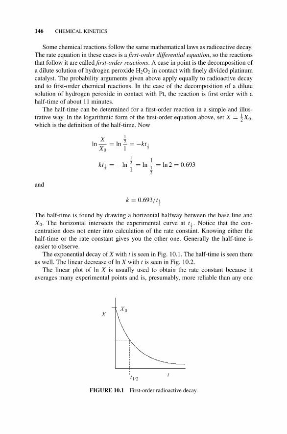
P1: OTA/XYZ P2: ABCc10 JWBS043-Rogers September 13, 2010 11:26 Printer Name: Yet to Come
146 CHEMICAL KINETICS
Some chemical reactions follow the same mathematical laws as radioactive decay.The rate equation in these cases is a first-order differential equation, so the reactionsthat follow it are called first-order reactions. A case in point is the decomposition ofa dilute solution of hydrogen peroxide H2O2 in contact with finely divided platinumcatalyst. The probability arguments given above apply equally to radioactive decayand to first-order chemical reactions. In the case of the decomposition of a dilutesolution of hydrogen peroxide in contact with Pt, the reaction is first order with ahalf-time of about 11 minutes.
The half-time can be determined for a first-order reaction in a simple and illus-trative way. In the logarithmic form of the first-order equation above, set X = 1
2 X0,which is the definition of the half-time. Now
lnX
X0= ln
12
1= −kt 1
2
kt 12
= − ln12
1= ln
112
= ln 2 = 0.693
and
k = 0.693/t 12
The half-time is found by drawing a horizontal halfway between the base line andX0. The horizontal intersects the experimental curve at t 1
2. Notice that the con-
centration does not enter into calculation of the rate constant. Knowing either thehalf-time or the rate constant gives you the other one. Generally the half-time iseasier to observe.
The exponential decay of X with t is seen in Fig. 10.1. The half-time is seen thereas well. The linear decrease of ln X with t is seen in Fig. 10.2.
The linear plot of ln X is usually used to obtain the rate constant because itaverages many experimental points and is, presumably, more reliable than any one
XX 0
tt1/2
FIGURE 10.1 First-order radioactive decay.
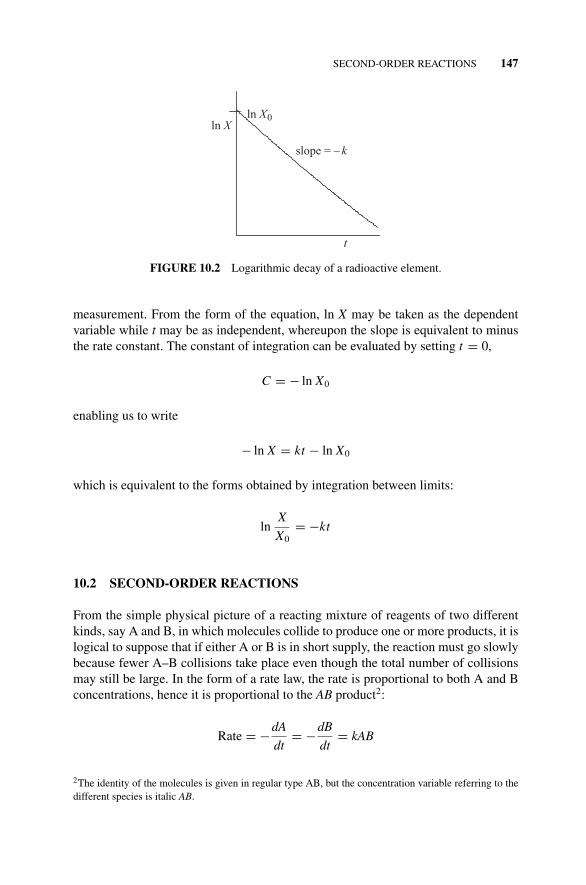
P1: OTA/XYZ P2: ABCc10 JWBS043-Rogers September 13, 2010 11:26 Printer Name: Yet to Come
SECOND-ORDER REACTIONS 147
ln Xln X0
t
slope = – k
FIGURE 10.2 Logarithmic decay of a radioactive element.
measurement. From the form of the equation, ln X may be taken as the dependentvariable while t may be as independent, whereupon the slope is equivalent to minusthe rate constant. The constant of integration can be evaluated by setting t = 0,
C = − ln X0
enabling us to write
− ln X = kt − ln X0
which is equivalent to the forms obtained by integration between limits:
lnX
X0= −kt
10.2 SECOND-ORDER REACTIONS
From the simple physical picture of a reacting mixture of reagents of two differentkinds, say A and B, in which molecules collide to produce one or more products, it islogical to suppose that if either A or B is in short supply, the reaction must go slowlybecause fewer A–B collisions take place even though the total number of collisionsmay still be large. In the form of a rate law, the rate is proportional to both A and Bconcentrations, hence it is proportional to the AB product2:
Rate = −dA
dt= −dB
dt= kAB
2The identity of the molecules is given in regular type AB, but the concentration variable referring to thedifferent species is italic AB.
P1: OTA/XYZ P2: ABCc10 JWBS043-Rogers September 13, 2010 11:26 Printer Name: Yet to Come
148 CHEMICAL KINETICS
If the reactants are mixed so that the initial concentrations A and B are equal, they willremain equal throughout, because for each molecule of one that reacts, a molecule ofthe other has also reacted. As a result, AB = A2 throughout, giving the special caseof the rate equation
−dA
dt= kAB = kA2
and
dA
A2= −k dt
Integrating∫
1
A2dA = −k
∫dt
gives
− 1
A= −kt + C
To evaluate the constant of integration, let t = 0. The concentration A is its initial
value A0, so − 1
A0= C and
1
A= kt + 1
A0
which leads to
A0 − A
A0 A= kt
The relation between t1/2 and k for this restricted form of the second-order reactionis kt1/2 A0 = 1.
An example of second-order kinetics in which the rate law −dA/dt = kAB = kA2
applies is the thermal decomposition of NO2:
2NO2(g) → 2NO(g) + O2(g)
The rate is controlled by collisions of NO2 molecules with other NO2 molecules,hence the stipulation A = B throughout is met. Although in this case the order ofthe reaction is the same as the stoichiometric coefficient, that need not be the case asexemplified by the thermal decomposition of N2O5:
2N2O5(g) → 4NO2(g) + O2(g)
which is first order.
P1: OTA/XYZ P2: ABCc10 JWBS043-Rogers September 13, 2010 11:26 Printer Name: Yet to Come
OTHER REACTION ORDERS 149
10.3 OTHER REACTION ORDERS
In general, the order of a chemical reaction is the sum of the exponents in the rateequation a + b + c + · · ·:
−dA
dt= kAa BbCc . . .
The order may be fractional or even decimal, but it is not a large number. Zero- andthird-order reactions exist, but they are not common. A zero-order reaction is one inwhich the rate does not vary with time:
d A
dt= k
This rate law might be followed by a reaction depending on some constant like thesurface area of a catalyst on which the reaction is taking place.
There are systematic mathematical methods for determining the order of a reactionfrom a data set of concentration vs. time even when the order is not simple.
10.3.1 Mathematical Interlude: The Laplace Transform
The Laplace transform is used to simplify differential equations. For the functionF(t) where t is the time and F(t) is zero at t < 0, the Laplace transform f (s) of F(t)is defined as
f (s) = L [F(t)] =∫ ∞
0e−st F(t) dt
The inverse Laplace transform of f (s) is F(t). The Laplace transform L [F(t)] is afunction of a function; it is called a functional. Extensive tables of Laplace transformsand inverse Laplace transforms are available (CRC Handbook of Chemistry andPhysics 2008–2009, 89th ed.).
First we shall convert the derivative of the function F(t) to a simple algebraicform. By definition,
L
[dF(t)
dt
]=
∫ ∞
0e−st dF(t)
dtdt
Integration by parts gives
L
[dF(t)
dt
]= F(t)e−st
∣∣∞0 −
∫ ∞
0F(t)d(e−st )
= −F(t = 0) + s∫ ∞
0F(t)e−st dt
= −F(t = 0) + s f (s)
P1: OTA/XYZ P2: ABCc10 JWBS043-Rogers September 13, 2010 11:26 Printer Name: Yet to Come
150 CHEMICAL KINETICS
10.3.2 Back to Kinetics: Sequential Reactions
In this section we shall obtain the concentration B in the a sequence of two first-orderreactions:
Ak1→ B
k2→ C
The differential equations are
dA
dt= −k1 A
dB
dt= k1 A − k2 B
dC
dt= k2 B
From the first equation, we have
A = A0e−k1t , B0 = C0 = 0
where the subscripted 0 indicates the initial concentration. Substituting this resultinto the equation for B(t), we obtain
dB(t)
dt= k1 A0e−k1t − k2 B(t)
Now take the Laplace transform of both sides and solve for b(s), the transform ofB(t):
sb(s) − B(t = 0) = k1 A0
s + k1− k2b(s)
where B(t = 0) = B0 = 0, so the remaining terms are
sb(s) + k2b(s) = k1 A0
s + k1
b(s) (s + k2) = k1 A0
s + k1
b(s) = k1 A0
s + k1
1
(s + k2)= k1 A0
1
(s + k1)
1
(s + k2)
P1: OTA/XYZ P2: ABCc10 JWBS043-Rogers September 13, 2010 11:26 Printer Name: Yet to Come
OTHER REACTION ORDERS 151
which is our solution for the Laplace transform of both sides of the rate equation. Nowtake the inverse Laplace transform. The Laplace transform b(s) inverse transforms,
of course, to B(t) and the inverse transform of1
(s + k1)
1
(s + k2)is
1
(s + k1)
1
(s + k2)inv transform−→ 1
k1 − k2
(e−k1t − e−k2t
)
so
B(t) = k1 A01
k1 − k2
(e−k1t − e−k2t
)
10.3.3 Reversible Reactions
No reaction goes to completion. Reactions we call “complete” are those in whichthe concentration of, for example, reactant A is negligible or not detectable in thereaction
A → B
This is the case when the standard free energy of A is much larger than that of B, sothat the reaction is accompanied by a significant decrease in free energy and leads toB more stable than A.
In many cases, something closer to a free energy balance exists. We write thereaction as an equilibrium characterized by an equilibrium constant Keq (Chapter 7).Kinetic rate constants k f and kb for forward and back reactions compete to establishthe equilibrium balance:
Ak f→←kb
B
k f
kb= Keq = B
A
When A and B are mixed in concentrations A and B that are not the equilibriumconcentrations, either the forward or the back reaction is faster than the other and thesystem is displaced so as to approach equilibrium.
The rate of depletion of A,
(−d A
dt
)obs
= k f A − kb B
is smaller than the rate that would be found if the reaction went to completion or ifwe had some mechanism for removal of B immediately as it is formed. The rate of
P1: OTA/XYZ P2: ABCc10 JWBS043-Rogers September 13, 2010 11:26 Printer Name: Yet to Come
152 CHEMICAL KINETICS
approach to equilibrium is always less than either the forward reaction or the backreaction because k f and kb work in opposition to one another.
For simple reversible systems,
A →← B
A + B →← C
A + B →← C + D
etc.
equations can be worked out that relate the observed rate constant kobs for the approachto equilibrium to k f and kb, the elementary reactions that contribute to it (Metiu,2006).
The concept of equilibrium as the result of opposite forward and back reactions iscalled the principle of detailed balance; for example, at equilibrium,
k f A − kb B = 0
The equations implied by the principle of detailed balance rest on the assumption thatthe concentrations of reactant and product vary in the simplest possible way. Thisassumption is often violated and must never be taken for granted.
Some enzyme-catalyzed reactions, including the famous Michaelis–Menten(Houston, 2001) mechanism, are examples of more complicated reaction mecha-nisms. Despite their complexity, they can often be broken down into elementary stepsand equilibriums. The kinetics of complex reactions can sometimes be simplified byregarding one component of the reaction as a constant during part of the chemicalprocess. This is the steady-state approximation (Metiu, 2006).
An especially important class of reaction mechanisms is that of the chain reactionsin which one molecular event leads to many, possibly very many, products. The classicexample for chemists is production of HBr from the elements:
H2 + Br2 → 2HBr
for which we might guess the rate law to be
1
2
d [HBr]
dt= k [H2] [Br2] wrong
but that guess would be wrong. Instead, the rate law is
1
2
d [HBr]
dt= k [H2] [Br2]1/2 right

P1: OTA/XYZ P2: ABCc10 JWBS043-Rogers September 13, 2010 11:26 Printer Name: Yet to Come
OTHER REACTION ORDERS 153
An acceptable mechanism for this reaction depends upon three elementary reactiontypes, initiation, chain, and termination:
Initiation Br2 + Mk1→ 2Br · + M
Chain Br· + H2k2→ HBr + H·
Chain H· + Br2k3→ HBr + Br·
Termination Br· + Br· k−1→ Br2
The point of this proposed mechanism is that the cyclic chain steps can continueindefinitely because the Br· free radicals used in the first chain step are produced in thesecond chain step. Initiation can be by a rather unlikely process such as collision witha high-energy molecule M in the first step or impact of a photon from a flame or sparkas in chain explosions. Though initiation may not occur very often, it can have a largeeffect. A hydrogen–oxygen explosion is an example. A very small spark can causea very large explosion. The HBr chain, though it may yield many molecules for oneinitiation step, does not, of course, go on forever. Some step such as recombination ofthe Br· free radicals terminates the chain or we run out of Br2 or H2 and the reactionstops.
If we assume that initiation and termination are rare events by comparison to thechain steps, for every Br· used up in the first step of the chain, one is produced inthe second chain step, so the amount of free radical present at any time during thereaction is constant:
d [Br·]dt
= 0
This is an example of the steady-state hypothesis. Making this assumption, a fewlines of algebra (Houston, 2006) lead to the correct rate equation given above:
1
2
d [HBr]
dt= k [H2] [Br2]1/2
If, by a more complicated mechanism, two or more reactive species are produced oneach step, the amount of reactive species may increase rapidly. For example, if tworeactive species are produced at each step, the geometric series, 1, 2, 4, 8, 16, . . . isfollowed. If the chain steps are fast, this kind of mechanism takes place with explosiveviolence. This type of mechanism is characteristic of nuclear fission bomb reactions.
Free radical and (controlled) chain reactions are also characteristic of some bio-chemical reactions, and they can behave in ways that are beneficial or detrimen-tal to the organism. A hydroperoxide RCOO· free radical chain may destroy lipidmolecules in a cell wall by lipid peroxidation with disastrous results for the cell.Free radicals derived from tocopherol (vitamin E) antioxidants act as sweepers in theblood, interfering with chain propagation, thereby slowing or preventing cell degra-dation. Free radicals have been detected in rapidly multiplying natal or neonatal cells
P1: OTA/XYZ P2: ABCc10 JWBS043-Rogers September 13, 2010 11:26 Printer Name: Yet to Come
154 CHEMICAL KINETICS
(beneficial) but they are also found in cancers undergoing uncontrolled reproduction.The biological role of free radicals is complex and not completely understood.
10.4 EXPERIMENTAL DETERMINATION OF THE RATE EQUATION
For some reactions, determination of the rate law and the rate constant may be assimple as mixing the reagents, titrating a sample of one of the reactants or antic-ipated products, waiting a while, titrating another sample, and so on, to obtain aseries of concentrations A, each at a time t. Treating this data set by an appropriatemathematical procedure gives the rate law and k.
Some of the most interesting contemporary research in kinetics involves trackingreaction components or intermediates by physical means, perhaps because they areof fleeting existence, being present in the reacting system for a second or less.
A straightforward approach to fairly fast reactions involves use of a stopped-flowreactor. One experimental design consists of two syringes connected to a mixer.To initiate the reaction, the syringes are driven simultaneously so that reactants Aand B flow into the mixer, are mixed thoroughly, and flow out of the mixer into atube where the reaction mixture is monitored by a spectrophotometer. The outputfrom the spectrophotometer is transmitted to a microcomputer at time intervals of,say, a few milliseconds or, perhaps, microseconds. The problem is well within thecapabilities of contemporary spectrophotometers and computer interfacing hardware,so the principal limiting factor is speed of mixing. Reactions with a half-time of amillisecond or less have been successfully studied in this way.
For very fast reactions, the limitation has been only the ingenuity of the researcherand flash photolysis studies of reactions with the astonishing half-time of t1/2 =10−15 s indicate that, for some people, this hasn’t been much of a limitation (Zewail,Nobel Prize, 1999, see Zewail, 1994).
10.5 REACTION MECHANISMS
The mechanism by which molecules actually combine is rarely as simple as the ratelaw suggests. Complex reactions may involve equilibriums,
A →← B
consecutive reactions,
A → B → C
parallel reactions,
A → C�B → D
or combinations of any or all of them.
P1: OTA/XYZ P2: ABCc10 JWBS043-Rogers September 13, 2010 11:26 Printer Name: Yet to Come
REACTION MECHANISMS 155
Because of these complications, the terms order and molecularity must be clearlydifferentiated. The order is the sum of exponents in the rate equation, while themolecularity is the number of molecules taking part in a simple reaction step.The order and molecularity will be the same in only the simplest reactions. Anexample in which the reaction order seems at first to be unrelated to the molecularityis the important atmospheric process involving ozone
2O3 → 3O2
which is not second order. Rather, it follows the rate law:
−d O3
dt= k
O23
O2
This can be explained by a reaction mechanism starting with a unimolecular step
O3 →← O2 + O
governed by the equilibrium constant
Keq = O2 O
O3
The second step of the proposed reaction mechanism is bimolecular
O + O3 → 2O2
and it is the slower step of the two. As in any sequential process, the slowest stepcontrols the rate of the entire process. In this case there are only two steps: a relativelyfast first step and a rate-controlling second step. The rate law for the bimolecularcollision between O and O3 is
−dO3
dt= k2OO3
Solving for O, we obtain
O = Keq O3
O2
Substituting for O in the previous equation,
−dO3
dt= k2OO3 = k2
Keq O3
O2O3 = k
O23
O2
we get the observed rate law and rate constant.
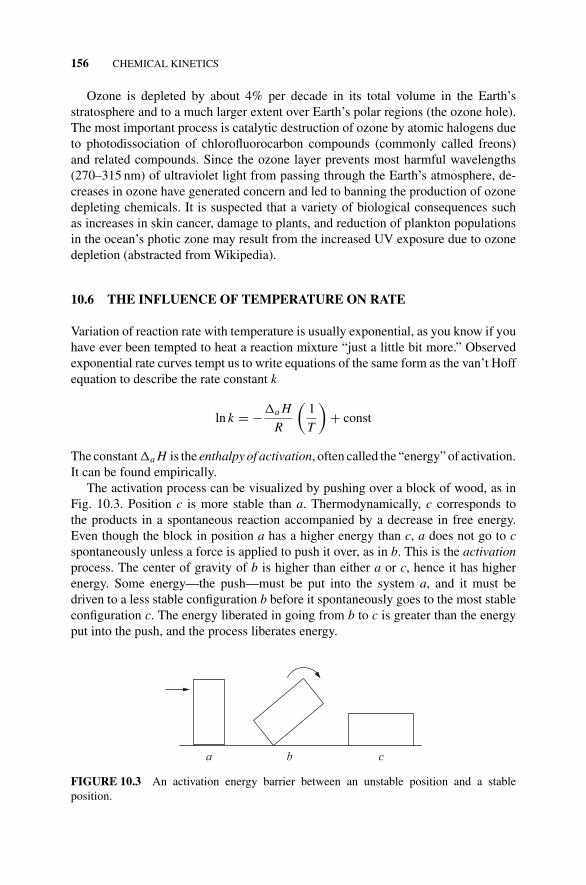
P1: OTA/XYZ P2: ABCc10 JWBS043-Rogers September 13, 2010 11:26 Printer Name: Yet to Come
156 CHEMICAL KINETICS
Ozone is depleted by about 4% per decade in its total volume in the Earth’sstratosphere and to a much larger extent over Earth’s polar regions (the ozone hole).The most important process is catalytic destruction of ozone by atomic halogens dueto photodissociation of chlorofluorocarbon compounds (commonly called freons)and related compounds. Since the ozone layer prevents most harmful wavelengths(270–315 nm) of ultraviolet light from passing through the Earth’s atmosphere, de-creases in ozone have generated concern and led to banning the production of ozonedepleting chemicals. It is suspected that a variety of biological consequences suchas increases in skin cancer, damage to plants, and reduction of plankton populationsin the ocean’s photic zone may result from the increased UV exposure due to ozonedepletion (abstracted from Wikipedia).
10.6 THE INFLUENCE OF TEMPERATURE ON RATE
Variation of reaction rate with temperature is usually exponential, as you know if youhave ever been tempted to heat a reaction mixture “just a little bit more.” Observedexponential rate curves tempt us to write equations of the same form as the van’t Hoffequation to describe the rate constant k
ln k = −�a H
R
(1
T
)+ const
The constant �a H is the enthalpy of activation, often called the “energy” of activation.It can be found empirically.
The activation process can be visualized by pushing over a block of wood, as inFig. 10.3. Position c is more stable than a. Thermodynamically, c corresponds tothe products in a spontaneous reaction accompanied by a decrease in free energy.Even though the block in position a has a higher energy than c, a does not go to cspontaneously unless a force is applied to push it over, as in b. This is the activationprocess. The center of gravity of b is higher than either a or c, hence it has higherenergy. Some energy—the push—must be put into the system a, and it must bedriven to a less stable configuration b before it spontaneously goes to the most stableconfiguration c. The energy liberated in going from b to c is greater than the energyput into the push, and the process liberates energy.
a b c
FIGURE 10.3 An activation energy barrier between an unstable position and a stableposition.
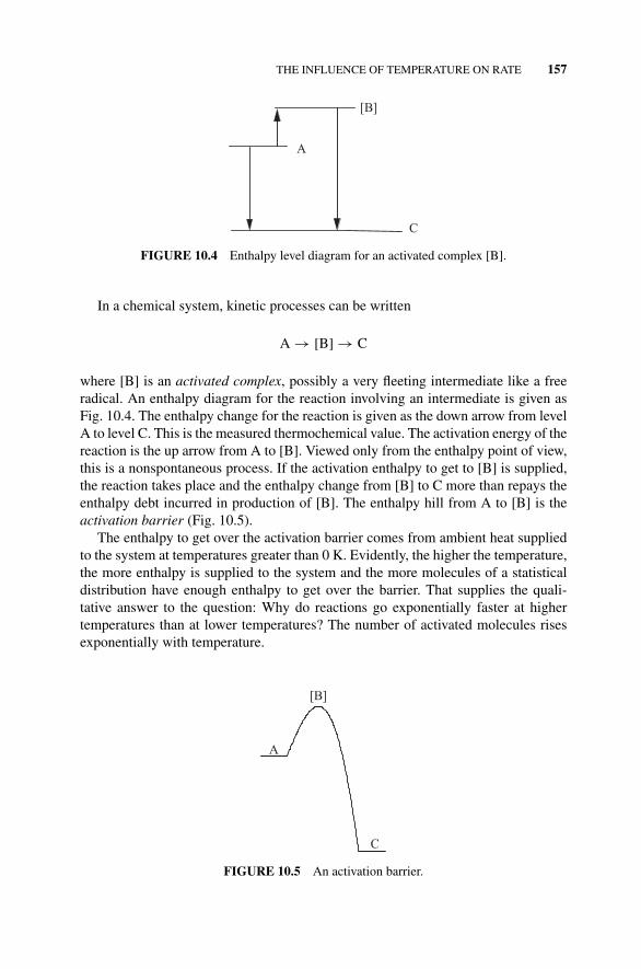
P1: OTA/XYZ P2: ABCc10 JWBS043-Rogers September 13, 2010 11:26 Printer Name: Yet to Come
THE INFLUENCE OF TEMPERATURE ON RATE 157
A
[B]
C
FIGURE 10.4 Enthalpy level diagram for an activated complex [B].
In a chemical system, kinetic processes can be written
A → [B] → C
where [B] is an activated complex, possibly a very fleeting intermediate like a freeradical. An enthalpy diagram for the reaction involving an intermediate is given asFig. 10.4. The enthalpy change for the reaction is given as the down arrow from levelA to level C. This is the measured thermochemical value. The activation energy of thereaction is the up arrow from A to [B]. Viewed only from the enthalpy point of view,this is a nonspontaneous process. If the activation enthalpy to get to [B] is supplied,the reaction takes place and the enthalpy change from [B] to C more than repays theenthalpy debt incurred in production of [B]. The enthalpy hill from A to [B] is theactivation barrier (Fig. 10.5).
The enthalpy to get over the activation barrier comes from ambient heat suppliedto the system at temperatures greater than 0 K. Evidently, the higher the temperature,the more enthalpy is supplied to the system and the more molecules of a statisticaldistribution have enough enthalpy to get over the barrier. That supplies the quali-tative answer to the question: Why do reactions go exponentially faster at highertemperatures than at lower temperatures? The number of activated molecules risesexponentially with temperature.
A
[B]
C
FIGURE 10.5 An activation barrier.
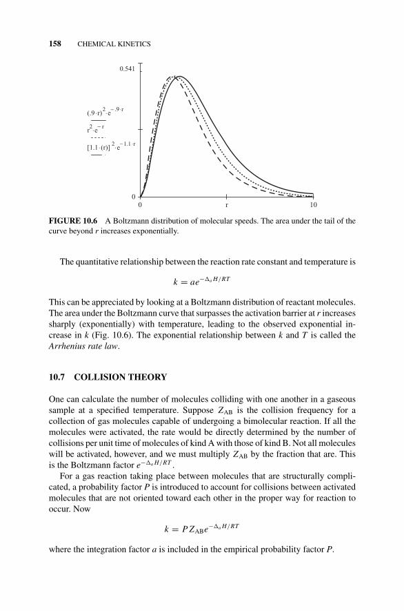
P1: OTA/XYZ P2: ABCc10 JWBS043-Rogers September 13, 2010 11:26 Printer Name: Yet to Come
158 CHEMICAL KINETICS
0.541
0
r)⋅(.92
e.9− r⋅⋅
r2
er−⋅
(r)]⋅[1.12
e1.1− r⋅⋅
10r0
FIGURE 10.6 A Boltzmann distribution of molecular speeds. The area under the tail of thecurve beyond r increases exponentially.
The quantitative relationship between the reaction rate constant and temperature is
k = ae−�a H/RT
This can be appreciated by looking at a Boltzmann distribution of reactant molecules.The area under the Boltzmann curve that surpasses the activation barrier at r increasessharply (exponentially) with temperature, leading to the observed exponential in-crease in k (Fig. 10.6). The exponential relationship between k and T is called theArrhenius rate law.
10.7 COLLISION THEORY
One can calculate the number of molecules colliding with one another in a gaseoussample at a specified temperature. Suppose ZAB is the collision frequency for acollection of gas molecules capable of undergoing a bimolecular reaction. If all themolecules were activated, the rate would be directly determined by the number ofcollisions per unit time of molecules of kind A with those of kind B. Not all moleculeswill be activated, however, and we must multiply ZAB by the fraction that are. Thisis the Boltzmann factor e−�a H/RT .
For a gas reaction taking place between molecules that are structurally compli-cated, a probability factor P is introduced to account for collisions between activatedmolecules that are not oriented toward each other in the proper way for reaction tooccur. Now
k = P ZABe−�a H/RT
where the integration factor a is included in the empirical probability factor P.
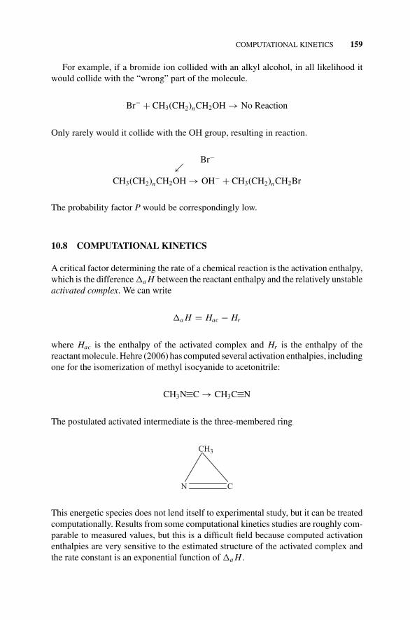
P1: OTA/XYZ P2: ABCc10 JWBS043-Rogers September 13, 2010 11:26 Printer Name: Yet to Come
COMPUTATIONAL KINETICS 159
For example, if a bromide ion collided with an alkyl alcohol, in all likelihood itwould collide with the “wrong” part of the molecule.
Br− + CH3(CH2)nCH2OH → No Reaction
Only rarely would it collide with the OH group, resulting in reaction.
Br−↙CH3(CH2)nCH2OH → OH− + CH3(CH2)nCH2Br
The probability factor P would be correspondingly low.
10.8 COMPUTATIONAL KINETICS
A critical factor determining the rate of a chemical reaction is the activation enthalpy,which is the difference �a H between the reactant enthalpy and the relatively unstableactivated complex. We can write
�a H = Hac − Hr
where Hac is the enthalpy of the activated complex and Hr is the enthalpy of thereactant molecule. Hehre (2006) has computed several activation enthalpies, includingone for the isomerization of methyl isocyanide to acetonitrile:
CH3N C → CH3C N
The postulated activated intermediate is the three-membered ring
CH3
CN
This energetic species does not lend itself to experimental study, but it can be treatedcomputationally. Results from some computational kinetics studies are roughly com-parable to measured values, but this is a difficult field because computed activationenthalpies are very sensitive to the estimated structure of the activated complex andthe rate constant is an exponential function of �a H .
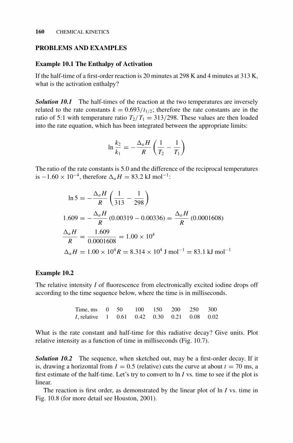
P1: OTA/XYZ P2: ABCc10 JWBS043-Rogers September 13, 2010 11:26 Printer Name: Yet to Come
160 CHEMICAL KINETICS
PROBLEMS AND EXAMPLES
Example 10.1 The Enthalpy of Activation
If the half-time of a first-order reaction is 20 minutes at 298 K and 4 minutes at 313 K,what is the activation enthalpy?
Solution 10.1 The half-times of the reaction at the two temperatures are inverselyrelated to the rate constants k = 0.693/t1/2; therefore the rate constants are in theratio of 5:1 with temperature ratio T2/T1 = 313/298. These values are then loadedinto the rate equation, which has been integrated between the appropriate limits:
lnk2
k1= −�a H
R
(1
T2− 1
T1
)
The ratio of the rate constants is 5.0 and the difference of the reciprocal temperaturesis −1.60 × 10⁻⁴, therefore �a H = 83.2 kJ mol−1:
ln 5 = −�a H
R
(1
313− 1
298
)
1.609 = −�a H
R(0.00319 − 0.00336) = �a H
R(0.0001608)
�a H
R= 1.609
0.0001608= 1.00 × 10⁴
�a H = 1.00 × 10⁴ R = 8.314 × 10⁴ J mol−1 = 83.1 kJ mol−1
Example 10.2
The relative intensity I of fluorescence from electronically excited iodine drops offaccording to the time sequence below, where the time is in milliseconds.
Time, ms 0 50 100 150 200 250 300I, relative 1 0.61 0.42 0.30 0.21 0.08 0.02
What is the rate constant and half-time for this radiative decay? Give units. Plotrelative intensity as a function of time in milliseconds (Fig. 10.7).
Solution 10.2 The sequence, when sketched out, may be a first-order decay. If itis, drawing a horizontal from I = 0.5 (relative) cuts the curve at about t = 70 ms, afirst estimate of the half-time. Let’s try to convert to ln I vs. time to see if the plot islinear.
The reaction is first order, as demonstrated by the linear plot of ln I vs. time inFig. 10.8 (for more detail see Houston, 2001).

P1: OTA/XYZ P2: ABCc10 JWBS043-Rogers September 13, 2010 11:26 Printer Name: Yet to Come
PROBLEMS AND EXAMPLES 161
Time (ms)
350300250200150100500R
elat
ive
Inte
nsity
0.0
0.2
0.4
0.6
0.8
1.0
1.2
FIGURE 10.7 First-order fluorescence decline from electronically excited iodine in mil-liseconds.
The statistical routine of the SigmaPlot C© 11.0 package gives, among other things,
Equation: Polynomial, Linear
f = y0 + a*x
Coefficient Std. Error
y0 0.0889 0.1232a −0.0098 0.0007
The intercept, given here as y0, is close to 0 as it should be and the slope, givenhere as a, is −0.0098 ms−1. This leads to a rate constant d I/dt = −k I of k =9.8 × 10⁻³ ms−1. The half-time for radiative decay is
t1/2 = ln 2
9.8 × 10⁻³ ms−1= .693
9.8 × 10⁻³ ms−1= 71 ms
Time (ms)3002001000
ln I
-3.5
-3.0
-2.5
-2.0
-1.5
-1.0
-0.5
0.0
0.5
FIGURE 10.8 The natural logarithm of relative intensity vs. time for radiative decay. Withinexperimental error, the plot is linear (Section 10.1).
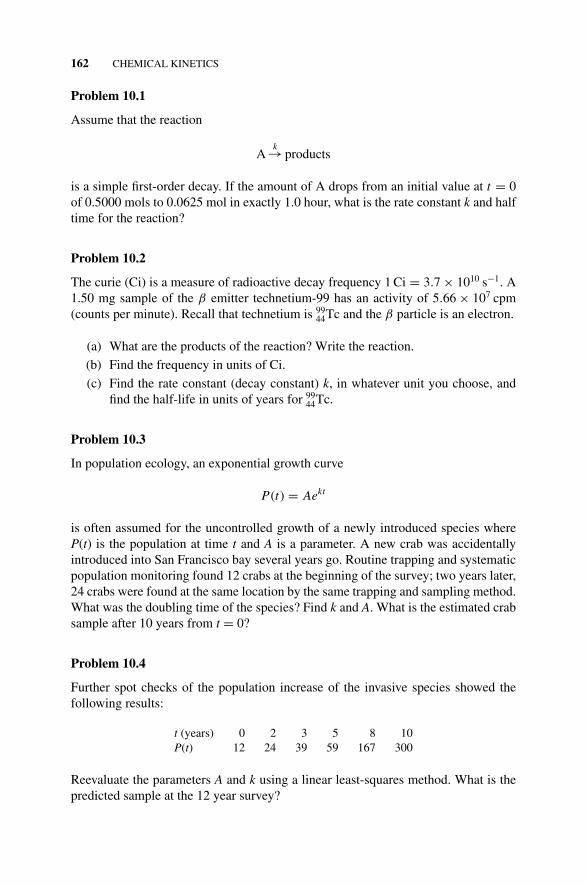
P1: OTA/XYZ P2: ABCc10 JWBS043-Rogers September 13, 2010 11:26 Printer Name: Yet to Come
162 CHEMICAL KINETICS
Problem 10.1
Assume that the reaction
Ak→ products
is a simple first-order decay. If the amount of A drops from an initial value at t = 0of 0.5000 mols to 0.0625 mol in exactly 1.0 hour, what is the rate constant k and halftime for the reaction?
Problem 10.2
The curie (Ci) is a measure of radioactive decay frequency 1 Ci = 3.7 × 10¹⁰ s−1. A1.50 mg sample of the β emitter technetium-99 has an activity of 5.66 × 10⁷ cpm(counts per minute). Recall that technetium is 99
44Tc and the β particle is an electron.
(a) What are the products of the reaction? Write the reaction.
(b) Find the frequency in units of Ci.
(c) Find the rate constant (decay constant) k, in whatever unit you choose, andfind the half-life in units of years for 99
44Tc.
Problem 10.3
In population ecology, an exponential growth curve
P(t) = Aekt
is often assumed for the uncontrolled growth of a newly introduced species whereP(t) is the population at time t and A is a parameter. A new crab was accidentallyintroduced into San Francisco bay several years go. Routine trapping and systematicpopulation monitoring found 12 crabs at the beginning of the survey; two years later,24 crabs were found at the same location by the same trapping and sampling method.What was the doubling time of the species? Find k and A. What is the estimated crabsample after 10 years from t = 0?
Problem 10.4
Further spot checks of the population increase of the invasive species showed thefollowing results:
t (years) 0 2 3 5 8 10P(t) 12 24 39 59 167 300
Reevaluate the parameters A and k using a linear least-squares method. What is thepredicted sample at the 12 year survey?
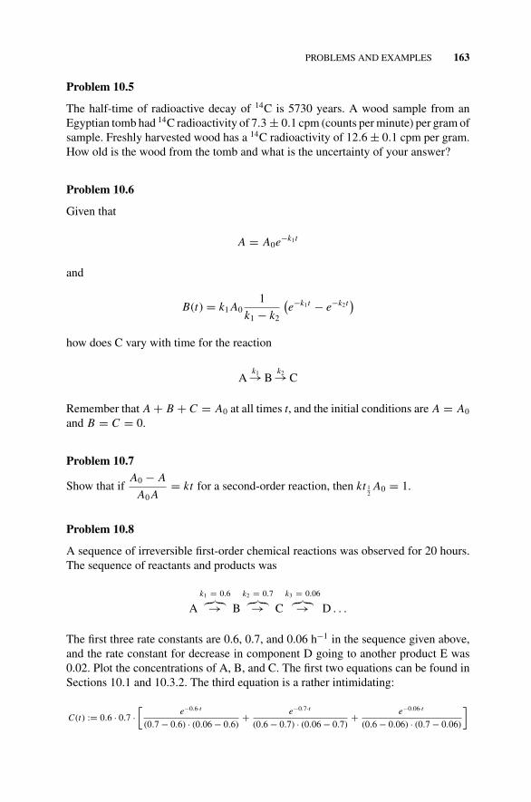
P1: OTA/XYZ P2: ABCc10 JWBS043-Rogers September 13, 2010 11:26 Printer Name: Yet to Come
PROBLEMS AND EXAMPLES 163
Problem 10.5
The half-time of radioactive decay of 14C is 5730 years. A wood sample from anEgyptian tomb had 14C radioactivity of 7.3 ± 0.1 cpm (counts per minute) per gram ofsample. Freshly harvested wood has a 14C radioactivity of 12.6 ± 0.1 cpm per gram.How old is the wood from the tomb and what is the uncertainty of your answer?
Problem 10.6
Given that
A = A0e−k1t
and
B(t) = k1 A01
k1 − k2
(e−k1t − e−k2t
)
how does C vary with time for the reaction
Ak1→ B
k2→ C
Remember that A + B + C = A0 at all times t, and the initial conditions are A = A0
and B = C = 0.
Problem 10.7
Show that ifA0 − A
A0 A= kt for a second-order reaction, then kt 1
2A0 = 1.
Problem 10.8
A sequence of irreversible first-order chemical reactions was observed for 20 hours.The sequence of reactants and products was
Ak1 = 0.6︷︸︸︷→ B
k2 = 0.7︷︸︸︷→ Ck3 = 0.06︷︸︸︷→ D . . .
The first three rate constants are 0.6, 0.7, and 0.06 h−1 in the sequence given above,and the rate constant for decrease in component D going to another product E was0.02. Plot the concentrations of A, B, and C. The first two equations can be found inSections 10.1 and 10.3.2. The third equation is a rather intimidating:
C(t) := 0.6 · 0.7 ·[
e−0.6·t
(0.7 − 0.6) · (0.06 − 0.6)+ e−0.7·t
(0.6 − 0.7) · (0.06 − 0.7)+ e−0.06·t
(0.6 − 0.06) · (0.7 − 0.06)
]
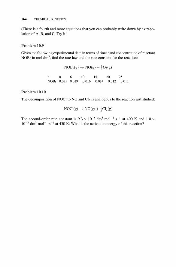
P1: OTA/XYZ P2: ABCc10 JWBS043-Rogers September 13, 2010 11:26 Printer Name: Yet to Come
164 CHEMICAL KINETICS
(There is a fourth and more equations that you can probably write down by extrapo-lation of A, B, and C. Try it!
Problem 10.9
Given the following experimental data in terms of time t and concentration of reactantNOBr in mol dm3, find the rate law and the rate constant for the reaction:
NOBr(g) → NO(g) + 12 O2(g)
t 0 6 10 15 20 25NOBr 0.025 0.019 0.016 0.014 0.012 0.011
Problem 10.10
The decomposition of NOCl to NO and Cl2 is analogous to the reaction just studied:
NOCl(g) → NO(g) + 12 Cl2(g)
The second-order rate constant is 9.3 × 10⁻⁵ dm3 mol−1 s−1 at 400 K and 1.0 ×10⁻³ dm3 mol−1 s−1 at 430 K. What is the activation energy of this reaction?
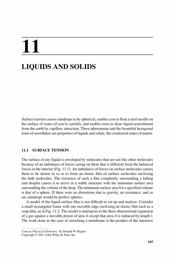
P1: OTA/XYZ P2: ABCc11 JWBS043-Rogers September 13, 2010 11:26 Printer Name: Yet to Come
11LIQUIDS AND SOLIDS
Surface tension causes raindrops to be spherical, enables you to float a steel needle onthe surface of water (if you’re careful), and enables trees to draw liquid nourishmentfrom the earth by capillary attraction. These phenomena and the beautiful hexagonalform of snowflakes are properties of liquids and solids, the condensed states of matter.
11.1 SURFACE TENSION
The surface of any liquid is enveloped by molecules that are not like other moleculesbecause of an imbalance of forces acting on them that is different from the balancedforces in the interior (Fig. 11.1). An imbalance of forces on surface molecules causesthem to be drawn in so as to form an elastic film of surface molecules enclosingthe bulk molecules. The existence of such a film completely surrounding a fallingrain droplet causes it to arrive at a stable structure with the minimum surface areasurrounding the volume of the drop. The minimum surface area for a specified volumeis that of a sphere. If there were no distortions due to gravity, air resistance, and soon, raindrops would be perfect spheres.
A model of the liquid surface film is not difficult to set up and analyze. Considera small rectangular frame with one movable edge enclosing an elastic film such as asoap film, as in Fig. 11.2. The model is analogous to the three-dimensional expansionof a gas against a movable piston of area A except that area A is replaced by length l.The work done in the case of stretching a membrane is the product of the intensive
Concise Physical Chemistry, by Donald W. RogersCopyright C© 2011 John Wiley & Sons, Inc.
165
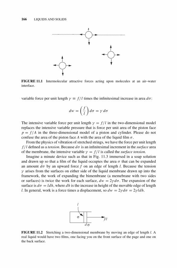
P1: OTA/XYZ P2: ABCc11 JWBS043-Rogers September 13, 2010 11:26 Printer Name: Yet to Come
166 LIQUIDS AND SOLIDS
FIGURE 11.1 Intermolecular attractive forces acting upon molecules at an air–waterinterface.
variable force per unit length γ ≡ f/ l times the infinitesimal increase in area dσ :
dw =(
f
l
)dσ = γ dσ
The intensive variable force per unit length γ = f/ l in the two-dimensional modelreplaces the intensive variable pressure that is force per unit area of the piston facep = f/A in the three-dimensional model of a piston and cylinder. Please do notconfuse the area of the piston face A with the area of the liquid film σ .
From the physics of vibration of stretched strings, we have the force per unit lengthf/ l defined as a tension. Because dσ is an infinitesimal increment in the surface areaof the membrane, the intensive variable γ = f/ l is called the surface tension.
Imagine a minute device such as that in Fig. 11.3 immersed in a soap solutionand drawn up so that a film of the liquid occupies the area σ that can be expandedan amount dσ by an upward force f on an edge of length l. Because the tensionγ arises from the surfaces on either side of the liquid membrane drawn up into theframework, the work of expanding the bimembrane (a memebrane with two sidesor surfaces) is twice the work for each surface, dw = 2γ dσ . The expansion of thesurface is dσ = ldh, where dh is the increase in height of the movable edge of lengthl. In general, work is a force times a displacement, so dw = 2γ dσ = 2γ ldh.
f/lσ
d σ
l
FIGURE 11.2 Stretching a two-dimensional membrane by moving an edge of length l. Areal liquid would have two films, one facing you on the front surface of the page and one onthe back surface.
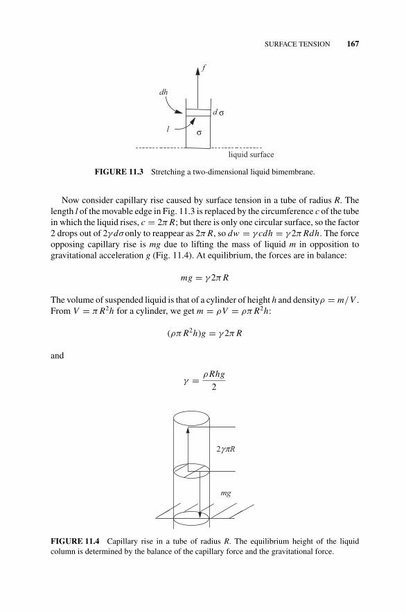
P1: OTA/XYZ P2: ABCc11 JWBS043-Rogers September 13, 2010 11:26 Printer Name: Yet to Come
SURFACE TENSION 167
liquid surface
f
σ
d σ
l
dh
FIGURE 11.3 Stretching a two-dimensional liquid bimembrane.
Now consider capillary rise caused by surface tension in a tube of radius R. Thelength l of the movable edge in Fig. 11.3 is replaced by the circumference c of the tubein which the liquid rises, c = 2π R; but there is only one circular surface, so the factor2 drops out of 2γ dσonly to reappear as 2π R, so dw = γ cdh = γ 2π Rdh. The forceopposing capillary rise is mg due to lifting the mass of liquid m in opposition togravitational acceleration g (Fig. 11.4). At equilibrium, the forces are in balance:
mg = γ 2π R
The volume of suspended liquid is that of a cylinder of height h and densityρ = m/V .From V = π R2h for a cylinder, we get m = ρV = ρπ R2h:
(ρπ R2h)g = γ 2π R
and
γ = ρRhg
2
mg
2γπR
FIGURE 11.4 Capillary rise in a tube of radius R. The equilibrium height of the liquidcolumn is determined by the balance of the capillary force and the gravitational force.
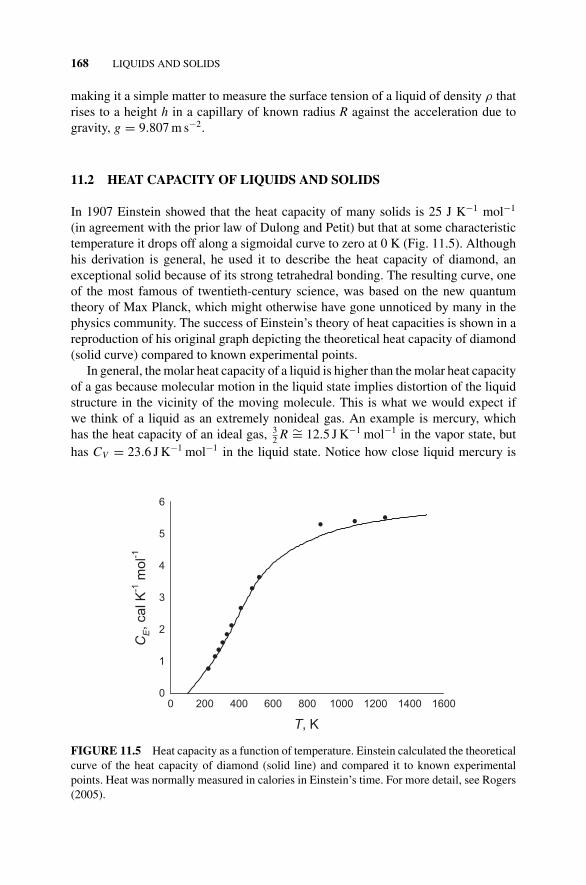
P1: OTA/XYZ P2: ABCc11 JWBS043-Rogers September 13, 2010 11:26 Printer Name: Yet to Come
168 LIQUIDS AND SOLIDS
making it a simple matter to measure the surface tension of a liquid of density ρ thatrises to a height h in a capillary of known radius R against the acceleration due togravity, g = 9.807 m s−2.
11.2 HEAT CAPACITY OF LIQUIDS AND SOLIDS
In 1907 Einstein showed that the heat capacity of many solids is 25 J K−1 mol−1
(in agreement with the prior law of Dulong and Petit) but that at some characteristictemperature it drops off along a sigmoidal curve to zero at 0 K (Fig. 11.5). Althoughhis derivation is general, he used it to describe the heat capacity of diamond, anexceptional solid because of its strong tetrahedral bonding. The resulting curve, oneof the most famous of twentieth-century science, was based on the new quantumtheory of Max Planck, which might otherwise have gone unnoticed by many in thephysics community. The success of Einstein’s theory of heat capacities is shown in areproduction of his original graph depicting the theoretical heat capacity of diamond(solid curve) compared to known experimental points.
In general, the molar heat capacity of a liquid is higher than the molar heat capacityof a gas because molecular motion in the liquid state implies distortion of the liquidstructure in the vicinity of the moving molecule. This is what we would expect ifwe think of a liquid as an extremely nonideal gas. An example is mercury, whichhas the heat capacity of an ideal gas, 3
2 R ∼= 12.5 J K−1 mol−1 in the vapor state, buthas CV = 23.6 J K−1 mol−1 in the liquid state. Notice how close liquid mercury is
T, K
16001400120010008006004002000
CE,
ca
l K
-1 m
ol-1
0
1
2
3
4
5
6
FIGURE 11.5 Heat capacity as a function of temperature. Einstein calculated the theoreticalcurve of the heat capacity of diamond (solid line) and compared it to known experimentalpoints. Heat was normally measured in calories in Einstein’s time. For more detail, see Rogers(2005).
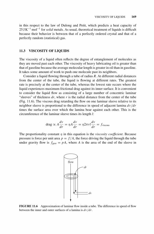
P1: OTA/XYZ P2: ABCc11 JWBS043-Rogers September 13, 2010 11:26 Printer Name: Yet to Come
VISCOSITY OF LIQUIDS 169
in this respect to the law of Dulong and Petit, which predicts a heat capacity of25 J K−1 mol−1 for solid metals. As usual, theoretical treatment of liquids is difficultbecause their behavior is between that of a perfectly ordered crystal and that of aperfectly random (statistical) gas.
11.3 VISCOSITY OF LIQUIDS
The viscosity of a liquid often reflects the degree of entanglement of molecules asthey are moved past each other. The viscosity of heavy lubricating oil is greater thanthat of gasoline because the average molecular length is greater in oil than in gasoline.It takes some amount of work to push one molecule past its neighbors.
Consider a liquid flowing through a tube of radius R. At different radial distancesfrom the center of the tube, the liquid is flowing at different rates. The greatestrate is precisely at the center of the tube, whereas the lowest rate occurs where theliquid experiences maximum frictional drag against its inner surface. It is convenientto consider the liquid flow as consisting of a large number of concentric laminar“sleeves” of thickness dr, where r is the radial distance from the center of the tube(Fig. 11.6). The viscous drag retarding the flow on one laminar sleeve relative to itsneighbor sleeve is proportional to the difference in speed of adjacent lamina dv/drtimes the surface area over which the lamina bear against each other. This is thecircumference of the laminar sleeve times its length l:
drag ∝ Adv
dr= ηA
dv
dr= η2πrl
dv
dr= fviscous
The proportionality constant η in this equation is the viscosity coefficient. Becausepressure is force per unit area p = f/A, the force driving the liquid through the tubeunder gravity flow is fgrav = p A, where A is the area of the end of the sleeve in
dr
dv
flow
FIGURE 11.6 Approximation of laminar flow inside a tube. The difference in speed of flowbetween the inner and outer surfaces of a lamina is dv/dr .
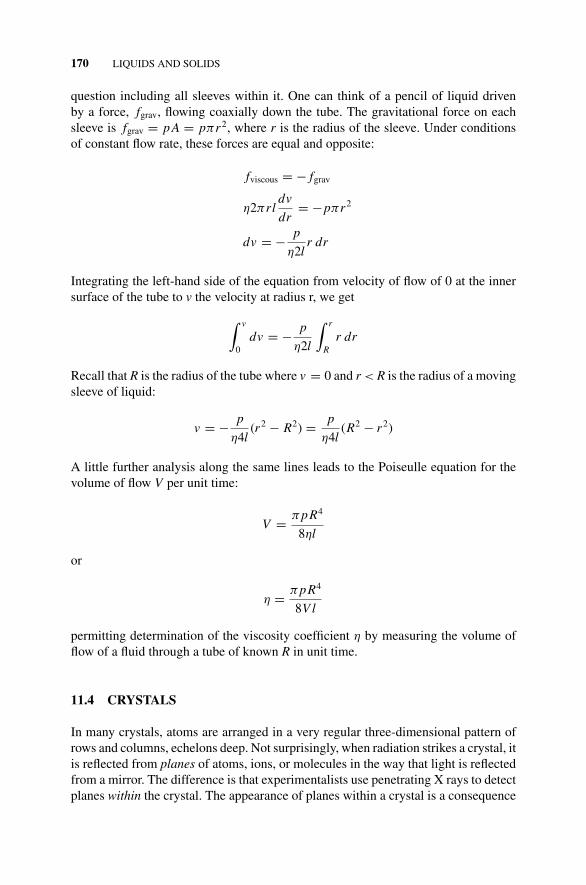
P1: OTA/XYZ P2: ABCc11 JWBS043-Rogers September 13, 2010 11:26 Printer Name: Yet to Come
170 LIQUIDS AND SOLIDS
question including all sleeves within it. One can think of a pencil of liquid drivenby a force, fgrav, flowing coaxially down the tube. The gravitational force on eachsleeve is fgrav = p A = pπr2, where r is the radius of the sleeve. Under conditionsof constant flow rate, these forces are equal and opposite:
fviscous = − fgrav
η2πrldv
dr= −pπr2
dv = − p
η2lr dr
Integrating the left-hand side of the equation from velocity of flow of 0 at the innersurface of the tube to v the velocity at radius r, we get
∫ v
0dv = − p
η2l
∫ r
Rr dr
Recall that R is the radius of the tube where v = 0 and r < R is the radius of a movingsleeve of liquid:
v = − p
η4l(r2 − R2) = p
η4l(R2 − r2)
A little further analysis along the same lines leads to the Poiseulle equation for thevolume of flow V per unit time:
V = πpR4
8ηl
or
η = πpR4
8V l
permitting determination of the viscosity coefficient η by measuring the volume offlow of a fluid through a tube of known R in unit time.
11.4 CRYSTALS
In many crystals, atoms are arranged in a very regular three-dimensional pattern ofrows and columns, echelons deep. Not surprisingly, when radiation strikes a crystal, itis reflected from planes of atoms, ions, or molecules in the way that light is reflectedfrom a mirror. The difference is that experimentalists use penetrating X rays to detectplanes within the crystal. The appearance of planes within a crystal is a consequence
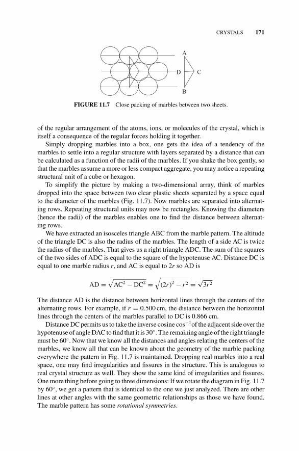
P1: OTA/XYZ P2: ABCc11 JWBS043-Rogers September 13, 2010 11:26 Printer Name: Yet to Come
CRYSTALS 171
A
B
CD
FIGURE 11.7 Close packing of marbles between two sheets.
of the regular arrangement of the atoms, ions, or molecules of the crystal, which isitself a consequence of the regular forces holding it together.
Simply dropping marbles into a box, one gets the idea of a tendency of themarbles to settle into a regular structure with layers separated by a distance that canbe calculated as a function of the radii of the marbles. If you shake the box gently, sothat the marbles assume a more or less compact aggregate, you may notice a repeatingstructural unit of a cube or hexagon.
To simplify the picture by making a two-dimensional array, think of marblesdropped into the space between two clear plastic sheets separated by a space equalto the diameter of the marbles (Fig. 11.7). Now marbles are separated into alternat-ing rows. Repeating structural units may now be rectangles. Knowing the diameters(hence the radii) of the marbles enables one to find the distance between alternat-ing rows.
We have extracted an isosceles triangle ABC from the marble pattern. The altitudeof the triangle DC is also the radius of the marbles. The length of a side AC is twicethe radius of the marbles. That gives us a right triangle ADC. The sum of the squaresof the two sides of ADC is equal to the square of the hypotenuse AC. Distance DC isequal to one marble radius r, and AC is equal to 2r so AD is
AD =√
AC2 − DC2 =√
(2r )2 − r2 =√
3r2
The distance AD is the distance between horizontal lines through the centers of thealternating rows. For example, if r = 0.500 cm, the distance between the horizontallines through the centers of the marbles parallel to DC is 0.866 cm.
Distance DC permits us to take the inverse cosine cos−1of the adjacent side over thehypotenuse of angle DAC to find that it is 30◦. The remaining angle of the right trianglemust be 60◦. Now that we know all the distances and angles relating the centers of themarbles, we know all that can be known about the geometry of the marble packingeverywhere the pattern in Fig. 11.7 is maintained. Dropping real marbles into a realspace, one may find irregularities and fissures in the structure. This is analogous toreal crystal structure as well. They show the same kind of irregularities and fissures.One more thing before going to three dimensions: If we rotate the diagram in Fig. 11.7by 60◦, we get a pattern that is identical to the one we just analyzed. There are otherlines at other angles with the same geometric relationships as those we have found.The marble pattern has some rotational symmetries.
P1: OTA/XYZ P2: ABCc11 JWBS043-Rogers September 13, 2010 11:26 Printer Name: Yet to Come
172 LIQUIDS AND SOLIDS
A
B
C
D
FIGURE 11.8 A less efficient packing of marbles. This packing is less efficient than closepacking because the same number of marbles take up a greater space. To see this most clearly,notice that the interstitial spaces are larger than they are in Fig. 11.7.
With difficulty, marbles might be juggled into a less efficient but still regularpattern like Fig. 11.8. The vertical distance between centers for 0.500 cm marblesis now twice the radius as compared to only 0.866 r for close packing. The samenumber of marbles take up more space.
Suppose we had some experimental method of determining distance betweenlayers DC. That would enable us to tell the difference between the packing pattern inFigs. 11.7 and 11.8. Assuming that atoms fall into a regular array when an elementor compound crystallizes, we can picture a laminar sheet of atoms with very densenuclei in an array similar to that Fig. 11.7 or 11.8. If marbles were packed into a three-dimensional box, the packing pattern determination would be very closely analogousto the pattern determination for marbles restricted to a plane. They would pack ina more or less regular way, and different packing patterns would be a more or lessefficient with respect to space use, just as the marbles were in the simple illustrativecase of two dimensions. Atoms, molecules, or ions pack in three-dimensional crystalsas well. We would like to have an experimental method to solve the reverse of theproblem we just solved; from an experimental value for the distance between layersof atoms, we would like to obtain the radius of the atoms themselves. The object ofX-ray crystallography is to determine the distances and angles between atomic centersas we have done with marbles. The problem may be much more complicated, as inthe example of proteins, or it may be nearly as simple as the method just describedextrapolated to there dimensions, as in the case of pure metals and ionic salts.
Electromagnetic waves, from radio frequency of meter wavelengths to γ rays ofλ ≈ 0.1 nm, have an electrical and a magnetic component. The radiation can bedescribed mathematically as two sine waves, one electrical ε and the other magneticH, describing two oscillating vector fields oriented at right angles to one another.For constructive interference between two waves, the field vectors must point in thesame direction. Otherwise, the radiation of one wave dims or obliterates the other bydestructive interference.
Figure 11.9 shows that, for the radiation reflected from two adjacent horizontallines of atoms to be in phase (to have their arrows pointed in the same direction),the difference in path must be an integer multiple of the wavelength λ. The pathdifference is shown as a heavy line. A path difference that is twice the wavelengthof incoming radiation will interfere constructively, and one that is three times λ
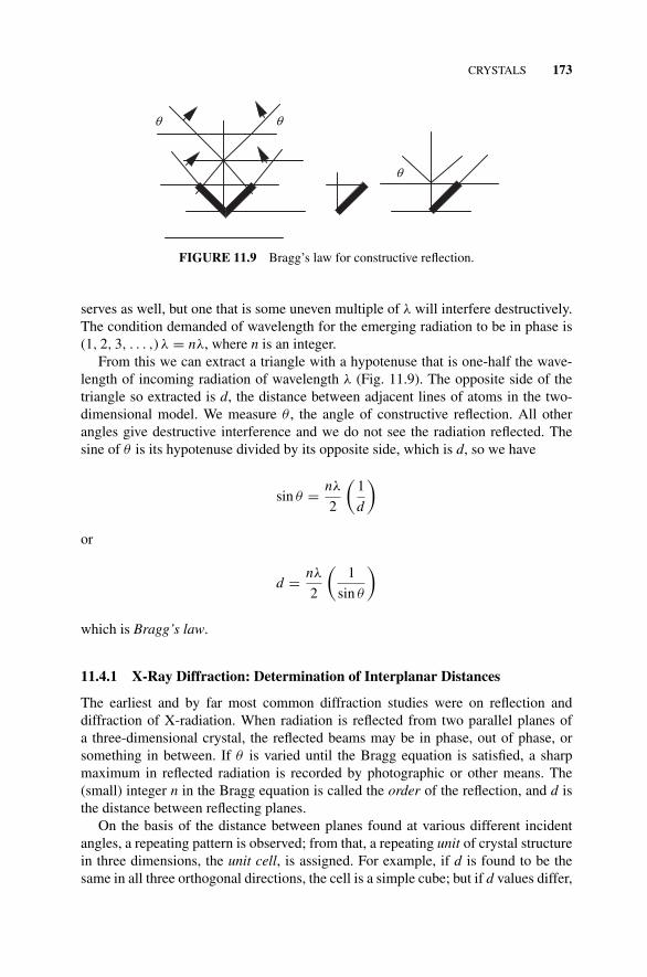
P1: OTA/XYZ P2: ABCc11 JWBS043-Rogers September 13, 2010 11:26 Printer Name: Yet to Come
CRYSTALS 173
θ
θ θ
FIGURE 11.9 Bragg’s law for constructive reflection.
serves as well, but one that is some uneven multiple of λ will interfere destructively.The condition demanded of wavelength for the emerging radiation to be in phase is(1, 2, 3, . . . ,) λ = nλ, where n is an integer.
From this we can extract a triangle with a hypotenuse that is one-half the wave-length of incoming radiation of wavelength λ (Fig. 11.9). The opposite side of thetriangle so extracted is d, the distance between adjacent lines of atoms in the two-dimensional model. We measure θ , the angle of constructive reflection. All otherangles give destructive interference and we do not see the radiation reflected. Thesine of θ is its hypotenuse divided by its opposite side, which is d, so we have
sin θ = nλ
2
(1
d
)
or
d = nλ
2
(1
sin θ
)
which is Bragg’s law.
11.4.1 X-Ray Diffraction: Determination of Interplanar Distances
The earliest and by far most common diffraction studies were on reflection anddiffraction of X-radiation. When radiation is reflected from two parallel planes ofa three-dimensional crystal, the reflected beams may be in phase, out of phase, orsomething in between. If θ is varied until the Bragg equation is satisfied, a sharpmaximum in reflected radiation is recorded by photographic or other means. The(small) integer n in the Bragg equation is called the order of the reflection, and d isthe distance between reflecting planes.
On the basis of the distance between planes found at various different incidentangles, a repeating pattern is observed; from that, a repeating unit of crystal structurein three dimensions, the unit cell, is assigned. For example, if d is found to be thesame in all three orthogonal directions, the cell is a simple cube; but if d values differ,
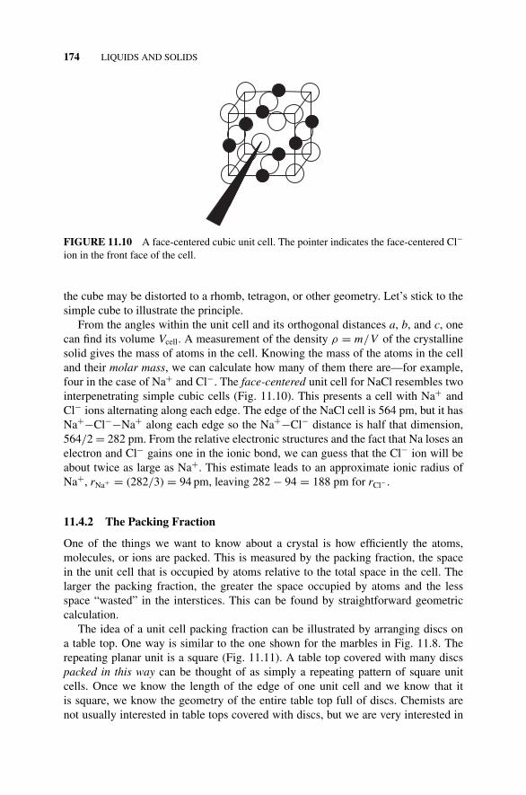
P1: OTA/XYZ P2: ABCc11 JWBS043-Rogers September 13, 2010 11:26 Printer Name: Yet to Come
174 LIQUIDS AND SOLIDS
FIGURE 11.10 A face-centered cubic unit cell. The pointer indicates the face-centered Cl−
ion in the front face of the cell.
the cube may be distorted to a rhomb, tetragon, or other geometry. Let’s stick to thesimple cube to illustrate the principle.
From the angles within the unit cell and its orthogonal distances a, b, and c, onecan find its volume Vcell. A measurement of the density ρ = m/V of the crystallinesolid gives the mass of atoms in the cell. Knowing the mass of the atoms in the celland their molar mass, we can calculate how many of them there are—for example,four in the case of Na+ and Cl−. The face-centered unit cell for NaCl resembles twointerpenetrating simple cubic cells (Fig. 11.10). This presents a cell with Na+ andCl− ions alternating along each edge. The edge of the NaCl cell is 564 pm, but it hasNa+−Cl−−Na+ along each edge so the Na+−Cl− distance is half that dimension,564/2 = 282 pm. From the relative electronic structures and the fact that Na loses anelectron and Cl− gains one in the ionic bond, we can guess that the Cl− ion will beabout twice as large as Na+. This estimate leads to an approximate ionic radius ofNa+, rNa+ = (282/3) = 94 pm, leaving 282 − 94 = 188 pm for rCl− .
11.4.2 The Packing Fraction
One of the things we want to know about a crystal is how efficiently the atoms,molecules, or ions are packed. This is measured by the packing fraction, the spacein the unit cell that is occupied by atoms relative to the total space in the cell. Thelarger the packing fraction, the greater the space occupied by atoms and the lessspace “wasted” in the interstices. This can be found by straightforward geometriccalculation.
The idea of a unit cell packing fraction can be illustrated by arranging discs ona table top. One way is similar to the one shown for the marbles in Fig. 11.8. Therepeating planar unit is a square (Fig. 11.11). A table top covered with many discspacked in this way can be thought of as simply a repeating pattern of square unitcells. Once we know the length of the edge of one unit cell and we know that itis square, we know the geometry of the entire table top full of discs. Chemists arenot usually interested in table tops covered with discs, but we are very interested in

P1: OTA/XYZ P2: ABCc11 JWBS043-Rogers September 13, 2010 11:26 Printer Name: Yet to Come
CRYSTALS 175
FIGURE 11.11 A two-dimensional unit cell for packing of discs.
the three-dimensional structure of atomic, molecular, and ionic solids in the regulararrangements we find in crystals. The concept of the unit cell is central in X-raycrystallography.
A crystal with the simple square atomic or molecular packing arrangement in allthree directions is completely described as a repeating three-dimensional pattern ofcubic unit cells. Once we know the length of the edge of the cubic unit cell, we knowthe geometry of the entire crystal (aside from impurities and structural imperfections).
The three-dimensional analog of Fig. 11.11 has a simple cubic unit cell(Fig. 11.12).
To simplify, let us go back to the unit cell of discs in Fig. 11.11. The total area A ofdiscs within the cell is 4 times A/4, where A = πr2 because, although there are fourdiscs, one on each corner of the cell, only one-fourth of each disc is actually insidethe cell. The dimension of the cell itself is 2r on an edge so the area of the unit cell is(2r )2 = 4π2. The area of the discs within the cell is πr2, so the packing fraction is
P = Adisc
Acell= πr2
4r2= π
4= 0.785
When this structure is taken to a three-dimensional simple cubic structure, the inter-stitial space at the center of the cube takes a larger proportion of the whole and thepacking fraction is a rather inefficient 0.52. Simple cubic packing is not favored bymany crystals. An exception is the metal polonium, 84Po.
FIGURE 11.12 A simple cubic cell.
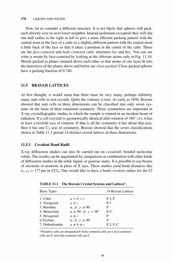
P1: OTA/XYZ P2: ABCc11 JWBS043-Rogers September 13, 2010 11:26 Printer Name: Yet to Come
176 LIQUIDS AND SOLIDS
Now, let us consider a different structure. It is not likely that spheres will pack,each directly over its next lower neighbor. Instead (polonium excepted) they will slipone-half radius to the right or left to give a more efficient packing pattern with thecentral atom in the face of a cube or a slightly different pattern with the central atoma little back of the face so that it takes a position in the center of the cube. Theseare the face-centered and body-centered cubic structures fcc and bcc. You can seewhat is meant by face-centered by looking at the chlorine atoms only in Fig. 11.10.Metals packed as planes situated above each other so that atoms of one layer fit intothe interstices of the planes above and below are close-packed. Close-packed sphereshave a packing fraction of 0.740.
11.5 BRAVAIS LATTICES
At first thought, it would seem that there must be very many, perhaps infinitelymany, unit cells in real crystals. Quite the contrary is true. As early as 1850, Bravaisshowed that unit cells in three dimensions can be classified into only seven sys-tems on the basis of their rotational symmetry. These symmetries are important inX-ray crystallographic studies in which the sample is rotated in an incident beam ofradiation. If a cell (crystal) is geometrically identical after rotation of 180◦ (π ), it hasat least a twofold axis of rotation. If that is all the symmetry it has about that axis,then it has one C2 axis of symmetry. Bravais showed that the seven classificationsshown in Table 11.1 permit 14 distinct crystal lattices in three dimensions.
11.5.1 Covalent Bond Radii
X-ray diffraction studies can also be carried out on covalently bonded molecularsolids. The results can be augmented by comparison or combination with other kindsof diffraction studies in the solid, liquid, or gaseous states. It is possible to use beamsof electrons or neutrons in place of X rays. These studies yield bond distances likerC−Cl = 177 pm in CCl4. One would like to have a bond covalent radius for the Cl
TABLE 11.1 The Bravais Crystal Systems and Latticesa.
Basic Types 14 Bravais Lattices
1. Cubic a = b = c P, I, F2. Tetragonal a �= c P, I3. Rhombic α, β, γ �= 90◦ P4. Monoclinic α �= 90◦ β, γ = 90◦ P, C5. Hexagonal a �= c P6.Triclinic α, β, γ �= 90◦ P7. Orthorhombic a �= b �= c P, I, F, C
aPrimitive cells are designated P, body-centered cells are I, face-centeredcells are F, and side-centered cells are C.
P1: OTA/XYZ P2: ABCc11 JWBS043-Rogers September 13, 2010 11:26 Printer Name: Yet to Come
LATTICE ENERGIES 177
atom in CCl4, for example, but there is no clear way of finding where, along the C–Clbond axis, one radius leaves off and the other begins.
One approach to this difficulty is by finding the homonuclear bond distances inmolecules like ethane for which the C–C bond distance is 154 pm, and Cl–Cl for whichit is 200 pm. Under the assumption that homonuclear bond distances will be carriedover into the heteronuclear cases, one has (200/2 + 154/2) = 100 + 77 = 177 pm,which successfully reproduces the experimental value for rC−Cl. Now, by studyingother compounds involving C and other compounds involving Cl, one can graduallybuild up tables of covalent bond radii such as those found in elementary textbooks(Ebbing and Gammon, 1999).
A number of points should be considered before using bond lengths or atomicradii. For one thing, combination of X-ray data with neutron diffraction data is riskybecause X-radiation is scattered by the electron cloud surrounding the nuclei in themolecule and neutrons are scattered by the nuclei themselves. Clearly the first isuseful in studying bonds and the second is useful for structure. Also, there is noreason to expect ionic radii and covalent radii to agree with one another because ofthe different modes of chemical bonding involved. Tables of bond distances, ionicradii, and covalent radii should be used with some degree of reserve because ofpotential inconsistencies and approximations.
11.6 COMPUTATIONAL GEOMETRIES
Most present-day molecular structure–energy computer programs contain a routinethat optimizes the geometry of the molecule under study so that each of the constituentatoms resides at the bottom of its unique potential energy well. Once knowing thecomplete molecular geometry, the bond lengths and angles can be calculated withgreat precision. The results, however, are not exactly comparable to experimental databecause the energy minimum found by computational optimization for atoms in theforce field of all other nuclei and electrons does not coincide with the average positionof the vibrating atom. Current estimates of atomic radii and bond lengths are in goodagreement overall but differ slightly according to the method used to determine them.Using the Spartan C© package, the homonuclear distance rH−H = 73.6 pm and theheteronuclear distance rH−F = 90.0 pm are found, as compared to the experimentalvalues of 74.2 and 91.7 pm.
11.7 LATTICE ENERGIES
Along with their geometry, we would like to know how firmly ionic crystals areheld together. A quantitative measure of the energy or enthalpy holding the crystaltogether is its lattice energy. The lattice energy is the energy necessary to draw ionsout of the crystal lattice and propel them into the gaseous state.
NaI(crystal) → Na+(g) + I−(g)
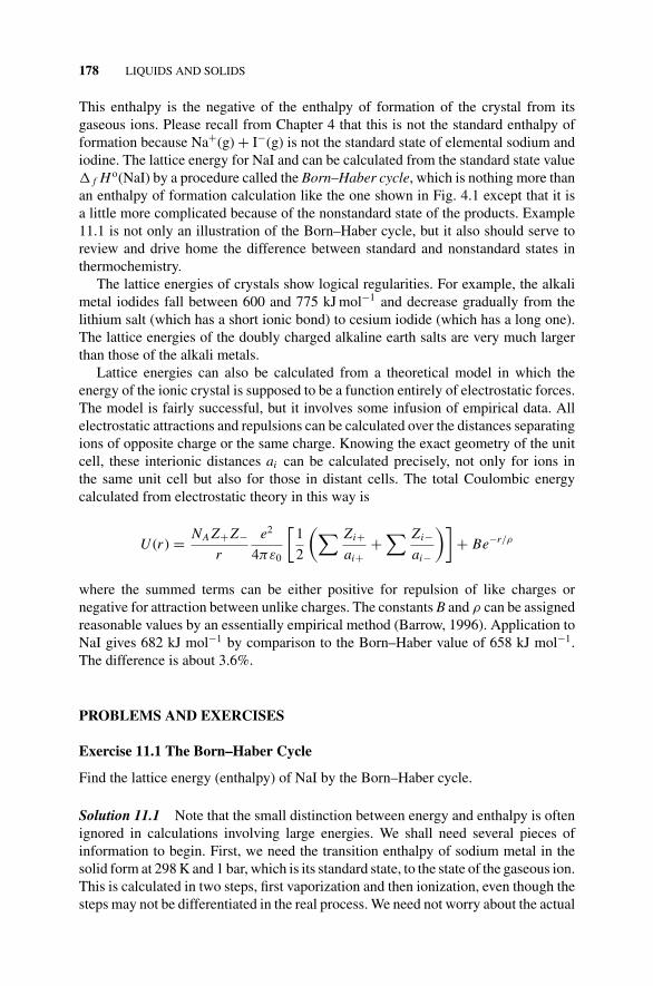
P1: OTA/XYZ P2: ABCc11 JWBS043-Rogers September 13, 2010 11:26 Printer Name: Yet to Come
178 LIQUIDS AND SOLIDS
This enthalpy is the negative of the enthalpy of formation of the crystal from itsgaseous ions. Please recall from Chapter 4 that this is not the standard enthalpy offormation because Na+(g) + I−(g) is not the standard state of elemental sodium andiodine. The lattice energy for NaI and can be calculated from the standard state value f H o(NaI) by a procedure called the Born–Haber cycle, which is nothing more thanan enthalpy of formation calculation like the one shown in Fig. 4.1 except that it isa little more complicated because of the nonstandard state of the products. Example11.1 is not only an illustration of the Born–Haber cycle, but it also should serve toreview and drive home the difference between standard and nonstandard states inthermochemistry.
The lattice energies of crystals show logical regularities. For example, the alkalimetal iodides fall between 600 and 775 kJ mol−1 and decrease gradually from thelithium salt (which has a short ionic bond) to cesium iodide (which has a long one).The lattice energies of the doubly charged alkaline earth salts are very much largerthan those of the alkali metals.
Lattice energies can also be calculated from a theoretical model in which theenergy of the ionic crystal is supposed to be a function entirely of electrostatic forces.The model is fairly successful, but it involves some infusion of empirical data. Allelectrostatic attractions and repulsions can be calculated over the distances separatingions of opposite charge or the same charge. Knowing the exact geometry of the unitcell, these interionic distances ai can be calculated precisely, not only for ions inthe same unit cell but also for those in distant cells. The total Coulombic energycalculated from electrostatic theory in this way is
U (r ) = NA Z+ Z−r
e2
4πε0
[1
2
(∑ Zi+ai+
+∑ Zi−
ai−
)]+ Be−r/ρ
where the summed terms can be either positive for repulsion of like charges ornegative for attraction between unlike charges. The constants B and ρ can be assignedreasonable values by an essentially empirical method (Barrow, 1996). Application toNaI gives 682 kJ mol−1 by comparison to the Born–Haber value of 658 kJ mol−1.The difference is about 3.6%.
PROBLEMS AND EXERCISES
Exercise 11.1 The Born–Haber Cycle
Find the lattice energy (enthalpy) of NaI by the Born–Haber cycle.
Solution 11.1 Note that the small distinction between energy and enthalpy is oftenignored in calculations involving large energies. We shall need several pieces ofinformation to begin. First, we need the transition enthalpy of sodium metal in thesolid form at 298 K and 1 bar, which is its standard state, to the state of the gaseous ion.This is calculated in two steps, first vaporization and then ionization, even though thesteps may not be differentiated in the real process. We need not worry about the actual
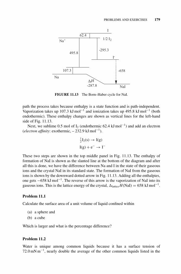
P1: OTA/XYZ P2: ABCc11 JWBS043-Rogers September 13, 2010 11:26 Printer Name: Yet to Come
PROBLEMS AND EXERCISES 179
107.3
495.8
Na
Na+ 1/2 I2
I
I-
NaI
∆fH
62.4
-295.3
-287.8
-658
FIGURE 11.13 The Born–Haber cycle for NaI.
path the process takes because enthalpy is a state function and is path-independent.Vaporization takes up 107.3 kJ mol−1 and ionization takes up 495.8 kJ mol−1 (bothendothermic). These enthalpy changes are shown as vertical lines for the left-handside of Fig. 11.13.
Next, we sublime 0.5 mol of I2 (endothermic 62.4 kJ mol−1) and add an electron(electron affinity: exothermic, – 232.9 kJ mol−1).
12 I2(s) → I(g)
I(g) + e− → I−
These two steps are shown in the top middle panel in Fig. 11.13. The enthalpy offormation of NaI is shown as the slanted line at the bottom of the diagram and afterall this is done, we have the difference between Na and I in the state of their gaseousions and the crystal NaI in its standard state. The formation of NaI from the gaseousions is shown by the downward dotted arrow in Fig. 11.13. Adding all the enthalpies,one gets −658 kJ mol−1. The reverse of this arrow is the vaporization of NaI into itsgaseous ions. This is the lattice energy of the crystal, lattice H (NaI) = 658 kJ mol−1.
Problem 11.1
Calculate the surface area of a unit volume of liquid confined within
(a) a sphere and
(b) a cube
Which is larger and what is the percentage difference?
Problem 11.2
Water is unique among common liquids because it has a surface tension of72.0 mN m−1, nearly double the average of the other common liquids listed in the
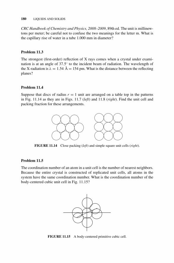
P1: OTA/XYZ P2: ABCc11 JWBS043-Rogers September 13, 2010 11:26 Printer Name: Yet to Come
180 LIQUIDS AND SOLIDS
CRC Handbook of Chemistry and Physics, 2008–2009, 89th ed. The unit is millinew-tons per meter; be careful not to confuse the two meanings for the letter m. What isthe capillary rise of water in a tube 1.000 mm in diameter?
Problem 11.3
The strongest (first-order) reflection of X rays comes when a crystal under exami-nation is at an angle of 37.5◦ to the incident beam of radiation. The wavelength ofthe X-radiation is λ = 1.54 A = 154 pm. What is the distance between the reflectingplanes?
Problem 11.4
Suppose that discs of radius r = 1 unit are arranged on a table top in the patternsin Fig. 11.14 as they are in Figs. 11.7 (left) and 11.8 (right). Find the unit cell andpacking fraction for these arrangements.
FIGURE 11.14 Close packing (left) and simple square unit cells (right).
Problem 11.5
The coordination number of an atom in a unit cell is the number of nearest neighbors.Because the entire crystal is constructed of replicated unit cells, all atoms in thesystem have the same coordination number. What is the coordination number of thebody-centered cubic unit cell in Fig. 11.15?
FIGURE 11.15 A body-centered primitive cubic cell.
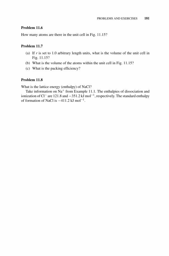
P1: OTA/XYZ P2: ABCc11 JWBS043-Rogers September 13, 2010 11:26 Printer Name: Yet to Come
PROBLEMS AND EXERCISES 181
Problem 11.6
How many atoms are there in the unit cell in Fig. 11.15?
Problem 11.7
(a) If r is set to 1.0 arbitrary length units, what is the volume of the unit cell inFig. 11.15?
(b) What is the volume of the atoms within the unit cell in Fig. 11.15?
(c) What is the packing efficiency?
Problem 11.8
What is the lattice energy (enthalpy) of NaCl?Take information on Na+ from Example 11.1. The enthalpies of dissociation and
ionization of Cl− are 121.8 and −351.2 kJ mol−1, respectively. The standard enthalpyof formation of NaCl is −411.2 kJ mol−1.
P1: OTA/XYZ P2: ABCc12 JWBS043-Rogers September 13, 2010 11:27 Printer Name: Yet to Come
12SOLUTION CHEMISTRY
The concept of the ideal solution is as useful as the concept of the ideal gas, but thereference states must be very different because a model having no intermolecularinteractions would not be a liquid. The next best thing is to propose a model in whichno change in molecular forces takes place upon mixing two completely miscibleliquids. In this model, mixing of two ideal liquids would be essentially the same asmixing of two ideal gases (Section 5.3.1). The enthalpy change would be zero at allproportions, and the mixing process would be entirely driven by a positive entropychange.
12.1 THE IDEAL SOLUTION
The enthalpy of mixing to form an ideal solution
A(pure) + B(pure) → AB(mixed)
is zero because no change takes place in attractive forces upon going from isolatedA and isolated B to AB neighbors in the mixture. On the other hand, the entropyof a system of two pure isolated liquids A and B, in which an observer knows thatany randomly selected molecule will be either A or B according to which “beaker”it is drawn from, is replaced by a mixed system of greater disorder where random
Concise Physical Chemistry, by Donald W. RogersCopyright C© 2011 John Wiley & Sons, Inc.
182
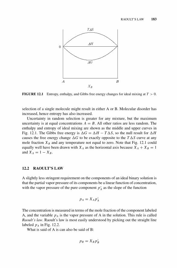
P1: OTA/XYZ P2: ABCc12 JWBS043-Rogers September 13, 2010 11:27 Printer Name: Yet to Come
RAOULT’S LAW 183
0
TΔS
ΔH
ΔG
Α Β XB
FIGURE 12.1 Entropy, enthalpy, and Gibbs free energy changes for ideal mixing at T > 0.
selection of a single molecule might result in either A or B. Molecular disorder hasincreased, hence entropy has also increased.
Uncertainty in random selection is greater for any mixture, but the maximumuncertainty is at equal concentrations A = B. All other ratios are less random. Theenthalpy and entropy of ideal mixing are shown as the middle and upper curves inFig. 12.1. The Gibbs free energy is �G = �H − T �S, so the null result for �Hcauses the free energy change �G to be exactly opposite to the T �S curve at anymole fraction X B and any temperature not equal to zero. Note that Fig. 12.1 couldequally well have been drawn with X A as the horizontal axis because X A + X B = 1and X A = 1 − X B .
12.2 RAOULT’S LAW
A slightly less stringent requirement on the components of an ideal binary solution isthat the partial vapor pressure of its components be a linear function of concentration,with the vapor pressure of the pure component p◦
A as the slope of the function
pA = X A p◦A
The concentration is measured in terms of the mole fraction of the component labeledA, and the variable pA is the vapor pressure of A in the solution. This rule is calledRaoult’s law. Raoult’s law is most easily understood by picking out the straight linelabeled pA in Fig. 12.2.
What is said of A is can also be said of B:
pB = X B p◦B
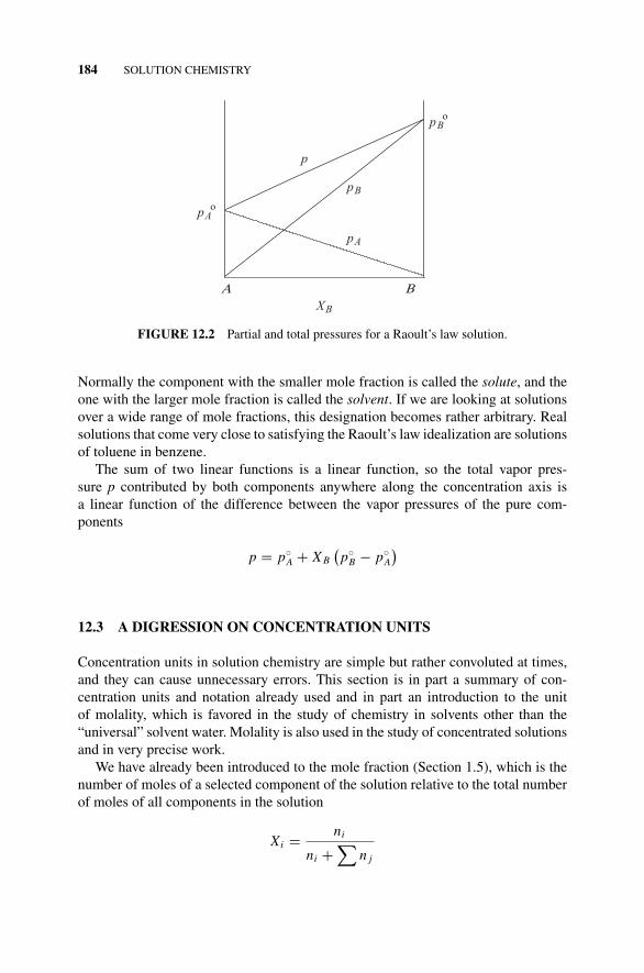
P1: OTA/XYZ P2: ABCc12 JWBS043-Rogers September 13, 2010 11:27 Printer Name: Yet to Come
184 SOLUTION CHEMISTRY
Α Β XB
p
pB
pA
pBo
pAo
FIGURE 12.2 Partial and total pressures for a Raoult’s law solution.
Normally the component with the smaller mole fraction is called the solute, and theone with the larger mole fraction is called the solvent. If we are looking at solutionsover a wide range of mole fractions, this designation becomes rather arbitrary. Realsolutions that come very close to satisfying the Raoult’s law idealization are solutionsof toluene in benzene.
The sum of two linear functions is a linear function, so the total vapor pres-sure p contributed by both components anywhere along the concentration axis isa linear function of the difference between the vapor pressures of the pure com-ponents
p = p◦A + X B
(p◦
B − p◦A
)
12.3 A DIGRESSION ON CONCENTRATION UNITS
Concentration units in solution chemistry are simple but rather convoluted at times,and they can cause unnecessary errors. This section is in part a summary of con-centration units and notation already used and in part an introduction to the unitof molality, which is favored in the study of chemistry in solvents other than the“universal” solvent water. Molality is also used in the study of concentrated solutionsand in very precise work.
We have already been introduced to the mole fraction (Section 1.5), which is thenumber of moles of a selected component of the solution relative to the total numberof moles of all components in the solution
Xi = ni
ni +∑
n j
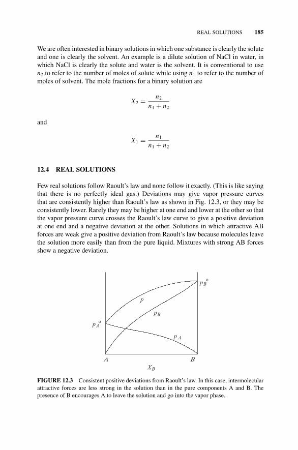
P1: OTA/XYZ P2: ABCc12 JWBS043-Rogers September 13, 2010 11:27 Printer Name: Yet to Come
REAL SOLUTIONS 185
We are often interested in binary solutions in which one substance is clearly the soluteand one is clearly the solvent. An example is a dilute solution of NaCl in water, inwhich NaCl is clearly the solute and water is the solvent. It is conventional to usen2 to refer to the number of moles of solute while using n1 to refer to the number ofmoles of solvent. The mole fractions for a binary solution are
X2 = n2
n1 + n2
and
X1 = n1
n1 + n2
12.4 REAL SOLUTIONS
Few real solutions follow Raoult’s law and none follow it exactly. (This is like sayingthat there is no perfectly ideal gas.) Deviations may give vapor pressure curvesthat are consistently higher than Raoult’s law as shown in Fig. 12.3, or they may beconsistently lower. Rarely they may be higher at one end and lower at the other so thatthe vapor pressure curve crosses the Raoult’s law curve to give a positive deviationat one end and a negative deviation at the other. Solutions in which attractive ABforces are weak give a positive deviation from Raoult’s law because molecules leavethe solution more easily than from the pure liquid. Mixtures with strong AB forcesshow a negative deviation.
Α Β XB
p
pB
p A
pBo
pAo
FIGURE 12.3 Consistent positive deviations from Raoult’s law. In this case, intermolecularattractive forces are less strong in the solution than in the pure components A and B. Thepresence of B encourages A to leave the solution and go into the vapor phase.

P1: OTA/XYZ P2: ABCc12 JWBS043-Rogers September 13, 2010 11:27 Printer Name: Yet to Come
186 SOLUTION CHEMISTRY
12.5 HENRY’S LAW
The shape of the pB curve in Fig. 12.3 suggests another model similar to Raoult’slaw but with a different slope for the lower (solute) end of the curve. According toHenry’s law, the partial pressure, is the linear function found at the limit of infinitelydilute solutions (in practice, very dilute solutions). Like the ideal gas law, it is alimiting law (Rosenberg and Peticolas, 2004).
At relatively high concentrations of solute B, Henry’s law is a poor approximationbut it is clear from Fig. 12.4 that in the very dilute region near the vertical marker,it is a better descriptor of the partial vapor pressure of B than Raoult’s law. On thecontrary, at X B → 1 (toward the right in Fig. 12.4), B follows Raoult’s law. Now wehave a combined model: Raoult’s law for B acting as a solvent in high concentrationsand Henry’s law for B acting as a solute in low concentrations.
12.5.1 Henry’s Law Activities
We have encountered activities and activity coefficients before. A Henry’s law activityof solute B in solvent A is shown as a vertical line well to the left on the X B axis ofFig. 12.4, where X B is small. The activity coefficient γ is the ratio of real pB to theideal, as determined by Henry’s law. For the behavior of B shown in Fig. 12.4, theactivity coefficient will be γ < 1 in all cases because real behavior is always less thanideal. It will approach γ = 1 in the limit of infinite dilution. If the partial pressurecurve in Fig. 12.4 were below the Raoult’s law dotted line, all Henry’s law activitycoefficients would be γ > 1.
The model we have described so far is for binary solutions in which the componentsare mutually miscible (soluble in each other in all proportions). Everything we have
Α Β XB
pB
pBo
FIGURE 12.4 Henry’s law for the partial pressure of component B as the solute. The solidline is a Henry’s law extrapolation to infinite dilution of B. The dotted line is Raoult’s law.
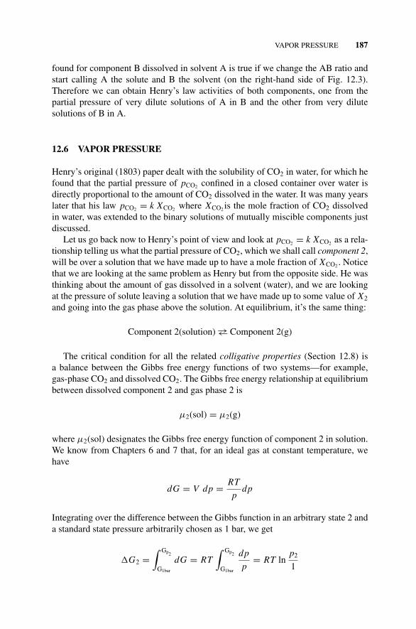
P1: OTA/XYZ P2: ABCc12 JWBS043-Rogers September 13, 2010 11:27 Printer Name: Yet to Come
VAPOR PRESSURE 187
found for component B dissolved in solvent A is true if we change the AB ratio andstart calling A the solute and B the solvent (on the right-hand side of Fig. 12.3).Therefore we can obtain Henry’s law activities of both components, one from thepartial pressure of very dilute solutions of A in B and the other from very dilutesolutions of B in A.
12.6 VAPOR PRESSURE
Henry’s original (1803) paper dealt with the solubility of CO2 in water, for which hefound that the partial pressure of pCO2 confined in a closed container over water isdirectly proportional to the amount of CO2 dissolved in the water. It was many yearslater that his law pCO2 = k XCO2 where XCO2 is the mole fraction of CO2 dissolvedin water, was extended to the binary solutions of mutually miscible components justdiscussed.
Let us go back now to Henry’s point of view and look at pCO2 = k XCO2 as a rela-tionship telling us what the partial pressure of CO2, which we shall call component 2,will be over a solution that we have made up to have a mole fraction of XCO2 . Noticethat we are looking at the same problem as Henry but from the opposite side. He wasthinking about the amount of gas dissolved in a solvent (water), and we are lookingat the pressure of solute leaving a solution that we have made up to some value of X2
and going into the gas phase above the solution. At equilibrium, it’s the same thing:
Component 2(solution) →← Component 2(g)
The critical condition for all the related colligative properties (Section 12.8) isa balance between the Gibbs free energy functions of two systems—for example,gas-phase CO2 and dissolved CO2. The Gibbs free energy relationship at equilibriumbetween dissolved component 2 and gas phase 2 is
µ2(sol) = µ2(g)
where µ2(sol) designates the Gibbs free energy function of component 2 in solution.We know from Chapters 6 and 7 that, for an ideal gas at constant temperature, wehave
dG = V dp = RT
pdp
Integrating over the difference between the Gibbs function in an arbitrary state 2 anda standard state pressure arbitrarily chosen as 1 bar, we get
�G2 =∫ Gp2
G1bar
dG = RT∫ Gp2
G1bar
dp
p= RT ln
p2
1
P1: OTA/XYZ P2: ABCc12 JWBS043-Rogers September 13, 2010 11:27 Printer Name: Yet to Come
188 SOLUTION CHEMISTRY
Written in terms of Gibbs chemical potentials, this gives us
µ2(g) = µ◦2(g) + RT ln
p2
p◦ = µ◦2(g) + RT ln p2
where µ◦2(g) is the standard state free energy for an ideal gas at a partial pressure p2
in a mixture of gases. The analogous expression for an ideal solute at mole fractionX2 in a mixture of solutes is
µ2(sol) = µ◦2(sol) + RT ln X2
(We shall usually treat the special case of only one solute dissolved in one solvent.)Equality of the two Gibbs potentials at equilibrium gives
µ2(sol) = µ2(g)
µ◦2(g) + RT ln p2 = µ◦
2(sol) + RT ln X2
or
RT lnp2
X2= µ◦
2(sol) − µ◦2(g)
This leads to an expression with only constants on the right-hand side:
lnp2
X2= µ◦
2(sol) − µ◦2(g)
RT
or
p2
X2= e
µ◦2(sol)−µ◦
2(g)
RT = econst = k
which is Henry’s law, p2 = k X2. Notice that the difference between Raoult’s lawand Henry’s law is merely in the arbitrary selection of a standard state.
12.7 BOILING POINT ELEVATION
The utility of Henry’s law becomes apparent when we consider a very importantclass of binary solutions, the class of nonvolatile solutes in a volatile solvent—forexample, sugar (sucrose) in water. The nonvolatile solute has no measurable vaporpressure, hence Raoult’s law does not apply because there is no p◦
B in Figs. 12.3 and12.4. The total vapor pressure is due to the solvent:
p = X1 p◦1

P1: OTA/XYZ P2: ABCc12 JWBS043-Rogers September 13, 2010 11:27 Printer Name: Yet to Come
BOILING POINT ELEVATION 189
p
T
1 atm
Tb
p
T
Δp
ΔTb
FIGURE 12.5 Boiling of pure solvent (left) and a solution of solvent and nonvolatile solute(right). The temperature of the solution must be increased by �Tb to restore its vapor pressureto 1 atm.
Addition of a nonvolatile solute causes a change in the vapor pressure of the solutionaccording to the amount of solute added because (1 − X1) = X2 for a binary solution:
�p = p◦1 − p = p◦
1 − X1 p◦1 = p◦
1(1 − X1) = p◦1 X2
The statement �p = p◦1 X2 is true only in the limit of very dilute solutions.
To see that addition of a small amount of nonvolatile solute causes an elevation ofthe boiling point of the solution relative to the pure solvent, consider a solvent thathas an exponential variation of p with T as in Fig. 12.5 (left). Its boiling point is thetemperature at which the vapor pressure is equal to the pressure of the atmospherebearing down on the surface of the liquid (dotted line).
When a nonvolatile solute is added to the solvent, its entire vapor pressure curveis displaced downward by �p. An increase in temperature is necessary to restore thevapor pressure to 1 atm. The vapor pressure of the solution moves along the lowerexponential curve with increasing temperature until it arrives once again at 1 atm and�Tb, whereupon boiling recommences. It is evident that a functional relationshipmust exist among �p, X2, and �Tb. To find the relation between the amount ofnonvolatile solute and �Tb we have recourse to the Clausius–Clapeyron equation
ln p = −�vap H
R
(1
T
)+ const
Differentiating, we obtain
d ln p = dp
p= �vap H
R
(1
T 2
)dT
If we take dp/p as �p/p for a very small but finite and measurable �p, broughtabout by addition of the solute, we must increase the temperature by an amount
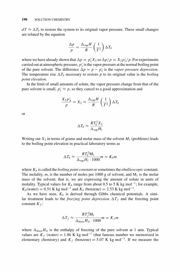
P1: OTA/XYZ P2: ABCc12 JWBS043-Rogers September 13, 2010 11:27 Printer Name: Yet to Come
190 SOLUTION CHEMISTRY
dT ≈ �Tb to restore the system to its original vapor pressure. These small changesare related by the equation
�p
p= �vap H
R
(1
T 2
)�Tb
where we have already shown that �p = p◦1 X2 so �p/p = X2 p◦
1/p. For experimentscarried out at atmospheric pressure, p◦
1 is the vapor pressure at the normal boiling pointof the pure solvent. The difference �p = p − p◦
1 is the vapor pressure depression.The temperature rise �Tb necessary to restore p to its original value is the boilingpoint elevation.
In the limit of small amounts of solute, the vapor pressure change from that of thepure solvent is small, p◦
1 ≈ p, so they cancel to a good approximation and
X2 p◦A
p≈ X2 ≈ �vap H
R
(1
T 2
)�Tb
or
�Tb ≈ RT 2b X2
�vap H1
Writing out X2 in terms of grams and molar mass of the solvent M1 (problems) leadsto the boiling point elevation in practical laboratory terms as
�Tb ≈ RT 2b M1
�vap H1 · 1000m = Kbm
where Kb is called the boiling point constant or sometimes the ebullioscopic constant.The molality, m, is the number of moles per 1000 g of solvent, and M1 is the molarmass of the solvent; that is, we are expressing the amount of solute in units ofmolality. Typical values for Kb range from about 0.5 to 5 K kg mol−1; for example,Kb(water) = 0.51 K kg mol−1 and Kb (benzene) = 2.53 K kg mol−1.
As we have seen, Kb is derived through Gibbs chemical potentials. A simi-lar treatment leads to the freezing point depression �T f and the freezing pointconstant K f :
�T f ≈ RT 2f M1
�freez HA · 1000m = K f m
where �freez HA is the enthalpy of freezing of the pure solvent at 1 atm. Typicalvalues are K f (water) = 1.86 K kg mol−1 (that famous number we memorized inelementary chemistry) and K f (benzene) = 5.07 K kg mol−1. If we measure the

P1: OTA/XYZ P2: ABCc12 JWBS043-Rogers September 13, 2010 11:27 Printer Name: Yet to Come
OSMOTIC PRESURE 191
freezing point depression brought about by dissolution of a known (small) weight ofsolute to produce a dilute solution, we can calculate the number of moles of solutefrom �T f , hence its molar mass in units of kg mol−1.
12.8 OSMOTIC PRESURE
Many membranes have the property that they pass small molecules but not largeones. They are semipermeable. The human kidney contains semipermeable mem-branes that separate salt and urea from the bloodstream for excretion but do not passblood protein. If a semipermeable membrane separates two arms of a U tube and asolution of a protein is placed in one arm of the tube with the solvent in the otherarm, solvent molecules will pass through the membrane into the protein solutionbecause of the spontaneous tendency of the protein solution to evolve toward a moredilute state of higher entropy. The process is called osmosis. The liquid level in theprotein arm of the U tube will rise until the downward pressure it exerts on themembrane due to gravity is just sufficient to balance the entropy-driven osmotic flowacross the membrane. This osmotic pressure, π , follows a law similar to the idealgas law:
πV = n RT
where V is the volume of a solution containing n moles of the macromolecularsolute.
We have already made the point that liquids, contrary to gases, are subject to strongintermolecular interactions. The internal structure of the liquid state is distinct anddifferent from that of the gaseous state, so why should a property of solutions followwhat appears to be an ideal gas law? The derivation of the osmotic law to arrive atthis remarkable and somewhat counterintuitive conclusion is quite distinct from idealgas law theory, and it reveals some of the power of the condition that, at equilibrium,the Gibbs chemical potential must be the same over different macroscopic segmentsof the same thermodynamic system.
To apply this idea to a real system, we find the osmotic pressure on the solutionin the right-hand chamber of Fig. 12.6 by a two-step process. First we shall calculatethe total pressure, which is the ambient pressure p plus an arbitrary pressure π onpure solvent, through our knowledge of the variation of the Gibbs chemical potentialwith variation in pressure. Second we shall find the variation of the Gibbs chemicalpotential brought about by addition of a small amount of solute. These two steps arethen summed to find the total pressure on the solution of solvent plus solute.
Step 1
Start with pure solvent and apply some pressure π at constant temperature. TheGibbs free energy of the system is the Gibbs free energy of the pure solvent at
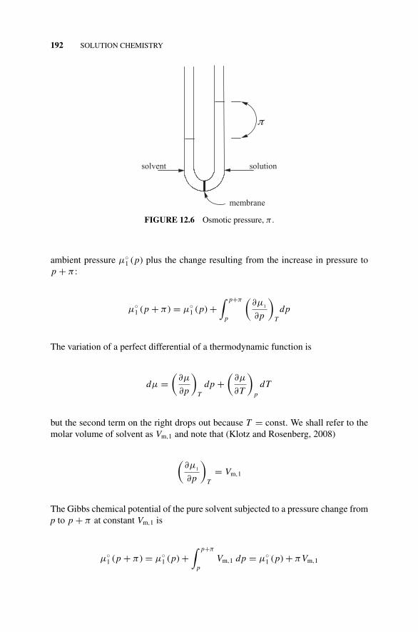
P1: OTA/XYZ P2: ABCc12 JWBS043-Rogers September 13, 2010 11:27 Printer Name: Yet to Come
192 SOLUTION CHEMISTRY
π
solvent solution
membrane
FIGURE 12.6 Osmotic pressure, π .
ambient pressure µ◦1 (p) plus the change resulting from the increase in pressure to
p + π :
µ◦1 (p + π ) = µ◦
1 (p) +∫ p+π
p
(∂µ1
∂p
)T
dp
The variation of a perfect differential of a thermodynamic function is
dµ =(
∂µ
∂p
)T
dp +(
∂µ
∂T
)p
dT
but the second term on the right drops out because T = const. We shall refer to themolar volume of solvent as Vm,1 and note that (Klotz and Rosenberg, 2008)
(∂µ1
∂p
)T
= Vm,1
The Gibbs chemical potential of the pure solvent subjected to a pressure change fromp to p + π at constant Vm,1 is
µ◦1 (p + π ) = µ◦
1 (p) +∫ p+π
pVm,1 dp = µ◦
1 (p) + πVm,1
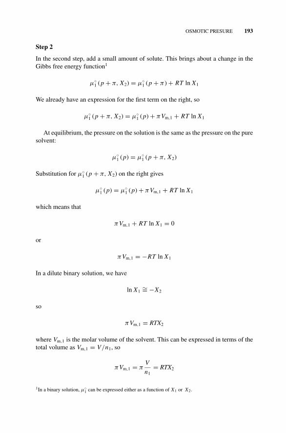
P1: OTA/XYZ P2: ABCc12 JWBS043-Rogers September 13, 2010 11:27 Printer Name: Yet to Come
OSMOTIC PRESURE 193
Step 2
In the second step, add a small amount of solute. This brings about a change in theGibbs free energy function1
µ◦1 (p + π, X2) = µ◦
1 (p + π ) + RT ln X1
We already have an expression for the first term on the right, so
µ◦1 (p + π, X2) = µ◦
1 (p) + πVm,1 + RT ln X1
At equilibrium, the pressure on the solution is the same as the pressure on the puresolvent:
µ◦1 (p) = µ◦
1 (p + π, X2)
Substitution for µ◦1 (p + π, X2) on the right gives
µ◦1 (p) = µ◦
1 (p) + πVm,1 + RT ln X1
which means that
πVm,1 + RT ln X1 = 0
or
πVm,1 = −RT ln X1
In a dilute binary solution, we have
ln X1∼= −X2
so
πVm,1 = RTX2
where Vm,1 is the molar volume of the solvent. This can be expressed in terms of thetotal volume as Vm,1 = V/n1, so
πVm,1 = πV
n1= RTX2
1In a binary solution, µ◦1 can be expressed either as a function of X1 or X2.
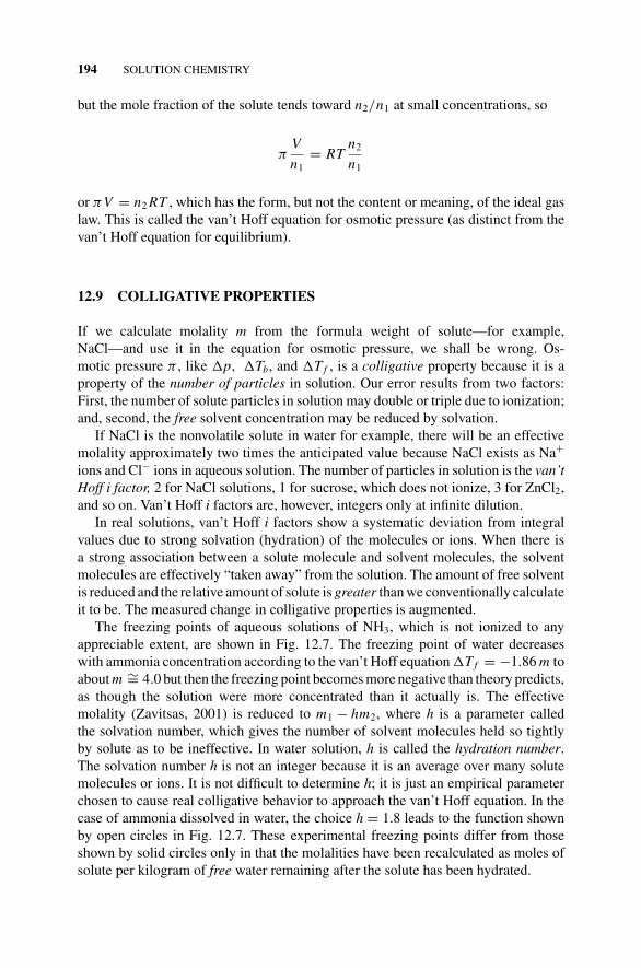
P1: OTA/XYZ P2: ABCc12 JWBS043-Rogers September 13, 2010 11:27 Printer Name: Yet to Come
194 SOLUTION CHEMISTRY
but the mole fraction of the solute tends toward n2/n1 at small concentrations, so
πV
n1= RT
n2
n1
or πV = n2 RT , which has the form, but not the content or meaning, of the ideal gaslaw. This is called the van’t Hoff equation for osmotic pressure (as distinct from thevan’t Hoff equation for equilibrium).
12.9 COLLIGATIVE PROPERTIES
If we calculate molality m from the formula weight of solute—for example,NaCl—and use it in the equation for osmotic pressure, we shall be wrong. Os-motic pressure π , like �p, �Tb, and �T f , is a colligative property because it is aproperty of the number of particles in solution. Our error results from two factors:First, the number of solute particles in solution may double or triple due to ionization;and, second, the free solvent concentration may be reduced by solvation.
If NaCl is the nonvolatile solute in water for example, there will be an effectivemolality approximately two times the anticipated value because NaCl exists as Na+
ions and Cl− ions in aqueous solution. The number of particles in solution is the van’tHoff i factor, 2 for NaCl solutions, 1 for sucrose, which does not ionize, 3 for ZnCl2,and so on. Van’t Hoff i factors are, however, integers only at infinite dilution.
In real solutions, van’t Hoff i factors show a systematic deviation from integralvalues due to strong solvation (hydration) of the molecules or ions. When there isa strong association between a solute molecule and solvent molecules, the solventmolecules are effectively “taken away” from the solution. The amount of free solventis reduced and the relative amount of solute is greater than we conventionally calculateit to be. The measured change in colligative properties is augmented.
The freezing points of aqueous solutions of NH3, which is not ionized to anyappreciable extent, are shown in Fig. 12.7. The freezing point of water decreaseswith ammonia concentration according to the van’t Hoff equation �T f = −1.86 m toabout m ∼= 4.0 but then the freezing point becomes more negative than theory predicts,as though the solution were more concentrated than it actually is. The effectivemolality (Zavitsas, 2001) is reduced to m1 − hm2, where h is a parameter calledthe solvation number, which gives the number of solvent molecules held so tightlyby solute as to be ineffective. In water solution, h is called the hydration number.The solvation number h is not an integer because it is an average over many solutemolecules or ions. It is not difficult to determine h; it is just an empirical parameterchosen to cause real colligative behavior to approach the van’t Hoff equation. In thecase of ammonia dissolved in water, the choice h = 1.8 leads to the function shownby open circles in Fig. 12.7. These experimental freezing points differ from thoseshown by solid circles only in that the molalities have been recalculated as moles ofsolute per kilogram of free water remaining after the solute has been hydrated.
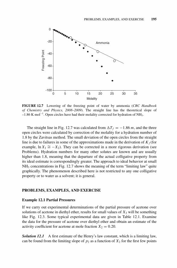
P1: OTA/XYZ P2: ABCc12 JWBS043-Rogers September 13, 2010 11:27 Printer Name: Yet to Come
PROBLEMS, EXAMPLES, AND EXERCISE 195
Ammonia
Molality
35302520151050
Fre
ezin
g P
oint
-100
-80
-60
-40
-20
0
FIGURE 12.7 Lowering of the freezing point of water by ammonia (CRC Handbookof Chemistry and Physics, 2008–2009). The straight line has the theoretical slope of–1.86 K mol−1. Open circles have had their molality corrected for hydration of NH3.
The straight line in Fig. 12.7 was calculated from �T f = −1.86 m, and the threeopen circles were calculated by correction of the molality for a hydration number of1.8 by the Zavitsas method. The small deviation of the open circles from the straightline is due to failures in some of the approximations made in the derivation of K f (forexample, ln X1
∼= −X2). They can be corrected in a more rigorous derivation (seeProblems). Hydration numbers for many other solutes are known and are usuallyhigher than 1.8, meaning that the departure of the actual colligative property fromits ideal estimate is correspondingly greater. The approach to ideal behavior at smallNH3 concentrations in Fig. 12.7 shows the meaning of the term “limiting law” quitegraphically. The phenomenon described here is not restricted to any one colligativeproperty or to water as a solvent; it is general.
PROBLEMS, EXAMPLES, AND EXERCISE
Example 12.1 Partial Pressures
If we carry out experimental determinations of the partial pressure of acetone oversolutions of acetone in diethyl ether, results for small values of X2 will be somethinglike Fig. 12.3. Some typical experimental data are given in Table 12.1. Examinethe data for the pressure of acetone over diethyl ether and obtain an estimate of theactivity coefficient for acetone at mole fraction X2 = 0.20.
Solution 12.1 A first estimate of the Henry’s law constant, which is a limiting law,can be found from the limiting slope of p2 as a function of X2 for the first few points
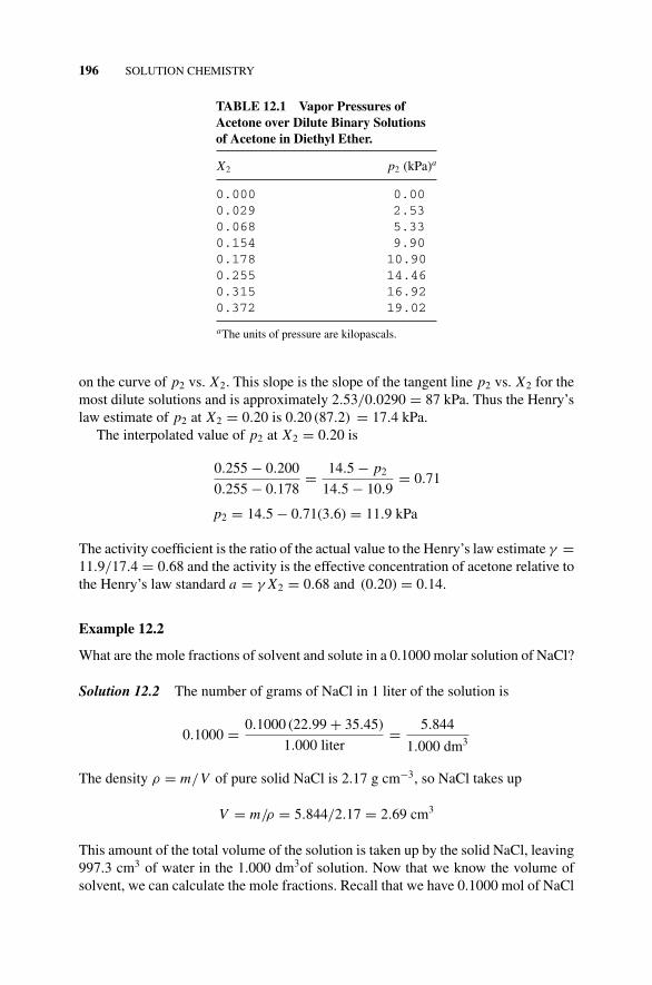
P1: OTA/XYZ P2: ABCc12 JWBS043-Rogers September 13, 2010 11:27 Printer Name: Yet to Come
196 SOLUTION CHEMISTRY
TABLE 12.1 Vapor Pressures ofAcetone over Dilute Binary Solutionsof Acetone in Diethyl Ether.
X2 p2 (kPa)a
0.000 0.000.029 2.530.068 5.330.154 9.900.178 10.900.255 14.460.315 16.920.372 19.02
aThe units of pressure are kilopascals.
on the curve of p2 vs. X2. This slope is the slope of the tangent line p2 vs. X2 for themost dilute solutions and is approximately 2.53/0.0290 = 87 kPa. Thus the Henry’slaw estimate of p2 at X2 = 0.20 is 0.20 (87.2) = 17.4 kPa.
The interpolated value of p2 at X2 = 0.20 is
0.255 − 0.200
0.255 − 0.178= 14.5 − p2
14.5 − 10.9= 0.71
p2 = 14.5 − 0.71(3.6) = 11.9 kPa
The activity coefficient is the ratio of the actual value to the Henry’s law estimate γ =11.9/17.4 = 0.68 and the activity is the effective concentration of acetone relative tothe Henry’s law standard a = γ X2 = 0.68 and (0.20) = 0.14.
Example 12.2
What are the mole fractions of solvent and solute in a 0.1000 molar solution of NaCl?
Solution 12.2 The number of grams of NaCl in 1 liter of the solution is
0.1000 = 0.1000 (22.99 + 35.45)
1.000 liter= 5.844
1.000 dm3
The density ρ = m/V of pure solid NaCl is 2.17 g cm−3, so NaCl takes up
V = m/ρ = 5.844/2.17 = 2.69 cm3
This amount of the total volume of the solution is taken up by the solid NaCl, leaving997.3 cm3 of water in the 1.000 dm3of solution. Now that we know the volume ofsolvent, we can calculate the mole fractions. Recall that we have 0.1000 mol of NaCl

P1: OTA/XYZ P2: ABCc12 JWBS043-Rogers September 13, 2010 11:27 Printer Name: Yet to Come
PROBLEMS, EXAMPLES, AND EXERCISE 197
by definition and the molar mass of water is 18.02, so we have 997.3/18.02 = 55.345mol of water. The mole fractions are
X2 = n2
n1 + n2= 0.1000
55.345 + 0.1000= 1.804 × 10−3
and
X1 = n1
n1 + n2= 55.345
55.345 + 0.1000= 0.9982
Comment: First, notice that the sum of the two mole fractions is exactly 1.000, asit should be because there are only two components in this solution. Second, noticethat we have already made some pretty serious approximations and assumptions. Wedon’t really have the right to assume that the volume taken up by NaCl in solutionis the same as the volume in the crystalline state. Also we are assuming that thedensity of water is exactly 1.000 kg dm−3 and the volume of the solution is exactly1.000 dm3 without specifying the temperature. We shall have to take these approxi-mations more seriously later.
In precise solution chemistry, we often use molal concentrations, the amount ofsolute expressed in moles per 1000 g of solvent in contrast to the ordinary stockroomunit of moles per liter or molarity. A 0.1000 molal solution contains 1000/18.02 =55.494 moles of water, but so does a 0.2000 molal solution because the volume ofthe solute is not subtracted from that of the solvent. That is one advantage of themolal convention. Another is that the number of grams in a molal solution doesnot depend on the temperature, but the number of grams in a molar solution doesbecause the volume of the solution is temperature-dependent. The mole fraction of the0.1000 molal solution is
X2 = n2
n1 + n2= 0.1000
55.494 + 0.1000= 1.800 × 10−3
and
X1 = n1
n1 + n2= 55.494
55.494 + 0.1000= 0.9982
with a sum of 1.000 as before.Why specify a new concentration unit when it comes out the same as the old
one? As the following exercise shows, it does not come out exactly the same andsometimes it is not even close. For very dilute solutions, the difference is negligible,which is why the concentrations of solutions in working labs and elementary coursesare usually given in molarity rather than molality. In medicinal and clinical chemistry,many other concentration units are used but they can all be reduced to the basic oneswith a little algebra.
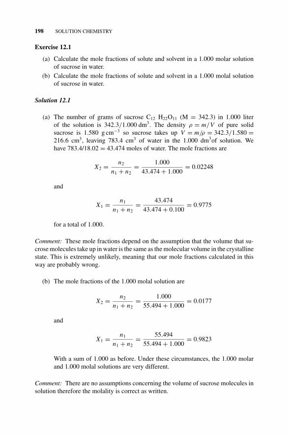
P1: OTA/XYZ P2: ABCc12 JWBS043-Rogers September 13, 2010 11:27 Printer Name: Yet to Come
198 SOLUTION CHEMISTRY
Exercise 12.1
(a) Calculate the mole fractions of solute and solvent in a 1.000 molar solutionof sucrose in water.
(b) Calculate the mole fractions of solute and solvent in a 1.000 molal solutionof sucrose in water.
Solution 12.1
(a) The number of grams of sucrose C12 H22O11 (M = 342.3) in 1.000 literof the solution is 342.3/1.000 dm3. The density ρ = m/V of pure solidsucrose is 1.580 g cm−3 so sucrose takes up V = m/ρ = 342.3/1.580 =216.6 cm3, leaving 783.4 cm3 of water in the 1.000 dm3of solution. Wehave 783.4/18.02 = 43.474 moles of water. The mole fractions are
X2 = n2
n1 + n2= 1.000
43.474 + 1.000= 0.02248
and
X1 = n1
n1 + n2= 43.474
43.474 + 0.100= 0.9775
for a total of 1.000.
Comment: These mole fractions depend on the assumption that the volume that su-crose molecules take up in water is the same as the molecular volume in the crystallinestate. This is extremely unlikely, meaning that our mole fractions calculated in thisway are probably wrong.
(b) The mole fractions of the 1.000 molal solution are
X2 = n2
n1 + n2= 1.000
55.494 + 1.000= 0.0177
and
X1 = n1
n1 + n2= 55.494
55.494 + 1.000= 0.9823
With a sum of 1.000 as before. Under these circumstances, the 1.000 molarand 1.000 molal solutions are very different.
Comment: There are no assumptions concerning the volume of sucrose molecules insolution therefore the molality is correct as written.
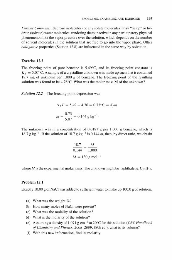
P1: OTA/XYZ P2: ABCc12 JWBS043-Rogers September 13, 2010 11:27 Printer Name: Yet to Come
PROBLEMS, EXAMPLES, AND EXERCISE 199
Further Comment: Sucrose molecules (or any solute molecules) may “tie up” or hy-drate (solvate) water molecules, rendering them inactive in any participatory physicalphenomenon like the vapor pressure over the solution, which depends on the numberof solvent molecules in the solution that are free to go into the vapor phase. Othercolligative properties (Section 12.8) are influenced in the same way by solvation.
Exercise 12.2
The freezing point of pure benzene is 5.49◦C, and its freezing point constant isK f = 5.07◦C. A sample of a crystalline unknown was made up such that it contained18.7 mg of unknown per 1.000 g of benzene. The freezing point of the resultingsolution was found to be 4.76◦C. What was the molar mass M of the unknown?
Solution 12.2 The freezing point depression was
� f T = 5.49 − 4.76 = 0.73◦C = Kf m
m = 0.73
5.07= 0.144 g kg−1
The unknown was in a concentration of 0.0187 g per 1.000 g benzene, which is18.7 g kg−1. If the solution of 18.7 g kg−1 is 0.144 m, then, by direct ratio, we obtain
18.7
0.144= M
1.000
M = 130 g mol−1
where M is the experimental molar mass. The unknown might be naphthalene, C10H10.
Problem 12.1
Exactly 10.00 g of NaCl was added to sufficient water to make up 100.0 g of solution.
(a) What was the weight %?
(b) How many moles of NaCl were present?
(c) What was the molality of the solution?
(d) What is the molarity of the solution?
(e) Assuming a density of 1.071 g cm−3 at 20◦C for this solution (CRC Handbookof Chemistry and Physics, 2008–2009, 89th ed.), what is its volume?
(f) With this new information, find its molarity.
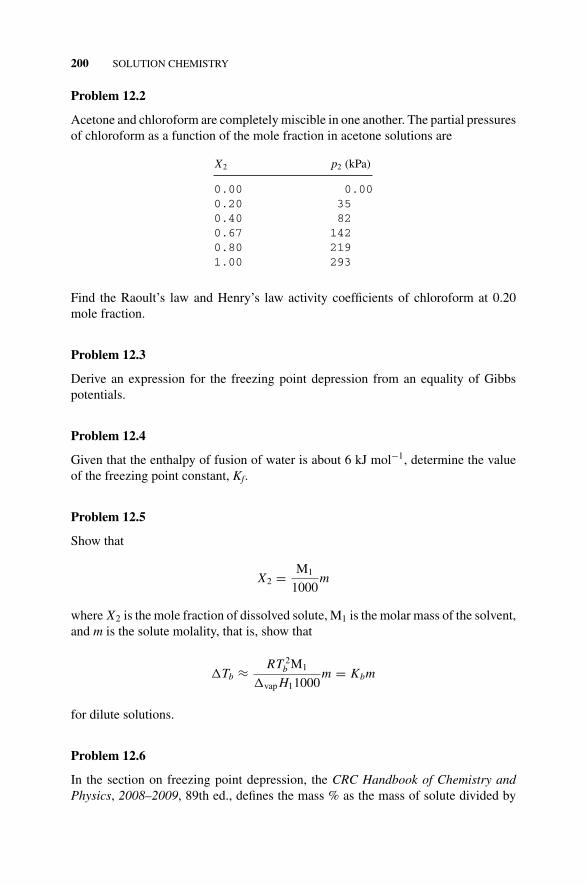
P1: OTA/XYZ P2: ABCc12 JWBS043-Rogers September 13, 2010 11:27 Printer Name: Yet to Come
200 SOLUTION CHEMISTRY
Problem 12.2
Acetone and chloroform are completely miscible in one another. The partial pressuresof chloroform as a function of the mole fraction in acetone solutions are
X2 p2 (kPa)
0.00 0.000.20 350.40 820.67 1420.80 2191.00 293
Find the Raoult’s law and Henry’s law activity coefficients of chloroform at 0.20mole fraction.
Problem 12.3
Derive an expression for the freezing point depression from an equality of Gibbspotentials.
Problem 12.4
Given that the enthalpy of fusion of water is about 6 kJ mol−1, determine the valueof the freezing point constant, Kf.
Problem 12.5
Show that
X2 = M1
1000m
where X2 is the mole fraction of dissolved solute, M1 is the molar mass of the solvent,and m is the solute molality, that is, show that
�Tb ≈ RT 2b M1
�vap H11000m = Kbm
for dilute solutions.
Problem 12.6
In the section on freezing point depression, the CRC Handbook of Chemistry andPhysics, 2008–2009, 89th ed., defines the mass % as the mass of solute divided by

P1: OTA/XYZ P2: ABCc12 JWBS043-Rogers September 13, 2010 11:27 Printer Name: Yet to Come
PROBLEMS, EXAMPLES, AND EXERCISE 201
the total mass of the solution. Exactly 10.00 g of NaCl was added to sufficient waterto make up 100.0 g of solution.
(a) What was the weight %?
(b) How many moles of NaCl were present in the solution?
(c) What was the molality of the solution?
(d) What was the molarity of the solution?
(e) Assuming a density of 1.0708 for this solution (CRC Handbook of Chemistryand Physics, 2008–2009, 89th ed.), what was its volume?
(f) What was its molarity?
(g) What was the mole fraction of NaCl?
(h) What was the mole fraction of water?
Problem 12.7
Exactly 10.0 g of B dissolved in 1000 g of A which has a molar mass MA of 100 anda density of 1.000 gave an osmotic pressure of 0.0500 atm at 300 K. Find the molarmass of B.
Problem 12.8
In the section on freezing point depression, the CRC Handbook of Chemistry andPhysics, 2008–2009, 89th ed., defines the mass % as the mass of solute dividedby the total mass of the solution. Ammonia was infused into pure water until itsconcentration was exactly 10.00 g of NH3 per 100.0 g of solution.
(a) What was the weight %?
(b) How many moles of NH3 were present in 100 g of the solution?
(c) What was the molality of the solution?
(d) What was the molarity of the solution?
(e) Assuming a density of 0.9575 for this solution (CRC Handbook of Chemistryand Physics, 2008–2009, 89th ed.), what was its volume?
(f) What was its molarity?
(g) How many moles of water were there?
(h) If 1.8 mol of water are tied up by each mole of NH3, how many moles of freewater are there?
(i) How many grams is this?
(j) What is the molality of the solution of hydrated ammonia in water?
Problem 12.9
As part of the derivation of the osmotic pressure equation (Section 12.7), the statementwas made that “In a dilute binary solution,
ln x1∼= −x2”

P1: OTA/XYZ P2: ABCc12 JWBS043-Rogers September 13, 2010 11:27 Printer Name: Yet to Come
202 SOLUTION CHEMISTRY
Verify this statement by numerical evaluation. Show that it is valid for dilute solutionsonly. Hint: Go to your calculus book and search infinite series.
Problem 12.10
A solution is made up so as to have a concentration of 1.428 g of solute per dm3 inwater. The osmotic pressure exerted by the solvent across a semipermeable membrane(Fig. 12.7) at 298 K was 0.224 atm. What is the molar mass of the solute?
P1: OTA/XYZ P2: ABCc13 JWBS043-Rogers September 13, 2010 11:27 Printer Name: Yet to Come
13COULOMETRY AND CONDUCTIVITY
Aqueous solutions of some substances conduct electricity well and some conduct itpoorly. All aqueous solutions offer resistance R to flow of electrical current I. Goodconductors offer low resistance and poor conductors offer high resistance. In whatfollows, we shall assume Ohm’s law V = IR, where V is the potential differenceforcing current to flow through the resistance.
13.1 ELECTRICAL POTENTIAL
A potential difference between two points separated by a distance l can be maintainedby means of an electrochemical cell, commonly called a “battery” (Fig. 13.1):
�φ = φ(0) − φ(l)
The potential difference V = �φ is called the voltage or voltage drop. We shall beconcerned with the influence of a potential difference on various chemical solutions,especially salt solutions, placed between a pair of charged parallel plates. Solutionsof salts in water that conduct electricity are called electrolyte solutions. Like otherconductors, they offer some resistance to current flow.
13.1.1 Membrane Potentials
In mammalian cells, potential differences are established by a different mechanism. Ifa membrane is permeable to ions of one charge but impermeable (or less permeable) to
Concise Physical Chemistry, by Donald W. RogersCopyright C© 2011 John Wiley & Sons, Inc.
203
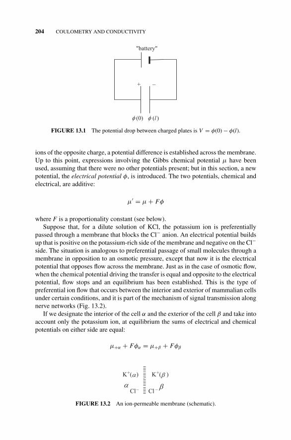
P1: OTA/XYZ P2: ABCc13 JWBS043-Rogers September 13, 2010 11:27 Printer Name: Yet to Come
204 COULOMETRY AND CONDUCTIVITY
+ –
(l )
"battery"
(0)
FIGURE 13.1 The potential drop between charged plates is V = φ(0) − φ(l).
ions of the opposite charge, a potential difference is established across the membrane.Up to this point, expressions involving the Gibbs chemical potential µ have beenused, assuming that there were no other potentials present; but in this section, a newpotential, the electrical potential φ, is introduced. The two potentials, chemical andelectrical, are additive:
µ′ = µ + Fφ
where F is a proportionality constant (see below).Suppose that, for a dilute solution of KCl, the potassium ion is preferentially
passed through a membrane that blocks the Cl− anion. An electrical potential buildsup that is positive on the potassium-rich side of the membrane and negative on the Cl−
side. The situation is analogous to preferential passage of small molecules through amembrane in opposition to an osmotic pressure, except that now it is the electricalpotential that opposes flow across the membrane. Just as in the case of osmotic flow,when the chemical potential driving the transfer is equal and opposite to the electricalpotential, flow stops and an equilibrium has been established. This is the type ofpreferential ion flow that occurs between the interior and exterior of mammalian cellsunder certain conditions, and it is part of the mechanism of signal transmission alongnerve networks (Fig. 13.2).
If we designate the interior of the cell α and the exterior of the cell β and take intoaccount only the potassium ion, at equilibrium the sums of electrical and chemicalpotentials on either side are equal:
µ+α + Fφα = µ+β + Fφβ
K+( K) +( )
Cl –Cl–
FIGURE 13.2 An ion-permeable membrane (schematic).

P1: OTA/XYZ P2: ABCc13 JWBS043-Rogers September 13, 2010 11:27 Printer Name: Yet to Come
RESISTIVITY, CONDUCTIVITY, AND CONDUCTANCE 205
We know that, in general, µ = µ◦ + RT ln a; thus, in this case, we have
µ◦+α + Fφα + RT ln a+α = µ◦
+β + Fφβ + RT ln a+β
but µ◦+α = µ◦
+β because we are talking about the same ion, K+, on either side of themembrane. Differences come, not in µ◦
+, which is fixed, but in the potentials φ andthe activities a, which are variable:
Fφα + RT ln a+α = Fφβ + RT ln a+β
F(φα − φβ
) = RT lna+β
a+α
F is called the Faraday constant. It is a conversion factor from charge in coulombsC or millicoulombs mC to moles. The faraday is the charge on 1 mol of electrons,96,485 C mol−1, which may in general be regarded as 1 mol of charge.
Under the stipulation that the concentrations are rather low, the activity coefficientsγ are about equal to 1.0 and we may replace the activities by molarities (or molalities)m to find the membrane potential
(φα − φβ
) = RT
Fln
m+β
m+α
Nerve cell walls are semipermeable, accounting for an equilibrium membranepotential of about 70 mV. This equilibrium potential can be disturbed by an electricalpulse from a neighbor cell, whereupon the pulse is transmitted to another neighborcell in a sequence that is part of the mechanism for transmission of informationalong a nerve fiber.
13.2 RESISTIVITY, CONDUCTIVITY, AND CONDUCTANCE
If a charge suspended in a fluid medium is subjected to a potential difference �φ,it will move. Moving charge is called current I = d Q/dt , where Q is the charge incoulombs. Typically, a moving charge meets resistance R.1 Resistance is proportionalto the length l of a resistor and is inversely proportional to its cross-sectional area A:
R ∝ l
A= ρ
l
A
The proportionality constant ρ = R A/ l is a characteristic of the resistor material. Itis called the resistivity.
These definitions prompt us to define the inverse of the resistance called theconductance L ≡ 1/R, along with the inverse of the resistivity, the conductivityκ ≡ 1/ρ:
L ≡ 1
R= A
ρ l= κ A
l
1We shall not consider superconductive media here.
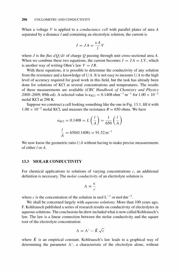
P1: OTA/XYZ P2: ABCc13 JWBS043-Rogers September 13, 2010 11:27 Printer Name: Yet to Come
206 COULOMETRY AND CONDUCTIVITY
When a voltage V is applied to a conductance cell with parallel plates of area Aseparated by a distance l and containing an electrolyte solution, the current is
I = J A = κ A
lV
where J is the flux d Q/dt of charge Q passing through unit cross-sectional area A.When we combine these two equations, the current becomes I = J A = LV , whichis another way of writing Ohm’s law V = I R.
With these equations, it is possible to determine the conductivity of any solutionfrom the resistance and a knowledge of l/A. It is not easy to measure l/A to the highlevel of accuracy required for good work in this field, but the task has already beendone for solutions of KCl at several concentrations and temperatures. The resultsof these measurements are available (CRC Handbook of Chemistry and Physics2008–2009, 89th ed). A selected value is κKCl = 0.1408 ohm−1 m−1 for 1.00 × 10⁻²
molal KCl at 298 K.Suppose we construct a cell looking something like the one in Fig. 13.1, fill it with
1.00 × 10⁻² molal KCl, and measure the resistance R = 650 ohms. We have
κKCl = 0.1408 = L
(l
A
)= 1
650
(l
A
)
l
A= 650(0.1408) = 91.52 m−1
We now know the geometric ratio l/A without having to make precise measurementsof either l or A.
13.3 MOLAR CONDUCTIVITY
For chemical applications to solutions of varying concentrations c, an additionaldefinition is necessary. The molar conductivity of an electrolyte solution is
� ≡ κ
c
where c is the concentration of the solution in mol L−1 or mol dm−3.We shall be concerned largely with aqueous solutions. More than 100 years ago,
F. Kohlrausch published a series of research results on conductivity of electrolytes inaqueous solutions. The conclusions he drew included what is now called Kohlrausch’slaw. The law is a linear connection between the molar conductivity and the squareroot of the electrolyte concentration:
� = �◦ − K√
c
where K is an empirical constant. Kohlrausch’s law leads to a graphical way ofdetermining the parameter �◦, a characteristic of the electrolyte alone, without
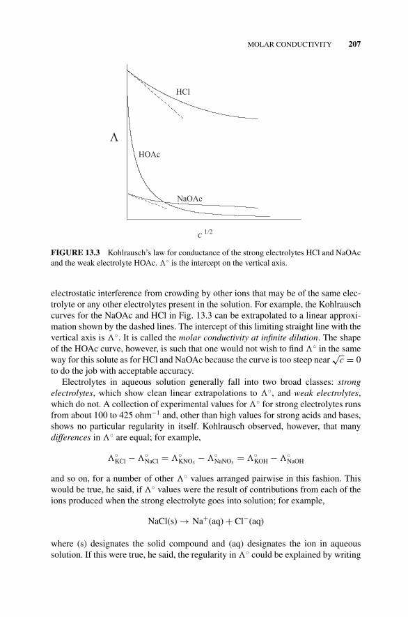
P1: OTA/XYZ P2: ABCc13 JWBS043-Rogers September 13, 2010 11:27 Printer Name: Yet to Come
MOLAR CONDUCTIVITY 207
HCl
HOAc
NaOAc
c 1/2
FIGURE 13.3 Kohlrausch’s law for conductance of the strong electrolytes HCl and NaOAcand the weak electrolyte HOAc. �◦ is the intercept on the vertical axis.
electrostatic interference from crowding by other ions that may be of the same elec-trolyte or any other electrolytes present in the solution. For example, the Kohlrauschcurves for the NaOAc and HCl in Fig. 13.3 can be extrapolated to a linear approxi-mation shown by the dashed lines. The intercept of this limiting straight line with thevertical axis is �◦. It is called the molar conductivity at infinite dilution. The shapeof the HOAc curve, however, is such that one would not wish to find �◦ in the sameway for this solute as for HCl and NaOAc because the curve is too steep near
√c = 0
to do the job with acceptable accuracy.Electrolytes in aqueous solution generally fall into two broad classes: strong
electrolytes, which show clean linear extrapolations to �◦, and weak electrolytes,which do not. A collection of experimental values for �◦ for strong electrolytes runsfrom about 100 to 425 ohm−1 and, other than high values for strong acids and bases,shows no particular regularity in itself. Kohlrausch observed, however, that manydifferences in �◦ are equal; for example,
�◦KCl − �◦
NaCl = �◦KNO3
− �◦NaNO3
= �◦KOH − �◦
NaOH
and so on, for a number of other �◦ values arranged pairwise in this fashion. Thiswould be true, he said, if �◦ values were the result of contributions from each of theions produced when the strong electrolyte goes into solution; for example,
NaCl(s) → Na+(aq) + Cl−(aq)
where (s) designates the solid compound and (aq) designates the ion in aqueoussolution. If this were true, he said, the regularity in �◦ could be explained by writing
P1: OTA/XYZ P2: ABCc13 JWBS043-Rogers September 13, 2010 11:27 Printer Name: Yet to Come
208 COULOMETRY AND CONDUCTIVITY
the contributions to �◦ as
�◦KCl = λ◦
K+ + λ◦Cl−
�◦NaCl = λ◦
Na+ + λ◦Cl−
...
and so on.
In this way, the difference found for
�◦KCl − �◦
NaCl = �◦KNO3
− �◦NaNO3
would be merely the difference
�◦KCl − �◦
NaCl = λ◦Na+ + λ◦
Cl− − λ◦K+ − λ◦
Cl−
= λ◦Na+ − λ◦
K+
and would be the same for all pairs of sodium and potassium electrolytes because theanions, Cl−, NO−
3 , OH−. . . , would always cancel out. The same would be true forpairs of electrolytes containing a common anion, because the cation would alwayscancel out. In these and similar calculations, the integral charge on an ion must alwaysbe taken into account so that the expression for Kohlrausch’s law of independent ionmigration is
�◦ = ν+λ+ + ν−λ−
where ν is the number of charges on each ion, ν = 1 for the examples shown.
13.4 PARTIAL IONIZATION: WEAK ELECTROLYTES
So far we have considered mainly strong electrolytes, those for which ionizationis complete in aqueous solution. This is not always the case. Ionization of weakelectrolytes is partial. The usual example chosen is that of acetic acid for whichionization at ordinary concentrations is very small. Examples of the vast difference inbehavior can be seen by comparing the Kohlrausch conductivity curves in Fig. 13.3for HCl, which is completely ionized, with that of acetic acid (HOAc), which is not.Ionization of HOAc does, however, rise rapidly in dilute solutions, and Kohlrausch’slaw of independent migration holds at infinite dilution. At infinite dilution, the weakelectrolyte HOAc is completely dissociated (all electrolytes are), so we have a verysimple way of determining the approximate degree of ionization α at some finiteconcentration c by comparing � to �◦. We simply take the ratio
α = �
�◦
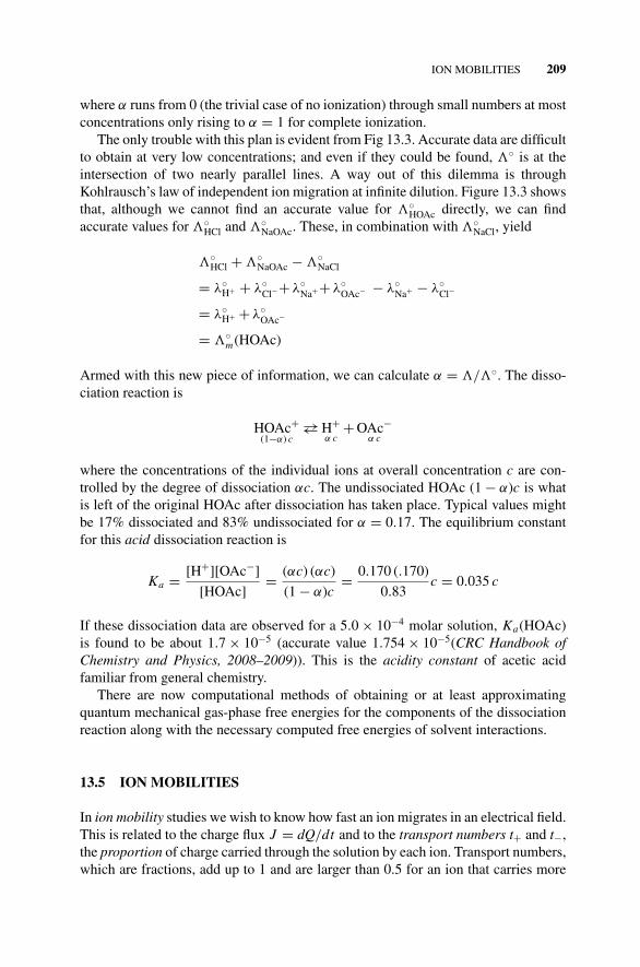
P1: OTA/XYZ P2: ABCc13 JWBS043-Rogers September 13, 2010 11:27 Printer Name: Yet to Come
ION MOBILITIES 209
where α runs from 0 (the trivial case of no ionization) through small numbers at mostconcentrations only rising to α = 1 for complete ionization.
The only trouble with this plan is evident from Fig 13.3. Accurate data are difficultto obtain at very low concentrations; and even if they could be found, �◦ is at theintersection of two nearly parallel lines. A way out of this dilemma is throughKohlrausch’s law of independent ion migration at infinite dilution. Figure 13.3 showsthat, although we cannot find an accurate value for �◦
HOAc directly, we can findaccurate values for �◦
HCl and �◦NaOAc. These, in combination with �◦
NaCl, yield
�◦HCl + �◦
NaOAc − �◦NaCl
= λ◦H+ + λ◦
Cl−+ λ◦Na++ λ◦
OAc− − λ◦Na+ − λ◦
Cl−
= λ◦H+ + λ◦
OAc−
= �◦m(HOAc)
Armed with this new piece of information, we can calculate α = �/�◦. The disso-ciation reaction is
HOAc+(1−α) c
→← H+α c
+ OAc−α c
where the concentrations of the individual ions at overall concentration c are con-trolled by the degree of dissociation αc. The undissociated HOAc (1 − α)c is whatis left of the original HOAc after dissociation has taken place. Typical values mightbe 17% dissociated and 83% undissociated for α = 0.17. The equilibrium constantfor this acid dissociation reaction is
Ka = [H+][OAc−]
[HOAc]= (αc) (αc)
(1 − α)c= 0.170 (.170)
0.83c = 0.035 c
If these dissociation data are observed for a 5.0 × 10⁻⁴ molar solution, Ka(HOAc)is found to be about 1.7 × 10⁻⁵ (accurate value 1.754 × 10⁻⁵(CRC Handbook ofChemistry and Physics, 2008–2009)). This is the acidity constant of acetic acidfamiliar from general chemistry.
There are now computational methods of obtaining or at least approximatingquantum mechanical gas-phase free energies for the components of the dissociationreaction along with the necessary computed free energies of solvent interactions.
13.5 ION MOBILITIES
In ion mobility studies we wish to know how fast an ion migrates in an electrical field.This is related to the charge flux J = dQ/dt and to the transport numbers t+ and t−,the proportion of charge carried through the solution by each ion. Transport numbers,which are fractions, add up to 1 and are larger than 0.5 for an ion that carries more
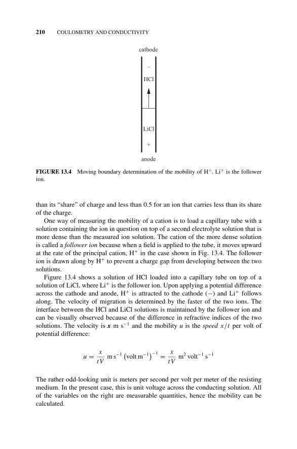
P1: OTA/XYZ P2: ABCc13 JWBS043-Rogers September 13, 2010 11:27 Printer Name: Yet to Come
210 COULOMETRY AND CONDUCTIVITY
+
–
HCl
LiCl
cathode
anode
FIGURE 13.4 Moving boundary determination of the mobility of H+. Li+ is the followerion.
than its “share” of charge and less than 0.5 for an ion that carries less than its shareof the charge.
One way of measuring the mobility of a cation is to load a capillary tube with asolution containing the ion in question on top of a second electrolyte solution that ismore dense than the measured ion solution. The cation of the more dense solutionis called a follower ion because when a field is applied to the tube, it moves upwardat the rate of the principal cation, H+ in the case shown in Fig. 13.4. The followerion is drawn along by H+ to prevent a charge gap from developing between the twosolutions.
Figure 13.4 shows a solution of HCl loaded into a capillary tube on top of asolution of LiCl, where Li+ is the follower ion. Upon applying a potential differenceacross the cathode and anode, H+ is attracted to the cathode (−) and Li+ followsalong. The velocity of migration is determined by the faster of the two ions. Theinterface between the HCl and LiCl solutions is maintained by the follower ion andcan be visually observed because of the difference in refractive indices of the twosolutions. The velocity is x m s−1 and the mobility u is the speed x/t per volt ofpotential difference:
u = x
tVm s−1
(volt m−1
)−1 = x
tVm2 volt−1 s−1
The rather odd-looking unit is meters per second per volt per meter of the resistingmedium. In the present case, this is unit voltage across the conducting solution. Allof the variables on the right are measurable quantities, hence the mobility can becalculated.
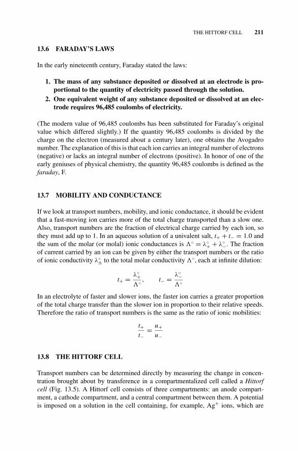
P1: OTA/XYZ P2: ABCc13 JWBS043-Rogers September 13, 2010 11:27 Printer Name: Yet to Come
THE HITTORF CELL 211
13.6 FARADAY’S LAWS
In the early nineteenth century, Faraday stated the laws:
1. The mass of any substance deposited or dissolved at an electrode is pro-portional to the quantity of electricity passed through the solution.
2. One equivalent weight of any substance deposited or dissolved at an elec-trode requires 96,485 coulombs of electricity.
(The modern value of 96,485 coulombs has been substituted for Faraday’s originalvalue which differed slightly.) If the quantity 96,485 coulombs is divided by thecharge on the electron (measured about a century later), one obtains the Avogadronumber. The explanation of this is that each ion carries an integral number of electrons(negative) or lacks an integral number of electrons (positive). In honor of one of theearly geniuses of physical chemistry, the quantity 96,485 coulombs is defined as thefaraday, F.
13.7 MOBILITY AND CONDUCTANCE
If we look at transport numbers, mobility, and ionic conductance, it should be evidentthat a fast-moving ion carries more of the total charge transported than a slow one.Also, transport numbers are the fraction of electrical charge carried by each ion, sothey must add up to 1. In an aqueous solution of a univalent salt, t+ + t− = 1.0 andthe sum of the molar (or molal) ionic conductances is �◦ = λ◦
+ + λ◦−. The fraction
of current carried by an ion can be given by either the transport numbers or the ratioof ionic conductivity λ◦
± to the total molar conductivity �◦, each at infinite dilution:
t+ = λ◦+
�◦ , t− = λ◦−
�◦
In an electrolyte of faster and slower ions, the faster ion carries a greater proportionof the total charge transfer than the slower ion in proportion to their relative speeds.Therefore the ratio of transport numbers is the same as the ratio of ionic mobilities:
t+t−
= u+u−
13.8 THE HITTORF CELL
Transport numbers can be determined directly by measuring the change in concen-tration brought about by transference in a compartmentalized cell called a Hittorfcell (Fig. 13.5). A Hittorf cell consists of three compartments: an anode compart-ment, a cathode compartment, and a central compartment between them. A potentialis imposed on a solution in the cell containing, for example, Ag+ ions, which are
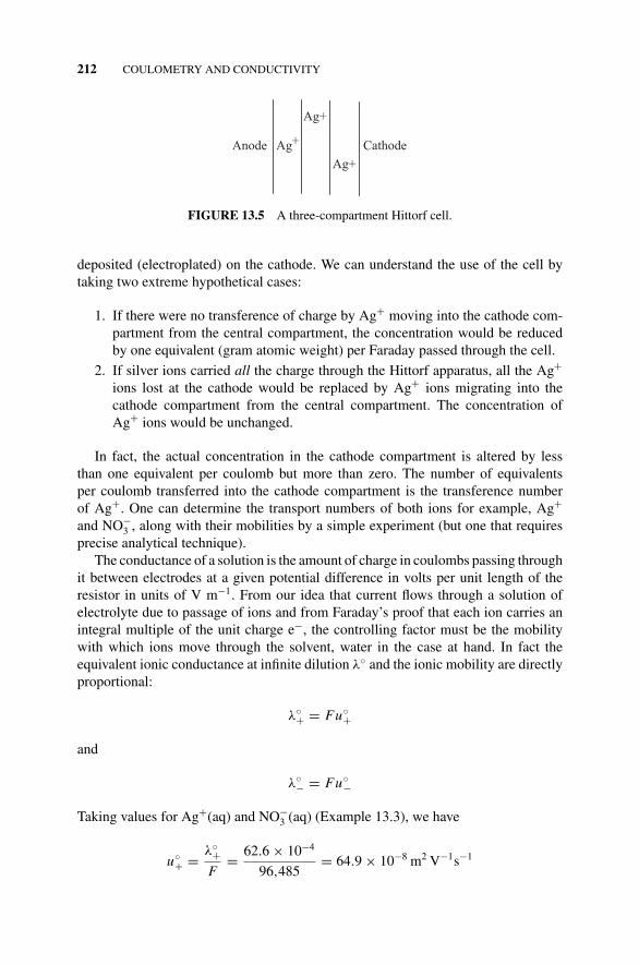
P1: OTA/XYZ P2: ABCc13 JWBS043-Rogers September 13, 2010 11:27 Printer Name: Yet to Come
212 COULOMETRY AND CONDUCTIVITY
Anode Ag+ Cathode
Ag+
Ag+
FIGURE 13.5 A three-compartment Hittorf cell.
deposited (electroplated) on the cathode. We can understand the use of the cell bytaking two extreme hypothetical cases:
1. If there were no transference of charge by Ag+ moving into the cathode com-partment from the central compartment, the concentration would be reducedby one equivalent (gram atomic weight) per Faraday passed through the cell.
2. If silver ions carried all the charge through the Hittorf apparatus, all the Ag+
ions lost at the cathode would be replaced by Ag+ ions migrating into thecathode compartment from the central compartment. The concentration ofAg+ ions would be unchanged.
In fact, the actual concentration in the cathode compartment is altered by lessthan one equivalent per coulomb but more than zero. The number of equivalentsper coulomb transferred into the cathode compartment is the transference numberof Ag+. One can determine the transport numbers of both ions for example, Ag+
and NO−3 , along with their mobilities by a simple experiment (but one that requires
precise analytical technique).The conductance of a solution is the amount of charge in coulombs passing through
it between electrodes at a given potential difference in volts per unit length of theresistor in units of V m−1. From our idea that current flows through a solution ofelectrolyte due to passage of ions and from Faraday’s proof that each ion carries anintegral multiple of the unit charge e−, the controlling factor must be the mobilitywith which ions move through the solvent, water in the case at hand. In fact theequivalent ionic conductance at infinite dilution λ◦ and the ionic mobility are directlyproportional:
λ◦+ = Fu◦
+
and
λ◦− = Fu◦
−
Taking values for Ag+(aq) and NO−3 (aq) (Example 13.3), we have
u◦+ = λ◦
+F
= 62.6 × 10⁻⁴
96,485= 64.9 × 10⁻⁸ m2 V−1s−1
P1: OTA/XYZ P2: ABCc13 JWBS043-Rogers September 13, 2010 11:27 Printer Name: Yet to Come
ION ACTIVITIES 213
and
u◦− = λ◦
−F
= 70.6 × 10⁻⁴
96,485= 73.2 × 10⁻⁸ m2 V−1 s−1
These unusual units deserve a note. The units of speed m s−1 can be split off:
m2 V−1 s−1 = mV−1(m s−1
)
and
(m s−1) mV−1 = m s−1 1(
Vm−1)
In other words, the unit is a typical speed in meters per second per unit voltagedrop measured in volts per meter in the MKS system for the separation between theelectrodes in the cell.
13.9 ION ACTIVITIES
One would like to have activities and activity coefficients for single ion concentrationsto use just as activities, and activity coefficients were used for single moleculeconcentrations in Chapters 7 and 12. Unfortunately, this is not possible becausesingle ions cannot be observed in the absence of a partner ion necessary to preserveelectroneutrality. Faced with this dilemma, we make an approximation that ionicactivities are equal: a+ = a−. This is obviously not true, but it is the best we can do.The best we can find is an average activity, the geometric mean, a± ≡ √
a+a−. Otherdefinitions follow as they did for simple molecules: a± = γ±m, γ± ≡ √
γ+γ−, and
γ± ≡√
a+m
a−m
= a±m
Debye and Huckel have given a rather involved treatment of the electrostatic forcesacting on an ion surrounded by other ions. They arrived at an expression for γ± inthe form of the Debye–Huckel limiting law:
ln γ± = −1.172 |Z+ Z−| √µ
where – 1.172 is a combination of constants, |Z+ Z−| is the product of atomic charges(|Z+ Z−| = 1.0 in the cases we consider here), and
õ is a concentration term which
is the summation of all the surrounding electrolytes, not just the electrolyte for whichwe seek γ±. The symbol µ is almost universally used to denote both Debye–Huckelionic strength and Gibbs chemical potential. To diminish this source of confusion,
P1: OTA/XYZ P2: ABCc13 JWBS043-Rogers September 13, 2010 11:27 Printer Name: Yet to Come
214 COULOMETRY AND CONDUCTIVITY
we are using the notation µ for the ionic strength:
µ = 12
∑i
mi Z2i
The Debye–Huckel law is applicable only in very dilute solutions; it is a typicallimiting law.
We know how to determine the ionization constant Ka for weak acids, say aceticacid, but we find upon close examination that the results are not quite constant withdifferent concentrations of HOAc, and we presume that this lack is due to interferenceamong ions. This nonideality can be expressed in terms of ionic activities:
Ka = aH+aOAc−
aHOAc= γ±mH+γ±mOAc−
γ mHOAc
In this model, nonideality is caused by charge interaction but HOAc is uncharged, sowe can consider it an ideal solute and take γHOAc = 1.0. The ions, however, are notideal. This means that γ± = 1.0, so
Ka = aH+aOAc−
aHOAc= γ±mH+γ±mOAc−
γHOAcmHOAc= γ 2
±m2
H+
mHOAc= γ 2
±K
where mOAc− = mH+ because equal numbers of product ions H+ and OAc− areproduced in the dissociation reaction
HOAc →← H+ + OAc−
Taking logarithms of both sides, we obtain
ln Ka = 2 ln γ± + ln K
where K is a measured (nonideal) value for the acid dissociation constant and Ka isthe ideal value. At infinite dilution, γ± = 1.0 and ln γ± = 0.0, so
ln K︸︷︷︸m→0
= ln Ka
For a dilute acid in pure water, each ion concentration is αm, where α is thedegree of dissociation and m is the molar concentration of acid (Section 13.4). Theionic strength is determined by the concentration of ions in the solution, but this isby no means the bulk concentration of acid. Many acids—for example, acetic acidHOAc—ionize to a very limited extent, but even ionization of pure water contributesto the ionic strength. According to the Debye–Huckel limiting law, we have
ln γ± = −1.172√
µ = −1.172√
αm
P1: OTA/XYZ P2: ABCc13 JWBS043-Rogers September 13, 2010 11:27 Printer Name: Yet to Come
PROBLEMS AND EXAMPLES 215
for the acid. The acidity (ionization) constant is
ln Ka = 2 ln γ± + ln K
ln Ka = 2(−1.172
√αm
) + ln K = −2.34√
αm + ln K
or
ln K = −2.34√
αm + ln Ka
A plot of ln K vs.√
αm gives an intercept of ln Ka and has a limiting slope of 2.34as α → 1. As m becomes very small, the middle term of ln K = 2.34
√αm + ln Ka
drops out and the measured value of K approaches Ka .
PROBLEMS AND EXAMPLES
Example 13.1
Suppose you have access to a well-equipped electrochemistry laboratory but you donot know the value of the faraday. How would you determine the value of the faradayto four significant figures?
Solution 13.1 To work the problem de novo would be a pretty hard job. Remember,Faraday was a genius. When you electrolyze different solutions, however, you willsoon find that many metals including silver can be plated out on an electrode bypassage of current through a solution of, for example, silver nitrate. A coulomb isan ampere second. The idea is this: Measure the current flow I times the time t inseconds to force the quantity Q of electricity in coulombs through an electrolysis cellto plate the silver. Then measure the number of moles of silver that have been platedout. The fraction I × t/moles Ag gives the faraday in coulombs mol−1. Your first tryat this method will probably be unsuccessful because the faraday is a big number.It takes more electricity than you might guess to deposit an amount of silver that ismeasurable to four figures of accuracy.
Many electrochemical laboratories are equipped with a variety of potentiostats thatmaintain a constant voltage across an experimental cell and amperostats that maintaina constant current. For our purposes, an amperostat would be most convenient becauseintegration to find the area under an I vs. t curve would merely be multiplying constantI into the time. Both of these measurements should be possible with high accuracy.Silver has been known for many years to be plated out in 100% current efficiency,so if we multiply our I measurement into the time of electrolysis, both measureddigitally, we get the number of coulombs passed through the cell. We can then weighthe silver electrode and find out how much it has increased in weight due to the silverdeposited.
To get a rough idea of the parameters involved, suppose we have a microbalancesensitive and accurate enough to weigh to ±0.01 mg. A silver weight of 0.2 g would
P1: OTA/XYZ P2: ABCc13 JWBS043-Rogers September 13, 2010 11:27 Printer Name: Yet to Come
216 COULOMETRY AND CONDUCTIVITY
be within our measurement range. If the amount of current we can maintain is about50 milliamperes (mA), we know everything in the equation except the time. Trialsshow that it takes about an hour (1 h = 3600 s) to deposit 0.2 g of Ag.
F = I × t
moles Ag= 0.050 × 3600
0.2
107.9
= 180
0.00185= 97,110
Now in our precise one-hour experiment, the real amperostat reading is 49.883 mAover the time period of 1.000 h = 3600.0 s, and the weight of silver gained by the(carefully dried) silver cathode is 0.20149 g
F = coulombs
mol= I × t
mol= 0.049883 (3600.00)
0.20101
107.868
= 179.5788
0.00186534= 96,367
which is a little more than 0.1% in error.
Example 13.2
Suppose you are in the unlikely circumstance of needing to know the faraday to ninesignificant figures. Propose a way of calculating F from fundamental constants.
Solution 13.2 Unknown in Faraday’s time, of course, unit charge is 1.602176487 ×10⁻¹⁹ C and Avogadro’s number is NA = 6.02214179 × 10²³. Since the faraday isthe charge per mole of (singly charged) particles, we have
F = (6.02214179 × 10²³
)1.602176487 × 10−19 = 96485.3398 C mol−1
These data are from the handbook, but you will get some argument on the last twodigits.
Example 13.3
(a) A Hittorf cell having 0.1000 mol of AgNO3(aq) in each of its three compart-ments had 0.0100 faradays of charge passed through it. A reduction reactiondepositing solid silver, Ag(s), took place at the cathode:
Ag+(aq) + e− → Ag(s)
Analysis of the contents of the cathode compartment after the experimentshowed that 0.00947 mol of Ag+(aq) remained. What are the transport num-bers of Ag+(aq) and NO−
3 (aq)?
P1: OTA/XYZ P2: ABCc13 JWBS043-Rogers September 13, 2010 11:27 Printer Name: Yet to Come
PROBLEMS AND EXAMPLES 217
(b) Given the additional information that �◦AgNO3
= 133.3 × 10⁻⁴ ohm−1
m2 mol−1, what are the molar ionic conductivities and mobilities of Ag+(aq)and NO−
3 (aq)?
Solution 13.3
(a) If the Ag+(aq) ions did not move, the amount of silver ion found in thecathode compartment after electrolysis would have been 0.0900 mols becauseof the removal of 0.0100 mol of Ag+(aq) by electrodeposition. The fact thatthere are 0.0947 mol in the cathode compartment after deposition means that0.0047 mol of Ag+(aq) have been replaced by Ag+(aq) migration from thecenter compartment. The transport number is the ratio of the charge transferredby Ag+(aq) transport relative to the total charge transferred by both ions:
t+ = 0.0047
0.0100= 0.47
The rest of transport must have been due to NO−3 (aq) ions migrating in the
opposite direction, so t− = 1.00 − 0.47 = 0.53.
(b) Transport numbers are related to ionic conductances according to the equations
t+ = λ◦+
�◦ t− = λ◦−
�◦
which is reasonable because an ion that transports more than its share ofcharge will have a large ionic conductivity relative to the total �◦. Given that�◦
AgNO3= 133.3 × 10⁻⁴ ohm−1 m2 mol−1, we obtain
λ◦+ = t+�◦ = 0.47
(133.3 × 10⁻⁴
) = 62.6 × 10⁻⁴ ohm−1 m2 mol−1
and
λ◦− = t− �◦ = 0.53
(133.3 × 10⁻⁴) = 70.6 × 10⁻⁴ ohm−1 m2 mol−1
Problem 13.1
A solution containing 1.155 × 10⁻² mol of HCl was neutralized by adding NaOHsolution. The process brought about a 0.553 K temperature rise. An electrical heaterof 58.7-ohm resistance brought about a 0.487 K temperature rise in 15.0 min. Apotential of 6.03 volts was maintained across the resistor by a potentiostat. What isthe molar enthalpy of HCl? Remember that a joule is a volt coulomb.

P1: OTA/XYZ P2: ABCc13 JWBS043-Rogers September 13, 2010 11:27 Printer Name: Yet to Come
218 COULOMETRY AND CONDUCTIVITY
Problem 13.2
What is the charge on the silver ions in 1.000 dm3 of dissolved Ag+ in aqueoussolution equilibrium with Cl− and solid AgCl(s) at 298 K? The solubility productconstant of AgCl is Ksp = 1.77 × 10⁻⁵. There is no outside source of Cl− ion.
Problem 13.3
l-Dopa (l-(dihydroxyphenyl)alanine) is used to treat the symptoms of Parkinson’sdisease. It is quantitatively and exhaustively reduced in an electrolysis cell, requir-ing two electrons per molecule. Its molar mass is M = 0.1972 kg mol−1. Supposea sample requires 57.5 µC (microcoulombs) for complete reduction. How muchl-dopa was in the sample?
Problem 13.4
The resistivity of copper at 298 K is ρ = 1.71 × 10⁻⁸ ohm m. A potential of 1.00 mVwas placed across a copper wire 1.00 mm in diameter and 1.00 m long. What was thecurrent?
Problem 13.5
(a) The resistivity of copper at 298 K is ρ = 1.71 × 10⁻⁸ ohm m. Find theconductance and the conductivity of a copper wire 1.00 mm in diameterand 1.00 m long.
(b) Find the conductance and the conductivity of a copper wire 2.00 mm indiameter and .500 m long.
Problem 13.6
A conductivity cell is constructed using two platinum electrodes, precisely machinedto be a square 2 cm on an edge and 1 cm apart. A 0.1000 mol dm−3 HCl solution waspoured into the cell, and the resistance was measured and found to be 6.3882 ohms.What is the molar conductivity of HCl at this concentration? In solving this problem,be careful to express the units clearly at each step.
Problem 13.7
We can write the ionization of water in a somewhat simplified form as
H2O → H+ + OH−
The conductivity of deionized water is κ = 5.50 × 10⁻⁶ ohm−1 m2 mol−1.
(a) Find the concentration c of pure water in mol dm−3.
(b) Find the degree of ionization α.
P1: OTA/XYZ P2: ABCc13 JWBS043-Rogers September 13, 2010 11:27 Printer Name: Yet to Come
PROBLEMS AND EXAMPLES 219
(c) Find the equilibrium constant Kw for the dissociation of pure water.
(d) Find the concentration of hydrogen ions H+ in pure water.
(e) Why is it meaningful to calculate the equilibrium constant for H+ even thoughwe know that H3O+, H5O+, . . . also exist in pure water?
Problem 13.8
The molar conductivities of NaCl are given in the handbook as
mol dm−3 Conductivity mol dm−3 Conductivity
5.0000e-4 124.4400 1.0000e-3 123.68005.0000e-3 120.5900 0.0100 118.45000.0200 115.7000 0.0500 111.01000.1000 106.6900
Plot these data in the form of a Kohlrausch plot. Determine the value of �◦NaCl and
the slope of the linear extrapolation to �◦NaCl.
Problem 13.9
The molar conductivities �◦ of NH4 Cl, NaOH, and NaCl are 149.6, 247.7, and126.4 in units of 104 S m2 mol−1. Find �◦
NH4OH.
Problem 13.10
Show that the units of conductivity κ are ohm−1 m−1.
Problem 13.11
One meaning of the term Gibbs free energy is that �G is the maximum work thatcan be obtained from a chemical reaction. Conversely, the negative of �G is theminimum work that must be put into a chemical system to reverse its direction. Giventhat �G = −237 kJ mol−1 for the spontaneous reaction (note the sign of �G)
H2(g) + 12 O2(g) → H2O(l)
and the fact that work w = charge(V) where the charge is in coulombs and V is thevoltage, find the minimum potential in volts necessary for the electrolysis of water toform H2(g) + 1
2 O2(g).
P1: OTA/XYZ P2: ABCc14 JWBS043-Rogers September 13, 2010 11:27 Printer Name: Yet to Come
14ELECTROCHEMICAL CELLS
Advances in electrochemistry came at least a generation earlier than correspondingadvances in rigorous thermochemical theory. Even prior to Faraday’s numerous dis-coveries, Alessandro Volta’s experiments on static electricity and electrical currenttook place largely in the eighteenth century and culminated in the first true battery ofseries voltaic cells. The battery was called a voltaic pile because cells were piled ontop of one another. Volta’s work excited great popular interest, especially when heshowed that Luigi Galvani’s use of a voltaic pile to activate nervous response in thedissected leg of a dead frog depended on the electrical potential of the pile and wasnot a property of the frog’s leg. Activation of a dead animal raised the question ofwhether science might someday actually produce life.1 News of Volta’s experimentsbecame something of a fad of the day. Mary Shelley’s popular creation Frankensteinwas presumably electrochemically activated.
14.1 THE DANIELL CELL
If you put a zinc rod into a solution of zinc sulfate ZnSO4, there will be a differencein chemical potential between the Zn(s) in the metal rod and the Zn2+(aq) ion in theaqueous solution. A reaction takes place, causing a minute amount of Zn to dissolveand go from the rod into the solution, leaving two electrons behind or, depending on
1See Gibson, D. G. et al. 2010. Science, 329, 52–56 for a claim that science has produced life.
Concise Physical Chemistry, by Donald W. RogersCopyright C© 2011 John Wiley & Sons, Inc.
220
P1: OTA/XYZ P2: ABCc14 JWBS043-Rogers September 13, 2010 11:27 Printer Name: Yet to Come
HALF-CELLS 221
concentration, causing Zn2+(aq) to go from the solution onto the rod, taking up twoelectrons from the metal:
Zn(s) → Zn2+(aq) + 2e−
or
Zn2+(aq) + 2e− → Zn(s)
Either way, an electrical potential difference is produced between the electrode and thesolution such that the sum of the chemical potential and the electrical potential, calledthe electrochemical potential, on one side balances the electrochemical potential onthe other side, and equilibrium is reached.
If the same thing is done using a copper rod in contact with a CuSO4 solution,an electrochemical balance is quickly reached in the same way, but the electricalpotential on the Cu electrode is not the same as it was on the Zn electrode becausethe chemical potential of solid Cu is not the same as it is for solid Zn(s). Zn(s) is saidto be more active than Cu(s) because it has a greater tendency to dissolve in a dilutesolution of its ions than Cu(s). If a Zn; Zn2+electrode at potential φ is connected to aCu; Cu2+ electrode across a digital voltmeter and the circuit is completed by meansof a neutral salt bridge, the difference in potential, called the voltage of the cell, canbe measured. It turns out to be about 1.1 volts, depending on the concentrations of theZnSO4 and CuSO4 in the electrode compartments. The entire arrangement is calleda Daniell cell.2
If a resistance or small motor replaces the digital voltmeter, heat or work can beobtained. This is the principle of all electrochemical cells. Historically, two or morecells connected were called a battery of cells by analogy to gun batteries. What wecall the 1.5-volt AA “battery” is really a single cell.
14.2 HALF-CELLS
There are a great variety of cells available for research and practical use. The Cu; Cu2+
and Zn; Zn2+electrodes can be replaced by other metals, leading to many metal–metalion combinations. These M; Mz+ systems, where z is the number of electrons in-volved in the electrode reaction, are called half-cells because any two of them canbe combined to form a cell. The semicolon is used to denote the possibility ofelectron exchange and is often, but not necessarily, a physical interface such as thesolid;solution interface in Zn; Zn2+. The electrochemical standard is the hydrogenhalf-cell (Fig. 14.1). Hydrogen is allowed to pass through the cell under 1 atm
2Invented as early as 1837. The original Daniell cell was a copper cup containing the CuSO4 in whicha porous cup containing the Zn;Zn2+ solution was suspended. The porous cup soaked with salt solutiontook the place of the salt bridge. The Daniell cell had many practical uses and played an important part inearly electrochemistry.
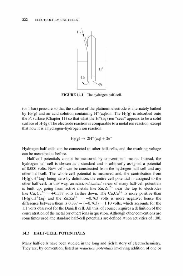
P1: OTA/XYZ P2: ABCc14 JWBS043-Rogers September 13, 2010 11:27 Printer Name: Yet to Come
222 ELECTROCHEMICAL CELLS
H2
H2
Pt
H+
FIGURE 14.1 The hydrogen half-cell.
(or 1 bar) pressure so that the surface of the platinum electrode is alternately bathedby H2(g) and an acid solution containing H+(aq)ion. The H2(g) is adsorbed ontothe Pt surface (Chapter 11) so that what the H+(aq) ion “sees” appears to be a solidsurface of H2(g). The electrode reaction is comparable to a metal ion reaction, exceptthat now it is a hydrogen–hydrogen ion reaction:
H2(g) → 2H+(aq) + 2e−
Hydrogen half-cells can be connected to other half-cells, and the resulting voltagecan be measured as before.
Half-cell potentials cannot be measured by conventional means. Instead, thehydrogen half-cell is chosen as a standard and is arbitrarily assigned a potentialof 0.000 volts. Now cells can be constructed from the hydrogen half-cell and anyother half-cell. The whole-cell potential is measured and, the contribution fromH2(g); H+(aq) being zero by definition, the entire cell potential is assigned to theother half-cell. In this way, an electrochemical series of many half-cell potentialsis built up, going from active metals like Zn; Zn2+ near the top to electrodeslike Cu; Cu2+ = +0.337 volts farther down. The Cu;Cu2+ is more positive thanH2(g); H+(aq) and the Zn;Zn2+ = −0.763 volts is more negative; hence thedifference between them is 0.337 − (−0.763) = 1.10 volts, which accounts for the1.1 volts observed for the Daniell cell. All this, of course, requires a definition of theconcentration of the metal (or other) ions in question. Although other conventions aresometimes used, the standard half-cell potentials are defined at ion activities of 1.00.
14.3 HALF-CELL POTENTIALS
Many half-cells have been studied in the long and rich history of electrochemistry.They are, by convention, listed as reduction potentials involving addition of one or
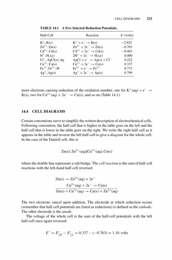
P1: OTA/XYZ P2: ABCc14 JWBS043-Rogers September 13, 2010 11:27 Printer Name: Yet to Come
CELL DIAGRAMS 223
TABLE 14.1 A Few Selected Reduction Potentials.
Half-Cell Reaction E◦(volts)
K+; K(s) K+ + e− → K(s) −2.925Zn2+; Zn(s) Zn2+ + 2e− → Zn(s) −0.763Cd2+; Cd(s) Cd2+ + 2e− → Cd(s) −0.403H+; H2(g) 2H+ + 2e− → H2(g) 0.000Cl−; AgCl(s); Ag AgCl + e− → Ag(s) + Cl− 0.222Cu2+; Cu(s) Cu2+ + 2e− → Cu(s) 0.337Fe3+; Fe2+; Pt Fe3+ + e− → Fe2+ 0.771Ag+; Ag(s) Ag+ + 2e− → Ag(s) 0.799
more electrons causing reduction of the oxidation number, one for K+(aq) + e− →K(s), two for Cu2+(aq) + 2e− → Cu(s), and so on (Table 14.1).
14.4 CELL DIAGRAMS
Certain conventions serve to simplify the written description of electrochemical cells.Following convention, the half-cell that is higher in the table goes on the left and thehalf-cell that is lower in the table goes on the right. We write the right half-cell as itappears in the table and reverse the left half-cell to give a diagram for the whole cell.In the case of the Daniell cell, this is
Zn(s); Zn2+(aq)||Cu2+(aq); Cu(s)
where the double line represents a salt bridge. The cell reaction is the sum of half-cellreactions with the left-hand half-cell reversed:
Zn(s) → Zn2+(aq) + 2e−
Cu2+(aq) + 2e− → Cu(s)
Zn(s) + Cu2+(aq) → Cu(s) + Zn2+(aq)
The two electrons cancel upon addition. The electrode at which reduction occurs(remember that half-cell potentials are listed as reductions) is defined as the cathode.The other electrode is the anode.
The voltage of the whole cell is the sum of the half-cell potentials with the lefthalf-cell once again reversed:
E◦ = E◦12 R
− E◦12 L
= 0.337 − (−0.763) = 1.10 volts
P1: OTA/XYZ P2: ABCc14 JWBS043-Rogers September 13, 2010 11:27 Printer Name: Yet to Come
224 ELECTROCHEMICAL CELLS
This is consistent with our treatment of thermodynamic potentials, for example, wehave
�G◦ = �G◦(B) − �G◦(A)
for the reaction
A → B
The cell reaction, which involves reduction at one electrode and oxidation at the other,is called a reduction–oxidation reaction, or simply a redox reaction. Redox reactionsare spontaneous if written according to the conventions agreed upon.
14.5 ELECTRICAL WORK
A joule is a volt coulomb, so an electrochemical cell operating at 1.0 volt does 1.0 Jof work for every coulomb of electricity it produces. Don’t forget that the coulombC is an amount of charge placed in a capacitor by a specific current in a specifictime C = It. Therefore the number of coulombs is proportional to the number ofelectrons driven through a resistance or motor by the cell reaction. If one electronis exchanged in the cell reaction and one mole of reactant is used up, one mole ofelectrons is exchanged, and one faraday of charge is produced. The work producedis 96,485 joules. In general, n electrons are exchanged and the cell potential isE volts, so
w = nFE = −�G
because the amount of work done per mole of reactant consumed is the molardecrease in the Gibbs free energy. This leads to the important connection betweenthermodynamics and electrochemistry:
�G = −nFE
14.6 THE NERNST EQUATION
For ideal solutions we have
�G = �G◦ + RT ln Q
where Q is the equilibrium quotient, not to be confused with the charge Q. Therefore
nFE = nFE◦ − RT ln Q
P1: OTA/XYZ P2: ABCc14 JWBS043-Rogers September 13, 2010 11:27 Printer Name: Yet to Come
CONCENTRATION CELLS 225
or
E = E◦ − RT
nFln Q
which is the Nernst equation. At 298 K, RT and F can be combined to find
E = E◦ − 0.0257
nln Q
The meanings of �G and �G◦ enable us to better understand E and E◦. As�G is the free energy change for any arbitrary equilibrium quotient Q, E representsthe potential obtained from a cell under these arbitrary conditions. If the reactantsand products are all in their standard states, the difference in free energy betweenreactants and products is �G◦. Hence E◦ represents the potential of a cell in whichthe reactants and products in the redox reaction are in their standard states and at unitactivity. This is just the cell potential from a table of standard half-cell potentials.
Knowing the concentrations of the constituents of any cell not at unit activity, onecan calculate E◦ from the table and correct it to find the actual cell potential usingthe Nernst equation. For example, if the activities in the electrode reaction are
Cu(s) + 2Ag+(aq, 0.01 m) → Cu2+(aq, 0.1 m) + Ag(s)
the equilibrium quotient is Q = Cu2+(aq, 0.1 m)/Ag+(aq, 0.01 m)2 = 0.1/0.012 =1000. The standard cell potential is E◦ = 0.799 − (0.337) = 0.462. Applying theNernst equation with n = 2, we obtain
E = E◦ − 0.0257
nln Q = 0.462 − 0.0128(6.908) = 0.373 volts
Much of the older literature uses the logarithm to the base 10 in the Nernst equation.Conversion from ln to log10 requires multiplication of the ln Q term by 2.303 to yield
E = E◦ − 0.0257
nln Q = E◦ − 2.303 (0.0257)
nlog Q
= 0.462 − 0.0592
23 = 0.343 volts
All of this assumes ideal behavior of course, as well as that a = m throughout. Weshould be skeptical. More about this later.
14.7 CONCENTRATION CELLS
The Nernst equation suggests that we can have an electrochemical cell with half-cells that are identical in every way except for the concentrations of the ions in
P1: OTA/XYZ P2: ABCc14 JWBS043-Rogers September 13, 2010 11:27 Printer Name: Yet to Come
226 ELECTROCHEMICAL CELLS
the electrode compartments. There will be a measurable potential that depends onlyon the difference in concentrations of the aqueous solutions. Such cells are calledconcentration cells.
An example would be any metal;metal ion pair with ion concentrations, sayAg;Ag+(aq) of 0.10 molar in one half-cell and 0.010 m in the other:
Ag(s);Ag+(0.010 m)| |Ag+(0.10 m); Ag(s)
The cell reaction is the half-cell potential of the cathode minus that of the anode (soas to give a positive whole-cell potential):
Ag+(0.10 m) → Ag+(0.010 m)
that is, the direction of spontaneous change for any solution is to become more dilute.(Solutions don’t spontaneously “concentrate themselves.”) Q is 0.010/0.10 = 0.10and the Nernst equation is
E = 0 − 0.0257 ln 0.10 = 0.0592 V = 59.2 mV
If the ion concentration in one of the half-cells is known and the other is unknown,the concentration of the unknown half-cell can be determined from the whole-cellpotential. This is the principle behind the most widely used application of electro-chemistry, the pH meter, in which a potential is measured that is linearly relatedthrough the Nernst equation to the logarithm of the hydrogen ion concentration in ahalf-cell. The negative logarithm (log base 10) of the hydrogen ion concentration is,as we learn in elementary chemistry, the pH. pH meters consist of an H+-sensitive(glass) electrode and a constant voltage (calomel) electrode with suitable electronicsto measure and display or record their algebraic sum. pH meters are calibrated todisplay the hydrogen ion concentration directly in pH units, most frequently as adigital readout.
14.8 FINDING E◦
A silver electrode immersed in a solution of HCl soon becomes covered by a coatingof AgCl(s). This half-cell, connected to a standard hydrogen electrode gives the cell
Pt(s); H2(g); HCl(aq); AgCl(s); Ag(s)
The cell has no need for a salt bridge. One electrode is sensitive to H+ and the otheris sensitive to Cl− which is precisely equal in concentration. The cell reaction is
AgCl(s) + 12 H2(g) →← H+(aq) + Cl−(aq) + Ag(s)
P1: OTA/XYZ P2: ABCc14 JWBS043-Rogers September 13, 2010 11:27 Printer Name: Yet to Come
FINDING E◦ 227
The Nernst equation for this cell is
E = E◦ − RT
Fln
aAgaH+aCl−
aAgClaH2
12
We can set three of these five activities equal to 1.0 because two of them refer to solidsAgCl(s)and Ag(s) and the other has an activity aH2 = 1.0 at a hydrogen pressureof 1.0 atm (or 1.0 bar). The remaining activities are aH+aCl− = γ±mH+γ±mCl− =γ±2mHCl
2, provided that HCl is completely ionized (which it is) and there are noother sources of H+ or Cl−. Now the Nernst equation reads
E = E◦ − RT
Fln aH+aCl− = E◦ − RT
Fln γ±2mHCl
2
= E◦ − 2RT
Fln γ± − 2RT
Fln mHCl
or
E + 2RT
Fln mHCl = E◦ − 2RT
Fln γ±
The right-hand side of this equation approaches E◦ as m approaches zero becauseγ± → 1.0. Plotting E + (2RT/F) ln mHCl as a function of m and extrapolating tom = 0 is appealing, but it is not quite the way the problem is solved. Debye–Huckeltheory (Section 13.9) says that ln γ± = −1.171
√µ where, in this case, µ = m near
infinite dilution. Let us call the term on the left E ′ for convenience in plotting, so that
E ′ =(
E + 2RT
Fln m HCl
)
whereupon
E ′ = E◦ − 2RT (1.171)
Fm1/2
Now we need only plot E ′ as a function of m1/2 to obtain an intercept of E◦ (Fig. 14.2).The plot will yield a straight line with a slope of −2RT (1.171)/F but only inthe limit of infinite dilution. The extrapolation has been carried out with consid-erable precision. It yields 0.22239 volts for the silver chloride–hydrogen cell and,since the standard hydrogen electrode has a half-cell potential of zero by definition,this is equal to the half-cell potential of the silver–silver chloride half-cell listed inTable 14.1.
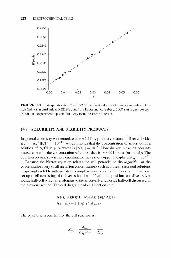
P1: OTA/XYZ P2: ABCc14 JWBS043-Rogers September 13, 2010 11:27 Printer Name: Yet to Come
228 ELECTROCHEMICAL CELLS
m1/2
0.060.050.040.030.020.010.00
E' (
volts
)
0.2220
0.2225
0.2230
0.2235
0.2240
0.2245
0.2250
0.2255
FIGURE 14.2 Extrapolation to E◦ = 0.2223 for the standard hydrogen–silver–silver chlo-ride Cell. (Standard value: 0.22239; data from Klotz and Rosenberg, 2008.) At higher concen-trations the experimental points fall away from the linear function.
14.9 SOLUBILITY AND STABILITY PRODUCTS
In general chemistry we memorized the solubility product constant of silver chloride,Ksp = [Ag+][Cl−] = 10−10, which implies that the concentration of silver ion in asolution of AgCl in pure water is [Ag+] = 10−5. How do you make an accuratemeasurement of the concentration of an ion that is 0.00001 molar (or molal)? Thequestion becomes even more daunting for the case of copper phosphate, Ksp = 10−37.
Because the Nernst equation relates the cell potential to the logarithm of theconcentration, very small metal ion concentrations such as those in saturated solutionsof sparingly soluble salts and stable complexes can be measured. For example, we canset up a cell consisting of a silver–silver ion half-cell in opposition to a silver–silveriodide half-cell which is analogous to the silver–silver chloride half-cell discussed inthe previous section. The cell diagram and cell reactions are
Ag(s); AgI(s); I−(aq)||Ag+(aq); Ag(s)
Ag+(aq) + I−(aq) →← AgI(s)
The equilibrium constant for the cell reaction is
Keq = aAgI
aAg+aI−= 1
Ksp

P1: OTA/XYZ P2: ABCc14 JWBS043-Rogers September 13, 2010 11:27 Printer Name: Yet to Come
THE CALOMEL ELECTRODE 229
where aAgI of the solid precipitate has been set equal to 1.0 and Ksp is the solubilityproduct of the AgI precipitate. The potential of this cell is 0.950 volts and, solvingthe Nernst equation, we find log Ksp = −0.950/0.0592 = −16.0, so Ksp
∼= 10−16.Notice that we use 59.2 mV in the Nernst equation to calculate log10 Ksp (Section14.7). Stability constants of complexes, in which metal ion concentrations are reducedto very low levels by ligands like EDTA, can be measured by a method analogous tothe one shown for AgI.
14.10 MEAN IONIC ACTIVITY COEFFICIENTS
Back calculating from the procedure of Section 14.8 produces γ± at molalities otherthan zero. From
E = E◦ − 2RT
Flog γ± − 2RT
Flog mHCl
E = E◦ − 0.1184 log mHCl − 0.1184 log γ±
and
0.1184 log γ± = −E + E◦ − 0.1184 log mHCl
log γ± = −E + E◦ − 0.1184 log mHCl
0.1184
At finite molality, E can be measured and everything on the right of the equal sign isknown because E◦ is known.
14.11 THE CALOMEL ELECTRODE
The standard hydrogen half-cell has the advantage that its potential is 0.000 bydefinition, but it is bulky and presents some safety hazards in the use of hydrogen.Consequently, several half-cells that do not have these disadvantages are used asreference electrodes. The most common one is the calomel electrode (strictly, half-cell), which is easily set up, is light, and gives a constant voltage at a fixed temperature.Calomel half-cells have liquid mercury in contact with a paste of Hg2Cl2(s) and solidKCl in equilibrium with Cl−(aq). Connection to external circuitry is by a Pt wirein contact with the mercury. Connection with any of a variety of other half-cellsis made through a saturated KCl solution called a salt bridge. The saturated KClsolution does not change much upon drawing a small current, so the output voltageis a constant 0.2444 volts at 298 K. The electrode is designated a saturated calomelelectrode (SCE) from the common name calomel for mercurous chloride (which wasonce used as a medicine for children!!). The cell diagram
Pt; H2(1.0 atm); H+(aq)||Hg2Cl2(s), KCl(aq sat′d); Hg; Pt
P1: OTA/XYZ P2: ABCc14 JWBS043-Rogers September 13, 2010 11:27 Printer Name: Yet to Come
230 ELECTROCHEMICAL CELLS
has a Nernst equation of
Ecell = Ecalomel − 0.0257 ln H+(aq)
because all of the activities other than H+(aq) are 1.0 or are included in Ecalomel. Thisleads to
− ln H+(aq) = Ecell − Ecalomel
0.0257
or, as is more commonly written,
pH ≡ − log H+(aq) = Ecell − Ecalomel
0.0592
These results will not be accurate to an indefinite number of significant figuresbecause the activity coefficient is not exactly 1.0 in real solutions. Cell potentials canbe measured to four or more significant figures, but pH values should be regarded witha prudent degree of skepticism. Conversely, departure of pH values from expectationcan be used to estimate activity coefficients.
14.12 THE GLASS ELECTRODE
We still have the problem of a bulky, somewhat dangerous hydrogen half-cell to de-termine pH in the field. For practical work, the glass electrode is used instead. Withincertain limits, the potential between opposite sides of a very thin glass membranevaries in a linear way with hydrogen ion concentration. This is used in to determinepH, but the nature of the hydrogen ion sensitivity is not rigorously understood beyondknowing that there is an interchange between the aqueous hydrogen ions and the Na+
ions in the glass on one side of the membrane that is different from the interchangeon the other. Consequently, pH measurements have only relative significance. Wemeasure pH by the potential relative to that due to a standard buffer solution forwhich we take the pH to be known. Glass electrodes can be made that are quitesmall, and the hand-held pH meter is common in many branches of laboratory andfield chemistry. Other types of membranes lead to various electrodes sensitive to ionsother than H+(aq)—for example, Ca+(aq).
PROBLEMS AND EXAMPLES
Example 14.1 pH from the Hydrogen Half-Cell
The pH meter with a glass electrode is by no means the only way of determining pH.Suppose we reverse the method of Section 14.8 and use the half-cell potential of the
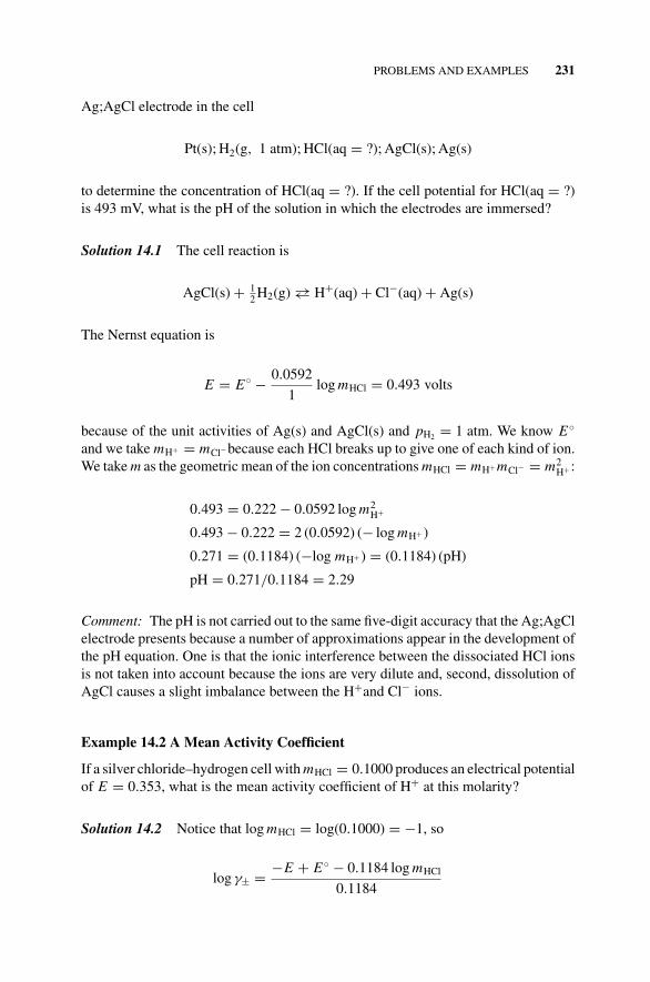
P1: OTA/XYZ P2: ABCc14 JWBS043-Rogers September 13, 2010 11:27 Printer Name: Yet to Come
PROBLEMS AND EXAMPLES 231
Ag;AgCl electrode in the cell
Pt(s); H2(g, 1 atm); HCl(aq = ?); AgCl(s); Ag(s)
to determine the concentration of HCl(aq = ?). If the cell potential for HCl(aq = ?)is 493 mV, what is the pH of the solution in which the electrodes are immersed?
Solution 14.1 The cell reaction is
AgCl(s) + 12 H2(g) →← H+(aq) + Cl−(aq) + Ag(s)
The Nernst equation is
E = E◦ − 0.0592
1log mHCl = 0.493 volts
because of the unit activities of Ag(s) and AgCl(s) and pH2 = 1 atm. We know E◦
and we take mH+ = mCl−because each HCl breaks up to give one of each kind of ion.We take m as the geometric mean of the ion concentrations mHCl = mH+mCl− = m2
H+ :
0.493 = 0.222 − 0.0592 log m2H+
0.493 − 0.222 = 2 (0.0592) (− log mH+ )
0.271 = (0.1184) (−log mH+ ) = (0.1184) (pH)
pH = 0.271/0.1184 = 2.29
Comment: The pH is not carried out to the same five-digit accuracy that the Ag;AgClelectrode presents because a number of approximations appear in the development ofthe pH equation. One is that the ionic interference between the dissociated HCl ionsis not taken into account because the ions are very dilute and, second, dissolution ofAgCl causes a slight imbalance between the H+and Cl− ions.
Example 14.2 A Mean Activity Coefficient
If a silver chloride–hydrogen cell with mHCl = 0.1000 produces an electrical potentialof E = 0.353, what is the mean activity coefficient of H+ at this molarity?
Solution 14.2 Notice that log mHCl = log(0.1000) = −1, so
log γ± = −E + E◦ − 0.1184 log mHCl
0.1184

P1: OTA/XYZ P2: ABCc14 JWBS043-Rogers September 13, 2010 11:27 Printer Name: Yet to Come
232 ELECTROCHEMICAL CELLS
m1/2
0.50.40.30.20.10.0
γ ±
0.75
0.80
0.85
0.90
0.95
1.00
FIGURE 14.3 The mean activity coefficient of HCl as a function of m1/2. The value γ± =−0.789 calculated in Exercise 14.2 is the penultimate point on the curve reading from left toright. The standard value is γ± = −0.797.
becomes
log γ± = −E + E◦ + 0.1184
0.1184= −.353 + .2224 + 0.1184
0.1184= −0.10304
γ± = −0.789
Experimental values of E at several specific values of m lead to specific values ofγ± as a function of m1/2 in Fig. 14.3. The values are less than 1.0 as predicted bythe Debye–Huckel theory. The function is not linear except at low concentrations.Experimental points deviate from the linear function.
Problem 14.1
Suppose we construct a Daniell cell (Section 14.1), conventional in every way exceptthat we replace the Zn2+(aq) and Zn(rod) with Cd2+(aq) and a Cd(s) rod.
(a) Which is the cathode and which is the anode, the copper cup or the Cd rod?
(b) What is the approximate voltage? (It is approximate because we don’t knowthe exact concentrations of the Cu(aq) and Cd(aq) solutions.)
Problem 14.2
Many applications of electrochemistry have been in chemical analysis. Supposea Zn; Zn2+ concentration cell is set up in which the Zn2+ concentration in one cell
P1: OTA/XYZ P2: ABCc14 JWBS043-Rogers September 13, 2010 11:27 Printer Name: Yet to Come
PROBLEMS AND EXAMPLES 233
compartment is 0.0100 m but the concentration of the other Zn2+ half-cell is unknown.The whole-cell potential was measured and found to be 32.4 mV.
(a) Without doing a numerical calculation, is the unknown more or less concen-trated than the 0.0100 m solution?
(b) What is the unknown concentration?
(c) Does your answer to part b agree with your answer to part a?
Problem 14.3
The half-cell (reduction) potential of the Ag:AgBr electrode is 0.071 volts. Use thisinformation with information in Section 14.3 to determine the solubility productconstant Ksp of AgBr in water.
Problem 14.4
A very important extension of electrochemical of solubility determination is gener-alization of the method to determine other kinds of equilibrium constant and fur-ther generalization to determination of the enthalpy, entropy, and Gibbs free energychanges for electrochemical reactions. Write or derive the equations for doing this.
Problem 14.5
Is it possible to reduce all of the Fe+3 ion in an aqueous solution containing Fe2+ andFe3+ by filtering the solution through finely divided Zn(s)?
Problem 14.6
What is the standard Gibbs free energy change for the preceding reaction, and doesyour answer agree with the preceding answer?
Problem 14.7
A hydrogen half-cell combined with a saturated calomel electrode has a measuredcell potential of 57.3 mV. What is the pH of the aqueous solution in the hydrogenhalf-cell? If the hydrogen electrode is a standard hydrogen electrode (SHE), what isthe cell potential?
Problem 14.8
From the cell
Pt(s); H2(g, 1 atm); HCl(aq); AgCl(s); Ag(s)
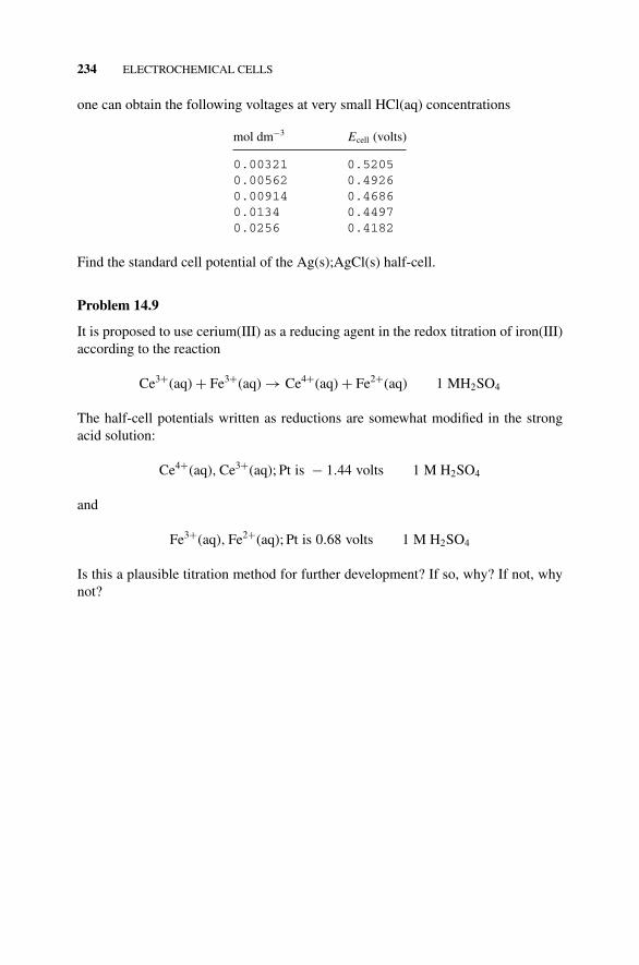
P1: OTA/XYZ P2: ABCc14 JWBS043-Rogers September 13, 2010 11:27 Printer Name: Yet to Come
234 ELECTROCHEMICAL CELLS
one can obtain the following voltages at very small HCl(aq) concentrations
mol dm−3 Ecell (volts)
0.00321 0.52050.00562 0.49260.00914 0.46860.0134 0.44970.0256 0.4182
Find the standard cell potential of the Ag(s);AgCl(s) half-cell.
Problem 14.9
It is proposed to use cerium(III) as a reducing agent in the redox titration of iron(III)according to the reaction
Ce3+(aq) + Fe3+(aq) → Ce4+(aq) + Fe2+(aq) 1 MH2SO4
The half-cell potentials written as reductions are somewhat modified in the strongacid solution:
Ce4+(aq), Ce3+(aq); Pt is − 1.44 volts 1 M H2SO4
and
Fe3+(aq), Fe2+(aq); Pt is 0.68 volts 1 M H2SO4
Is this a plausible titration method for further development? If so, why? If not, whynot?
P1: OTA/XYZ P2: ABCc15 JWBS043-Rogers September 13, 2010 11:28 Printer Name: Yet to Come
15EARLY QUANTUM THEORY:A SUMMARY
The first quarter of the twentieth century was a perplexing mix of discovery andwonderment as physicists progressed from the seemingly irrational quantization ofenergy by Max Planck (1900) to the inevitability of Werner Heisenberg’s uncertaintyprinciple (1925). For brevity, we shall refer the reader to more detailed works forthe early history of quantum theory (especially Barrow, 1996; Laidler and Meiser,1999; Atkins, 1998) and take as our starting point the observations by Louis deBroglie that small particles—in particular, electrons—have a wave nature and byErwin Schrodinger that the spectrum of atomic hydrogen can be deduced by solvingthe wave equation that now bears his name.
15.1 THE HYDROGEN SPECTRUM
Some substances give off colors in the visible region of the electromagnetic spectrumwhen excited by an energy input. An example is sodium, which glows orange when asolution of NaCl is sprayed into a flame. In general, a multiplicity of distinct energylevels within an atom leads to a corresponding multiplicity of wavelengths charac-terized by its unique electromagnetic spectrum. Distinct colors or, more specifically,wavelengths, are given off or taken up by electrons as they emit or absorb energy offrequency ν by changing levels. Emitted radiation of different wavelengths can beseparated and recorded in the form of a line spectrum. In most cases, the result of allthese energy exchanges is of bewildering complexity, but one spectrum—that of the
Concise Physical Chemistry, by Donald W. RogersCopyright C© 2011 John Wiley & Sons, Inc.
235
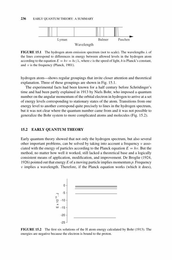
P1: OTA/XYZ P2: ABCc15 JWBS043-Rogers September 13, 2010 11:28 Printer Name: Yet to Come
236 EARLY QUANTUM THEORY: A SUMMARY
WavelengthLyman Balmer Paschen
FIGURE 15.1 The hydrogen atom emission spectrum (not to scale). The wavelengths λ ofthe lines correspond to differences in energy between allowed levels in the hydrogen atomaccording to the equation E = hν = hc/λ, where c is the speed of light, h is Planck’s constant,and ν is the frequency (Planck, 1901).
hydrogen atom—shows regular groupings that invite closer attention and theoreticalexplanation. Three of these groupings are shown in Fig. 15.1.
The experimental facts had been known for a half century before Schrodinger’stime and had been partly explained in 1913 by Niels Bohr, who imposed a quantumnumber on the angular momentum of the orbital electron in hydrogen to arrive at a setof energy levels corresponding to stationary states of the atom. Transitions from oneenergy level to another correspond quite precisely to lines in the hydrogen spectrum,but it was not clear where the quantum number came from and it was not possible togeneralize the Bohr system to more complicated atoms and molecules (Fig. 15.2).
15.2 EARLY QUANTUM THEORY
Early quantum theory showed that not only the hydrogen spectrum, but also severalother important problems, can be solved by taking into account a frequency ν asso-ciated with the energy of particles according to the Planck equation E = hν. But themethod, no matter how well it worked, still lacked a theoretical base and a logicallyconsistent means of application, modification, and improvement. De Broglie (1924,1926) pointed out that energy E of a moving particle implies momentum p. Frequencyν implies a wavelength. Therefore, if the Planck equation works (which it does),
E x
10-1
9 , J
-25
-20
-15
-10
-5
0
FIGURE 15.2 The first six solutions of the H atom energy calculated by Bohr (1913). Theenergies are negative because the electron is bound to the proton.

P1: OTA/XYZ P2: ABCc15 JWBS043-Rogers September 13, 2010 11:28 Printer Name: Yet to Come
EARLY QUANTUM THEORY 237
there should be a connection between momentum and wavelength, which he wrote asp = h/λ. At the atomic level, particles must have a wave nature. Conversely, waveshave a particle nature. This was promptly experimentally verified. This mathematicalequivalence between waves and particles is referred to as wave-particle duality.
Schrodinger (1925, 1926) reasoned that if electrons have a wavelength, they shouldfollow a wave equation. He wrote an equation for the electron in the hydrogen atomemploying a wave function �, and he arrived at the electromagnetic spectrum ofhydrogen just as Bohr had done but without making the arbitrary assumptions inherentin Bohr theory. While it should be noted that the Schrodinger equation is itself anassumption and that quantum theory is based on a set of postulates, the implicationsof Schrodinger’s theory are far wider and the results are far more general than earliertheories. Quantum mechanics now pervades virtually all of physical science frommolecular biology to string theory.
The Schrodinger equation can be written in equivalent forms with a rather in-timidating array of notations, but they are all manifestations of the same thing: thepostulate that a state vector |�〉 or state function � contains all the information wecan ever have about a mechanical system such as an atom or molecule.
The Hamiltonian function was known from classical mechanics:
E = H = T + V
where T is the kinetic energy, written in terms of the velocities v in Cartesian 3-spaceT = 1
2 m(v2
x + v2y + v2
z
), and V (x, y, z) is the potential energy. (Be careful not to
confuse velocity v with frequency ν.)An operator is a mathematical symbol telling you to do something. For example,
V tells you to multiply by the potential energy (a scalar) and ∂2/∂x2 tells you todifferentiate twice with respect to x while holding some other variable constant.(It is a partial ∂x2 because y and z are also variables.) An operator must operateon something, � in the case we are interested in. If a Hamiltonian operatorH forthe hydrogen atom system is written in terms of mathematical operators V andH = T − V in a way that is analogous to the classical Hamiltonian for the totalenergy of a conservative system, we get the operator equation
H = T + V
The Schrodinger equation is a special case of the Hamiltonian form where T isthe operator corresponding to the kinetic energy of the electron:
T = −�2
2me
(∂2
∂x2+ ∂2
∂y2+ ∂2
∂z2
)
and V (x, y, z) is the potential energy operator that describes the Coulombic attractionbetween the nucleus and the electron. (V (x, y, z) is usually written simply V (x, y, z),where we take its operator nature as obvious.)
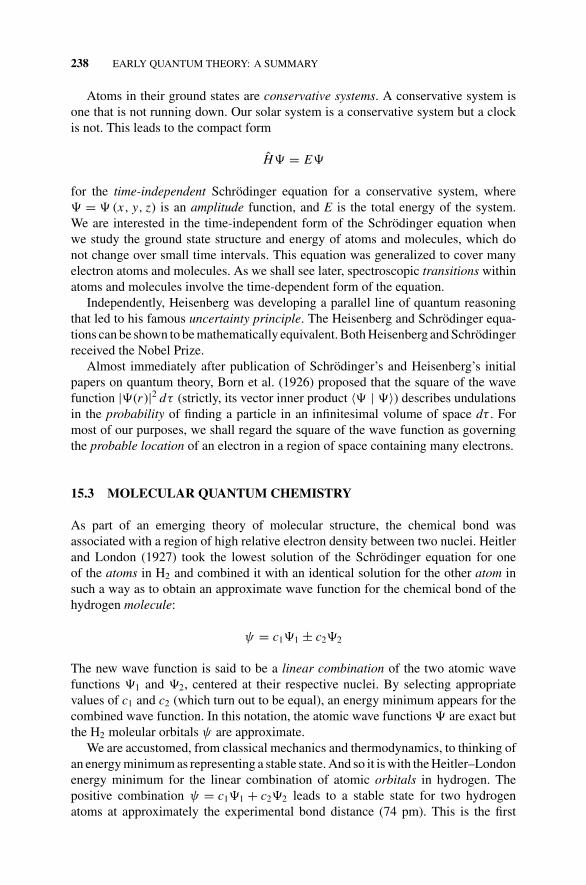
P1: OTA/XYZ P2: ABCc15 JWBS043-Rogers September 13, 2010 11:28 Printer Name: Yet to Come
238 EARLY QUANTUM THEORY: A SUMMARY
Atoms in their ground states are conservative systems. A conservative system isone that is not running down. Our solar system is a conservative system but a clockis not. This leads to the compact form
H� = E�
for the time-independent Schrodinger equation for a conservative system, where� = � (x, y, z) is an amplitude function, and E is the total energy of the system.We are interested in the time-independent form of the Schrodinger equation whenwe study the ground state structure and energy of atoms and molecules, which donot change over small time intervals. This equation was generalized to cover manyelectron atoms and molecules. As we shall see later, spectroscopic transitions withinatoms and molecules involve the time-dependent form of the equation.
Independently, Heisenberg was developing a parallel line of quantum reasoningthat led to his famous uncertainty principle. The Heisenberg and Schrodinger equa-tions can be shown to be mathematically equivalent. Both Heisenberg and Schrodingerreceived the Nobel Prize.
Almost immediately after publication of Schrodinger’s and Heisenberg’s initialpapers on quantum theory, Born et al. (1926) proposed that the square of the wavefunction |�(r )|2 dτ (strictly, its vector inner product 〈� | �〉) describes undulationsin the probability of finding a particle in an infinitesimal volume of space dτ . Formost of our purposes, we shall regard the square of the wave function as governingthe probable location of an electron in a region of space containing many electrons.
15.3 MOLECULAR QUANTUM CHEMISTRY
As part of an emerging theory of molecular structure, the chemical bond wasassociated with a region of high relative electron density between two nuclei. Heitlerand London (1927) took the lowest solution of the Schrodinger equation for oneof the atoms in H2 and combined it with an identical solution for the other atom insuch a way as to obtain an approximate wave function for the chemical bond of thehydrogen molecule:
ψ = c1�1 ± c2�2
The new wave function is said to be a linear combination of the two atomic wavefunctions �1 and �2, centered at their respective nuclei. By selecting appropriatevalues of c1 and c2 (which turn out to be equal), an energy minimum appears for thecombined wave function. In this notation, the atomic wave functions � are exact butthe H2 moleular orbitals ψ are approximate.
We are accustomed, from classical mechanics and thermodynamics, to thinking ofan energy minimum as representing a stable state. And so it is with the Heitler–Londonenergy minimum for the linear combination of atomic orbitals in hydrogen. Thepositive combination ψ = c1�1 + c2�2 leads to a stable state for two hydrogenatoms at approximately the experimental bond distance (74 pm). This is the first
P1: OTA/XYZ P2: ABCc15 JWBS043-Rogers September 13, 2010 11:28 Printer Name: Yet to Come
MOLECULAR QUANTUM CHEMISTRY 239
quantum mechanical affirmation of the two-electron bond postulated by G. N. Lewisand is familiar from general chemistry. We have the first instance of a calculatedorbital overlap leading to stability for a molecular system. The term orbital has beensubstituted for the classical mechanical term orbit in recognition of the substitutionof a probability function for a definite point location in space.
In the negative linear combination c1ψ1 − c2ψ2, we have the first example ofan antibond. The probability function for the antibond shows that electrons arerepelled from the region between the nuclei, leading to the opposite of a Lewis bond.Antibonding orbitals lie higher in energy than bonding orbitals. In some instances,infusion of energy into a molecule by incident radiation can cause electrons to bepromoted from a bonding to an antibonding orbital. Only some wavelengths areabsorbed. If the absorbed radiation is in the visible range (sunlight), we see thewavelengths left over after selective absorption as color.
Neither Schrodinger’s nor Heisenberg’s work was directed toward chemical bond-ing, so one cannot make the argument, “Well, they knew the answer before they setup the problem.” The H H bond in molecular hydrogen is a consequence of thequantum nature of matter. This point of view was developed into the valence bondtheory by Linus Pauling (1935). Much of theoretical chemistry was to be dominatedby valence bond theory (for better or for worse) for the next four decades.
Hartree (1928) is usually credited with the critical suggestion that atomic problemsinvolving many electrons can be treated as a collection of simpler problems in whicha single electron moves in an average electrostatic field created by the nucleus and allthe other electrons.1 The electrostatic attraction between a nucleus and an electron isfar greater than the energy of a chemical bond. Therefore it is reasonable to suppose, asHartree did, that one-electron wave functions would resemble Schrodinger’s solutionsfor the hydrogen atom, being identical in the angular part and differing only inthe radial probability distribution function—that is, the probable distance from thenucleus. This is the central field approximation.
Fock (1930) and Slater (1930), utilizing the prior concept of electron spin (Uhlen-beck and Goudsmit, 1925), recognized that the spin of an electron can be orientedin two ways, with or against its orbital motion. Therefore, electron spin must havea double-valued quantum number ms = ±1. A double-valued quantum number de-mands that there be two wave functions per orbital, identical in all respects exceptfor their different spins. The two wave functions must be antisymmetric just as yourright and left hands are roughly identical in shape except that they are mirror imagesof one another (antisymmetric). Two trial functions ϕ(1) and ϕ(2), having opposedspins α, and β, can combine in four ways, only one of which is antisymmetric:
ψ = ϕα(1)ϕβ(1)
ψ = ϕα(2)ϕβ(2)
ψ = ϕα(1)ϕβ(2) + ϕα(2)ϕβ(1)
ψ = ϕα(1)ϕβ(2) − ϕα(2)ϕβ(1) ←
1Hartree himself gave credit to Bohr.
P1: OTA/XYZ P2: ABCc15 JWBS043-Rogers September 13, 2010 11:28 Printer Name: Yet to Come
240 EARLY QUANTUM THEORY: A SUMMARY
The antisymmetric wave function is the same as an expanded 2 × 2 determinant:
∣∣∣∣ϕα(1) ϕβ(1)ϕα(2) ϕβ(2)
∣∣∣∣ = ϕα(1)ϕβ(2) − ϕα(2)ϕβ(1)
To impose the condition of antisymmetry on two otherwise identical orbitals, thesimple linear combinations of one-electron wave functions must be replaced by asingle-determinant wave function of the form for the two-electron case (e.g., thehelium atom):
ψ(1, 2) =∣∣∣∣ϕα(1) ϕβ(1)ϕα(2) ϕβ(2)
∣∣∣∣Generalizing to several electrons led to more complicated determinantal wavefunctions. The use of antisymmetrized orbitals, as they were called, leads to theHartree–Fock computational method. This method was applied to atoms and wastentatively applied to molecules larger than H2.
15.4 THE HARTREE INDEPENDENT ELECTRON METHOD
One can treat the electrons of a many-electron atom as though they were entirelyindependent of one another moving under the influence of the nuclear charge Z,where Z is the atomic number, an integer greater than 1. This amounts to assuminghigher-level hydrogen-like orbitals with principal quantum numbers n = Z/2 becauseeach filled orbital contains 2 independent electrons. The resulting atomic energy willbe wrong because electrons are, in fact, not independent.
This crude model can be substantially improved by taking an effective nuclearcharge smaller than Z, motivated by our intuitive understanding that, no matter whatthe overall electronic probability distribution may be, there is some probability thatsome electrons will carry a negative charge between the nucleus and the other elec-trons, thereby reducing the influence of the nuclear charge on them. Any designatedelectron will be shielded from the nuclear charge by the other electrons. Simplyplugging in arbitrary numbers for the effective nuclear charge Zeff < Z gives an im-provement in agreement of the calculated energy of the system with the experimentalvalue. It turns out that Zeff = 1.6 is a pretty good guess in the example of helium, atwo-electron problem with a nuclear charge of 2.0. Unfortunately, substitution of ar-bitrary numbers is theoretically meaningless. One would prefer to be able to calculatea radial electron probability distribution resulting in a theoretically derived energyand Zeff for any single electron from a calculated energy distribution of all the others.
In treating helium, we shall begin with the reasonable first guess that each of itstwo independent one-electron wave functions resembles that of the hydrogen atom:
� ∼= ψ1ψ2
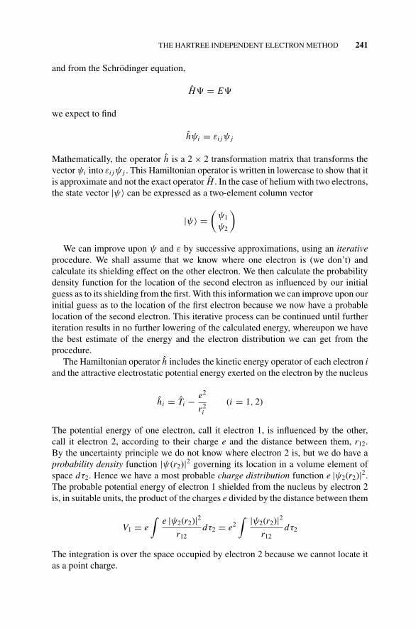
P1: OTA/XYZ P2: ABCc15 JWBS043-Rogers September 13, 2010 11:28 Printer Name: Yet to Come
THE HARTREE INDEPENDENT ELECTRON METHOD 241
and from the Schrodinger equation,
H� = E�
we expect to find
hψi = εi jψ j
Mathematically, the operator h is a 2 × 2 transformation matrix that transforms thevector ψi into εi jψ j . This Hamiltonian operator is written in lowercase to show that itis approximate and not the exact operator H . In the case of helium with two electrons,the state vector |ψ〉 can be expressed as a two-element column vector
|ψ〉 =(
ψ1
ψ2
)
We can improve upon ψ and ε by successive approximations, using an iterativeprocedure. We shall assume that we know where one electron is (we don’t) andcalculate its shielding effect on the other electron. We then calculate the probabilitydensity function for the location of the second electron as influenced by our initialguess as to its shielding from the first. With this information we can improve upon ourinitial guess as to the location of the first electron because we now have a probablelocation of the second electron. This iterative process can be continued until furtheriteration results in no further lowering of the calculated energy, whereupon we havethe best estimate of the energy and the electron distribution we can get from theprocedure.
The Hamiltonian operator h includes the kinetic energy operator of each electron iand the attractive electrostatic potential energy exerted on the electron by the nucleus
hi = Ti − e2
r2i
(i = 1, 2)
The potential energy of one electron, call it electron 1, is influenced by the other,call it electron 2, according to their charge e and the distance between them, r12.By the uncertainty principle we do not know where electron 2 is, but we do have aprobability density function |ψ(r2)|2 governing its location in a volume element ofspace dτ2. Hence we have a most probable charge distribution function e |ψ2(r2)|2.The probable potential energy of electron 1 shielded from the nucleus by electron 2is, in suitable units, the product of the charges e divided by the distance between them
V1 = e∫
e |ψ2(r2)|2r12
dτ2 = e2∫ |ψ2(r2)|2
r12dτ2
The integration is over the space occupied by electron 2 because we cannot locate itas a point charge.
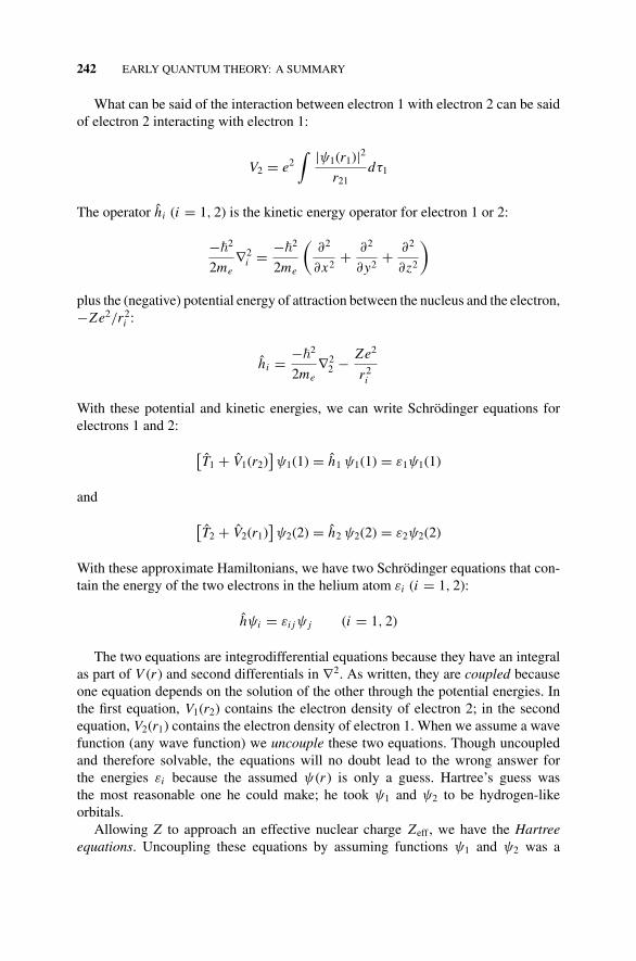
P1: OTA/XYZ P2: ABCc15 JWBS043-Rogers September 13, 2010 11:28 Printer Name: Yet to Come
242 EARLY QUANTUM THEORY: A SUMMARY
What can be said of the interaction between electron 1 with electron 2 can be saidof electron 2 interacting with electron 1:
V2 = e2∫ |ψ1(r1)|2
r21dτ1
The operator hi (i = 1, 2) is the kinetic energy operator for electron 1 or 2:
−�2
2me∇2
i = −�2
2me
(∂2
∂x2+ ∂2
∂y2+ ∂2
∂z2
)
plus the (negative) potential energy of attraction between the nucleus and the electron,−Ze2/r2
i :
hi = −�2
2me∇2
2 − Ze2
r2i
With these potential and kinetic energies, we can write Schrodinger equations forelectrons 1 and 2:
[T1 + V1(r2)
]ψ1(1) = h1 ψ1(1) = ε1ψ1(1)
and
[T2 + V2(r1)
]ψ2(2) = h2 ψ2(2) = ε2ψ2(2)
With these approximate Hamiltonians, we have two Schrodinger equations that con-tain the energy of the two electrons in the helium atom εi (i = 1, 2):
hψi = εi jψ j (i = 1, 2)
The two equations are integrodifferential equations because they have an integralas part of V (r ) and second differentials in ∇2. As written, they are coupled becauseone equation depends on the solution of the other through the potential energies. Inthe first equation, V1(r2) contains the electron density of electron 2; in the secondequation, V2(r1) contains the electron density of electron 1. When we assume a wavefunction (any wave function) we uncouple these two equations. Though uncoupledand therefore solvable, the equations will no doubt lead to the wrong answer forthe energies εi because the assumed ψ(r ) is only a guess. Hartree’s guess wasthe most reasonable one he could make; he took ψ1 and ψ2 to be hydrogen-likeorbitals.
Allowing Z to approach an effective nuclear charge Zeff , we have the Hartreeequations. Uncoupling these equations by assuming functions ψ1 and ψ2 was a
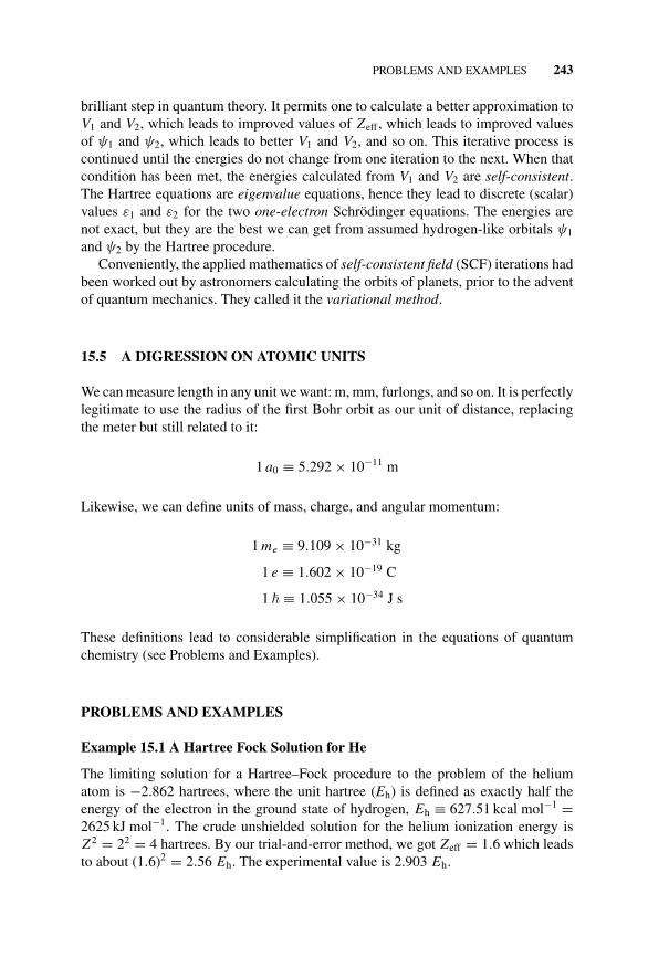
P1: OTA/XYZ P2: ABCc15 JWBS043-Rogers September 13, 2010 11:28 Printer Name: Yet to Come
PROBLEMS AND EXAMPLES 243
brilliant step in quantum theory. It permits one to calculate a better approximation toV1 and V2, which leads to improved values of Zeff , which leads to improved valuesof ψ1 and ψ2, which leads to better V1 and V2, and so on. This iterative process iscontinued until the energies do not change from one iteration to the next. When thatcondition has been met, the energies calculated from V1 and V2 are self-consistent.The Hartree equations are eigenvalue equations, hence they lead to discrete (scalar)values ε1 and ε2 for the two one-electron Schrodinger equations. The energies arenot exact, but they are the best we can get from assumed hydrogen-like orbitals ψ1
and ψ2 by the Hartree procedure.Conveniently, the applied mathematics of self-consistent field (SCF) iterations had
been worked out by astronomers calculating the orbits of planets, prior to the adventof quantum mechanics. They called it the variational method.
15.5 A DIGRESSION ON ATOMIC UNITS
We can measure length in any unit we want: m, mm, furlongs, and so on. It is perfectlylegitimate to use the radius of the first Bohr orbit as our unit of distance, replacingthe meter but still related to it:
1 a0 ≡ 5.292 × 10⁻¹¹ m
Likewise, we can define units of mass, charge, and angular momentum:
1 me ≡ 9.109 × 10⁻³¹ kg
1 e ≡ 1.602 × 10⁻¹⁹ C
1 � ≡ 1.055 × 10⁻³⁴ J s
These definitions lead to considerable simplification in the equations of quantumchemistry (see Problems and Examples).
PROBLEMS AND EXAMPLES
Example 15.1 A Hartree Fock Solution for He
The limiting solution for a Hartree–Fock procedure to the problem of the heliumatom is −2.862 hartrees, where the unit hartree (Eh) is defined as exactly half theenergy of the electron in the ground state of hydrogen, Eh ≡ 627.51 kcal mol−1 =2625 kJ mol−1. The crude unshielded solution for the helium ionization energy isZ2 = 22 = 4 hartrees. By our trial-and-error method, we got Zeff = 1.6 which leadsto about (1.6)2 = 2.56 Eh. The experimental value is 2.903 Eh.
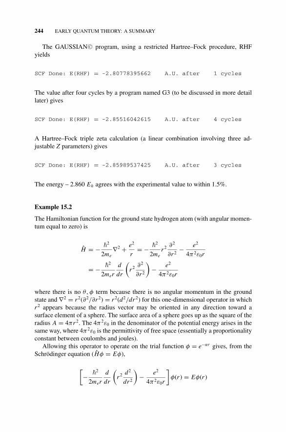
P1: OTA/XYZ P2: ABCc15 JWBS043-Rogers September 13, 2010 11:28 Printer Name: Yet to Come
244 EARLY QUANTUM THEORY: A SUMMARY
The GAUSSIAN C© program, using a restricted Hartree–Fock procedure, RHFyields
SCF Done: E(RHF) = -2.80778395662 A.U. after 1 cycles
The value after four cycles by a program named G3 (to be discussed in more detaillater) gives
SCF Done: E(RHF) = -2.85516042615 A.U. after 4 cycles
A Hartree–Fock triple zeta calculation (a linear combination involving three ad-justable Z parameters) gives
SCF Done: E(RHF) = -2.85989537425 A.U. after 3 cycles
The energy – 2.860 Eh agrees with the experimental value to within 1.5%.
Example 15.2
The Hamiltonian function for the ground state hydrogen atom (with angular momen-tum equal to zero) is
H = − �2
2me∇2 + e2
r= − �2
2mer2 ∂2
∂r2− e2
4π2ε0r
= − �2
2mer
d
dr
(r2 ∂2
∂r2
)− e2
4π2ε0r
where there is no θ, φ term because there is no angular momentum in the groundstate and ∇2 = r2(∂2/∂r2) = r2(d2/dr2) for this one-dimensional operator in whichr2 appears because the radius vector may be oriented in any direction toward asurface element of a sphere. The surface area of a sphere goes up as the square of theradius A = 4πr2. The 4π2ε0 in the denominator of the potential energy arises in thesame way, where 4π2ε0 is the permittivity of free space (essentially a proportionalityconstant between coulombs and joules).
Allowing this operator to operate on the trial function φ = e−αr gives, from theSchrodinger equation (Hφ = Eφ),
[− �2
2mer
d
dr
(r2 d2
dr2
)− e2
4π2ε0r
]φ(r ) = Eφ(r )
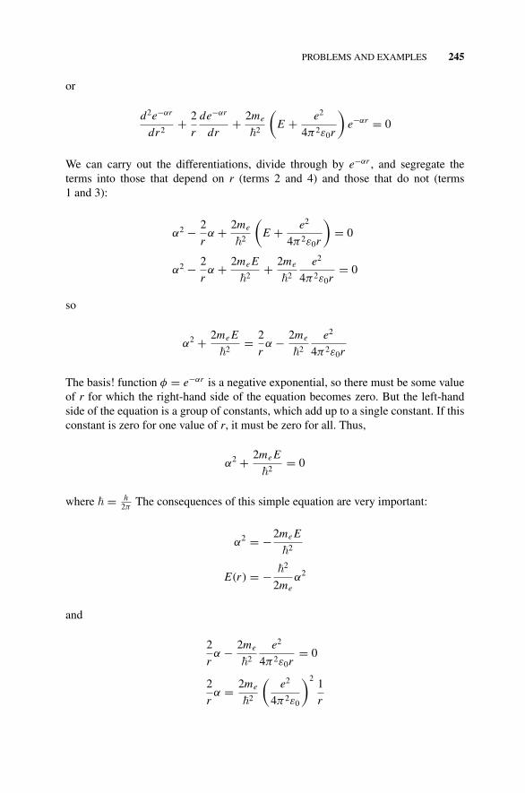
P1: OTA/XYZ P2: ABCc15 JWBS043-Rogers September 13, 2010 11:28 Printer Name: Yet to Come
PROBLEMS AND EXAMPLES 245
or
d2e−αr
dr2+ 2
r
de−αr
dr+ 2me
�2
(E + e2
4π2ε0r
)e−αr = 0
We can carry out the differentiations, divide through by e−αr , and segregate theterms into those that depend on r (terms 2 and 4) and those that do not (terms1 and 3):
α2 − 2
rα + 2me
�2
(E + e2
4π2ε0r
)= 0
α2 − 2
rα + 2me E
�2+ 2me
�2
e2
4π2ε0r= 0
so
α2 + 2me E
�2= 2
rα − 2me
�2
e2
4π2ε0r
The basis! function φ = e−αr is a negative exponential, so there must be some valueof r for which the right-hand side of the equation becomes zero. But the left-handside of the equation is a group of constants, which add up to a single constant. If thisconstant is zero for one value of r, it must be zero for all. Thus,
α2 + 2me E
�2= 0
where � = h2π
The consequences of this simple equation are very important:
α2 = −2me E
�2
E(r ) = − �2
2meα2
and
2
rα − 2me
�2
e2
4π2ε0r= 0
2
rα = 2me
�2
(e2
4π2ε0
)21
r
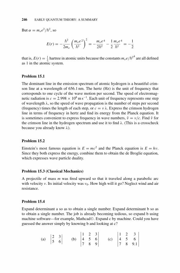
P1: OTA/XYZ P2: ABCc15 JWBS043-Rogers September 13, 2010 11:28 Printer Name: Yet to Come
246 EARLY QUANTUM THEORY: A SUMMARY
But α = mee2/�2, so
E(r ) = − �2
2me
(mee
�2
2)2
= −mee
2�2
4− 1
2
mee
�2
4= −1
2
that is, E(r ) = 12 hartree in atomic units because the constants mee/�24
are all definedas 1 in the atomic system.
Problem 15.1
The dominant line in the emission spectrum of atomic hydrogen is a beautiful crim-son line at a wavelength of 656.1 nm. The hertz (Hz) is the unit of frequency thatcorresponds to one cycle of the wave motion per second. The speed of electromag-netic radiation is c = 2.998 × 10⁸ m s−1. Each unit of frequency represents one stepof wavelength λ, so the speed of wave propagation is the number of steps per second(frequency) times the length of each step, or c = ν λ. Express the crimson hydrogenline in terms of frequency in hertz and find its energy from the Planck equation. Itis sometimes convenient to express frequency in wave numbers, ν = ν/c. Find ν forthe crimson line in the hydrogen spectrum and use it to find λ. (This is a crosscheckbecause you already know λ).
Problem 15.2
Einstein’s most famous equation is E = mc2 and the Planck equation is E = hν.Since they both express the energy, combine them to obtain the de Broglie equation,which expresses wave particle duality.
Problem 15.3 (Classical Mechanics)
A projectile of mass m was fired upward so that it traveled along a parabolic arcwith velocity v. Its initial velocity was v0. How high will it go? Neglect wind and airresistance.
Problem 15.4
Expand determinant a so as to obtain a single number. Expand determinant b so asto obtain a single number. The job is already becoming tedious, so expand b usingmachine software—for example, Mathcad C©. Expand c by machine. Could you haveguessed the answer simply by knowing b and looking at c?
(a)
∣∣∣∣ 2 35 6
∣∣∣∣ (b)
∣∣∣∣∣∣1 2 34 5 67 8 9
∣∣∣∣∣∣ (c)
∣∣∣∣∣∣1 2 34 5 67 8 9.1
∣∣∣∣∣∣
P1: OTA/XYZ P2: ABCc15 JWBS043-Rogers September 13, 2010 11:28 Printer Name: Yet to Come
PROBLEMS AND EXAMPLES 247
Problem 15.5
Good mathematical software contains a number of operations on matrices that willbe useful in coming chapters. Use Mathcad C© or similar software to calculate thesum, product, square, inversion, and product with inverse (under certain conditionsequivalent to division). Choosing matrix c from between the vertical lines in thepreceding problem enables one to solve most of these problems simply by inspectionand then allows one to verify (test run) using the software.
Problem 15.6
According to an Einstein theory of electromagnetic radiation, the 656.1-nm radiationfrom atomic hydrogen in the first excited state is a particle (later named a photon).What is the energy, frequency, wave number, and momentum of this putative particle?Express and explain the units of the final result for each of the four steps.
Problem 15.7
Show that the operator ∇2 = (1/r2)(d/dr )r2(d/dr ) in spherical coordinates canbe written ∇2 = (d2/dr2) + (2/r )(d/dr ). (This is part of the solution of the radialSchrodinger equation for the ground state of the hydrogen atom.)
Problem 15.8
Using the operator ∇2, write the radial form of the Schrodinger equation.
Problem 15.9
Allow the operator ∇2 = (d2/dr2) + (2/r )(d/dr ) to operate on the functionR(r ) = e−r in spherical polar coordinates (r, θ, and φ). What is ∇2 R(r )? What are(d R(r )/dθ ) and (d R(r )/dφ)?
P1: OTA/XYZ P2: ABCc16 JWBS043-Rogers September 13, 2010 11:28 Printer Name: Yet to Come
16WAVE MECHANICS OFSIMPLE SYSTEMS
Because of the wave nature of the electron, solution of problems of atomic andmolecular structure requires solving wave equations. Problems in atomic and molec-ular structure involve electrons that are tied to a positive nucleus or group of nucleiby electrostatic attraction. They are bound. Therefore we shall be concerned withmathematical boundary conditions imposed on the solutions of wave equations.
16.1 WAVE MOTION
Any mathematical description of a vibrating guitar string has to take into accountthe fact that it is tied down at both ends. This puts severe restrictions on the waveforms the string can take which are not characteristic of a free wave. A free wavecan assume any wavelength, but a bound wave is restricted to waves that come tozero at either end of the string. The three bound wavelengths shown in Fig. 16.1 areallowed by these two boundary conditions, but an infinite number of intermediatewavelengths are not allowed. The wave of longest wavelength is the fundamental(one observes half a sine wave), and the others are called overtones. A fundamentaland its overtones are well described by the sine function.
The wavelength λ of the first overtone is one-half the wavelength of the funda-mental λ = 1
2 λfundamental, the next overtone has λ = 13 λfundamental, and we can imagine
many overtones at λ = 1n λfundamental. This is the source of integers n that appear for
bound waves. De Broglie’s observation that particles (specifically electrons) have a
Concise Physical Chemistry, by Donald W. RogersCopyright C© 2011 John Wiley & Sons, Inc.
248
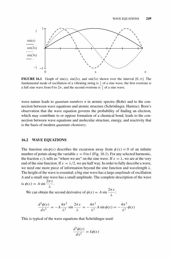
P1: OTA/XYZ P2: ABCc16 JWBS043-Rogers September 13, 2010 11:28 Printer Name: Yet to Come
WAVE EQUATIONS 249
1
11
1
sin(x)
sin(2x)
sin(3x)
x0
FIGURE 16.1 Graph of sin(x), sin(2x), and sin(3x) shown over the interval [0, π ]. Thefundamental mode of oscillation of a vibrating string is 1
2 of a sine wave, the first overtone isa full sine wave from 0 to 2π , and the second overtone is 3
2 of a sine wave.
wave nature leads to quantum numbers n in atomic spectra (Bohr) and to the con-nection between wave equations and atomic structure (Schrodinger, Hartree). Born’sobservation that the wave equation governs the probability of finding an electron,which may contribute to or oppose formation of a chemical bond, leads to the con-nection between wave equations and molecular structure, energy, and reactivity thatis the basis of modern quantum chemistry.
16.2 WAVE EQUATIONS
The function sin φ(x) describes the excursion away from φ (x) = 0 of an infinitenumber of points along the variable x = 0 to l (Fig. 16.1). For any selected harmonic,the fraction x/λ tells us “where we are” on the sine wave. If x = λ, we are at the veryend of the sine function. If x = λ/2, we are half way. In order to fully describe a wave,we need one more piece of information beyond the sine function and wavelength λ.The height of the wave is essential; a big sine wave has a large amplitude of oscillationA and a small sine wave has a small amplitude. The complete description of the wave
is φ(x) = A sin2πx
λ.
We can obtain the second derivative of φ(x) = A sin2πx
λ:
d2φ(x)
dx2= −A
4π2
λ2sin
2πx
λ= −4π2
λ2A sin φ(x) = −4π2
λ2φ(x)
This is typical of the wave equations that Schrodinger used:
d2φ(x)
dx2= kφ(x)
P1: OTA/XYZ P2: ABCc16 JWBS043-Rogers September 13, 2010 11:28 Printer Name: Yet to Come
250 WAVE MECHANICS OF SIMPLE SYSTEMS
It is also a member of the class of eigenvalue equations, in which an operator Ooperates on the eigenfunction φ(x) to give an eigenvalue k times the same function:
Oφ(x) = kφ(x)
In this case, the operator is d2/dx2, and the eigenvalue is k = −4π2/λ2.The eigenfunction may be represented as a vector:
φ(x) =(
ξ1 (x)ξ2 (x)
)
The effect of the operator is to stretch or contract the eigenvector by an amount equalto the eigenvalue, or to change its direction, or both.
Waves in two dimensions (x, y) such as those of a vibrating plate or membrane aredescribed by
∂2φ(x, y)
∂x2+ ∂2φ(x, y)
∂y2= −4π2
λ2φ(x, y)
and the wave equation in 3-space is
∂2φ(x, y, z)
∂x2+ ∂2φ(x, y, z)
∂y2+ ∂2φ(x, y, z)
∂z2= −4π2
λ2φ(x, y, z)
16.3 THE SCHRODINGER EQUATION
By the de Broglie equation p = h/λ, it follows that λ2 = h2/p2. Substituting for λ2
in a three-dimensional wave equation, we obtain
∂2φ(x, y, z)
∂x2+ ∂2φ(x, y, z)
∂y2+ ∂2φ(x, y, z)
∂z2= −4π2
λ2φ(x, y, z) = −4π2 p2
h2φ(x, y, z)
The momentum of a moving particle is its mass times its velocity,p = mv . This leadsto p2 = m2v2 = 2m( 1
2 mv2) = 2mT , where T is the classical kinetic energy 12 mv2.
Now, with a slight change in symbol for notational simplicity, we obtain
∂2�
∂x2+ ∂2�
∂y2+ ∂2�
∂z2=
(∂2
∂x2+ ∂2
∂y2+ ∂2
∂z2
)� = −8π2mT
h2�
The bracketed operator(∂2/∂x2 + ∂2/∂y2 + ∂2/∂z2
)operates on the wave function
�(x, y, z). It is given the shorthand notation ∇2. Because its eigenvalue contains a
P1: OTA/XYZ P2: ABCc16 JWBS043-Rogers September 13, 2010 11:28 Printer Name: Yet to Come
QUANTUM MECHANICAL SYSTEMS 251
group of constants times the kinetic energy T , ∇2 is called a kinetic energy operator.The total energy of a classical system is the sum of the kinetic energy and the potentialenergy, E = T + V , so the kinetic energy is the difference T = E − V and
∇2� = −8π2m
h2(E − V )�
which is one form of the famous Schrodinger equation.Other notational conveniences include the definition of “h bar,” h ≡ h/2π , which
gives
∇2� = −2m
h2 (E − V )�
and
− h2
2m∇2� + V � = E�
The kinetic energy operator plus the potential energy operator (− h2
2m ∇2� + V �)is defined as the Hamiltonian operator H by analogy to the classical Hamiltonianfunction H = T + V (Chapter 15). The kinetic and potential energy operators are Tand V , so H = T + V . (Even though V is an operator, it is often written V .) Thesenotational changes give the concise form of the Schrodinger equation:
H� = E�
where the total energy E is a scalar eigenvalue. It is distinguished from the opera-tors by not having a circumflex notation. Clearly energy is a scalar because it hasmagnitude but not direction.
16.4 QUANTUM MECHANICAL SYSTEMS
A system is a collection of mechanical entities governed by physical laws. If we knowthe state of a system, we know every physical property it can have. It is astonishingbut true that all this information can be known by specifying a very few fundamentalvariables (degrees of freedom) and a small number of postulates.
The wave function satisfies all of the properties of a vector; therefore it is writtenas a vector |�〉 or 〈�|. We shall use either the vector form |�〉 or the functional form�, according to which is more convenient. When it is useful to specify the variablesas degrees of freedom, we shall do that: |�(x1, x2, . . .)〉 or �(x1, x2, . . .), but usuallythe simpler notation |�〉 or � is preferred.
P1: OTA/XYZ P2: ABCc16 JWBS043-Rogers September 13, 2010 11:28 Printer Name: Yet to Come
252 WAVE MECHANICS OF SIMPLE SYSTEMS
One of the postulates of quantum mechanics is as follows:
If a system is in a state s described by |�〉 an eigenvector of the operator A (or,equivalently if � is an eigenfunction of A), the corresponding observable a is aneigenvalue:
A |�〉 = a |�〉
or, equivalently,
A� = a �
and experiments on s in state |�〉 will always yield the observable a.
In the case of the atomic and molecular systems that concern us here, the generaloperator A is the Hamiltonian operator, H , and the observable a is the energy levelEi of the state |�i 〉. Usually there are many states leading to many energies Ei .The set{Ei } represents a spectrum or multiplicity of energy levels, one for eacheigenvector:
H |�i 〉 = Ei |�i 〉
An operator operating on a vector produces another vector. The operator H op-erating on |�〉 produces the vector
∣∣H |� ⟩. The inner product of 〈�| premultiplied
into∣∣H |� ⟩
is
〈�| H |�〉 = 〈�| E |�〉 = E 〈� | �〉
The inner product of two vectors 〈� | �〉 is a scalar, which is why the eigenvalue Ecan be moved out of the brackets on the right. The operator H cannot be factoredout. This leads to an expression for the energy
E = 〈�| H |�〉〈� | �〉
The Born probability postulate leads to a further simplification. The inner product〈� | �〉 amounts to the integral over all space of the wave function squared �2 orthe product � ∗ � if the wave function is complex. The sum of the probabilities offinding an electron over all space must be 1.0 (certainty) because the electron hasto be somewhere. With the inner product 〈� | �〉 = 1.0 we have the energy of aneigenstate as
Ei = 〈�i | H |�i 〉
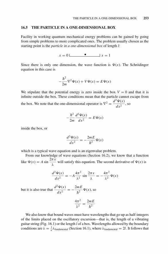
P1: OTA/XYZ P2: ABCc16 JWBS043-Rogers September 13, 2010 11:28 Printer Name: Yet to Come
THE PARTICLE IN A ONE-DIMENSIONAL BOX 253
16.5 THE PARTICLE IN A ONE-DIMENSIONAL BOX
Facility in working quantum mechanical energy problems can be gained by goingfrom simple problems to more complicated ones. The problem usually chosen as thestarting point is the particle in a one-dimensional box of length l:
x = 0 | |• x = 1
Since there is only one dimension, the wave function is �(x). The Schrodingerequation in this case is
− h2
2m∇2�(x) + V �(x) = E�(x)
We stipulate that the potential energy is zero inside the box V = 0 and that it isinfinite outside the box. These conditions mean that the particle cannot escape from
the box. We note that the one-dimensional operator is ∇2 = d2�(x)
dx2, so
− h2
2m
d2�(x)
dx2= E�(x)
inside the box, or
d2�(x)
dx2= −2m E
h2 �(x)
which is a typical wave equation and is an eigenvalue problem.From our knowledge of wave equations (Section 16.2), we know that a function
like �(x) = A sin2πx
λwill satisfy this equation. The second derivative of �(x) is
d2�(x)
dx2= −A
4π2
λ2sin
2πx
λ= −4π2
λ2�(x)
but it is also true thatd2�(x)
dx2= −2m E
h2 �(x), so
4π2
λ2= 2m E
h2
We also know that bound waves must have wavelengths that go up as half-integersof the limits placed on the oscillatory excursion—that is, the length of a vibratingguitar string (Fig. 16.1) or the length l of a box. Wavelengths allowed by the boundaryconditions are λ = 1
n λfundamental (Section 16.1), where λfundamental = 2l. It follows that
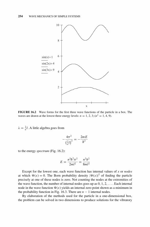
P1: OTA/XYZ P2: ABCc16 JWBS043-Rogers September 13, 2010 11:28 Printer Name: Yet to Come
254 WAVE MECHANICS OF SIMPLE SYSTEMS
2
4
6
8
10
sin(x) 1
sin(2x) 4
sin(3x) 9
x
FIGURE 16.2 Wave forms for the first three wave functions of the particle in a box. Thewaves are drawn at the lowest three energy levels: n = 1, 2, 3; (n2 = 1, 4, 9).
λ = 2n l. A little algebra goes from
− 4π2
(2n l
)2 = −2m E
h2
to the energy spectrum (Fig. 16.2):
E = n2h2π2
2ml2= n2h2
8ml2
Except for the lowest one, each wave function has internal values of x or nodesat which �(x) = 0. The Born probability density |�(x)|2 of finding the particleprecisely at one of these nodes is zero. Not counting the nodes at the extremities ofthe wave function, the number of internal nodes goes up as 0, 1, 2, . . . . Each internalnode in the wave function �(x) yields an internal zero point shown as a minimum inthe probability function in Fig. 16.3. There are n − 1 internal nodes.
By elaboration of the methods used for the particle in a one-dimensional box,the problem can be solved in two dimensions to produce solutions for the vibratory
P1: OTA/XYZ P2: ABCc16 JWBS043-Rogers September 13, 2010 11:28 Printer Name: Yet to Come
THE PARTICLE IN A CUBIC BOX 255
n 1 2 3
P n x( ) sin n x( )( )2 n2
2
4
6
8
10
P(1 x)
P(2 x)
P(3 x)
x
FIGURE 16.3 A Mathcad C© sketch of the born probability densities at the first three levelsof the particle in a box. The lowest wave function has no internal nodes, the second wavefunction has one, and the third has two.
nodes of a square plate or membrane. It can be solved in 3-space to produce solutionsto the vibratory motions in a solid cube. Other geometries are possible such as acircle, rectangle, parallelepiped, cylinder, and so on. Each problem lends insight andis recommended to the interested reader.
16.6 THE PARTICLE IN A CUBIC BOX
In the case of a particle confined to the interior of a cube, we have a three-dimensionalwave equation of the form
− h2
2m∇2�(x, y, z) + V �(x, y, z) = E�(x, y, z)
P1: OTA/XYZ P2: ABCc16 JWBS043-Rogers September 13, 2010 11:28 Printer Name: Yet to Come
256 WAVE MECHANICS OF SIMPLE SYSTEMS
We simplify this equation immediately by setting V �(x, y, z) = 0, so the middleterm drops out. The kinetic energy operator looks complicated:
− h2
2m
d2�(x, y, z)
dx2− h2
2m
d2�(x, y, z)
dy2− h2
2m
d2�(x, y, z)
dz2= E�(x, y, z)
until we make the entirely reasonable observation that, in a cube, there is no reasonto prefer particle motion in any one direction over motion in any other. The energyEx supplied by particle motion �x is the same as Ey supplied by �y and Ez suppliedby �z . This being the case, we can split one complicated equation into three simpleones:
− h2
2m
d2�(x)
dx2= Ex�(x)
− h2
2m
d2�(y)
dy2= Ey�(y)
− h2
2m
d2�(z)
dz2= Ez�(z)
Each of these equations has already been solved with the results
�(x) = A sin2πx
λ
�(y) = A sin2πy
λ
�(z) = A sin2π z
λ
and
Ex = n2x h2
8ml2
Ey = n2yh2
8ml2
Ez = n2z h2
8ml2
In the energy equations, the length of one edge of the cube l is in the denominator. If thegeometry had been other than a cube, there would be different dimensions—perhapsa, b, and c for a parallelepiped. This would have made the solutions slightly morecomplicated, but it would not have made any significant change in the result.

P1: OTA/XYZ P2: ABCc16 JWBS043-Rogers September 13, 2010 11:28 Printer Name: Yet to Come
THE PARTICLE IN A CUBIC BOX 257
x
y
z
FIGURE 16.4 The ground state orbital of a particle confined to a cubic box.
16.6.1 Orbitals
The ground state probability density has a maximum in the center when viewed fromeach of the three dimensions (Fig. 16.4). Thus there is a high probability density at thecenter of the cube diminishing symmetrically in all directions (spherical symmetry).This is the geometry of an s atomic orbital.
16.6.2 Degeneracy
If the particle is excited to the n = 2 state in the x direction while its motion in boththe y and z directions remain at the lowest energy, the resulting orbital has an internalnode in the x direction but no nodes in the y and z directions (Fig. 16.5). This givesthe geometry of the first p orbital which we denote px . What was said for the xdirection can be said for the y and z directions, so we have three orbitals with energiesthat are identical. Different orbitals with the same energy are said to be degenerate(Fig. 16.6). Perhaps we remember from elementary chemistry that the p orbitals ofhydrogen are three-fold degenerate.
16.6.3 Normalization
One can also find the constant A in �(x) = A sin2πx
λby normalizing the wave
function. Normalization requires setting the integral of �2 over all space equal to 1.0
x
y
z
FIGURE 16.5 The first excited state of a particle confined to a cubic box.
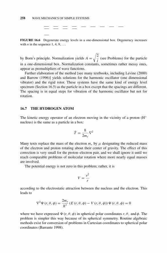
P1: OTA/XYZ P2: ABCc16 JWBS043-Rogers September 13, 2010 11:28 Printer Name: Yet to Come
258 WAVE MECHANICS OF SIMPLE SYSTEMS
FIGURE 16.6 Degenerate energy levels in a one-dimensional box. Degeneracy increaseswith n in the sequence 1, 4, 9, . . .
by Born’s principle. Normalization yields A =√
2
l(see Problems) for the particle
in a one-dimensional box. Normalization constants, sometimes rather messy ones,appear as premultipliers of wave functions.
Further elaboration of the method [see many textbooks, including Levine (2000)and Barrow (1996)] yields solutions for the harmonic oscillator (one dimensionalvibrator) and the rigid rotor. These systems have the same kind of energy levelspectrum (Section 16.5) as the particle in a box except that the spacings are different.The spacing is in equal steps for vibration of the harmonic oscillator but not forrotation.
16.7 THE HYDROGEN ATOM
The kinetic energy operator of an electron moving in the vicinity of a proton (H+
nucleus) is the same as a particle in a box:
T = h
2me∇2
Many texts replace the mass of the electron me by µ designating the reduced massof the electron and proton rotating about their center of gravity. The effect of thiscorrection is very small for the proton–electron pair, and we shall ignore it until wereach comparable problems of molecular rotation where more nearly equal massesare involved.
The potential energy is not zero in this problem; rather, it is
V = e2
r
according to the electrostatic attraction between the nucleus and the electron. Thisleads to
∇2� (r, θ, φ) = 2me
h2 (E (r, θ, φ) − V (r, θ, φ)) � (r, θ, φ) = 0
where we have expressed � (r, θ, φ) in spherical polar coordinates r, θ, and φ. Theproblem is simpler this way because of its spherical symmetry. Routine algebraicmethods exist for conversion of problems in Cartesian coordinates to spherical polarcoordinates (Barrante 1998).
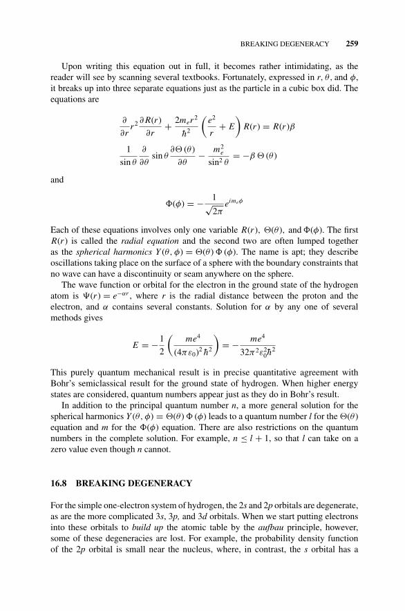
P1: OTA/XYZ P2: ABCc16 JWBS043-Rogers September 13, 2010 11:28 Printer Name: Yet to Come
BREAKING DEGENERACY 259
Upon writing this equation out in full, it becomes rather intimidating, as thereader will see by scanning several textbooks. Fortunately, expressed in r, θ, and φ,it breaks up into three separate equations just as the particle in a cubic box did. Theequations are
∂
∂rr2 ∂ R(r )
∂r+ 2mer2
h2
(e2
r+ E
)R(r ) = R(r )β
1
sin θ
∂
∂θsin θ
∂ (θ )
∂θ− m2
e
sin2 θ= −β (θ )
and
(φ) = − 1√2π
eimeφ
Each of these equations involves only one variable R(r ), (θ ), and (φ). The firstR(r ) is called the radial equation and the second two are often lumped togetheras the spherical harmonics Y (θ, φ) = (θ ) (φ). The name is apt; they describeoscillations taking place on the surface of a sphere with the boundary constraints thatno wave can have a discontinuity or seam anywhere on the sphere.
The wave function or orbital for the electron in the ground state of the hydrogenatom is �(r ) = e−αr , where r is the radial distance between the proton and theelectron, and α contains several constants. Solution for α by any one of severalmethods gives
E = −1
2
(me4
(4πε0)2 h2
)= − me4
32π2ε20h2
This purely quantum mechanical result is in precise quantitative agreement withBohr’s semiclassical result for the ground state of hydrogen. When higher energystates are considered, quantum numbers appear just as they do in Bohr’s result.
In addition to the principal quantum number n, a more general solution for thespherical harmonics Y (θ, φ) = (θ ) (φ) leads to a quantum number l for the (θ )equation and m for the (φ) equation. There are also restrictions on the quantumnumbers in the complete solution. For example, n ≤ l + 1, so that l can take on azero value even though n cannot.
16.8 BREAKING DEGENERACY
For the simple one-electron system of hydrogen, the 2s and 2p orbitals are degenerate,as are the more complicated 3s, 3p, and 3d orbitals. When we start putting electronsinto these orbitals to build up the atomic table by the aufbau principle, however,some of these degeneracies are lost. For example, the probability density functionof the 2p orbital is small near the nucleus, where, in contrast, the s orbital has a
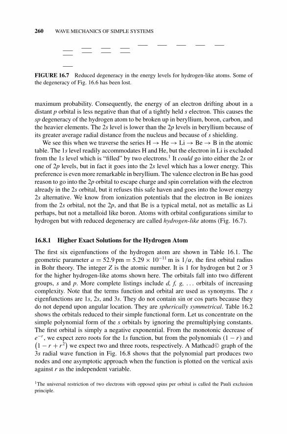
P1: OTA/XYZ P2: ABCc16 JWBS043-Rogers September 13, 2010 11:28 Printer Name: Yet to Come
260 WAVE MECHANICS OF SIMPLE SYSTEMS
FIGURE 16.7 Reduced degeneracy in the energy levels for hydrogen-like atoms. Some ofthe degeneracy of Fig. 16.6 has been lost.
maximum probability. Consequently, the energy of an electron drifting about in adistant p orbital is less negative than that of a tightly held s electron. This causes thesp degeneracy of the hydrogen atom to be broken up in beryllium, boron, carbon, andthe heavier elements. The 2s level is lower than the 2p levels in beryllium because ofits greater average radial distance from the nucleus and because of s shielding.
We see this when we traverse the series H → He → Li → Be → B in the atomictable. The 1s level readily accommodates H and He, but the electron in Li is excludedfrom the 1s level which is “filled” by two electrons.1 It could go into either the 2s orone of 2p levels, but in fact it goes into the 2s level which has a lower energy. Thispreference is even more remarkable in beryllium. The valence electron in Be has goodreason to go into the 2p orbital to escape charge and spin correlation with the electronalready in the 2s orbital, but it refuses this safe haven and goes into the lower energy2s alternative. We know from ionization potentials that the electron in Be ionizesfrom the 2s orbital, not the 2p, and that Be is a typical metal, not as metallic as Liperhaps, but not a metalloid like boron. Atoms with orbital configurations similar tohydrogen but with reduced degeneracy are called hydrogen-like atoms (Fig. 16.7).
16.8.1 Higher Exact Solutions for the Hydrogen Atom
The first six eigenfunctions of the hydrogen atom are shown in Table 16.1. Thegeometric parameter a = 52.9 pm = 5.29 × 10⁻¹¹ m is 1/α, the first orbital radiusin Bohr theory. The integer Z is the atomic number. It is 1 for hydrogen but 2 or 3for the higher hydrogen-like atoms shown here. The orbitals fall into two differentgroups, s and p. More complete listings include d, f, g, . . . orbitals of increasingcomplexity. Note that the terms function and orbital are used as synonyms. The seigenfunctions are 1s, 2s, and 3s. They do not contain sin or cos parts because theydo not depend upon angular location. They are spherically symmetrical. Table 16.2shows the orbitals reduced to their simple functional form. Let us concentrate on thesimple polynomial form of the s orbitals by ignoring the premultiplying constants.The first orbital is simply a negative exponential. From the monotonic decrease ofe−r , we expect zero roots for the 1s function, but from the polynomials (1 − r ) and(1 − r + r2
)we expect two and three roots, respectively. A Mathcad C© graph of the
3s radial wave function in Fig. 16.8 shows that the polynomial part produces twonodes and one asymptotic approach when the function is plotted on the vertical axisagainst r as the independent variable.
1The universal restriction of two electrons with opposed spins per orbital is called the Pauli exclusionprinciple.
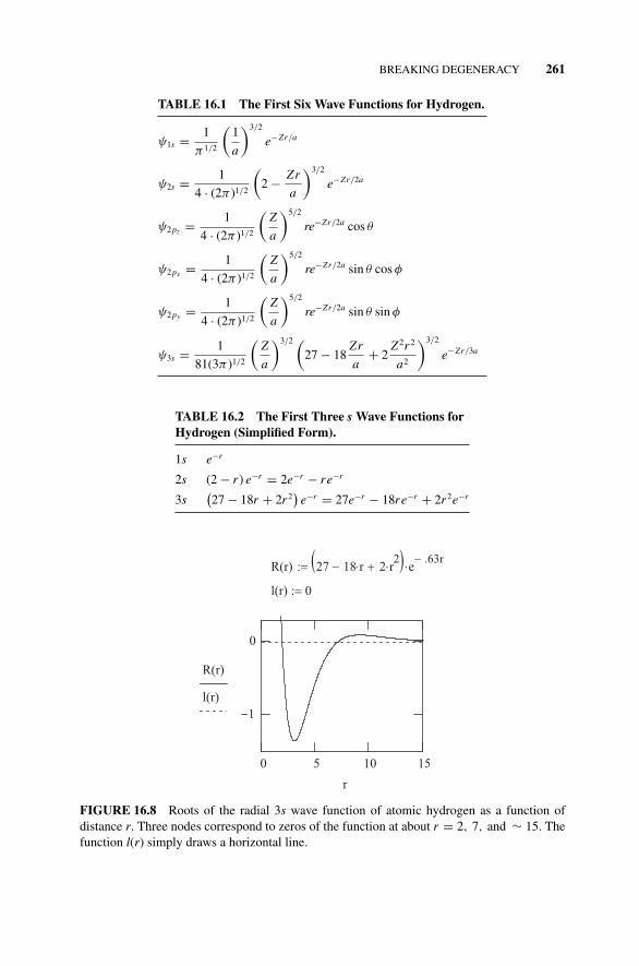
P1: OTA/XYZ P2: ABCc16 JWBS043-Rogers September 13, 2010 11:28 Printer Name: Yet to Come
BREAKING DEGENERACY 261
TABLE 16.1 The First Six Wave Functions for Hydrogen.
ψ1s = 1
π 1/2
(1
a
)3/2
e−Zr/a
ψ2s = 1
4 · (2π)1/2
(2 − Zr
a
)3/2
e−Zr/2a
ψ2pz = 1
4 · (2π)1/2
(Z
a
)5/2
re−Zr/2a cos θ
ψ2px = 1
4 · (2π)1/2
(Z
a
)5/2
re−Zr/2a sin θ cos φ
ψ2py = 1
4 · (2π)1/2
(Z
a
)5/2
re−Zr/2a sin θ sin φ
ψ3s = 1
81(3π )1/2
(Z
a
)3/2 (27 − 18
Zr
a+ 2
Z 2r 2
a2
)3/2
e−Zr/3a
TABLE 16.2 The First Three s Wave Functions forHydrogen (Simplified Form).
1s e−r
2s (2 − r ) e−r = 2e−r − re−r
3s(27 − 18r + 2r 2
)e−r = 27e−r − 18re−r + 2r 2e−r
R(r) 27 18 r r22
e.63r
l(r) 0
50 10 15
1
0
R(r)
l(r)
r
FIGURE 16.8 Roots of the radial 3s wave function of atomic hydrogen as a function ofdistance r. Three nodes correspond to zeros of the function at about r = 2, 7, and ∼ 15. Thefunction l(r) simply draws a horizontal line.
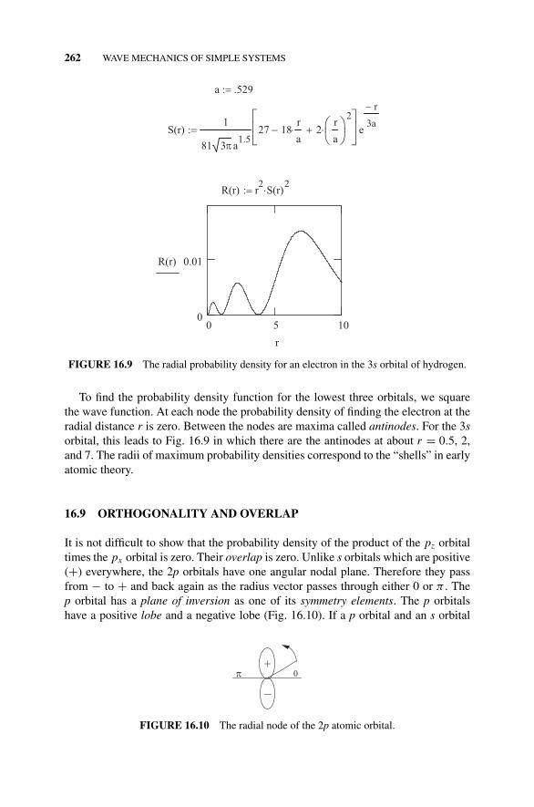
P1: OTA/XYZ P2: ABCc16 JWBS043-Rogers September 13, 2010 11:28 Printer Name: Yet to Come
262 WAVE MECHANICS OF SIMPLE SYSTEMS
a .529
S(r)1
81 3 a1.5
27 18r
a2
r
a
2
e
r
3a
R(r) r2
S(r)2
50 100
0.01R(r)
r
FIGURE 16.9 The radial probability density for an electron in the 3s orbital of hydrogen.
To find the probability density function for the lowest three orbitals, we squarethe wave function. At each node the probability density of finding the electron at theradial distance r is zero. Between the nodes are maxima called antinodes. For the 3sorbital, this leads to Fig. 16.9 in which there are the antinodes at about r = 0.5, 2,and 7. The radii of maximum probability densities correspond to the “shells” in earlyatomic theory.
16.9 ORTHOGONALITY AND OVERLAP
It is not difficult to show that the probability density of the product of the pz orbitaltimes the px orbital is zero. Their overlap is zero. Unlike s orbitals which are positive(+) everywhere, the 2p orbitals have one angular nodal plane. Therefore they passfrom − to + and back again as the radius vector passes through either 0 or π . Thep orbital has a plane of inversion as one of its symmetry elements. The p orbitalshave a positive lobe and a negative lobe (Fig. 16.10). If a p orbital and an s orbital
–
+
FIGURE 16.10 The radial node of the 2p atomic orbital.
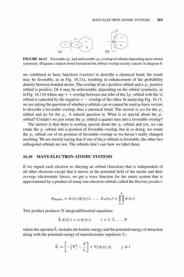
P1: OTA/XYZ P2: ABCc16 JWBS043-Rogers September 13, 2010 11:28 Printer Name: Yet to Come
MANY-ELECTRON ATOMIC SYSTEMS 263
(a)
- ++s
px
(b)-
+
pz
s
+
FIGURE 16.11 Favorable spx and unfavorable spz overlap of orbitals depending upon orbitalsymmetry. Diagram a depicts bond formation but orbital overlap exactly cancels in diagram b.
are combined as basis functions (vectors) to describe a chemical bond, the resultmay be favorable, as in Fig. 16.11a, resulting in enhancement of the probabilitydensity between bonded atoms. The overlap of an s positive orbital and a px positiveorbital is positive. Or it may be unfavorable, depending on the orbital symmetry, asin Fig. 16.11b where any + + overlap between one lobe of the 2pz orbital with the 1sorbital is canceled by the negative + − overlap of the other. In analyzing Fig. 16.11,we are asking the question of whether p orbitals can or cannot be used as basis vectorsto describe a favorable overlap, thus a chemical bond. The answer is yes for the px
orbital and no for the pz . A natural question is: What is so special about the px
orbital? Couldn’t we just rotate the pz orbital a quarter turn into a favorable overlap?The answer is that there is nothing special about the px orbital and yes, we can
rotate the pz orbital into a position of favorable overlap, but in so doing, we rotatethe px orbital out of its position of favorable overlap so we haven’t really changedanything. We are merely saying that if one of the p orbitals is favorable, the other twoorthogonal orbitals are not. The orbitals don’t care how we label them.
16.10 MANY-ELECTRON ATOMIC SYSTEMS
If we regard each electron as obeying an orbital (function) that is independent ofall other electrons except that it moves in the potential field of the nuclei and theiraverage electrostatic forces, we get a wave function for the entire system that isapproximated by a product of many one-electron orbitals called the Hartree product:
ψHartree = ψ1(r1)ψ2(r2), . . . , ψN (rN ) =N∏
i=1
ψi (ri )
This product produces N integrodifferential equations:
hiψi (ri ) = εiψi (ri ), i = 1, 2, . . . , N
where the operator hi includes the kinetic energy and the potential energy of attractionalong with the potential energy of interelectronic repulsion Vi :
hi =[− 1
2∇2i − Z
ri
]+ Vi (ψi (r j )), j �= i
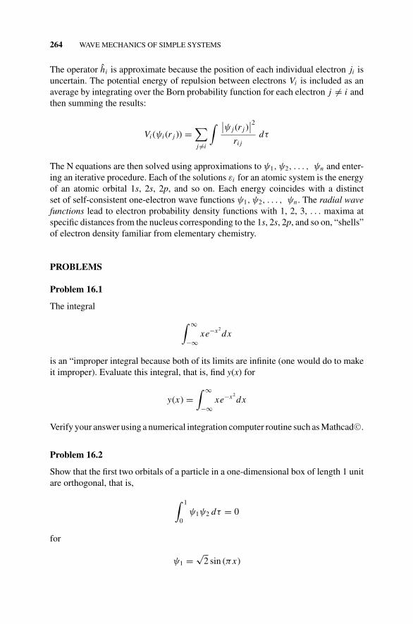
P1: OTA/XYZ P2: ABCc16 JWBS043-Rogers September 13, 2010 11:28 Printer Name: Yet to Come
264 WAVE MECHANICS OF SIMPLE SYSTEMS
The operator hi is approximate because the position of each individual electron ji isuncertain. The potential energy of repulsion between electrons Vi is included as anaverage by integrating over the Born probability function for each electron j �= i andthen summing the results:
Vi (ψi (r j )) =∑j �=i
∫ ∣∣ψ j (r j )∣∣2
ri jdτ
The N equations are then solved using approximations to ψ1, ψ2, . . . , ψn and enter-ing an iterative procedure. Each of the solutions εi for an atomic system is the energyof an atomic orbital 1s, 2s, 2p, and so on. Each energy coincides with a distinctset of self-consistent one-electron wave functions ψ1, ψ2, . . . , ψn . The radial wavefunctions lead to electron probability density functions with 1, 2, 3, . . . maxima atspecific distances from the nucleus corresponding to the 1s, 2s, 2p, and so on, “shells”of electron density familiar from elementary chemistry.
PROBLEMS
Problem 16.1
The integral
∫ ∞
−∞xe−x2
dx
is an “improper integral because both of its limits are infinite (one would do to makeit improper). Evaluate this integral, that is, find y(x) for
y(x) =∫ ∞
−∞xe−x2
dx
Verify your answer using a numerical integration computer routine such as Mathcad C©.
Problem 16.2
Show that the first two orbitals of a particle in a one-dimensional box of length 1 unitare orthogonal, that is,
∫ 1
0ψ1ψ2 dτ = 0
for
ψ1 =√
2 sin (πx)
P1: OTA/XYZ P2: ABCc16 JWBS043-Rogers September 13, 2010 11:28 Printer Name: Yet to Come
PROBLEMS 265
and
ψ2 =√
2 sin (2πx)
Problem 16.3
If the operator A = d2/dx2, find the eigenfunction φ(x) and the eigenvalue a for theeigenvalue equation
Aφ(x) = aφ(x)
Problem 16.4
According to a theory of Niels Bohr (1913) for an electron to move in a stableclassical orbit, the centrifugal force mv2/r pulling away from the nucleus must beexactly balanced by the electrostatic force of attraction between the negative electronand the positive proton e2/r2.
(a) Write an expression for the velocity of the electron.
(b) Calculate the velocity of the electron. To get your answer in SI units,use e2/4π ε0 for the charge on the electron, where 4π ε0 = 1.113 ×10⁻¹⁰ C2 s2 kg−1 m−3 is called the permittivity in a vacuum.
(c) Give units.
(d) Suppose the reader forgets to take a square root in the last step and arrives atthe result v = 4.784 × 10¹². How can he immediately know that somethinghas gone wrong?
Problem 16.5
Normalize the eigenfunction �(x) = A sin2πx
λfor the particle in a one-dimensional
box of dimension a.
Problem 16.6
Suggest a simple classical (macroscopic) mechanical system for which the probabilityfunction varies in a regular way with position. What does the probability functionlook like?
Problem 16.7
Carry out the “little algebra” to go from
− 4π2
(2n l
)2 = −2m E
h2
P1: OTA/XYZ P2: ABCc16 JWBS043-Rogers September 13, 2010 11:28 Printer Name: Yet to Come
266 WAVE MECHANICS OF SIMPLE SYSTEMS
to
E = n2h2
8m�2
Problem 16.8
What is the probability of finding an electron within one Bohr radius of the nucleusof the hydrogen atom?
Problem 16.9
The normalized wave function for a particle in a one-dimensional box of unit lengthis
�(x) =√
2 sin2πx
λ
where x tells you where you are on the excursion of the particle in the one-dimensionalx-space. What is the probability of finding a particle in the first quarter of its excursion?
P1: OTA/XYZ P2: ABCc17 JWBS043-Rogers September 13, 2010 11:28 Printer Name: Yet to Come
17THE VARIATIONAL METHOD: ATOMS
Exact orbital solutions for the hydrogen atom cannot be replicated for other atomsor molecules, even small ones, but they are of inestimable value in the mathematicaltreatment of larger systems. The energy of nuclear attraction is very much larger thanthe binding energies that dominate chemistry, so one can regard the chemical bondas a perturbation on nuclear attraction. Thus the orbitals developed for H are thefoundation stones for larger systems of ions, atoms, and the interdependent groupsof atoms that we call molecules.
17.1 MORE ON THE VARIATIONAL METHOD
A precise expression of the variational equation for approximate wavefunctions is
〈E0〉 =
∫ ∞
−∞φ∗
0 (τ )Hφ0(τ ) dτ
∫ ∞
−∞φ∗
0 (τ )φ0(τ ) dτ
In this notation, the subscripted 0 indicates the ground state energy and wave func-tions, the angle brackets around 〈E0〉 indicate an expectation value, the asterisk (∗)designates the complex conjugate of the function, and τ is a variable indicating thatthe integrals are to be taken over all space.
Concise Physical Chemistry, by Donald W. RogersCopyright C© 2011 John Wiley & Sons, Inc.
267
P1: OTA/XYZ P2: ABCc17 JWBS043-Rogers September 13, 2010 11:28 Printer Name: Yet to Come
268 THE VARIATIONAL METHOD: ATOMS
In our treatment we shall unencumber this expression from some of its notationby writing the expectation value of the energy simply as
E =
∫φ Hφ dτ∫φφ dτ
In order to evaluate this energy, we need a trial function φ, which we are free tochoose, and the Hamiltonian H , which is determined by the system.
17.2 THE SECULAR DETERMINANT
In very many cases, the wave function will not be expressed as a single function atall but as a sum of functions. To illustrate, let us take the sum of two additive terms(strictly, basis vectors in a vector space.)
φ = c1u1 + c2u2
For a variational treatment of the sum as an approximate wave function, we need theintegrals
E =
∫φ Hφ dτ∫φφ dτ
=
∫c1u1 + c2u2 Hc1u1 + c2u2 dτ∫
(c1u1 + c2u2) (c1u1 + c2u2) dτ
=c2
1
∫u1 Hu1 dτ + c1c2
∫u1 Hu2 dτ + c1c2
∫u2 Hu1 dτ + c2
2
∫u2 Hu2 dτ
c21
∫u2
1 + 2c1c2
∫u2u1 + c2
2
∫u2
2 dτ
E = c21 H11 + 2c1c2 H12 + c2 H22
c21 S11 + 2c1c2S12 + c2
2 S22
The integration problem has been broken into sums of smaller integrals. Each ofthe smaller integrals above has been given a separate symbol. The integrals in thenumerator are denoted Hi j and the integrals in the denominator are denoted Si j . Theassumption that
∫u1 Hu2 dτ =
∫u2 Hu1 dτ
P1: OTA/XYZ P2: ABCc17 JWBS043-Rogers September 13, 2010 11:28 Printer Name: Yet to Come
THE SECULAR DETERMINANT 269
has been made in order to simplify the numerator. Operators H for which this is trueare called Hermitian operators. The equivalent substitution of S12 for S21 has beenmade in the denominator.
One can multiply through by the denominator to find
(c2
1 S11 + 2c1c2S12 + c22 S22
)E = c2
1 H11 + 2c1c2 H12 + c2 H22
Our objective is to differentiate the energy with respect to each of the minimizationparameters c1 and c2 so as to find the simultaneous minimum with respect to bothof them. This will be the minimum energy obtainable from the sum of functionsφ = c1u1 + c2u2. Differentiating first with respect to c1, we obtain
(2c1S11 + 2c2S12) E + ∂ E
∂c1
(c2
1 S11 + 2c1c2S12 + c22 S22
) = 2c1 H11 + 2c2 H12
Differentiating with respect to c2, we get
(2c1S12 + 2c2S22) E + ∂ E
∂c2
(c2
1 S11 + 2c1c2S12 + c22 S22
) = 2c1 H12 + 2c2 H22
In order to find the minimum, we set
∂ E
∂c1= ∂ E
∂c2= 0
This causes the two ∂ E/∂c terms to drop out:
∂ E
∂c1
(c2
1 S11 + 2c1c2S12 + c22 S22
) = ∂ E
∂c2
(c2
1 S11 + 2c1c2S12 + c22 S22
) = 0
We are left with a pair of simultaneous equations:
(2c1S11 + 2c2S12) E = 2c1 H11 + 2c2 H12
and
(2c1S12 + 2c2S22) E = 2c1 H12 + 2c2 H22
These two equations are somewhat more conformable to computer solutions if wedivide by 2 and write them in the equivalent form:
(H11 − ES11) c1 + (H12 − ES12) c2 = 0
(H12 − ES12) c1 + (H22 − ES22) c2 = 0
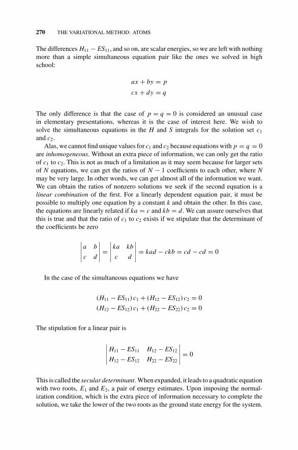
P1: OTA/XYZ P2: ABCc17 JWBS043-Rogers September 13, 2010 11:28 Printer Name: Yet to Come
270 THE VARIATIONAL METHOD: ATOMS
The differences H11 − ES11, and so on, are scalar energies, so we are left with nothingmore than a simple simultaneous equation pair like the ones we solved in highschool:
ax + by = p
cx + dy = q
The only difference is that the case of p = q = 0 is considered an unusual casein elementary presentations, whereas it is the case of interest here. We wish tosolve the simultaneous equations in the H and S integrals for the solution set c1
and c2.Alas, we cannot find unique values for c1 and c2 because equations with p = q = 0
are inhomogeneous. Without an extra piece of information, we can only get the ratioof c1 to c2. This is not as much of a limitation as it may seem because for larger setsof N equations, we can get the ratios of N − 1 coefficients to each other, where Nmay be very large. In other words, we can get almost all of the information we want.We can obtain the ratios of nonzero solutions we seek if the second equation is alinear combination of the first. For a linearly dependent equation pair, it must bepossible to multiply one equation by a constant k and obtain the other. In this case,the equations are linearly related if ka = c and kb = d. We can assure ourselves thatthis is true and that the ratio of c1 to c2 exists if we stipulate that the determinant ofthe coefficients be zero
∣∣∣∣∣a b
c d
∣∣∣∣∣ =∣∣∣∣∣ka kb
c d
∣∣∣∣∣ = kad − ckb = cd − cd = 0
In the case of the simultaneous equations we have
(H11 − ES11) c1 + (H12 − ES12) c2 = 0
(H12 − ES12) c1 + (H22 − ES22) c2 = 0
The stipulation for a linear pair is
∣∣∣∣∣H11 − ES11 H12 − ES12
H12 − ES12 H22 − ES22
∣∣∣∣∣ = 0
This is called the secular determinant. When expanded, it leads to a quadratic equationwith two roots, E1 and E2, a pair of energy estimates. Upon imposing the normal-ization condition, which is the extra piece of information necessary to complete thesolution, we take the lower of the two roots as the ground state energy for the system.
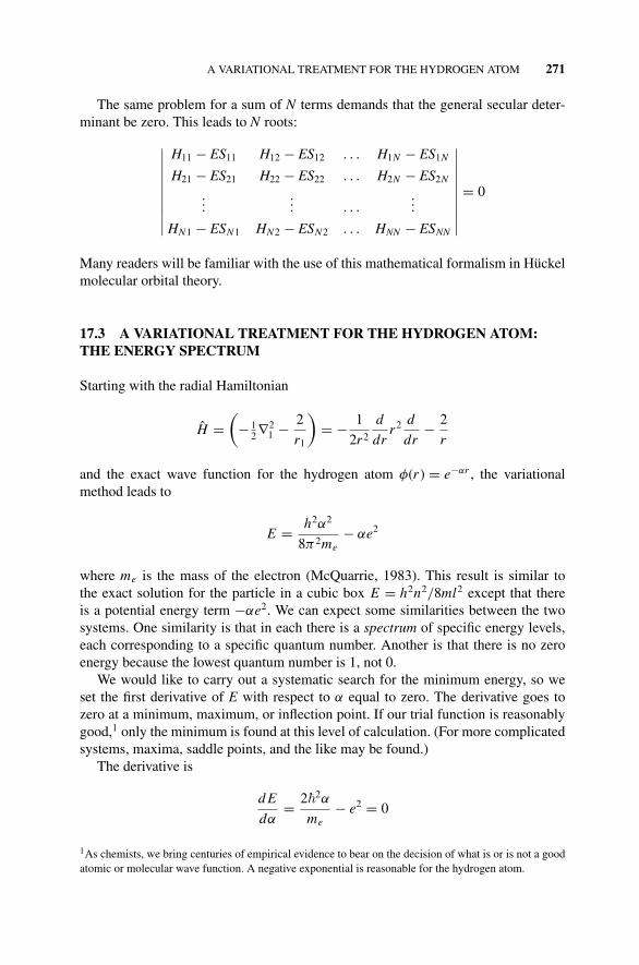
P1: OTA/XYZ P2: ABCc17 JWBS043-Rogers September 13, 2010 11:28 Printer Name: Yet to Come
A VARIATIONAL TREATMENT FOR THE HYDROGEN ATOM 271
The same problem for a sum of N terms demands that the general secular deter-minant be zero. This leads to N roots:
∣∣∣∣∣∣∣∣∣∣
H11 − ES11 H12 − ES12 . . . H1N − ES1N
H21 − ES21 H22 − ES22 . . . H2N − ES2N
...... . . .
...
HN1 − ESN1 HN2 − ESN2 . . . HNN − ESNN
∣∣∣∣∣∣∣∣∣∣= 0
Many readers will be familiar with the use of this mathematical formalism in Huckelmolecular orbital theory.
17.3 A VARIATIONAL TREATMENT FOR THE HYDROGEN ATOM:THE ENERGY SPECTRUM
Starting with the radial Hamiltonian
H =(
− 12∇2
1 − 2
r1
)= − 1
2r2
d
drr2 d
dr− 2
r
and the exact wave function for the hydrogen atom φ(r ) = e−αr , the variationalmethod leads to
E = h2α2
8π2me− αe2
where me is the mass of the electron (McQuarrie, 1983). This result is similar tothe exact solution for the particle in a cubic box E = h2n2/8ml2 except that thereis a potential energy term −αe2. We can expect some similarities between the twosystems. One similarity is that in each there is a spectrum of specific energy levels,each corresponding to a specific quantum number. Another is that there is no zeroenergy because the lowest quantum number is 1, not 0.
We would like to carry out a systematic search for the minimum energy, so weset the first derivative of E with respect to α equal to zero. The derivative goes tozero at a minimum, maximum, or inflection point. If our trial function is reasonablygood,1 only the minimum is found at this level of calculation. (For more complicatedsystems, maxima, saddle points, and the like may be found.)
The derivative is
d E
dα= 2�2α
me− e2 = 0
1As chemists, we bring centuries of empirical evidence to bear on the decision of what is or is not a goodatomic or molecular wave function. A negative exponential is reasonable for the hydrogen atom.
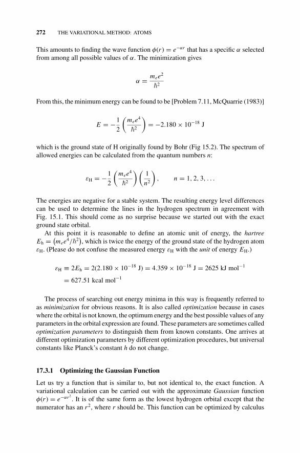
P1: OTA/XYZ P2: ABCc17 JWBS043-Rogers September 13, 2010 11:28 Printer Name: Yet to Come
272 THE VARIATIONAL METHOD: ATOMS
This amounts to finding the wave function φ(r ) = e−αr that has a specific α selectedfrom among all possible values of α. The minimization gives
α = mee2
�2
From this, the minimum energy can be found to be [Problem 7.11, McQuarrie (1983)]
E = −1
2
(mee4
�2
)= −2.180 × 10⁻¹⁸ J
which is the ground state of H originally found by Bohr (Fig 15.2). The spectrum ofallowed energies can be calculated from the quantum numbers n:
εH = −1
2
(mee4
�2
)(1
n2
), n = 1, 2, 3, . . .
The energies are negative for a stable system. The resulting energy level differencescan be used to determine the lines in the hydrogen spectrum in agreement withFig. 15.1. This should come as no surprise because we started out with the exactground state orbital.
At this point it is reasonable to define an atomic unit of energy, the hartreeEh = (
mee4/�2), which is twice the energy of the ground state of the hydrogen atom
εH. (Please do not confuse the measured energy εH with the unit of energy EH.)
εH ≡ 2Eh = 2(2.180 × 10⁻¹⁸ J) = 4.359 × 10⁻¹⁸ J = 2625 kJ mol−1
= 627.51 kcal mol−1
The process of searching out energy minima in this way is frequently referred toas minimization for obvious reasons. It is also called optimization because in caseswhere the orbital is not known, the optimum energy and the best possible values of anyparameters in the orbital expression are found. These parameters are sometimes calledoptimization parameters to distinguish them from known constants. One arrives atdifferent optimization parameters by different optimization procedures, but universalconstants like Planck’s constant h do not change.
17.3.1 Optimizing the Gaussian Function
Let us try a function that is similar to, but not identical to, the exact function. Avariational calculation can be carried out with the approximate Gaussian functionφ(r ) = e−αr2
. It is of the same form as the lowest hydrogen orbital except that thenumerator has an r2, where r should be. This function can be optimized by calculus
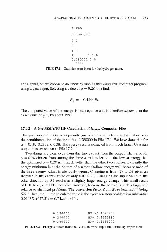
P1: OTA/XYZ P2: ABCc17 JWBS043-Rogers September 13, 2010 11:28 Printer Name: Yet to Come
A VARIATIONAL TREATMENT FOR THE HYDROGEN ATOM 273
# gen
hatom gen
0 2h
1 0S 1 1.00.280000 1.0
****
FILE 17.1 Gaussian gen input for the hydrogen atom.
and algebra, but we choose to do it now by running the Gaussian C© computer program,using a gen input. Selecting a value of α = 0.28, one finds
Eψ = − 0.4244 Eh
The computed value of the energy is less negative and is therefore higher than theexact value of 1
2 Eh by about 15%.
17.3.2 A GAUSSIAN© HF Calculation of Eatom: Computer Files
The gen keyword in Gaussian permits you to input a value for α as the first entry inthe penultimate line of the input file, 0.280000 in File 17.1. We have done this forα = 0.18, 0.28, and 0.38. The energy results extracted from much larger Gaussianoutput files are shown as File 17.2.
Two things are clear even from this tiny extract from the output. The value forα = 0.28 chosen from among the three α values leads to the lowest energy, butthe optimized α = 0.28 isn’t much better than the other two choices. Evidently theenergy minimum is at the bottom of a rather shallow energy well because none ofthe three energy values is obviously wrong. Changing α from .28 to .38 gives anincrease in the energy value of only 0.0107 Eh. Changing the input value in theother direction by 0.1 results in a slightly larger energy change. This small resultof 0.0107 Eh is a little deceptive, however, because the hartree is such a large unitrelative to chemical problems. The conversion factor from Eh to kcal mol−1 being627.51 kcal mol−1, the calculated value in the hydrogen atom problem is a substantial0.0107Eh (627.51) = 6.7 kcal mol−1.
0.180000 HF=-0.40702750.280000 HF=-0.42441320.380000 HF=-0.4136982
FILE 17.2 Energies drawn from the Gaussian gen output file for the hydrogen atom.

P1: OTA/XYZ P2: ABCc17 JWBS043-Rogers September 13, 2010 11:28 Printer Name: Yet to Come
274 THE VARIATIONAL METHOD: ATOMS
17.4 HELIUM
The helium atom is similar to the hydrogen atom, with the critical difference that thereare two electrons moving in the potential field of the nucleus. The nuclear charge is+2. The Hamiltonian for the helium atom is
H = − 12∇2
1 − 12∇2
2 − 2
r1− 2
r2+ 1
r12
Regrouping, we obtain
H =(
− 12∇2
1 − 2
r1
)+
(− 1
2∇22 − 2
r2
)+ 1
r12
The first two terms on the right replicate the hydrogen case, except for a differentnuclear charge. The third term on the right, 1/r12, is due to electrostatic repulsionof the two electrons acting over the interelectronic distance r12. This term doesnot exist in the hydrogen Hamiltonian. The sum of two nuclear and one repulsionHamiltonians is
HHe = H1 + H2 + 1
r12
If this Hamiltonian were to operate on an exact, normalized wave function for helium,the exact energy of the system would be obtained:
EHe =∫ ∞
0�(r1, r2)HHe�(r1, r2) dτ
The helium atom, however, is a three-particle system for which we cannot obtain anexact solution. The orbital and the total energy must, of necessity, be approximate.
As a naive or zero-order approximation, we can simply ignore the “r12 term” andallow the simplified Hamiltonian to operate on the 1s orbital of the H atom. Theresult is
EHe = −22
2− 22
2= − 4.00 Eh
which is 8 times the exact energy of the hydrogen atom (− 12 Eh). The 2 in the
numerators are the nuclear charge Z = 2. In general, the energy of any hydrogen-likeatom or ion is −Z2/2 hartrees per electron, provided that we ignore interelectronicelectrostatic repulsion.
We can compare this result with the first and second ionization potentials (IP) forhelium, which are energies that must go into the system to bring about ionization:
He → He++ e− → He2++ e−
P1: OTA/XYZ P2: ABCc17 JWBS043-Rogers September 13, 2010 11:28 Printer Name: Yet to Come
HELIUM 275
These energies can be measured experimentally with considerable accuracy. Sincethey are the energy necessary to pull an electron away from the helium atom, theyare equal and opposite in sign to the binding energy of the ionized electron. In thisway we have a measure of both (a) the first or “outside” electron attracted to the He+
system and (b) the inside electron attracted to the He2+ nucleus. This second energyIP2 can be calculated exactly because He+ is a one-electron (two-particle) system.The calculated second ionization potential IP2 is exactly 2.0 Eh.
If we compare the calculated total ionization potential, IP = 4.00 Eh, with theexperimental value, IP = 2.904 hartrees, the result is very bad. The magnitude of thedisaster is even more obvious if we subtract the known second ionization potential,IP2 = 2.0, from the total IP to find the first ionization potential, IP1:
IP1 = IPtotal − IP2 = 2.904 − 2.000 = 0.904 Eh
Under the approximations we have made, IP1 (calculated) = 2.000 Eh is about 110%in error. Clearly, we cannot ignore interelectronic repulsion.
17.4.1 An SCF Variational Ionization Potential for Helium
One approach to the problem of the r12 term is a variational self-consistent fieldapproximation. We shall start from Hartree’s orbital approximation, assuming thatthe orbital of helium is separable into two one-electron orbitals (1, 2) = φ1(1) φ2(2).It is reasonable to use the H atom as our starting point with the same kinetic energyoperator for each starting orbital φ1(1) and φ2(2)and −2/r as the potential energypart for attraction of each electron to a nuclear charge of 2:
H = − 1
2r2
d
drr2 d
dr− 2
r
Although we are solving for one-electron orbitals, φ1 and φ2, we do not want to fallinto the trap of the last calculation. This time we shall include a potential energy termV1 to account for the repulsion between the negative charge on the electron arbitrarilydesignated electron 1, exerted by the other electron which we shall call electron 2.
We don’t know where electron 2 is, so we must integrate over all possible locationsdτ :
V1 =∫ ∞
0φ2
1
r12φ2 dτ
The entire Hamiltonian for electron 1 is
H1 = − 1
2r21
d
dr1r2
1d
dr1− 2
r1+
∫ ∞
0φ2
1
r12φ2 dτ
P1: OTA/XYZ P2: ABCc17 JWBS043-Rogers September 13, 2010 11:28 Printer Name: Yet to Come
276 THE VARIATIONAL METHOD: ATOMS
The same treatment produces a similar operator for electron 2:
H2 = − 1
2r22
d
dr2r2
2d
dr2− 2
r2+
∫ ∞
0φ1
1
r12φ1 dτ
We do not know the orbitals of the electrons either. We can reasonably assumethat the ground state orbitals of electrons 1 and 2 are similar but not identical to the1s orbital of hydrogen:
φ1 =√
a3
πe−αr1
and
φ2 =√
b3
πe−αr2
The integral in H1, representing the Coulombic interaction between electron 1 at r1
and electron 2 somewhere in orbital φ2, has been evaluated for Slater-type orbitals(Rioux, 1987; McQuarrie, 1983) and is
V1 =∫ ∞
0φ2
1
r12φ2 dτ = 1
r1
[1 − (1 + b r1)e−2b r1
]
Now the approximate Hamiltonian for electron 1 is
h1 = − 1
2r21
d
dr1r2
1d
dr1− 2
r1+ 1
r1
(1 − (1 + br1) e−2br1
)
with a similar expression for h2 involving ar2 in place of br1 in the Slater orbital.The orbital is normalized, so the energy of electron 1 is
E1 =∫ ∞
0φ1h1 φ1 dτ
with a similar expression for E2.Calculating E1 requires solution of three integrals:
E1 =∫ ∞
0φ1
(− 12∇2
1
)φ1 dτ −
∫ ∞
0φ1
(Z
r1
)φ1 dτ +
∫ ∞
0φ1 (V1) φ1 dτ
They yield (Rioux, 1987) three terms for the energy of the electron in orbital φ1:
E1 = a2
2− Za + ab
(a2 + 3ab + b2
)(a + b)3
P1: OTA/XYZ P2: ABCc17 JWBS043-Rogers September 13, 2010 11:28 Printer Name: Yet to Come
HELIUM 277
with a similar expression for E2 except that b replaces a in the first two terms on theright
E2 = b2
2− Zb + ab
(a2 + 3ab + b2
)(a + b)3
The parameters a and b in the Slater-type orbitals for electrons 1 and 2 are min-imization parameters representing an effective nuclear charge as “experienced” byeach electron, partially shielded by the other electron from the full nuclear charge.The SCF strategy is to minimize E1 using an arbitrary starting b and to find a atthe minimum. This a value is then used to find b at the minimum E1. This valuethen replaces the starting b value and a new minimization cycle produces a newa and b, and so on until there is no progressive difference in E1. The electricalfield experienced by the electrons is now self-consistent, hence it is a self-consistentfield SCF.
In this particular case, the calculations are completely symmetrical. Everythingwe have said for a we can also say for b. At self-consistency, a = b and we cansubstitute a for b at any point in the iterative process, knowing that as we ap-proach self-consistency for one, we approach the same self-consistent value for theother.
A reasonable thing to do at the end of each iteration would be to calculatethe total energy of the atom as the sum of its two electronic energies EHe =E1 + E2, but in so doing, we would be calculating the interelectronic repulsionab(a2 + 3ab + b2)/(a + b)3 twice, once as an r12 repulsive energy and once as anr21 repulsion. The r21 repulsion should be dropped to avoid double counting, leaving
EHe = E1 + E2 = E1 + b2
2− Zb
as the correct energy of the helium atom.Although the Hartree procedure for atoms reaches self-consistency and gives a
qualitative picture of the electron probability densities, the ionization energy is still inerror by a substantial amount (0.014 h ∼= 37 kJ mol−1 on three iterations). Somethingis missing. A problem arises with the Hartree product when we exchange one atomicorbital with its adjacent neighbor
ψi (ri )ψ j (r j ) → ψ j (r j )ψi (ri )
The Hartree product is the same after exchange as it was before exchange. This isequivalent to saying that ψi (ri ) and ψ j (r j ) are identical in all respects, even thoughwe recall from elementary chemistry that no two electronic wave functions can beexactly alike and that each electron is represented by a unique set of four quantumnumbers n, l, m, and s. In three-dimensional Cartesian space, it is not difficult tosuppose that there are three quantum numbers n, l, and m in the complete solution
P1: OTA/XYZ P2: ABCc17 JWBS043-Rogers September 13, 2010 11:28 Printer Name: Yet to Come
278 THE VARIATIONAL METHOD: ATOMS
for the hydrogen atom, one for each dimension; but by using four quantum numbers,we imply something beyond the solution in 3-space.
If helium is in the excited state, the electrons are in different spatial orbitals; butin the ground state, both electrons have the same 1s orbital description. A distin-guishing fourth quantum number called the spin quantum number s = ± 1
2 must beintroduced to give two distinct 1s orbitals in helium, one designated 1sα and the otherdesignated 1sβ.
17.5 SPIN
If we ionize the electrons and examine their spins, we may find that the first electronionized (the outer electron) has spin α implying that the inner electron (2) has spin β
and that the atomic orbital �1s is
�1s = 1s(1)α + 1s(2)β
On the other hand, we may find that the first ionized electron has spin β leading to
�1s = 1s(1)β + 1s(2)α
These two results have exactly the same probability. We are in a logical dilemmathat results from the Hartree independent orbital hypothesis. It cannot be said that anelectron is in either the α spin orbital or the β spin orbital, only that they are both inan orbital that is a linear combination of equally weighted space-spin basis functions.The two plausible basis functions
1s(1)α1s(2)β and 1s(1)β1s(2)α
can be combined in two possible ways:
1s(1)α1s(2)β + 1s(1)β1s(2)α
and
1s(1)α1s(2)β − 1s(1)β1s(2)α
Only the last antisymmetrical linear combination is acceptable for the 1s electrons inhelium.
17.6 BOSONS AND FERMIONS
There are only two kinds of elementary particles in the universe, bosons and fermions.Bosons are symmetrical under exchange and fermions are antisymmetrical under

P1: OTA/XYZ P2: ABCc17 JWBS043-Rogers September 13, 2010 11:28 Printer Name: Yet to Come
SLATER DETERMINANTS 279
exchange. Electrons are fermions. If both electrons in the 1s orbital had the samespin, the negative (antisymmetric) combination above would integrate to zero andthere would be no probability of finding the electron. That is why electrons must haveopposite spins if they are to reside in the same space orbital.
17.7 SLATER DETERMINANTS
The linear combination selected above for ground state helium is the same as the ex-pansion of a 2 × 2 determinant, which is the simplest example of a Slater determinant(Section 15.3):
1s(1)α1s(2)β − 1s(1)β1s(2)α =∣∣∣∣∣1s(1)α 1s(1)β
1s(2)α 1s(2)β
∣∣∣∣∣
Larger Slater determinants also coincide with uniquely acceptable linear combina-tions for fermions. In the general n × n case with some simplification of notation,the Slater determinant is
ψ(1, 2, . . . , n) = 1√n!
∣∣∣∣∣∣∣∣∣
φ1α1 φ1β1 . . . φnα1 φnβ1
φ1α2 φ1β2 . . .
. . . . . .
φ1αn φ1βn · · · φnαn φnβn
∣∣∣∣∣∣∣∣∣
where the premultiplier 1/√
n! is a normalization constant. The many-electron wavefunction for orthonormal basis functions ψi , in more concise notation, is now written(Pople, Nobel Prize, 1998)
ψ = (n!)−12 det [(ψ1α) (ψ1β) (ψ2α) . . .]
The Slater determinant always produces a linear combination of one-electron orbitalsthat allows for electron indistinguishability by giving equal weight to electrons ofopposing spins in each of n orbitals. The Slater determinantal molecular orbitaland only the Slater determinant satisfies the two great generalizations of quantumchemistry, the Heisenberg principle of uncertainty (which is why you can’t tell inadvance whether the first electron ionized from He will be α or β) and the Fermi–Diracprinciple of antisymmetric fermion exchange.
In addition to his work on determinantal wave functions, Slater also fitted functionsto numerical compilations of SCF data and obtained orbitals in analytic form. TheseSlater-type orbitals (STO) resemble hydrogen wave functions but have adjustableparameters to account for field differences between hydrogen and many-electron
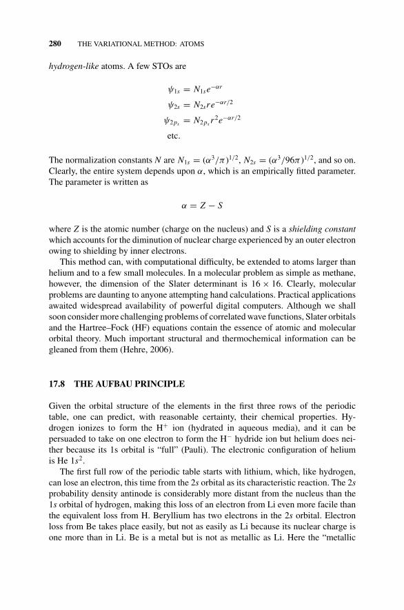
P1: OTA/XYZ P2: ABCc17 JWBS043-Rogers September 13, 2010 11:28 Printer Name: Yet to Come
280 THE VARIATIONAL METHOD: ATOMS
hydrogen-like atoms. A few STOs are
ψ1s = N1se−αr
ψ2s = N2sre−αr/2
ψ2px = N2px r2e−αr/2
etc.
The normalization constants N are N1s = (α3/π )1/2, N2s = (α3/96π )1/2, and so on.Clearly, the entire system depends upon α, which is an empirically fitted parameter.The parameter is written as
α = Z − S
where Z is the atomic number (charge on the nucleus) and S is a shielding constantwhich accounts for the diminution of nuclear charge experienced by an outer electronowing to shielding by inner electrons.
This method can, with computational difficulty, be extended to atoms larger thanhelium and to a few small molecules. In a molecular problem as simple as methane,however, the dimension of the Slater determinant is 16 × 16. Clearly, molecularproblems are daunting to anyone attempting hand calculations. Practical applicationsawaited widespread availability of powerful digital computers. Although we shallsoon consider more challenging problems of correlated wave functions, Slater orbitalsand the Hartree–Fock (HF) equations contain the essence of atomic and molecularorbital theory. Much important structural and thermochemical information can begleaned from them (Hehre, 2006).
17.8 THE AUFBAU PRINCIPLE
Given the orbital structure of the elements in the first three rows of the periodictable, one can predict, with reasonable certainty, their chemical properties. Hy-drogen ionizes to form the H+ ion (hydrated in aqueous media), and it can bepersuaded to take on one electron to form the H− hydride ion but helium does nei-ther because its 1s orbital is “full” (Pauli). The electronic configuration of heliumis He 1s2.
The first full row of the periodic table starts with lithium, which, like hydrogen,can lose an electron, this time from the 2s orbital as its characteristic reaction. The 2sprobability density antinode is considerably more distant from the nucleus than the1s orbital of hydrogen, making this loss of an electron from Li even more facile thanthe equivalent loss from H. Beryllium has two electrons in the 2s orbital. Electronloss from Be takes place easily, but not as easily as Li because its nuclear charge isone more than in Li. Be is a metal but is not as metallic as Li. Here the “metallic

P1: OTA/XYZ P2: ABCc17 JWBS043-Rogers September 13, 2010 11:28 Printer Name: Yet to Come
THE SCF ENERGIES OF FIRST-ROW ATOMS AND IONS 281
nature” of an element is defined by its tendency to lose an electron. The next sixelements—B, C, N, O, F, and Ne—correspond to the filling of the 2px , 2py , and 2pz
orbitals with two electrons each. The 3s and 3p orbitals are filled in a similar waypresenting elements that are roughly similar to their first row counterparts.
Atomic energy levels are not energetically very far apart, and one should notexpect complete regularity in the table. Small energetic perturbations cause them toshift around a bit. Sometimes the order of orbital filling, s, p, d, . . . is disrupted byexternal fields brought in by orbital interactions, ligands, solvents, or intentionallyimposed magnetic fields.
17.9 THE SCF ENERGIES OF FIRST-ROW ATOMS AND IONS
Starting from any reasonable value of a, one can calculate a value for b (Section17.4.1), substitute it as a parameter at the top of a Mathcad C© program, and repeatthe calculation to self-consistency for other small atoms. (Ignore negligibly smallimaginary roots.) Usually only three or four iterations are necessary.
The same calculation can be carried out for the single positive ions. The energydifference between the atom and its single + ion is the energy necessary to driveoff one electron, that is, the first ionization potential IP1. A collection of IP1 valuescalculated in this way is depicted in Fig. 17.1. Notice the sharp drop at Li (Z = 3),B(Z = 5), and O(Z = 8). The drop at Li results from the greater distance of theprobability antinode for 2s relative to 1s. The drop at B results from shielding of the2px orbital by the 1s2 electrons, and the drop at O results from the increased shieldingof the 2p2
x 2py2pz configuration relative to the 2px 2py2pz of N (Z = 7).
Atomic Number121086420
IP, h
artr
ees
0.1
0.2
0.3
0.4
0.5
0.6
0.7
0.8
0.9
FIGURE 17.1 Calculated IP1 for elements 1–10. Experimental results follow this pattern,but they are not identical. A more complete graph of this kind is presented in most generalchemistry texts.
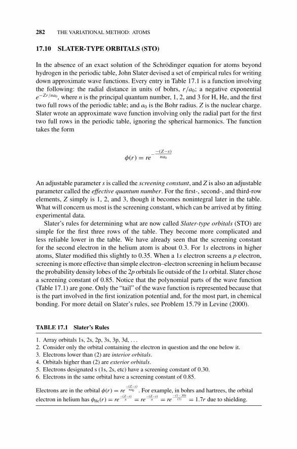
P1: OTA/XYZ P2: ABCc17 JWBS043-Rogers September 13, 2010 11:28 Printer Name: Yet to Come
282 THE VARIATIONAL METHOD: ATOMS
17.10 SLATER-TYPE ORBITALS (STO)
In the absence of an exact solution of the Schrodinger equation for atoms beyondhydrogen in the periodic table, John Slater devised a set of empirical rules for writingdown approximate wave functions. Every entry in Table 17.1 is a function involvingthe following: the radial distance in units of bohrs, r/a0; a negative exponentiale−Zr/na0 , where n is the principal quantum number, 1, 2, and 3 for H, He, and the firsttwo full rows of the periodic table; and a0 is the Bohr radius. Z is the nuclear charge.Slater wrote an approximate wave function involving only the radial part for the firsttwo full rows in the periodic table, ignoring the spherical harmonics. The functiontakes the form
φ(r ) = re− −(Z−s)
na0
An adjustable parameter s is called the screening constant, and Z is also an adjustableparameter called the effective quantum number. For the first-, second-, and third-rowelements, Z simply is 1, 2, and 3, though it becomes nonintegral later in the table.What will concern us most is the screening constant, which can be arrived at by fittingexperimental data.
Slater’s rules for determining what are now called Slater-type orbitals (STO) aresimple for the first three rows of the table. They become more complicated andless reliable lower in the table. We have already seen that the screening constantfor the second electron in the helium atom is about 0.3. For 1s electrons in higheratoms, Slater modified this slightly to 0.35. When a 1s electron screens a p electron,screening is more effective than simple electron–electron screening in helium becausethe probability density lobes of the 2p orbitals lie outside of the 1s orbital. Slater chosea screening constant of 0.85. Notice that the polynomial parts of the wave function(Table 17.1) are gone. Only the “tail” of the wave function is represented because thatis the part involved in the first ionization potential and, for the most part, in chemicalbonding. For more detail on Slater’s rules, see Problem 15.79 in Levine (2000).
TABLE 17.1 Slater’s Rules
1. Array orbitals 1s, 2s, 2p, 3s, 3p, 3d, . . .
2. Consider only the orbital containing the electron in question and the one below it.3. Electrons lower than (2) are interior orbitals.4. Orbitals higher than (2) are exterior orbitals.5. Electrons designated s (1s, 2s, etc) have a screening constant of 0.30.6. Electrons in the same orbital have a screening constant of 0.85.
Electrons are in the orbital φ(r ) = re−(Z−s)
na0 . For example, in bohrs and hartrees, the orbital
electron in helium has φHe(r ) = re−(Z−s)
n = re−(Z−s)
n = re−(1−.30)
(1) = 1.7r due to shielding.
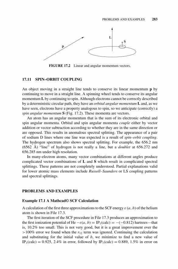
P1: OTA/XYZ P2: ABCc17 JWBS043-Rogers September 13, 2010 11:28 Printer Name: Yet to Come
PROBLEMS AND EXAMPLES 283
p
LS
FIGURE 17.2 Linear and angular momentum vectors.
17.11 SPIN–ORBIT COUPLING
An object moving in a straight line tends to conserve its linear momentum p bycontinuing to move in a straight line. A spinning wheel tends to conserve its angularmomentum L by continuing to spin. Although electrons cannot be correctly describedby a deterministic circular path, they have an orbital angular momentum L and, as wehave seen, electrons have a property analogous to spin, so we anticipate (correctly) aspin angular momentum S (Fig. 17.2). These momenta are vectors.
An atom has an angular momentum that is the sum of its electronic orbital andspin angular momenta. Orbital and spin angular momenta couple either by vectoraddition or vector subtraction according to whether they are in the same direction orare opposed. This results in anomalous spectral splitting. The appearance of a pairof sodium D lines where one line was expected is a result of spin–orbit coupling.The hydrogen spectrum also shows spectral splitting. For example, the 656.2 nm(6562 A) “line” of hydrogen is not really a line, but a doublet at 656.272 and656.285 nm under high resolution.
In many-electron atoms, many vector combinations at different angles producecomplicated vector combinations of L and S which result in complicated spectralsplittings. These patterns are not completely understood. Partial explanations validfor lower atomic mass elements include Russell–Saunders or LS coupling patternsand spectral splittings.
PROBLEMS AND EXAMPLES
Example 17.1 A Mathcad© SCF Calculation
A calculation of the first three approximations to the SCF energy ε (a, b) of the heliumatom is shown in File 17.3.
The first iteration of the SCF procedure in File 17.3 produces an approximation tothe first ionization potential of He −ε(a, b) = IP1(calc) = −(−0.812) hartrees—thatis, 10.2% too small. This is not very good, but it is a great improvement over the>100% error we found when the r12 term was ignored. Continuing the calculationand substituting for the initial value of b, we minimize to find a new value ofIP1(calc) = 0.925, 2.4% in error, followed by IP1(calc) = 0.889, 1.5% in error on
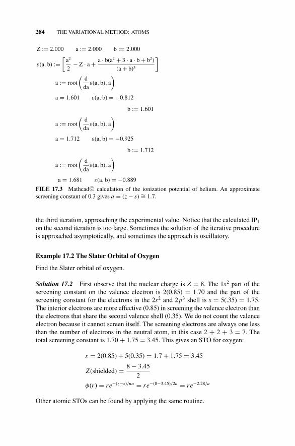
P1: OTA/XYZ P2: ABCc17 JWBS043-Rogers September 13, 2010 11:28 Printer Name: Yet to Come
284 THE VARIATIONAL METHOD: ATOMS
Z := 2.000 a := 2.000 b := 2.000
ε(a, b) :=[
a2
2− Z · a + a · b(a2 + 3 · a · b + b2)
(a + b)3
]
a := root
(d
daε(a, b), a
)
a = 1.601 ε(a, b) = −0.812
b := 1.601
a := root
(d
daε(a, b), a
)
a = 1.712 ε(a, b) = −0.925
b := 1.712
a := root
(d
daε(a, b), a
)
a = 1.681 ε(a, b) = −0.889
FILE 17.3 Mathcad C© calculation of the ionization potential of helium. An approximatescreening constant of 0.3 gives a = (z − s) ∼= 1.7.
the third iteration, approaching the experimental value. Notice that the calculated IP1
on the second iteration is too large. Sometimes the solution of the iterative procedureis approached asymptotically, and sometimes the approach is oscillatory.
Example 17.2 The Slater Orbital of Oxygen
Find the Slater orbital of oxygen.
Solution 17.2 First observe that the nuclear charge is Z = 8. The 1s2 part of thescreening constant on the valence electron is 2(0.85) = 1.70 and the part of thescreening constant for the electrons in the 2s2 and 2p3 shell is s = 5(.35) = 1.75.The interior electrons are more effective (0.85) in screening the valence electron thanthe electrons that share the second valence shell (0.35). We do not count the valenceelectron because it cannot screen itself. The screening electrons are always one lessthan the number of electrons in the neutral atom, in this case 2 + 2 + 3 = 7. Thetotal screening constant is 1.70 + 1.75 = 3.45. This gives an STO for oxygen:
s = 2(0.85) + 5(0.35) = 1.7 + 1.75 = 3.45
Z (shielded) = 8 − 3.45
2
φ(r ) = re−(z−s)/na = re−(8−3.45)/2a = re−2.28/a
Other atomic STOs can be found by applying the same routine.
P1: OTA/XYZ P2: ABCc17 JWBS043-Rogers September 13, 2010 11:28 Printer Name: Yet to Come
PROBLEMS AND EXAMPLES 285
Problem 17.1
Evaluate the following determinants:
∣∣∣∣∣1 0
0 1
∣∣∣∣∣ ,∣∣∣∣∣
x 1
1 x
∣∣∣∣∣ ,∣∣∣∣∣
sin θ cos θ
− cos θ sin θ
∣∣∣∣∣
Problem 17.2
What is the energy increase relative to the ground state when one of the quantumnumbers, say nz , for the particle in a cubic box is raised from 1 to 2? What is thedegeneracy of the resulting wave function and probability distribution?
Problem 17.3
1,3-Pentadiene shows a strong absorption peak at 45,000 cm−1 (Ege, 1994). Whatis the wavelength of this radiation in (a) centimeters, (b) meters, (c) nanometers,(d) picometers, and (e) angstroms? What is its frequency in hertz? What is its energyin joules?
Problem 17.4
What is the actual energy increase for the single excitation nz = 1 → nz = 2 inProblem 17.2 if the trapped particle is an electron and the dimension of the box isapproximately a bond length, 1.5 A? Give your answer in joules. What wavelength oflight will promote an electron from the ground state to one of the degenerate excitedstates? Give your answer in nanometers.
Problem 17.5
The length of an ethene molecule is about 153 pm according to MM3. Using Huckeltheory and the particle in a one-dimensional box as a model, in what region ofthe electromagnetic spectrum (X-ray, UV, vis, IR, etc.) is the radiation necessary topromote an electron from the highest occupied molecular orbital (HOMO) to thelowest unoccupied molecular orbital (LUMO)?
Problem 17.6
Find the Slater-type orbital (STO) of nitrogen.
Problem 17.7
Write down the unnormalized Slater determinant for He in the ground state. The Heatom is a three-particle, two-electron system. Set the Slater determinant, including a
P1: OTA/XYZ P2: ABCc17 JWBS043-Rogers September 13, 2010 11:28 Printer Name: Yet to Come
286 THE VARIATIONAL METHOD: ATOMS
normalization constant, equal to the wave function of He. Expand the determinant.What is the normalization constant?
Problem 17.8
We have seen that the linear combination that is the difference between terms isequivalent to the Slater determinantal wave function for helium.
ψHe(1, 2) = 1√n
(1s(1)α(1)1s(2)β(2) − 1s(2)α(2)1s(1)β(1))
≡ 1√n
∣∣∣∣∣1s(1)α(1) 1s(1)β(1)
1s(2)α(2) 1s(2)β(2)
∣∣∣∣∣What is wrong with the positive combination?
ψHe(1, 2)1√n
(1s(1)α(1)1s(2)β(2) + 1s(2)α(2)1s(1)β(1))
Hint: Try switching electrons ψHe(1, 2) → ψHe(2, 1).
Problem 17.9
A variational treatment of atomic helium gave
EHe = −(−2Z2eff + 5
4Zeff + 4Zeff(Zeff − 2))EH
Find Zeff and EHe given that EH = −13.6 eV. Give your answer also in electron volts.The experimental result is EHe = −79.0 eV. What is the % error of this variationaltreatment?
P1: OTA/XYZ P2: ABCc18 JWBS043-Rogers September 13, 2010 11:29 Printer Name: Yet to Come
18EXPERIMENTAL DETERMINATIONOF MOLECULAR STRUCTURE
Acceptance, at least provisional acceptance, of atomic theory goes back two anda half millennia, but it inevitably raises the question of what atoms look like. Thenature of the world around us—air, earth, fire, and water—is governed less by atomicproperties than by the physical and chemical properties of molecules. But acceptanceof molecular theory, a child of the nineteenth century, raises the same question:What do molecules look like? Experimental evidence for the existence and physicalappearance of molecules comes from interactions of confined pure samples with theirenvironment, largely through energy transfer by the very broad energy spectrum ofelectromagnetic radiation extending all the way from gamma and X rays to low-energy radio waves.
18.1 THE HARMONIC OSCILLATOR
A mass attached to a fixed beam by a spring can be set into oscillation by pullingit down and letting it go (Fig. 18.1). An ordinary spring obeys Hooke’s law, at leastapproximately:
f = −k f z(t)
where f is the force exerted by the spring on the moving mass when it is displacedby a distance z from the equilibrium distance z0. The proportionality constant k f is
Concise Physical Chemistry, by Donald W. RogersCopyright C© 2011 John Wiley & Sons, Inc.
287
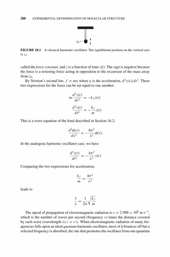
P1: OTA/XYZ P2: ABCc18 JWBS043-Rogers September 13, 2010 11:29 Printer Name: Yet to Come
288 EXPERIMENTAL DETERMINATION OF MOLECULAR STRUCTURE
z0
FIGURE 18.1 A classical harmonic oscillator. The equilibrium position on the vertical axisis z0.
called the force constant, and z is a function of time z(t). The sign is negative becausethe force is a restoring force acting in opposition to the excursion of the mass awayfrom z0.
By Newton’s second law, f = ma where a is the acceleration, d2z(t)/dt2. Thesetwo expressions for the force can be set equal to one another:
md2z(t)
dt2= −k f z(t)
d2z(t)
dt2= −k f
mz(t)
This is a wave equation of the kind described in Section 16.2:
d2φ(x)
dx2= −4π2
λ2φ(x)
In the analogous harmonic oscillator case, we have
d2z(t)
dt2= −4π2
λ2z(t)
Comparing the two expressions for acceleration,
k f
m= 4π2
λ2
leads to
1
λ= 1
2π
√k f
m
The speed of propagation of electromagnetic radiation is c = 2.998 × 10⁸ m s−1,which is the number of waves per second (frequency ν) times the distance coveredby each wave (wavelength λ) c = ν λ. When electromagnetic radiation of many fre-quencies falls upon an ideal quantum harmonic oscillator, most of it bounces off but aselected frequency is absorbed, the one that promotes the oscillator from one quantum
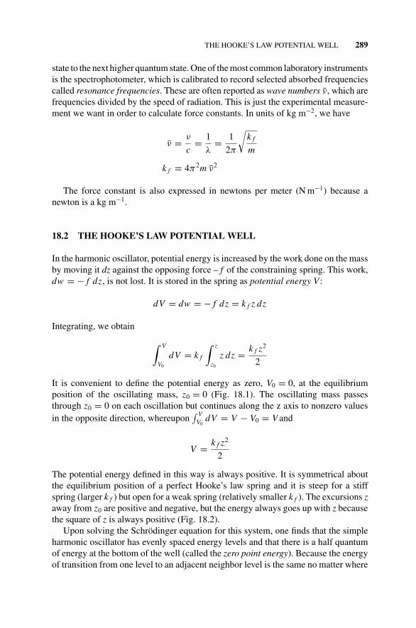
P1: OTA/XYZ P2: ABCc18 JWBS043-Rogers September 13, 2010 11:29 Printer Name: Yet to Come
THE HOOKE’S LAW POTENTIAL WELL 289
state to the next higher quantum state. One of the most common laboratory instrumentsis the spectrophotometer, which is calibrated to record selected absorbed frequenciescalled resonance frequencies. These are often reported as wave numbers ν, which arefrequencies divided by the speed of radiation. This is just the experimental measure-ment we want in order to calculate force constants. In units of kg m−2, we have
ν = ν
c= 1
λ= 1
2π
√k f
m
k f = 4π2m ν2
The force constant is also expressed in newtons per meter (N m−1) because anewton is a kg m−1.
18.2 THE HOOKE’S LAW POTENTIAL WELL
In the harmonic oscillator, potential energy is increased by the work done on the massby moving it dz against the opposing force – f of the constraining spring. This work,dw = − f dz, is not lost. It is stored in the spring as potential energy V:
dV = dw = − f dz = k f z dz
Integrating, we obtain
∫ V
V0
dV = k f
∫ z
z0
z dz = k f z2
2
It is convenient to define the potential energy as zero, V0 = 0, at the equilibriumposition of the oscillating mass, z0 = 0 (Fig. 18.1). The oscillating mass passesthrough z0 = 0 on each oscillation but continues along the z axis to nonzero valuesin the opposite direction, whereupon
∫ VV0
dV = V − V0 = V and
V = k f z2
2
The potential energy defined in this way is always positive. It is symmetrical aboutthe equilibrium position of a perfect Hooke’s law spring and it is steep for a stiffspring (larger k f ) but open for a weak spring (relatively smaller k f ). The excursions zaway from z0 are positive and negative, but the energy always goes up with z becausethe square of z is always positive (Fig. 18.2).
Upon solving the Schrodinger equation for this system, one finds that the simpleharmonic oscillator has evenly spaced energy levels and that there is a half quantumof energy at the bottom of the well (called the zero point energy). Because the energyof transition from one level to an adjacent neighbor level is the same no matter where

P1: OTA/XYZ P2: ABCc18 JWBS043-Rogers September 13, 2010 11:29 Printer Name: Yet to Come
290 EXPERIMENTAL DETERMINATION OF MOLECULAR STRUCTURE
V
zz0
FIGURE 18.2 Parabolic potential wells for the harmonic oscillator. The narrow well has thelarger force constant. Only one set of quantum levels is shown.
you start, the absorption spectrum for the harmonic oscillator consists of only oneline with frequency ν = (�E/h) s−1 because �E = h ν.
The simple harmonic oscillator is a fairly good model for a hydrogen atom sus-pended from a heavy carbon atom framework (Fig. 18.1). From C–H resonancefrequencies of about 2900–3000 cm−1, one finds the force constant to be about500 N m−1. Typical experimental values for molecular force constants vary consid-erably, from about 100 N m−1 to about 800 N m−1.
The reader with practical knowledge of infrared spectra will find a discrepancybetween the complicated structure of a real IR band spectrum and the single linepredicted by Hooke’s law. This is the result of many factors, including the failureof Hooke’s law, energy coupling among chemical bonds, and many other motions(bending, torsion, etc.) that are possible in a real polyatomic molecule. Nevertheless,the presence of a strong peak near 2900–3000 cm−1 is a good indicator of a C–Hstretch lurking somewhere in the molecule. Other characteristic frequencies are usedin qualitative IR “fingerprint” analysis.
18.3 DIATOMIC MOLECULES
For diatomic molecules attached by a chemical bond, the picture is very similar tothe harmonic oscillator of one mass. The atoms vibrate harmonically relative to oneanother with a natural frequency determined by their mass and the strength of theelectronic spring connecting them. One replaces the mass of the simple harmonicoscillator with the reduced mass of the diatomic molecule µ = m1m2/m1 + m2,where m1 and m2 are the atomic masses, and proceeds with the calculation. Theproblem has indeed been reduced from one of two masses vibrating relative to oneanother to one of a single fictitious mass µ vibrating relative to a central point.
18.4 THE QUANTUM RIGID ROTOR
A small mass on a circular orbit in a fixed plane shows quantum phenomena. Theenergy level spacing shows a pattern that is similar to the energy levels of the particle
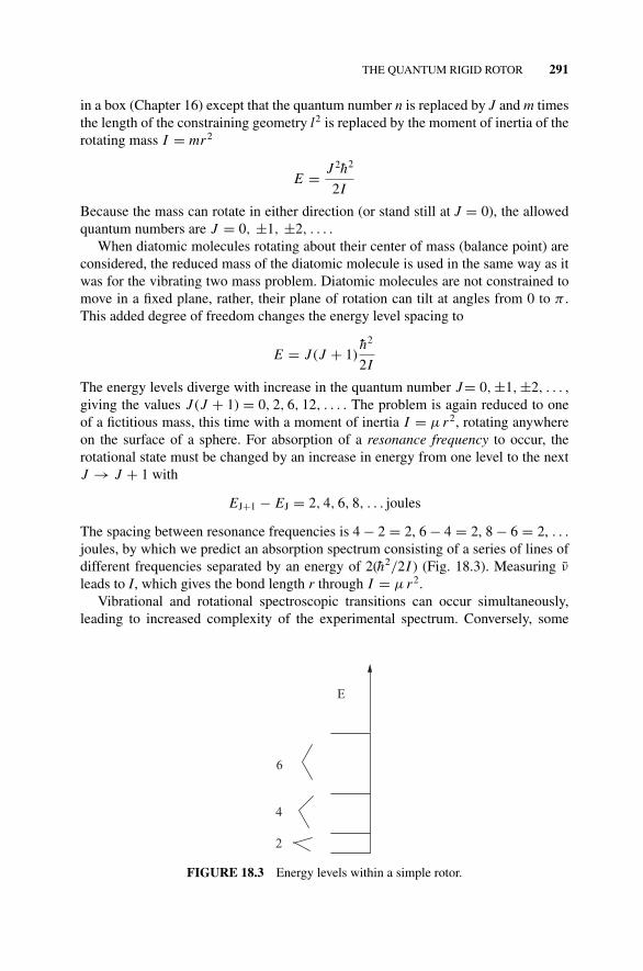
P1: OTA/XYZ P2: ABCc18 JWBS043-Rogers September 13, 2010 11:29 Printer Name: Yet to Come
THE QUANTUM RIGID ROTOR 291
in a box (Chapter 16) except that the quantum number n is replaced by J and m timesthe length of the constraining geometry l2 is replaced by the moment of inertia of therotating mass I = mr2
E = J 2h2
2I
Because the mass can rotate in either direction (or stand still at J = 0), the allowedquantum numbers are J = 0, ±1, ±2, . . . .
When diatomic molecules rotating about their center of mass (balance point) areconsidered, the reduced mass of the diatomic molecule is used in the same way as itwas for the vibrating two mass problem. Diatomic molecules are not constrained tomove in a fixed plane, rather, their plane of rotation can tilt at angles from 0 to π .This added degree of freedom changes the energy level spacing to
E = J (J + 1)h2
2I
The energy levels diverge with increase in the quantum number J= 0,±1,±2, . . . ,giving the values J (J + 1) = 0, 2, 6, 12, . . . . The problem is again reduced to oneof a fictitious mass, this time with a moment of inertia I = µ r2, rotating anywhereon the surface of a sphere. For absorption of a resonance frequency to occur, therotational state must be changed by an increase in energy from one level to the nextJ → J + 1 with
EJ+1 − EJ = 2, 4, 6, 8, . . . joules
The spacing between resonance frequencies is 4 − 2 = 2, 6 − 4 = 2, 8 − 6 = 2, . . .
joules, by which we predict an absorption spectrum consisting of a series of lines ofdifferent frequencies separated by an energy of 2(h2/2I ) (Fig. 18.3). Measuring ν
leads to I, which gives the bond length r through I = µ r2.Vibrational and rotational spectroscopic transitions can occur simultaneously,
leading to increased complexity of the experimental spectrum. Conversely, some
2
4
6
E
FIGURE 18.3 Energy levels within a simple rotor.
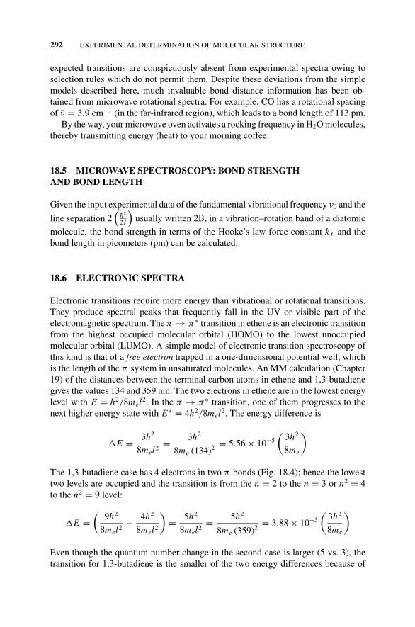
P1: OTA/XYZ P2: ABCc18 JWBS043-Rogers September 13, 2010 11:29 Printer Name: Yet to Come
292 EXPERIMENTAL DETERMINATION OF MOLECULAR STRUCTURE
expected transitions are conspicuously absent from experimental spectra owing toselection rules which do not permit them. Despite these deviations from the simplemodels described here, much invaluable bond distance information has been ob-tained from microwave rotational spectra. For example, CO has a rotational spacingof ν = 3.9 cm−1 (in the far-infrared region), which leads to a bond length of 113 pm.
By the way, your microwave oven activates a rocking frequency in H2O molecules,thereby transmitting energy (heat) to your morning coffee.
18.5 MICROWAVE SPECTROSCOPY: BOND STRENGTHAND BOND LENGTH
Given the input experimental data of the fundamental vibrational frequency ν0 and the
line separation 2(
h2
2I
)usually written 2B, in a vibration–rotation band of a diatomic
molecule, the bond strength in terms of the Hooke’s law force constant k f and thebond length in picometers (pm) can be calculated.
18.6 ELECTRONIC SPECTRA
Electronic transitions require more energy than vibrational or rotational transitions.They produce spectral peaks that frequently fall in the UV or visible part of theelectromagnetic spectrum. The π → π∗ transition in ethene is an electronic transitionfrom the highest occupied molecular orbital (HOMO) to the lowest unoccupiedmolecular orbital (LUMO). A simple model of electronic transition spectroscopy ofthis kind is that of a free electron trapped in a one-dimensional potential well, whichis the length of the π system in unsaturated molecules. An MM calculation (Chapter19) of the distances between the terminal carbon atoms in ethene and 1,3-butadienegives the values 134 and 359 nm. The two electrons in ethene are in the lowest energylevel with E = h2/8mel2. In the π → π∗ transition, one of them progresses to thenext higher energy state with E∗ = 4h2/8mel2. The energy difference is
�E = 3h2
8mel2= 3h2
8me (134)2 = 5.56 × 10⁻⁵
(3h2
8me
)
The 1,3-butadiene case has 4 electrons in two π bonds (Fig. 18.4); hence the lowesttwo levels are occupied and the transition is from the n = 2 to the n = 3 or n2 = 4to the n2 = 9 level:
�E =(
9h2
8mel2− 4h2
8mel2
)= 5h2
8mel2= 5h2
8me (359)2 = 3.88 × 10⁻⁵
(3h2
8me
)
Even though the quantum number change in the second case is larger (5 vs. 3), thetransition for 1,3-butadiene is the smaller of the two energy differences because of
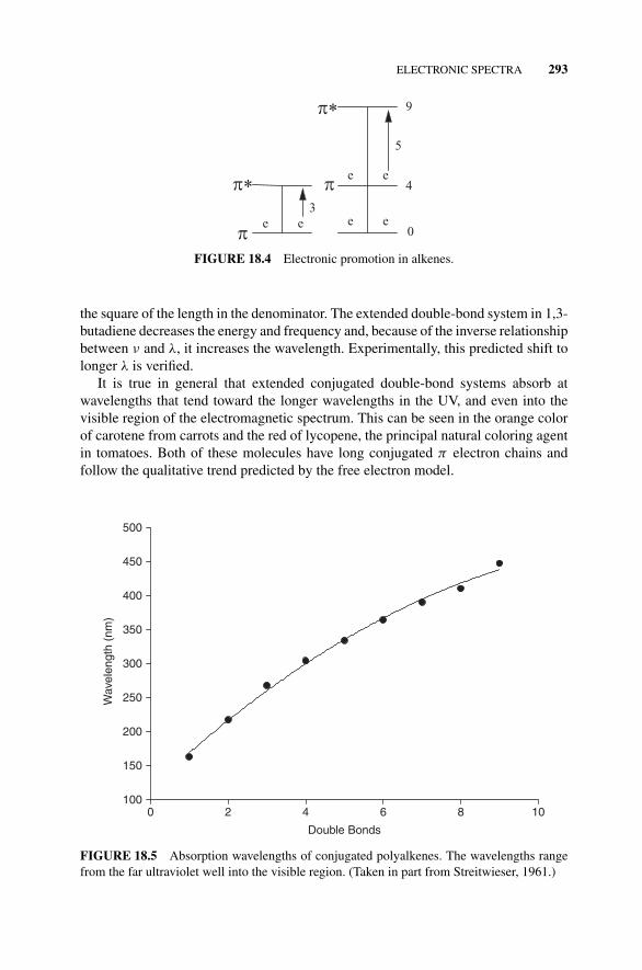
P1: OTA/XYZ P2: ABCc18 JWBS043-Rogers September 13, 2010 11:29 Printer Name: Yet to Come
ELECTRONIC SPECTRA 293
9
4
0e e e e
e e
3
5
FIGURE 18.4 Electronic promotion in alkenes.
the square of the length in the denominator. The extended double-bond system in 1,3-butadiene decreases the energy and frequency and, because of the inverse relationshipbetween ν and λ, it increases the wavelength. Experimentally, this predicted shift tolonger λ is verified.
It is true in general that extended conjugated double-bond systems absorb atwavelengths that tend toward the longer wavelengths in the UV, and even into thevisible region of the electromagnetic spectrum. This can be seen in the orange colorof carotene from carrots and the red of lycopene, the principal natural coloring agentin tomatoes. Both of these molecules have long conjugated π electron chains andfollow the qualitative trend predicted by the free electron model.
Double Bonds
86420 10
Wav
elen
gth
(nm
)
100
150
200
250
300
350
400
450
500
FIGURE 18.5 Absorption wavelengths of conjugated polyalkenes. The wavelengths rangefrom the far ultraviolet well into the visible region. (Taken in part from Streitwieser, 1961.)
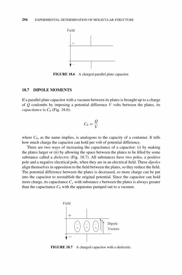
P1: OTA/XYZ P2: ABCc18 JWBS043-Rogers September 13, 2010 11:29 Printer Name: Yet to Come
294 EXPERIMENTAL DETERMINATION OF MOLECULAR STRUCTURE
+
–
Field
FIGURE 18.6 A charged parallel plate capacitor.
18.7 DIPOLE MOMENTS
If a parallel plate capacitor with a vacuum between its plates is brought up to a chargeof Q coulombs by imposing a potential difference V volts between the plates, itscapacitance is C0 (Fig. 18.6):
C0 = Q
V
where C0, as the name implies, is analogous to the capacity of a container. It tellshow much charge the capacitor can hold per volt of potential difference.
There are two ways of increasing the capacitance of a capacitor: (i) by makingthe plates larger or (ii) by allowing the space between the plates to be filled by somesubstance called a dielectric (Fig. 18.7). All substances have two poles, a positivepole and a negative electrical pole, when they are in an electrical field. These dipolesalign themselves in opposition to the field between the plates, so they reduce the field.The potential difference between the plates is decreased, so more charge can be putinto the capacitor to reestablish the original potential. Since the capacitor can holdmore charge, its capacitance Cx with substance x between the plates is always greaterthan the capacitance C0 with the apparatus pumped out to a vacuum.
+
–
Field
–+
–+
–+
Dipole
Vectors
FIGURE 18.7 A charged capacitor with a dielectric.
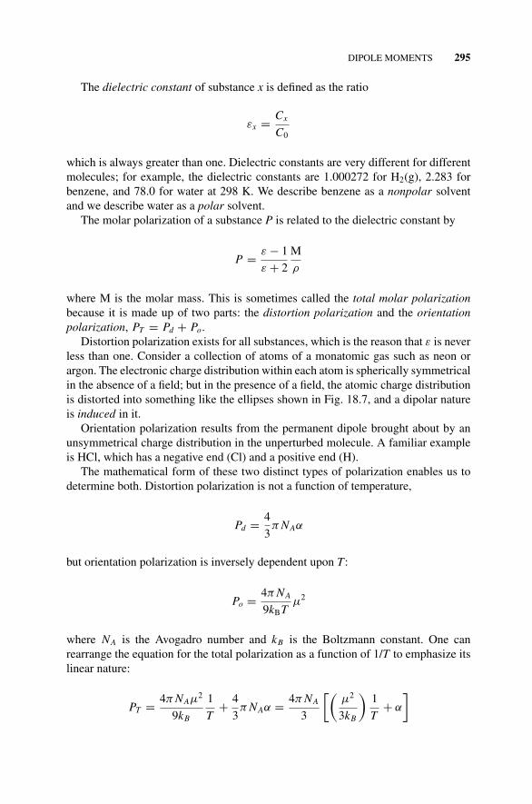
P1: OTA/XYZ P2: ABCc18 JWBS043-Rogers September 13, 2010 11:29 Printer Name: Yet to Come
DIPOLE MOMENTS 295
The dielectric constant of substance x is defined as the ratio
εx = Cx
C0
which is always greater than one. Dielectric constants are very different for differentmolecules; for example, the dielectric constants are 1.000272 for H2(g), 2.283 forbenzene, and 78.0 for water at 298 K. We describe benzene as a nonpolar solventand we describe water as a polar solvent.
The molar polarization of a substance P is related to the dielectric constant by
P = ε − 1
ε + 2
M
ρ
where M is the molar mass. This is sometimes called the total molar polarizationbecause it is made up of two parts: the distortion polarization and the orientationpolarization, PT = Pd + Po.
Distortion polarization exists for all substances, which is the reason that ε is neverless than one. Consider a collection of atoms of a monatomic gas such as neon orargon. The electronic charge distribution within each atom is spherically symmetricalin the absence of a field; but in the presence of a field, the atomic charge distributionis distorted into something like the ellipses shown in Fig. 18.7, and a dipolar natureis induced in it.
Orientation polarization results from the permanent dipole brought about by anunsymmetrical charge distribution in the unperturbed molecule. A familiar exampleis HCl, which has a negative end (Cl) and a positive end (H).
The mathematical form of these two distinct types of polarization enables us todetermine both. Distortion polarization is not a function of temperature,
Pd = 4
3π NAα
but orientation polarization is inversely dependent upon T:
Po = 4π NA
9kBTµ2
where NA is the Avogadro number and kB is the Boltzmann constant. One canrearrange the equation for the total polarization as a function of 1/T to emphasize itslinear nature:
PT = 4π NAµ2
9kB
1
T+ 4
3π NAα = 4π NA
3
[(µ2
3kB
)1
T+ α
]
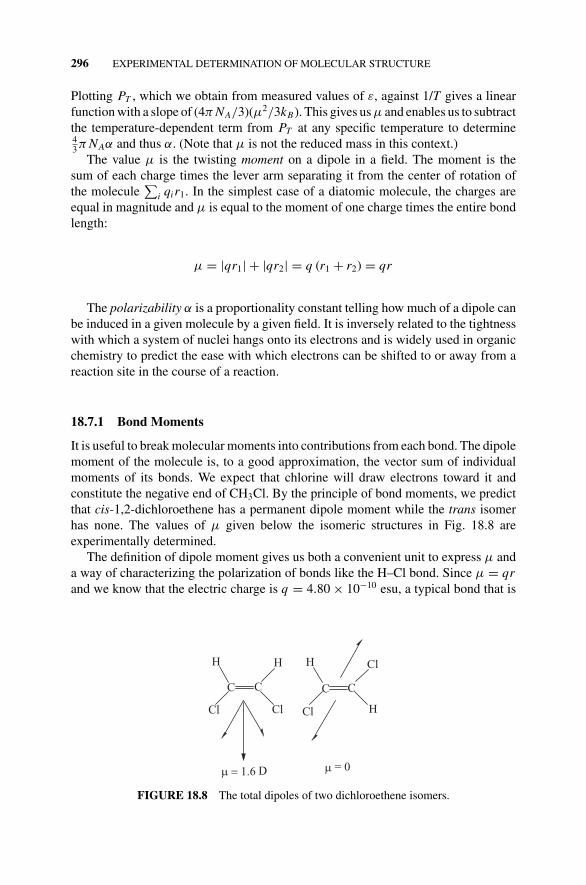
P1: OTA/XYZ P2: ABCc18 JWBS043-Rogers September 13, 2010 11:29 Printer Name: Yet to Come
296 EXPERIMENTAL DETERMINATION OF MOLECULAR STRUCTURE
Plotting PT , which we obtain from measured values of ε, against 1/T gives a linearfunction with a slope of (4π NA/3)(µ2/3kB). This gives us µ and enables us to subtractthe temperature-dependent term from PT at any specific temperature to determine43π NAα and thus α. (Note that µ is not the reduced mass in this context.)
The value µ is the twisting moment on a dipole in a field. The moment is thesum of each charge times the lever arm separating it from the center of rotation ofthe molecule
∑i qir1. In the simplest case of a diatomic molecule, the charges are
equal in magnitude and µ is equal to the moment of one charge times the entire bondlength:
µ = |qr1| + |qr2| = q (r1 + r2) = qr
The polarizability α is a proportionality constant telling how much of a dipole canbe induced in a given molecule by a given field. It is inversely related to the tightnesswith which a system of nuclei hangs onto its electrons and is widely used in organicchemistry to predict the ease with which electrons can be shifted to or away from areaction site in the course of a reaction.
18.7.1 Bond Moments
It is useful to break molecular moments into contributions from each bond. The dipolemoment of the molecule is, to a good approximation, the vector sum of individualmoments of its bonds. We expect that chlorine will draw electrons toward it andconstitute the negative end of CH3Cl. By the principle of bond moments, we predictthat cis-1,2-dichloroethene has a permanent dipole moment while the trans isomerhas none. The values of µ given below the isomeric structures in Fig. 18.8 areexperimentally determined.
The definition of dipole moment gives us both a convenient unit to express µ anda way of characterizing the polarization of bonds like the H–Cl bond. Since µ = qrand we know that the electric charge is q = 4.80 × 10⁻¹⁰ esu, a typical bond that is
C C
H H
Cl Cl
C C
H
Cl
Cl
H
D = 0
FIGURE 18.8 The total dipoles of two dichloroethene isomers.
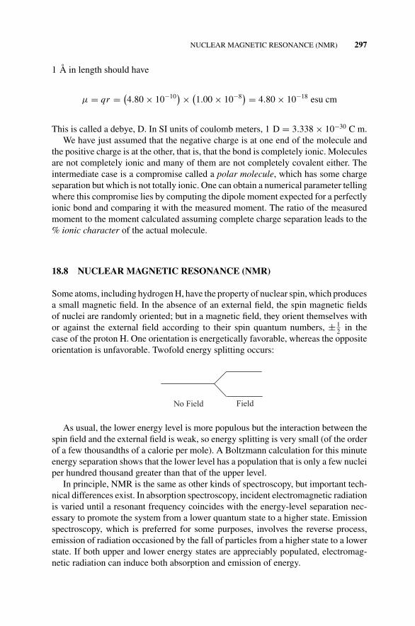
P1: OTA/XYZ P2: ABCc18 JWBS043-Rogers September 13, 2010 11:29 Printer Name: Yet to Come
NUCLEAR MAGNETIC RESONANCE (NMR) 297
1 A in length should have
µ = qr = (4.80 × 10⁻¹⁰) × (
1.00 × 10⁻⁸) = 4.80 × 10⁻¹⁸ esu cm
This is called a debye, D. In SI units of coulomb meters, 1 D = 3.338 × 10⁻³⁰ C m.We have just assumed that the negative charge is at one end of the molecule and
the positive charge is at the other, that is, that the bond is completely ionic. Moleculesare not completely ionic and many of them are not completely covalent either. Theintermediate case is a compromise called a polar molecule, which has some chargeseparation but which is not totally ionic. One can obtain a numerical parameter tellingwhere this compromise lies by computing the dipole moment expected for a perfectlyionic bond and comparing it with the measured moment. The ratio of the measuredmoment to the moment calculated assuming complete charge separation leads to the% ionic character of the actual molecule.
18.8 NUCLEAR MAGNETIC RESONANCE (NMR)
Some atoms, including hydrogen H, have the property of nuclear spin, which producesa small magnetic field. In the absence of an external field, the spin magnetic fieldsof nuclei are randomly oriented; but in a magnetic field, they orient themselves withor against the external field according to their spin quantum numbers, ± 1
2 in thecase of the proton H. One orientation is energetically favorable, whereas the oppositeorientation is unfavorable. Twofold energy splitting occurs:
No Field Field
As usual, the lower energy level is more populous but the interaction between thespin field and the external field is weak, so energy splitting is very small (of the orderof a few thousandths of a calorie per mole). A Boltzmann calculation for this minuteenergy separation shows that the lower level has a population that is only a few nucleiper hundred thousand greater than that of the upper level.
In principle, NMR is the same as other kinds of spectroscopy, but important tech-nical differences exist. In absorption spectroscopy, incident electromagnetic radiationis varied until a resonant frequency coincides with the energy-level separation nec-essary to promote the system from a lower quantum state to a higher state. Emissionspectroscopy, which is preferred for some purposes, involves the reverse process,emission of radiation occasioned by the fall of particles from a higher state to a lowerstate. If both upper and lower energy states are appreciably populated, electromag-netic radiation can induce both absorption and emission of energy.
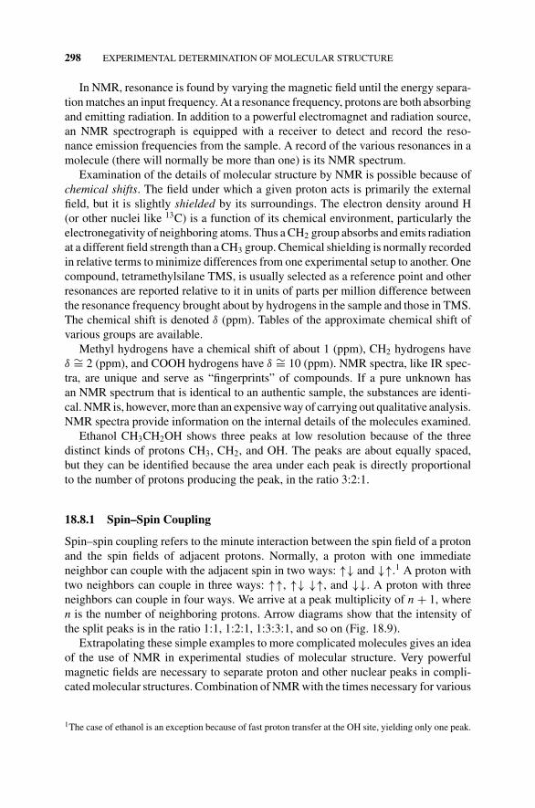
P1: OTA/XYZ P2: ABCc18 JWBS043-Rogers September 13, 2010 11:29 Printer Name: Yet to Come
298 EXPERIMENTAL DETERMINATION OF MOLECULAR STRUCTURE
In NMR, resonance is found by varying the magnetic field until the energy separa-tion matches an input frequency. At a resonance frequency, protons are both absorbingand emitting radiation. In addition to a powerful electromagnet and radiation source,an NMR spectrograph is equipped with a receiver to detect and record the reso-nance emission frequencies from the sample. A record of the various resonances in amolecule (there will normally be more than one) is its NMR spectrum.
Examination of the details of molecular structure by NMR is possible because ofchemical shifts. The field under which a given proton acts is primarily the externalfield, but it is slightly shielded by its surroundings. The electron density around H(or other nuclei like 13C) is a function of its chemical environment, particularly theelectronegativity of neighboring atoms. Thus a CH2 group absorbs and emits radiationat a different field strength than a CH3 group. Chemical shielding is normally recordedin relative terms to minimize differences from one experimental setup to another. Onecompound, tetramethylsilane TMS, is usually selected as a reference point and otherresonances are reported relative to it in units of parts per million difference betweenthe resonance frequency brought about by hydrogens in the sample and those in TMS.The chemical shift is denoted δ (ppm). Tables of the approximate chemical shift ofvarious groups are available.
Methyl hydrogens have a chemical shift of about 1 (ppm), CH2 hydrogens haveδ ∼= 2 (ppm), and COOH hydrogens have δ ∼= 10 (ppm). NMR spectra, like IR spec-tra, are unique and serve as “fingerprints” of compounds. If a pure unknown hasan NMR spectrum that is identical to an authentic sample, the substances are identi-cal. NMR is, however, more than an expensive way of carrying out qualitative analysis.NMR spectra provide information on the internal details of the molecules examined.
Ethanol CH3CH2OH shows three peaks at low resolution because of the threedistinct kinds of protons CH3, CH2, and OH. The peaks are about equally spaced,but they can be identified because the area under each peak is directly proportionalto the number of protons producing the peak, in the ratio 3:2:1.
18.8.1 Spin–Spin Coupling
Spin–spin coupling refers to the minute interaction between the spin field of a protonand the spin fields of adjacent protons. Normally, a proton with one immediateneighbor can couple with the adjacent spin in two ways: ↑↓ and ↓↑.1 A proton withtwo neighbors can couple in three ways: ↑↑, ↑↓ ↓↑, and ↓↓. A proton with threeneighbors can couple in four ways. We arrive at a peak multiplicity of n + 1, wheren is the number of neighboring protons. Arrow diagrams show that the intensity ofthe split peaks is in the ratio 1:1, 1:2:1, 1:3:3:1, and so on (Fig. 18.9).
Extrapolating these simple examples to more complicated molecules gives an ideaof the use of NMR in experimental studies of molecular structure. Very powerfulmagnetic fields are necessary to separate proton and other nuclear peaks in compli-cated molecular structures. Combination of NMR with the times necessary for various
1The case of ethanol is an exception because of fast proton transfer at the OH site, yielding only one peak.
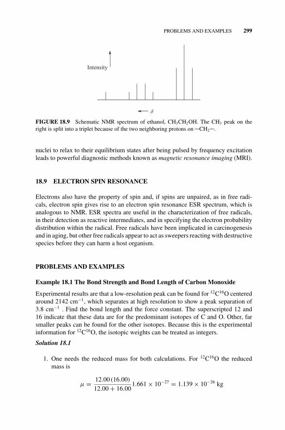
P1: OTA/XYZ P2: ABCc18 JWBS043-Rogers September 13, 2010 11:29 Printer Name: Yet to Come
PROBLEMS AND EXAMPLES 299
Intensity
FIGURE 18.9 Schematic NMR spectrum of ethanol, CH3CH2OH. The CH3 peak on theright is split into a triplet because of the two neighboring protons on CH2 .
nuclei to relax to their equilibrium states after being pulsed by frequency excitationleads to powerful diagnostic methods known as magnetic resonance imaging (MRI).
18.9 ELECTRON SPIN RESONANCE
Electrons also have the property of spin and, if spins are unpaired, as in free radi-cals, electron spin gives rise to an electron spin resonance ESR spectrum, which isanalogous to NMR. ESR spectra are useful in the characterization of free radicals,in their detection as reactive intermediates, and in specifying the electron probabilitydistribution within the radical. Free radicals have been implicated in carcinogenesisand in aging, but other free radicals appear to act as sweepers reacting with destructivespecies before they can harm a host organism.
PROBLEMS AND EXAMPLES
Example 18.1 The Bond Strength and Bond Length of Carbon Monoxide
Experimental results are that a low-resolution peak can be found for 12C16O centeredaround 2142 cm−1, which separates at high resolution to show a peak separation of3.8 cm−1 . Find the bond length and the force constant. The superscripted 12 and16 indicate that these data are for the predominant isotopes of C and O. Other, farsmaller peaks can be found for the other isotopes. Because this is the experimentalinformation for 12C16O, the isotopic weights can be treated as integers.
Solution 18.1
1. One needs the reduced mass for both calculations. For 12C16O the reducedmass is
µ = 12.00 (16.00)
12.00 + 16.001.661 × 10−27 = 1.139 × 10⁻²⁶ kg
P1: OTA/XYZ P2: ABCc18 JWBS043-Rogers September 13, 2010 11:29 Printer Name: Yet to Come
300 EXPERIMENTAL DETERMINATION OF MOLECULAR STRUCTURE
Low Resolution High Resolution
Frequency
FIGURE 18.10 Schematic diagram of a vibration–rotation band. The low-resolution vibra-tional band contains many rotational lines that may be discernable at high resolution. Theseparation between rotational lines is given the term 2B.
2. The force constant is extracted from the classical expression for simple har-monic motion:
ν = 1
2π
√k f
m
Given the experimental measurement of ν = 2142 cm−1 = 2.142 × 10⁵ m−1,the frequency is
ν = cν = (2.998 × 10⁸ m s−1
),
(2.142 × 10⁵ m−1
) = 6.422 × 10¹³ s−1
From the harmonic oscillator approximation
ν = 1
2π
√k f
m
we get
k f
m= 4π2ν2 = 1.628 × 1029
Substituting the reduced mass of 12C16O for m, we obtain
k f = µ × (4π2 ν2
0
) = (1.138 × 10⁻²⁶
) × (1.628 × 1029
) = 1853 N m−1
3. The bond length is found from the moment of inertia of the molecule modeledas a rigid rotor. The energy spacing is
2B = 2h2
2I= h2
4π2 I
P1: OTA/XYZ P2: ABCc18 JWBS043-Rogers September 13, 2010 11:29 Printer Name: Yet to Come
PROBLEMS AND EXAMPLES 301
The spectral input to this calculation is the line separation
2B = 3.8604 cm−1 = 386.04 m−1
so B = 193.02 m−1. This is multiplied by c to obtain the frequency in s−1 andbond length r in pm:
I = h
4π2 (2Bc)= 2.799 × 10−44
B= 2.799 × 10−44
193.02= 1.450 × 10−46
r2 = 1.450 × 10−46
1.138 × 10−26= 1.27 × 10⁻²⁰
r = 1.129 × 10⁻¹⁰ m = 112.9 pm
Example 18.2 The Dipole Moment of Sulfur Dioxide
Sulfur dioxide, SO2, has a total molar polarization of 68.2 cm3 mol−1 at 298 K and56.0 cm3 mol−1 at 398 K. What is the dipole moment of SO2?
Solution 18.2 The inverse of the lower temperature is 0.00336 and the in-verse of the upper temperature is 0.00251. The molar polarizations are 68.2 and56.0 cm3 mol−1. The slope of the curve of molar polarization vs. the inverse ofT is 1.44 × 104 cm3 K mol−1. (Probably for historical reasons, the nonstandard unitsystem of erg cm is often used.) The experimental slope is related to the dipolemoment as
slope = 4π NAµ2
9kB= 1.44 × 10⁴
Solving for µ2, we get
µ2 = 9kB
4π NAslope = 1.641 × 10−47
(1.44 × 10⁴
)
It is convenient at this point to change the units of kB from J K−1 to erg K−1. Thisrequires multiplication by 107 to give
µ2 = 1.641 × 10−40 (1.44 × 10⁴) = 2.363 × 10−36
µ =√
2.363 × 10−36 = 1.54 × 10−18 = 1.54 D
Problem 18.1
The molecule 1H35Cl absorbs light at λ = 2.991 × 10⁻⁴ cm = 2.991 × 10⁻⁶ m. Tak-ing 1H35Cl to be a harmonic oscillator, what are the differences in energy between
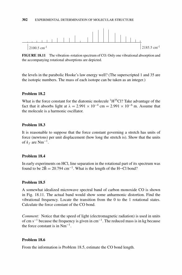
P1: OTA/XYZ P2: ABCc18 JWBS043-Rogers September 13, 2010 11:29 Printer Name: Yet to Come
302 EXPERIMENTAL DETERMINATION OF MOLECULAR STRUCTURE
2100.5 cm-1 2185.5 cm-1
FIGURE 18.11 The vibration–rotation spectrum of CO. Only one vibrational absorption andthe accompanying rotational absorptions are depicted.
the levels in the parabolic Hooke’s law energy well? (The superscripted 1 and 35 arethe isotopic numbers. The mass of each isotope can be taken as an integer.)
Problem 18.2
What is the force constant for the diatomic molecule 1H35Cl? Take advantage of thefact that it absorbs light at λ = 2.991 × 10⁻⁴ cm = 2.991 × 10⁻⁶ m. Assume thatthe molecule is a harmonic oscillator.
Problem 18.3
It is reasonable to suppose that the force constant governing a stretch has units offorce (newtons) per unit displacement (how long the stretch is). Show that the unitsof k f are Nm−1.
Problem 18.4
In early experiments on HCl, line separation in the rotational part of its spectrum wasfound to be 2B = 20.794 cm−1. What is the length of the H Cl bond?
Problem 18.5
A somewhat idealized microwave spectral band of carbon monoxide CO is shownin Fig. 18.11. The actual band would show some anharmonic distortion. Find thevibrational frequency. Locate the transition from the 0 to the 1 rotational states.Calculate the force constant of the CO bond.
Comment: Notice that the speed of light (electromagnetic radiation) is used in unitsof cm s−1 because the frequency is given in cm−1. The reduced mass is in kg becausethe force constant is in Nm−1.
Problem 18.6
From the information is Problem 18.5, estimate the CO bond length.
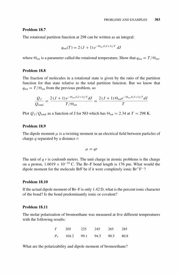
P1: OTA/XYZ P2: ABCc18 JWBS043-Rogers September 13, 2010 11:29 Printer Name: Yet to Come
PROBLEMS AND EXAMPLES 303
Problem 18.7
The rotational partition function at 298 can be written as an integral:
qrot(T ) = 2 (J + 1) e−rot J (J+1)/T dJ
where rot is a parameter called the rotational temperature, Show that qrot = T/rot.
Problem 18.8
The fraction of molecules in a rotational state is given by the ratio of the partitionfunction for that state relative to the total partition function. But we know thatqrot = T/rot from the previous problem, so
Q J
Qtotal= 2 (J + 1) e−rot J (J+1)/T dJ
T/rot= 2 (J + 1) rote−rot J (J+1)/T dJ
T
Plot Q J /Qtotal as a function of J for NO which has rot = 2.34 at T = 298 K.
Problem 18.9
The dipole moment µ is a twisting moment in an electrical field between particles ofcharge q separated by a distance r:
µ = qr
The unit of q r is coulomb meters. The unit charge in atomic problems is the chargeon a proton, 1.6019 × 10⁻¹⁹ C. The Br–F bond length is 176 pm. What would thedipole moment for the molecule BrF be if it were completely ionic Br+F−?
Problem 18.10
If the actual dipole moment of Br–F is only 1.42 D, what is the percent ionic characterof the bond? Is the bond predominantly ionic or covalent?
Problem 18.11
The molar polarization of bromoethane was measured at five different temperatureswith the following results:
T 205 225 245 265 285
PT 104.2 99.1 94.5 90.5 80.8
What are the polarizability and dipole moment of bromoethane?
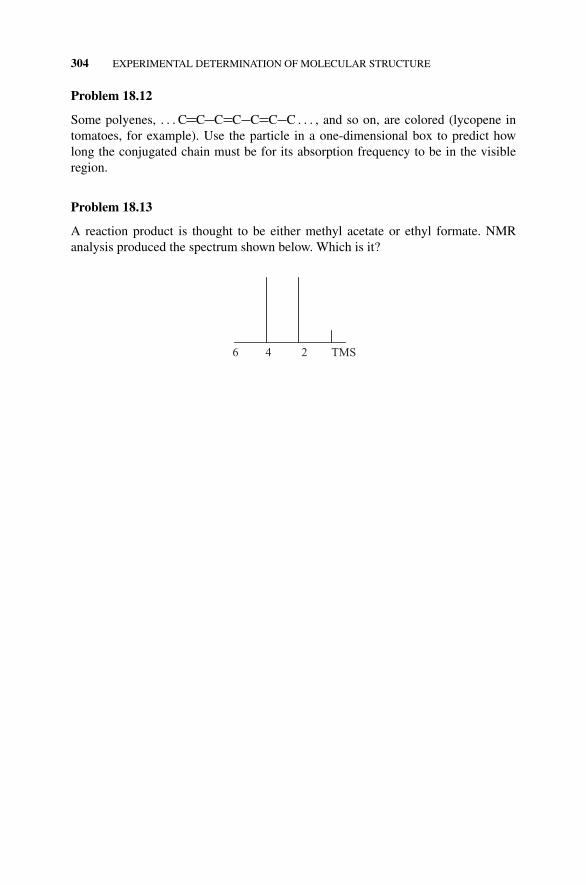
P1: OTA/XYZ P2: ABCc18 JWBS043-Rogers September 13, 2010 11:29 Printer Name: Yet to Come
304 EXPERIMENTAL DETERMINATION OF MOLECULAR STRUCTURE
Problem 18.12
Some polyenes, . . . C C C C C C C . . . , and so on, are colored (lycopene intomatoes, for example). Use the particle in a one-dimensional box to predict howlong the conjugated chain must be for its absorption frequency to be in the visibleregion.
Problem 18.13
A reaction product is thought to be either methyl acetate or ethyl formate. NMRanalysis produced the spectrum shown below. Which is it?
6 4 2 TMS
P1: OTA/XYZ P2: ABCc19 JWBS043-Rogers September 13, 2010 11:29 Printer Name: Yet to Come
19CLASSICAL MOLECULAR MODELING
Although the chemical bond is a result of quantum mechanical interactions of elec-trons with nuclei and with each other, the atom itself is large enough to be treatedclassically. One way of understanding and predicting chemical properties is by treat-ing the molecule as an aggregation of atoms bound by classical bonds and interactingwith each other in a classical way. Such a study is called molecular mechanics, MM.
19.1 ENTHALPY: ADDITIVE METHODS
It has long been known that extension of an alkane chain by one CH2 group
CH3(CH2)nCH3 → CH3(CH2)n+1CH3
brings about a decrease in the � f H 298 of about 5 kcal mol−1 = 21 kJ mol−1
(Fig. 19.1). For example, if we subtract 21 kJ mol−1 from � f H 298(ethane) =−84 kJ mol−1, we get (correctly) � f H 298(propane) = −105 kJ mol−1. Thus we cancall –21 kJ mol−1 a CH2 group enthalpy for the extension of ethane to propane. Thegroup enthalpy is transferable to give the enthalpy change for extension of otheralkanes to an alkane larger by one CH2 group.
If this works for CH2, why not try it with other alkyl groups? The enthalpy ofthe CH3 group must be one-half the enthalpy of formation of the ethane moleculeCH3CH3, � f H 298(ethane) = –84 kJ mol−1. Hence we take the CH3 group enthalpy
Concise Physical Chemistry, by Donald W. RogersCopyright C© 2011 John Wiley & Sons, Inc.
305
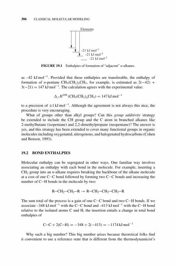
P1: OTA/XYZ P2: ABCc19 JWBS043-Rogers September 13, 2010 11:29 Printer Name: Yet to Come
306 CLASSICAL MOLECULAR MODELING
Elements
-21 kJ mol-1
-21 kJ mol-1
-21 kJ mol-1
FIGURE 19.1 Enthalpies of formation of “adjacent” n-alkanes.
as –42 kJ mol−1. Provided that these enthalpies are transferable, the enthalpy offormation of n-pentane CH3(CH2)3CH3, for example, is estimated as 2(−42) +3(−21) = 147 kJ mol−1. The calculation agrees with the experimental value:
� f H 298 (CH3(CH2)nCH3) = 147 kJ mol−1
to a precision of ±1 kJ mol−1. Although the agreement is not always this nice, theprocedure is very encouraging.
What of groups other than alkyl groups? Can this group additivity strategybe extended to include the CH group and the C atom in branched alkanes like2-methylbutane (isopentane) and 2,2-dimethylpropane (neopentane)? The answer isyes, and this strategy has been extended to cover many functional groups in organicmolecules including oxygenated, nitrogenous, and halogenated hydrocarbons (Cohenand Benson, 1993).
19.2 BOND ENTHALPIES
Molecular enthalpy can be segregated in other ways. One familiar way involvesassociating an enthalpy with each bond in the molecule. For example, inserting aCH2 group into an n-alkane requires breaking the backbone of the alkane moleculeat a cost of one C C bond followed by forming two C C bonds and increasing thenumber of C H bonds in the molecule by two:
R CH2 CH2 R → R CH2 CH2 CH2 R
The sum total of the process is a gain of one C C bond and two C H bonds. If weassociate –348 kJ mol−1 with the C C bond and –413 kJ mol−1 with the C H bondrelative to the isolated atoms C and H, the insertion entails a change in total bondenthalpies of
C C + 2(C H) = −348 + 2(−413) = −1174 kJ mol−1
Why such a big number? This big number arises because theoretical folks findit convenient to use a reference state that is different from the thermodynamicist’s
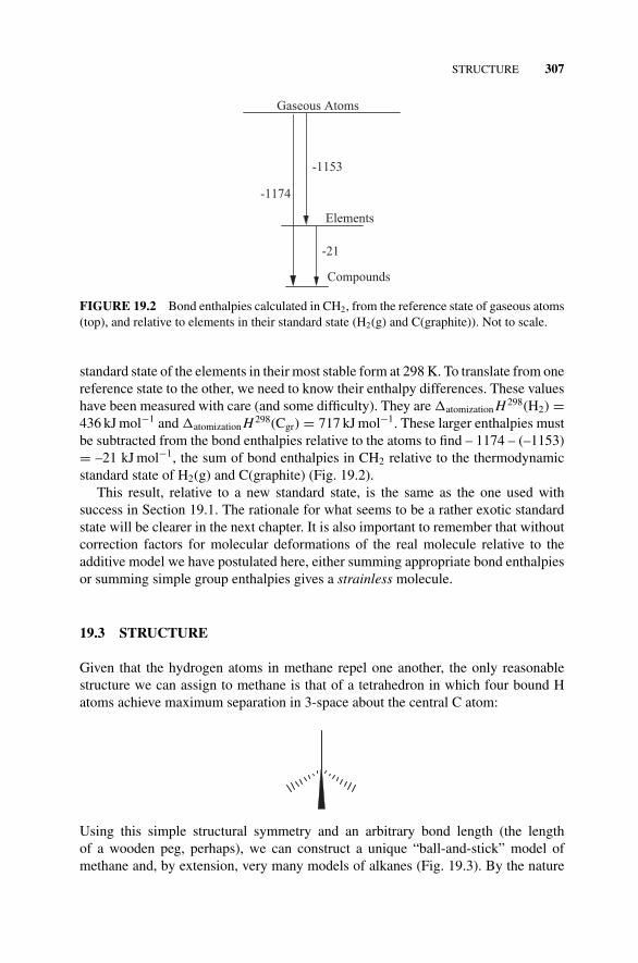
P1: OTA/XYZ P2: ABCc19 JWBS043-Rogers September 13, 2010 11:29 Printer Name: Yet to Come
STRUCTURE 307
Elements
Gaseous Atoms
Compounds
-1153
-1174
-21
FIGURE 19.2 Bond enthalpies calculated in CH2, from the reference state of gaseous atoms(top), and relative to elements in their standard state (H2(g) and C(graphite)). Not to scale.
standard state of the elements in their most stable form at 298 K. To translate from onereference state to the other, we need to know their enthalpy differences. These valueshave been measured with care (and some difficulty). They are �atomization H 298(H2) =436 kJ mol−1 and �atomization H 298(Cgr) = 717 kJ mol−1. These larger enthalpies mustbe subtracted from the bond enthalpies relative to the atoms to find – 1174 – (–1153)= –21 kJ mol−1, the sum of bond enthalpies in CH2 relative to the thermodynamicstandard state of H2(g) and C(graphite) (Fig. 19.2).
This result, relative to a new standard state, is the same as the one used withsuccess in Section 19.1. The rationale for what seems to be a rather exotic standardstate will be clearer in the next chapter. It is also important to remember that withoutcorrection factors for molecular deformations of the real molecule relative to theadditive model we have postulated here, either summing appropriate bond enthalpiesor summing simple group enthalpies gives a strainless molecule.
19.3 STRUCTURE
Given that the hydrogen atoms in methane repel one another, the only reasonablestructure we can assign to methane is that of a tetrahedron in which four bound Hatoms achieve maximum separation in 3-space about the central C atom:
Using this simple structural symmetry and an arbitrary bond length (the lengthof a wooden peg, perhaps), we can construct a unique “ball-and-stick” model ofmethane and, by extension, very many models of alkanes (Fig. 19.3). By the nature
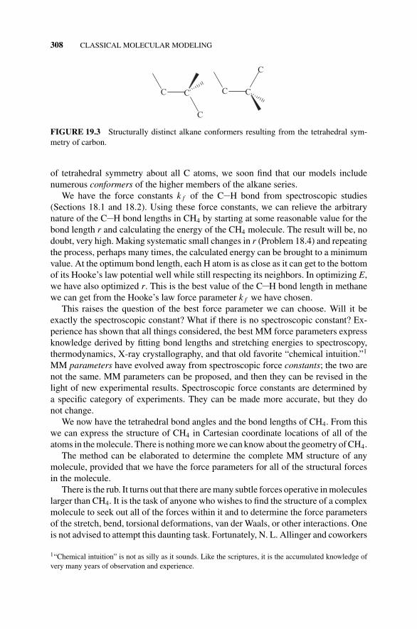
P1: OTA/XYZ P2: ABCc19 JWBS043-Rogers September 13, 2010 11:29 Printer Name: Yet to Come
308 CLASSICAL MOLECULAR MODELING
CC CC
C
C
FIGURE 19.3 Structurally distinct alkane conformers resulting from the tetrahedral sym-metry of carbon.
of tetrahedral symmetry about all C atoms, we soon find that our models includenumerous conformers of the higher members of the alkane series.
We have the force constants k f of the C H bond from spectroscopic studies(Sections 18.1 and 18.2). Using these force constants, we can relieve the arbitrarynature of the C H bond lengths in CH4 by starting at some reasonable value for thebond length r and calculating the energy of the CH4 molecule. The result will be, nodoubt, very high. Making systematic small changes in r (Problem 18.4) and repeatingthe process, perhaps many times, the calculated energy can be brought to a minimumvalue. At the optimum bond length, each H atom is as close as it can get to the bottomof its Hooke’s law potential well while still respecting its neighbors. In optimizing E,we have also optimized r. This is the best value of the C H bond length in methanewe can get from the Hooke’s law force parameter k f we have chosen.
This raises the question of the best force parameter we can choose. Will it beexactly the spectroscopic constant? What if there is no spectroscopic constant? Ex-perience has shown that all things considered, the best MM force parameters expressknowledge derived by fitting bond lengths and stretching energies to spectroscopy,thermodynamics, X-ray crystallography, and that old favorite “chemical intuition.”1
MM parameters have evolved away from spectroscopic force constants; the two arenot the same. MM parameters can be proposed, and then they can be revised in thelight of new experimental results. Spectroscopic force constants are determined bya specific category of experiments. They can be made more accurate, but they donot change.
We now have the tetrahedral bond angles and the bond lengths of CH4. From thiswe can express the structure of CH4 in Cartesian coordinate locations of all of theatoms in the molecule. There is nothing more we can know about the geometry of CH4.
The method can be elaborated to determine the complete MM structure of anymolecule, provided that we have the force parameters for all of the structural forcesin the molecule.
There is the rub. It turns out that there are many subtle forces operative in moleculeslarger than CH4. It is the task of anyone who wishes to find the structure of a complexmolecule to seek out all of the forces within it and to determine the force parametersof the stretch, bend, torsional deformations, van der Waals, or other interactions. Oneis not advised to attempt this daunting task. Fortunately, N. L. Allinger and coworkers
1“Chemical intuition” is not as silly as it sounds. Like the scriptures, it is the accumulated knowledge ofvery many years of observation and experience.
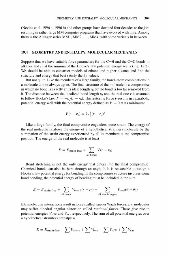
P1: OTA/XYZ P2: ABCc19 JWBS043-Rogers September 13, 2010 11:29 Printer Name: Yet to Come
GEOMETRY AND ENTHALPY: MOLECULAR MECHANICS 309
(Nevins et al. 1996 a, 1996 b) and other groups have devoted four decades to the job,resulting in rather large MM computer programs that have evolved with time. Amongthem is the Allinger series MM1, MM2, . . . , MM4, with some variants in between.
19.4 GEOMETRY AND ENTHALPY: MOLECULAR MECHANICS
Suppose that we have suitable force parameters for the C H and the C C bonds inalkanes and r0 at the minima of the Hooke’s law potential energy wells (Fig. 18.2).We should be able to construct models of ethane and higher alkanes and find thestructure and energy that best satisfy the k f values.
But not quite. Like the members of a large family, the bond–atom combinations ina molecule do not always agree. The final structure of the molecule is a compromisein which no bond is exactly at its ideal length r0 but no bond is too far removed fromit. The distance between the idealized bond length r0 and the real one r is assumedto follow Hooke’s law, F = −k f (r − r0). The restoring force F results in a parabolicpotential energy well with the potential energy defined as V = 0 at its minimum:
V (r − r0) = k f12 (r − r0)2
Like a large family, the final compromise engenders some strain. The energy ofthe real molecule is above the energy of a hypothetical strainless molecule by thesummation of the strain energy experienced by all its members at the compromiseposition. The energy of the real molecule is at least
E = Estrain-free +∑
all bonds
V (r − r0)
Bond stretching is not the only energy that enters into the final compromise.Chemical bonds can also be bent through an angle θ . It is reasonable to assign aHooke’s law potential energy for bending. If the compromise structure involves somebond bending, the potential energy of bending must be included in the sum
E = Estrain-free +∑
all bonds
Vstretch(r − r0) +∑
all simple angles
Vbend(θ − θ0)
Intramolecular interactions result in forces called van der Waals forces, and moleculesmay suffer dihedral angular distortion called torsional forces. These give rise topotential energies VvdW and Vtor, respectively. The sum of all potential energies overa hypothetical strainless enthalpy is
E = Estrain-free +∑
Vstretch +∑
Vbend +∑
VvdW +∑
Vtors
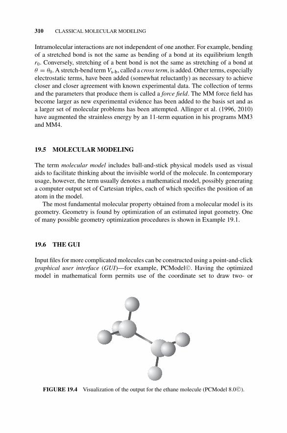
P1: OTA/XYZ P2: ABCc19 JWBS043-Rogers September 13, 2010 11:29 Printer Name: Yet to Come
310 CLASSICAL MOLECULAR MODELING
Intramolecular interactions are not independent of one another. For example, bendingof a stretched bond is not the same as bending of a bond at its equilibrium lengthr0. Conversely, stretching of a bent bond is not the same as stretching of a bond atθ = θ0. A stretch-bend term Vs-b, called a cross term, is added. Other terms, especiallyelectrostatic terms, have been added (somewhat reluctantly) as necessary to achievecloser and closer agreement with known experimental data. The collection of termsand the parameters that produce them is called a force field. The MM force field hasbecome larger as new experimental evidence has been added to the basis set and asa larger set of molecular problems has been attempted. Allinger et al. (1996, 2010)have augmented the strainless energy by an 11-term equation in his programs MM3and MM4.
19.5 MOLECULAR MODELING
The term molecular model includes ball-and-stick physical models used as visualaids to facilitate thinking about the invisible world of the molecule. In contemporaryusage, however, the term usually denotes a mathematical model, possibly generatinga computer output set of Cartesian triples, each of which specifies the position of anatom in the model.
The most fundamental molecular property obtained from a molecular model is itsgeometry. Geometry is found by optimization of an estimated input geometry. Oneof many possible geometry optimization procedures is shown in Example 19.1.
19.6 THE GUI
Input files for more complicated molecules can be constructed using a point-and-clickgraphical user interface (GUI)—for example, PCModel C©. Having the optimizedmodel in mathematical form permits use of the coordinate set to draw two- or
FIGURE 19.4 Visualization of the output for the ethane molecule (PCModel 8.0 C©).
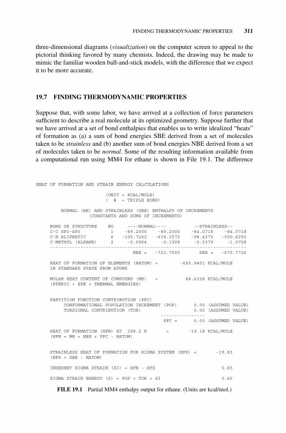
P1: OTA/XYZ P2: ABCc19 JWBS043-Rogers September 13, 2010 11:29 Printer Name: Yet to Come
FINDING THERMODYNAMIC PROPERTIES 311
three-dimensional diagrams (visualization) on the computer screen to appeal to thepictorial thinking favored by many chemists. Indeed, the drawing may be made tomimic the familiar wooden ball-and-stick models, with the difference that we expectit to be more accurate.
19.7 FINDING THERMODYNAMIC PROPERTIES
Suppose that, with some labor, we have arrived at a collection of force parameterssufficient to describe a real molecule at its optimized geometry. Suppose further thatwe have arrived at a set of bond enthalpies that enables us to write idealized “heats”of formation as (a) a sum of bond energies SBE derived from a set of moleculestaken to be strainless and (b) another sum of bond energies NBE derived from a setof molecules taken to be normal. Some of the resulting information available froma computational run using MM4 for ethane is shown in File 19.1. The difference
HEAT OF FORMATION AND STRAIN ENERGY CALCULATIONS
(UNIT = KCAL/MOLE) ( # = TRIPLE BOND)
NORMAL (BE) AND STRAINLESS (SBE) ENTHALPY OF INCREMENTS (CONSTANTS AND SUMS OF INCREMENTS)
BOND OR STRUCTURE NO ----NORMAL---- --STRAINLESS-- C-C SP3-SP3 1 -89.2005 -89.2005 -84.0718 -84.0718 C-H ALIPHATIC 6 -105.7262 -634.3572 -98.4375 -590.6250 C-METHYL (ALKANE) 2 -0.0964 -0.1928 -0.5379 -1.0758 ----------------------------------------------------------------------- NBE = -723.7505 SBE = -675.7726
HEAT OF FORMATION OF ELEMENTS (HATOM) = -655.9401 KCAL/MOLE IN STANDARD STATE FROM ATOMS
MOLAR HEAT CONTENT OF COMPOUND (MH) = 48.6328 KCAL/MOLE (STERIC + ZPE + THERMAL ENERGIES)
PARTITION FUNCTION CONTRIBUTION (PFC) CONFORMATIONAL POPULATION INCREMENT (POP) 0.00 (ASSUMED VALUE) TORSIONAL CONTRIBUTION (TOR) 0.00 (ASSUMED VALUE) ---------------- PFC = 0.00 (ASSUMED VALUE)
HEAT OF FORMATION (HFN) AT 298.2 K = -19.18 KCAL/MOLE (HFN = MH + NBE + PFC - HATOM)
STRAINLESS HEAT OF FORMATION FOR SIGMA SYSTEM (HFS) = -19.83 (HFS = SBE - HATOM)
INHERENT SIGMA STRAIN (SI) = HFN - HFS 0.65
SIGMA STRAIN ENERGY (S) = POP + TOR + SI 0.65
FILE 19.1 Partial MM4 enthalpy output for ethane. (Units are kcal/mol.)
P1: OTA/XYZ P2: ABCc19 JWBS043-Rogers September 13, 2010 11:29 Printer Name: Yet to Come
312 CLASSICAL MOLECULAR MODELING
between SBE and HATOM [the enthalpy input to drive hydrogen and graphite intothe atomic state (Section 19.2) for the strainless molecule] is
� f H 298(strainless) = −675.77 − (−655.94) = −19.83 kcal/mol
A similar sum of normal bond enthalpies gives a different result for the normalmolecule:
NBE + HATOM = � f H 298(normal) + MH = − 67.81 + 48.63 = − 19.18 kcal/mol.
The new term MH (molar heat content) arises from a slightly different way of definingthe normal bond energies; they should be represented by an arrow going all the way tothe bottom of the energy wells in the real molecule. Positive enthalpies—consistingprimarily of the zero point energies of vibration (Section 18.2), with a contributionfrom the steric energy—and small statistical factors add up to a positive correctionof 48.63 kcal/mol. The difference between HFS and HFN is an accumulated strainenergy:
INHERENT SIGMA STRAIN (SI) = HFN - HFS 0.65
The partial MM4 output for ethane (File 19.1) illustrates some other features of theMM procedure and the full file provides more. See STATISTICAL THERMODY-NAMICS ANALYSIS from the MM4 output and Nevins et al. (1996 b, pp. 703–707)for more detail.
19.8 THE OUTSIDE WORLD
In any molecular modeling enterprise, we seek to compare physical properties pre-dicted by the model with the same properties measured by experiment. One obviouschoice is bond lengths as measured by X-ray crystallography. Agreement is usuallygood but not perfect. Even assuming that the impossible task of removing all defectsfrom the model has been achieved, the X-ray crystallographer and the MM modelerare not really looking at the same thing. The idea of a model as developed so farimplies an isolated gas-phase species, but molecules in crystals are subjected to pow-erful forces holding them in the crystalline state due to the sum of forces exerted bytheir neighbors.
Somewhat surprisingly, these forces do not influence bond lengths very much.Agreement between X-ray bond lengths and MM4 lengths is usually within about0.002 A. Simple bond angles, being weaker, are distorted by a few degrees, andtorsional angles, being weaker still, are distorted more. X-rays are scattered byelectrons, so crystallographic structures represent the centers of electron densitieswhich tend to be the same as the location of the nuclei, but which may be displacedin some chemical bonds. For example, the difference between the C H bond length
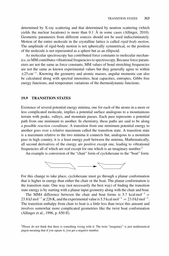
P1: OTA/XYZ P2: ABCc19 JWBS043-Rogers September 13, 2010 11:29 Printer Name: Yet to Come
TRANSITION STATES 313
determined by X-ray scattering and that determined by neutron scattering (whichyields the nuclear locations) is more than 0.1 A in some cases (Allinger, 2010).Geometric parameters from different sources should not be used indiscriminately.Motion of the entire molecule in the crystalline lattice is called rigid-body motion.The amplitude of rigid-body motion is not spherically symmetrical, so the positionof the molecule is not represented as a sphere but as an ellipsoid.
As molecular spectroscopy has contributed force constants to molecular mechan-ics, so MM contributes vibrational frequencies to spectroscopy. Because force param-eters are not the same as force constants, MM values of bond stretching frequenciesare not the same as known experimental values but they generally agree to within±25 cm−1. Knowing the geometry and atomic masses, angular momenta can alsobe calculated along with spectral intensities, heat capacities, entropies, Gibbs freeenergy functions, and temperature variations of the thermodynamic functions.
19.9 TRANSITION STATES
Existence of several potential energy minima, one for each of the atoms in a more orless complicated molecule, implies a potential surface analogous to a mountainousterrain with peaks, valleys, and mountain passes. Each pass represents a potentialpath from one minimum to another. In chemistry, these paths are said to be alonga possible reaction coordinate. A transition from one minimum potential energy toanother goes over a relative maximum called the transition state. A transition stateis a maximum relative to the two minima it connects but, analogous to a mountainpass in high country, it is a least energy path between the minima, Mathematically,all second derivatives of the energy are positive except one, leading to vibrationalfrequencies all of which are real except for one which is an imaginary number.2
An example is conversion of the “chair” form of cyclohexane to the “boat” form:
For this change to take place, cyclohexane must go through a planar conformationthat is higher in energy than either the chair or the boat. The planar conformation isthe transition state. One way (not necessarily the best way) of finding the transitionstate energy is by starting with a planar input geometry along with the chair and boat.
The MM4 difference between the chair and boat forms is 5.7 kcal mol−1 =23.8 kJ mol−1 at 226 K, and the experimental value is 5.5 kcal mol−1 = 23.0 kJ mol−1.The transition enthalpy from chair to boat is a little less than twice this amount andinvolves somewhat more complicated geometries like the twist boat conformation(Allinger et al., 1996, p. 650 ff).
2Please do not think that there is something wrong with it: The term “imaginary” is just mathematicaljargon meaning that if you square it, you get a negative number.
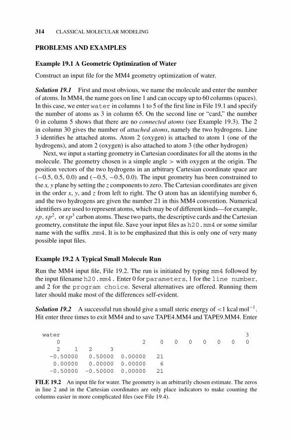
P1: OTA/XYZ P2: ABCc19 JWBS043-Rogers September 13, 2010 11:29 Printer Name: Yet to Come
314 CLASSICAL MOLECULAR MODELING
PROBLEMS AND EXAMPLES
Example 19.1 A Geometric Optimization of Water
Construct an input file for the MM4 geometry optimization of water.
Solution 19.1 First and most obvious, we name the molecule and enter the numberof atoms. In MM4, the name goes on line 1 and can occupy up to 60 columns (spaces).In this case, we enter water in columns 1 to 5 of the first line in File 19.1 and specifythe number of atoms as 3 in column 65. On the second line or “card,” the number0 in column 5 shows that there are no connected atoms (see Example 19.3). The 2in column 30 gives the number of attached atoms, namely the two hydrogens. Line3 identifies he attached atoms. Atom 2 (oxygen) is attached to atom 1 (one of thehydrogens), and atom 2 (oxygen) is also attached to atom 3 (the other hydrogen)
Next, we input a starting geometry in Cartesian coordinates for all the atoms in themolecule. The geometry chosen is a simple angle > with oxygen at the origin. Theposition vectors of the two hydrogens in an arbitrary Cartesian coordinate space are(−0.5, 0.5, 0.0) and (−0.5, −0.5, 0.0). The input geometry has been constrained tothe x, y plane by setting the z components to zero. The Cartesian coordinates are givenin the order x, y, and z from left to right. The O atom has an identifying number 6,and the two hydrogens are given the number 21 in this MM4 convention. Numericalidentifiers are used to represent atoms, which may be of different kinds—for example,sp, sp2, or sp3 carbon atoms. These two parts, the descriptive cards and the Cartesiangeometry, constitute the input file. Save your input files as h20.mm4 or some similarname with the suffix .mm4. It is to be emphasized that this is only one of very manypossible input files.
Example 19.2 A Typical Small Molecule Run
Run the MM4 input file, File 19.2. The run is initiated by typing mm4 followed bythe input filename h20.mm4. Enter 0 for parameters, 1 for the line number,and 2 for the program choice. Several alternatives are offered. Running themlater should make most of the differences self-evident.
Solution 19.2 A successful run should give a small steric energy of <1 kcal mol−1.Hit enter three times to exit MM4 and to save TAPE4.MM4 and TAPE9.MM4. Enter
water 30 2 0 0 0 0 0 0 02 1 2 3
-0.50000 0.50000 0.00000 210.00000 0.00000 0.00000 6
-0.50000 -0.50000 0.00000 21
FILE 19.2 An input file for water. The geometry is an arbitrarily chosen estimate. The zerosin line 2 and in the Cartesian coordinates are only place indicators to make counting thecolumns easier in more complicated files (see File 19.4).
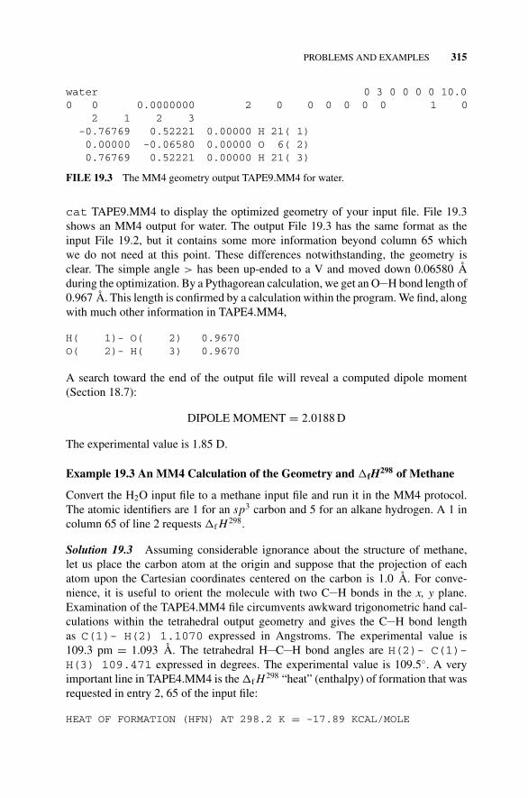
P1: OTA/XYZ P2: ABCc19 JWBS043-Rogers September 13, 2010 11:29 Printer Name: Yet to Come
PROBLEMS AND EXAMPLES 315
water 0 3 0 0 0 0 10.00 0 0.0000000 2 0 0 0 0 0 0 1 0
2 1 2 3-0.76769 0.52221 0.00000 H 21( 1)0.00000 -0.06580 0.00000 O 6( 2)0.76769 0.52221 0.00000 H 21( 3)
FILE 19.3 The MM4 geometry output TAPE9.MM4 for water.
cat TAPE9.MM4 to display the optimized geometry of your input file. File 19.3shows an MM4 output for water. The output File 19.3 has the same format as theinput File 19.2, but it contains some more information beyond column 65 whichwe do not need at this point. These differences notwithstanding, the geometry isclear. The simple angle > has been up-ended to a V and moved down 0.06580 Aduring the optimization. By a Pythagorean calculation, we get an O H bond length of0.967 A. This length is confirmed by a calculation within the program. We find, alongwith much other information in TAPE4.MM4,
H( 1)- O( 2) 0.9670O( 2)- H( 3) 0.9670
A search toward the end of the output file will reveal a computed dipole moment(Section 18.7):
DIPOLE MOMENT = 2.0188 D
The experimental value is 1.85 D.
Example 19.3 An MM4 Calculation of the Geometry and �fH298 of Methane
Convert the H2O input file to a methane input file and run it in the MM4 protocol.The atomic identifiers are 1 for an sp3 carbon and 5 for an alkane hydrogen. A 1 incolumn 65 of line 2 requests �f H 298.
Solution 19.3 Assuming considerable ignorance about the structure of methane,let us place the carbon atom at the origin and suppose that the projection of eachatom upon the Cartesian coordinates centered on the carbon is 1.0 A. For conve-nience, it is useful to orient the molecule with two C H bonds in the x, y plane.Examination of the TAPE4.MM4 file circumvents awkward trigonometric hand cal-culations within the tetrahedral output geometry and gives the C H bond lengthas C(1)- H(2) 1.1070 expressed in Angstroms. The experimental value is109.3 pm = 1.093 A. The tetrahedral H C H bond angles are H(2)- C(1)-H(3) 109.471 expressed in degrees. The experimental value is 109.5◦. A veryimportant line in TAPE4.MM4 is the �f H 298 “heat” (enthalpy) of formation that wasrequested in entry 2, 65 of the input file:
HEAT OF FORMATION (HFN) AT 298.2 K = -17.89 KCAL/MOLE
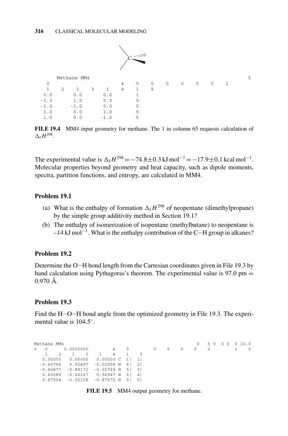
P1: OTA/XYZ P2: ABCc19 JWBS043-Rogers September 13, 2010 11:29 Printer Name: Yet to Come
316 CLASSICAL MOLECULAR MODELING
C
Methane MM4 5 0 4 0 0 0 0 0 0 1 1 2 1 3 1 4 1 5 0.0 0.0 0.0 1 -1.0 1.0 0.0 5 -1.0 -1.0 0.0 5 1.0 0.0 1.0 5 1.0 0.0 -1.0 5
FILE 19.4 MM4 input geometry for methane. The 1 in column 65 requests calculation of�f H 298.
The experimental value is �f H 298 =−74.8±0.3 kJ mol−1 =−17.9±0.1 kcal mol−1.Molecular properties beyond geometry and heat capacity, such as dipole moments,spectra, partition functions, and entropy, are calculated in MM4.
Problem 19.1
(a) What is the enthalpy of formation �f H 298 of neopentane (dimethylpropane)by the simple group additivity method in Section 19.1?
(b) The enthalpy of isomerization of isopentane (methylbutane) to neopentane is–14 kJ mol−1. What is the enthalpy contribution of the C H group in alkanes?
Problem 19.2
Determine the O H bond length from the Cartesian coordinates given in File 19.3 byhand calculation using Pythagoras’s theorem. The experimental value is 97.0 pm =0.970 A.
Problem 19.3
Find the H O H bond angle from the optimized geometry in File 19.3. The experi-mental value is 104.5◦.
Methane MM4 0 5 0 0 0 0 10.0 0 0 0.0000000 4 0 0 0 0 0 1 1 0 1 2 1 3 1 4 1 5 0.00000 0.00000 0.00000 C 1( 1) -0.60766 0.92497 -0.02506 H 5( 2) -0.66877 -0.88172 -0.02769 H 5( 3) 0.60089 -0.02167 0.92947 H 5( 4) 0.67554 -0.02158 -0.87672 H 5( 5)
FILE 19.5 MM4 output geometry for methane.
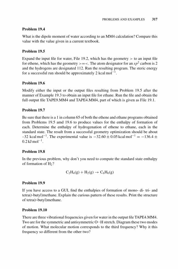
P1: OTA/XYZ P2: ABCc19 JWBS043-Rogers September 13, 2010 11:29 Printer Name: Yet to Come
PROBLEMS AND EXAMPLES 317
Problem 19.4
What is the dipole moment of water according to an MM4 calculation? Compare thisvalue with the value given in a current textbook.
Problem 19.5
Expand the input file for water, File 19.2, which has the geometry > to an input filefor ethene, which has the geometry >=<. The atom designator for an sp2 carbon is 2and the hydrogens are designated 112. Run the resulting program. The steric energyfor a successful run should be approximately 2 kcal mol−1.
Problem 19.6
Modify either the input or the output files resulting from Problem 19.5 after themanner of Example 19.3 to obtain an input file for ethane. Run the file and obtain thefull output file TAPE9.MM4 and TAPE4.MM4, part of which is given as File 19.1.
Problem 19.7
Be sure that there is a 1 in column 65 of both the ethene and ethane programs obtainedfrom Problems 19.5 amd 19.6 to produce values for the enthalpy of formation ofeach. Determine the enthalpy of hydrogenation of ethene to ethane, each in thestandard state. The result from a successful geometry optimization should be about–32 kcal mol−1. The experimental value is −32.60 ± 0.05 kcal mol−1 = −136.4 ±0.2 kJ mol−1.
Problem 19.8
In the previous problem, why don’t you need to compute the standard state enthalpyof formation of H2?
C2H4(g) + H2(g) → C6H6(g)
Problem 19.9
If you have access to a GUI, find the enthalpies of formation of mono- di- tri- andtetra(t-butyl)methane. Explain the curious pattern of these results. Print the structureof tetra(t-butyl)methane.
Problem 19.10
There are three vibrational frequencies given for water in the output file TAPE4.MM4.Two are for the symmetric and antisymmetric O H stretch. Diagram these two modesof motion. What molecular motion corresponds to the third frequency? Why it thisfrequency so different from the other two?
P1: OTA/XYZ P2: ABCc20 JWBS043-Rogers September 13, 2010 11:29 Printer Name: Yet to Come
20QUANTUM MOLECULAR MODELING
With Slater determinants and the Hartree–Fock equations, one had everything neces-sary to solve problems in molecular structure, energy, and dynamics. But the equa-tions could not be solved. Quantum chemistry awaited two spectacular advances.First, Roothaan derived a way to express its apparently insoluble integrodifferentialequations as equations in linear algebra. This was accompanied by an exponentialrise in power of the digital computer, which now routinely carries out trillions ofsimple mathematical operations per second.
The total energy of a molecule is almost entirely that of its constituent atoms,leaving only a fringe energy, which might otherwise be considered trivial, to holdthe molecule together. But it is the chemical bond that dominates the world we seearound us with all its color, life, and diversity, and so it is the chemical bond thatwe seek to calculate. We will be able to extend the atomic orbital concept to ourmolecular calculations but, because chemical energies and energy differences are sosmall, we must achieve a very high level of accuracy. Accurate programs now existthat can be extended to all molecules (in principle at least). Finite computer speedand memory place strict limitations on these grandiose plans, but barriers fall almostevery day in this active research field.
20.1 THE MOLECULAR VARIATIONAL METHOD
The variational method applies to molecules as well as to atoms. By it, we canapproach an optimized molecular energy E:
E = 〈�| H |�〉〈� | �〉
Concise Physical Chemistry, by Donald W. RogersCopyright C© 2011 John Wiley & Sons, Inc.
318
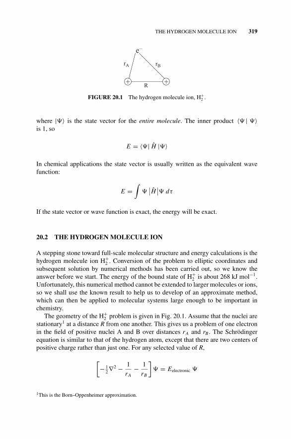
P1: OTA/XYZ P2: ABCc20 JWBS043-Rogers September 13, 2010 11:29 Printer Name: Yet to Come
THE HYDROGEN MOLECULE ION 319
e–
++
rB
R
rA
FIGURE 20.1 The hydrogen molecule ion, H+2 .
where |�〉 is the state vector for the entire molecule. The inner product 〈� | �〉is 1, so
E = 〈�| H |�〉
In chemical applications the state vector is usually written as the equivalent wavefunction:
E =∫
�∣∣H
∣∣� dτ
If the state vector or wave function is exact, the energy will be exact.
20.2 THE HYDROGEN MOLECULE ION
A stepping stone toward full-scale molecular structure and energy calculations is thehydrogen molecule ion H+
2 . Conversion of the problem to elliptic coordinates andsubsequent solution by numerical methods has been carried out, so we know theanswer before we start. The energy of the bound state of H+
2 is about 268 kJ mol−1.Unfortunately, this numerical method cannot be extended to larger molecules or ions,so we shall use the known result to help us to develop of an approximate method,which can then be applied to molecular systems large enough to be important inchemistry.
The geometry of the H+2 problem is given in Fig. 20.1. Assume that the nuclei are
stationary1 at a distance R from one another. This gives us a problem of one electronin the field of positive nuclei A and B over distances rA and rB . The Schrodingerequation is similar to that of the hydrogen atom, except that there are two centers ofpositive charge rather than just one. For any selected value of R,
[− 1
2∇2 − 1
rA− 1
rB
]� = Eelectronic �
1This is the Born–Oppenheimer approximation.
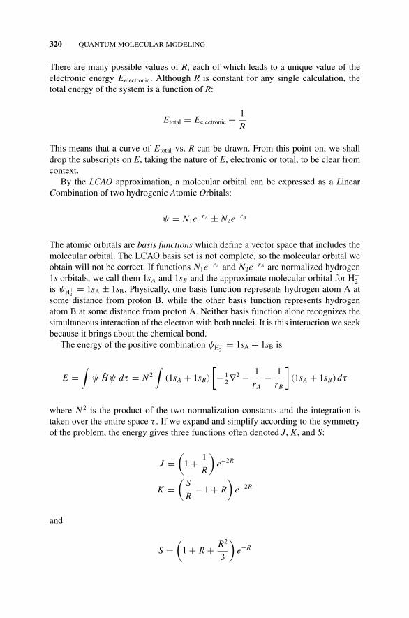
P1: OTA/XYZ P2: ABCc20 JWBS043-Rogers September 13, 2010 11:29 Printer Name: Yet to Come
320 QUANTUM MOLECULAR MODELING
There are many possible values of R, each of which leads to a unique value of theelectronic energy Eelectronic. Although R is constant for any single calculation, thetotal energy of the system is a function of R:
Etotal = Eelectronic + 1
R
This means that a curve of Etotal vs. R can be drawn. From this point on, we shalldrop the subscripts on E, taking the nature of E, electronic or total, to be clear fromcontext.
By the LCAO approximation, a molecular orbital can be expressed as a LinearCombination of two hydrogenic Atomic Orbitals:
ψ = N1e−rA ± N2e−rB
The atomic orbitals are basis functions which define a vector space that includes themolecular orbital. The LCAO basis set is not complete, so the molecular orbital weobtain will not be correct. If functions N1e−rA and N2e−rB are normalized hydrogen1s orbitals, we call them 1sA and 1sB and the approximate molecular orbital for H+
2is ψH+
2= 1sA ± 1sB. Physically, one basis function represents hydrogen atom A at
some distance from proton B, while the other basis function represents hydrogenatom B at some distance from proton A. Neither basis function alone recognizes thesimultaneous interaction of the electron with both nuclei. It is this interaction we seekbecause it brings about the chemical bond.
The energy of the positive combination ψH+2
= 1sA + 1sB is
E =∫
ψ Hψ dτ = N 2∫
(1sA + 1sB)
[− 1
2∇2 − 1
rA− 1
rB
](1sA + 1sB) dτ
where N 2 is the product of the two normalization constants and the integration istaken over the entire space τ . If we expand and simplify according to the symmetryof the problem, the energy gives three functions often denoted J, K, and S:
J =(
1 + 1
R
)e−2R
K =(
S
R− 1 + R
)e−2R
and
S =(
1 + R + R2
3
)e−R
P1: OTA/XYZ P2: ABCc20 JWBS043-Rogers September 13, 2010 11:29 Printer Name: Yet to Come
THE HYDROGEN MOLECULE ION 321
50
0
0.2
EB(R)
EA(R)
R
FIGURE 20.2 Bonding and antibonding orbitals for H+2 . The units of E are hartrees and the
units of R are bohr = 52.9 pm.
which are combined to give
E = J + K
1 + S
The functions J, K, and S are all dependent upon the internuclear separation R becauseorbital interaction is greater when the nuclei are close together and smaller when theyare far apart. The function E = f (R) for the positive combination of atomic orbitalsis shown by the solid curve in Fig. 20.2.
Positive nuclei attracted to an electron between them are bound to each other. Thenuclei do not crash into each other because at some R, internuclear repulsion becomesdominant over bonding and the energy begins to rise sharply. The compromise be-tween attractive and repulsive forces results in a minimum in E = f (R). The bondhas a definite and fixed length of 2.5 bohr = 132 pm in this first approximation. Tofind the energy of the H+
2 bond at this distance, we must solve equations for S, J, andK to give
S = 0.461, J = 0.00963, K = −0.1044, E = −0.065 Eh
The hartree of energy is 1 Eh = 2625 kJ mol−1. The minimum is at E =−0.065 Eh = −171 kJ mol−1. This is about 64% of the experimental value. Thequantitative result is not very good, but the qualitative result shows that the energy isnegative at 132 pm, which indicates bonding. It is noteworthy that the chemical bondarises as a natural consequence of quantum mechanics without further assumptions.
There is a second solution for E in Fig. 20.2 which arises from the negativecombination ψH+
2= 1sA − 1sB. The energy does not go through a minimum with
this antibonding wave function but rises monotonically with decreasing R. In H+2 ,
bonding and antibonding orbitals are above and below the energy of the separatedsystem H+ and H. The higher and lower bonding and antibonding molecular orbitalsat the hond distance are often shown simply as Fig. 20.3.
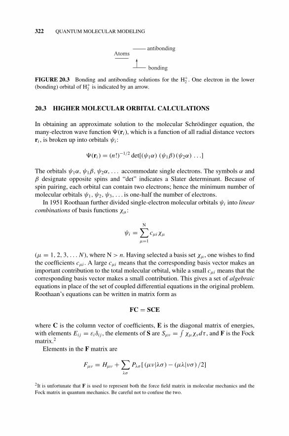
P1: OTA/XYZ P2: ABCc20 JWBS043-Rogers September 13, 2010 11:29 Printer Name: Yet to Come
322 QUANTUM MOLECULAR MODELING
Atomsantibonding
bonding
FIGURE 20.3 Bonding and antibonding solutions for the H+2 . One electron in the lower
(bonding) orbital of H+2 is indicated by an arrow.
20.3 HIGHER MOLECULAR ORBITAL CALCULATIONS
In obtaining an approximate solution to the molecular Schrodinger equation, themany-electron wave function �(ri ), which is a function of all radial distance vectorsri , is broken up into orbitals ψi :
�(ri ) = (n!)−1/2 det[(ψ1α) (ψ1β) (ψ2α) . . .]
The orbitals ψ1α,ψ1β,ψ2α, . . . accommodate single electrons. The symbols α andβ designate opposite spins and “det” indicates a Slater determinant. Because ofspin pairing, each orbital can contain two electrons; hence the minimum number ofmolecular orbitals ψ1, ψ2, ψ3, . . . is one-half the number of electrons.
In 1951 Roothaan further divided single-electron molecular orbitals ψi into linearcombinations of basis functions χµ:
ψi =N∑
µ=1
cµiχµ
(µ = 1, 2, 3, . . . N ), where N > n. Having selected a basis set χµ, one wishes to findthe coefficients cµi . A large cµi means that the corresponding basis vector makes animportant contribution to the total molecular orbital, while a small cµi means that thecorresponding basis vector makes a small contribution. This gives a set of algebraicequations in place of the set of coupled differential equations in the original problem.Roothaan’s equations can be written in matrix form as
FC = SCE
where C is the column vector of coefficients, E is the diagonal matrix of energies,with elements Ei j = εiδi j , the elements of S are Sµν = ∫
χµχνdτ , and F is the Fockmatrix.2
Elements in the F matrix are
Fµν = Hµν +∑λσ
Pλσ [ (µν|λσ ) − (µλ|νσ ) /2]
2It is unfortunate that F is used to represent both the force field matrix in molecular mechanics and theFock matrix in quantum mechanics. Be careful not to confuse the two.
P1: OTA/XYZ P2: ABCc20 JWBS043-Rogers September 13, 2010 11:29 Printer Name: Yet to Come
SEMIEMPIRICAL METHODS 323
defined by
Hµν =∫
χµ Hχνdτ, Pµν = 2n∑1
cµi cνi
and
(µν|λσ ) =∫ ∫
χµ(1)χν(1) × 1
r12χλ (2)χσ (2) dτ1dτ2
(µλ|νσ ) =∫ ∫
χµ(1)χλ(1) × 1
r12χν (2)χσ (2) dτ1dτ2
The matrix elements Hµν are elements of the core Hamiltonian that would be imposedby the nuclei on each electron in the absence of all other electrons, and elements εi
of the diagonal matrix E are one-electron energies. Many computer routines exist formultiplication, inversion, and diagonalization of matrices.
The integrals (µν|λσ ) and (µλ|νσ ) are difficult to evaluate, which caused a bifur-cation of the field of molecular orbital studies into subdisciplines called semiempiricaland ab initio. Research groups led by Dewar and by Stewart were devoted to obtainingsolutions by substituting empirical constants into Fµν . A second approach was fol-lowed by groups led by Pople, Gordon, and others, who used very efficient computercodes and relied upon the increasing power of contemporary computing machines tosolve the integrals in Fµν . In general, the rule of speed vs. accuracy applies. Semiem-pirical substitution is faster, hence applicable to larger molecules. Ab initio methodsare more accurate but they are very expensive in computer resources.
20.4 SEMIEMPIRICAL METHODS
Solution of the Schrodinger equation requires evaluation of many integrals. A largeproportion of these integrals make a very small contribution to molecular energy andenthalpy. When they are dropped, the calculation is simplified in the hope that thesacrifice in accuracy will be small. Dropping the integrals in the equation set leavesonly Hµν in place of the Fock matrix elements Fµν . Dropping some integrals andreplacing others with empirical parameters gives legitimate Hamiltonian elementsbut elements that are approximate because of the use of empirical parameters. Theyare elements Hµν of a semiempirical Hamiltonian operator. The general rule is that ifyou are modifying the F matrix to obtain an approximate Hamiltonian, the method issemiempirical. If you are working with the full F matrix and attempting to approacha complete basis set, the method is ab initio. Neither method is exact.
The most important steps in development of a computer-based semiempiricalmethod were in deciding which of the many integrals (µν|λσ ) and (µλ|νσ ) in apolyatomic molecule can be dropped, which of the integrals must be retained andparameterized, and how they should be parameterized. Neglect of differential overlap
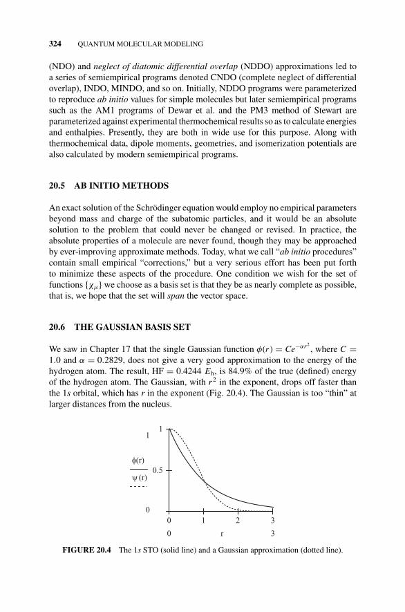
P1: OTA/XYZ P2: ABCc20 JWBS043-Rogers September 13, 2010 11:29 Printer Name: Yet to Come
324 QUANTUM MOLECULAR MODELING
(NDO) and neglect of diatomic differential overlap (NDDO) approximations led toa series of semiempirical programs denoted CNDO (complete neglect of differentialoverlap), INDO, MINDO, and so on. Initially, NDDO programs were parameterizedto reproduce ab initio values for simple molecules but later semiempirical programssuch as the AM1 programs of Dewar et al. and the PM3 method of Stewart areparameterized against experimental thermochemical results so as to calculate energiesand enthalpies. Presently, they are both in wide use for this purpose. Along withthermochemical data, dipole moments, geometries, and isomerization potentials arealso calculated by modern semiempirical programs.
20.5 AB INITIO METHODS
An exact solution of the Schrodinger equation would employ no empirical parametersbeyond mass and charge of the subatomic particles, and it would be an absolutesolution to the problem that could never be changed or revised. In practice, theabsolute properties of a molecule are never found, though they may be approachedby ever-improving approximate methods. Today, what we call “ab initio procedures”contain small empirical “corrections,” but a very serious effort has been put forthto minimize these aspects of the procedure. One condition we wish for the set offunctions {χµ} we choose as a basis set is that they be as nearly complete as possible,that is, we hope that the set will span the vector space.
20.6 THE GAUSSIAN BASIS SET
We saw in Chapter 17 that the single Gaussian function φ(r ) = Ce−αr2, where C =
1.0 and α = 0.2829, does not give a very good approximation to the energy of thehydrogen atom. The result, HF = 0.4244 Eh, is 84.9% of the true (defined) energyof the hydrogen atom. The Gaussian, with r2 in the exponent, drops off faster thanthe 1s orbital, which has r in the exponent (Fig. 20.4). The Gaussian is too “thin” atlarger distances from the nucleus.
10 32
0.5
11
0
(r)
(r)
3r0
FIGURE 20.4 The 1s STO (solid line) and a Gaussian approximation (dotted line).
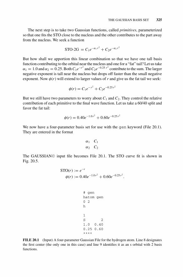
P1: OTA/XYZ P2: ABCc20 JWBS043-Rogers September 13, 2010 11:29 Printer Name: Yet to Come
THE GAUSSIAN BASIS SET 325
The next step is to take two Gaussian functions, called primitives, parameterizedso that one fits the STO close to the nucleus and the other contributes to the part awayfrom the nucleus. We seek a function
STO-2G = C1e−α1 r2 + C2e−α2 r2
But how shall we apportion this linear combination so that we have one tall basisfunction contributing to the orbital near the nucleus and one for a “fat” tail? Let us takeα1 = 1.0 and α2 = 0.25. Both C1e−r2
and C2e−0.25 r2contribute to the sum. The larger
negative exponent is tall near the nucleus but drops off faster than the small negativeexponent. Now φ(r ) will extend to larger values of r and give us the fat tail we seek:
φ(r ) = C1e− r2 + C2e−0.25 r2
But we still have two parameters to worry about C1 and C2. They control the relativecontribution of each primitive to the final wave function. Let us take a 60/40 split andfavor the fat tail:
φ(r ) = 0.40e−1.0 r2 + 0.60e−0.25 r2
We now have a four-parameter basis set for use with the gen keyword (File 20.1).They are entered in the format
α1 C1
α2 C2
The GAUSSIAN C© input file becomes File 20.1. The STO curve fit is shown inFig. 20.5.
STO(r ) := e−r
φ(r ) := 0.40e−1.0 r2 + 0.60e−0.25 r2.
# genhatom gen0 2h
1S 21.0 0.400.25 0.60****
FILE 20.1 (Input) A four-parameter Gaussian File for the hydrogen atom. Line 8 designatesthe first center (the only one in this case) and line 9 identifies it as an s orbital with 2 basisfunctions.
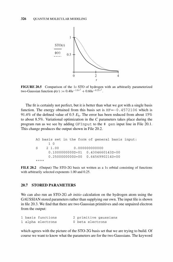
P1: OTA/XYZ P2: ABCc20 JWBS043-Rogers September 13, 2010 11:29 Printer Name: Yet to Come
326 QUANTUM MOLECULAR MODELING
20 4
0.5
1
STO(r)
(r)
r
FIGURE 20.5 Comparison of the 1s STO of hydrogen with an arbitrarily parameterizedtwo-Gaussian function φ(r ) := 0.40e−1.0 r2 + 0.60e−0.25 r2
.
The fit is certainly not perfect, but it is better than what we got with a single basisfunction. The energy obtained from this basis set is HF=-0.4572106 which is91.4% of the defined value of 0.5 Eh. The error has been reduced from about 15%to about 8.5%. Variational optimization in the C parameters takes place during theprogram run as we see by adding GFInput to the # gen input line in File 20.1.This change produces the output shown in File 20.2.
AO basis set in the form of general basis input:1 0
S 2 1.00 0.0000000000000.1000000000D+01 0.4304660143D+000.2500000000D+00 0.6456990214D+00
****
FILE 20.2 (Output) The STO-2G basis set written as a 1s orbital consisting of functionswith arbitrarily selected exponents 1.00 and 0.25.
20.7 STORED PARAMETERS
We can also run an STO-2G ab initio calculation on the hydrogen atom using theGAUSSIAN stored parameters rather than supplying our own. The input file is shownin file 20.3. We find that there are two Gaussian primitives and one unpaired electronfrom the output:
1 basis functions 2 primitive gaussians1 alpha electrons 0 beta electrons
which agrees with the picture of the STO-2G basis set that we are trying to build. Ofcourse we want to know what the parameters are for the two Gaussians. The keyword
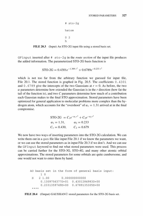
P1: OTA/XYZ P2: ABCc20 JWBS043-Rogers September 13, 2010 11:29 Printer Name: Yet to Come
STORED PARAMETERS 327
# sto-2g
hatom
0 2h
FILE 20.3 (Input) An STO-2G input file using a stored basis set.
GFinput inserted after # sto-2g in the route section of the input file producesthe added information. The parameterized STO-2G basis function is
STO-2G = 0.4301e−1.309 r2 + 0.6789e−0.233 r2
which is not too far from the arbitrary function we guessed for input file,File 20.1. The stored function is graphed in Fig. 20.5. The coefficients 0.4301and 0.6789 give the intercepts of the two Gaussians at r = 0. As before, the twoα parameters determine how extended the Gaussian is in the r direction (how fat thetail of the function is), and two C parameters determine how much of a contributioneach Gaussian makes to the final STO approximation. Stored parameters have beenoptimized for general application to molecular problems more complex than the hy-drogen atom, which accounts for the “overshoot” of α1 = 1.31 arrived at in the finalcompromise.
STO-2G = C1e−α1 r2 + C2e−α2 r2
α1 = 1.31, α2 = 0.233
C1 = 0.430, C2 = 0.679
We now have two ways of inserting parameters into the STO-2G calculation. We canwrite them out in a gen file like input File 20.1 if we know the parameters we want,or we can use the stored parameters as in input File 20.3 if we don’t. And we can usethe GFInput keyword to find out what stored parameters were used. This processcan be carried further for the STO-3G, STO-4G, and many other atomic orbitalapproximations. The stored parameters for some orbitals are quite cumbersome, andone would not want to enter them by hand.
AO basis set in the form of general basis input:1 0
S 2 1.00 0.0000000000000.1309756377D+01 0.4301284983D+000.2331359749D+00 0.6789135305D+00
****
FILE 20.4 (Output) GAUSSIAN C© stored parameters for the STO-2G basis set.
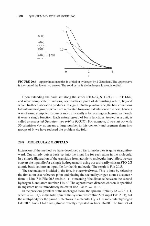
P1: OTA/XYZ P2: ABCc20 JWBS043-Rogers September 13, 2010 11:29 Printer Name: Yet to Come
328 QUANTUM MOLECULAR MODELING
20 4
0.5
1
(r)
1(r)
2(r)
1(r) 2(r)
r
FIGURE 20.6 Approximation to the 1s orbital of hydrogen by 2 Gaussians. The upper curveis the sum of the lower two curves. The solid curve is the hydrogen 1s atomic orbital.
Upon extending the basis set along the series STO-2G, STO-3G, . . . , STO-6G,and more complicated functions, one reaches a point of diminishing return, beyondwhich further elaboration produces little gain. On the positive side, the basis functionsfall into natural groups, which are replicated from one calculation to the next, hence away of using computer resources more efficiently is by treating each group as thoughit were a single function. Each natural group of basis functions, treated as a unit, iscalled a contracted Gaussian-type orbital (CGTO). For example, if we start out with36 primitives (by no means a large number in this context) and segment them intogroups of 6, we have reduced the problem six-fold.
20.8 MOLECULAR ORBITALS
Extension of the method we have developed so far to molecules is quite straightfor-ward. One simply puts a basis set into the input file for each atom in the molecule.In a simple illustration of the transition from atomic to molecular input files, we canconvert the input file for a single hydrogen atom using our arbitrarily chosen STO-2Gatomic basis set into an input file for the H2 molecule. The result is File 20.5.
The second atom is added to the first, in z-matrix format. This is done by selectingthe first atom as a reference point and placing the second hydrogen atom a distance rfrom it. Line 7 in File 20.5 reads h 1 r meaning “the distance between the secondhydrogen h and atom number 1 is r.” The approximate distance chosen is specifiedin angstrom units immediately below in line 9 as r = 0.7.
In the previous problem of the uncharged atom, the spin multiplicity M = 2S + 1,where S = ±1/2 is the total spin of the system, was 2 (line 5 of input File 20.3), butthe multiplicity for the paired σ electrons in molecular H2 is 1. In molecular hydrogenFile 20.5, lines 11–15 are (almost exactly) repeated in lines 16–20. The first set of
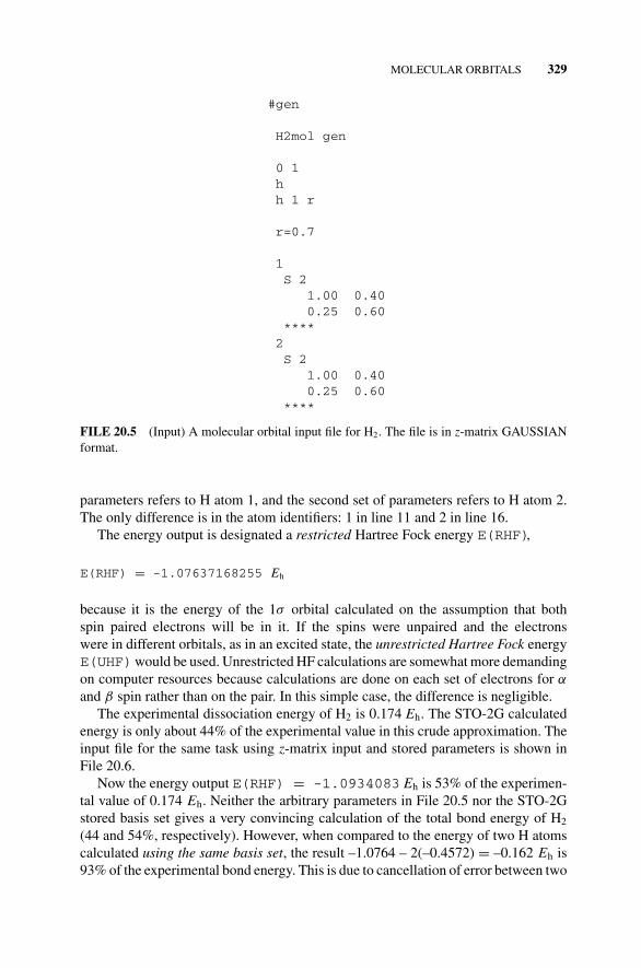
P1: OTA/XYZ P2: ABCc20 JWBS043-Rogers September 13, 2010 11:29 Printer Name: Yet to Come
MOLECULAR ORBITALS 329
#gen
H2mol gen
0 1hh 1 r
r=0.7
1S 2
1.00 0.400.25 0.60
****2S 2
1.00 0.400.25 0.60
****
FILE 20.5 (Input) A molecular orbital input file for H2. The file is in z-matrix GAUSSIANformat.
parameters refers to H atom 1, and the second set of parameters refers to H atom 2.The only difference is in the atom identifiers: 1 in line 11 and 2 in line 16.
The energy output is designated a restricted Hartree Fock energy E(RHF),
E(RHF) = -1.07637168255 Eh
because it is the energy of the 1σ orbital calculated on the assumption that bothspin paired electrons will be in it. If the spins were unpaired and the electronswere in different orbitals, as in an excited state, the unrestricted Hartree Fock energyE(UHF)would be used. Unrestricted HF calculations are somewhat more demandingon computer resources because calculations are done on each set of electrons for α
and β spin rather than on the pair. In this simple case, the difference is negligible.The experimental dissociation energy of H2 is 0.174 Eh. The STO-2G calculated
energy is only about 44% of the experimental value in this crude approximation. Theinput file for the same task using z-matrix input and stored parameters is shown inFile 20.6.
Now the energy output E(RHF) = -1.0934083 Eh is 53% of the experimen-tal value of 0.174 Eh. Neither the arbitrary parameters in File 20.5 nor the STO-2Gstored basis set gives a very convincing calculation of the total bond energy of H2
(44 and 54%, respectively). However, when compared to the energy of two H atomscalculated using the same basis set, the result –1.0764 – 2(–0.4572) = –0.162 Eh is93% of the experimental bond energy. This is due to cancellation of error between two

P1: OTA/XYZ P2: ABCc20 JWBS043-Rogers September 13, 2010 11:29 Printer Name: Yet to Come
330 QUANTUM MOLECULAR MODELING
# sto-2g
H2 molecule
0 1HH 1 rvariablesr=0.7
FILE 20.6 (Input) A GAUSSIAN input file for H2. The file is in z-matrix format.
systems: atom and molecule. Cancellation of error is often helpful but cannot be reliedupon. (Bear in mind that there is some uncertainty in the experimental value as well.)
20.8.1 GAMESS
GAMESS (General Atomic and Molecular Energy Structure System) is a molecularorbital program intended for general and academic use as open source software. Theauthors do not charge for this program, but the user may not sell it to anyone else.GAMESS gives the STO-2G energy calculated from input File 20.7. The geometryof the molecule is given in Cartesian coordinates. Only one nonzero coordinate isnecessary to designate the geometry of a diatomic linear molecule. The bond lengthis 0.7 A (estimated).
Translating File 20.7, each statement begins with $ and ends with $END. Thestatement may occupy more than one line. The $CONTROL statement specifies theSCFTYPe as RHF and the COORDinates as CARTesian $END. The $BASIS set isa Gaussian BASIS, which is STO and contains a Number of GAUSSians equal to2 $END. The $DATA set follows with an identifier Hydrogen for the human reader,the symmetry Dn1, and the coordinates in Cartesian format $END.
The single entry 0.7 A for the bond length is an element in the 2 × 3 matrix oflocations in Cartesian space using three components for each atom. One atom isplaced at the origin and the other is placed on the x axis at a distance of 0.7.
$CONTRL SCFTYP=RHF COORD=CART $END$BASIS GBASIS=STO NGAUSS=2 $END$DATA
HydrogenDn 1H 1.0 0.0 0.0 0.0H 1.0 0.7 0.0 0.0$END
FILE 20.7 (Input) GAMESS file for hydrogen molecule. The SCF calculation is RHF, thecoordinate system is Cartesian and the stored basis set is STO-2G. The symmetry space groupis Dn 1, the charge on each hydrogen atom is 1.0, and the bond length is 0.7 A.

P1: OTA/XYZ P2: ABCc20 JWBS043-Rogers September 13, 2010 11:29 Printer Name: Yet to Come
SPLIT VALENCE BASIS SETS 331
The energy, taken from a much more detailed output file, is
TOTAL ENERGY= -1.0934083240
The value calculated here used two Gaussian basis functions STO-2G and arrivedat an energy of −1.09340 Eh which replicates the output from File 20.6. The bondenergy BE is the difference between the molecular energy and the level of the atoms,which have an energy of 2(.5000):
BE = −1.0934 − 2 (−0.5000) = −0.0934 Eh = −245 kJ mol−1
This is about half of the experimental value of 435 kJ mol−1, slightly better thanthe one calculated using the estimated coefficients in File 20.5. Using six Gaussianfunctions improves the result to 0.0991 Eh = 260 kJ mol−1, which is about 57% ofthe experimental value:
TOTAL ENERGY= -1.0991105267
20.9 METHANE
The carbon atom can be combined with four hydrogen atoms to form input File 20.8for methane. The geometry for methane is given in approximate coordinates, whichwill be changed during the program run. Once carbon and hydrogen can be combined,the whole vista of alkanes, alkenes, and alkynes (many thousands of molecules) isopen. Extension to heteroatomic molecules other than hydrocarbons follows by thesame method (Example 20.1).
An optimized geometry is part of the output file. Neither the basis set nor theoptimized coordinate set is unique. Many (strictly, infinitely many) sets are possible.
Center Atomic Atomic Coordinates (Angstroms)Number Number Type X Y Z--------------------------------------------------------------
1 6 0 0.000000 0.000000 0.0001622 1 0 0.000000 0.000000 1.0890513 1 0 0.000000 1.026565 -0.3633404 1 0 -0.889032 -0.513283 -0.3633405 1 0 0.889032 -0.513283 -0.363340
FILE 20.8 One of many possible STO-2G optimized coordinate sets for methane. The carbonatom has been arbitrarily placed at the origin of a Cartesian coordinate system.
20.10 SPLIT VALENCE BASIS SETS
A hundred years of theory and experiment persuades us that the electrons in atomsreside in one or more “shells” surrounding the nucleus, each at a more or less fixed
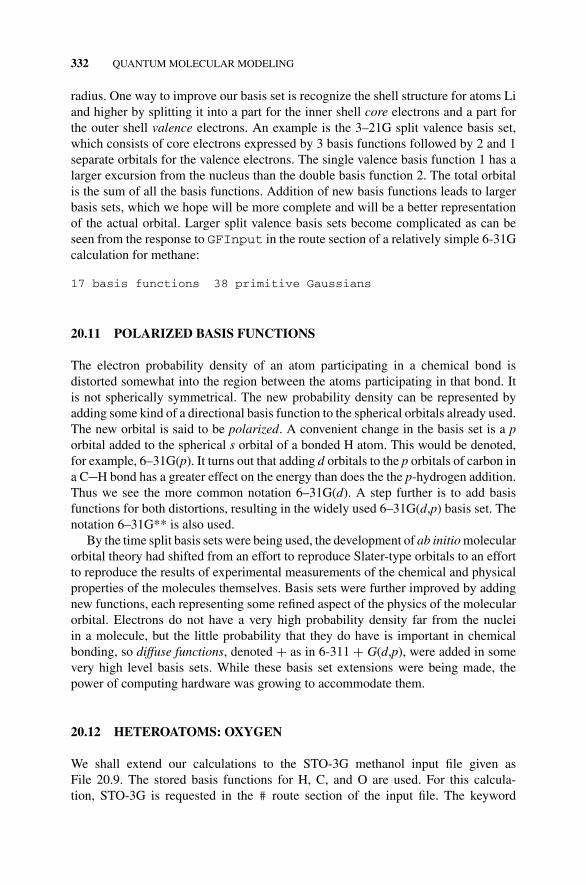
P1: OTA/XYZ P2: ABCc20 JWBS043-Rogers September 13, 2010 11:29 Printer Name: Yet to Come
332 QUANTUM MOLECULAR MODELING
radius. One way to improve our basis set is recognize the shell structure for atoms Liand higher by splitting it into a part for the inner shell core electrons and a part forthe outer shell valence electrons. An example is the 3–21G split valence basis set,which consists of core electrons expressed by 3 basis functions followed by 2 and 1separate orbitals for the valence electrons. The single valence basis function 1 has alarger excursion from the nucleus than the double basis function 2. The total orbitalis the sum of all the basis functions. Addition of new basis functions leads to largerbasis sets, which we hope will be more complete and will be a better representationof the actual orbital. Larger split valence basis sets become complicated as can beseen from the response to GFInput in the route section of a relatively simple 6-31Gcalculation for methane:
17 basis functions 38 primitive Gaussians
20.11 POLARIZED BASIS FUNCTIONS
The electron probability density of an atom participating in a chemical bond isdistorted somewhat into the region between the atoms participating in that bond. Itis not spherically symmetrical. The new probability density can be represented byadding some kind of a directional basis function to the spherical orbitals already used.The new orbital is said to be polarized. A convenient change in the basis set is a porbital added to the spherical s orbital of a bonded H atom. This would be denoted,for example, 6–31G(p). It turns out that adding d orbitals to the p orbitals of carbon ina C H bond has a greater effect on the energy than does the the p-hydrogen addition.Thus we see the more common notation 6–31G(d). A step further is to add basisfunctions for both distortions, resulting in the widely used 6–31G(d,p) basis set. Thenotation 6–31G** is also used.
By the time split basis sets were being used, the development of ab initio molecularorbital theory had shifted from an effort to reproduce Slater-type orbitals to an effortto reproduce the results of experimental measurements of the chemical and physicalproperties of the molecules themselves. Basis sets were further improved by addingnew functions, each representing some refined aspect of the physics of the molecularorbital. Electrons do not have a very high probability density far from the nucleiin a molecule, but the little probability that they do have is important in chemicalbonding, so diffuse functions, denoted + as in 6-311 + G(d,p), were added in somevery high level basis sets. While these basis set extensions were being made, thepower of computing hardware was growing to accommodate them.
20.12 HETEROATOMS: OXYGEN
We shall extend our calculations to the STO-3G methanol input file given asFile 20.9. The stored basis functions for H, C, and O are used. For this calcula-tion, STO-3G is requested in the # route section of the input file. The keyword
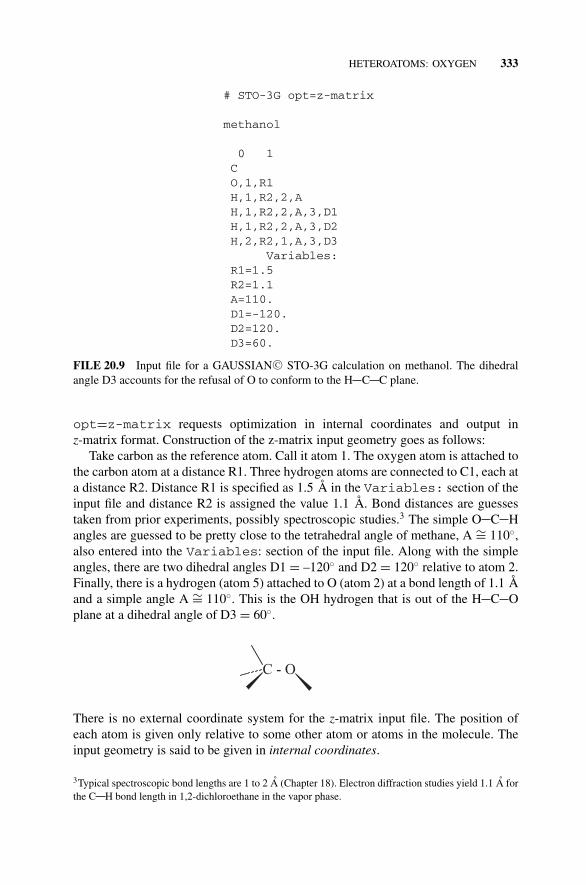
P1: OTA/XYZ P2: ABCc20 JWBS043-Rogers September 13, 2010 11:29 Printer Name: Yet to Come
HETEROATOMS: OXYGEN 333
# STO-3G opt=z-matrix
methanol
0 1CO,1,R1H,1,R2,2,AH,1,R2,2,A,3,D1H,1,R2,2,A,3,D2H,2,R2,1,A,3,D3
Variables:R1=1.5R2=1.1A=110.D1=-120.D2=120.D3=60.
FILE 20.9 Input file for a GAUSSIAN C© STO-3G calculation on methanol. The dihedralangle D3 accounts for the refusal of O to conform to the H C C plane.
opt=z-matrix requests optimization in internal coordinates and output inz-matrix format. Construction of the z-matrix input geometry goes as follows:
Take carbon as the reference atom. Call it atom 1. The oxygen atom is attached tothe carbon atom at a distance R1. Three hydrogen atoms are connected to C1, each ata distance R2. Distance R1 is specified as 1.5 A in the Variables: section of theinput file and distance R2 is assigned the value 1.1 A. Bond distances are guessestaken from prior experiments, possibly spectroscopic studies.3 The simple O C Hangles are guessed to be pretty close to the tetrahedral angle of methane, A ∼= 110◦,also entered into the Variables: section of the input file. Along with the simpleangles, there are two dihedral angles D1 = –120◦ and D2 = 120◦ relative to atom 2.Finally, there is a hydrogen (atom 5) attached to O (atom 2) at a bond length of 1.1 Aand a simple angle A ∼= 110◦. This is the OH hydrogen that is out of the H C Oplane at a dihedral angle of D3 = 60◦.
C - O
There is no external coordinate system for the z-matrix input file. The position ofeach atom is given only relative to some other atom or atoms in the molecule. Theinput geometry is said to be given in internal coordinates.
3Typical spectroscopic bond lengths are 1 to 2 A (Chapter 18). Electron diffraction studies yield 1.1 A forthe C H bond length in 1,2-dichloroethane in the vapor phase.
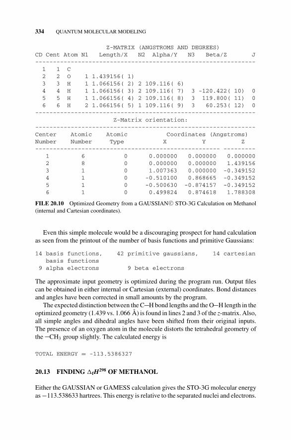
P1: OTA/XYZ P2: ABCc20 JWBS043-Rogers September 13, 2010 11:29 Printer Name: Yet to Come
334 QUANTUM MOLECULAR MODELING
Z-MATRIX (ANGSTROMS AND DEGREES)CD Cent Atom N1 Length/X N2 Alpha/Y N3 Beta/Z J--------------------------------------------------------------
1 1 C2 2 O 1 1.439156( 1)3 3 H 1 1.066156( 2) 2 109.116( 6)4 4 H 1 1.066156( 3) 2 109.116( 7) 3 -120.422( 10) 05 5 H 1 1.066156( 4) 2 109.116( 8) 3 119.800( 11) 06 6 H 2 1.066156( 5) 1 109.116( 9) 3 60.253( 12) 0
--------------------------------------------------------------Z-Matrix orientation:
--------------------------------------------------------------Center Atomic Atomic Coordinates (Angstroms)Number Number Type X Y Z---------------------------------------------------- ---------
1 6 0 0.000000 0.000000 0.0000002 8 0 0.000000 0.000000 1.4391563 1 0 1.007363 0.000000 -0.3491524 1 0 -0.510100 0.868665 -0.3491525 1 0 -0.500630 -0.874157 -0.3491526 1 0 0.499824 0.874618 1.788308
FILE 20.10 Optimized Geometry from a GAUSSIAN C© STO-3G Calculation on Methanol(internal and Cartesian coordinates).
Even this simple molecule would be a discouraging prospect for hand calculationas seen from the printout of the number of basis functions and primitive Gaussians:
14 basis functions, 42 primitive gaussians, 14 cartesianbasis functions
9 alpha electrons 9 beta electrons
The approximate input geometry is optimized during the program run. Output filescan be obtained in either internal or Cartesian (external) coordinates. Bond distancesand angles have been corrected in small amounts by the program.
The expected distinction between the C H bond lengths and the O H length in theoptimized geometry (1.439 vs. 1.066 A) is found in lines 2 and 3 of the z-matrix. Also,all simple angles and dihedral angles have been shifted from their original inputs.The presence of an oxygen atom in the molecule distorts the tetrahedral geometry ofthe CH3 group slightly. The calculated energy is
TOTAL ENERGY = -113.5386327
20.13 FINDING fH298 OF METHANOL
Either the GAUSSIAN or GAMESS calculation gives the STO-3G molecular energyas −113.538633 hartrees. This energy is relative to the separated nuclei and electrons.
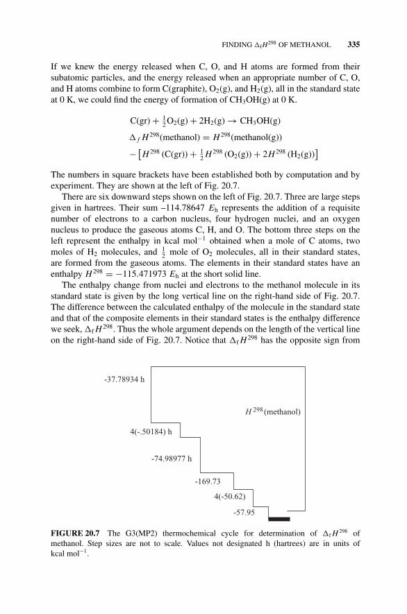
P1: OTA/XYZ P2: ABCc20 JWBS043-Rogers September 13, 2010 11:29 Printer Name: Yet to Come
FINDING fH298 OF METHANOL 335
If we knew the energy released when C, O, and H atoms are formed from theirsubatomic particles, and the energy released when an appropriate number of C, O,and H atoms combine to form C(graphite), O2(g), and H2(g), all in the standard stateat 0 K, we could find the energy of formation of CH3OH(g) at 0 K.
C(gr) + 12 O2(g) + 2H2(g) → CH3OH(g)
f H 298(methanol) = H 298(methanol(g))
− [H 298 (C(gr)) + 1
2 H 298 (O2(g)) + 2H 298 (H2(g))]
The numbers in square brackets have been established both by computation and byexperiment. They are shown at the left of Fig. 20.7.
There are six downward steps shown on the left of Fig. 20.7. Three are large stepsgiven in hartrees. Their sum –114.78647 Eh represents the addition of a requisitenumber of electrons to a carbon nucleus, four hydrogen nuclei, and an oxygennucleus to produce the gaseous atoms C, H, and O. The bottom three steps on theleft represent the enthalpy in kcal mol−1 obtained when a mole of C atoms, twomoles of H2 molecules, and 1
2 mole of O2 molecules, all in their standard states,are formed from the gaseous atoms. The elements in their standard states have anenthalpy H 298 = −115.471973 Eh at the short solid line.
The enthalpy change from nuclei and electrons to the methanol molecule in itsstandard state is given by the long vertical line on the right-hand side of Fig. 20.7.The difference between the calculated enthalpy of the molecule in the standard stateand that of the composite elements in their standard states is the enthalpy differencewe seek, f H 298. Thus the whole argument depends on the length of the vertical lineon the right-hand side of Fig. 20.7. Notice that f H 298 has the opposite sign from
-37.78934 h
4(-.50184) h
-74.98977 h
-169.73
4(-50.62)
-57.95
H 298(methanol)
FIGURE 20.7 The G3(MP2) thermochemical cycle for determination of f H 298 ofmethanol. Step sizes are not to scale. Values not designated h (hartrees) are in units ofkcal mol−1.
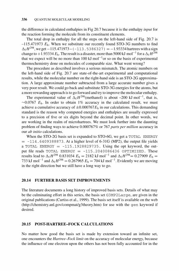
P1: OTA/XYZ P2: ABCc20 JWBS043-Rogers September 13, 2010 11:29 Printer Name: Yet to Come
336 QUANTUM MOLECULAR MODELING
the difference in calculated enthalpies in Fig 20.7 because it is the enthalpy input forthe reaction forming the molecule from its constituent elements.
The total drop in enthalpy for all the steps on the left-hand side of Fig. 20.7 is–115.471973 Eh. When we substitute our recently found STO-3G numbers to find f H 298, we get −115.471973 –(-113.5386327)=−1.93334 hartrees with a signchange to +1.93334 Eh. The result is a disaster, more than 5000 kJ mol−1 for a f H 298
that we expect will be no more than 100 kJ mol−1or so on the basis of experimentalthermochemistry done on molecules of comparable size. What went wrong?
The procedure as described involves a serious mismatch. The atomic numbers onthe left-hand side of Fig. 20.7 are state-of-the-art experimental and computationalresults, while the molecular number on the right-hand side is an STO-2G approxima-tion. A large approximate number subtracted from a large accurate number gives avery poor result. We could go back and substitute STO-3G energies for the atoms, buta more rewarding approach is to go forward and try to improve the molecular enthalpy.
The experimental value of f H 298(methanol) is about –200 kJ mol−1, that is,∼0.0767 Eh. In order to obtain 1% accuracy in the calculated result, we mustachieve a cumulative accuracy of ±0.000767Eh in our calculations. This demandingstandard is the reason why computed energies and enthalpies are usually expressedto a precision of five or six digits beyond the decimal point. In other words, weare working in the realm of microhartrees. We must look further into the dauntingproblem of finding ways to achieve 0.000767% or 767 parts per million accuracy inour ab initio calculations.
When the STO-2G basis set is expanded to STO-6G, we get a TOTAL ENERGY= -114.6409388873. At a higher level of 6-31G (MP2), the output file yieldsa TOTAL ENERGY = -115.1928829735. Using the opt keyword, the out-put file reads TOTAL ENERGY = -115.2040086436 OPTIMIZED. Theseresults lead to f H 298 0.831034 Eh = 2182 kJ mol−1 and f H 298= 0.27909 Eh =733 kJ mol−1 and f H 298 = 0.267965 Eh = 704 kJ mol−1. Evidently we are movingin the right direction but we still have a long way to go.
20.14 FURTHER BASIS SET IMPROVEMENTS
The literature documents a long history of improved basis sets. Details of what maybe the culminating effort in this series, the basis set G3MP2Large, are given in theoriginal publications (Curtiss et al., 1999). The basis set itself is available on the web(http://chemistry.anl.gov/compmat/g3theory.htm) for use with the gen keyword ifdesired.
20.15 POST-HARTREE–FOCK CALCULATIONS
No matter how good the basis set is made by extension toward an infinite set,one encounters the Hartree–Fock limit on the accuracy of molecular energy, becausethe influence of one electron upon the others has not been fully accounted for in the
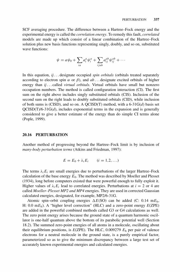
P1: OTA/XYZ P2: ABCc20 JWBS043-Rogers September 13, 2010 11:29 Printer Name: Yet to Come
PERTURBATION 337
SCF averaging procedure. The difference between a Hartree–Fock energy and theexperimental energy is called the correlation energy. To remedy this fault, correlatedmodels are made up which consist of a linear combination of the Hartree–Focksolution plus new basis functions representing singly, doubly, and so on, substitutedwave functions:
ψ = aψ0 +∑
ia
aai ψa
i +∑i jab
aabi j ψab
i j + · · ·
In this equation, ij . . . designate occupied spin orbitals (orbitals treated separatelyaccording to electron spin α or β), and ab . . . designate excited orbitals of higherenergy than ij . . . called virtual orbitals. Virtual orbitals have small but nonzerooccupation numbers. The method is called configuration interaction (CI). The firstsum on the right above includes singly substituted orbitals (CIS). Inclusion of thesecond sum on the right leads to doubly substituted orbitals (CID), while inclusionof both sums is (CISD), and so on. A QCISD(T) method, with a 6-31G(d) basis setQCISD(T)/6-31G(d), includes exponential terms in the expansion and is generallyconsidered to give a better estimate of the energy than do simple CI terms alone(Pople, 1999).
20.16 PERTURBATION
Another method of progressing beyond the Hartree–Fock limit is by inclusion ofmany-body perturbation terms (Atkins and Friedman, 1997):
E = E0 + λi Ei (i = 1,2, . . .)
The terms λi Ei are small energies due to perturbations of the larger Hartree–Fockcalculation of the base energy E0. The method was described by Moeller and Plesset(1934), long before computers existed that were powerful enough to fully exploit it.Higher values of λi Ei lead to correlated energies. Perturbations at i = 2 or 4 arecalled Moeller–Plesset MP2 and MP4 energies. They are used in corrected Gaussiancalculated energies, designated, for example, MP2/6-31G.
Atomic spin–orbit coupling energies E(SO) can be added (C: 0.14 mEh,H: 0.0 mEh). A “higher level correction” (HLC) and a zero-point energy E(ZPE)are added in the powerful combined methods called G3 or G4 calculations as well.The zero point energy arises because the ground state of a quantum harmonic oscil-lator is one-half quantum above the bottom of its parabolic potential well (Section18.2). The summed zero-point energies of all atoms in a molecule, oscillating abouttheir equilibrium positions, is E(ZPE). The HLC, 0.009279 Eh per pair of valenceelectrons for a neutral molecule in the ground state, is a purely empirical factor,parameterized so as to give the minimum discrepancy between a large test set ofaccurately known experimental energies and calculated energies.
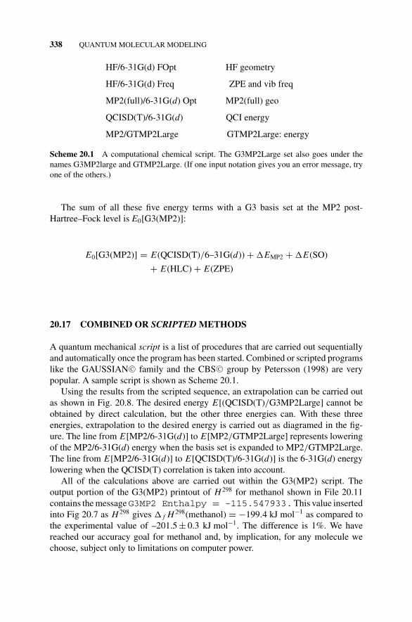
P1: OTA/XYZ P2: ABCc20 JWBS043-Rogers September 13, 2010 11:29 Printer Name: Yet to Come
338 QUANTUM MOLECULAR MODELING
HF/6-31G(d) FOpt HF geometry
HF/6-31G(d) Freq ZPE and vib freq
MP2(full)/6-31G(d) Opt MP2(full) geo
QCISD(T)/6-31G(d) QCI energy
MP2/GTMP2Large GTMP2Large: energy
Scheme 20.1 A computational chemical script. The G3MP2Large set also goes under thenames G3MP2large and GTMP2Large. (If one input notation gives you an error message, tryone of the others.)
The sum of all these five energy terms with a G3 basis set at the MP2 post-Hartree–Fock level is E0[G3(MP2)]:
E0[G3(MP2)] = E(QCISD(T)/6–31G(d)) + EMP2 + E(SO)
+ E(HLC) + E(ZPE)
20.17 COMBINED OR SCRIPTED METHODS
A quantum mechanical script is a list of procedures that are carried out sequentiallyand automatically once the program has been started. Combined or scripted programslike the GAUSSIAN C© family and the CBS C© group by Petersson (1998) are verypopular. A sample script is shown as Scheme 20.1.
Using the results from the scripted sequence, an extrapolation can be carried outas shown in Fig. 20.8. The desired energy E[(QCISD(T)/G3MP2Large] cannot beobtained by direct calculation, but the other three energies can. With these threeenergies, extrapolation to the desired energy is carried out as diagramed in the fig-ure. The line from E[MP2/6-31G(d)] to E[MP2/GTMP2Large] represents loweringof the MP2/6-31G(d) energy when the basis set is expanded to MP2/GTMP2Large.The line from E[MP2/6-31G(d)] to E[QCISD(T)/6-31G(d)] is the 6-31G(d) energylowering when the QCISD(T) correlation is taken into account.
All of the calculations above are carried out within the G3(MP2) script. Theoutput portion of the G3(MP2) printout of H 298 for methanol shown in File 20.11contains the messageG3MP2 Enthalpy = -115.547933.This value insertedinto Fig 20.7 as H 298 gives f H 298(methanol) = −199.4 kJ mol−1 as compared tothe experimental value of –201.5 ± 0.3 kJ mol−1. The difference is 1%. We havereached our accuracy goal for methanol and, by implication, for any molecule wechoose, subject only to limitations on computer power.
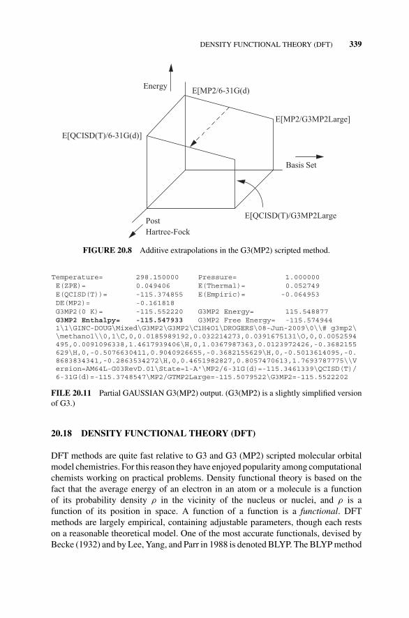
P1: OTA/XYZ P2: ABCc20 JWBS043-Rogers September 13, 2010 11:29 Printer Name: Yet to Come
DENSITY FUNCTIONAL THEORY (DFT) 339
E[MP2/6-31G(d)
E[MP2/G3MP2Large]
E[QCISD(T)/6-31G(d)]
PostHartree-Fock
Basis Set
Energy
E[QCISD(T)/G3MP2Large
FIGURE 20.8 Additive extrapolations in the G3(MP2) scripted method.
Temperature= 298.150000 Pressure= 1.000000 E(ZPE)= 0.049406 E(Thermal)= 0.052749 E(QCISD(T))= -115.374855 E(Empiric)= -0.064953 DE(MP2)= -0.161818 G3MP2(0 K)= -115.552220 G3MP2 Energy= 115.548877 G3MP2 Enthalpy= -115.547933 G3MP2 Free Energy= -115.574944 1\1\GINC-DOUG\Mixed\G3MP2\G3MP2\C1H4O1\DROGERS\08-Jun-2009\0\\# g3mp2\ \methanol\\0,1\C,0,0.0185989192,0.032214273,0.0391675131\O,0,0.0052594 495,0.0091096338,1.4617939406\H,0,1.0367987363,0.0123972426,-0.3682155 629\H,0,-0.5076630411,0.9040926655,-0.3682155629\H,0,-0.5013614095,-0. 8683834341,-0.2863534272\H,0,0.4651982827,0.8057470613,1.7693787775\\V ersion=AM64L-G03RevD.01\State=1-A'\MP2/6-31G(d)=-115.3461339\QCISD(T)/ 6-31G(d)=-115.3748547\MP2/GTMP2Large=-115.5079522\G3MP2=-115.5522202
FILE 20.11 Partial GAUSSIAN G3(MP2) output. (G3(MP2) is a slightly simplified versionof G3.)
20.18 DENSITY FUNCTIONAL THEORY (DFT)
DFT methods are quite fast relative to G3 and G3 (MP2) scripted molecular orbitalmodel chemistries. For this reason they have enjoyed popularity among computationalchemists working on practical problems. Density functional theory is based on thefact that the average energy of an electron in an atom or a molecule is a functionof its probability density ρ in the vicinity of the nucleus or nuclei, and ρ is afunction of its position in space. A function of a function is a functional. DFTmethods are largely empirical, containing adjustable parameters, though each restson a reasonable theoretical model. One of the most accurate functionals, devised byBecke (1932) and by Lee, Yang, and Parr in 1988 is denoted BLYP. The BLYP method
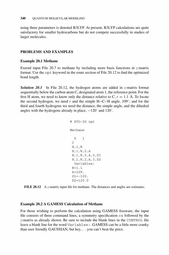
P1: OTA/XYZ P2: ABCc20 JWBS043-Rogers September 13, 2010 11:29 Printer Name: Yet to Come
340 QUANTUM MOLECULAR MODELING
using three parameters is denoted B3LYP. At present, B3LYP calculations are quitesatisfactory for smaller hydrocarbons but do not compete successfully in studies oflarger molecules.
PROBLEMS AND EXAMPLES
Example 20.1 Methane
Extend input File 20.7 to methane by including more basis functions in z-matrixformat. Use the opt keyword in the route section of File 20.12 to find the optimizedbond length.
Solution 20.1 In File 20.12, the hydrogen atoms are added in z-matrix formatsequentially below the carbon atom C, designated atom 1, the reference point. For thefirst H atom, we need to know only the distance relative to C, r = 1.1 A. To locatethe second hydrogen, we need r and the simple H C H angle, 109◦; and for thethird and fourth hydrogens we need the distance, the simple angle, and the dihedralangles with the hydrogens already in place, −120◦ and 120◦.
# STO-2G opt
Methane
0 1CH,1,RH,1,R,2,AH,1,R,2,A,3,D1H,1,R,2,A,3,D2Variables:
R=1.1A=109.D1=-120.D2=120.0
FILE 20.12 A z-matrix input file for methane. The distances and angles are estimates.
Example 20.2 A GAMESS Calculation of Methane
For those wishing to perform the calculation using GAMESS freeware, the inputfile consists of three command lines, a symmetry specification cs followed by thez-matrix as already shown. Be sure to include the blank lines in the CONTROL fileleave a blank line for the word Variables:. GAMESS can be a little more crankythan user friendly GAUSSIAN, but hey, . . . you can’t beat the price.
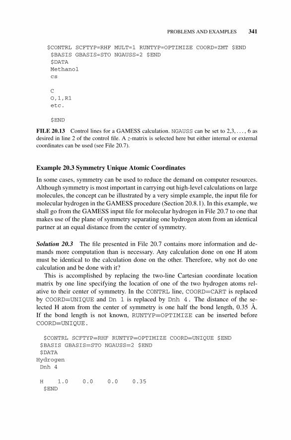
P1: OTA/XYZ P2: ABCc20 JWBS043-Rogers September 13, 2010 11:29 Printer Name: Yet to Come
PROBLEMS AND EXAMPLES 341
$CONTRL SCFTYP=RHF MULT=1 RUNTYP=OPTIMIZE COORD=ZMT $END$BASIS GBASIS=STO NGAUSS=2 $END$DATAMethanolcs
CO,1,R1etc.
$END
FILE 20.13 Control lines for a GAMESS calculation. NGAUSS can be set to 2,3, . . . , 6 asdesired in line 2 of the control file. A z-matrix is selected here but either internal or externalcoordinates can be used (see File 20.7).
Example 20.3 Symmetry Unique Atomic Coordinates
In some cases, symmetry can be used to reduce the demand on computer resources.Although symmetry is most important in carrying out high-level calculations on largemolecules, the concept can be illustrated by a very simple example, the input file formolecular hydrogen in the GAMESS procedure (Section 20.8.1). In this example, weshall go from the GAMESS input file for molecular hydrogen in File 20.7 to one thatmakes use of the plane of symmetry separating one hydrogen atom from an identicalpartner at an equal distance from the center of symmetry.
Solution 20.3 The file presented in File 20.7 contains more information and de-mands more computation than is necessary. Any calculation done on one H atommust be identical to the calculation done on the other. Therefore, why not do onecalculation and be done with it?
This is accomplished by replacing the two-line Cartesian coordinate locationmatrix by one line specifying the location of one of the two hydrogen atoms rel-ative to their center of symmetry. In the CONTRL line, COORD=CART is replacedby COORD=UNIQUE and Dn 1 is replaced by Dnh 4. The distance of the se-lected H atom from the center of symmetry is one half the bond length, 0.35 A.If the bond length is not known, RUNTYP=OPTIMIZE can be inserted beforeCOORD=UNIQUE.
$CONTRL SCFTYP=RHF RUNTYP=OPTIMIZE COORD=UNIQUE $END$BASIS GBASIS=STO NGAUSS=2 $END$DATA
HydrogenDnh 4
H 1.0 0.0 0.0 0.35$END

P1: OTA/XYZ P2: ABCc20 JWBS043-Rogers September 13, 2010 11:29 Printer Name: Yet to Come
342 QUANTUM MOLECULAR MODELING
The energy output of this simplified file is the same as the more complicatedFile 20.7.
TOTAL ENERGY = -1.0934083240
Optimizing from a bond length estimate that is 10% in error leads to
E = -1.0938179551
which is different by about 0.25 kcal mol−1 (slightly lower).
Problem 20.1
Find the energy of a particle in a one-dimensional box of length l. by the variationalmethod. Take �(x) = A sin nπx/ l as a trial function. Note that the Hamiltonian is−(�2/2m)(∂2/∂x2).
Problem 20.2
Electron diffraction studies yield two different Cl Cl distances (not bonded) in 1,2-dichloroethane CH2Cl CH2Cl. Explain why this is so. What influence does this facthave on molecular structure and energy calculations like MM and G3(MP2)?
Problem 20.3
The benzene molecule can be modeled as a potential well with a square planar bottom0.400 nm on each side containing six 2pπ electrons (ignoring all the other electronsin the molecule). What is the degeneracy of the occupied orbitals and what is thedegeneracy of the first two virtual orbitals according to this model? In what respectdoes this model fail to represent the true levels of the benzene molecule?
Problem 20.4
Given the model proposed in Problem 20.3, what is the minimum energy required topromote a ground state electron to its first excited state? What is the wavelength ofelectromagnetic radiation that will supply this energy? Is this in the visible region?Is benzene colored?
Problem 20.5
(a) Add a basis function of your own to the STO-2G basis set so as to createyour personal STO-3G linear combination. Use a graphing program to plotyour function, call it ϕmySTO-3G = f (r ). STO-3G calculations were used atthe research level until the 1990s.
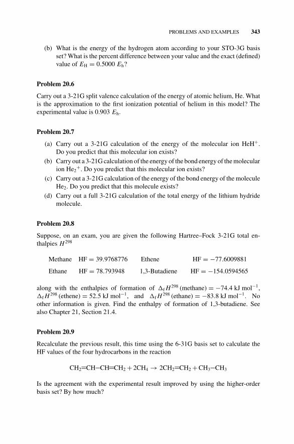
P1: OTA/XYZ P2: ABCc20 JWBS043-Rogers September 13, 2010 11:29 Printer Name: Yet to Come
PROBLEMS AND EXAMPLES 343
(b) What is the energy of the hydrogen atom according to your STO-3G basisset? What is the percent difference between your value and the exact (defined)value of EH = 0.5000 Eh?
Problem 20.6
Carry out a 3-21G split valence calculation of the energy of atomic helium, He. Whatis the approximation to the first ionization potential of helium in this model? Theexperimental value is 0.903 Eh.
Problem 20.7
(a) Carry out a 3-21G calculation of the energy of the molecular ion HeH+.Do you predict that this molecular ion exists?
(b) Carry out a 3-21G calculation of the energy of the bond energy of the molecularion He2
+. Do you predict that this molecular ion exists?
(c) Carry out a 3-21G calculation of the energy of the bond energy of the moleculeHe2. Do you predict that this molecule exists?
(d) Carry out a full 3-21G calculation of the total energy of the lithium hydridemolecule.
Problem 20.8
Suppose, on an exam, you are given the following Hartree–Fock 3-21G total en-thalpies H 298
Methane HF = 39.9768776 Ethene HF = −77.6009881
Ethane HF = 78.793948 1,3-Butadiene HF = −154.0594565
along with the enthalpies of formation of f H 298 (methane) = −74.4 kJ mol−1, f H 298 (ethene) = 52.5 kJ mol−1, and f H 298 (ethane) = −83.8 kJ mol−1. Noother information is given. Find the enthalpy of formation of 1,3-butadiene. Seealso Chapter 21, Section 21.4.
Problem 20.9
Recalculate the previous result, this time using the 6-31G basis set to calculate theHF values of the four hydrocarbons in the reaction
CH2 CH CH CH2 + 2CH4 → 2CH2 CH2 + CH3 CH3
Is the agreement with the experimental result improved by using the higher-orderbasis set? By how much?
P1: OTA/XYZ P2: ABCc21 JWBS043-Rogers September 13, 2010 11:30 Printer Name: Yet to Come
21PHOTOCHEMISTRY AND THETHEORY OF CHEMICAL REACTIONS
So far we have considered chemical reactions in which the energy necessary tosurmount the activation barrier is obtained from the environment in the form of heattranslated as molecular motion. These are thermal reactions. Light of frequency ν isalso able to impart energy E = hν to reactant molecules so that they can surmountthe barrier. These are photochemical reactions.
21.1 EINSTEIN’S LAW
Like any chemical reaction, a photochemical reaction involves excitation of thereactant species up and over an activation energy barrier before transmission tothe product state. In a photochemical reaction, the activation energy is supplied byincident light instead of ambient heat. The Bohr–Einstein concept of a particle oflight (a photon) carrying a quantum of energy E = hν leads one to suppose that theenergy of an incident light particle is concentrated in one reactant molecule only,rather than being distributed evenly over an entire collection of molecules. Thismechanism of energy transmission means that if the quantum E is sufficiently large,all struck molecules will acquire the activation energy and the number of moleculesreacting will be equal to the number of photons striking and retained by the system.This is Einstein’s law.
molecules reacting = photons absorbed
Concise Physical Chemistry, by Donald W. RogersCopyright C© 2011 John Wiley & Sons, Inc.
344
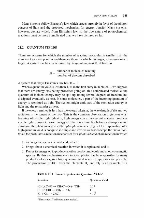
P1: OTA/XYZ P2: ABCc21 JWBS043-Rogers September 13, 2010 11:30 Printer Name: Yet to Come
QUANTUM YIELDS 345
Many systems follow Einstein’s law, which argues strongly in favor of the photonconcept of light and the proposed mechanism for energy transfer. Many systems,however, deviate widely from Einstein’s law, so the true nature of photochemicalreactions must be more complicated than we have pictured so far.
21.2 QUANTUM YIELDS
There are systems for which the number of reacting molecules is smaller than thenumber of incident photons and there are those for which it is larger, sometimes muchlarger. A system can be characterized by its quantum yield �, defined as
� = number of molecules reacting
number of photons absorbed
A system that obeys Einstein’s law has � = 1.When a quantum yield is less than 1, as in the first entry in Table 21.1, we suppose
that there are energy dissipating processes going on. In a complicated molecule, thequantum of incident energy may be split up among several degrees of freedom anddissipated eventually as heat. In some molecules, a part of the incoming quantum ofenergy is reemitted as light. The system might emit part of the excitation energy aslight and the remainder as heat.
If the energy emitted is less than the energy taken in, the wavelength of the emittedradiation is the longer of the two. This is the common observation in fluorescence;beaming ultraviolet light (short λ, high energy) on a fluorescent material producesvisible light (longer λ, lower energy). If there is a time lag between absorption andemission, the phenomenon is called phosphorescence (Fig. 21.1). Explanation of ahigh quantum yield is not quite so simple and involves a new concept, the chain reac-tion. One postulates a reaction mechanism for a photoinduced chain reaction in which
1. an energetic species is produced, which
2. brings about a chemical reaction in which it is replicated, and it
3. Passes its energy on to produce another product molecule and another energeticspecies. By this mechanism, each incident photon can be responsible for manyproduct molecules, so a high quantum yield results. Explosions are possible.The production of HCl from the elements H2 and Cl2 is an example of a
TABLE 21.1 Some Experimental Quantum Yieldsa.
Reaction Quantum Yield
(CH3)2C O → CH3C• O + •CH3 0.17CH3COOH → CH4 + CO2 1H2 + Cl2 → 2HCl ∼105
aThe symbol • indicates a free radical.
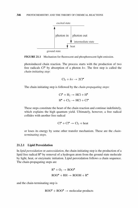
P1: OTA/XYZ P2: ABCc21 JWBS043-Rogers September 13, 2010 11:30 Printer Name: Yet to Come
346 PHOTOCHEMISTRY AND THE THEORY OF CHEMICAL REACTIONS
ground state
intermediate state
excited state
photon in photon out
heat
FIGURE 21.1 Mechanism for fluorescent and phosphorescent light emission.
photoinduced chain reaction. The process starts with the production of twofree radicals Cl• by absorption of a photon hν. The first step is called thechain-initiating step:
Cl2 + hν → 2Cl•
The chain initiating step is followed by the chain-propagating steps:
Cl• + H2 → HCl + H•
H• + Cl2 → HCl + Cl•
These steps constitute the heart of the chain reaction and continue indefinitely,which explains the high quantum yield. Ultimately, however, a free radicalcollides with another free radical
Cl• + Cl• → Cl2 + heat
or loses its energy by some other transfer mechanism. These are the chain-terminating steps.
21.2.1 Lipid Peroxidation
In lipid peroxidation or autooxidation, the chain-initiating step is the production of alipid free radical R• by removal of a hydrogen atom from the ground state moleculeby light, heat, or enzymatic initiation. Lipid peroxidation follows a chain sequence.The chain-propagating steps are
R• + O2 → ROO•
ROO• + RH → ROOH + R•
and the chain-terminating step is
ROO• + ROO• → molecular products
P1: OTA/XYZ P2: ABCc21 JWBS043-Rogers September 13, 2010 11:30 Printer Name: Yet to Come
QUANTUM YIELDS 347
This chain reaction is damaging to biological membranes, especially cell walls, andhas been implicated in both carcinogenesis and the aging process. Within livingsystems, the unsaturated fatty acids are most vulnerable to autooxidation.
Living biological systems (as contrasted to dead ones) are protected from thisautooxidation process through the action of small amounts of exogenous antioxidants,including vitamin E. Antioxidants form very reactive free radicals themselves. Theseradicals interfere with the chain oxygenation cycle in the propagation steps by reactingwith the radical ROO•. This terminates the chain and limits damage to the organism.Vitamin E is the name given to the group of four tocopherols. The tocopherols arearomatic alcohols ArOH, which react with peroxyl radicals.
ROO• + ArOH → ROOH + ArO•
The phenol radical ArO• is stabilized by delocalization of electrons over the aromaticframework. Because of their stability, they persist in the system and eventually reactwith a peroxyl radical to complete the chain-breaking mechanism
ArO• + ROO• → products
21.2.2 Ozone Depletion
Neither O nor O2 absorbs radiation in the 200- to 300-nm (ultraviolet) region, butozone O3 absorbs at about 250 nm, shielding the earth’s surface and creatures livingon it from mutagenic DNA alteration by impact of ultraviolet photons. Among themany photochemical reactions occurring in the earth’s stratosphere is a sequence inwhich the middle two reactions below are in balance, maintaining a low but fairlyconstant ozone level.
O2 + hν (< 200 nm) → 2O
O3 + hν(UV ) → O2 + O
O + O2 + M →← O3 + M
O + O3 → 2O2
M is a molecule, possibly N2, that does not enter into the reaction but exchangesenergy through collisions with those that do.
Other reactions interfere with this cycle, hence they interfere with the stratosphericozone level. An example is the chlorine cycle involving Cl2O2 derived ultimately fromman-made chlorofluorocarbons. Stratospheric chlorine has increased by a factor ofabout 7 in the past 50 years, and a decrease in stratospheric ozone has been found(primarily for reasons of atmospheric turbulence) over Antarctica. This is the sourceof the polar “ozone hole.” There is no reason to suppose that ozone depletion, thoughit is most easily monitored over the poles, is limited to the polar stratosphere.
P1: OTA/XYZ P2: ABCc21 JWBS043-Rogers September 13, 2010 11:30 Printer Name: Yet to Come
348 PHOTOCHEMISTRY AND THE THEORY OF CHEMICAL REACTIONS
21.3 BOND DISSOCIATION ENERGIES (BDE)
In photoinduced and many other mechanisms, we are concerned with the stabilityand rate of formation of free radicals, for example,
CH4 → CH•3 + H•
The enthalpy of homolytic cleavage is not easy to measure for these fleeting species,but they can be calculated as an ordinary dissociation:
AB → A• + B•
The bond dissociation energy BDE of ethane
CH3CH3 → CH•3 + CH•
3
to produce methyl radicals is a simple example of the more general case for hydro-carbons and their radicals:
CH3R → CH•3 + R•
BDE [CH3R] = �f H298[CH•
3
] + �f H298 [R•] − �f H298 [CH3R]
The radical R may be branched, or it may contain double or triple bonds, or it maycontain two or all three of these structural features (Rogers et al., 2006).
21.4 LASERS
Some atoms and molecules can undergo a population inversion, such that an upperenergy state is more highly populated than the ground state. When this happens,incident radiation is reemitted with its initial energy plus an energy gain obtained asthe gain medium returns to its ground state. In commercial lasers, atoms or moleculescomprising the gain medium are intentionally driven into a population inversion byan optical pump, which emits high-energy radiation or fast electrons.
A laser consists of an optical pump that brings about a population inversion in again medium which lases, bringing about a slight radiative amplification of the lightsource. The radiation from this laser gain medium is reflected back and forth betweentwo mirrors so that amplification is increased on each pass through the medium. Onemirror is intentionally made less reflective than the other so that some of the highlyamplified radiation passes through the less reflective mirror and is emitted as a laserbeam. Einstein developed the theory of lasers long before the first commercial laserwas produced.

P1: OTA/XYZ P2: ABCc21 JWBS043-Rogers September 13, 2010 11:30 Printer Name: Yet to Come
THE EYRING THEORY OF REACTION RATES 349
21.5 ISODESMIC REACTIONS
Ab initio enthalpy calculations of H 298 for hydrocarbons containing more than 2or 3 carbon atoms are often converted to thermodynamic values by setting up anisodesmic reaction in which an experimental �f H 298 is known for all participantsbut one (Hehre et al., 1970). The single remaining unknown �f H 298 is calculatedfrom the known experimental values by difference. Computed �f H 298 values forindividual molecules on the right and left of the equation may suffer considerableerror; but if the bond types are the same on both sides of the reaction, errors tendto cancel because they arise from similar computational defects. Isodesmic reactionsare usually set up such that a relatively complicated molecule is compared to severalsimple molecules like methane and ethane, for which the experimental values arethought to be very accurate.
21.6 THE EYRING THEORY OF REACTION RATES
Henry Eyring (1935) worked out a theory of reaction rates, which explains theArrhenius law of temperature dependence and which leads to a conceptual picturethat has been widely used in many branches of chemistry. In Section 20.2, we basedour qualitative thinking about complicated molecules on the system of the hydrogenmolecule ion because it is the only molecule simple enough to describe completely.So we would like to base our thinking about complicated reaction mechanisms onthe simpler system of one hydrogen atom substituting for another1:
H + H − H → H − H + H
The attack of a hydrogen atom on a hydrogen molecule encounters an ellipsoidalrepulsive field with the minimum repulsion at either end of the molecule.
H H
Under the simplifying assumption that the attack of the hydrogen atom on H2 is anend-on attack, only two distances are necessary to describe the reacting system, thedistance from the the attacked hydrogen molecule to the incoming H, and the distancefrom the opposite end of the molecule to the outgoing H. Call these distances r ′
HH and
1Experimentally, deuterium atoms D were used because they can be distinguished from H by theirdifference in mass.

P1: OTA/XYZ P2: ABCc21 JWBS043-Rogers September 13, 2010 11:30 Printer Name: Yet to Come
350 PHOTOCHEMISTRY AND THE THEORY OF CHEMICAL REACTIONS
rHH. At some instant, the incoming H and the departing H must be equidistant fromthe central hydrogen atom so that the three atoms form an energetic intermediate:
H + H − H =⎡⎣H
r ′HH︷︸︸︷· · · H
rHH︷︸︸︷· · · H
⎤⎦ = H − H + H
The bond-forming configuration is on the left and the bond-breaking configuration ison the right of the central structure, which is the activated complex.
21.7 THE POTENTIAL ENERGY SURFACE
In the study of molecular structure, we plotted the potential energy of the molecule asa function of internuclear distance and found that it has a minimum at the equilibriumbond length. Some of the qualities of this potential energy curve carry over to theactivated complex, but now the potential energy is a more complicated function of twovariables r ′
HH and rHH. It requires a three-dimensional surface or a two-dimensionalcontour map for its representation. Eyring has constructed such a surface representedby the equivalent contour map in Fig. 21.2.
This contour map is drawn in the same way that a forest service map of WesternMontana would be drawn. Each contour corresponds to a constant potential energythat would occupy the dimension out of the plane of the paper if the three-dimensionalrepresentation were used. The hyperbola connecting the two arrows is the locus ofpotential energy minima of the system as the reaction takes place. Contour 4 boundsa potential energy plateau.
r HH
r' HH
V
1
23
4
FIGURE 21.2 Eyring potential energy plot for the reaction H + H H → H H + H.
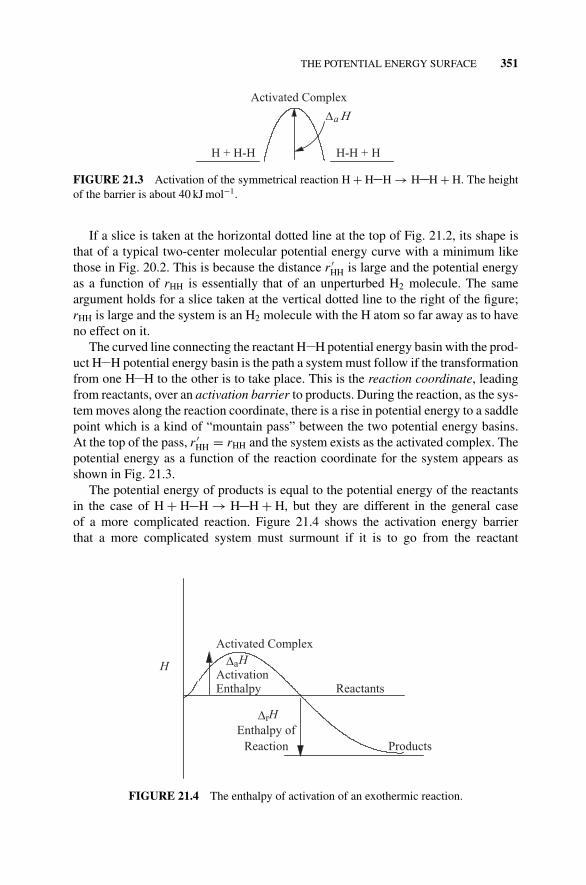
P1: OTA/XYZ P2: ABCc21 JWBS043-Rogers September 13, 2010 11:30 Printer Name: Yet to Come
THE POTENTIAL ENERGY SURFACE 351
H + H-H H-H + H
Activated Complex
a
FIGURE 21.3 Activation of the symmetrical reaction H + H H → H H + H. The heightof the barrier is about 40 kJ mol−1.
If a slice is taken at the horizontal dotted line at the top of Fig. 21.2, its shape isthat of a typical two-center molecular potential energy curve with a minimum likethose in Fig. 20.2. This is because the distance r ′
HH is large and the potential energyas a function of rHH is essentially that of an unperturbed H2 molecule. The sameargument holds for a slice taken at the vertical dotted line to the right of the figure;rHH is large and the system is an H2 molecule with the H atom so far away as to haveno effect on it.
The curved line connecting the reactant H H potential energy basin with the prod-uct H H potential energy basin is the path a system must follow if the transformationfrom one H H to the other is to take place. This is the reaction coordinate, leadingfrom reactants, over an activation barrier to products. During the reaction, as the sys-tem moves along the reaction coordinate, there is a rise in potential energy to a saddlepoint which is a kind of “mountain pass” between the two potential energy basins.At the top of the pass, r ′
HH = rHH and the system exists as the activated complex. Thepotential energy as a function of the reaction coordinate for the system appears asshown in Fig. 21.3.
The potential energy of products is equal to the potential energy of the reactantsin the case of H + H H → H H + H, but they are different in the general caseof a more complicated reaction. Figure 21.4 shows the activation energy barrierthat a more complicated system must surmount if it is to go from the reactant
Activated Complex
ActivationEnthalpy Reactants
Enthalpy of Reaction Products
H
rH
aH
FIGURE 21.4 The enthalpy of activation of an exothermic reaction.
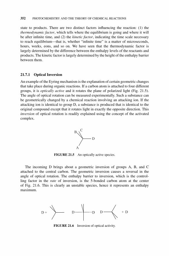
P1: OTA/XYZ P2: ABCc21 JWBS043-Rogers September 13, 2010 11:30 Printer Name: Yet to Come
352 PHOTOCHEMISTRY AND THE THEORY OF CHEMICAL REACTIONS
state to products. There are two distinct factors influencing the reaction: (1) thethermodynamic factor, which tells where the equilibrium is going and where it willbe after infinite time, and (2) the kinetic factor, indicating the time scale necessaryto reach equilibrium—that is, whether “infinite time” is a matter of microseconds,hours, weeks, eons, and so on. We have seen that the thermodynamic factor islargely determined by the difference between the enthalpy levels of the reactants andproducts. The kinetic factor is largely determined by the height of the enthalpy barrierbetween them.
21.7.1 Optical Inversion
An example of the Eyring mechanism is the explanation of certain geometric changesthat take place during organic reactions. If a carbon atom is attached to four differentgroups, it is optically active and it rotates the plane of polarized light (Fig. 21.5).The angle of optical rotation can be measured experimentally. Such a substance canbe geometrically changed by a chemical reaction involving an attacking ion. If theattacking ion is identical to group D, a substance is produced that is identical to theoriginal compound except that it rotates light in exactly the opposite direction. Thisinversion of optical rotation is readily explained using the concept of the activatedcomplex.
A
B C
D
FIGURE 21.5 An optically active species.
The incoming D brings about a geometric inversion of groups A, B, and Cattached to the central carbon. The geometric inversion causes a reversal in theangle of optical rotation. The enthalpy barrier to inversion, which is the control-ling factor in the rate of inversion, is the 5-bonded carbon atom at the centerof Fig. 21.6. This is clearly an unstable species, hence it represents an enthalpymaximum.
D + D D D + D
FIGURE 21.6 Inversion of optical activity.
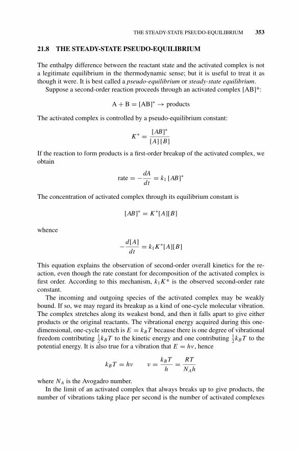
P1: OTA/XYZ P2: ABCc21 JWBS043-Rogers September 13, 2010 11:30 Printer Name: Yet to Come
THE STEADY-STATE PSEUDO-EQUILIBRIUM 353
21.8 THE STEADY-STATE PSEUDO-EQUILIBRIUM
The enthalpy difference between the reactant state and the activated complex is nota legitimate equilibrium in the thermodynamic sense; but it is useful to treat it asthough it were. It is best called a pseudo-equilibrium or steady-state equilibrium.
Suppose a second-order reaction proceeds through an activated complex [AB]*:
A + B = [AB]∗ → products
The activated complex is controlled by a pseudo-equilibrium constant:
K ∗ = [AB]∗
[A] [B]
If the reaction to form products is a first-order breakup of the activated complex, weobtain
rate = −dA
dt= k1 [AB]∗
The concentration of activated complex through its equilibrium constant is
[AB]∗ = K ∗[A][B]
whence
−d[A]
dt= k1 K ∗[A][B]
This equation explains the observation of second-order overall kinetics for the re-action, even though the rate constant for decomposition of the activated complex isfirst order. According to this mechanism, k1 K * is the observed second-order rateconstant.
The incoming and outgoing species of the activated complex may be weaklybound. If so, we may regard its breakup as a kind of one-cycle molecular vibration.The complex stretches along its weakest bond, and then it falls apart to give eitherproducts or the original reactants. The vibrational energy acquired during this one-dimensional, one-cycle stretch is E = kB T because there is one degree of vibrationalfreedom contributing 1
2 kB T to the kinetic energy and one contributing 12 kB T to the
potential energy. It is also true for a vibration that E = hv , hence
kB T = hv ν = kB T
h= RT
NAh
where NA is the Avogadro number.In the limit of an activated complex that always breaks up to give products, the
number of vibrations taking place per second is the number of activated complexes
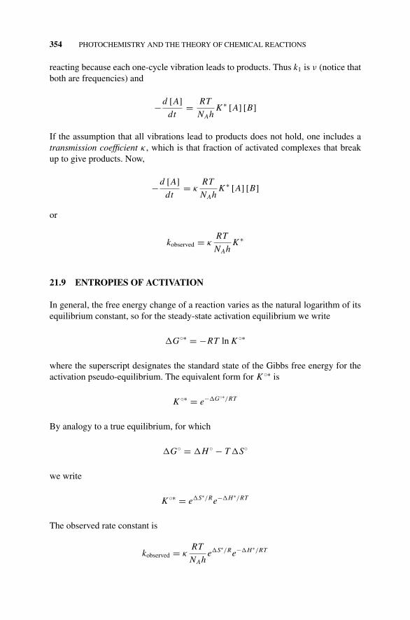
P1: OTA/XYZ P2: ABCc21 JWBS043-Rogers September 13, 2010 11:30 Printer Name: Yet to Come
354 PHOTOCHEMISTRY AND THE THEORY OF CHEMICAL REACTIONS
reacting because each one-cycle vibration leads to products. Thus k1 is ν (notice thatboth are frequencies) and
−d [A]
dt= RT
NAhK ∗ [A] [B]
If the assumption that all vibrations lead to products does not hold, one includes atransmission coefficient κ , which is that fraction of activated complexes that breakup to give products. Now,
−d [A]
dt= κ
RT
NAhK ∗ [A] [B]
or
kobserved = κRT
NAhK ∗
21.9 ENTROPIES OF ACTIVATION
In general, the free energy change of a reaction varies as the natural logarithm of itsequilibrium constant, so for the steady-state activation equilibrium we write
�G◦∗ = −RT ln K ◦∗
where the superscript designates the standard state of the Gibbs free energy for theactivation pseudo-equilibrium. The equivalent form for K ◦∗ is
K ◦∗ = e−�G◦∗/RT
By analogy to a true equilibrium, for which
�G◦ = �H ◦ − T �S◦
we write
K ◦∗ = e�S∗/Re−�H∗/RT
The observed rate constant is
kobserved = κRT
NAhe�S∗/Re−�H∗/RT

P1: OTA/XYZ P2: ABCc21 JWBS043-Rogers September 13, 2010 11:30 Printer Name: Yet to Come
PROBLEMS AND EXAMPLES 355
which can be compared with the Arrhenius equation
kobserved = se−�Ha/RT
Noting that �Ha in Arrhenius theory is the same thing as �H∗ in Eyring’s theory,the preexponential s must be
s = κRT
NAhe�S∗/R
This expression gives a preexponential that is a function of the temperature as con-trasted to Arrhenius’ conclusion that s is constant. Accurate measurements haveindeed shown the temperature dependence of the supposed constant s.
21.10 THE STRUCTURE OF THE ACTIVATED COMPLEX
If the activated complex has a “tight” structure, its formation implies a reductionof freedom in the system, therefore a negative entropy change �S. If the activatedcomplex has a loose structure by comparison to the reactants, �S is positive hencethe preexponential factor is large as well. For some reactions, e−�Ha/RT may beunfavorable but the reaction rate is appreciable because of a large preexponential.
The reactions
NO + O3 = NO2 + O2
and
CH3I + HI = CH4 + I2
have been shown to have second-order rate constants k = 6.3 × 10⁷√
T e−2300/RT
and k = 5.2 × 10¹⁰√
T e−33,000/RT , respectively. Analyzing these two results, weconclude that the first reaction has a low activation barrier relative to the second andit has a lower preexponential than the second reaction. The entropy of activation ismore negative for the nitric oxide oxidation than the iodine abstraction, suggestinga tightly bound structure for the first activated complex and a loose structure for thesecond activated complex.
PROBLEMS AND EXAMPLES
Example 21.1 A C C Bond Dissociation Enthalpy (BDE)
Find the enthalpy of dissociation (BDE) of the C C bond in ethane in the G3(MP2)model chemistry.
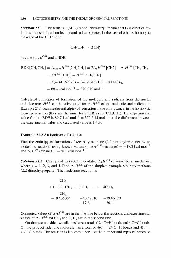
P1: OTA/XYZ P2: ABCc21 JWBS043-Rogers September 13, 2010 11:30 Printer Name: Yet to Come
356 PHOTOCHEMISTRY AND THE THEORY OF CHEMICAL REACTIONS
Solution 21.1 The term “G3(MP2) model chemistry” means that G3(MP2) calcu-lations are used for all molecular and radical species. In the case of ethane, homolyticcleavage of the C C bond
CH3CH3 → 2 CH•3
has a �dissoc H 298 and a BDE:
BDE [CH3CH3] = �dissoc H 298 [CH3CH3] = 2�f H 298[CH•
3
] − �f H 298 [CH3CH3]
= 2H 298[CH•
3
] − H 298 [CH3CH3]
= 2 (−39.752873) − (−79.646716) = 0.1410Eh
= 88.4 kcal mol−1 = 370.0 kJ mol−1
Calculated enthalpies of formation of the molecule and radicals from the nucleiand electrons H 298 can be substituted for �f H 298 of the molecule and radicals inExample 21.1 because the enthalpies of formation of the atoms cancel in the homolyticcleavage reaction (they are the same for 2 CH•
3 as for CH3CH3). The experimentalvalue for this BDE is 89.7 kcal mol−1 = 375.3 kJ mol−1, so the difference betweenthe experimental value and calculated value is 1.4%.
Example 21.2 An Isodesmic Reaction
Find the enthalpy of formation of tert-butylmethane (2,2-dimethylpropane) by anisodesmic reaction using known values of �f H 298(methane) = −17.8 kcal mol−1
and �f H 298(ethane) = −20.1 kcal mol−1.
Solution 21.2 Cheng and Li (2003) calculated �f H 298 of n-tert-butyl methanes,where n = 1, 2, 3, and 4. Find �f H 298 of the simplest example tert-butylmethane(2,2-dimethylpropane). The isodesmic reaction is
CH3|CH3−C−CH3 + 3CH4 −→ 4C2H6|
CH3
−197.35354 −40.42210 −79.65120−17.8 −20.1
Computed values of �f H 298 are in the first line below the reaction, and experimentalvalues of �f H 298 for CH4 and C2H6 are in the second line.
On the reactant side, two alkanes have a total of 24 C H bonds and 4 C C bonds.On the product side, one molecule has a total of 4(6) = 24 C H bonds and 4(1) =4 C C bonds. The reaction is isodesmic because the number and types of bonds on
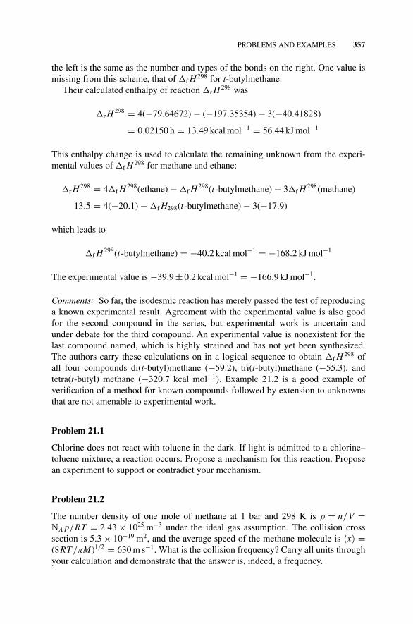
P1: OTA/XYZ P2: ABCc21 JWBS043-Rogers September 13, 2010 11:30 Printer Name: Yet to Come
PROBLEMS AND EXAMPLES 357
the left is the same as the number and types of the bonds on the right. One value ismissing from this scheme, that of �f H 298 for t-butylmethane.
Their calculated enthalpy of reaction �r H 298 was
�r H 298 = 4(−79.64672) − (−197.35354) − 3(−40.41828)
= 0.02150 h = 13.49 kcal mol−1 = 56.44 kJ mol−1
This enthalpy change is used to calculate the remaining unknown from the experi-mental values of �f H 298 for methane and ethane:
�r H 298 = 4�f H 298(ethane) − �f H 298(t-butylmethane) − 3�f H 298(methane)
13.5 = 4(−20.1) − �f H298(t-butylmethane) − 3(−17.9)
which leads to
�f H 298(t-butylmethane) = −40.2 kcal mol−1 = −168.2 kJ mol−1
The experimental value is −39.9 ± 0.2 kcal mol−1 = −166.9 kJ mol−1.
Comments: So far, the isodesmic reaction has merely passed the test of reproducinga known experimental result. Agreement with the experimental value is also goodfor the second compound in the series, but experimental work is uncertain andunder debate for the third compound. An experimental value is nonexistent for thelast compound named, which is highly strained and has not yet been synthesized.The authors carry these calculations on in a logical sequence to obtain �f H 298 ofall four compounds di(t-butyl)methane (−59.2), tri(t-butyl)methane (−55.3), andtetra(t-butyl) methane (−320.7 kcal mol−1). Example 21.2 is a good example ofverification of a method for known compounds followed by extension to unknownsthat are not amenable to experimental work.
Problem 21.1
Chlorine does not react with toluene in the dark. If light is admitted to a chlorine–toluene mixture, a reaction occurs. Propose a mechanism for this reaction. Proposean experiment to support or contradict your mechanism.
Problem 21.2
The number density of one mole of methane at 1 bar and 298 K is ρ = n/V =NA p/RT = 2.43 × 1025 m−3 under the ideal gas assumption. The collision crosssection is 5.3 × 10⁻¹⁹ m2, and the average speed of the methane molecule is 〈x〉 =(8RT /πM)1/2 = 630 m s−1. What is the collision frequency? Carry all units throughyour calculation and demonstrate that the answer is, indeed, a frequency.
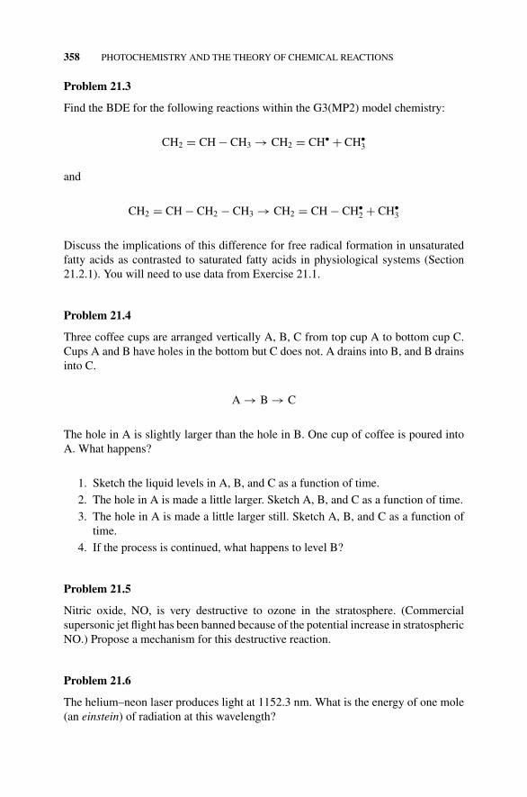
P1: OTA/XYZ P2: ABCc21 JWBS043-Rogers September 13, 2010 11:30 Printer Name: Yet to Come
358 PHOTOCHEMISTRY AND THE THEORY OF CHEMICAL REACTIONS
Problem 21.3
Find the BDE for the following reactions within the G3(MP2) model chemistry:
CH2 = CH − CH3 → CH2 = CH• + CH•3
and
CH2 = CH − CH2 − CH3 → CH2 = CH − CH•2 + CH•
3
Discuss the implications of this difference for free radical formation in unsaturatedfatty acids as contrasted to saturated fatty acids in physiological systems (Section21.2.1). You will need to use data from Exercise 21.1.
Problem 21.4
Three coffee cups are arranged vertically A, B, C from top cup A to bottom cup C.Cups A and B have holes in the bottom but C does not. A drains into B, and B drainsinto C.
A → B → C
The hole in A is slightly larger than the hole in B. One cup of coffee is poured intoA. What happens?
1. Sketch the liquid levels in A, B, and C as a function of time.
2. The hole in A is made a little larger. Sketch A, B, and C as a function of time.
3. The hole in A is made a little larger still. Sketch A, B, and C as a function oftime.
4. If the process is continued, what happens to level B?
Problem 21.5
Nitric oxide, NO, is very destructive to ozone in the stratosphere. (Commercialsupersonic jet flight has been banned because of the potential increase in stratosphericNO.) Propose a mechanism for this destructive reaction.
Problem 21.6
The helium–neon laser produces light at 1152.3 nm. What is the energy of one mole(an einstein) of radiation at this wavelength?

P1: OTA/XYZ P2: ABCc21 JWBS043-Rogers September 13, 2010 11:30 Printer Name: Yet to Come
PROBLEMS AND EXAMPLES 359
Problem 21.7
Irradiation of a gaseous sample of acetone(g) by light of 313 nm brings about pho-tochemical dissociation to give ethane(g) and CO(g). If, in an experimental run, thetotal radiant energy was 200 J and 9.00 × 10⁻⁵ moles of acetone dissociated, whatwas the quantum yield?
Problem 21.8
Part of chemical folklore is that heating a reaction by 10 degrees doubles the rate.If this is true, what is the activation energy for the temperature change from 298 to308 K? Is this rule generally true?

P1: OTA/XYZ P2: ABCc21 JWBS043-Rogers September 13, 2010 11:30 Printer Name: Yet to Come
P1: OTA/XYZ P2: ABCref JWBS043-Rogers September 15, 2010 1:42 Printer Name: Yet to Come
REFERENCES
Allinger, N. L. 2010. Molecular Structures, John Wiley & Sons, Hoboken NJ.
Allinger, N. L.; Chen, K.; Lii, J.-H. 1996. J. Comp. Chem. 17, 642–668.
Atkins, P. W. 1998. Physical Chemistry, 6th ed., Freeman, New York.
Atkins, P. W.; Friedman, R. S. 1997. Molecular Quantum Mechanics, 3rd ed., Oxford,New York.
Barrante, J. R. 1998. Applied Mathematics for Physical Chemistry, 2nd ed., Prentice-Hall,Englewood Cliffs, NJ.
Becke, A. D. 1933. J. Chem. Phys. 98, 1372–1377, 5648–5652.
Barrow, G. M. 1996. Physical Chemistry, 6th ed., WCB/McGraw-Hill, New York.
Bohr, N. 1913. Philos. Mag. 26, 1–25.
Born, M.; Heisenberg, W.; Jordan, P. 1926. Z. Phys. 35, 557–615.
Cheng, M. F.; Li, W.-K. 2003. J. Phys. Chem. A 107, 5492–5498.
Cohen, N.; Benson, S. W. 1993. Chem. Rev. 93, 2419–2438.
CRC Handbook of Chemistry and Physics, 2008–2009, 89th ed., Lide, D. R.; ed., CRC Press,Boca Raton, FL.
Curtiss, L. A., et al. 1999. J. Chem. Phys. 110, 4703–4709.
De Broglie, L. 1924. Thesis, Paris. 1926. Ann. Phys. 3, 22. See also Pauling, L.; Wilson,E. B. 1935. Introduction to Quantum Mechanics, McGraw-Hill, New York. Reprinted1963, Dover, New York.
Ebbing, D. D.; Gammon. S. D. 1999. General Chemistry, 6th ed., Houghton Mifflin, Boston.
Ege, S. N. 1994. Organic Chemistry; Structure and Reactivity, 3rd ed., D. C. Heath, Lexington,MA.
Concise Physical Chemistry, by Donald W. RogersCopyright C© 2011 John Wiley & Sons, Inc.
361
P1: OTA/XYZ P2: ABCref JWBS043-Rogers September 15, 2010 1:42 Printer Name: Yet to Come
362 REFERENCES
Eyring, H. 1935. J. Chem. Phys. 3, 107–115.
Fock, V. 1930. Z. Phys. 61, 126–148.
Gibson, D. G., et al. 2010. Science 329, 52–56.
Hammes, G. G., 2007. Physical Chemistry for the Biological Sciences, John Wiley & Sons,Hoboken, NJ.
Hartree, D. R. 1928. Proc. Cambridge Philos. Soc. 24, 89–111, 111–132.
Hehre, W. 2006. Computational Chemistry, in Engel T., Quantum Chemistry and Spectroscopy,Pearson-Benjamin Cummings, New York.
Hehre W. J., et al. 1970. J. Am. Chem. Soc. 92, 4766–4801.
Heisenberg, W. 1925. Z. Phys. 33, 879–893.
Heitler, W.; London, F. 1927. Z. Phys. 44, 455–472.
Henry, W. 1803. Philsophical Transactions of the Royal Society.
Houston, P. L. 2006. Chemical Kinetics and Reaction Dynamics, Dover Publications, Mineola,New York.
Irikura, K. K. Essential Statistical Thermodynamics in Computational Thermochemistry, inIrikura, K. K.; Furrip, D. J., eds. 1998. Computational Thermochemistry, American Chem-ical Society, Washington, D.C.
Kistiakowsky, G. B., et al. 1935. J Am. Chem. Soc. 57, 65–75.
Klotz, I. M.; Rosenberg, R. M. 2008. Chemical Thermodynamics. Basic Theory and Methods,7th ed., J. Wiley Interscience, New York.
Kondipudi, D.; Prigogine, I. 1998. Modern Thermodynamics: From Heat Engines to DissipativeStructures, John Wiley & Sons, New York.
Laidler, K. J.; Meiser, J. H. 1999. Physical Chemistry, 3rd ed., Houghton Mifflin, Boston.
Lee, C. et al. Phys. Rev., 37, 785–789.
Levine, I. N. 2000. Quantum Chemistry, 5th ed., Prentice-Hall, New York.
Levine, I. 2000. Physical Chemistry 6th ed. McGraw-Hill Inc., New York.
Lewis, G. N.; Randall, M., revised by Pitzer K. S.; Brewer, L. 1961. Thermodynamics,2nd ed., McGraw-Hill, New York.
Maczek, A. 1998. Statistical Thermodynamics, Oxford Science, New York.
McQuarrie, D. A. 1983. Quantum Chemistry, University Science Books, Mill Valley, CA.
McQuarrie, D. H.; Simon, J. D. 1997. Physical Chemistry: A Molecular Approach, UniversityScience Books, Sausalito, CA.
Metiu, H. 2006. Physical Chemistry, Taylor and Francis, New York.
Moeller C.; Plesset, M. S. 1934. Phys. Rev. 46, 618–622. See also Cramer, C. J. 2004. Compu-tational Chemistry 2nd ed., John Wiley & Sons, Hoboken NJ.
Nash, L. K. 2006. Elements of Statistical Thermodynamics, 2nd ed. Dover Publications,Mineola, New York.
Nevins, N.; Chen, K.; Allinger, N. L. 1996a. J. Comp. Chem. 17, 669–694.
Nevins, N.; Lii, J.-H.; Allinger, N. L. 1996b. J. Comp. Chem. 17, 695–729.
Pauling, L.; Wilson, E. B. 1935. Introduction to Quantum Mechanics, McGraw-Hill, NewYork. Reprinted 1963, Dover Publications, New York.
Petersson, G. A. 1998. Complete basis set thermochemistry and kinetics, in Irikura, K. K.;Furrip, D. J., eds., Computational Thermochemistry. American Chemical Society, Wash-ington, D.C.

P1: OTA/XYZ P2: ABCref JWBS043-Rogers September 15, 2010 1:42 Printer Name: Yet to Come
REFERENCES 363
Petersson et al. 1991. J. Chem. Phys., 94, 6081–6090, 6091–6101.
Pitzer K. S.; Brewer, L. Revision of Lewis, G. N.; Randall, M. 1961. Thermodynamics,2nd ed., McGraw-Hill, New York.
Planck, M. 1901. Ann. Phys. 4, 553–563; 717–727. See also Kuhn, T. S. 1978. Black BodyTheory and the Quantum Discontinuity 1894–1912, The University of Chicago Press,Chicago; and Oxford, New York.
Pople, J. A. 1999. Nobel lectures. Rev. Mod. Phys. 71, 1267–1274.
Rioux, F. 1987. Eur. J. Phys. 8, 297–299.
Rogers, D. W., et al. 2003. Org. Lett. 5, 2373–2375.
Rogers, D. W. 2005. Einstein’s Other Theory. The Planck-Bose-Einstein Theory of HeatCapacity. Princeton University Press, NJ.
Rogers, D. W.; Zavitsas, A. A.; Matsunaga, N. 2005. J. Phys. Chem. A 109, 9169–9173.
Rogers, D. W.; Matsunaga, N.; Zavitsas, A. A. 2006. J. Org. Chem. 71, 2214–2219.
Rogers, D. W.; Zavitsas, A. A.; Matsunaga, N., 2009. J. Phys. Chem. A, 113, 12049–12055.
Rosenberg, R. M.; Peticolas, W. L. 2004. J. Chem. Ed. 81, 1647–1652.
Schrodinger, E. 1925. Z. Phys. 33, 879.
Schrodinger, E. 1926. Ann. Phys. 79, 361, Ann. Phys. 79, 734.
Silbey, R. J. et al. 2005. Physical Chemistry 4th ed., John Wiley & Sons, Hoboken NJ.
Slater, J. C. 1930. Phys. Rev. 35, 210–211.
Steiner, E. 1996. The Chemistry Maths Book, Oxford Science Publications, NY.
Streitwieser Jr., A. 1961. Molecular Orbital Theory, John Wiley & Sons, Hoboken NJ.
Treptow, R. S. 2010. J. Chem. Ed. 87, 168–171.
Uhlenbeck G. E.; Goudsmit, S. 1925. Naturwissenschaften 13, 953–954.
Webbook.nist.gov
Zavitsas, A. A. 2001. J. Chem. Ed. 78, 417–419.
Zavitsas, A. A.; Rogers, D. W.; Matsunaga, N. 2008. J. Phys. Chem. A 112, 5734–5741.
Zewail, A. H. 1994. Femptochemistry: Ultrafast Dynamics of the Chemical Bond, Vols. 1and 2, World Scientific, Singapore.

P1: OTA/XYZ P2: ABCref JWBS043-Rogers September 15, 2010 1:42 Printer Name: Yet to Come
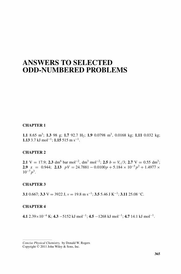
P1: OTA/XYZ P2: ABCans JWBS043-Rogers September 15, 2010 1:22 Printer Name: Yet to Come
ANSWERS TO SELECTEDODD-NUMBERED PROBLEMS
CHAPTER 1
1.1 8.65 m3; 1.3 98 g; 1.7 92.7 H2; 1.9 0.0798 m3, 0.0168 kg; 1.11 0.032 kg;1.13 3.7 kJ mol−1; 1.15 515 m s−1.
CHAPTER 2
2.1 V = 17.9; 2.3 dm6 bar mol−2, dm3 mol−2; 2.5 b = Vc/3; 2.7 V = 0.55 dm3;2.9 z = 0.944; 2.13 pV = 24.7881 − 0.0100p + 5.184 × 10⁻⁵ p2 + 1.4977 ×10⁻⁷ p3.
CHAPTER 3
3.1 0.667; 3.3 V = 3922 J, v = 19.8 m s−1; 3.5 5.46 J K−1; 3.11 25.08 ◦C.
CHAPTER 4
4.1 2.39×10⁻⁴ K; 4.3 −5152 kJ mol−1; 4.5 −1268 kJ mol−1; 4.7 14.1 kJ mol−1.
Concise Physical Chemistry, by Donald W. RogersCopyright C© 2011 John Wiley & Sons, Inc.
365
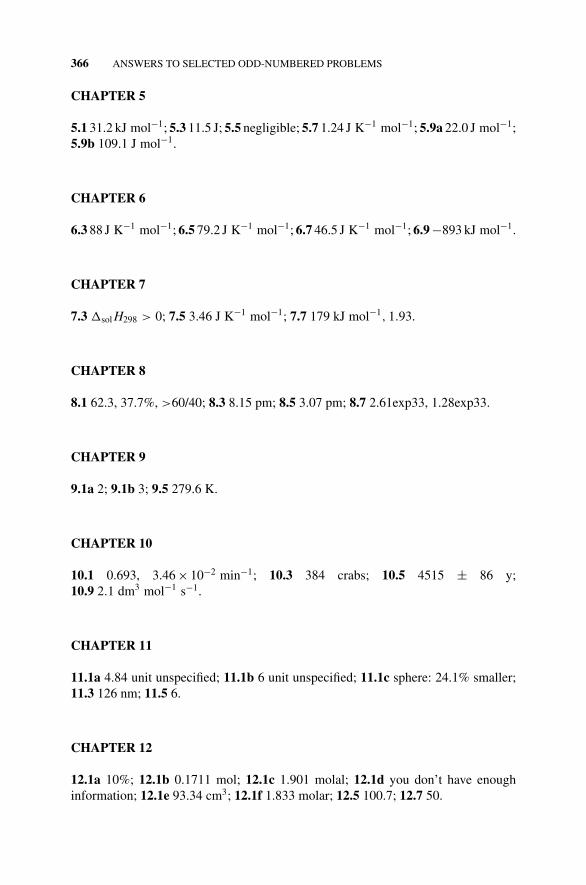
P1: OTA/XYZ P2: ABCans JWBS043-Rogers September 15, 2010 1:22 Printer Name: Yet to Come
366 ANSWERS TO SELECTED ODD-NUMBERED PROBLEMS
CHAPTER 5
5.1 31.2 kJ mol−1; 5.3 11.5 J; 5.5 negligible; 5.7 1.24 J K−1 mol−1; 5.9a 22.0 J mol−1;5.9b 109.1 J mol−1.
CHAPTER 6
6.3 88 J K−1 mol−1; 6.5 79.2 J K−1 mol−1; 6.7 46.5 J K−1 mol−1; 6.9 −893 kJ mol−1.
CHAPTER 7
7.3 �sol H298 > 0; 7.5 3.46 J K−1 mol−1; 7.7 179 kJ mol−1, 1.93.
CHAPTER 8
8.1 62.3, 37.7%, >60/40; 8.3 8.15 pm; 8.5 3.07 pm; 8.7 2.61exp33, 1.28exp33.
CHAPTER 9
9.1a 2; 9.1b 3; 9.5 279.6 K.
CHAPTER 10
10.1 0.693, 3.46 × 10⁻² min−1; 10.3 384 crabs; 10.5 4515 ± 86 y;10.9 2.1 dm3 mol−1 s−1.
CHAPTER 11
11.1a 4.84 unit unspecified; 11.1b 6 unit unspecified; 11.1c sphere: 24.1% smaller;11.3 126 nm; 11.5 6.
CHAPTER 12
12.1a 10%; 12.1b 0.1711 mol; 12.1c 1.901 molal; 12.1d you don’t have enoughinformation; 12.1e 93.34 cm3; 12.1f 1.833 molar; 12.5 100.7; 12.7 50.
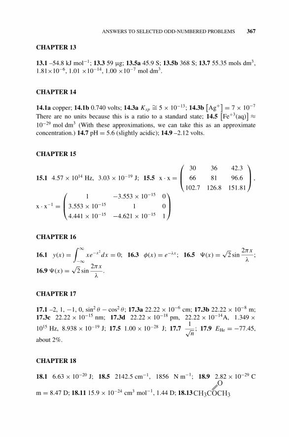
P1: OTA/XYZ P2: ABCans JWBS043-Rogers September 15, 2010 1:22 Printer Name: Yet to Come
ANSWERS TO SELECTED ODD-NUMBERED PROBLEMS 367
CHAPTER 13
13.1 –54.8 kJ mol−1; 13.3 59 µg; 13.5a 45.9 S; 13.5b 368 S; 13.7 55.35 mols dm3,1.81×10−6, 1.01 ×10⁻¹⁴, 1.00 ×10⁻⁷ mol dm3.
CHAPTER 14
14.1a copper; 14.1b 0.740 volts; 14.3a Ksp∼= 5 × 10⁻¹³; 14.3b
[Ag+] = 7 × 10⁻⁷
There are no units because this is a ratio to a standard state; 14.5[Fe+3(aq)
] ≈10−29 mol dm3 (With these approximations, we can take this as an approximateconcentration.) 14.7 pH = 5.6 (slightly acidic); 14.9 –2.12 volts.
CHAPTER 15
15.1 4.57 × 10¹⁴ Hz, 3.03 × 10⁻¹⁹ J; 15.5 x · x =
⎛⎜⎝
30 36 42.3
66 81 96.6
102.7 126.8 151.81
⎞⎟⎠ ,
x · x−1 =
⎛⎜⎝
1 −3.553 × 10⁻¹⁵ 0
3.553 × 10⁻¹⁵ 1 0
4.441 × 10⁻¹⁵ −4.621 × 10⁻¹⁵ 1
⎞⎟⎠
CHAPTER 16
16.1 y(x) =∫ ∞
−∞xe−x2
dx = 0; 16.3 φ(x) = e−λx ; 16.5 �(x) = √2 sin
2πx
λ;
16.9 �(x) = √2 sin
2πx
λ.
CHAPTER 17
17.1 –2, 1, −1, 0, sin2 θ − cos2 θ ; 17.3a 22.22 × 10⁻⁶ cm; 17.3b 22.22 × 10⁻⁸ m;17.3c 22.22 × 10⁻¹⁵ nm; 17.3d 22.22 × 10⁻¹⁸ pm, 22.22 × 10⁻¹⁴A, 1.349 ×10¹⁵ Hz, 8.938 × 10⁻¹⁹ J; 17.5 1.00 × 10⁻²⁸ J; 17.7
1√n
; 17.9 EHe = −77.45,
about 2%.
CHAPTER 18
18.1 6.63 × 10⁻²⁰ J; 18.5 2142.5 cm−1, 1856 N m−1; 18.9 2.82 × 10⁻²⁹ C
m = 8.47 D; 18.11 15.9 × 10⁻²⁴ cm3 mol−1, 1.44 D; 18.13
P1: OTA/XYZ P2: ABCans JWBS043-Rogers September 15, 2010 1:22 Printer Name: Yet to Come
368 ANSWERS TO SELECTED ODD-NUMBERED PROBLEMS
CHAPTER 19
19.1a −168 kJ mol−1; 19.1b −7 kJ mol−1; 19.3 105.1◦. The experimental valueis 104.5◦; 19.7 −31.7 kcal mol−1 = −132.7 kJ mol−1. The experimental value is−32.60 ± 0.05 kcal mol−1 = 136.4 ± 0.2 kJ mol−1.
CHAPTER 20
20.3 the degeneracy pattern is 1,2,1,2, unlike the 1,2,2,1 pattern in the more commonHuckel model; 20.7a UHF=−2.8874388; 20.7b UHF=−4.8708157; 20.7c Themolecule does not exist; 20.7d The molecule is lower in energy than its atoms by30.3 kcal mol−1 = 127 kJ mol−1. LiH exists and is used in organic chemistry as areducing agent.
CHAPTER 21
21.1 search for PhCH2CH2Ph in the product mixture; 21.3 100.2 kcal mol−1 and74.2 kcal mol−1; 21.7 0.17.
P1: OSOind JWBS043-Rogers September 24, 2010 12:57 Printer Name: Yet to Come
INDEX
1s STO and a Gaussian approximation,324
6-31G basis functions, 332
Ab Initio methods, 324Absorption wavelengths, 293
of conjugated polyalkenes, 293Acetic acid, 69Acetone, 196, 200Acetonitrile, 159Acidity constant, 209, 215Activated complex, 350, 355
enthalpy level diagram, 157structure, 355
Activation, 351activation barrier, 156, 157, 351
Activation energy, 344Activity, 97, 186
activity coefficient, 98, 186Additive extrapolations, 339
the G3(MP2) scripted method,339
Additive methods, 305Adenosine 5′-triphosphate ATP, 105Adiabatic work, 50
ADP, 107Ag ions, 212, 216–217Alkane conformers, 308Allinger MM method, 308Allinger, 64Ammonia, 82, 195, 201AMP, 107Amperostat, 215–216Amplitude function, 238, 249Anode, 223Antioxidants, 347Antisymmetric wave functions, 239Antisymmetrized orbitals, 240Arclength, 40Arrhenius law, 158, 349Atomic units, 243ATP, 103–104, 107Aufbau principle, 280Autooxidation, 346Avogadro, 3Azeotrope, 138
Bar (unit), 13BASIC, 83Basis function, 245, 320
Concise Physical Chemistry, by Donald W. RogersCopyright C© 2011 John Wiley & Sons, Inc.
369
P1: OSOind JWBS043-Rogers September 24, 2010 12:57 Printer Name: Yet to Come
370 INDEX
Battery, 221Benzene, 342Benzoic acid, 68Bimembrane, 167Bimolecularity, 155Binary solutions, 184Body-centered cubic cell, 180Bohr, 236, 264Boiling point elevation, 188Boltzmann 101, 108Boltzmann constant, 9Boltzmann distribution of molecular speeds,
158Bond additivity, 306Bond breaking, 350Bond dissociation energies (BDE), 348,
355, 358Bond energy, 65Bond enthalpies, 306Bond length, 292, 299Bond making, 350Bond moments, 296
dichloroethene isomers, 296Bond strength, 292, 299Born probability postulate, 252Born, 237Born-Haber cycle, 178–179Bosons and Fermions, 278Boyle, 1Bragg’s law, 173Bravais crystal systems, 176Bravais lattices, 176Breaking degeneracy, 259
Cadmium half-cell, 232Calculated ionization potentials,
281Calomel electrode, 229Calorie, 54Calorimeter, 104Calorimetry, 56Capacitance, 294Capillary rise, 167Carbon dioxide, 34, 86
free energy of formation, 87Carbon disulfide, 91, 92Carnot, 71Carnot’s engine, 72Cartesian space, 330
Cathode, 217, 223Cell diagrams, 223Cell reaction, 223Central field approximation, 239Cerium, 234Chain reaction, 153, 345–346
initiation, 346propagation, 346termination, 346
Charge distribution, 241Charles, 1Chemical kinetics, 144Chemical potential, 87
nonideal systems, 100, 102pressure dependence, 87temperature dependence, 88–89
Chemical reactions, 78, 79Chloroform, 200Clapeyron equation, 128Classical harmonic oscillator, 288Classical molecular modeling, 305Clausius, 71Clausius–Clapeyron equation, 128Close packing, 171Closed system, 41Coexistance curve, 127Colligative properties, 187, 194Collision theory, 158Combined gas law, 2, 12Combined or scripted methods, 338Combining enthalpy and entropy, 84Combustion of C(gr) and CO(g), 59Combustion, 92
free energy of, 92of methane, 92
Components, 124Components, phases, and degrees of
freedom, 124Compound phase diagrams, 137Compressibility factor, 20, 21, 28
calculated from the van der Waalsconstants, 28
Computational chemical script, 338Computational geometries, 177Computational kinetics, 159Computational statistical thermodynamics,
119GAUSSIAN 03 C©, 119
Computational thermochemistry, 100
P1: OSOind JWBS043-Rogers September 24, 2010 12:57 Printer Name: Yet to Come
INDEX 371
Computed partition functions, 120for molecular and atomic sodium, 120
Computer files, 273Concentration cells, 225Concentration units, 184Conductance cell, 206Conductance, 205, 211Conductivity, 203, 205Conservation laws, 35
exact differentials, 35Conservtive systems, 238Contracted Gaussian orbitals CTGO, 328Conversion of a Liquid to Its Vapor Without
Boiling, 25Copper electrode, 221Correlation energy, 337Corresponding states, 23, 27Coulomb (unit), 224Coulombs, 212Coulometry, 203Covalent bond radii, 176Critical density, 26Critical point, 25, 127Critical temperature, 24Cross term, 310Crystal forces in MM, 312Crystals, 170CTGO, 328Cubic (crystal) cell, 175Cubic equation, 28, 29Cubic real gas behavior, 34Curve-fitting software, 21
Dalton’s Law, 5Daniell cell, 220de Broglie, 235Debye-Huckel law, 213Degeneracy, 257
and equilibrium, 109Degenerate two-level equilibrium, 110Degree of dissociation, 208Degree of ionization, 208Degrees of freedom, 4, 124Density functional theory (DFT), 338Density ρ curves, 26
for liquid and gaseous oxygen, 26Dependent variables, 4Detailed balance, 152Determinantal wave functions, 240
Deviations from Raoult’s law, 185Dewar, 323Diatomic molecules, 290Dielectric constant, 294Dielectric, 294Diethyl ether, 196Different paths of transformations, 38Differential scanning calorimetry, 66Digression on “Space”, 9Dipole moments, 294, 301, 303Dipole, 294Discontinuous energy levels, 8Disorder, 74, 109, 183Distortion polarization, 295Distribution, 110DSC, 66
Early atomic theory, 235Early quantum theory, 236Ebullioscopic constant, 190Effective molecular weight (molar mass), 28Effective nuclear charge, 240Effective quantum number, 282Egyptian tomb, 163Eigenfunction postulate, 252Eigenvalues and eigenvectors, 250Einstein, 247Einstein’s law, 344Electrical potential, 203, 204Electrical work, 224Electrochemical cells, 220Electrochemical potential, 221Electrolyte, 203Electromagnetic spectrum, 235Electron spin resonance, 299Electronic promotion in alkenes, 293Electronic spectra, 292Empirical equations, 18Empirical gas laws, 1Energy and enthalpy, 44Energy equations, 308, 309Energy of formation, 57
indirect, 59Engine, 72Ensemble, 6, 7Enthalpies of formation of n-alkanes, 306Enthalpies of reaction, 60Enthalpy level diagram for an activated
complex, 157
P1: OSOind JWBS043-Rogers September 24, 2010 12:57 Printer Name: Yet to Come
372 INDEX
Enthalpy of activation, 351Enthalpy of formation, 57, 64
from classical mechanics, 64indirect, 59of hydrogenation, 61, 65–66
Enthalpy of fusion, 92, 200Enthalpy of vaporization, 129Enthalpy, 305Entropy, 71, 99, 113
and probability, 113and the second Law, 71from the van’t Hoff equation, 99
Entropy changes, 74chemical reactions, 78expansion, 75heat transfer, 77heating and expansion, 75heating, 74mixing, 77of transition, 75
Entropy of activation, 354Entropy, enthalpy, and Gibbs free energy
changes for mixing, 183Equations of state, 4Equilibrium, 93, 94, 108
and free energy, 99Equilibrium constant Keq , 73, 97
as a quotient of quotients, 88statistical approach, 117
sodium vapor, 117variation with temperature, 97
Equilibrium, 108Equilibrium, 94, 108
general formulation, 94Euler’s reciprocity relationship, 36,
76Eutectic mixture, 137Exact differentials, 36Excluded volume, 29Expectation value, 17Experimental determination of molecular
structure, 287Experimental determination of the rate
equation, 154Extensive variable, 6Extent of reaction, 96Extrapolation to E◦, 226, 227Eyring reaction path, 350Eyring theory of reaction rates, 349
Failure of perpetual motion, 39Faraday (unit), 211Faraday, 205Faraday’s laws, 211Favorable and unfavorable orbital overlap,
263First law of thermodynamics, 35–36First-order radioactive decay, 146First-order rate laws, 144–145Flash photolysis, 154Fluid, 25Fluorescence, 160–161, 345
mechanism of, 346Force constants and parameters, 308Force fields, 308, 310Frankenstein, 220Free electron model, 292Free energies of formation, 85Free energy and equilibrium, 102
in biochemical systems, 102Free energy, 87
of reaction, 87of formation, 90of methane, 90
Free solvent, 194Freezing point of water, 195Fugacity, 97
coefficient, 98Fundamental thermodynamic identities,
86Further basis set improvements, 336
G3(MP2), 338Gain medium, 348Galvani, 220GAMESS, 330, 340
calculation of methane, 340control lines, 341file for the hydrogen molecule, 330
Gas constant, 13Gaussian approximation, 272Gaussian basis set, 324Gaussian distribution, 7
in hyperspace, 10Gaussian distribution, 7Gaussian gen input, 273
for the hydrogen atom, 273energies, 273
GAUSSIAN C© input for hydrogen, 330
P1: OSOind JWBS043-Rogers September 24, 2010 12:57 Printer Name: Yet to Come
INDEX 373
Gaussian probability density distributions,10
Gaussian, 69GAUSSIAN C©, 69, 244
HF calculation of E , 273Gibbs chemical potential, 133, 192Gibbs free energy, 84, 112
and the partition function, 112of water, 126
Gibbs thermodynamic function, 76Gibbs–Helmholtz equation, 89Glass electrode, 230Glucose, 69Gordon, 323Graham’s Law of effusion, 6
molecular weight (molar mass)determination, 6
Group additivity, 62, 306hydrogen atom counting, 63
n-octane, 69GUI, 310
Half cells, 221Half-cell potentials, 222Half-time, 146Hamiltonian operator, 237, 251Harmonic oscillator, 287Hartree (unit), 272Hartree and Fock, 239Hartree equations, 242Hartree independent electron method, 240Hartree product, 263Hartree-Fock limit, 336Heat capacities and γ for selected real
gases, 48Heat capacity, 44, 48, 70
as a function of temperature, 50, 168of an ideal gas, 48
Heat capacity of liquids and solids, 168Heat death, 73Heat transfer, 77Heisenberg, 237Heitler and London, 238, 239Helium, 81, 243, 274Hemolytic cleavage, 348Henry’s law, 186Hermitian operators, 269Hess’s law, 61Heteroatoms: oxygen, 332
Hexa-1,3,5,-triene, 81Hey, Let’s Make a Perpetual Motion
Machine!, 38HF, 329Higher molecular orbital calculations, 322Hittorf cell, 211, 216HOMO, 285, 292Hooke’s law, 289Hooke’s potential well, 289Huckel, 271Hydrogen atom, 244, 258, 325Hydrogen emission spectrum, 236Hydrogen half-cell, 222Hydrogen molecule ion, 319
bonding and antibonding orbitals, 321,322
Hydrogen molecule, 329Hydrogen spectrum, 235Hydrogen-like atoms, 260
for an electron in the 3s orbital, 262higher exact solutions, 260radial probability density, 262roots of the radial 3s wave functions, 261the first six wave functions for hydrogen,
261the first three s wave functions for
hydrogen (simplified form), 261Hyper space, 3-, 4-, etc., 10
Ideal gas laws, 1Ideal solutions, 182Independent variables, 4, 125–126
coexistence curves, 125Influence of temperature on rate, 156Intensive variable, 6Intermolecular attraction at an air–water
interface, 166Internal and Cartesian coordinates, 334Interplanar (crystal) distances, 173Invasive crabs, 163Inversion of optical activity, 352Inversion temperature as a function of
pressure, 47Iodine vapor, 122, 123Ion activities, 213Ion mobilities, 209, 210, 211Ion speed, 210Ionic character, 297Ionic strength, 214
P1: OSOind JWBS043-Rogers September 24, 2010 12:57 Printer Name: Yet to Come
374 INDEX
Ionization potential IP, 274of helium, 284
Ion-permeable membrane, 204Irreversible change, 72Isobar, 26Isodesmic reactions, 349, 356Isolated system, 41Isotherm, 24
of a van der Waals gas, 24Iterative procedure, 241
Joule and Joule–Thomson experiments, 46Joule (unit), 42Joule, 46, 50
KCl, 62Kinetic energy, 7Kohlrausch’s law, 206
L-(dihydroxyphenyl)alanine, 218Laplace transforms, 149Lasers, 348Lattice energies, 177Law of corresponding states, another view,
27LCAO, 320L-Dopa, 218Le Chatelier’s principle, 99Lead, 83Length of an Arc, 40Limiting law, 214Line integrals, 39, 52–53Line spectrum, 235, 246Linear and angular momentum vectors, 283Linear combination, 270Linear combinations of atomic orbitals
LCAO, 322Lipid peroxidation, 346Liquids and solids, 165Liquid–vapor coexistence curve, 127Logarithmic decay of a radioactive element,
147LUMO, 285, 292
Magnetic resonance imaging (MRI), 299Making ATP, the cell’s power supply, 103Many-electron atomic systems, 263Mathcad C©, 52, 246Maxwell, 108
Maxwell-Boltzmann distribution, 7, 8, 13Mean activity coefficient of HCl, 232Mean ionic activity coefficients, 229Membrane potential, 203Methane, 331Methanol, 332
finding the enthalpy of formation,334–336
Methyl isocyanide, 159Microstates, 112Microwave spectroscopy, 292Mixing, 77MKS system, 2, 213MM series, 309
input file for water, 314thermodynamic properties, 311
MM4, 315geometry output for water, 315input geometry for methane, 316output geometry for methane, 316
Mobility, 211Models, 307Moeller-Plesset energies, 337Molality, 184, 197, 198Molar conductivity, 206
at infinite dilution, 207Molar heat capacities, 48Molar mass of a nonideal gas, 28Molar volume, 16, 33, 129Molarity, 198Mole fraction, 6, 184Molecular enthalpies of formation, 58Molecular mechanics, 309Molecular modeling, 310Molecular orbitals, 328Molecular quantum chemistry, 238Molecular variational method, 318Molecular velocities, 12Molecular weight (molar mass)
determination, 6Moles, 3Momentum, 15Moving boundary method, 210
NaCl conductivity, 219Naphthalene, 68NDDO and related approximations, 323Nernst equation, 224Newton’s second law, 14
P1: OSOind JWBS043-Rogers September 24, 2010 12:57 Printer Name: Yet to Come
INDEX 375
Nitric oxide, 358Nitrogen, 21, 222Nitrogen dioxide, 148Nitrogen tetroxide, 105NMR spectrum of ethanol, 299Nodes, 254
three wave functions, 254Born probability densities, 255
Nonideal binary solutions, 131Nonideal systems, chemical potential, 100Nonvolatile solute, 189Normalization, 257NSTP new standard temperature and
pressure, 16Nuclear magnetic resonance (NMR), 297,
304
Occupation number, 11Open system, 41Operator, 237Optical activity, 352Optical inversion, 352Optimizing the Gaussian function, 272Orbitals, 257Order and molecularity, 155Orientation polarization, 295Orthogonality, 262, 264
and overlap, 262Osmotic presure, 191, 192, 202Oxygen bomb calorimetry, 68Ozone depletion, 347Ozone hole, 156, 347Ozone, 155
Packing fraction, 174Parabola, 52Parabolic potential well, 290
of the harmonic oscillator, 290Parallel plate capacitor, 294Parametric curve fit, 19Partial GAUSSIAN G3(MP2) output, 339Partial ionization, 208Partial MM4 enthalpy output for ethane,
311Partial molar thermodynamic functions, 133
the general case, 133Partial molar volume, 129
as a slope of V vs n, 131the general case, 132
Partial pressure, 5, 6, 186, 195Particle in a cubic box, 255
the first excited state, 257Particle in a one-dimensional box, 253
energy, 265fundamentals and overtones, 254
Partition function, 10, 108, 111, 114, 118for different modes of motion, 116Gibbs free energy, 112rotational, 116vibrational, 115
Path independence, 38Path, 38Pauling, 239Perturbation, 337pH meter, 226Phase change, 84
water, 84Phase diagram, 127
water, 128Phase plane, 127Phase rule, 124Phases, 124Phosphorescence, 345
mechanism of, 346Photochemistry, 344Photoinduction, 345Physical equilibrium, 126Pitzer, 92Polar molecule, 297Polarizability, 295, 303Polarized basis functions, 332Pople, 323Population inversion, 348Population, 8Post-Hartree–Fock calculations, 336Potential drop, 204Potential energy surface, 350Potential enrgy, 42Pressure fraction, 5Primitives, 326Principle of detailed balance, 152Priogine, 42Probability “shells”, 258Probability, 12, 113
entropy and, 113Probability density, 8, 12, 241Probability factor, 159Pythagoras, 40

P1: OSOind JWBS043-Rogers September 24, 2010 12:57 Printer Name: Yet to Come
376 INDEX
QCISDT, 337Quadratic least squares, 21, 22Quadratic real gas behavior, 32Quantum mechanical systems, 251Quantum molecular modeling, 318Quantum numbers, 249, 277Quantum rigid rotor, 290
energy levels, 291Quantum yields, 345
experimental quantum yields, 345
Radial equation, 258Radial node of the 2p atomic orbital,
262Radiative decay, 161Radioactive decay, 144Raoult’s law, 183Rate controlling step, 155Ratio γ , 50–51, 55Reaction coordinate, 73, 351Reaction diagram, 88Reaction mechanisms, 154Reaction order, 149Reaction molecularity, 155Real gases, 18, 30Real solutions, 185Reciprocity relationship, 36Redox, 234Reduced variables, 27Reduction potentials, 223Reference states, 307Regression wizard, 31Reservoir, 72Resistivity, 205Resonance frequency, 291Reversible expansion, 43
of an ideal gas, 43Reversible processes, 42
path independence, 42Reversible reactions, 151RHF, 329Roothaan, 322Rotational symmetry, 171Route section, 329
Salt bridge, 223Saturated calomel electrode SCE, 229,
233Scalar, 251SCF Energies of atoms and ions, 281
SCF variational ionization potential forhelium, 275
Schrodinger equation, 64, 250GAMESS, 64Schrodinger, 237Second law of thermodynamics, 39Second virial coefficient, 22
as a function of temperature, 22Second-order reactions, 147–148Secular determinant, 268, 270Self consistent field (SCF), 243, 275,
277Semiempirical equation, 19Semiempirical methods, 323Semipermiable membrane, 191Separable equations, 256Sequential reactions, 150Shell structure, 331Shelley, 220Shielding constant, 280Shielding, 240Silver, standard entropy, 80, 81Silver–Silver chloride electrode, 227, 231,
234Sin(x), sin(2x), and sin(3x) [0, π ], 249Single-component phase diagram, 128Slater determinants, 279, 286Slater orbital, 276Slater, 282Slater’s rules, 282Slater-type orbitals (STO), 279, 282
oxygen, 284nitrogen, 285
Sodium vapor, 117Software, curve fitting, 21Solubility product constant, 228Solubility product, 228, 231Solute, 184Solution chemistry, 182Solvent, 184Space, 9
hyperspace, 3-, 4-, etc., 10spherical velocity space, 12velocity space, 12
Speed, 7Spherical polar coordinates, 259Spin, 278Spin–orbit coupling, 283Spin–spin coupling, 298Split valence basis sets, 331
P1: OSOind JWBS043-Rogers September 24, 2010 12:57 Printer Name: Yet to Come
INDEX 377
Spontaneous processes, 77chemical reactions, 78expansion, 75heating and expansion, 75heating, 74mixing, 77
Stability products, 228Standard hydrogen electrode SHE, 233Standard state, 103Standard states, 58State function, 237State functions (variables), 41, 45State of a System, 19State vector, 241State, 19Statistical approach to thermodynamics,
108Statistical thermodynamic functions
(Irikura, 1998), 114Statistical thermodynamic functions,
113Statistical thermodynamics, 108Steady-state approximation, 153Steady-state equilibrium, 353Stewart, 323STO-2G of hydrogen, 325
basis set, 325, 326STO-3G calculations on methanol, 333Stoichiometric coefficient, 96Stored parameters, 328
STO-2G basis for the 1s orbital ofhydrogen, 326–328
Strainless molecule, 307Stretching a two-dimensional membrane,
166Strong electrolytes, 208Structure, 307Subcritical fluids, 25Sucrose, 199Sulfur dioxide, 82Sum-over-states, 10Supercritical fluid, 25Surface tension, 165Surroundings, 41Symmetry, 340System, 19, 41
Temperature dependence of the Gibbs freeenergy, 88
Ternary phase diagrams, 138
Thermal protein denaturation, 67Thermal reaction, 67Thermal wavelength, 118, 120, 123
electronic, 116dissociation, 117translational, 116, 118
Thermochemical cycle, 60Thermochemistry, 56Thermodynamic cycles, 37Thermodynamic functions, 37, 41Thermodynamic property, 41Thermodynamic states and systems, 41Thermodynamics of simple systems, 35
the first law, 35Third law, 78Tie line, 137, 139Time’s arrow, 73Tocopherols, 347Total volume of an ideal binary solution,
130Transition states, 313Transition, 42Translational levels, 119Translational motion, 118
quantum number, 118thermal wavelength, 118
Transport number, 209, 211Triple point, 127
benzene, 143Trouton’s rule, 91Two-component phase diagrams, 134
Type 1, 135Type II, 136Type III, 137
Two-level equilibrium, 109, 111
UHF, 329Uncertainty principle, 238Unit cell, 174, 180Units, 2Universal gas constant, 13, 17Universe, 41, 73
Valence bond theory, 239van der Waals equation, 18van’t Hoff equation, 98Vapor pressure, 184, 187, 196
depression, 190Raoult’s law, 184
P1: OSOind JWBS043-Rogers September 24, 2010 12:57 Printer Name: Yet to Come
378 INDEX
Variation of enthalpy of formation with T ,65
Variation of the equilibrium constant withtemperature, 97
Variational method, 243, 267Variational treatment of the hydrogen atom,
271the energy spectrum, 271
Vector space, 268, 320Vector, 241Velocities of ideal gas particles, 8Velocity space, 11, 12Vibration-rotation band, 300, 302Vibration–rotation spectrum of CO, 302Virial equation, 19Virtual orbitals, 337Viscosity of liquids, 169
laminar flow, 169Poiseulle equation, 170viscosity coefficient, 170viscous drag, 169
Visualization, 310the ethane molecule via PCModel 8.0 C©,
310Vitamin E, 347Volta, 220Voltage, 203, 221Volume behavior of a nonideal binary
solution, 131Volume increase (or decrease) upon adding
solute, 130
Water, 84, 125, 128dissociation constant, 125enthalpy of vaporization, 139–140phase diagram, 128
Wave equations, 249two dimensions, 250three dimensions, 250
Wave function vector, 251Wave mechanics of simple systems, 248Wave motion, 248
amplitude, 249fundamental, 248overtone, 248
Weak electrolytes, 207, 208Work, 43
adiabatic, 50
x-Component, 13X-ray crystallography, 172X-ray diffraction, 173x-Space, 7
Z = f (p) Curve, 23for the same gas at two different
temperatures, 23for two different gases, 23
Zero point energy, 289Zinc electrode, 221z-Matrix format, 328, 329z-Matrix input file for methane, 340


