166


Concrete CausationAbout the Structures of Causal Knowledge
Inaugural-Dissertation zur Erlangungdes Doktorgrades der Philosophie an derLudwig-Maximilians-Universität München
vorgelegt von
Roland Poellinger, Münchenhttp://logic.rforge.com
Referent: Prof. Dr. Godehard Link(Lehrstuhl für Philosophie, Logik undWissenschaftstheorie, LMU München)
Korreferent: Prof. Dr. Thomas Augustin(Institut für Statistik, LMU München)
Tag der mündlichen Prüfung: 13.02.2012


I would like to thank the Alexander von Hum-boldt Foundation, which partially supportedmy work through funding the Munich Cen-ter for Mathematical Philosophy (MCMP) atLMU Munich. I am especially thankful to theLMU working group MindMapsCause, thathas shaped many of my thoughts in valuablediscussions.

Title image: tommy leong/Fotolia.com, R. Poellinger

Contents
1 Reasoning about causation 11.1 Causal powers . . . . . . . . . . . . . . . . . . . . . . . . . 21.2 Causal processes . . . . . . . . . . . . . . . . . . . . . . . 4
1.3 Natural experiments . . . . . . . . . . . . . . . . . . . . . 61.4 Logical reconstruction . . . . . . . . . . . . . . . . . . . . 7
1.5 Correlation and probabilistic causation . . . . . . . . . . . 101.6 Counterfactual analysis . . . . . . . . . . . . . . . . . . . 14
1.7 Ranking theory . . . . . . . . . . . . . . . . . . . . . . . . 191.8 Agency, manipulation, intervention . . . . . . . . . . . . . 22
1.9 Decisions to take . . . . . . . . . . . . . . . . . . . . . . . 28
2 Causation and causality: From Lewis to Pearl 332.1 What is a theory of causation about? . . . . . . . . . . . . 33
2.2 Hume’s counterfactual dictum . . . . . . . . . . . . . . . . 342.3 A possible worlds semantics with similarity . . . . . . . . 36
2.4 From counterfactual dependence to veritable causes . . . . 402.5 Pearl’s reply to Hume . . . . . . . . . . . . . . . . . . . 42
2.6 Pearl’s agenda . . . . . . . . . . . . . . . . . . . . . . . . 432.7 From modeling to model . . . . . . . . . . . . . . . . . . . 54
2.8 Triggering causes, bringing about effects . . . . . . . . . . 582.9 Computing observational data for causal inference . . . . 62
2.10 About the identifiability of effects in causal models . . . . 722.11 Singular causation and the actual cause . . . . . . . . . . 78
3 Causality as epistemic principle ofknowledge organization 85
3.1 The total system and the modality of interventions . . . . 863.2 Subnets for epistemic subjects . . . . . . . . . . . . . . . . 883.3 Organizing Data in causal knowledge patterns . . . . . . . 91
3.4 Causal knowledge patterns: design and manipulation . . . 953.5 Reviewing the framework . . . . . . . . . . . . . . . . . . 113

viii Contents
4 Modeling with causal knowledge patterns 1154.1 Causal decision theory, or: Of prisoners and predictors . . 1154.2 Meaningful isomorphisms . . . . . . . . . . . . . . . . . . 1304.3 Epistemic contours and the Markov assumption, revisited 134
A Random variables (stochastic variables) 137
B Technicalities: Implications of d-separation 141
References 151
Register of names 157
Chapter 1
Reasoning about causation
Felix qui potuit rerumcognoscere causas
Vergil, Georgica (II, 490)
Philosophers have been thinking systematically about cause and ef-fect since the very beginnings of philosophy as a discipline. Availingitself of mathematical methods and formal semantics in the last century,epistemology at once had the means to shape prevailing problems in sym-bolic form, express its achievements with scientific rigor, and sort issueswithin formal theories from questions about intuitions and basal pre-misses. David Lewis was among the first ones to utilize symbolic toolsand approach causality within a framework of formal semantics.1 AfterBertrand Russell had famously and brusquely turned his back on anyfurther pursuit of establishing criteria for causal analysis in his treatiseOn the Notion of Cause (1913), David Lewis re-thought the words of anearlier mind: In 1740 David Hume had listed causation among one of theprinciples that are “to us the cement of the universe” and thus “of vastconsequence [. . . ] in the science of human nature”.2 Hume gives varioushints about what his account of causation might be – one way of read-ing suggests that he argues for an innate human causal sense by whichwe discover the relation of causation in our surroundings.3 AlthoughHume is later sharply criticized for this empiricist account by ImmanuelKant, who in turn claims that causal principles are of synthetic a priori
1Cf. especially [Lewis 1973a].2These statements are from An Abstract of a “Treatise of Human Nature”.3Cf. [Garrett 2009].

2 Reasoning about causation
nature,4 David Lewis refers back to one specific counterfactual explica-tion of the semantics of causal statements in Hume’s writings, moreoverbases his thoughts on Humean supervenience, and unfolds a detailedmethod for causal analysis in the framework of his possible worlds se-mantics. Approaching the field from a computer science perspective inthe 1980s, Judea Pearl introduces networks of belief propagation asthe basis for Bayesian inference engines in an AI engineering context.5
His interventionist account of causation, most elaborately presented inhis book Causality (2000/2009), draws on structural transformations offormal causal models for the identification of cause-effect relations. Asa defendant of a thicker concept of causation, Nancy Cartwright de-cisively rejects Pearl’s thin, formal approach and makes a case for afamily-like understanding of causal concepts.
In the following chapters the line of thought from Lewis to Pearl
shall be traced, partly by examining their replies to one another, beforeI want to make the attempt to locate causation and causality in theontological landscape and try to pave the way for an epistemic under-standing of the relation of causation, finally applying this conception toexamples from recent and older philosophical literature. An overviewon ways of implementation and applications of the suggested methodswill conclude this text. Before getting into technical details, a short listof important approaches towards the analysis of causal concepts (andtheir most prominent advocates) shall be given – especially as a point ofreference and distinction for what follows. What suggestions have fueledthe philosophical discussion?
1.1 Causal powers
One metaphysical approach towards causality, which has recently gainedinterest again, is the ascription of essential causal powers or capacitiesto objects of reality.6 As an answer to the Humean view of the world asconsisting of distinct and discrete objects, causal powers theorists arguefor the metaphysically real category of dispositions, which are necessar-ily separate from their token instantiations but at the same time linkedto those instantiations of themselves through a necessary causal rela-tion. Before this background, powers are seen like enduring states with
4Cf. [Watkins 2009] or also [de Pierris & Friedman 2008].5Cf. e. g. [Pearl 1982].6Cf. for this and the following [Mumford 2009].

Reasoning about causation 3
the hidden disposition to objectively produce events or states by singu-larly contributing observable quantities to their manifestations – mosttimes in combination with other contributing or also counteracting pow-ers. One question that arises within this framework seems to be thequestion about the nature of the connection between powers and theirmanifestations. Can one realistically postulate a certain disposition ifit, for example, never manifests itself? And if one sees causation as anasymmetric relation, is there a way to understand the directedness ofpowers as necessary causal directedness from cause towards effect? Con-troversial questions seem to remain open as yet, but if powers of this sortare understood as basic building blocks of reality, one need not stick toevents as relata of causal claims – e. g., explanations of equilibria (twostellar bodies orbiting one another at a stable distance and like exam-ples) are easily given by determining the contributions of each powerto the situation under examination. And as Cartwright claims, gen-eral causal statements are best understood as compact statements aboutthe capacities involved, as in “aspirins relieve headaches.”7 Finally, indistinction from other theories of causal relations, the main goal of thetheory of causal powers is to say what and where causality really is, and– from the point of view of causal powers theorists – thus distances itselfas a metaphysical enterprise from other theories that only settle for adescription of the symptoms of (supposedly existing) actual causation.
Another contribution to this line of reasoning was made by Karl Pop-
per in 1959. Popper argues against the nowadays so popular subjectiveinterpretation of probability in favor of an objective yet not frequentistinterpretation of probability with dispositional character as “a propertyof the generating conditions”.8 He compares these propensities to phys-ical forces:
I am inclined to accept the suggestion that there is an analogybetween the idea of propensities and that of forces – especiallyfields of forces. But I should point out that although the labels‘force’ or ‘propensity’ may both be psychological or anthropomor-phic metaphors, the important analogy between the two ideas doesnot lie here; it lies, rather, in the fact that both ideas draw atten-tion to unobservable dispositional properties of the physical world,and thus help in the interpretation of physical theory.9
7[Mumford 2009, p. 272] refers with this example to Cartwright’s Nature’sCapacities and Their Measurement (1989, Oxford: Clarendon).
8Cf. [Popper 1959, p. 34].9Cf. [Popper 1959, pp. 30–31].

4 Reasoning about causation
This view of (conditional) probabilities as causal dispositions has beenfamously criticized in 1985 by Paul Humphreys, who replies to Pop-
per with a detailed illustration of an argument that shows how thedetermination of dependency between variables must fail for the propen-sity interpretation of probability – due to the fact that dependency isnecessarily not symmetric for propensities unlike as for standard prob-abilities.10 Still, Popper’s thoughts have stirred notable dispute andprovoked refinements of his deliberations up to now.11
1.2 Causal processes
At the core of process theories of causation lies the explication of causalprocesses and interactions, seen as more fundamental than the causal re-lation between events.12 Initial versions of this programmatic move canbe traced to Wesley Salmon, who – replying to Carl Hempel’s deliber-ations on scientific explanation – grounds his own theory of explanationon causal relations and argues against subjective or agent-relative ap-proaches towards causation for an objective account. Avoiding the ques-tion of what exactly it means to be an event, Salmon defines causalprocesses in a first version of his theory by introducing the principle ofmark transmission:
MT: let P be a process that, in the absence of interactions withother processes would remain uniform with respect to a character-istic Q, which it would manifest consistently over an interval thatincludes both of the spacetime points A and B (A 6= B). Then, amark (consisting of a modification of Q into Q∗), which has beenintroduced into process P by means of a single local interaction ata point A, is transmitted to point B if P manifests the modificationQ∗ at B and at all stages of the process between A and B withoutadditional interactions.13
He goes on by explicating the concept of causal interaction:
CI: Let P1 and P2 be two processes that intersect with one anotherat the spacetime point S, which belongs to the histories of both.Let Q be a characteristic that process P1 would exhibit throughout
10Cf. [Humphreys 1985].11See e. g. [Albert 2007].12Cf. for this and the following [Dowe 2009].13
Dowe refers with this quotation in [Dowe 2009, p. 217] to p. 148 of Salmon
(1984): Scientific Explanation and the Causal Structure of the World (Princeton:Princeton University Press).

Reasoning about causation 5
an interval (which includes subintervals on both sides of S in thehistory of P1) if the intersection with P2 did not occur; let R be acharacteristic that process P2 would exhibit throughout an interval(which includes subintervals on both sides of S in the history of P2)if the intersection with P1 did not occur. Then, the intersection ofP1 and P2 at S constitutes a causal interaction if (1) P1 exhibitsthe characteristic Q before S, but it exhibits a modified character-istic Q′ throughout an interval immediately following S; and (2)P2 exhibits R before S but it exhibits a modified characteristic R′
throughout an interval immediately following S.14
Now, what it means to be a causal process within this proposedframework is best understood by considering an example Dowe gives asan illustration: A billiard ball moving across a billiard table is a causalprocess, because the ball can be marked physically, e. g., by applyingsome chalk to it, and this mark is transmitted throughout the entiremovement. On the contrary, the movement of a shadow cannot be un-derstood as a causal process along these lines, because the shadow itselfcannot be marked physically, and no persisting substantial feature canbe made out as part of its appearance. Moreover, the collision of twobilliard balls is a causal interaction – the two balls change speed and di-rection of movement but would have continued to move on unimpededlyhad the collision, i. e., the causal interaction, not taken place.
Especially due to various criticisms of the counterfactual core of bothdefinitions above, which seems to shift the whole burden of justifica-tion to some semantics of counterfactual statements, Salmon even-tually became dissatisfied with this approach towards the analysis ofcausal processes and set out to rebuild his theory on the basis of theconcept of conserved quantities together with Phil Dowe. In an effortto distinguish actual causal processes from other subjectively perceivednon-causal pseudo-processes, Dowe states a possible explication of theconcepts above in terms of conserved quantities:
CQ1. A causal interaction is an intersection of world lines thatinvolves exchange of a conserved quantity.CQ2. A causal process is a world line of an object that possessesa conserved quantity.15
14As above, Dowe refers with this quotation in [Dowe 2009, p. 217] to p. 171 ofSalmon (1984): Scientific Explanation and the Causal Structure of the World.
15Dowe refers with this quotation in [Dowe 2009, p. 219] to Dowe (1995): Causal-
ity and Conserved Quantities: A Reply to Salmon (Philosophy of Science 62: 321–33).

6 Reasoning about causation
Dowe goes on by saying what these conserved quantities might be essen-tially. He states that “[. . . ] current scientific theory is our best guide asto what these are: quantities such as mass-energy, linear momentum, andcharge.”16 (CQ1) and (CQ2) might be close to a modern understandingof physical mechanisms, but they return in most cases too many causecandidates when queried in causal analysis. Refinements of the theorywith definitions of actual causal connections are discussed controversially,especially since the “theory is claimed by both Salmon and Dowe to bean empirical analysis, by which they mean that it concerns an objectivefeature of the actual world, and that it draws its primary justificationfrom our best scientific theories.”17 The question might be justified,whether such an analysis is – against its initial program – merely intro-ducing metaphysical overhead into physical theories that seemingly docope well without formalized causes? Common sense causal statements,as well as statements about mental or historical causation, can only beanalyzed before the backdrop of an elaborate reductionist approach. Thesame is true for cases of causation by omission and the likes. One wayto uphold this specific approach towards causal analysis through causalprocesses would supposedly be supported by Nancy Cartwright, whowould see this theory as contributing to an holistic understanding of amultifarious entity, “because causation is not a single, monolithic con-cept. There are different kinds of causal relations imbedded in differentkinds of systems [. . . ]. Our causal theories pick out important and usefulstructures that fit some familiar cases – cases we discover and ones we de-vise to fit.”18 Causation in the natural sciences, she claims, is best tracedin laboratory-like settings and under specifically described conditions.
1.3 Natural experiments
Nancy Cartwright refers back to Herbert Simon in making her pointfor an approach towards causal understanding that is aware of themethodology we employ to assess settings on the search for causal con-nections:
If we want to tie method – really reliable method – and “analysis”as close as possible, probably the most natural thing would be toreconstruct our account of causality from the experimental methodswe use to find out about causes [. . . ].19
16Cf. [Dowe 2009, p. 219].17Cf. [Dowe 2009, p. 223].18Cf. [Cartwright 2004, p. 805].19Cf. [Cartwright 2004, sect. 2.4, p. 812].

Reasoning about causation 7
In this short quotation the general tendency Cartwright argues for be-comes obvious. In her eyes, transferring causal knowledge from narrowlydefined lab conditions to situations of larger scale or everyday experiencecannot follow one single principle. On the contrary, she emphasizes thefruitfulness of binding our causal knowledge to our knowledge about themethodology used for providing us with initial data about causal depen-dencies – naturally as diverse in character as the methodology applieditself.
1.4 Logical reconstruction
In reply to purely physical, “Humean” views of causal analysis and – atthe same time – to naive regularity accounts that try to identify causesas events which are necessary and sufficient for the occurrence of laterevents, J. L. Mackie develops a structured logical form to define causalefficacy. He does so by introducing “the so-called cause [as] an insufficientbut necessary part of a condition which is itself unnecessary but sufficientfor the result.”20
Mackie’s inus condition is defined as follows:
A is an inus condition of a result P if and only if, for some X andfor some Y , (AX or Y ) is a necessary and sufficient condition ofP , but A is not a sufficient condition of P and X is not a sufficientcondition of P .21
Moreover, he identifies a set of criteria as supposed truth conditions ofsingular causal claims such as “A caused P ”:22
(i) A is at least an inus condition of P – that is, there is anecessary and sufficient condition of P which has one of theseforms: (AX or Y ), (A or Y ), AX, A.
(ii) A was present on the occasion in question.
(iii) The factors represented by the ‘X’, if any, in the formula forthe necessary and sufficient condition were present on theoccasion in question.
(iv) Every disjunct in ‘Y ’ which does not contain ‘A’ as a con-junct was absent on the occasion in question.
As a refinement, clause (i) is later enhanced by relativizing it to a so-called causal field, which sets the background of discourse and indicates,in relation to which setting the cause candidate does make a difference:
20Cf. for this and the following [Mackie 1965].21Cf. [Mackie 1965, p. 246].22Cf. [Mackie 1965, p. 247].

8 Reasoning about causation
(ia) A is at least an inus condition of P in the field F – thatis, there is a condition which, given the presence of whateverfeatures characterize F throughout, is necessary and suffi-cient for P , and which is of one of these forms: (AX or Y ),(A or Y ), AX, A.23
An example from Mackie’s text shall serve as an illustration of the con-cepts involved: Consider the causal statement “the short-circuit causedthe house to burn down.” In this statement, the short-circuit A mightbe considered to be an inus condition for the result P (the burning ofthe house) because it can be analyzed as an insufficient but necessarypart of the expression (ABC), where B is the conjunction of possibleother contributing factors (the presence of inflammable material, oxy-gen, etc.) and C stands for the absence of other impeding factors (abroken sprinkler, the fire alarm being defect, etc.). (ABC) in turn canthen be understood as one of the disjuncts that are individually unnec-essary but jointly sufficient and necessary for the occurrence of the resultP – with Y consisting of further possible circumstances [(A′B′C ′)∨ . . . ]that might cause the house to burn down in other ways (stroke of light-ning, arson, etc.). A causal field F indicates the context in which sucha causal claim is uttered. In this example, the history of the house Fserves as the background before which the short-circuit A does makea difference and does trigger a change of state. A different context F ′
would maybe physically partition the house, thereby emphasizing thatthe whole house burned down as opposed to only parts of it. Mackie
is subsequently forced to base his explication of cause on basal universalpropositions for both generic and singular causal claims (which in turncan only be understood in terms of counterfactual dependence).24 Sincehis formulation does not hinge on the full declaration of Y (oftentimesnot even of X), the proposed account somehow mirrors everyday causaltalk more than fine-grained physical explanation. He emphasizes that
23Cf. [Mackie 1965, p. 249].24J. L. Mackie illustrates the transition from generic causal claims, based on uni-
versal propositions that contain information about the necessary and sufficient con-ditions for the situation under examination, to singular causal claims by rephrasingthe short-circuit example in [Mackie 1965, p. 254]:
Thus if we said that a short-circuit here was a necessary condition fora fire in this house, we should be saying that there are true universalpropositions from which, together with true statements about the char-acteristics of this house, and together with the supposition that a short-circuit did not occur here, it would follow that the house did not catchfire.

Reasoning about causation 9
“much of our ordinary causal knowledge is knowledge [of] incompleteuniversals, of what we call elliptical or gappy causal laws.”25 Mackie’scausal principles could thus – as principles of information transfer – becarried over to reasoning about mental causation or human action, wereit not for various criticisms, especially about the purely logical programpursued with the inus condition.
Judea Pearl discusses the inus condition approach in detail whenreflecting on the insufficiency of necessary causation in his book Causal-ity (2000/2009).26 Pearl makes out two main flaws of the logical ac-count. The first surfaces when at-least-inus propositions such as A→ P
are reformulated via contraposition, thereby conserving their truth value:¬P → ¬A, where ‘→’ is to be read as ‘results in.’ In this case it turns outthat the negation of the effect results in the negation of the initial inus
condition. ¬P becomes an at-least-inus condition of ¬A. Or in Pearl’swords: “This is counterintuitive; from ‘disease causes symptoms’ we can-not infer that eliminating a symptom will cause the disappearance ofthe disease.”27 Another problem Pearl addresses is implicitly entailedknowledge which is not explicated in the logical expression. We mightreasonably consider the following chain inference:
AX ∨ Y −→ P
AX ←→ Z
∴ Z ∨ Y −→ P
where the conclusion is licensed through Leibniz’ law and A is supposedto represent an inus condition for P . Now, the inferred expression inthe last line does not show A anymore – is it also justified to analogouslyconclude that A is not really a cause of P anymore?
Although logically structured inus conditions seem to provide deeperinsight into causal reasoning (than flat statements about necessity andsufficiency) and to make patterns of causal claims more transparent,obviously even more structure is necessary.
25Cf. [Mackie 1965, p. 255].26This is the title of the introduction to [Pearl 2009], chapter 10, The actual cause.27Cf. [Pearl 2009, p. 315].

10 Reasoning about causation
1.5 Correlation and probabilistic causation
Nancy Cartwright opens her critical discussion of probabilistic ac-counts of causation in What Is Wrong With Bayes Nets? (2001) bystating that “[p]robability is a guide to life partly because it is a guide tocausality.”28 Although she goes on to argue against a purely correlation-based concept of causality, various philosophers have approached causalreasoning from a probabilistic perspective in two respects: For some (likeSuppes) the probabilistic analysis of causation means that causal rela-tions can be characterized in terms of (or even reduced to) probabilisticrelations,29 for others (like Salmon) causality being probabilistic simplymeans that it is not deterministic.30 A probabilistic approach towardscausal analysis tries to overcome those difficulties a follower of Humeanregularity faces – the central claim is that the influence of causes ontheir effects shows in the fact that the occurrence of the cause changesthe probability of its effects. This does not exclude cases where the ef-fect occurs despite the absence of the event initially ascertained as itscause, which might be due to initially unforeseen, now efficacious addi-tional influences. Nor are cases excluded in which the potential causedoes not trigger the predicted effect. Some counteracting influences withlow probability might have changed the normal course of events. Thus,“smoking causes lung cancer” is typically rather understood as a state-ment about smokers to be more likely to suffer from lung cancer (thannon-smokers) than about certain and unalterable regularities. As Pearl
postulates, “[a]ny theory of causality that aims at accommodating suchutterances must therefore be cast in a language that distinguishes vari-ous shades of likelihood – namely, the language of probabilities.”31
Hans Reichenbach (in his later deliberations about causation in1956) grounds his analysis of the direction of time on the analysis ofdirected causation by formulating his Principle of Common Cause interms of probabilistic inequalities, namely expressions of conditional in-dependency.32 At the core of this characterization lies the twofold prob-abilistic claim that (i) a cause raises the probability of its direct effectsand (ii) no other event renders the cause and a direct effect probabilis-
28Cf. [Cartwright 2001, sect. 1].29Cf. e. g. [Hitchcock 2010, sect. 3.7].30Cf. for this and the following [Williamson 2009].31Cf. [Pearl 2009, p. 1].32Cf. for a contemporary reformulation of the original notation [Williamson 2009,
pp. 188 f.].
Reasoning about causation 11
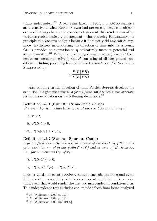
tically independent.33 A few years later, in 1961, I. J. Good suggestsan alternative to what Reichenbach had presented, because he objectsone would always be able to conceive of an event that renders two othervariables probabilistically independent – thus reducing Reichenbach’sprinciple to a vacuous analysis because it does not yield any causes any-more. Explicitely incorporating the direction of time into his account,Good provides an expression to quantitatively measure potential andactual causation.34 With E and F being distinct events (E and F theirnon-occurrences, respectively) and H consisting of all background con-ditions including prevailing laws of nature the tendency of F to cause Eis expressed by
logP (E |FH)
P (E |FH).
Also building on the direction of time, Patrick Suppes develops thedefinition of a genuine cause as a prima facie cause which is not spuriousresting his explication on the following definitions:35
Definition 1.5.1 (Suppes’ Prima Facie Cause)The event Bt′ is a prima facie cause of the event At if and only if
(i) t′ < t,
(ii) P (Bt′) > 0,
(iii) P (At|Bt′) > P (At).
Definition 1.5.2 (Suppes’ Spurious Cause)A prima facie cause Bt′ is a spurious cause of the event At if there is aprior partition πt′′ of events (with t′′ < t′) that screens off Bt′ from At,i. e., for all elements Ct′′ of πt′′
(i) P (Bt′Ct′′) > 0,
(ii) P (At′ |Bt′Ct′′) = P (At′ |Ct′′).
In other words, an event genuinely causes some subsequent second eventif it raises the probability of this second event and if there is no priorthird event that would render the first two independent if conditioned on.This independence test excludes earlier side effects from being analyzed
33Cf. [Williamson 2009, p. 189].34Cf. [Williamson 2009, p. 191].35Cf. [Williamson 2009, pp. 191 f.].

12 Reasoning about causation
as true causes. The same idea underlies the analysis of causation putforward by econometrician and Nobel Prize winner Clive Granger in1969, who argues for defining causes as events that are correlated withlater effect events only when the entire past history of the putative causeup to its very occurrence is held fixed, i. e., when all variables prior tothe cause candidate are conditioned on.36
All these considerations open into the development of the concept ofBayesian networks formulated by Judea Pearl in the 1980s as the basisfor automated inference.37 One of the protagonists in the field of proba-bilistic accounts of causation is Wolfgang Spohn who like Suppes alsoemphasizes the direction of time as a prerequisite crucial to his account.Where Suppes in his reductionist approach can be seen as represent-ing causal pluralism, since he does not stipulate which interpretation ofprobability is to be preferred above others, Spohn makes the case forthe subjective interpretation of probability as personal degrees of belief.Thus following the original intentions of Thomas Bayes he goes one stepfurther and characterizes the relation of causation in its core by statingthat “Bayesian nets are all there is to causal dependence”38 – in otherwords, sufficiently rich Bayesian nets in causal interpretation togetherwith the causal Markov condition yield just the dependencies and in-dependencies we also expect in scientific or everyday causal reasoningand when interacting with our environment (see chapter 2 for a detailedpresentation of Bayes nets, the Markov condition, and their causal in-terpretation).
All arguments for probabilistic accounts of causation face substantialpoints of criticism. Nancy Cartwright makes out quite a list of crit-ical observations about (more or less refined) purely correlation-basedcausal analysis.39 Trying to get from probabilistic dependence to causaldependence one should be wary:
What kinds of circumstances can be responsible for a probabilisticdependence between A and B? Lots of things. The fact that Acauses B is among them: Causes produce their effects; they makethem happen. So, in the right kind of population we can expect thatthere will be a higher frequency of the effect (E) when the cause (C)
36Cf. [Cartwright 2001, sect. 3].37Cf. e. g. [Pearl 1982].38This quotation refers to the title of [Spohn 2000].39Cf. for this and the following [Cartwright 2004] and the detailed discussion in
[Cartwright 2001].

Reasoning about causation 13
is present than when it is absent; and conversely for preventatives.With caveats.40
Among the issues Cartwright addresses is the fact that correlationmight be induced by common or correlated causes (or preventatives, re-spectively). Moreover, two causes might also – due to the fact that theyjointly produce an effect – be correlated in populations where the effectis strongly present (or absent, respectively), maybe because populationsare overstratified in the respective set-up of a study – i. e., in Bayesnet terminology, two otherwise causally unrelated variables are depen-dent conditional on a common successor in collider structures. Thirdly,certain variables may show the same time trend without being causallyrelated, at all. The prototypical example: The Venetian sea level riseswith the same tendency as does the bread price in London, althoughneither actually causes the other nor would we try to attribute the cor-relation to some latent common cause. Fourthly, one remark about theassumption of stability (sometimes also ‘faithfulness’): The informationconveyed by Bayes nets is actually encoded in the absences of directededges through which pairwise (conditional) independence between twovariables is indicated. Especially when we try to build Bayes nets fromraw data, the assumption of stability tells us that if data does not signaldependency between two variables, we have no reason to neverthelessinsert an edge between the two corresponding nodes in our Bayes net.The underlying assumption is that it takes very precise values to cancelcorrelation where there actually are (physical etc.) mechanisms at work,and that such preciseness is rarely if ever found in imprecise disciplinesor in oftentimes necessarily inexact measurements. Still, the theoreticalpossibility exists that, e. g., positive and negative effects of a single factorneutralize, thereby obscuring causal influence. Cartwright illustratesthis point with Germund Hesslow’s canonical birth-control pill exam-ple: “The pills are a positive cause of thrombosis. On the other hand,they prevent pregnancy, which is itself a cause of thrombosis. Given theright weights for the three processes, the net effect of the pills on thefrequency of thrombosis can be zero.”41 In this example it might notonly be the case that data does not show dependency where we wouldnormally suspect causal mechanisms at work, but it might moreover bean important goal of medical research to achieve this very independenceand to delete dependency from data – still acknowledging the physical,physiological etc. processes in nature.
40Cf. sect. 4, From probabilistic dependence to causality, in [Cartwright 2001].41Cf. [Cartwright 2001, sect. 3].

14 Reasoning about causation
Jon Williamson extends Cartwright’s list in his critique of over-simplistic applications of the Principle of Common Cause and its im-plications. He points out once more that two positively or negativelycorrelated events do not have to be related causally but may instead be“related logically (e. g. where an assignment to A is logically complexand logically implies an assignment to B), mathematically (e. g. meanand variance variables for the same quantity are connected by a math-ematical equation), or semantically (e. g. A and B are synonymous oroverlap in meaning), or are related by non-causal physical laws or bydomain constraints. In such cases there may be no common cause toaccompany the dependence, or if there is, the common cause may failfully to screen off A from B.”42 Nancy Cartwright sums up thesecritical points in pragmatic fashion – rejecting the philosophical effort tounify the representation of causal relations she says:
The advice from my course on methods in the social sciences isbetter: “If you see a probabilistic dependence and are inclined toinfer a causal connection from it, think hard. Consider the otherpossible reasons that that dependence might occur and eliminatethem one by one. And when you are all done, remember – yourconclusion is no more certain than your confidence that you haveeliminated all the possible alternatives.”43
Supposed opponent Judea Pearl agrees with Cartwright on thefact that the shortcomings of a purely probabilistic reductionist approachtowards causal analysis prohibit at least direct application. He marks thedistinction between mere observation (or acts) represented in data andknowledge about the impact of (hypothetical) intervention (or action)which is not part of statistical models. Conditioning on certain variablesjust switches the subpopulation and does not yield information about thecausal machinery at work.44 Obviously, a modification of the method isnecessary to also encode counterfactual knowledge.
1.6 Counterfactual analysis
One of the first references to the idea of characterizing causation in termsof counterfactual conditionals dates back to as early as 1748, when DavidHume compactly analyzed a cause to be “an object followed by another,
42Cf. [Williamson 2009, p. 200].43Cf. [Cartwright 2001, sect. 5].44Cf. e. g. the section Actions, Acts, and Probabilities in [Pearl 2009, pp. 108 ff.].

Reasoning about causation 15
[...] where, if the first object had not been, the second never had ex-isted.”45 Suzy throws a stone and shatters a window with it. Had shenot thrown the stone, the window would not have broken to pieces.Obviously, this counterfactual analysis seems to capture much of our in-tuition about causation. It ties the observed course of events – whenconsidering causal relations at token level – to the mechanisms that gov-ern our world underneath the surface and are of more use to us thanmere listings of successive happenings because they contain hints at howto manipulate the respective setting to achieve different outcomes. L. A.Paul notices that “[i]n everyday life as well as in the empirical and so-cial sciences, causes are identified by the determination of manipulation:Cs are causes of Es if changing Cs changes the Es, that is, if we canmanipulate Es by manipulating Cs. In this way, experimental settingsare designed to test for the presence of causation by testing for the pres-ence of counterfactual dependence.”46 In his seminal article Causation(1973) David Lewis offers a detailed presentation of causal analysis onthe basis of counterfactual dependence together with a full-blown seman-tics for evaluation.47 For him, counterfactual dependence between twosuccessive and suitably distinct events is sufficient for causation. But hispossible worlds semantics of counterfactuals does not yield transitivityof counterfactual statements in contrast to our intuition that causationshould be characterized as transitive. Thus, causation cannot be simplyreduced to counterfactual dependence. In the following, three notori-ous prima facie problematic cases shall be considered and possible fixesthereof sketched in brief – namely the cases of side effects, pre-emptedpotential causes, and overdetermined events.48
C
E
D
Fig. 1.1: D counts as side effect of E in this common cause fork.
45This is actually the second part of his famous twofold explication – see below,chapter 2, and cf. [Hume 1748, Section VII].
46Cf. [Paul 2009, p. 166].47Cf. [Lewis 1973b].48Cf. for this and the following the extensive discussion in [Paul 2009, sects. 2–3].
16 Reasoning about causation
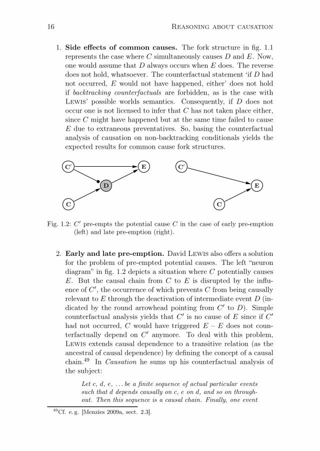
1. Side effects of common causes. The fork structure in fig. 1.1represents the case where C simultaneously causes D and E. Now,one would assume that D always occurs when E does. The reversedoes not hold, whatsoever. The counterfactual statement ‘if D hadnot occurred, E would not have happened, either’ does not holdif backtracking counterfactuals are forbidden, as is the case withLewis’ possible worlds semantics. Consequently, if D does notoccur one is not licensed to infer that C has not taken place either,since C might have happened but at the same time failed to causeE due to extraneous preventatives. So, basing the counterfactualanalysis of causation on non-backtracking conditionals yields theexpected results for common cause fork structures.
C′
C
E
D
C′
C
E
Fig. 1.2: C′ pre-empts the potential cause C in the case of early pre-emption(left) and late pre-emption (right).
2. Early and late pre-emption. David Lewis also offers a solutionfor the problem of pre-empted potential causes. The left “neurondiagram” in fig. 1.2 depicts a situation where C potentially causesE. But the causal chain from C to E is disrupted by the influ-ence of C ′, the occurrence of which prevents C from being causallyrelevant to E through the deactivation of intermediate event D (in-dicated by the round arrowhead pointing from C ′ to D). Simplecounterfactual analysis yields that C ′ is no cause of E since if C ′
had not occurred, C would have triggered E – E does not coun-terfactually depend on C ′ anymore. To deal with this problem,Lewis extends causal dependence to a transitive relation (as theancestral of causal dependence) by defining the concept of a causalchain.49 In Causation he sums up his counterfactual analysis ofthe subject:
Let c, d, e, . . . be a finite sequence of actual particular eventssuch that d depends causally on c, e on d, and so on through-out. Then this sequence is a causal chain. Finally, one event
49Cf. e. g. [Menzies 2009a, sect. 2.3].

Reasoning about causation 17
is a cause of another iff there exists a causal chain leadingfrom the first to the second.50
The so-called case of late pre-emption faces a different kind of prob-lem. If the right diagram of fig. 1.2 is interpreted as a series ofevents succeeding one another in time from left to right then eventC ′ prevents C from becoming causally effective by causing eventE earlier. To give an illustrative example: Suzy and Billy throwstones to shatter a glass bottle. Suzy’s stone hits the bottle earlierthan Billy’s and thus can be counted as the cause of the breakingof the bottle, whereas Billy’s stone must fail to break the bottle be-cause it is already broken to pieces. In this case (potential) causalefficacy of either event C or C ′ cannot be accounted for in terms ofcounterfactual dependence or causal chains. One way to side-stepthis problem is to introduce a fine-grained concept of events and tomake events fragile with respect to time.51 This makes counterfac-tual dependence applicable again: Suzy’s throw caused the bottleto break at time t1 – call this event Et1 . Had she not thrown thestone, the bottle would have broken later, at time t2, as event Et2
brought about by Billy’s throw. Et1 would not have occurred eitherin this case, thus validating the counterfactual ¬C ′ 2→ ¬Et1 .
52
The question remains, if this kind of fine-graining still captureseveryday causal talk, not to mention type-case utterances.
E
C
C′
Fig. 1.3: C and C′ overdetermine the event E in this collider structure.
3. Cases of overdetermination. A slightly modified variant ofthe bottle shattering example can be used to illustrate the casein which two events jointly overdetermine a later third event, assketched in the neuron diagram of fig. 1.3. Assume that Suzy (C ′)
50Cf. [Lewis 1973a, p. 563].51Cf. [Menzies 2009a, sect. 4].52The counterfactual formula in words: ‘If C′ did not occur, Et1 would not occur,
either’ (or the respective past tense form); see chapter 2 for an explication of thetruth conditions of counterfactuals.

18 Reasoning about causation
and Billy (C) throw their stones and hit the bottle at the exactsame time, causing it to break (E). Again, this situation cannotbe analyzed in accordance with our intuition if one relies on plaincounterfactual dependence. If either C or C ′ had not occurred, therespective remaining event would have caused the bottle to break.Resorting to temporally fragile interpretations of the situation doesnot remedy things either, because – as the example goes – bothstones simultaneously hit the bottle. Of course it might be arguedthat there are no genuine simultaneous events and that a sufficientfine-graining of the physical description of the situation will alwaysultimately yield a solution when drawing on the temporal fragilityof events or – going one step further – on an extension of fragilityto properties in general. So the interesting questions arise whenwe allow for fine-grained overdetermination53 and ask ourselveswhat the actual cause of a truly overdetermined event (also in thefine-grained sense) really is. This sounds like a tough questionin such an abstract formulation, and, e. g., L. A. Paul finds itnoteworthy “how differently we feel about the clarity of cases offine-grained overdetermination versus that of cases of early andlate pre-emption. [. . . ] it just isn’t clear how each cause is bringingabout the effect all on its own, given that another cause is alsobringing about the effect all on its own and the causation is notjoint causation.”54
One further general problem counterfactual theories of causation faceis the charge of circularity. If the definition of causal dependence rests oncounterfactual dependence, the semantics of counterfactuals must avoidrelying on causal relations. If this is not possible, more has to be saidabout the grounding of higher level on lower level causal claims or basiccausal assumptions (as do Woodward55 and Pearl56).
Although the counterfactual analysis seems to truly capture essentialfeatures of our understanding of causal relations, refined approaches areneeded, obviously. E. g., Judea Pearl proposes directed structural equa-tions and claims that these are actually expressions of counterfactual
53For a discussion of variants of fine-graining and overdetermination cf. [Paul 2009,pp. 178 ff.].
54Cf. [Paul 2009, p. 180]; joint causation means that both causes are needed tobring about the effect in the precise way it actually occurred.
55Cf. [Paul 2009, p. 172].56Cf. [Halpern & Pearl 2005a, p. 849].

Reasoning about causation 19
knowledge.57 On a higher level he even defines how to interpret theprobability that an event X = x “was the cause” of an event Y = y interms of counterfactuals: P (Yx′ = y′|X = x, Y = y) can be understoodin his framework as the probability of Y not being equal to y had X notbeen x, given that X = x and Y = y are (observed) facts in the respec-tive situation. Relative to his definition of probabilistic causal models,Pearl lists the three steps necessary for counterfactual evaluation (incorresponding twin networks): abduction, action (i. e., intervention), andprediction.58
Another contribution to the ongoing discussion – especially for thesolution of cases of overdetermination – has been brought forward byChristopher Hitchcock, who enhances structural representations oftest cases by introducing default and deviant values, thus emphasizingour intuition that an event is more likely attributed causal efficacy ifit deviates from the normal course of events in a sufficiently significantway.59 The semantics of normality nevertheless remains a point of con-troversy, as does the semantics of counterfactuals in the possible worldspresentation due to troublesome transfer into application, as, e. g., JudeaPearl points out insistently.60
1.7 Ranking theory
Another critic of the counterfactual account of causation (especially aspresented by Lewis) calls its self-imposed claim of objectivity in ques-tion. Wolfgang Spohn derives in his own approach causes from reasonsas subjective degrees of belief, thereby relativizing causation to an ob-server or epistemic individual. He criticizes Lewis:
[T]he stance of the counterfactual theory towards the objectivityissue is wanting, I find. The official doctrine is, of course, thatthe counterfactual theory offers an objective account of causation;this definitely counts in its favor. However, this objectivity gets ab-sorbed in the notion of similarity on which Lewis’ semantics forcounterfactuals is based. [. . . ] I wonder whether such similarityjudgments are significantly better off in the end than, say, judg-ments about beauty, and hence whether the semantics for coun-terfactuals should not rather take an expressivist form like the
57Cf. [Pearl 2009] and a presentation of Pearl’s framework in chapter 2.58Cf. [Pearl 2009, p. 206], Theorem 7.1.7.59Cf. e. g. [Hitchcock 2009a] and [Hitchcock 2007].60Cf. Pearl’s reply to Lewis’ article Causation in [Pearl 2009, pp. 238 ff.].

20 Reasoning about causation
semantics of “beautiful”. The question is difficult to decide, andI do not want to decide it here. The only point I want to makeis that the whole issue is clouded behind the objectivistic veil ofthe counterfactual theory. It is clearer, I find, to jump right intosubjectivity [. . . ] 61
Consequently, Spohn bases his account of causal reasoning on weight-ings of personal reasons in the form of ranking functions. Other thanpurely qualitative representations of epistemic entities (or changes insuch entities, respectively) in the area of knowledge representation orreasoning with uncertainty, ranking functions quantitatively representthe epistemic state of a subject in terms of degrees of belief, but at thesame time induce a notion of yes-or-no belief complying with the con-straints of rational reasoning (i. e., consistency and deductive closure).62
Only a very brief sketch of ranking theory shall be given here to sup-port the following points. A belief function β measures the strengthof an agents subjective belief in proposition A, depending on whetherβ(A) > 0 (belief in the truth of A), β(A) < 0 (belief in the falsity ofA), or β(A) = 0 (indifference as to whether A is true or false), withβ(A) ∈ Z ∪ −∞,+∞.63 Now, in this framework A is defined as a rea-son for B, iff β(B|A) > β(B|A), i. e., (the occurrence or the perceptionof) A strengthens the belief in B.64 Moreover, reasons are systematicallyclassified as additional, sufficient, necessary, or weak reasons, dependingon whether β(B|A) yields a value below or equal to 0 (in the cases ofA being a sufficient, necessary, or weak reason for B), whether β(B|A)yields a value above or equal to 0 (in the case of A being an additional,a sufficient, or necessary reason for B), and how these conditions arecombined.65 In a next step, causes are quite simply derived from thedefinition of reasons: A is an (additional, sufficient, necessary, or weak)direct (token or singular) cause of B iff (i) A is an (additional, sufficient,necessary, or weak) reason for B, (ii) A and B actually obtain, and (iii)A temporally strictly precedes B.66 Quite like Lewis, Wolfgang Spohn
goes on by defining a cause to be a proposition A that is connected toanother proposition B by a chain of direct causes. This is – in a nutshell
61Cf. [Spohn 2001, sect. 8].62Cf. [Huber 2009, p. 1351].63Cf. for this and the following e. g. [Spohn 2001].64This is of course formulated relative to (i. e., conditional on) an agent’s given
doxastic state C, which is omitted here for purposes of compactness.65Cf. [Spohn 2001, sect. 4], definition 5b.66Cf. [Spohn 2001, sect. 5], definition 6.

Reasoning about causation 21
– all that is needed to follow Spohn’s comparison of how cases of overde-termination can be treated in Lewis’ purely counterfactual account andin his own ranking-theoretic analysis.
If numbers are distributed in accordance with our understanding ofthe situation depicted in fig. 1.3, we could possibly come up with thefollowing tables showing concrete values for β(C|X ∩ Y ):67
β(C|·) B B
A 1 −1
A −1 −1
(a) A and B are jointsufficient and joint nec-essary causes
β(C|·) B B
A 1 0
A 0 −1
(b) A and B are jointsufficient but not neces-sary causes
β(C|·) B B
A 2 1
A 1 −1
(c) A and B are overde-termining causes of C
Each table specifies the degree of belief β(C|X ∩ Y ) in C conditional onX ∩ Y , where X ∈ A,A and Y ∈ B,B. Numerical values possiblechange from one epistemic subject to another (under preservation ofnecessity, sufficiency, or overdetermination if constrained correctly).
Case (a) represents the standard understanding of joint causes – both Aand B have to occur in order to bring about C, neither A nor B alonesuffice for that, given through β(C|A∩B) > 0 > β(C|A∩B) = β(C|A∩B) = β(C|A∩B). Only the joint occurrence of A and B raises the beliefin C from a negative number (disbelief) to a positive (belief).
Spohn also considers case (b) an example of joint causation, obviouslynot as definite as case (a) since, e. g., in the presence of A the occurrenceof B is (per definitionem) a sufficient contribution to C, but a necessaryone in the absence of A: β(C|A ∩B) > 0 = β(C|A ∩B) > β(C|A ∩B).The occurrence of either A or B raises the belief in C from disbelief (< 0)to indifference (= 0), but only the joint occurrence of A and B lifts thedegree of belief in C to a positive value.
Scheme (c) finally exhibits the case of overdetermining causes. Each ofA and B already suffices to produce C by raising the belief in C froma negative to a positive degree and can be understood as an additionalcontribution to C in the presence of the other, raising the degree of
67This example is taken from Spohn’s illustration of the problem of overdetermi-nation in [Spohn 2001, sect. 7].

22 Reasoning about causation
belief in C even further, as specified in the ranking function β and giventhrough β(C|A∩B) > β(C|A∩B) = β(C|A∩B) > 0. The high degreeof belief in C can be interpreted as strong doubt in the fact that C wouldobtain if neither of A or B actually occurred.
Wolfgang Spohn summarizes why ranking theory copes with the fine-grained representation of causal intuitions much better than the coun-terfactual approach:
[R]anking functions specify varying degrees of disbelief and thusalso of positive belief, whereas it does not make sense at all, incounterfactual theories or elsewhere, to speak of varying degrees ofpositive truth; nothing can be truer than true. Hence, nothing cor-responding to scheme (c) is available to counterfactual theories.68
Nevertheless, justified questions appear on the scene as soon as one triesto tie ranking theory to application, e. g., in implementations of beliefrevision or automated reasoning. How does an epistemic agent obtainthose specific numerical values as initial degrees of belief? And if rank-ing theory starts constructing singular causes from subjective reasons –how, if at all, could any notion of objectivity be established?69 Andthe computer science engineer might add: Isn’t there any more compactway of representing and implementing degrees of belief and changes ofepistemic states than as plain listings of each and every ratio?
1.8 Agency, manipulation, intervention
Manipulationist theories of causation build upon our very basic intuitionthat an effect can be brought about by an apt manipulation of the puta-tive cause. In other words and cum grano salis, if an event C causes somedistinct event E, then a modification of C in some way will change theoutcome E correspondingly. And conversely, if by (if only hypothetical)manipulation of an event C some subsequent event E were to presentitself differently (relative to the expected normal and unmanipulatedcourse of events), C causes E (even if in this counterfactual formulationthe manipulation were not actually to be performed). This idea has re-ceived considerable attention in the recent literature on causal inference,even in non-philosophical publications of medical research, econometrics,
68Cf. [Spohn 2001, sect. 7].69Of course, Spohn does say more about the task of objectivizing ranking functions
e. g. in [Spohn 2001] and [Spohn 2009].

Reasoning about causation 23
sociology, even psychology and molecular-biology etc. because it mapsthe quest for causes onto the practice of experimentation. Manipulation-ist theories in this way go beyond the determination of mere regularitiesin observed processes or the plain investigation of correlation, and intro-duce the (virtual) capability of interaction into the test setting. This isdone differently in different flavors of manipulationist theories.70 Agencytheories in anthropomorphic fashion emphasize an agent’s freedom of ac-tion involved in performing a manipulation of the respective situation.The gap between (human) agency and causation is then bridged by thenotion of agent probability. The causal efficacy of an event C on E islinked to C’s raising the agent probability of E, when this agent prob-ability is interpreted as the probability that E would obtain if an agentwere to choose to realize C. Since in this formulation causation is brokendown into atomic building blocks of free acts, agency theories do avoidcircularity – they face a different problem, though, namely their verylimited scope of application. E. g., how is causal efficacy attributed tofriction of continental plates resulting in an earthquake? Surely we uttercausal claims about such geo-physical happenings with the same confi-dence as we talk about someone’s throwing a stone as being the cause ofsome bottle’s shattering.71
Judea Pearl72 or James Woodward
73 draw on a different and moregeneral kind of manipulation. In their congeneric accounts of causationthe capability of interaction is given through hypothetical interventionson variables in fixed causal models. Those variables are basically suitablydistinct events of interest that the designer of a causal model deemsto be worth considering and contributory to the understanding of therespective situation. Causal models moreover – in essence – merely listfor each variable in the model its immediate predecessors, i. e., causallyinterpreted, its direct causes (thus obeying the so-called causal Markovcondition if the resulting structure does not contain cycles of parenthood,see below, definition 2.6.1). The underlying idea of both Pearl’s andWoodward’s approach is modularity as a requirement for causal modelsto be reliable sources of information and thus useful for explanation.
70Cf. for this and the following [Woodward 2009].71See Woodward’s discussion of the earthquake example due to Menzies and
Price together with the potential but controversial solution via projection in [Wood-ward 2009, pp. 238 ff.].
72Cf. [Pearl 1995] and for a more elaborate presentation [Pearl 2009] (the secondedition of his 2000 book).
73Cf. [Woodward 2003].

24 Reasoning about causation
Modularity accounts rest on the postulate that each link between twovariables represents a mechanism for the effect, which can vary modularlyand independently of mechanisms for any other variables in the causalmodel.74 If those mechanisms are represented as individual equations,the researcher can mathematically utilize them to learn about the effectsof interventions – as Pearl puts it:
In summary, intervention amounts to a surgery on equations[. . . ] and causation means predicting the consequences of sucha surgery.75
Nevertheless, how such interventions are precisely implemented inPearl’s and Woodward’s account slightly varies in detail. Pearl
compactly defines atomic interventions as external deactivations of somevariable’s links to its causal parents (i. e., its direct causes) or analogouslyas the deletion of the respective functional connection in the correspond-ing structural model:
The simplest type of external intervention is one in which a singlevariable, say [X], is forced to take on some fixed value [x]. Suchan intervention, which we call “atomic”, amounts to lifting [X]from the influence of the old functional mechanism [linking thevalue assignment of X to the values of its parents] and placing itunder the influence of a new mechanism that sets the value [x]while keeping all other mechanisms unperturbed.76
As Woodward notes critically, this explication induces a definition ofcause that relies on certain mechanisms to remain unperturbed. If thesemechanisms are of causal character themselves, then Pearl has to de-fend his definition against the charge of circularity. He indeed does sug-gest a possible reading of interventions that avoids circularity in [Halpern& Pearl 2005a]. (For a detailed presentation of Pearl’s account of cau-sation see chapter 2.) Woodward follows a slightly different route byintroducing specific intervention variables into his framework and by con-straining those variables in a suitable way. An intervention I on somevariable X is then defined relative to the putative effect Y in order tocharacterize what it means for X to cause Y :77
74See [Cartwright 2004, pp. 807 ff.] for a critical discussion of the modularityrequirement.
75Cf. [Pearl 2009, p. 417] – highlighting modified.76Cf. [Pearl 2009, p. 70].77See Woodward’s presentation of the requirements of such Woodward-
Hitchcock interventions in [Woodward 2009, p. 247].

Reasoning about causation 25
1. I must be the only cause of X – i. e., the intervention must com-pletely disrupt the causal relationship between X and its precedingcauses so that the value of X is entirely controlled by I (in otherwords, the set of parents of X only contains I);
2. I must not directly causally influence Y via a route that does notgo through X;
3. I should not itself be caused by any cause that influences Y via aroute that does not go through X;
4. I must be probabilistically independent of any cause of Y that doesnot lie on the causal route connecting X to Y .
In contrast to Pearl’s explication, it is not excluded that such an in-tervention variable I is causally related to or probabilistically dependenton other variables in the causal model, but it is specified exactly, whichvariables I is required to be (causally and probabilistically) independentof. And in contrast to agency theories, as Woodward emphasizes, a“purely natural process, not involving human activity at any point, willcount as an intervention as long as it has the right causal and correla-tional characteristics.”78
The pivotal idea of modular manipulationist accounts is the exploita-tion of causal diagrams for reliable causal inference. The Bayes netmethodology provides the desired framework and readily extends causalyes-or-no reasoning to an analysis of causal influence in terms of degreesof belief. Mapping this approach onto the standard proceeding of a ran-domized controlled clinical trial exemplifies the general applicability ofinterventionist theories.
I
S1
C
S2
Fig. 1.4: Symptom S1 is lifted from the causal influence of cause C by meansof intervention I in a randomized controlled trial.
78Cf. [Woodward 2009, p. 247].

26 Reasoning about causation
Consider the situation depicted in figure 1.4 where some cause C (per-haps some disease or some behavior detrimental to health) results in thesimultaneous occurrence of symptoms S1 and S2.
79 Arrows mark directcausal influence. In order to discover the causal relationship betweenC, S1, and S2, the test candidates (exhibiting characteristic c or ¬c inthe dichotomous case) are divided randomly into test groups (subpop-ulations) where in one group symptom S1 is induced somehow and inthe other group prevented – according to the decision taken by settingI. Now, if inducing or preventing symptom S1 were to bring about asignificant change in the measurement of symptom S2, we would be en-titled to postulate some causal connection between both variables dueto the above explication of intervention. Randomization of test groupsnevertheless precisely amounts to lifting the variable S1 from the influ-ence of variable C and cutting the connection (thereby cancelling thecorrelation) between S1 and C (as indicated by the dashed arrow point-ing from C to S1 in figure 1.4) and consequently between S1 and S2. S1
is therefore analyzed as not directly causally influencing S2.The example makes obvious how tightly the principle of modularity isconnected with causal reasoning – without the assumption of modular(and modularly separable) causal links the whole enterprise of random-ization in our controlled clinical trial would have failed. Another inves-tigation Woodward undertakes in the explication of his interventionistaccount is centered about the question, what the nature of mechanismsis in essence. He reminds the reader of his Making Things Happen (2003)of “the absence of any consensus about the criteria that distinguish lawsfrom nonlaws and the difficulties this pose[s] for nomothetic accountsof explanation”80 and discusses invariance as an intrinsic feature of thegeneralizations required for causal inference, thereby strengthening themodularity requirement:
The guiding idea is that invariance is the key feature a relationshipmust possess if it is to count as causal or explanatory. Intuitively,an invariant relationship remains stable or unchanged as variousother changes occur. Invariance, as I understand it, does not re-quire exact or literal truth; I count a generalization as invariantor stable across certain changes if it holds up to some appropri-ate level of approximation across those changes. By contrast, ageneralization will “break down” or fail to be invariant across cer-tain changes if it fails to hold, even approximately, under thosechanges.81
79This illustration follows the motivational example in [Woodward 2009, sects. 2/5].80Cf. [Woodward 2003, p. 239].81Cf. [Woodward 2003, p. 239].

Reasoning about causation 27
Woodward goes on by bridging the gap between his theoretical claimsand (the practice of) explanation in the special sciences:
In contrast to the standard notion of lawfulness, invariance iswell-suited to capturing the distinctive characteristics of explana-tory generalizations in the special sciences. [. . . ]
[A] generalization can be stable under a much narrower range ofchanges and interventions than paradigmatic laws and yet stillcount as invariant in a way that enables it to figure in explana-tions.82
In her critical discussion, Nancy Cartwright acknowledges the ad-vantages of invariance methods but also points out that these methodsrequire a great deal of antecedent causal assumptions or knowledge aboutthe causal influences at work, because what it means for some generaliza-tion to be invariant or stable across certain changes of the right sort mustcarefully be explicated when applying the method to individual causalhypotheses. Due to these demanding requirements, Cartwright ar-gues, invariance methods “are frequently of little use to us.”83 Anotherreason for her to object to invariance methods is the fact that the sit-uation under consideration must be of modular nature, which is – inCartwright’s eyes – only the case for a limited set of situations anddoes not carry over to general application.84 Pearl refutes this argu-ment sharply in [Pearl 2010] by claiming that formal structural systems(e. g., as used in econometrics) are usually established on the basis ofthe modularity assumption.85 Woodward (necessarily) bases his in-terventionist notion of causation precisely on the modularity principleand defines what it means for an event to be a direct cause of someother subsequent event through combination of multiple interventions asfollows:
Definition 1.8.1 (Woodward’s Direct Cause)86
A necessary and sufficient condition for X to be a direct cause of Y withrespect to some variable set V is that there be a possible intervention I
on X that will change Y (or the probability distribution of Y ) when allother variables in V besides X and Y are held fixed at some value byadditional interventions that are independent of I.
82Cf. [Woodward 2003, p. 240].83See Cartwright’s critical discussion in [Cartwright 2004, pp. 811 f.].84Cf. [Cartwright 2004, pp. 807 ff.].85Cf. [Pearl 2010, pp. 73 ff.].86See definition (DC) in [Woodward 2009, p. 250].

28 Reasoning about causation
Using this definition as a starting point for further considerations, con-ditions for X to be a contributing cause of Y are consequently built onthe notion of chains of direct causes. How Judea Pearl uses the notionof intervention in his framework and how he ultimately arrives at theconcept of actual cause is presented in more detail in chapter 2.
1.9 Decisions to take
The brief presentation of manipulationist strategies concludes the sys-tematic overview of the most prominent approaches towards the analysisof causal claims. Obviously, the different approaches more or less differin their attempt to provide answers to a set of questions that are centralto the analysis of causation. The most important decisions one has totake when setting out to trace the notion of causality in some way shallbe collected in the following catalogue.87
1. What are the relata of causal relations? Can objects or regions oftime-space be the cause of entities of the same kind? Or does anycausal talk of objects always have to be understood in terms of themore fundamental concept of events, i. e., either as instantiationsof properties in objects at a given time (in the Kimian sense) oras plain random variables (in a probability-theoretic sense) thatsignify events by assuming one of at least two different values?
2. Does the causal analysis in the framework to be developed relatesingle case entities (at token level) or does it ascribe meaning toclaims about generic causation (at type level)? If both cases aretreated in the framework – which one is prior to the other? Arecases of singular causation as “the rain yesterday at noon causedmy driveway to get wet” to be understood as more fundamentalthan cases of generic causation as “rain causes a street to get wet”– or vice versa? And can one be derived from the other, e. g., bysome kind of induction principle?
3. Do causal claims relate entities at population level or at individ-ual level? E. g., a certain approach might be able to deal wellwith medical findings connecting some epidemic in a given groupwith the presence of some virus but might fail to account for the
87This compilation expands the listings in [Williamson 2009, pp. 186 f.] and [Paul2009, pp. 160–165].

Reasoning about causation 29
outbreak of a disease in a specific observed individual. The ex-planatory power of a causal theory must be balanced well if it isto deal with up-scaling or down-scaling of test settings.
4. Is the theory capable of explicating actual causation (maybe postfactum) or potential (possible, but maybe, e. g., pre-empted) cau-sation? This question is obviously closely connected to the ques-tion, if the theory can handle counterfactual intuitions and yieldanswers to queries of the what-would-have-happened-if-things-had-been-different kind (possibly by ascribing causal efficacy to factu-ally void, disrupted, or prevented events).
5. What is causation grounded in ontologically? Is the theory to bedeveloped talking about some objective, physical notion of causa-tion or about subjectively perceived or reconstructed mental cau-sation within an (idealized) epistemic agent? And if both alter-natives are not exclusive – how can knowledge about one side becarried over to the other side? If the subjective notion is prior tothe objective one – how, if at all, is objectivization possible? More-over, causal explanation clearly seems to be mind- and description-dependent. Now, if causation itself is of epistemic nature – whatthen is the difference between causal explanation and causation, ifthere is one to be made out?
6. Does the suggested account explore causation conceptually or onto-logically? In other words, does it present an analysis of how we gainepistemic access to causal relations and how we internally structureour experience of causal processes, or is the account attempting togive an insight into what really is at the core of causation in theworld? And if a conceptual approach does not deny the metaphys-ical existence of causal goings-on – how can the interconnectionbetween both be described?
7. Is the approach taking a descriptive or a prescriptive route, i. e.,is the account offering an illuminative picture of our concept ofcausation (via description) or is it prescriptively focusing on theconstruction of an improved formulation – maybe in a technicallystrongly constrained framework or for a certain branch of the spe-cial sciences?
8. Is causation holistically treated as one monolithic concept suchthat a technical description of causal relations can be applied toany kind of causal claims, independent of research area or jargon?
30 Reasoning about causation
Or is ‘causation’ rather understood as a sort of cover term for thedescription of an irreducible multifarious, yet family-like concep-tion?
9. If causation is understood as a family of different concepts thatare best not reduced to allow for a better understanding of eachof the single concepts – then which of the concepts is analyzed bythe theory (if an analysis is attempted)? Is it the folk concept,the scientific concept, or possibly even the concept of a specialbranch of science? Does the theory approach causation from thephilosophical or epistemological perspective? And moreover, how(if at all) are thought experiments, personal intuitions (as aboutcases of causation by omission), causal talk as linguistic expression,or special physical theories addressed?
10. Are causal relations themselves reduced to other non-causal morefundamental entities or in a non-reductive approach seen as the ba-sic building blocks of causal claims? What could be candidates formore fundamental non-causal entities – powers, processes, mecha-nisms? And to pose a question closely connected to the problemof reducibility: How are the laws of physics to be understood andhow (if at all) are they allocated in the framework?
11. Another important question marks the distinction between, e. g.,Pearl’s account of causation and Spohn’s ranking-theoretic ap-proach: What role does time play for the identifiability of causesand effects? Is time induced by the formal representation of cause-effect relations? Is it at best compatible with the arrangement ofcausally connected events? Or is it even seen as a necessary pre-requirement that might ultimately go into the definiens of causalrelations? And one more notorious question a theory of causationshould be addressing: Is backward causation something worth con-sidering, is it explicitly excluded from treatment or even denied bythe framework?
12. Does an account of causation refer to deterministic causal relationsor to probabilistic causation? And if it does talk about probabilisticcausal relations – in what sense are these causal relations proba-bilistic, in a genuinely ontologically aleatoric sense or (in an epis-temic sense) simply as a feature of our shortcoming to model sup-posed deterministic processes in a deterministic way? And does theframework allow for going back and forth between the deterministic

Reasoning about causation 31
and the probabilistic rendition if both are addressed (maybe withone prior to the other)?
13. The final question is maybe one which is to be left to the evaluationof the theory as it proves itself in practice (or does not). It will bejustified to ask, how applicable the theory finally turns out to be.To what degree does the proposed definition of cause prove opera-tionally effective? How well can the suggested account be coupledwith existing frameworks – especially when trying to embed causalconcepts in the special sciences? The answer to these questions willobviously be related to the choice of the formal framework with itsnotation and the mathematical tools therein.
In chapter 3 below these questions will be reconsidered and relatedto an extension of the interventionist treatment of causation. It will beargued that causation be understood as an epistemic concept in order toilluminate certain disputed examples and controversial intuitions. Rea-soning about causation will lead to the conclusion that a formal under-standing of causal relations tells us more about the texture of reasoningitself. Our knowledge is – as will be argued – efficiently structured by theguiding principle of causality. It is such structured knowledge, mappedonto patterns of unified causal and non-causal information, which ulti-mately permits cognition causarum rerum.


Chapter 2
Causation and causality:From Lewis to Pearl
Truth, or the connectionbetween cause and effect, aloneinterests us. We are persuadedthat a thread runs through allthings; all worlds are strung onit, as beads
Ralph Waldo Emerson,Montaigne; or, the Skeptic
2.1 What is a theory of causation about?
Within the last forty years the literature about theories of causationhas increased immensely: Language analysts built new alliances withcomputer scientists and computational linguists. From this very cornerprobability theory was fueled, which bestowed upon philosophers thepossibility of thinking about probabilistic causality. Pearl himself isa computer scientist and as such eager to offer effective tools aiding infinding concrete solutions to concretely posed questions. He thus turnson the purely metaphysical non-treatment of the concept of causationand devises a causal-theoretic toolbox for economists, physicians, sociol-ogists – in short: for all those on the hunt for causes. At the same timehe analyzes the prevalent situation with the following words:

34 From Lewis to Pearl
Ironically, we are witnessing one of the most bizarre circles in thehistory of science: causality in search of a language and, simulta-neously, speakers of that language in search of its meaning.1
A theory of causation – however furnished – ought to be instrumentalto the user and yield answers to queries like these, at least in agreementwith personal intuition:2
• Is X a cause of Y ?
• Is X a direct (respectively, an indirect) cause of Y ?
• Does the event X = x always cause the event Y = y?
• Is it possible that the event X = x causes Y = y?
Lewis and Pearl share common grounds in acknowledging that ineveryday language stating causes is our base of explanation and justifi-cation, and that prediction of future events intrinsically and inextricablyrests on causal assumptions. The analytical approaches deviate from oneanother, nonetheless.
2.2 Hume’s counterfactual dictum
David Lewis’ paper Causation in the Journal of Philosophy 1973 openswith Hume’s famous twin definition from 1748:
We may define a cause to be an object followed by another, andwhere all objects, similar to the first, are followed by objects similarto the second. Or, in other words, where, if the first object had notbeen, the second never had existed.3
The first part of this quote from David Hume’s An Enquiry About Hu-man Understanding, Section VII, sums up, what the regularity analysisof causation rests on. The mere uniform succession of events shall li-cense the observer to identify an event occurring (or is it only beingobserved?) before a second event as a genuine cause of this very secondevent. Here and in what follows I will only talk about ordinary events
1Cf. [Pearl 2009, p. 135] – a slight variation of his original formulation in [Pearl2000a, p. 135].
2Cf. [Pearl 2009, p. 222].3Cf. [Hume 1748, Section VII].

From Lewis to Pearl 35
to follow Lewis’ own self-restriction: Lightning in a thunderstorm, bat-tles between nations, chats amongst friends, etc. David Lewis formu-lates various critical notes against this regularity analysis of causation,thereby criticizing the advocates of probabilistic causality, who base theirtheory on the very correlation between events or states. In particular,any scenario exhibiting the regular succession of an event c (for cause)and an event e (for effect) can be analyzed reversely, so that – followingHume’s words – e counts as a genuine cause of c.4 This might possibly beagainst the arrow of time if time itself is not explained “into” the theory.Simultaneousness remains a tough case. Epiphenomena as echo of thecausal history of an event c cannot be distinguished from epiphenomenaof genuine effects e. And inefficacious pre-empted potential causes thatmight well have had causal influence, if not being pre-empted, are noteven touched by the regularity analysis.
As an alternative, Lewis turns to Hume’s “other words”: “If thecause c had not been, the effect e would not have occurred, either.”This “had not – would not” analysis constitutes one piece of the jigsawof David Lewis’ grand agenda of analyzing counterfactual statements,which culminates in his opus Counterfactuals, published in 1973, in thesame year as Causation. Lewis presses his point there:5
True, we do know that causation has something or other to do withcounterfactuals. We think of a cause as something that makes adifference, and the difference it makes must be a difference fromwhat would have happened without it. Had it been absent, its effects– some of them, at least, and usually all – would have been absentas well.
Years later Judea Pearl will argue in the same direction.
As a sole spoiler, the meaning of counterfactual statements seems toevade intuition at first sight. Lewis counters this the following way:
Why not take counterfactuals at face value: as statements aboutpossible alternatives to the actual situation, somewhat vaguelyspecified, in which the actual laws may or may not remain intact?
Lewis does take counterfactuals at face value and designs an appa-ratus for the evaluation of such statements in his book Counterfactuals.
4Cf. [Lewis 1973a, p. 557].5For this and the following cf. [Lewis 1973a, p. 557].
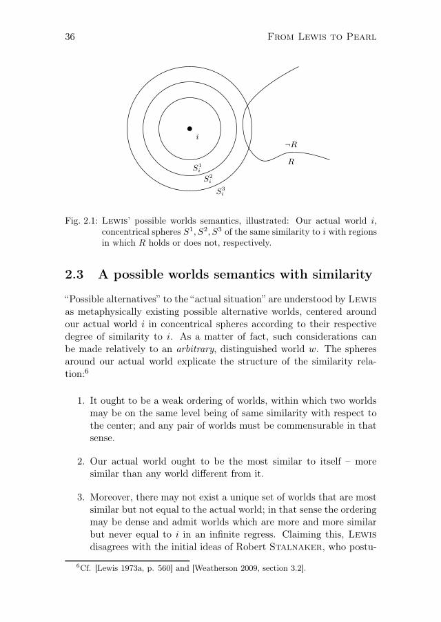
36 From Lewis to Pearl
S1
i
S2
i
S3
i
i¬R
R
b
Fig. 2.1: Lewis’ possible worlds semantics, illustrated: Our actual world i,concentrical spheres S1, S2, S3 of the same similarity to i with regionsin which R holds or does not, respectively.
2.3 A possible worlds semantics with similarity
“Possible alternatives” to the “actual situation” are understood by Lewis
as metaphysically existing possible alternative worlds, centered aroundour actual world i in concentrical spheres according to their respectivedegree of similarity to i. As a matter of fact, such considerations canbe made relatively to an arbitrary, distinguished world w. The spheresaround our actual world explicate the structure of the similarity rela-tion:6
1. It ought to be a weak ordering of worlds, within which two worldsmay be on the same level being of same similarity with respect tothe center; and any pair of worlds must be commensurable in thatsense.
2. Our actual world ought to be the most similar to itself – moresimilar than any world different from it.
3. Moreover, there may not exist a unique set of worlds that are mostsimilar but not equal to the actual world; in that sense the orderingmay be dense and admit worlds which are more and more similarbut never equal to i in an infinite regress. Claiming this, Lewis
disagrees with the initial ideas of Robert Stalnaker, who postu-
6Cf. [Lewis 1973a, p. 560] and [Weatherson 2009, section 3.2].

From Lewis to Pearl 37
lates a uniquely distinguished sphere of most similar worlds withhis Limit Assumption.
Any single of this possible worlds can be understood as an exhaustivestate description: If it is raining in our actual, world we find the claim R
to be true in the center i of our modeling. In some other world differingfrom ours with respect to the weather we would encounter ¬R. Typically,as the meaning of single claims like R or ¬R their respective worlds arebundled to propositions, i. e., sets of possible worlds.
The counterfactual statement “If φ had occurred, ψ would have occurredas well” may now be evaluated in possible worlds semantics:
φ 2→ ψ (2.1)
is true exactly if and only if there is no world in which φ ∧ ¬ψ holdsbeing closer to our actual world i than a world in which φ∧ψ holds. Orin David Lewis’ own words:
[...] a counterfactual is nonvacuously true iff it takes less of adeparture from actuality to make the consequent true along withthe antecedent than it does to make the antecedent true withoutthe consequent.7
And in formal fashion:
i φ 2→ ψ :⇐⇒ ¬hw(w φ) j (2.2)hu(u φ ∧ ψ k dv(v φ ∧ ¬ψ =⇒ v >i u))
,
for possible worlds w, u, v and the similarity relation ≤i with respect toour actual world i. The truth of the second disjunct of (2.2) depends onthe existence of some possible world u satisfying φ∧ψ and being closer toi than any φ∧¬ψ-worlds. This second disjunct is not formulated relativeto the φ∧ψ-worlds closest to i, because Lewis strictly rejects the LimitAssumption, i. e., the assumption that for any specific proposition thereis a unique set of worlds closest to some fixed actual i. Instead, therecould be closer and closer worlds (or narrower and narrower spheres ofpossible worlds, respectively) infinitesimally close to but never reaching¬(φ ∧ ψ) in a limitless infinite regress of refinement – in contrast to,e. g., Robert Stalnaker, who endorses the Limit Assumption in his
7Cf. [Lewis 1973a, p. 560].

38 From Lewis to Pearl
formulation of the truth conditions of counterfactuals.8 Moreover, inthe non-continuous finite and discrete case the truth of counterfactualscan always be evaluated deploying the limit assumption, because for anyproposition the i-closest worlds can be made out uniquely.
i
φ
ψ
b
Fig. 2.2: φ 2→ ψ is true at i if and only if there is no φ ∧ ¬ψ-world that iscloser to our actual world i than a φ ∧ ψ-world.
Formula (2.2) can be rephrased in set-theoretic notation so that thesimilarity relation ≤i with respect to the actual world i is representedby the hierarchy of cumulative spheres i, where Sn
i =⋃n
x=0 Sxi :
i φ 2→ ψ :⇐⇒⋃
i ∩ JφK = ∅ j (2.3)hS ∈ i
(
S ∩ JφK 6= ∅ k S ∩ JφK ⊆ JψK)
,
where JφK := u |u φ represents the worlds where φ holds (in otherwords, the proposition φ). Analogously to (2.2), this formulation doesnot postulate that there be the narrowest sphere S in which φ-worldscan be found, but holds true if there is a sphere S, at all, so that theφ-worlds within S are included in the set of ψ-worlds. If this is the case,then it already holds for the sphere with the φ-world most similar to i,since the similarity relation ≤i is represented in the cumulative hierarchyof i.
8See e. g. [Weatherson 2009, sect. 3.2] for a comparison of Lewis’ and Stal-
naker’s differing truth conditions of counterfactuals and Lewis’ discussion of theLimit Assumption in [Lewis 1973b, pp. 19 ff.].

From Lewis to Pearl 39
Two technical remarks shall once more illuminate potential border cases:9
1. If there is no world where the antecedent of the counterfactualis evaluated with truth value 1, the counterfactual statement isdefined to still hold vacuously – this is due to the first disjuncts of(2.2) or (2.3), respectively.
2. According to the formulations above, the counterfactual state-ment also includes the non-counterfactual case, i. e., where theantecedent φ already holds in our actual world. In this case thecounterfactual is true if and only if the mere material implicationwith the same sub-statements holds true. Accordingly, ψ must alsohold in our actual world.
Lewis’ critics are particularly aiming at his similarity measure whichhe ultimately employs to objectivize counterfactual statements: Whatare the criteria for such a measure? Does one not need to consider, inaddition to a given reference world, a certain aspect in question, withrespect to which one can speak of greater or smaller similarity betweenworlds? What is a manageable metric on this relation supposed to looklike? Is it not the case that any possible similarity assessment in thevery core rests on the subjective evaluation of one’s environment? Andhow is the following example to be analyzed?10
ExampleIf Richard Nixon had pushed the button, there would have been nuclearwar.
Does a world with a sole dysfunctional button resemble our actual worldto a greater degree than an alternative world in which we are facing a nu-clear catastrophe? Lewis allows insight into his conception in his paperfrom 1979, Counterfactual Dependence and Time’s Arrow, in which heequips the aspects of his similarity measure with priorities in imperativemanner:
1. It is of the first importance to avoid big, widespread, diverse vio-lations of law.
2. It is of the second importance to maximize the spatio-temporalregion throughout which perfect match of particular fact prevails.
9For this and the following cf. [Lewis 1973b, p. 16 ff.] and (in causal-theoreticcontext) also [Lewis 1973a, p. 560 f.].
10For the following cf. [Weatherson 2009, sect. 3.3].

40 From Lewis to Pearl
3. It is of the third importance to avoid even small, localized, simpleviolations of law.
4. It is of little or no importance to secure approximate similarity ofparticular fact, even in matters that concern us greatly.
With hindsight to this list of priorities, a world where all machineryof modern warfare targeted at nuclear destruction failed would resem-ble our actual world far less than the post-nuclear apocalypse. We arecertainly not having a hard time comparing worlds where logical neces-sities are overridden, where the laws of physics are suspended, or whereextensive geographical restructuring affects the environment. The ques-tion remains, if the proposed similarity measure over possible alternativeworlds is (i) natural, i. e., in accordance with our conceptualization, and(ii) to be understood as operationally effective in any way.
2.4 From counterfactual dependence to veritable
causes
To be able to identify causal relationships between clusters (i. e., sets)of events, David Lewis extends the counterfactual analysis to relation-ships between families of propositions.11 Now, if each two elements fromthese coupled sets of propositions are related counterfactually, we speakof counterfactual dependence between the respective sets of propositions.Typically, measuring processes as well as observation and control rou-tines are characterized by counterfactual dependence between large fam-ilies of alternatives: E. g., the family of alternative barometer readingscounterfactually depends on the family containing alternative values ofatmospheric pressure – under the assumption, the barometer works prop-erly, is calibrated correctly, not perturbed etc.
Without much hesitation Lewis reduces causal dependence (in any casebetween actual events such as lightning in a thunderstorm etc.) to coun-terfactual dependence between the according propositions (i. e., sets ofpossible worlds).
Hume’s counterfactual formulation – the second part of the twin defi-nition – thus parallels Lewis’ definition of causal dependence betweentwo events, not of causation itself. This dependence holds relative to thetruth of the following pair of counterfactuals:
11For this and the following cf. [Lewis 1973a, p. 561 f.].

From Lewis to Pearl 41
(i) φ 2→ ψ and
(ii) ¬φ 2→ ¬ψ.
Causal dependence (or its extension to causal chains, i. e., chains ofevents, where each event causally depends on the respective predeces-sor) between two specific events entails causation, according to DavidLewis. The reverse direction must not be taken for granted: Causationdoes not imply causal dependence, in general. Causation should be tran-sitive if it is to capture our intuitions, while this does not apply to causaldependence. Lewis be quoted here with his own example (illustrated infigure 2.3):
[...] there can be causation without causal dependence. let c, d,and e be three actual events such that d would not have occurredwithout c and e would not have occurred without d. Then c is acause of e even if e would still have occurred (otherwise caused)without c.
c
d
e
?
?
Fig. 2.3
“otherwise caused”? – The quote leaves thereader wondering, since the scenario, as stated,does not leave room for other causes, and thetwofold counterfactual analysis in the aboveformulation expresses precisely the necessarycausal succession c A d A e. So, how canLewis’ words be understood? Firstly, theexample is not to be understood as a self-contained story. It does not depict a closedworld situation with no potential external in-fluence. The strand c A d A e is to be seenas part of some metaphysically existing web ofcauses and effects that we have access to viareasoning and intuition. When we talk about
such scenarios we might very well agree on more causally influential en-tities that we deem relevant, e. g., for explanation. c remains a potential(but void) cause of an actually occurring event e, even if c is prevented orpre-empted by other obtaining circumstances. Secondly, Lewis strictlyrejects the possibility of backtracking counterfactuals. Knowledge aboutthe consequent does not tell us anything about the antecedent. This pre-cisely reflects the idea that the actual cause of an event may emerge fromthe abundance of potential cause candidates and override other (maybestandard) causes. c and e do stand in the relation of causation, even if cdid not take part in bringing about e. Judea Pearl will make explicit

42 From Lewis to Pearl
what it means for an event to be caused by unforeseen circumstances –relative to a fixed set of event variables in a (probabilistic) causal model.Lewis’ cause candidate miracles (which ultimately unfold the concentri-cal structure of the possible worlds semantics) are replaced in Pearl’sframework by the breaking of the closed world assumption qua interven-tions in formal systems.
Lewis’ Causation finally deals with the analysis of epiphenomenaand pre-empted, potential causes to cover more intricate cases and totrace our reasoning and intuitions within the counterfactual framework.12
Until 1986 a total of six Postscripts are drafted by Lewis to address vari-ous aspects that obviously seem to him to be explained in too little detailin Causation. Causal dependence is therein replaced by quasi-dependenceto facilitate the analysis of special border cases of pre-emption. In hislater 2000 paper, Causation As Influence, he even discards this approachaltogether again – this time in favor of a completely new theory whichtakes causation to be some gradual influence of causes on potential ef-fects.
2.5 Pearl’s reply to Hume
When examining Hume’s opening quote Judea Pearl utterly agreeswith David Lewis: Regularity analysis must fall short.13 In modernterminology: Correlation does not suffice to identify causes and effects.Part two of Hume’s quote, his rephrasing in “other words” to clothecausal analysis in counterfactual fashion, cannot be an equivalent pre-sentation of the problem for Pearl’s taste: Correlations are based onobservations, while deciphering counterfactual statements seems to be avirtual exercise of the mind. Pearl decisively refrains from such reduc-tionist approaches and strongly campaigns for admitting natural causalassumptions in one’s reasoning – he answers Hume and Lewis (andthinkers of the same direction like John S. Mill) directly:
[. . . ] [D]iscerning the truth of counterfactuals requires generatingand examining possible alternatives to the actual situation as wellas testing whether certain propositions hold in those alternatives– a mental task of nonnegligible proportions. Nonetheless, Hume[. . . ] and Lewis apparently believed that going through this mentalexercise is simpler than intuiting directly on whether it was A that
12Cf. [Lewis 1973a, pp. 565 ff.].13For this and the following cf. [Pearl 2009, p. 238].

From Lewis to Pearl 43
caused B. How can this be done? What mental representationallows humans to process counterfactuals so swiftly and reliably,and what logic governs that process so as to maintain uniformstandards of coherence and plausibility?
Moreover, Pearl makes out some inherent circularity in the similarityrelation over possible worlds as proposed by Lewis: When assessingvarying deviations from actuality in accordance with the above men-tioned weighting, one cannot simply apply arbitrary principles – theymust in any way at least conform with our conception of causal laws.14
The nuclear first strike lies just on one causal line with Nixon’s decisionto push the fateful button. Less resistance is offered here to this causalflow than in a world with a deficient mediating button.
To evade such a circle, Judea Pearl turns to concrete identifiable, invari-ant single mechanisms for the comparison of two alternative situations.These single mechanisms may well be resting on causal assumptions,which nevertheless only become relevant locally within exact confines.
2.6 Pearl’s agenda
In his book Causality (2000, and extended in the second edition 2009)Pearl explicates the philosophical and technical fundament of his ap-proach towards modeling causal relationships. Although the notion ofcausality almost conveys something like lawlike necessity, as Pearl
stresses on the first pages of his book, and the notion of probabilityrather seems to imply uncertainty and lack of regularity, various goodreasons point in the direction of a fruitful exploration of the probabilis-tic treatment of causation.15 With this probabilistic approach Pearl
follows thinkers like Hans Reichenbach, I. J. Good, and in particularPatrick Suppes who illustrated the foundation of this agenda on prob-abilistic maxims exemplarily: By giving reasons like “you will fail thecourse because of your laziness” we know very well, that the antecedent(the laziness) makes the consequent (failing the course) more probable,but surely not absolute certain. A language of causality should capturesuch an intuition, in any way. Another protagonist be mentioned here:In the 1980s Wolfgang Spohn developed his ranking functions on prob-abilistic fundaments as well.
14Cf. [Pearl 2009, p. 239].15For this and the following cf. [Pearl 2009, chapter 1].

44 From Lewis to Pearl
Pearl avails himself of methods he finds among statisticians, whohad successfully offered observations and measured data in compact formto various disciplines for years. In the following I want to present thekeystones of the technical background in due brevity.
To recover information about observable dependences from raw data onemay make use of probabilistic models, represented by joint probabilityfunctions. A probabilistic model is an encoding of information that per-mits us to compute the probability of every well-formed sentence S inaccordance with the Kolmogorov Axioms.16 S can here be seen as onespecific event, in particular an elementary event to which all the randomvariables under consideration contribute a certain value. In the case of adichotomous variable A, the contribution to the conjunction S will eitherbe a or ¬a.
P
AP (A,B = ¬b) = P (B = ¬b)
¬a ∧ ba ∧ b
¬a ∧ ¬ba ∧ ¬b
Fig. 2.4: The joint probability functionover A and B assigns mass topossible worlds.
A joint probability function pro-vides exactly the required assign-ment of probabilities to elemen-tary events. This can be inter-preted as an assignment of mass(or weight) to a universe of possi-ble worlds representing these ele-mentary events, i. e., a set of dis-joint formulae. Figure 2.4 displaysan example: A universe of fourpossible worlds represents a set of
four disjoint formulae, namely the combinatorial permutations of possi-ble values (a, ¬a, b, ¬b) of the dichotomous (random) variables A and B.The size of the different worlds (i. e., the diameter of the circles in thisgeometric interpretation) is then viewed as mass or weight attributedto those worlds by the joint probability function. Any other desiredquantity may be calculated using this information: The marginal proba-bility P (B = ¬b) is simply the combined mass of all worlds in which ¬bholds (as shown in figure 2.4) – regardless of the other circumstances inthese worlds. Whenever a joint distribution function P over n randomvariables X1, . . . ,Xn is available, it is possible to perform a factorial de-composition of P (x1, . . . , xn)17 in accordance with the general form
16Cf. [Pearl 2009, p. 6] or below, pp. 137 ff.17In this notation, x1, . . . , xn represent specific values of the variables X1, . . . ,Xn.

From Lewis to Pearl 45
P (A,B) = P (A |B)P (B). (2.4)
Iterated application of (2.4) permits the decomposition of P (·) as a prod-uct of n conditional distributions:18
P (x1, . . . , xn) =∏
j
P (xj |x1, . . . , xj−1). (2.5)
In so-called Bayes nets independences between random variables maybe presented clearly and compactly. In this context, random variablesactually are measurable functions from a probability space in a measur-able observation space, or in other words: Random variables, taken asfunctions, relate concrete (sets of) outcomes of a random experiment tothe mathematical representation of these outcomes, e. g., on a discretescale. The days of the week for example would be assigned the inte-gers between 0 and 6.19 We always expect independence between twovariables – intuitively speaking – if we do not expect the value of onevariable to influence the value of the second variable (to be exact, we areexamining the changing of values). In general, we would not expect theoccurrence of the event Rain, or No Rain, to have any influence on theday of the week, and vice versa.
A Bayes net can be defined as a tuple consisting of a directed acyclicgraph G and a set of random variables V which are represented in thegraph as nodes. The directed edges (arrows) in the graph G encode pre-cisely the available knowledge about conditional independences betweenthe represented variables – in accordance with their joint probability dis-tribution. For any two independent variables in the Bayes net it can bestated that the probability of the first variable conditional on the secondvariable already equals the mere a priori probability of the first variablealone, formally:
A ⊥⊥ B ⇐⇒ P (A |B) = P (A). (2.6)
Here, limiting the sample space to certain B outcomes (e. g., Wednes-day as one day of the week) has no effect on the probability of certainA outcomes (e. g., the occurrence of rain). The mathematical form ofconditional dependence is given by the famous Bayes Theorem:
P (A |B) =P (B |A) · P (A)
P (B). (2.7)
18Cf. [Pearl 2009, p. 14] – equation (1.30).19For a specification of the notion of random variable see below, pp. 137 ff.

46 From Lewis to Pearl
In particular, a Bayes net satisfies the Markov property: Every vari-able X is, conditional on its parent variables PAX , i. e., parent nodes inthe graph G, independent of all its non-descendants. Referring back toEquation (2.5) we can define the concept of Markovian parents:
Definition 2.6.1 (Markovian Parents)20
Let V = X1, . . . ,Xn be an ordered set of variables, and let P (v) be thejoint probability distribution on these variables. A set of variables PAj
is said to be Markovian Parents of Xj if PAj is a minimal set of prede-cessors of Xj that renders Xj independent of all its other predecessors.In other words, PAj is any subset of X1, . . . ,Xn satisfying
P (xj |paj) = P (xj |x1, . . . , xj−1) (2.8)
and such that no proper subset of PAj satisfies 2.8.21
Put in prose: Direct parent nodes screen off their child nodes. Andalready interpreted causally: Direct causes screen off their effects frompotentially perturbing predecessors.
The concept of Markovian Parents can easily be understood within agraph-theoretical framework – namely by applying it to the parents of anode in a (directed) graph. Pearl concludes that a necessary conditionfor a DAG G to be a Bayesian network of probability distribution P
is for P to admit the product decomposition dictated by G, as givenin definition 2.6.122 (i. e., linking parent nodes in the graph to randomvariables which will be Markovian parents to those random variableslinked to the child nodes of the aforementioned parent nodes). Thisleads to the definition of Markov Compatibility :
Definition 2.6.2 (Markov Compatibility)23
If a probability function P admits the factorization of definition 2.6.1relative to a DAG G, we say that G represents P , that G and P arecompatible, or that P is Markov relative to G.
As the philosophical foundation for the mapping of concrete situ-ations to such Bayesian nets Thomas Bayes’ very own interpretationof probabilistic quantities may be called on. In his works probabilities
20In [Pearl 2009, p. 14]: definition 1.2.1.21As Pearl adds: Lowercase symbols (e. g., xj , paj) denote particular realizations
of the corresponding variables (e. g., Xj , PAj).22Cf. [Pearl 2009, p. 16].23In [Pearl 2009, p. 16]: definition 1.2.2.

From Lewis to Pearl 47
are not understood frequentistically, but rather as subjective degreesof personal convictions – degrees of belief. Developing efficient, graphbased algorithms in the early 1980s Pearl coins the term ‘Belief Prop-agation,’ the transfer of more or less solid convictions with respect tocertain possible facts, i. e., realization of variables, respectively, inducedby correlation in the underlying probability distribution and representedby the directed edges in the graph. A short remark in parentheses: Wolf-gang Spohn for example carries this line of thought further by statingthat causation lies in the eye of the beholder.24
When establishing his framework, Judea Pearl emphasizes directedacyclic graphs as a powerful means for the analysis of complex causalrelations. As he states, the role of graphs in probabilistic and statisticalmodeling is threefold:25
1. they provide convenient means of expressing substantive assump-tions;
2. they facilitate economical representations of joint probability func-tions; and
3. they facilitate efficient inferences from observations.
A directed acyclic graphs answering queries about conditional indepen-dences may not necessarily be interpreted as reflecting causal relation-ships between variables right away. In most cases an alternative graphwith a different ordering of the variables under consideration, i. e., nodes,respectively, may be constructed for the very same list of independencestatements. Lightning and thunder with a reversible arrow in the graph-ical interpretation is a prototypical example. Nevertheless, there obvi-ously exists a certain preference for a variable ordering when modelingeven complex situations, as Pearl notes. He calls on Reichenbach’sfamous dictum from 1956, his Common Cause Principle, which may beapplied to Markovian net structures if these are interpreted causally: “Nocorrelation without causation.” 26 – In other words: If two variables areprobabilistically dependent, either one variable exerts causal influenceon the second, or there exists a third variable as a common cause of thefirst-mentioned (thereby indirectly dependent) variables.
24Cf. Spohn: Ranking Theory (forthcoming – 2009, p. 422).25Cf. [Pearl 2009, p. 13].26Cf. [Pearl 2009, p. 30].

48 From Lewis to Pearl
Certainly, the most salient ingredient in Pearl’s analysis of causa-tion on probabilistic foundations ultimately are deterministic functionsdetermining the value of each variable in the modeling by taking as argu-ments merely the values of the parent nodes together with some potentialexogenous and stochastic influence. These autonomous mechanisms areto be understood as asymmetric assignments; as a list of structural equa-tions they describe the skeleton of a causally interpreted graph:
xi = fi(pai, ui), with i = 1, . . . , n; (2.9)
put in prose: The value x of the ith variable X is determined by auniquely assigned equation fi, that takes as arguments the set of parentvariables of the ith variable together with a stochastic, uniquely assigned,non-observed disturbance quantity, which does not appear in the mod-eling as measured variable.
Advocating these deterministic mechanisms Pearl picks up what hegrants the developers of the Structural Equation Modeling (SEM) frame-work: the directed nature of value assignment by structural equationswith causal intension. That this intension seems to be suppressed fromtheory and practice and forgotten altogether Pearl does not get tiredof pointing out.
To sharpen the contrast with Lewis once again, it shall be remindedthat, in opposition to Pearl’s structural approach with deterministiccausal mechanisms, Lewis also speaks of intrinsically uncertain effects,in general, and writes in the supplemental Postscript B to Causationunder the title “Chancy Causation” the following:27
[. . . ] I certainly do not think that causation requires determin-ism. (Hence I regard “causality” as a naughty word, since it isambiguous between “causation” and “determinism.”)
The reader wonders, on what scale “causation” and “determinism” mightmark the extremes. David Lewis goes on in the same passage:
Events that happen by chance may nevertheless be caused. In-deed, it seems likely that most actual causation is of this sort.Whether that is or not, plenty of people do think that our world ischancy; and chancy enough so that most things that happen hadsome chance, immediately beforehand, of not happening.
27Cf. [Lewis 1986b, p. 175].

From Lewis to Pearl 49
Pearl does not have to discern uncertain causation and determinis-tic processes in his conceptualization: Causal mechanisms as structuralequations represent just those invariant causal laws, while the causalflow may well be “diverted” in concrete cases by (i) exogenous, i. e., non-observed and unmodeled influences or by (ii) intentional calibration ofthese very deterministic mechanisms for the comparison of alternativesettings.
To complement technical conceptualities with intuitions, I willpresent a compact standard example as illustration in the following.28
X4
X2 X3
X1
X5
Season
Sprinkler Rain
Pavement wet
Pavement slippery
X′4
X′2 X′3
X′5
Sprinkler Car wash
Pavement wet
Pavement slippery
Fig. 2.5: Example of a Bayes net with five variables – on the right a modifiedvariant without superstructure.
Figure 2.5 shows the graph of a Bayesian network representing depen-dencies among the variables X1 through X5 in compact form. X1 standsas sole four-valued variable for the season of the year, X2 stores whetherit is raining or not, and X3 whether the sprinkler in the front yard isswitched on or off. The node X4 represents the question, if the pavementis wet, X5 the subsequent question, if the pavement is slippery in addi-tion. The variables X2 through X5 are dichotomic variables and assumethe values ‘true’ or ‘false’.
The situation depicted by the left graph might be found in a typicalCalifornian suburb where people switch on their sprinklers in the frontyard to water the lawn during the hot and dry summer months and leavethe sprinkler off to save water in the winter time when the chance of rainevery once in a while is not too bad. Either way, if it rains or if thesprinkler is on, the curb separating the front yard from the street gets
28This example is taken from [Pearl 2009, pp. 21 ff.].

50 From Lewis to Pearl
wet. As a consequence, the thin film of dust and dirt on the pavementturns into some slippery slide. The ecologically aware residents moreoverbase their decision (whether to switch the sprinkler on or not) on thecurrent season of the year and their experience, that tells them if rainis rather likely to occur in that season or rather unlikely: The sprinklerwill certainly be switched on during the hot and dry summer months,maybe operated by an automatic timer for convenience.
The information expressed by the left graph can be read off the edgesin the graph, the absent (possible) edges, and the chosen arrow direc-tions conveying knowledge or assumptions about dependencies amongthe variables. In accordance with the Markov property parent nodes asdirect causes screen off their children from the influence of any non-descendants. E. g., whether the pavement gets slippery in the end (i. e.,whether X5 takes the value ‘true’) does not depend on the influence ofany variable not mediated by X4 – neither the occurrence of rain northe running sprinkler directly cause the pavement to become slipperybut first influence the wetness of the ground which in turn entails theslipperiness of the pavement.
Figure 2.5 does not display any exogenous, non-observed confoundersinfluencing each variable distinctly independently. Each variable X ispaired with a respective variable U (for “unobserved”) with the samelower index. The invariant causal mechanisms underlying the modelingof our scenario can now be listed as functions:
x1 = u1 (2.10)
x2 = f2(x1, u2)
x3 = f3(x1, u3)
x4 = f4(x2, x3, u4)
x5 = f5(x4, u5)
x1 is assigned a value only from outside the model. The value of x2
is derived from evaluating x1 and exogenous influences, as well as thevalue of x3, and so forth.

From Lewis to Pearl 51
The nonlinear functions f2 through f5 can now be specified as follows:
x2 = [(X1 = spring) ∨ (X1 = summer) ∨ u2] ∧ ¬u′
2, (2.11)
x3 = [(X1 = fall) ∨ (X1 = winter) ∨ u3] ∧ ¬u′
3,
x4 = (x2 ∨ x3 ∨ u4) ∧ ¬u′
4,
x5 = (x4 ∨ u5) ∧ ¬u′
5,
with xi on the right side representing the assignment of the truth value1 to the respective variable Xi. The u values stand for potentially con-tributive or also preventative, exogenous, i. e., unmodeled influences. x2
becomes true if it is spring or summer or if some unexpected influenceu2 contributes positively, as long as no unexpected influence ¬u′2 com-pletely prevents the assignment of truth value 1 to x2. u4 in the thirdline marks some potential additional (but unmodeled) influence causingthe pavement to be wet – e. g., some burst water pipe – while ¬u′4 as ob-structive antagonist might stand for some plastic cover on the pavementnot considered during modeling phase.
In contrast to purely probabilistic models in the form of joint prob-ability distributions, Bayesian networks with structural equations mayreadily be enriched by additional influences, i. e., further variables. Aswhen inserting a new component into a schematic circuit diagram, theeffects of such a modification can be understood quite easily, preciselybecause it takes place locally and behaves clearly directionally. Someplastic cover on the pavement may be integrated into the model as localattachment of nodes and edges to the graph and as update of specificlines in the list of equations. Such an augmentation can be understoodas “zooming in” on the scenario.
Certain settings may be analyzed in quite complex structures. To enablethe analyst to read off from the graph which variable influences whichother variable, Pearl offers a graphical criterion fit for this task: the so-called d-separation criterion for directed graphs. Applying this tool onemay determine if the flow of information along the paths in the diagramis blocked possibly, or – interpreted a different way – if the transfer ofdegrees of belief along a certain path works or does not. And expressedin the terminology of Bayesian networks: Whenever a joint probabilityfunction P and a DAG G are Markov compatible in accordance with def-inition 2.6.2, one should be able to read off the graph the conditionalindependencies embedded in the probabilistic model represented by P .

52 From Lewis to Pearl
To facilitate easy access to this information, Pearl gives a precise defi-nition of his graphical criterion.
Definition 2.6.3 (d-Separation)29
What it means for a path (or analogously for two distinct nodes, respec-tively) to be d-separated by a set of nodes can be explicated on the basisof the pair of notions activated–deactivated as follows:
1. A path p (i. e., a sequence of links) is said to be deactivated (orblocked) by a set of nodes Z iff p contains a chain i A m A j ora fork iB m A j where the middle node m is an element of Z.
2. If a path p is not deactivated in the first place it is said to beactivated by a set of nodes Z iff it contains at least one invertedfork (also called collider) i A mB j such that the middle node mof each collider in p (or a descendant of such an m) is in Z.30
Consequently, a set of nodes Z is said to d-separate two nodes X and Yiff every path from X to Y is inactive: either deactivated by the choiceof Z or not activated.
The ‘d ’ in ‘d-separation’ denotes directional, which is the reason for thetwofold formulation of definition 2.6.3. It makes a significant differencehow the arrows along the path under consideration are directed. Choos-ing a set of nodes Z can be understood as fixing one’s knowledge aboutthe elements of Z or as gaining information about specific realizationsof the Z variables. The d-separation test in a graph thereby tells theresearcher if he ought to change his beliefs regarding the realization of avariable Y in case a third variable X has changed, given the backgroundknowledge about the variables in Z. In general, Pearl speaks of twosets of nodes X and Y being d-separated by the set of nodes Z – sincethese sets of nodes can be seen as complex variables as well, it will besufficient to consider single nodes in the following for brevity.31 Whatit means for a probability distribution compatible with the DAG G thattwo nodes (or sets of nodes) X and Y are d-separated in G is spelled outin formal fashion in appendix B, which restates Pearl’s formulation ofthe implications of d-separation.
29Pearl gives a slightly different formulation of the d -separation criterion with
def. 1.2.3 in [Pearl 2009, pp. 16 f.], yet another variant in [Geiger et al. 1990, pp.513 f.], and a very compact presentation in [Pearl 1995, p. 671].
30It is important to note here that, once a path has been deactivated by an appro-priate choice of Z, it cannot be activated by any set of nodes.
31If ‘X’ and ‘Y ’ denote sets of nodes, a third set of nodes Z is said to d -separateX from Y iff Z blocks every path from X to Y . Cf. [Pearl 2009, p. 17].
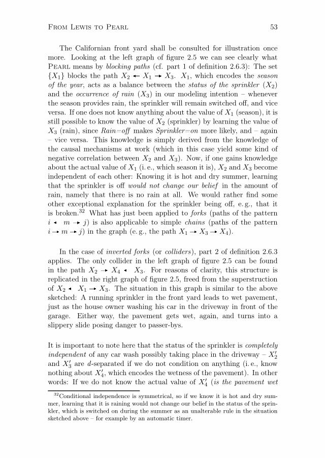
From Lewis to Pearl 53
The Californian front yard shall be consulted for illustration oncemore. Looking at the left graph of figure 2.5 we can see clearly whatPearl means by blocking paths (cf. part 1 of definition 2.6.3): The setX1 blocks the path X2 B X1 A X3. X1, which encodes the seasonof the year, acts as a balance between the status of the sprinkler (X2)and the occurrence of rain (X3) in our modeling intention – wheneverthe season provides rain, the sprinkler will remain switched off, and viceversa. If one does not know anything about the value of X1 (season), it isstill possible to know the value of X2 (sprinkler) by learning the value ofX3 (rain), since Rain=off makes Sprinkler=on more likely, and – again– vice versa. This knowledge is simply derived from the knowledge ofthe causal mechanisms at work (which in this case yield some kind ofnegative correlation between X2 and X3). Now, if one gains knowledgeabout the actual value of X1 (i. e., which season it is), X2 and X3 becomeindependent of each other: Knowing it is hot and dry summer, learningthat the sprinkler is off would not change our belief in the amount ofrain, namely that there is no rain at all. We would rather find someother exceptional explanation for the sprinkler being off, e. g., that itis broken.32 What has just been applied to forks (paths of the patterni B m A j) is also applicable to simple chains (paths of the patterniA mA j) in the graph (e. g., the path X1 A X3 A X4).
In the case of inverted forks (or colliders), part 2 of definition 2.6.3applies. The only collider in the left graph of figure 2.5 can be foundin the path X2 A X4 B X3. For reasons of clarity, this structure isreplicated in the right graph of figure 2.5, freed from the superstructionof X2 B X1 A X3. The situation in this graph is similar to the abovesketched: A running sprinkler in the front yard leads to wet pavement,just as the house owner washing his car in the driveway in front of thegarage. Either way, the pavement gets wet, again, and turns into aslippery slide posing danger to passer-bys.
It is important to note here that the status of the sprinkler is completelyindependent of any car wash possibly taking place in the driveway – X ′2and X ′3 are d-separated if we do not condition on anything (i. e., knownothing about X ′4, which encodes the wetness of the pavement). In otherwords: If we do not know the actual value of X ′4 (is the pavement wet
32Conditional independence is symmetrical, so if we know it is hot and dry sum-mer, learning that it is raining would not change our belief in the status of the sprin-kler, which is switched on during the summer as an unalterable rule in the situationsketched above – for example by an automatic timer.

54 From Lewis to Pearl
or not? ), learning the value of X ′3 (e. g., someone is washing the car infront of the garage) does not change our belief in X ′2 (the status of thesprinkler) or – to be a bit more precise – does not change our degreesof belief in the different possible values X ′2 can assume (expressed bythe unconditional probability distribution P (X ′2)). The missing edgebetween X ′2 and X ′3 is a consequence of our modeling intention: E. g.,the car owner would not switch off the sprinkler because he is washingthe car (maybe because he has put the sprinkler close to the drivewayand would not want himself to get sprinkled) – resulting in the absenceof the path X ′2 B X ′3. Neither does our modeling intention tell us thatthe status of the sprinkler somehow influences the decision of the houseowner to wash his car or not – resulting in the absence of the pathX ′2 A X ′3.Nevertheless, once we know the value of X ′4 (i. e., condition on the valueof X ′4), the variables X ′2 and X ′3 become conditionally dependent on eachother, and the path X ′2 A X ′4 B X ′3 is not d-separated any more. Inother words, once we know the value of X ′4, learning the value of X ′3would change our belief in the different possible values of X ′2 – and viceversa.
With his book Causality Judea Pearl is pleading for the use ofgraphs on the hunt for causal influences and efficient causes. He pro-motes those graphs as a mathematical means of precise notation in whichcomplex relationships can be presented compactly and easily accessiblyto the user of any discipline. In the second, extended edition of CausalityPearl emphasizes his standpoint in poetic manner:
As X-rays are to the surgeon,graphs are for causation.33
2.7 From modeling to model
A graph as in figure 2.5 together with explicit functional and determin-istic mechanisms exemplifies the analysis of situations as undertaken byeconomists, by sociologists, by epidemiologists, or diagnostic physicians.Joint probability distributions assigning degrees of belief (in Bayesianinterpretation) to any possible combination of atomic outcomes as dis-joint elementary events may serve as the basis for such a kind of study.A network may then be generated algorithmically to (graphically) dis-play all conditional dependencies, however, not necessarily uniquely in
33Cf. [Pearl 2009, p. 331].

From Lewis to Pearl 55
most cases. A characteristic momentum in the modeling phase is theembedding of natural causal assumptions which cannot be derived fromthe mere collection of data. These causal assumptions originate either inthe expertise of the modeler or in rather robust basic intuitions: Whenposing the question, in which direction to point an arrow between twonodes representing the age of a person and secondly her susceptibilityto a certain disease, we would prefer the arrow to be rooted in the agenode without much dispute. Obviously, this decision is grounded in quitebasal assumptions about stability and continuity of certain processes inour world.34
To extend the rather informal notion of modeling to the formal con-cept of model in the model-theoretic sense, I want to reproduce Pearl’sdefinition of a causal model at this point. It certainly has to go beyondthe concept of model in probability theory.35 There, a joint probabilityfunction over the variables under consideration yields a truth value forany proposition. E. g., the proposition “the probability for event A tooccur is greater than 1
2 ” is assigned the truth value 1 or 0 – dependingon the state of facts. Now, a causal model should be able to encodethe truth value of statements about causal relationships. This includessentences like
• “B occurred because of A,”
• “A may cause B,”
• “B will occur if we bring about A,”
• and counterfactual observations like “B would have been differentwere it not for A.”
Obviously, such statements cannot be evaluated in standard propo-sitional logic or any probability calculus, because they talk about – asJudea Pearl puts it – changes in the outer world and not about chang-ing convictions regarding a closed static world. Thus, causal models aremeant to provide information about possible external changes – they dothat by explicitly representing structural mechanisms, which are to bemodified through external alterations. More about that in the next step,but firstly on to the definition of a causal model.
34For this cf. Pearl’s analysis of Simpson’s Paradox in [Pearl 2009, pp. 177 f.].35For this and the following cf. [Pearl 2009, pp. 202 f.].

56 From Lewis to Pearl
Definition 2.7.1 (Pearl’s Causal Model)36
A causal model is a triple
M = 〈U, V, F 〉
where:
(i) U is a set of background variables (also called exogenous∗), thatare determined by factors outside the model;
(ii) V is a set V1, V2, . . . , Vn of variables, called endogenous, that aredetermined by variables in the model – that is, variables in U ∪ V ;and
(iii) F is a set of functions f1, f2, . . . , fn such that each fi is a map-ping from (the respective domains of) Ui∪PAi to Vi, where Ui ⊆ Uand PAi ⊆ V \Vi and the entire set F forms a mapping from U toV . In other words, each fi in
vi = fi(pai, ui), i = 1, . . . , n,
assigns a value to Vi that depends on (the values of) a select setof variables in V ∪ U , and the entire set F has a unique solutionV (u).∗∗,∗∗∗
Pearl’s respective footnotes shall be added for completeness in the fol-lowing:
* [2 in Pearl’s def.] We will try to refrain from using the term “exogenous”in referring to background conditions, because this term has acquired morerefined technical connotations [. . . ]. The term “predetermined” is used in theeconometric literature.
** [3 in Pearl’s def.] The choice of PAi (connoting parents) is not arbitrary, butexpresses the modeller’s understanding of which variables Nature must consultbefore deciding the value of Vi.
*** [4 in Pearl’s def.] Uniqueness is ensured in recursive (i. e., acyclic) systems.Halpern [Axiomatizing causal reasoning. In G. F. Cooper and S. Moral, edi-tors, Uncertainty in Artificial Intelligence, pages 202-210. Morgan Kaufmann,San Francisco, CA, 1998 ] allows multiple solutions in nonrecursive systems.
Pearl’s definition of a causal model, though formal and compact,comes with some loose ends, which are tightened in Appendix A (p. 137)by giving the formal mathematical definition of a random variable as
36Cf. def. 7.1.1 in [Pearl 2009, p. 203], footnotes given below with changed indexsymbols. Also see Pearl’s preliminary def. 2.2.2, [Pearl 2009, p. 44] where a causalmodel is defined as a pair M = 〈D,ΘD〉 consisting of a causal structure D (whichis a directed acyclic graph connecting a set of nodes V ) and a set of parameters ΘD
that specify the functional value assignment of each of the nodes in V .

From Lewis to Pearl 57
function of the outcome of a stochastic experiment. With these def-initions at hand, we may revisit Pearl’s definition of F , the set ofdeterministic mechanisms in the causal model. When looking at thesprinkler example, again, we can pick out one element of F , perhapsf4, which is associated with the variable X4 representing the answerto the question, if the pavement is wet or not. X4 is assigned itsvalue x4 by feeding the values of its parent variables (in the Marko-vian sense) along with the stochastic influence u4 into the correspond-ing function f4: X4 = f4(x2, x3, u4). Each variable, seen as a func-tion, has its own domain such that X4 is actually assigned its value byf4(X2(ω2),X3(ω3), U4(χ4)) with ω2 ∈ Ω2 = Dom(X2) = rain,no rain,ω3 ∈ Ω3 = Dom(X3) = sprinkler on, sprinkler off, and undescribedχ3 ∈ Dom(U3), which is not specified in any more detail. After all,any exogenous influence is an unmodeled influence, by choice of design– Dom(U3) might therefore contain plastic covers, burst water pipes,shattered coffee mugs, etc. For reasons of clarity, here and in the def-inition below we combine all potential exogenous influences on X4 intoone complex variable U4 (containing both positively contributing andpreventative external factors).37 Summing things up: The deterministicmechanisms fi take as arguments elements of the respective ranges ofthe parent variables (and the one complex exogenous variable), seen asfunctions.Part (iii) of definition 2.7.1 can now be supported with the followingformulation of causal mechanisms:
Definition 2.7.2 (Causal Mechanisms)38
F is a set of causal mechanisms for V , i. e., n functions f1, f2, . . . , fn(determining the value of each variable Vi in V ) such that
vi = fi(pai, ui)39
withF = fi | fi :
(
∏
k
Ran(PAik))
× Ran(Ui)→ Ran(Vi),
where 1 ≤ i ≤ |V | and for every i: 1 ≤ k ≤ |PAi|, Ui ∈ U (possiblycombining multiple contributing and/or preventing disturbance factorsinto one complex variable), and PAi ⊆ V \Vi. The entire set F formsa mapping from U to V with a unique solution.
37This is possible w. l. o. g., since all external factors satisfy the Markov property bydefinition, i. e., they are influencing the associated variables distinctly independently.
38The formulation given here is in agreement with the definition of the concept ofstructural model with deterministic functions in [Halpern & Pearl 2005a, p. 847].
39The boldface pai collects for each variable Vi the values of its parent variables.
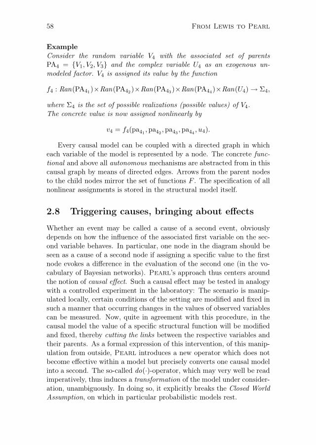
58 From Lewis to Pearl
ExampleConsider the random variable V4 with the associated set of parentsPA4 = V1, V2, V3 and the complex variable U4 as an exogenous un-modeled factor. V4 is assigned its value by the function
f4 : Ran(PA41)×Ran(PA42
)×Ran(PA43)×Ran(PA44
)×Ran(U4)→ Σ4,
where Σ4 is the set of possible realizations (possible values) of V4.The concrete value is now assigned nonlinearly by
v4 = f4(pa41,pa42
,pa43,pa44
, u4).
Every causal model can be coupled with a directed graph in whicheach variable of the model is represented by a node. The concrete func-tional and above all autonomous mechanisms are abstracted from in thiscausal graph by means of directed edges. Arrows from the parent nodesto the child nodes mirror the set of functions F . The specification of allnonlinear assignments is stored in the structural model itself.
2.8 Triggering causes, bringing about effects
Whether an event may be called a cause of a second event, obviouslydepends on how the influence of the associated first variable on the sec-ond variable behaves. In particular, one node in the diagram should beseen as a cause of a second node if assigning a specific value to the firstnode evokes a difference in the evaluation of the second one (in the vo-cabulary of Bayesian networks). Pearl’s approach thus centers aroundthe notion of causal effect. Such a causal effect may be tested in analogywith a controlled experiment in the laboratory: The scenario is manip-ulated locally, certain conditions of the setting are modified and fixed insuch a manner that occurring changes in the values of observed variablescan be measured. Now, quite in agreement with this procedure, in thecausal model the value of a specific structural function will be modifiedand fixed, thereby cutting the links between the respective variables andtheir parents. As a formal expression of this intervention, of this manip-ulation from outside, Pearl introduces a new operator which does notbecome effective within a model but precisely converts one causal modelinto a second. The so-called do(·)-operator, which may very well be readimperatively, thus induces a transformation of the model under consider-ation, unambiguously. In doing so, it explicitly breaks the Closed WorldAssumption, on which in particular probabilistic models rest.

From Lewis to Pearl 59
A causal effect can now be expressed as probabilistic quantity which maybe calculated from a probability distribution upon transformation:
Definition 2.8.1 (Pearl’s Causal Effect)40
Given two disjoint sets of variables, X and Y , the causal effect of X onY , denoted either as P (y | x) or as P (y | do(x)), is a function from X
to the space of probability distributions on Y . For each realization x ofX, P (y | x) gives the probability of Y = y induced by deleting from thestructural causal model all equations corresponding to variables in X andsubstituting X = x in the remaining equations.
This definition precisely expresses that the variable X does not dependfunctionally on any other variables any more. It will be assigned its valuefrom outside by an intervention external to the model. This process ofassigning is not encoded in the model itself, but is part of just such atransformation symbolized by the do(·)-operator.
Our Californian sprinkler example may be consulted for illustration,once more. The notion of external intervention becomes more transpar-ent if one sets out to examine the causal influence of the sprinkler on theslipperiness of the pavement: In our list of structural equations (2.10)the value of the random variable X2 is set to ‘switched on’, i. e., ‘true’.The corresponding equation thus becomes inoperative, and the value x2
in the equation for X4 will as well be fixed to ‘true’. Any possible alter-native for the value of X5 is eliminated – it shall be remarked here, thatis was certainly possible for X5 to assume alternative values before theintervention, i. e., ‘true’ or ‘false’. The unblocked causal flow from X2 toX5 now ultimately brings about the actual slipperiness of the pavement,of course modulo obstructive exogenous influences as plastic covers andsuch.
In the corresponding graph the modification of the structural equationsbecomes evident if for any variable the elimination of functional depen-dencies, graphically interpreted, means the elimination of influent edges.In the sprinkler example this means in particular that the transfer ofdegrees of personal belief between X1 and X2 becomes blocked. Beforethe intervention the modeling traces the mere observation of the setting.As soon as the running sprinkler is observed, one can infer with greatcertainty that is is summer or spring, due to the underlying positive cor-relation of X1 and X2. The dry seasons are finally responsible for thesprinkler being switched on, as was our modeling intention.
40Cf. def. 3.2.1 in [Pearl 2009, p. 70].
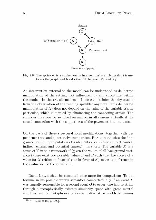
60 From Lewis to Pearl
X4
X2 X3
X1
X5
Season
do(Sprinkler = on) Rain
Pavement wet
Pavement slippery
Fig. 2.6: The sprinkler is “switched on by intervention” – applying do(·) trans-forms the graph and breaks the link between X1 and X2.
An intervention external to the model can be understood as deliberatemanipulation of the setting, not influenced by any conditions withinthe model. In the transformed model one cannot infer the dry seasonfrom the observation of the running sprinkler anymore. This deliberatemanipulation of X2 does not depend on the value of the variable X1, inparticular, which is marked by eliminating the connecting arrow: Thesprinkler may now be switched on and off in all seasons virtually if thecausal connection with the slipperiness of the pavement is to be tested.
On the basis of these structural local modifications, together with de-pendence tests and quantitative comparison, Pearl establishes the fine-grained formal representation of statements about causes, direct causes,indirect causes, and potential causes.41 In short: The variable X is acause of Y in this framework if (given the values of all background vari-ables) there exist two possible values x and x′ such that the choice of avalue for X (either in favor of x or in favor of x′) makes a difference inthe evaluation of the variable Y .
David Lewis shall be consulted once more for comparison: To de-termine in his possible worlds semantics counterfactually if an event Pwas causally responsible for a second event Q to occur, one had to stridethrough a metaphysically existent similarity space with great mentaleffort to test for metaphysically existent alternative worlds of various
41Cf. [Pearl 2009, p. 222].

From Lewis to Pearl 61
similarity distance, whether the statements ¬P and ¬Q describe the re-spective settings there correctly – or not. Even when restricting ourselvesto dichotomous variables, i. e., bivalent logic, respectively, depending onthe number of propositional constants we only obtain a semi-decidableprocedure for the identification of causes in the worst case, since we uni-versally quantify over possible worlds.
i
¬p
bbw
¬q?
P = p
Q = q
i
do(P = ¬p)
Q = ¬q?
w
Fig. 2.7: On the search for alternative testing environments for Q moving fromthe setting i to the setting w – as proposed by Lewis (on the left)and Pearl (on the right).
In direct comparison: When moving away from the actual world i
along the similarity relation in Lewis’ framework, we have to check inthe closest ¬p worlds w, if we also find ¬q to hold there. When model-ing generic relationships in the actual world i in Pearl’s formalism, weobtain a graph G mirroring the mere observation of correlations. Thetransition to an alternative world w where ¬p is to be determined canbe achieved qua intervention by means of the do(·)-operator: The vari-able P is set to ‘false’, influent edges are eliminated. The question isnow, whether the assignment of the P value also leads to a measurabledifference in the evaluation of the variable Q. If the causal effect of Pon Q in the model is identifiable (and Pearl gives algorithmic criteriafor determining if it is or not), then it can be calculated uniquely andefficiently on the basis of the stable functional mechanisms. Identify-ing causes in Pearl’s formalism can thus be understood both as naturaland operationally effective at the same time, because the invariant mech-anisms represent intuitively obvious basal assumptions, and because theexternal interventions are limited to local surgeries of the graph.

62 From Lewis to Pearl
2.9 Computing observational data for causal in-
ference
Making automated learning as efficient as possible is one of the chief goalsof computer scientists and has driven research in the field of artificial in-telligence. Several algorithms for inductive automated construction ofBayes nets from observational data have been developed and refined toachieve computational tractability. Typically, learning of Bayesian net-works is divided into two tasks: (i) learning of the underlying (graphical)structure of the net, i. e., its topology, and (ii) determining the condi-tional probabilities for each node (which can be represented in CPT’s –conditional probability tables).42
Causal inference is ultimately permitted by the stable skeleton of a causalmodel – its structure. Now, if we are given an arbitrary joint probabilitydistribution over a fixed set of variables V and want to derive directedarrows from raw data, we need to have some benchmark to be able tocompare different topologies with one another. The joint probabilitydistribution, understood as the vector of masses that are assigned toall different possible worlds (with size |V |2, in case all variables are di-chotomous), will serve as benchmark which each distribution induced bya Bayes net structure candidate can consequently be measured against.Different distance measures have been suggested for this task. The differ-ence between two joint probability vectors can be determined by usingthe Euclidian distance, thus summing up the squares of the distancesof all vector components, i. e., the weight differences between each twocorresponding possible worlds:
dE(x, y) =√
∑
i(xi − yi)2, (2.12)
where x, y are vectors (in our case, of masses of possible worlds). Alter-natively, the information-theoretic Kullback-Leibler divergence returnsthe weighted sum of the distances between the logarithms of each twocorresponding masses:
dKL(x, y) =∑
i
yi(log2 yi − log2 xi), (2.13)
again with the vectors x, y as above. Further refinements introduceweighting factors into the distance measure to, e. g., rank thinner net-works above denser ones in accordance with the demand for minimal
42Cf. for this and the following [Ertel 2009, pp. 219ff.].

From Lewis to Pearl 63
structures.43 Finally, creating an efficient algorithm for the search of thefittest Bayes net topology amounts to a minimization problem for whichgood heuristics are needed.
ExampleWolfgang Ertel considers the complete probabilistic model a meteorol-ogist might use to predict the amount of rainfall in the afternoon, solelyprojected from the weather conditions in the morning of the respectiveday.44
Sky Bar Rain P (Sky ,Bar ,Rain)
clear rising dry 0.40
clear rising rain 0.07
clear falling dry 0.08
clear falling rain 0.10
cloudy rising dry 0.09
cloudy rising rain 0.11
cloudy falling dry 0.03
cloudy falling rain 0.12
Table 2.1: The complete probabilistic model for the prediction of rainfall(Rain) in the afternoon, based on the weather conditions in themorning, if it is cloudy or clear (Sky), and whether the barometerrises or falls (Bar ).
Table 2.1 displays the masses of all eight possible worlds, combinatoriallylisting the joint probabilities for the sky (Sky) to be clear or cloudy, thebarometer (Bar) to rise or fall, and for rainfall (Rain) to occur or not.Since we want to compare vectors, the joint probability of the variablesSky, Bar , and Rain can now be presented as an 8-tuple:
P = 〈0.40, 0.07, 0.08, 0.10, 0.09, 0.11, 0.03, 0.12〉 (2.14)
Making this vector explicit now allows us to compare the following struc-tures with one another:
43Cf. e. g. [Ertel 2009, pp. 221 f.]; if N is the graphical structure of a Bayes netcandidate to be measured against some joint probability distribution P given in theform of vector of masses, then N is ranked by f(N) = size(N) + w · dKL(PN ,P),where PN is the joint probability distribution induced by the graph N , size(N) isthe number of entries in N ’s CPT’s, and w is some additional weighting factor thatneeds to be adjusted manually to balance the criteria of size and vector distance.
44Cf. [Ertel 2009, p. 175 and pp. 220 f.].

64 From Lewis to Pearl
(a) Sky A Rain B Bar and
(b) Sky A Bar A Rain,
with the corresponding joint probability vectors Pa,Pb. In the following,the computation of the distance between Pa and P shall be carried outin detail before Pa and Pb are compared in order to find the minimumdistance vector (with respect to P).
Step 1: Calculate the marginal probabilities. The a priori prob-abilities of the orphan variables Sky and Bar can be read off table 2.1directly by summing up the probabilities of equal variable assignments:P (Sky = clear) = 0.65 and P (Bar = rising) = 0.67. Of course, in thedichotomous case P (X = ¬x) is given by 1− P (X = x).
Step 2: Generate the CPT’s for all inner variables. This isdone by determining for each non-orphan variable X the ratio of each ofthe probabilities for X = x conditional on X’s parent variables, i. e., thevariables represented by its parent nodes in the graph. In the example thisis only the variable Rain, for which the following table can be calculated:
Sky Bar P (Rain = dry |Sky ,Bar )
clear rising 0.85
clear falling 0.44
cloudy rising 0.45
cloudy falling 0.2
Here, e. g., the first line is calculated from table 2.1 straightforwardly:
P (Rain = dry |Sky ,Bar ) (2.15)
=P (Rain = dry,Sky = clear,Bar = rising)
P (Sky = clear,Bar = rising)=
0.40
0.40 + 0.07= 0.85
Step 3: Generate the mass vector. In accordance with the ruleof iterated factorial decomposition (equation 2.5) and the independencecondition stated in the definition of Markovian parents (equation 2.8 indefinition 2.6.1), the mass vector induced by topology (a) can now be builtup by listing the masses of all possible worlds, generated combinatorially.

From Lewis to Pearl 65
E. g., the first entry is calculated as follows:
P (Sky = clear,Bar = rising,Rain = dry) (2.16)
= P (Rain = dry |Sky = clear,Bar = rising) ·
P (Sky = clear) · P (Bar = rising)
= 0.85 · 0.65 · 0.67 = 0.37
This is repeated analogously for all other possible worlds, finally resultingin the vector
Pa = 〈0.37, 0.065, 0.095, 0.12, 0.11, 0.13, 0.023, 0.092〉. (2.17)
Step 4: Measure the vector distance. Application of the measuresabove yields the distances
dE(Pa,P) = 0.0029 and
dKL(Pa,P) = 0.017.
Step 5: Find the minimum distance vector. The above steps didonly trace the procedure for Bayes net candidate (a). Of course, everyconceivable alternative structure should be treated analogously. If steps1–4 were to be performed for topology (b), the respective distances wouldbe
dE(Pb,P) = 0.014 and
dKL(Pb,P) = 0.09.
Since both measures mark Pa as the vector closer to P than Pb, Bayesnet structure (a) is considered to fit the data better than (b).45
Nevertheless, the task of finding the minimum distance vector facesproblems of complexity. The search space, i. e., the number of possibleDAG structures for a given set of variables V , super-exponentially growswith the number of variables |V |. Efficient and plausible heuristics areneeded to limit the search space before minimization is performed. Er-
tel suggests that one way of regaining computational tractability is to
45It is important to note that if an additional arrow Sky A Rain were to be insertedinto (b), thereby rendering the graph fully connected, the resulting graph (c) wouldyield distance dE(Pc,P) = 0, because in this uninformative presentation any twovariables are dependent.

66 From Lewis to Pearl
pick out those graphs that suit our basic causal assumptions, in the firstplace. If V1, . . . , Vn is a causal ordering of the variables in V , only thosegraphs would be considered that contain directed edges 〈Vi, Vj〉 withi < j.46 Since we precisely want to infer the set of potential causal struc-tures merely from raw observational data, the latter suggestion seems tocounteract our primary goals. Quite different from the metric approach,Thomas Verma and Judea Pearl constructively develop an algorithmfor the generation of marked patterns from stable probability distributions(over observed variables), i. e., classes of observationally equivalent latentstructures that are compatible with given data:
An autonomous intelligent system attempting to build a workablemodel of its environment cannot rely exclusively on preprogrammedcausal knowledge; rather it must be able to translate direct obser-vations to cause-and-effect relationships. However, given that sta-tistical analysis is driven by covariation, not causation, and as-suming that the bulk of human knowledge derives from passiveobservations, we must still identify the clues that prompt peopleto perceive causal relationships in the data. We must also find acomputational model that emulates this perception.47
In Pearl’s formulation of the algorithm for induced causation, re-ducing computational complexity through manual selection of poten-tial structural candidates (and perhaps erroneously dropping relevantgraphs) is traded for the task of (if only partly) directing the edges inthe limited set of graphs the algorithm finally returns.
Some notions must be clarified before the algorithm can be stated.What the algorithm will return is a class of observationally equivalent la-tent causal structures, i. e., a set of DAGs over observed and unobserved(latent) variables. Pearl adds the postulate of structure preference:One latent structure L is to be preferred to another one, L′, if and onlyif the observed part of the DAG of the latter can mimic the observedpart of the first. This amounts to saying that L should be favored ifby tweaking the precise specifications of all the functional mechanismsof L′ (represented by the edges in the graph of L′) the joint probabilitydistribution over the observed variables of L can be reproduced exactly.
46A causal ordering of the variables V1, . . . , Vn can be understood as satisfyingcertain constraints – e. g., if time is considered constitutive of causation, there cannotbe two variables Vi, Vj with i < j and Vj <temp Vi, where <temp indicates stricttemporal precedence.
47Cf. [Pearl 2009, p. 42].

From Lewis to Pearl 67
Succinctly, referring to the principle of Occams’s razor Pearl claimsthat “following standard norms of scientific induction, it is reasonable torule out any theory for which we find a simpler, less elaborate theorythat is equally consistent with the data [. . . ]. Theories that survive thatprocess are called minimal.”48 Consequently, minimality is defined rela-tive to a class L of latent structures such that a structure L is minimalwith respect to L if and only if there is no other structure L′ strictlypreferred to L.49 Then of course, as in the metric approach, the gen-erated structure must fit the data, i. e., it must be consistent with thegiven distribution P over the observed variables. In other words, for astructure L to be consistent with observational data P there must bea specification of the functional mechanisms in L that induces a jointprobability distribution (over all observed variables) equal to P .50 Withthese notions at hand we can explicate what inferred causation means:
Definition 2.9.1 (Pearl’s Inferred Causation)51
Given P , a variable C has a causal influence on variable E if and only ifthere exists a directed path from C to E in every minimal latent structureconsistent with P .
Pearl adds that he makes “no claims that this definition is guaranteedto always identify stable physical mechanisms in Nature. It identifies themechanisms we can plausibly infer from nonexperimental data; moreover,it guarantees that any alternative mechanism will be less trustworthythan the one inferred because the alternative would require more con-trived, hindsighted adjustment of parameters (i. e., functions) to fit thedata.”52
Nevertheless, theoretically we are not guaranteed that nonexperimen-tal data will always be minimal in the sense that it has only one uniqueminimal causal structure (modulo d-separation equivalence). The addi-tional assumption of stability tells us that given data P is usually highlyunlikely to hide probabilistic dependencies by precise cancelling. Stabil-ity thus implies that the list of independencies embedded in P remainsthe same even if the specification of individual functional mechanisms
48Cf. [Pearl 2009, p. 45].49As above, we definitely want to rule out the maximal case, i. e., the fully connected
graph that could mimic the behavior of any probabilistic model if the parameters(functional mechanisms) are tweaked the right way.
50Cf. [Pearl 2009, pp. 45 f.] for the precise definitions of latent structure, structurepreference, minimality, and consistency.
51Cf. [Pearl 2009, p. 46], definition 2.3.6.52Cf. [Pearl 2009, p. 47].

68 From Lewis to Pearl
changes.53 Of course, when we decide to allow for latent variables in thestructure, a stable input distribution P will not yield a unique minimalDAG, because – if not restricted by neighboring edges – the correlation oftwo variables can be due to either direct causal influence (either way) oran unknown common cause (a hidden, latent common parent variable).Accordingly, the IC* algorithm cumulatively enhances the structure tobe built up by adding individual arrowheads step by step (possibly re-turning bidirectional edges). The output of IC* is then a marked patternwith four types of edges (explained below), representing the class of ob-servationally equivalent minimal latent structures consistent with thedata.
Pearl’s IC* Algorithm(Inductive Causation with Latent Variables)54
Input: P , a stable distribution (with respect to some latent structure).Output: core(P ), a marked pattern.
1. For each pair of variables a and b, search for
a set Sab such that (a ⊥⊥ b |Sab) holds in P .
If there is no such Sab, place an undirected
link between the two variables a n b.
2. For each pair of nonadjacent variables a and b
with a common neighbor c, check if c ∈ Sab.
If it is, then continue .
If it is not , then add arrowheads pointing
at c (i.e., aA c B b).
3. In the partially directed graph that results ,
add (recursively) as many arrowheads as
possible , and mark as many edges as possible
according to the following two rules:
R1: For each pair of nonadjacent nodes a
and b with a common neighbor c, if the
link between a and c has an arrowhead
into c and if the link between c and b
has no arrowhead into c, then add an
arrowhead on the link between c and b
pointing at b and mark that link to
obtain c∗A b.
53Cf. [Pearl 2009, p. 48] for the definition of stability.54Cf. for this and the subsequently given characteristics of the resulting edges [Pearl
2009, pp. 52 f.].

From Lewis to Pearl 69
R2: if a and b are adjacent and there is
a directed path (composed strictly of
marked ∗-links) from a to b, then add an
arrowhead pointing toward b on the link
between a and b.
The resulting edges are divided into four groups:
1. a marked arrow a∗A b, signifying a directed path from a to b in
the underlying model (hinting at genuine causation);
2. an unmarked arrow aA b, signifying either a directed path from a
to b or a latent common cause aB L A b in the underlying model(thereby denoting potential causation);
3. a bidirected edge a BA b, signifying some latent common causeaB LA b in the underlying model (spurious association); and
4. an undirected edge a n b, standing for either a B b or a A b oraB LA b in the underlying model.
Rule R1 basically fixes the direction of an otherwise undirected edgeavoiding the introduction of an additional v-structure (which would im-ply an additional independence). Rule R2 fixes the direction of an oth-erwise undirected edge according to the requirement of acyclicity (whichwould be violated if the respective edge were oriented the other way).
a
b c
d
e
(a)
a
b c
d
e
(b)
a
b c
d
e
(c)
∗
a
b c
d
e
(d)
Fig. 2.8: Graph (a) displays the underlying actual structure encoded by a stableinput distribution P , (b) and (c) show the intermediate output of theIC* algorithm after working steps 1 and 2, finally resulting in (d)upon step 3.

70 From Lewis to Pearl
Figure 2.8 illustrates the working steps of the algorithm. Consider(a) to be the underlying actual structure of our nonexperimental dataP . (b) displays the intermediate output of the algorithm after step 1,(c) the introduction of v-structures in step 2, and (d) the output of IC*,a marked pattern with inserted arrowheads and starred links.
a
b c
d
e
(a)
a
b c
d
e
(b)
a
b c
d
e
(c)
a
b c
d
e
(d)
Fig. 2.9: The set of latent structures observationally equivalent to graph (2.8a),specifying the ambivalently marked edges of graph (2.8d).
Combinatorially spelling out the class of observationally equivalent la-tent structures amounts to drawing the four graphs depicted in figure2.9. These graphs all have the same v-structures in common, namely thesole one collider node bA dB c. Also, the directed link dA e is presentin each and every latent structure, introduced by virtue of rule R1 whichdirects edges in one way if the other direction were to introduce addi-tional v-structures into the graph (not derived from the independenciesin P ).55 The superstructure bn an c is then spelled out in all four pos-sible variants such that no new v-structure emerges.56 Now, to be ableto read the causal relation between two certain variables off the resultinggraph, some suitably chosen intervention variable Z must serve as hypo-thetical control knob – just as with structural manipulations, with theonly difference “that the variable Z, acting as a virtual control, must beidentified within the data itself, as if Nature had performed the experi-ment.”57
Pearl states that in this respect the IC* algorithm even leadsto the discovery of such control variables within the observational data.The notions of potential cause and genuine cause are accordingly definedwith respect to such control variables and moreover depend on the avail-
55The introduction of additional v-structures would generate additional indepen-dencies that are not in the data but could be read off the graph.
56Note that the double-headed arrow combinatorially cycles the upper diamondonce to produce the set of markov-equivalent structures in figure 2.9.
57Cf. [Pearl 2009, p. 54].

From Lewis to Pearl 71
able contexts encoded in the probability distributions, i. e., on how twotest variables X and Y behave if surrounding variables are conditionedon.
Definition 2.9.2 (Pearl’s Potential Cause)58
A variable X has a potential causal influence on another variable Y (thatis inferable from P ) if the following conditions hold.
1. X and Y are dependent in every context.
2. There exists a variable Z and a context S such that
(i) X and Z are independent given S (i. e., X ⊥⊥ Z |S) and
(ii) Z and Y are dependent given S (i. e., Z 6⊥⊥ Y |S).
In the sense of definition 2.9.2, variable b can be identified as a potentialcause of d in figure 2.8a if Z = c represents the virtual control variable(with respect to d) conditional on the context S = a. In other words,the putative cause variable and the hypothetical control variable must beindependent in some context – if a were missing altogether in the graph,it would even suffice to specify S = ∅. Nevertheless, b only qualifies as apotential cause of d, because – as displayed in figure 2.9 – the respectivelink between b and d can as well be realized as double-headed arrow,representing a possible common cause structure (e. g., as in figure 2.9a).Thus, b cannot be analyzed as being a genuine cause of d, i. e., as beinglinked to d by unambiguously directed edges, respectively.
Definition 2.9.3 (Pearl’s Genuine Cause)59
A variable X has a genuine causal influence on another variable Y ifthere exists a variable Z such that either:
1. X and Y are dependent in any context and there exists a contextS satisfying
(i) Z is a potential cause of X,
(ii) Z and Y are dependent given S (i. e., Z 6⊥⊥ Y |S), and
(iii) Z and Y are independent given S ∪X (i. e., Z ⊥⊥ Y |S ∪X);
or
2. X and Y are in the transitive closure of the relation defined incriterion 1.
58Cf. definition 2.7.1 in [Pearl 2009, p. 55].59Cf. definition 2.7.2 in [Pearl 2009, p. 55].
72 From Lewis to Pearl
In the sense of definition 2.9.3, variable d in figure 2.8a is analyzed asgenuinely causally influencing e. This time, we can take as control vari-able either of b, c, both being potential causes of d. No variables areneeded to fill the context: S = ∅. d and e are linked by a (if only one-link) chain of unambiguously directed edges. In a way, the test for theexistence of some control variable Z is utilized in both definitions aboveto determine the direction of the “causal flow,” just as what interventionsas structural manipulations are devised for. In case two variables X andY are dependent in some context (as a weakening of potential cause),but no direction of the causal relation can be made out by use of virtualcontrols, Pearl states one further definition: True spurious associationcan only be attributed to the existence of common causes.60
Now, in contrast with Ertel’s suggestion to pick out the graphs thatfit our causal intuitions before metrically computing some input distri-bution P , in Pearl’s approach the selection of potential working candi-dates amongst possible structures is put off till after P has been processedby IC*. The output class of observationally equivalent latent structuresmight be evaluated against the backdrop of expert causal knowledge orbasal everyday assumptions. Once the output class is restricted furtherand further, the marked pattern returned by IC* may be a helpful guidein designing possible test scenarios for the falsification of chosen arrowheads (through indication of potential further variables that could betaken into consideration, e. g., additional exogenous common causes).
2.10 About the identifiability of effects in causal
models
If a set of observational data (e. g., in the form of a joint probabilityfunction) is available to the empirically based causal analyst who wantsto evaluate the causal influence of one observed variable X on a distinctsecond, correlated variable Y , he is best advised to firstly exclude thatthe assessed correlation is actually induced by other factors than thepotential causal influence to be examined. So-called spurious correlationbetween X and Y is generated by confounding factors Z influencing bothX and Y at the same time, confounding our analysis, and ultimatelybiasing the estimate of the influence under consideration. This goesunder ‘confounding bias’ in the respective literature.61
60Cf. definition 2.7.3 (Spurious Association) in [Pearl 2009, pp. 55 f.].61Cf. for this and the following [Pearl 2009, pp. 182 f.].

From Lewis to Pearl 73
As an example from econometrics, consider Okun’s law which mapsthe relationship between unemployment and economic growth withinnational economy and postulates in compact manner linear dependence(which is one of the reasons for the law being so popular). Misinter-preting this dependence one might state: One necessary requirement fordecreasing unemployment is strong economic growth. Critics of Okun’slaw point to the fact that long-term variances of other parameters equallyimportant within national economy (as productivity, working time, joboffers) tend to significantly confound the direct relationship between theexamined quantities unemployment and economic growth. These addi-tional parameters, however, do not occur in the formulation of the law.To speak of cause, effect, causal relation, or causal influence in eitherdirection would certainly overstrain Okun’s law.
In his book Causality (2000/2009) Pearl makes out why the conceptof confounding goes largely unheeded in statistics course books:
As simple as this concept is, it has resisted formal treatment fordecades, and for good reason: The very notions of “effect” and “in-fluence” – relative to which “spurious association” must be defined– have resisted mathematical formulation. The empirical defini-tion of effect as an association that would prevail in a controlledrandomized experiment cannot easily be expressed in the standardlanguage of probability theory, because that theory deals with staticconditions and does not permit us to predict, even from a full spec-ification of a population density function, what relationships wouldprevail if conditions were to change – say, from observational tocontrolled studies. Such predictions require extra information inthe form of causal or counterfactual assumptions, which are notdiscernible from density functions [. . . ] 62
Density functions, i. e., probabilistic descriptions, precisely talk aboutclosed worlds and fixed environmental conditions, whereas in the frame-work of structural causal models the do(·)-operator serves as an effi-cient tool for the virtual inspection of dependencies in alternative testscenarios.
Now, as soon as the researcher – merely on the basis of given non-experimental and purely observational data – sets out to model a certainsituation, building a causal graph G and putting together the list of func-tional relationships renders it possible to examine, whether the causal
62Cf. [Pearl 2009, p. 183].

74 From Lewis to Pearl
influence of one factor X on another one, Y , can be uniquely estimated,at all – always, of course, within the scope of his modeling. Pearl
explicates the central idea behind this in his definition of identifiability :
Definition 2.10.1 (Pearl’s Identifiability of Causal Effects)63
The causal effect of X on Y is said to be identifiable if the quantityP (y | do(x)) can be computed uniquely from any positive distribution ofthe observed variables that is compatible with G.
Especially when there exist latent variables in the model potentiallycausally influencing both X and Y at the same time (if only indirectly),a quantitative estimate within the model must be adjusted by means ofother observed concomitant variables to exclude confounding bias andspurious correlation. How is a set of variables fit for this task to befound?
To efficiently accomplish the search for a suitable variable set, JudeaPearl formulates two criteria applicable again to the graph of a causalmodel. Making use of the so-called back-door and front-door criterionenables the researcher to easily identify from the diagram the set of nodesZ (of course representing the corresponding variables in the probabilitydistribution compatible with G) with which confounding influences canbe subtracted out. This adjustment is achieved by suitably summingup the potential values of all variables in Z. The two criteria shall bepresented in due brevity in the following:
Definition 2.10.2 (Pearl’s Back-Door Criterion)64
A set of nodes Z satisfies the back-door criterion relative to an orderedpair of nodes 〈Xi,Xj〉 in a DAG G if:
(i) no node in Z is a descendant of Xi; and
(ii) Z blocks every path between Xi and Xj that contains an arrowpointing towards Xi.
Analogously, Z satisfies the back-door criterion relative to two disjointsets of variables 〈X,Y 〉 if Z satisfies the back-door criterion relative toany pair 〈Xi,Xj〉 with Xi ∈ X and Xj ∈ Y .
63Cf. definition 4 in [Pearl 1995, p. 674], slightly adjusted here to maintain consis-tent notation.
64Definition 3.3.1 in [Pearl 2009, p. 79].

From Lewis to Pearl 75
Such a set Z accordingly d-separates all paths that would leave open aback-door into Xi for some possible confounding factor – hence the nameof the criterion. In the miniature example given in the left graph of figure2.10 the direct influence of variable Xi on variable Xj shall be assessed– obviously along the path Xi A X6 A Xj . Employing the d-separationcriterion, potential confounders outside the path Xi A X6 A Xj can bemade out, i. e., variables that – within the causal diagram – influenceboth Xi and Xj simultaneously when wiggled qua modification. Theback-door criterion now identifies the minimal sets X3,X4, or X4,X5alternatively, as sufficient for screening off spurious influences. X4 alonewould not do the job, because although – according to the definitionof the d-separation criterion – the path Xi B X4 A Xj would becomeblocked by conditioning on X4, quite on the contrary X4 opens the flowof information along the outer path via X1 and X2 as the collider nodein this v-structure.
X1
X2
X3
X4
X5
X6
Xi
Xj
U (Unobserved)
Xi XjZ
Fig. 2.10: In the left diagram the effect of Xi on Xj can be estimated con-sistently by means of adjusting for the variable pairs X3, X4 orX4, X5; the right diagram illustrates adjustment for Z by apply-ing the front-door criterion.
Now, the front-door criterion takes care of those cases in which pos-sible back-door paths run through unobserved variables, which are ofcourse not apt for being a candidate set Z possibly screening off spuri-ous correlation in computation – unobserved variables cannot be adjustedfor. Pearl’s graphical solution:
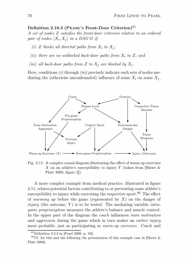
76 From Lewis to Pearl
Definition 2.10.3 (Pearl’s Front-Door Criterion)65
A set of nodes Z satisfies the front-door criterion relative to an orderedpair of nodes 〈Xi,Xj〉 in a DAG G if:
(i) Z blocks all directed paths from Xi to Xj ;
(ii) there are no unblocked back-door paths from Xi to Z; and
(iii) all back-door paths from Z to Xj are blocked by Xi.
Here, conditions (i) through (iii) precisely indicate such sets of nodes me-diating the (otherwise unconfounded) influence of some Xi on some Xj .
Warm-up Exercises (X) Intra-game Proprioception Injury (Outcome)
Team Motivation,Aggression
NeuromuscularFatigue
Contact Sport
TissueWeaknessPrevious
Injury
Pre-gameProprioception
Fitness Level Connective TissueDisorder
Coach Genetics
Fig. 2.11: A complex causal diagram illustrating the effect of warm-up exercisesX on an athlete’s susceptibility to injury Y (taken from [Shrier &Platt 2008, figure 2]).
A more complex example from medical practice, illustrated in figure2.11, relates potential factors contributing to or preventing some athlete’ssusceptibility to injury while exercising the respective sport.66 The effectof warming up before the game (represented by X) on the danger ofinjury (the outcome, Y ) is to be tested. The mediating variable intra-game proprioception measures the athlete’s balance and muscle control.In the upper part of the diagram the coach influences team motivationand aggression during the game which in turn makes an earlier injurymore probable, just as participating in warm-up exercises. Coach and
65Definition 3.3.3 in [Pearl 2009, p. 82].66Cf. for this and the following the presentation of this example case in [Shrier &
Platt 2008].

From Lewis to Pearl 77
genetic predisposition together contribute to the athlete’s fitness level,and so forth. The question (in the center of the graph), if the respectivegame falls under the category of contact sport or not, also influences theprobability of a previous injury independently of team motivation.
The influence of warm-up exercises on potential injury is obviously con-founded by a multitude of factors. Application of the back-door crite-rion facilitates the search for a set of nodes Z which helps adjustingconfounding factors: Those variables measuring neuromuscular fatigueand possible tissue weakness are jointly sufficient for screening off spuri-ous influences because they intercept all back-door paths from X to theputative outcome Y . The path running through the question, if contactsport or not, is inactive without conditioning anyways, since it containsa collider node – an inverted fork. Previous injury is thus to be excludedfrom the adjusting set of variables Z, because gaining knowledge aboutprevious injuries precisely opens a back-door again, thereby establish-ing indirect dependence between warm-up exercises and susceptibility toinjury. Pearl’s graphical criteria facilitate the identification of con-founders and adjusting variables even in this rather complex examplefrom medical practice.
Now, in case the effect of some variable on a second variable turnsout to be identifiable in a given causal model, Pearl offers a set ofrules, sound and complete, for the reduction of probabilistic expressionscontaining the do(·)-operator to expressions without it. The so-calleddo-calculus enables the researcher to estimate post-intervention quanti-ties merely from non-experimental, observational distributions. For thecase that a set of variables screening off some causal flow from spuriousinfluences can be made out – either by employing the back-door criterionor the front-door criterion – Pearl moreover presents two formulae foradjustment in [Pearl 1995], also restated in [Pearl 2009, pp. 79 ff.]. Thefollowing two respective theorems shall be given for the sake of complete-ness and conclude this section before the concept of token causation willbe examined more closely below:
Theorem 2.10.4 (Pearl’s Back-Door Adjustment)67
If a set of variables Z satisfies the back-door criterion relative to 〈X,Y 〉,then the causal effect of X on Y is identifiable and is given by the formula
P (y | do(x)) =∑
z
P (y |x, z)P (z). (2.18)
67Theorem 3.3.2 in [Pearl 2009, pp. 79 f.].

78 From Lewis to Pearl
Theorem 2.10.5 (Pearl’s Front-Door Adjustment)68
If a set of variables Z satisfies the front-door criterion relative to 〈X,Y 〉and if P (x, z) > 0, then the causal effect of X on Y is identifiable andis given by the formula
P (y | do(x)) =∑
z
P (z |x)∑
x′
P (y |x′, z)P (x′). (2.19)
2.11 Singular causation and the actual cause
To let the protagonists of this discussion appear once more on stagetogether, or to at least present their approaches in a certain concord,we take up the notion of singular causation as discussed by Pearl inCausality. So we are not talking about generic analysis as in “rain causesthe street to get wet,” but deal with situations on token level. As an ex-ample we look at the administering of some medication in a controlledclinical study.69 When evaluating the collected data statically, it turnsout that the medication neither affects the recovery of the patients posi-tively nor negatively – on average. Furthermore, we pick out one specificpatient who was administered the medication and fully recovered subse-quently. Now, a causal model ought to be able to answer in particular,whether the patient’s recovery occurred due to the treatment, despitethe treatment, or completely regardlessly of the treatment. An answercannot be given if only observational data is available, since the patientwas never tested without administering the medication – probabilitiesunder deviant conditions cannot be compared.
Pearl points out clearly that in such cases on token level the solutionlies solely in the counterfactual analysis of the problem: “What wouldthe probability of recovery have been if the medication had not beenadministered?” This counterfactual formulation precisely implies thedeviation from observed data. The desired value can be calculated froman alternative model in which the counterfactual antecedent is virtuallyforced to be true. This very task is achieved by the do(·)-operator instructural causal models.
To give an example: We want to learn if the intervention ¬p would havebrought about ¬q if in fact we already know that both p as well as q have
68Theorem 3.3.4 in [Pearl 2009, p. 83].69This example is taken from [Pearl 2009, pp. 33 f.].

From Lewis to Pearl 79
occurred factually. The effect of an intervention can indeed be identifiedcontra and moreover post factum in the methodological triple jump alongthe lines of natural reasoning:70
1. Abduction: Having observed p and q, i. e., our factual evidence,we infer the explanation (i. e., a hypothesis or a state of the world)going backwards (or upwards) in the network.
2. Action: In the context of this fixed environment we perform thelocal surgery ¬p by intervening in the structural model (therebytransforming the graph).
3. Prediction: The autonomous mechanisms of the structural causalmodel now allow for predicting the value assignment of Q (if thecausal effect of P on Q is identifiable, at all).
Performing steps 1 through 3 basically amounts to traversing the causalnetwork twice – once upwards to determine the values of all exogenousvariables and then downwards again after transforming the network byclipping all arrows pointing towards P (thereby lifting P from the in-fluence of its direct causes). Letting the context information propagatethrough the network again, we are ultimately able to read off the graphthe counterfactually predicted value of Q.71
The scheme above unifies the essential features of Pearl’s agendaonce more, which are conceptually and methodologically sorted out againby Christopher Hitchcock, who writes in his article Causal Modellingin the Oxford Handbook of Causation :
There is an important pragmatic difference between counterfactualsand interventions: we are typically interested in knowing the truthvalues of counterfactuals after the fact, whereas we are usuallyinterested in evaluating the consequences of potential interventionsbefore they are carried out.72
Interventions by use of the do(·)-operator precisely allow for such hypo-thetical tests in virtual, alternative experimental designs. But, if the
70Cf. for this and the following [Pearl 2009, p. 37 and pp. 205 ff.].71This procedure is presented by Pearl in twin networks, where going upwards
and (after transforming the model) going downwards through the same graph is in-terpreted as stepping sideways into the almost identical copy of the original graphwhere all edges directed into Q are clipped.
72Cf. [Hitchcock 2009a, p. 303].
80 From Lewis to Pearl
do(·)-operator, in externally bringing about Lewis’ “small miracles,”stands in close methodological vicinity to Lewis’ similarity relation, andif Pearl accuses Lewis of circularly taking some immanent notion ofcausation for granted when comparing two worlds with respect to theirsimilarity to a third, must Pearl not defend himself against his ownallegations, as well? – Does he not also analyze complex causal relation-ships by evaluating basal natural assumptions, which themselves conveycausal meaning, and do so necessarily, as Pearl stresses? I would liketo give the floor to Pearl himself, who formulates the following in the2005 paper Causes and Explanations together with collaborator JosephHalpern:
It may seem strange that we are trying to understand causalityusing causal models, which clearly already encode causal relation-ships. Our reasoning is not circular. Our aim is not to reducecausation to noncausal concepts but to interpret questions aboutcauses of specific events in fully specified scenarios in terms ofgeneric causal knowledge such as what we obtain from the equa-tions of physics. The causal models encode background knowledgeabout the tendency of certain event types to cause other event types(such as the fact that lightning can cause forest fires). We use themodels to determine the causes of single (or token) events, suchas whether it was arson that caused the fire of 10 June 2000, givenwhat is known or assumed about that particular fire.73
Grounding causal analysis in such basal causal assumptions can in thethus explicated sense rightfully be called fruitful because it admits uti-lizing the introduced notions and methods constructively. Certainly,emphasizing truly deterministic causal mechanisms much rather bringsacuteness into causal analysis than drawing the researcher over the no-tional fringes of naughtiness.
Utilizing our understanding of the mechanisms at work to learn abouthypothetical alternative situations is one direction of posing questionsabout token causation – we might also look the other way and employthe specification of a causal model to learn which of the actually observedoccurrences is the true cause of another distinct observed event. In otherwords: How can we find out, if some realized putative cause candidate isindeed responsible for having brought about some observed other event,maybe even post factum? To be able to deal with this sort of token (orsingular) causal reasoning, Pearl advances in two steps: Firstly, our
73Cf. [Halpern & Pearl 2005a, p. 849].

From Lewis to Pearl 81
understanding of the situation, i. e., the parameterization of the model(or the specification of the functional deterministic mechanisms), is cou-pled with some fixed context – the given (vector of) circumstances #„u .Secondly, by ultimately quantifying over possible value assignments tosubsets of the observed variables in V an active causal process is carvedout, thereby marking the minimal set of contributory causes
#„
X of thetoken event Y = y under consideration, in a sense in virtual comparisonwith different configurations of the model – different qua intervention.
#„
U
# „
W
#„
X
#„
Z
Y
V
Fig. 2.12: The idea behind Pearl’s definition of the actual cause, illustrated asrelations between subnets of the causal model M .
#„
U = #„u indicatesthe obtaining circumstances, the observed variables are partitionedsuch that V =
# „
W ∪#„
Z with#„
Z signifying the active causal processrelating
#„
X = #„x and Y = y, where#„
X ∪ Y ⊆#„
Z .
Figure 2.12 illustrates the idea behind Pearl’s definition of the ac-tual cause (definition 2.11.1 below), relating subnets of the causal modelin Venn-like presentation: The variables in the causal model M are as-signed their values according to some specification of the context
#„
U = #„u .The tuple 〈M, #„u 〉 especially induces the unique assignment of values tothe n-ary vector
#„
X, the total cause, aggregating all variables X1, . . . ,Xn
as contributory causes of the event Y = y. Finally, the vector#„
Z (as-suming the corresponding observed values
#„
z∗) can be understood as theactive causal process in M under the obtaining circumstances #„u . It turnsout that the definition of
#„
Z picks out (in addition to#„
X and Y ) just thevariables mediating between
#„
X and Y on the paths directed from thevariables in
#„
X to Y .74
74Cf. Pearl’s remarks in [Halpern & Pearl 2005a, p. 854].

82 From Lewis to Pearl
Definition 2.11.1 (Pearl’s Actual Cause)75
#„
X = #„x is an actual cause of Y = y in 〈M, #„u 〉 if the following threeconditions hold:
1. 〈M, #„u 〉 (#„
X = #„x ) k (Y = y), that is, both#„
X = #„x and Y = y aretrue in the actual world.
2. There exists a partition #„
Z,# „
W of V with#„
X ⊆#„
Z and some setting#„
x′ and#„
w′ of the variables in#„
X and# „
W such that if the fixed context#„u induces the value assignment
#„
z∗ for the variables in#„
Z , i. e., if〈M, #„u 〉 (
#„
Z =#„
z∗), then both of the following conditions hold:
(a) The intervention 〈#„
X,# „
W 〉 ← 〈#„
x′,#„
w′〉 (assigning non-actualvalues to
#„
X and# „
W ) changes Y = y from true to false inthe model, i. e., 〈M, #„u 〉 6 (Y = y) (in the accordingly trans-formed model).76
(b) 〈M, #„u 〉 (Y = y) under any possible interventional assign-
ment 〈# „
W ′,# „
Z ′〉 ← 〈#„
w′,#„
z∗〉 for all subsets# „
W ′ of# „
W and all
subsets# „
Z ′ of#„
Z , as long as#„
X is kept at its current value #„x ,i. e.,
#„
X ← #„x ; in other words, setting any subset of variablesin
# „
W to their values in#„
w′ should have no effect on Y , as longas
#„
X is kept at its current value #„x , even if all the variablesin an arbitrary subset of
#„
Z are set to their original values inthe context #„u .
3.#„
X is minimal, i. e., no subset of#„
X satisfies conditions 1 and 2.77
In the definition of the actual cause, condition 1 simply says that weare dealing with token causation – cause and effect actually occur in thecausal model M (with a full specification of the functional mechanisms)if the context #„u is given. Section 2 of the definition postulates a parti-tioning of the observed variables V into those variables (
#„
Z) involved inthe causal process connecting
#„
X to Y and those variables (# „
W ) irrelevant
75Cf. Pearl’s presentation in [Halpern & Pearl 2005a, p. 853] (definition 3.1 andrefinements in sect. 5) and Spohn’s discussion thereof in [Spohn 2010, sect. 2]; theformulation given here differs slightly from Pearl’s to maintain consistency withpreviously introduced conventions.
76The notation p#„
X ← #„xq symbolizes the transformation of the model by iterativeapplication of the do(·)-operator (as introduced above) for each variable in the n-ary vector
#„
X , thereby pruning the respective graph of the model and modifying allstructural equations in accordance with do(X1 = x1), do(X2 = x2), . . . , do(Xn = xn).
77As Pearl adds: “Minimality ensures that only those elements of the conjunction#„
X = #„x that are essential for changing Y = y in 2(a) are considered part of the cause;inessential elements are pruned.” – cf. [Halpern & Pearl 2005a, p. 853].

From Lewis to Pearl 83
for the observed effect Y . Condition 2(a) says that changing the valuesof
#„
X also renders the event Y = y inactive. Condition 2(a) also allowsfor changing the values of
# „
W (the variables seen as irrelevant for bring-ing about Y = y), since they might sustain the effect, thereby maskingthe influence of
#„
X on Y which we are after. On the other hand, it is tobe excluded that only the assignment of #„w to
# „
W is responsible for theevent Y = y, so condition 2(b) tightens things again by postulating thatonly the actual observed values of
#„
X succeed in bringing about the effectY = y: Arbitrary subsets of the irrelevant variables in
# „
W may assumearbitrary non-actual values
#„
w′. Y = y will still be observed if only#„
X isset to its actual observed value #„x . Pearl points out that setting
#„
X to#„x necessarily entails the assignment
#„
Z =#„
z∗, since#„
Z contains the veryvariables mediating between
#„
X and Y – the active causal process.
It is important to note one thing here: If our causal model at handis narrow in the sense that it only consists of the active causal processalone, the analysis is done without hassle – no ambiguities arise. Forexample, if the model is a simple chain, then the (total) cause of someevent Y = y is simply the variable X corresponding to the single par-ent node of Y , which is minimal in the sense of condition 3 above. If,nevertheless, the model is enriched arbitrarily by adding supposedly ir-relevant information (about potential causal relations), things might getmuddled. This especially shows in cases of causation by omission wheresome effect is produced by some specific event not being realized, andwhere it is this specific event that the researcher wants to single out andtest for potential causation and not any other potential cause candidatesthat did not get realized either. Consider the following example, takenfrom [Halpern & Pearl 2005a, p. 871 (example 5.3)] (referring to anunpublished text by Hall and Paul):
Suppose Suzy goes away on vacation, leaving her favorite plant inthe hands of Billy, who has promised to water it. Billy fails todo so. The plant dies – but would not have, had Billy watered it.. . .Billy’s failure to water the plant caused its death. But VladimirPutin also failed to water Suzy’s plant. And, had he done so, itwould not have died. Why do we also not count his omission as acause of the plant’s death?
Halpern and Pearl make two suggestions: (i) Slim down the modeland do away with the endogenous variable Putin.waters.the.plant. Thiswould leave the analyst with only Billy’s failure as potential cause can-didate. (ii) If the richer structure is to be preserved, do not check all

84 From Lewis to Pearl
variable assignments for the putatively irrelevant variable set# „
W . For-mally this amounts to defining extended causal models by adding setsof allowable settings E of the endogenous variables. In the case of theabove example, our modeling intuition tells us that the variable settingPutin.waters.the.plant = 1 is to be excluded from the respective set ofallowable settings E . That is, we are not considering Putin’s failure towater the plant as true cause, as relevant for the situation, as informa-tive when mentioned in discussion, etc. Both strategies are of pragmaticnature but necessary if Pearl’s causal analysis is to be implemented es-pecially in contexts where (neglected) responsibility is to be determinedor guilt is to be assessed. It seems as if Pearl were loosening his ownrigorous framework at this point again. But he answers:
Are we giving ourselves too much flexibility here? We believe not.It is up to a modeler to defend her choice of model. A modelwhich does not allow us to consider Putin watering the plant canbe defended in the obvious way: that it is a scenario too ridiculousto consider.78
Ultimately – and summing up Pearl’s explications – this means thatthe task of discerning causes (especially singular ones for explanatorypurposes) comes down to enriching bare structures by adding non-causalknowledge and to model-relatively querying lower-level basal relationsupon limiting possible settings (i. e., upon marking worlds to consider).These facets will be picked up again, exploited, and expanded further inchapter 3 now.
78Cf. [Halpern & Pearl 2005a, p. 871].

Chapter 3
Causality as epistemicprinciple of knowledgeorganization
as [resemblance, contiguity,causation] are the only ties ofour thoughts, they are really tous the cement of the universe
David Hume, An Abstract of a“Treatise of Human Nature”
When Judea Pearl takes a stand on the ontic (metaphysical) statusof causation in his book Causality, he clearly localizes causal relationshipson the objective (physical) side of the pair ontological versus epistemic(doxastic):1
[. . . ] causal relationships are ontological, describing objective phys-ical constraints in our world, whereas probabilistic relationshipsare epistemic, reflecting what we know or believe about the world.Therefore, causal relationships should remain unaltered as long asno change has taken place in the environment, even when ourknowledge about the environment undergoes changes.2
Nevertheless, as becomes obvious from his comments on possible, allow-able settings of the variables in the causal model at hand (or on ways of
1Compare chapter 1, sect. 1.9, for a list of decisions to take in the process ofdevising a theory of causation.
2Cf. [Pearl 2009, p. 25].

86 Causality as epistemic principle
slimming down causal models), it is the modeler’s choice which comes be-fore the assessment of causes and their effects (within the chosen frame):Causal inference remains model-relative in Pearl’s framework, after all.Still, the holistic and monolithic path followed by an account of causa-tion on the basis of hypothetical, possible interventions seems (i) to bevery attractive to various (at least empirical) disciplines that build uponthe practice of experimentation and (ii) to correspond very well with ourintuitions, summed up in the observation – or rather in the postulate –“wiggling the cause affects the effect – and not vice versa.” But on whatontological grounds can this claim be understood and made exploitablefruitfully, if a purely physically objective interpretation faces criticism?
3.1 The total system and the modality of inter-
ventions
One way of answering the question, where causation is to be localizedmetaphysically, is to simply deny the existence of such a relation, asBertrand Russell does in his often-quoted seminal inquiry On the No-tion of Cause (1913):
[. . . ] the reason why physics has ceased to look for causes is that, infact, there are no such things. The law of causality, I believe, likemuch that passes muster among philosophers, is a relic of a bygoneage, surviving, like the monarchy, only because it is erroneouslysupposed to do no harm.3
Examining what we mean by saying that one event causes a second event,Russell finds that mature science has withdrawn from the business ofmarking off suitable events and has rather settled on specifying variablesand their corresponding measurement methods for the analysis of func-tional dependencies instead of causal relations.4 Russell must arriveat his concluding judgment – he bases his argument on the existence ofactual events and physical processes. The analysis of everyday language
3Cf. [Russell 1913, p. 1].4Cf. for this and the following [Dowe 2009, pp 214 f.]. There (p. 215), Phil Dowe
briefly comments on this finding:
Russell simply makes the point that [science] focuses on functional rela-tions between variables, a focus far removed from the kind of common-sense events that we take to be causes and effects.
Quite contrary to that, Pearl in his framework introduces events as random variablesand causal relations as deterministic functional relations between those variables,aiming at a close connection with intuitive reasoning.

Causality as epistemic principle 87
with widely defined events (stated by expressions such as ‘some person’shitting the billiard ball’) ultimately yields the result that there are noreal regular causes, since any event can be intercepted by way of excep-tion and rendered void in its bringing about the effect (in this case, thebilliard ball falling in some pocket) – there can always be unmentionedfurther preventative circumstances complicating our attribution of causalefficacy. On the other hand, going narrow trivially eliminates the con-cept of cause, too, as Russell argues. As soon as any cause-effect pairof events is described in all its pertaining details, saying that one eventcauses the other becomes trivially true, since this case of regularity onlyhas one instance. Talk of causation can thus be exchanged for talk ofdetermination without losing any inherent meaning.
Now, if one wants to stick to the Bayes net account of determinis-tic causation with interventions (going from types to tokens), there isno other option than to agree with Lord Russell: Any causal modelin Pearl’s sense relies on an agreement about the context, i. e., onthe choice of variables that are to be excluded from modeling as ceterisparibus conditions. Violation of one of these silent (in principle infinitelymany) conditions may render the whole model useless. As a consequence,no causal model thus construed will suffice to hold for all thinkable casesof application – for any causal model there is always a model closer to ob-jective physical reality (by outward augmentation or zooming in).5 Onthe other hand, strengthening the narrow description of events wouldultimately result in infinitely narrow, point-like instantiations of certainfeatures (following Kim’s explication) such that the full Bayes net thusconceived would become infinitely dense, ultimately losing its propertyof being a network altogether, thus not being modifiable by structural lo-cal surgeries in Pearl’s sense for testing causal directionality anymore.6
J. L. Mackie arrives at a similar conclusion in his examination of causalpriority.7 Basing his argumentation on the ontological interpretation ofcausation he admits that, if one assumes total determinism, there is noway to find out about the direction of causation anymore – any specificevent is apt for the explanation (or prediction) of any other event, since
5To avoid entering any vicious circle here, closer simply means taking more eventsinto account – in a way, fine-graining the model.
6This remark basically combines both points made by Russell: Going narrowand storing all potentially relevant information in the model amounts to storingall information in the model (in dense arrangement). Consequently, what NancyCartwright in [Cartwright 2001, sect. 3a] calls “God’s big Bayes net” in referenceto what Wolfgang Spohn in [Spohn 2000, p. 11] calls the “all-embracive Bayesiannet” cannot be a net structure anymore.
7Cf. for this and the following [Mackie 1980, pp. 189 ff.].

88 Causality as epistemic principle
any two events in this system (or realizations of two distinct variables,respectively) are related in strict manner:
If you have too much causation, it destroys one of its own mostcharacteristic features. Every event is equally fixed from eternitywith every other, and there is no room left for any preferred direc-tion of causing.8
Moreover, assuming total determinism in the total system (alongwith Laplace, Einstein, or modern deterministic interpretations ofquantum mechanics) finally makes Pearl’s interventionist account ofcausation inapplicable altogether. If there is nothing external to thesystem anymore, even the possibility of thinking external interventionsbecomes inaccessible if those manipulations are to have any meaningat all (perhaps some counterpart in some possible world – to stay inthe laboratory picture; but alternative possible worlds would have to becompletely incompatible and incomparable with the actual world at alltimes, since Lewis’ “small miracles” are excluded if total determinism ispostulated).
Does the hunt for causes stop here? Russell judges that the law ofcausality is only erroneously supposed to do no harm – he must admit,after all, that causal talk obviously does convey meaning. Pursuing tocarve out the unifying content might thus still turn out to be fruitful inthe end.
3.2 Subnets for epistemic subjects
When Wolfgang Spohn ponders the metaphysical status of causal depen-dence, he finally arrives at the conclusion (also heading his paper from2000) that “Bayesian Nets Are All There Is To Causal Dependence”:
So far, I have only introduced two distinct graph-theoretical rep-resentations: one of causal dependence between variables and oneof conditional probabilistic dependence. However, the core observa-tion of each probabilistic theory of causation is that there is a close
8Cf. [Mackie 1980, p. 191]. Note that Mackie puts forward a variant of aninterventionist (or at least agentive) account of causation. He makes this explicitwith his first rendition of causal priority in [Mackie 1980, p. 190]:
A first approximation to an analysis of ‘X was causally prior to Y ’, whereX and Y are individual events, is ‘It would have been possible for an agentto prevent Y by (directly or indirectly) preventing, or failing to bring aboutor to do, X’ [. . . ].

Causality as epistemic principle 89
connection between causal and probabilistic dependence, that thetwo representations indeed coincide, i.e. that each causal graph isa Bayesian net. Thereby, the Markov and the minimality conditionturn into the causal Markov and the causal minimality condition.9
As in Pearl’s framework sketched above, some variable’s Markovianparents can consequently be interpreted as the direct causes of the eventrepresented by this variable. Spohn goes on by exploiting this:
[D]irect causal dependence is obviously frame-relative [. . . ]. Therelativization would be acceptable, if it concerned only the direct/indirect distinction: what appears to be a direct causal dependencywithin a coarse-grained frame may well unfold into a longer causalchain within a more fine-grained frame. [. . . ] It’s worse, however.The whole notion of causal dependence is frame-relative accordingto [its] definition: where there appears to be a direct or an indi-rect causal dependency within a coarse-grained frame, there maybe none within a more fine-grained frame, and vice versa.10
An answer to the question what guidelines we have for building netstructures of causal models that truly reflect ‘real causation’ might notbe feasible, after all, Spohn concedes:
In the final analysis it is the all-embracive Bayesian net repre-senting the whole of reality which decides about how the causaldependencies actually are. Of course, we are bound to have only apartial group of this all-embracive Bayesian net.11
If this seems to be a necessary shortcoming of representing causal de-pendencies in suitably confined Bayesian nets, why not understand itas an essential feature of causal reasoning in the first place? The in-terventionist account of causation even requires the net structures ofcausal models to correspond to subsystems of the total system – expertknowledge or common sense tells us how to carve out sufficiently openand at the same time sufficiently closed subnets of our (directly or indi-rectly) perceived surroundings. Open to allow for hypothetical externalinterventions and closed to mark off the variables under considerationfrom those assigned merely exceptional influence as in the laboratorypicture.12 Deciding upon the set of variables considered illuminating for
9Cf. [Spohn 2000, p. 5].10Cf. [Spohn 2000, p. 7].11Cf. [Spohn 2000, p. 11]. Also see footnote 6 of this chapter for a critical remark
on the term ‘all-embracive Bayesian net.’12Judea Pearl comments on the origins and ramifications of breaking the ‘closed
world assumption’ in greater depth in sect. 7.5 of [Pearl 2009].

90 Causality as epistemic principle
the analysis to be conducted is obviously a subjective (sometimes highlypragmatic) process that may differ from one epistemic agent to the nexteven if performed in compliance with rational standards. The struc-ture of each agent’s causal graph largely depends upon prior knowledgeand intensional aspects to be emphasized. Interpreting the arrows insuch causal graphs as conveying causal meaning ultimately amounts toaccepting an epistemic account of causation, the proponents of which an-alyze causality “neither in terms of physical probabilities nor in terms ofphysical mechanisms, but in terms of an agent’s epistemic state”, as JonWilliamson summarizes in [Williamson 2009, p. 204]. Williamson
marks the core of such an epistemic theory of causation:
[T]he proponent of the epistemic theory holds that [‘A causes B’]says something about rational belief.13
One of the salient advantages of the epistemic approach is the straight-forward justification of causal talk across different levels (macro–meso–micro) and various domains of discourse, as Williamson continues:
Heterogeneity of mechanisms across the sciences is no problembecause the causal relation is not analysed in terms of those[discipline-specific] mechanisms but in terms of rational belief, anaccount that is not specific to particular sciences.14
Interventions remain relative to the formulation of the mechanisms underconsideration as in Pearl’s original conception. But interpreting thestructure represented in a causal model as informant about an agent’sepistemic state now allows for reconsidering the key concepts of a causaltheory (now formulated in epistemic terms):
• Causation can be understood as an epistemic relation between rep-resentations of real events.
• Causality becomes a principle of organizing knowledge efficientlyfor explanation, prediction, and instruction.
Following these suggestions, the Bayesian networks at the core of eachcausal model need not be interpreted anymore as representing intercon-nected laws of physics (on some macro level) but may be re-interpreted asstoring relational knowledge, which in turn enables us to augment causalmodels to generic structures of learning and communication targeted atconsistent causal inference.
13Cf. [Williamson 2009, p. 206] where Jon Williamson refers back to ErnstMach, who writes in The Science of Mechanics (1883) that “Cause and effect [. . . ]are things of thought, having an economical office” (p. 485).
14Cf. [Williamson 2009, p. 206].

Causality as epistemic principle 91
3.3 Organizing Data in causal knowledge pat-
terns
One of the criticisms the purely probabilistic account of causation hasto acknowledge is the charge of reducing causal relations to probabilisticones where there may be no grounds for this simplistic transition, assummed up by Williamson:
[P]robabilistic dependencies may be attributable to other kinds ofrelationships between the variables. A and B may be dependent notbecause they are causally related but because they are related logi-cally (e.g. where an assignment to A is logically complex and logi-cally implies an assignment to B), mathematically (e. g. mean andvariance variables for the same quantity are connected by a mathe-matical equation), or semantically (e. g. A and B are synonymousor overlap in meaning), or are related by non-causal physical lawsor by domain constraints. [. . . ] To take a simple example, if a log-ically implies b then P (b | a) = 1 while P (b) may well be less than1. In such a case variables A and B (where A takes assignmentsa and ¬a and B takes assignments b and ¬b) are probabilisticallydependent; however it is rarely plausible to say that A causes B orvice versa, or that they have a common cause.15
The embedding of these relations has not been available so far, sincethe arrows in the graphical portion of Pearl’s causal models had to beinterpreted causally, the network structure had to thoroughly obey thecausal Markov condition, and all events represented by random variableshad to be sufficiently distinct to allow for causal inference at all. Nev-ertheless, I want to argue here that the way we infer causal knowledgefrom more basic assumptions relies to a large extent also on non-causalknowledge (of the sort referred to by Williamson above), which quitesubstantially helps arranging and connecting subnet structures of ac-tual causal purport. Amongst the most important relations serving thispurpose are node connections representing deterministic, non-directionalknowledge, i. e., links that strictly correlate certain variables and alongwhich information may be transferred instantaneously. These find noplace in the Bayes net causal models defined above (especially if thoseare understood as sub-portions of the all-embracive net built on physicallaws), but they can be introduced in the epistemically interpreted vari-ant of those very causal models as carefully restricted augmentations.Of course, a new type of edge is necessary for representing this idea,since directed edges are already reserved for directional, asymmetrical
15Cf. [Williamson 2009, p. 200].

92 Causality as epistemic principle
causal knowledge. So-called epistemic contours (ECs) shall enrich thegraphical part of Pearl’s causal models – however, integrating theseepistemic contours into Bayes net causal graphs turns these graphs intosemi-DAGs with undirected subnets, so-called EC cliques:
Definition 3.3.1 (EC Clique)An EC clique is a subnet in a semi-DAG (of a causal knowledge pat-tern as defined below) that is exclusively connected by undirected edges(representing epistemic contours). EC cliques are defined as transitivelyclosed under the EC relation.
This new kind of edge bars causal inference in the above Bayes net frame-work. The desideratum remains, namely the unification of causal andnon-causal knowledge in structures that allow consistent computation ofcausal claims. This leads to the formulation of causal knowledge patterns(CKPs) targeted at facilitating the prediction of future events, the ex-planation of past events, and the choice of suitable actions for efficientachievement of intended goals on the basis of causal and non-causal data.Gaps between levels of abstraction or even between different disciplinescan be bridged by making knowledge explicit in CKPs:
Definition 3.3.2 (Causal Knowledge Pattern)A causal knowledge pattern is a quadruple
K = 〈U, V, F,C〉
such that M = 〈U, V, F 〉 is a causal model16 where
(i) U is a set background variables ( exogenous variables), that are setfrom outside the model;
(ii) V is a set V1, V2, . . . , Vn of n endogenous variables, that are de-termined by variables in the model – i. e., by variables in U ∪ V ;
(iii) F is a set of causal mechanisms for V , i. e., n functionsf1, f2, . . . , fn (determining the value of each variable Vi in V )such that
vi = fi(pai, ui)17
with
fi :(∏
k Ran(PAik))
× Ran(Ui)→ Ran(Vi) (1 ≤ i ≤ |V |),
16Also see definition 2.7.1 of causal model on p. 56.17The boldface pai collects for each variable Vi the values of its parent variables in
a list of length |PAi|, i. e., pai := pa1, pa
2, . . . , pa |PAi|
.

Causality as epistemic principle 93
where for every i: 1 ≤ k ≤ |PAi|, Ui ∈ U (possibly combiningmultiple contributing and/or preventative disturbance factors intoone complex variable), and PAi ⊆ V \Vi.
18
(iv) C is a set of epistemic contours, i. e., a set of 1-1 functions ci,jsuch that
1. 1 ≤ i, j ≤ n k i 6= j,
2. ci,j : Ran(Vi) −→ Ran(Vj),
3. di, j, k(ci,j ∈ C k cj,k ∈ C ⇒ ci,k ∈ C),
4. di, j(ci,j ∈ C ⇒ cj,i ∈ C), and
5. cj,i = c−1i,j .
Clause 3 says that the set of functions C is euclidean, while 4 and5 define C to be closed under inversion.19
(v) A variable X being connected to a second variable Y by an epis-temic contour but possessing no causal mechanisms (i. e., influentarrows in the semi-DAG) is treated like an endogenous variable(since its value is determined by the value of Y ) with one excep-tion: If no variable in X’s EC clique receives its value through acausal mechanism (but only via epistemic contours), all variablesin X’s EC clique are said to be simultaneously exogenous. Onesingle variable in this EC clique receiving its value from outsideconditions suffices to determine the values of all other variables inthe EC clique.
The graph DK of a causal knowledge pattern K can be understoodas an augmentation of the graph DM pertaining to the causal modelM = 〈U, V, F 〉, which in turn is a sub-structure of K . The set C
of deterministic epistemic contours is represented in the graph DK asundirected edges: The pair of contours ci,j , cj,i is graphically renderedas the undirected edge connecting the node with the label Vi to thenode with the label Vj. Such an undirected edge will in the followingalso simply be called contour – although it actually represents a pair ofunderlying inter-definable functions – since the edge in the graph sym-metrically represents both corresponding functions, and context alwaysdisambiguates what is formally referred to.
18Also see the definition of causal mechanisms, 2.7.2, on p. 57.19Clauses 3–5 of def. 3.3.2 are listed here w. l. o. g., since all c ∈ C are 1-1 functions;
especially 3 can be loosened to much rather express the potential expansion of C.

94 Causality as epistemic principle
Now, epistemic contours thus defined satisfy the very desideratalisted above. They represent non-directional knowledge, thereby beingcapable of bridging different frameworks of description (maybe verticallyon different levels or horizontally in different disciplines). Epistemic con-tours deterministically transfer knowledge by virtue of their definition asbijective functions – in a way marking variables that cannot be decou-pled, i. e., variables that cannot be modified separately. In particular,epistemic contours are not to be deactivated by interventions, which re-main defined only for directed edges (i. e., only for causal mechanisms).An epistemic contour ci,j between two variables marks these variables asdependent but not connected causally – a third common cause can beexcluded, because intervening on either variable directly (and simulta-neously, i. e., at the same stage of computation) changes the value of theother variable as well. In other words, Vi and Vj are bound intrinsicallyin such a way that there exists no suitable intervention to detect thedirection of any “causal flow.”
X1 X2
X3 X4
Y
c3,4
X1 X2
X3 X4
Y
c3,4
do(X3 = x3) x4 = c3,4(x3)
y = fY (x4)
Fig. 3.1: Intervening on the variable X3 lifts it from the (causal) influence ofvariables X1 and X2 but does not clip the link between X3 and X4.
Consider the left graph of figure 3.1 where two directed acyclic sub-nets X1 A X3 B X2 and X4 A Y are connected by the epistemiccontour c3,4 (in the graphical part of the model also denoted by thename ‘c4,3’). Now, the intervention on the variable X3 is expressed inthe graph by removing the arrows connecting X3 to its parents X1 andX2 but upholding the link between X3 and X4. This epistemic contourrepresents deterministic transfer of knowledge and does its job as soon asthe intervention do(X3 = x3) (i. e., the assignment of the value x3 to the

Causality as epistemic principle 95
variable X3) is performed. X4 receives its value x4 through the functionc3,4 and subsequently passes its value on to the causal mechanism fY
which takes c3,4(x3) as the only argument and uniquely computes theoutcome y. This example illustrates with the structure X3 n X4 whatit means to be an EC clique, as defined above in def. 3.3.1. To allow forconsistent inference from causal knowledge patterns, the formulation ofsuitable restrictions on the construction and the manipulation of thesestructures is in order.
3.4 Causal knowledge patterns:
design and manipulation
The demand for acyclicity
Just as with the directed acyclic graphical part of Pearl’s causal mod-els, consistent inference of causal claims from causal knowledge patternscrucially relies on these structures being acyclic as well.
X1
X2
X3
c1,3
X1
X2
X3
Fig. 3.2: The a-collapsibility criterion, illustrated: The left graphDK , the semi-DAG of the causal knowledge pattern K , is collapsed to the rightgraph, which fails the test for acyclicity in this example.
The left graph of figure 3.2 shall serve as a motivation for the follow-ing considerations. Three variables are arranged in such a way that thereis a causal chain X1 A X2 A X3 and a shortcut X1 n X3 representingthe epistemic contour c1,3. In this example, the causal directedness ofX1 A X2 A X3 is rendered void by the existence of c1,3: Intervening onX3 should make it independent of all its predecessors, but it does not.Knowledge about X3 propagates “backwards” over to X1, since the epis-temic contour c1,3 does not get trimmed by the intervention performed.This way, intervening on either X2 or X3 influences the respective othervariable and makes this pattern useless for causal analysis.

96 Causality as epistemic principle
Now, The graphical criterion of a-collapsibility (with the ‘a’ denoting‘acyclic’) tells the causal modeler if the pattern at hand is a proper causalknowledge pattern allowing for consistently inferring causal claims inaccordance with intuition and background information.
Definition 3.4.1 (a-Collapsibility of Causal Knowledge Pat-terns)A causal knowledge pattern K is called a-collapsible if pulling together allnodes of each EC clique in the semi-DAG DK into one single compoundnode per clique while leaving intact all arrows pointing at or rooting inany of the unified nodes (thereby removing all undirected edges) resultsin a (directed) acyclic graph.
The right graph of figure 3.2 of our example above shows the col-lapsed version of the left graph. Nodes X1 and X3 of the EC cliqueX1 n X3 are pulled together into the compound node X1,3 while allarrows connecting X1 and X3 to other nodes in the graph (in this caseonly X2) are left intact, i. e., simply redirected into or out of the newlyestablished compound node. The resulting graph nevertheless fails thetest for acyclicity, since it cannot be defined recursively with X2 andX1,3 being each other’s parent nodes simultaneously. Hence, the originalgraph DK is analyzed as not a-collapsible, which would in any case bedemanded of a suitably designed causal knowledge pattern.
Causal effects in epistemically equivalent causal knowledge
patterns
What it means to be a cause in the framework of causal knowledge pat-terns is carried over directly from the interventionist account of causationbased on Bayes net causal models where a cause is an event which, whenintervened on, brings about corresponding change in its effects. Inter-ventions in causal knowledge patterns ultimately test for the directionof the causal flow, too – epistemically interpreted and not necessarily“push-and-pull.” In this epistemic account of causation epistemic con-tours pass on information both ways – stably, deterministically, and notinterruptibly. Epistemic contours themselves, though, mark non-causalrelations but may nevertheless represent portions of paths that are saidto be causal. If a causal effect is identifiable, at all, it can be computeduniquely within causal knowledge patterns (upon limiting possible set-tings). Pearl’s concept of the identifiability of an effect, however, relieson the notion of d-separation, which is not defined for the semi-DAGs ofcausal knowledge patterns, yet. The extension of Pearl’s criterion (asgiven in definition 2.6.3 on page 52) is straightforward, nonetheless.

Causality as epistemic principle 97
Definition 3.4.2 (d-Separation for Causal Knowledge Patterns)A path in the semi-DAG DK of the causal knowledge pattern K (i. e.,a sequence of nodes either connected by directed or undirected edges) iscalled d-separated if it is not active in accordance with the d-separationcriterion for DAGs when epistemic contours are treated as null transi-tions in the detection of chains, forks, or colliders.
X1 X2 X3 X4
Z1 Z2
Y
c
Fig. 3.3: d -separation in the semi-DAG DK of the causal knowledge patternK . The epistemic contour along Z1 n Z2 (labeled c without indices,since it is the only one) presents a null transition for the detection offorks, chains, and collider structures.
Example (d-Separation in causal knowledge patterns)Consider the semi-DAG in figure 3.3. The epistemic contour alongZ1 n Z2 presents a null transition for the application of the d-separationcriterion in accordance with definition 3.4.2. Now, applying the criterionyields for example the following independencies (dependencies, respec-tively):
1. (X1 ⊥⊥ X4 |∅), since (by virtue of the skipped null transition) thevirtual compound node Z1,2 acts as a collider, blocking the flow ofinformation along X1 A Z1 n Z2 B X4;
2. (X1 6⊥⊥ X4 |Y ), since Y is a descendant node of the compoundcollider Z1,2;
3. (X1 ⊥⊥ Y |Z2), since the value of Z2 determines the value of Z1
and the compound node Z1,2 blocks the flow of information alongthe chain X1 A Z1 n Z2 A Y ;
4. (X4 ⊥⊥ Y |Z1), even if Z1 is not situated on the path X4 A Z2 A Y .Nevertheless, the value of Z1 determines the value of Z2, therebyd-separating X4 and Y .

98 Causality as epistemic principle
This example shows in particular, that for the independencies thatcan be read off the graph it does not make any difference if the noderepresenting the variable Y is connected to Z1 or to Z2, i. e., Z2 A Y
can be exchanged for Z1 A Y in the semi-DAG above without loss ofinformation if fY is suitably reformulated (taking the value of Z1 asargument) or exchanged for f ′Y := fY c→.20 This observation shall besummed up in the principle of epistemic equivalence of causal knowledgepatterns:
Definition 3.4.3 (Principle of Epistemic Equivalence of CausalKnowledge Patterns)Two causal knowledge patterns K1 and K2 are called epistemically equiv-alent if both possess the same variables and the same epistemic contoursbut in the graphical part possibly differ in the set of directed edges pointingtowards or rooted in nodes of an EC clique in such a way that
1. for all nodes pointing towards a node of the EC clique the arrowtail is the same for both CKPs, while the anchor of the head maydiffer;
2. for all nodes rooted in a node of the EC clique the arrow head isthe same for both CKPs, while the anchor of the tail may differ;
3. all nodes of this EC clique assume the same values in both CKPs ifthe parents of these nodes assume the same values in both CKPs;
4. all nodes that are children of nodes of this EC clique assume thesame values in both CKPs if the nodes of this very EC clique assumethe same values in both CKPs.
The principle of epistemic equivalence basically states that two causalknowledge patterns might convey the same information even if they ex-hibit structural differences in the arrows docked onto EC cliques. In otherwords, inferring causal knowledge from CKPs is insensitive to along whatpaths information is fed into and propagated onward from EC cliques(and what the formulation of the associated causal mechanisms may be),as long as the unified sets of predecessor and successor nodes of each ECclique remain untouched. The very general formulation of the principleof epistemic equivalence emphasizes that not all combinatorially possi-ble restructurings of a given CKP K (i. e., permutations of parent–childrelations directly neighboring EC cliques) generate CKPs epistemically
20Since the epistemic contour c does not possess any indices, c→ indicates onefunction of the pair of epistemic contours c→/c← with c→ : Ran(Z1)→ Ran(Z2).

Causality as epistemic principle 99
equivalent to K . E. g., if a node Xi of some EC clique within K actsas a collider node, i. e., Xi is a child of more than one parent node inPAi, and the causal mechanism fi acts like a logical OR switch, then allCKPs epistemically equivalent to K where one of the arrows pointingat Xi is redirected to point towards Xj have all arrows originally takingpart in the causal mechanism fi redirected to Xj (i. e., fj takes over allthe arguments of fi). Nonlinear belief propagation in accordance withthe mechanism of the OR switch cannot be ensured in any other way.
Docking arrows onto EC cliques
Just as when choosing suitable variables for embedding into causal mod-els within Pearl’s framework, the choice of how to dock influent arrowsonto EC cliques is ultimately left to the causal analyst, too. As longas there is only one arrow pointing towards one of the nodes of a spe-cific EC clique, the answer to the question, where to anchor the arrowhead, boils down to the precise formulation of the causal mechanism thatcorresponds to this very single influent arrow. With the intended casesof application in mind this decision is made naturally in general, sinceif, e. g., different nodes of an EC clique represent observed events for-mulated in languages of different disciplines, a single influent arrow willbe anchored to the node of the same language as the pertaining causalmechanism. In general, this principle extends to multiple arrows enter-ing an EC clique “from above” and analogously to one or more arrowsrooted in an EC clique and pointing towards other nodes “below.”
One more word about the Markovian assumption and the integrationof epistemic contours is in order here: Figure 3.1 exhibits the structureX1,X2 A X3 n X4 where X4 is treated as an endogenous variable inaccordance with definition 3.3.2, i. e., it receives its value by assignmentthrough c3,4 with the value of X3 as its only argument. X3, however,does not comply with the Markov assumption in that its value is set byf3 and by c4,3 at the same time. This does not pose a problem here –X3 can not be assigned incompatible values, since X4’s value is not setbefore X3’s when the system of equations for the network is solved stepby step. This is always the case with EC cliques that are set by one solepath “from above.”
A causal knowledge pattern behaves differently, though, in the case ofmultiple arrows entering one and the same EC clique. Now, one variablemight be assigned contradictory values at the same time, i. e., it might be

100 Causality as epistemic principle
set through a causal path “from above” and additionally receive incom-patible information via an epistemic contour. E. g., the variable Z1 infigure 3.3 contradicts the Markovian assumption in exactly this way: z1is calculated by drawing on the pertaining causal mechanism fZ1
, whichonly takes the obtaining values of Z1’s parents as its arguments. Thisassignment by fZ1
might be contradicted by the equation for the 1-1relation c← setting Z1 by computing Z2. The contradiction, formally:
(i) Let fZ1(x1, x2) = min(x1, x2) and fZ2
(x3, x4) = max(x3, x4);
(ii) let c← = c→ = id;
(iii) let x1 = x2 = x3 = 0 and x4 = 1with X1, . . . ,X4 ∈ 0, 1 dichotomous variables;
(iv) z1 = fZ1(0, 0) = min(0, 0) = 0
(v) z2 = fZ2
(0, 1) = max(0, 1) = 1⇒ z1 = c←(z2) = id(1) = 1
This contradiction arises, since X1,X2 and X3,X4 are independentin the first place, which can be verified by the extended criterion ofd-separation for causal knowledge patterns – the mechanisms fZ1
andfZ2
might, e. g., represent independent experimental designs indepen-dently resulting in and accounting for two strictly correlated observedphenomena (e. g., measured or labeled differently) if the experiments areactually performed. In other words, each causal history entering an epis-temic contour supports one possible explanation of the occurrence de-scribed by this very epistemic contour. Explanation is understood hereas the act of post factum singling out a set of variables of the causalknowledge pattern K and naming the obtaining values to answer thequestion “Why did x occur?” or singling out a sub-pattern of DK (andnaming the corresponding variables’ values) to answer the question “Howwas x produced?”21
Now, the establishment of the epistemic contour c is only justified in thefirst place if there is the possibility of assigning values to the exogenousvariables X1, . . . ,X4 such that the system of equations for the causalknowledge pattern can be solved consistently, at all. One distinguishedcase, the non-interventional consistent initial situation, will be markedby default assignment as the default case. The basic assumption beneath
21Note that the notion of explanation is in this sense always relative to a causalknowledge pattern K which might either be induced by the question itself or madeexplicit in the answer.

Causality as epistemic principle 101
this is that the default of the epistemic contour under consideration hascorresponding defaults in all its exogenous predecessor variables coupledin marking this situation.22 Of course, what the default value of an ECclique is, differs from one context to another. It is a highly intensionalconcept, after all. But so is the concept of causal analysis in causalknowledge patterns with epistemic contours. The concept of defaultdoes not have to remain obscure, though – on the contrary, its integra-tion contributes to the computability and to the applicability of causalknowledge patterns. Christopher Hitchcock, who makes the point thatoccurrences deviating from normality are much rather attributed causalefficacy than those following the normal course of events,23 be quotedhere for an elaborate view on what defaults and deviants essentially are:
As the name suggests, the default value of a variable is the onethat we would expect in the absence of any information about in-tervening causes. More specifically, there are certain states of asystem that are self-sustaining, that will persist in the absence ofany causes other than the presence of the state itself: the defaultassumption is that a system, once it is in such a state, will persistin such a state. Theory – either scientific or folk – informs uswhich states are self-sustaining in this way. For example, New-tonian physics tells us that an object’s velocity is self-sustaining,whereas its acceleration is not. Thus the default is that the objectwill maintain the same velocity. The default may depend upon thelevel of analysis. Consider, for example, a variable whose valuesrepresent the state of an individual – alive or dead. It is a plausibleprinciple of folk biology that an individual will remain alive unlesssomething causes her to die, hence it would treat ‘alive’ as thedefault value of the variable. But from the perspective of a phys-iologist, remaining alive requires an amazing effort on the part ofcomplex, delicate systems, as well as interactions with the environ-ment; hence death might be viewed as the default state. Perhapsa case could be made for allowing only genuine laws of nature todetermine default values of variables, but if we disallow folk theo-ries, we are not likely to arrive at a theory that accords with folkintuitions. Note also that the default value of a variable may notbe an intrinsic feature of the state that is represented. That is, wecould have two individuals in the very same state, while one is ina deviant state and the other in a default state.24
22Turning this assumption upside down means that if any of the EC clique’s vari-ables is assigned a deviant value through its pertaining causal mechanism, this specificvariable must have at least one exogenous predecessor exhibiting an efficacious deviantvalue, too – either observed or set by intervention.
23See Hitchcock’s considerations on this issue in [Hitchcock 2009a].24Cf. [Hitchcock 2007, p. 506] – quoted here without footnotes.

102 Causality as epistemic principle
The following considerations shall make explicit under what circum-stances a causal knowledge pattern is of use to the causal researcher inneed of explanation, what restrictions are required of such a pattern if itis to be used for prediction, and how information transfer via epistemiccontours can promote cross-framework counterfactual reasoning.
Maintaining consistency in the observational case
The following refers w. l. o. g. to causal knowledge patterns with one epis-temic contour for the sake of simplicity. Observation will always yieldconsistent results if there is only one common orphan predecessor nodefor all nodes in an EC clique – the epistemic contour would not be jus-tified otherwise, it makes explicit precisely this feature of the causalknowledge pattern under consideration.25 Consider the left graph of fig-ure 3.4 where observingX2 = x2 will feed the initial value into the systemof equations represented by DK , which will then take care of consistentpropagation of belief to X1 and X3.
X1
X2
X3
c1,3
x1 = f1(x2) = c3,1(x3) x3 = f3(x2) = c1,3(x1)
X1
X2
X3
c1,3
x2 = f2(x1, x3) = f2(x1, c1,3(x1))
Fig. 3.4: If the semi-DAG DK of a causal knowledge pattern K is to be used forconsistent causal inference, restrictions on analysis and interventionby the do(·)-operation apply.
If the set of orphan predecessor nodes of a certain EC clique consistsof more than one node, though, these nodes are self-evidently d-separatedand their paths into the EC clique semantically independent in general.Nevertheless, in accordance with the explications above, there has tobe some default situation that renders solving the system of equations
25Note that this is the only case where the orphan predecessor nodes of the ECclique under consideration are (trivially) non-d -separated. Nevertheless, if hiddendisturbances are not excluded from the analysis, these would (at least partly) haveto be analyzed as dependent.
Causality as epistemic principle 103
consistent and entails compatible values in the 1-1 assignment within theEC clique, thereby licensing the integration of the epistemic contour inthe first place. Consider for example the graph DK in figure 3.3 with thenumerical example (given on page 100). The default situation is markedby the assignment of 0 to the variables within the EC clique Z1 n Z2
and can be predicted from the observation that the EC clique’s orphanpredecessors’ values are all 0, too, where 0 values might in turn be thepresumed defaults of all the exogenous variables. Nevertheless, if onlyX4 were observed as assuming 1, solving the system of equations for thecausal knowledge pattern would yield inconsistent assignments. Still,the deviant observation X4 = 1 would be attributed causal efficacy sinceit stirs the stable equilibrium of the self-sustaining default situation. Ifobserving solely the sub-pattern through which X4 = 1 enters the ECclique leads to a unique prediction of Z1 and Z2, this sub-pattern wouldbe drawn on in explaining the effect (i. e., the change in Z1 and Z2),whereas other paths rooting in variables that persevere in default statewould be dismissed as irrelevant. This concept is summed up in thefollowing definition of explanatory dominance.
Definition 3.4.4 (Principle of Explanatory Dominance)A set of variables Z1 in a certain EC clique connecting the set of variablesC is said to weakly explanatorily dominate the set of variables Z2 ⊆C\Z1 in world ω iff Z1’s variables
(i) all show compatible values (relative to the epistemic contours),
(ii) exhibit a value incompatible with at least one of the values in Z2,
(iii) and at least one of their orphan predecessors shows a deviant valuewith effective influence on Z1 (i. e., were it set to a different value,at least one variable in Z1 would be assigned differently, too).26
Moreover, Z1 is said to strictly explanatorily dominate the set Z2 iff, inaddition to (i)–(iii), Z2’s orphan predecessors (excluding such on pathsthrough the epistemic contour itself) only assume default values.27If Z1
is the maximal set strictly explanatorily dominating the set C\Z1, thecausal history of any of the variables in Z1 may support explanationof the obtaining values of Z1, while all other histories are marked asirrelevant.
26This condition neglects deviants whose influence is absorbed or overridden byspecific causal mechanisms, but attributes relevance to multiple deviants that wouldbe efficacious if they did not cancel each other precisely.
27This ensures with the explications above that Z2 also receives its default value andthat it does not receive this default value from multiple exogenous deviants cancellingeach other precisely.

104 Causality as epistemic principle
The principle of explanatory dominance thus draws on backgroundknowledge about defaults and deviants to support (predictive) deter-mination of the values of EC clique variables. While the weak versionsimply says that if Z1 dominates Z2, Z2 cannot be used as assignmenttarget, the strict version implies that Z1 in fact is a good candidatefor providing the desired value (and marks Z2’s history as irrelevant forexplanation in case C is partitioned by Z1 and Z2). Graphically, the im-plications of this principle may be expressed in the semi-DAG by pruningall irrelevant causal histories’ entry links into the EC clique. In the caseof our example above (observing X4 = 1 in the causal knowledge patternrepresented by figure 3.3), the singleton Z2 would be said to strictlyexplanatorily dominate (as the maximal set with this property) the setZ1, since the deviant observation in X4 would be drawn on for explain-ing the changed value of Z2, while the causal mechanism fZ1
would bedenied explanatory power – graphically expressed by pruning X1 A Z1
and X2 A Z1 (which makes Z1 an endogenous variable receiving its valueonly from c←(z2) and dismisses the critical inconsistent case addressedand barred by the Markov assumption/restriction in the first place).
Finally, if more than one of the exogenous predecessor variables of a cer-tain EC clique exhibit deviant values (in some observed world ω), therespective causal knowledge pattern only retains its value for predictionand explanation in case the EC clique variables with deviant exogenouspredecessors receive compatible values. If this compatibility is not en-sured, the causal knowledge pattern becomes useless for causal inference(in ω) – none of the deviating causal histories of the respective EC cliquewill be preferred above the others, and no recommendation for suitable(graphical) restructuring can be read off the data at hand to possibly re-establish the Markov condition (adjusted for semi-DAGs as explicatedabove). This might lead to dismissing (or refining) the considered causalknowledge pattern, ultimately, since the course of events ω calls for ananalysis differently structured (in more detail, respectively).
Interventions in causal histories of EC cliques and multiple
revisions in the graph28
Consider the left semi-DAG in figure 3.4 where node X2 is connected tothe EC clique X1 n X3 by the superstructure X1 B X2 A X3 such thatboth variables X1 and X3 receive their values from the corresponding
28I am especially thankful to Manfred Schramm for helpful advice on how to pindown the ideas in this section.
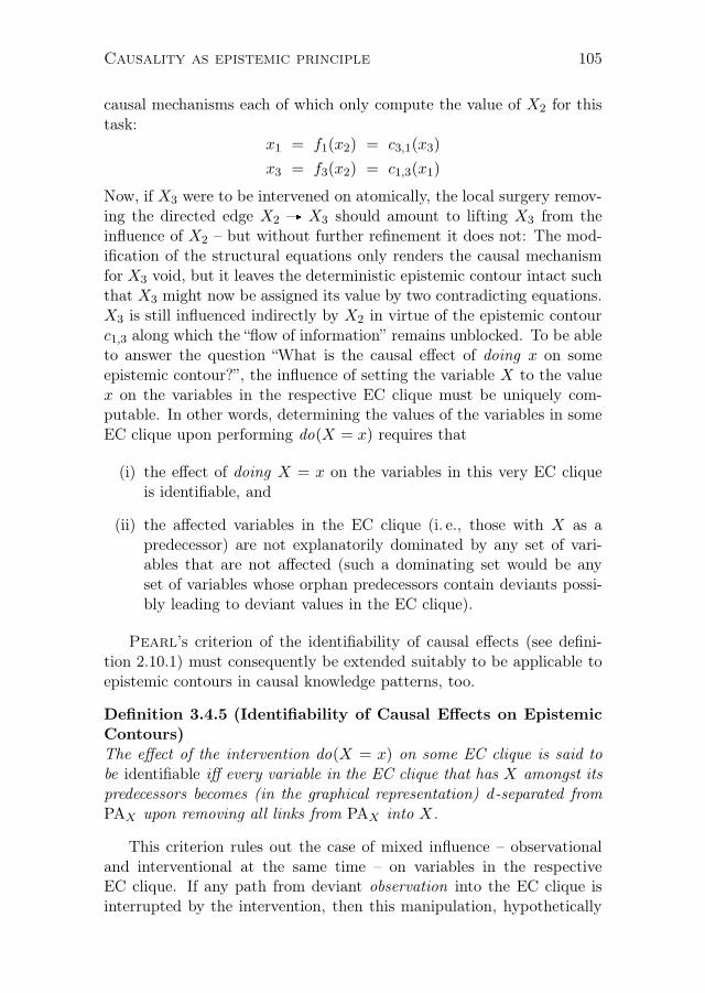
Causality as epistemic principle 105
causal mechanisms each of which only compute the value of X2 for thistask:
x1 = f1(x2) = c3,1(x3)
x3 = f3(x2) = c1,3(x1)
Now, if X3 were to be intervened on atomically, the local surgery remov-ing the directed edge X2 A X3 should amount to lifting X3 from theinfluence of X2 – but without further refinement it does not: The mod-ification of the structural equations only renders the causal mechanismfor X3 void, but it leaves the deterministic epistemic contour intact suchthat X3 might now be assigned its value by two contradicting equations.X3 is still influenced indirectly by X2 in virtue of the epistemic contourc1,3 along which the “flow of information” remains unblocked. To be ableto answer the question “What is the causal effect of doing x on someepistemic contour?”, the influence of setting the variable X to the valuex on the variables in the respective EC clique must be uniquely com-putable. In other words, determining the values of the variables in someEC clique upon performing do(X = x) requires that
(i) the effect of doing X = x on the variables in this very EC cliqueis identifiable, and
(ii) the affected variables in the EC clique (i. e., those with X as apredecessor) are not explanatorily dominated by any set of vari-ables that are not affected (such a dominating set would be anyset of variables whose orphan predecessors contain deviants possi-bly leading to deviant values in the EC clique).
Pearl’s criterion of the identifiability of causal effects (see defini-tion 2.10.1) must consequently be extended suitably to be applicable toepistemic contours in causal knowledge patterns, too.
Definition 3.4.5 (Identifiability of Causal Effects on EpistemicContours)The effect of the intervention do(X = x) on some EC clique is said tobe identifiable iff every variable in the EC clique that has X amongst itspredecessors becomes (in the graphical representation) d-separated fromPAX upon removing all links from PAX into X.
This criterion rules out the case of mixed influence – observationaland interventional at the same time – on variables in the respectiveEC clique. If any path from deviant observation into the EC clique isinterrupted by the intervention, then this manipulation, hypothetically

106 Causality as epistemic principle
performed, may account for change in the EC clique. The values affectedby the intervention will now determine the values of all other variablesin this EC clique according to the following considerations, which shallbe split up into three cases, namely
A. direct interventions on EC clique variables,
B. single interventions above EC cliques, and
C. arbitrary compound interventions.
Case A. Direct interventions on EC clique variables. Any twovariables connected by an EC clique are strictly dependent, i. e., espe-cially in the case of an EC clique of simultaneously exogenous variablesit becomes obvious that the Markov assumption of mutual independenceis overridden (locally for these variables) but can in principle be regainedby postulating that setting one variable in this EC clique sets all variablesin this EC clique in accordance with the pertaining epistemic contours.29
In the case of inner epistemic contours, whatever the causal mechanismsmay be for each of the entry points into a specific EC clique, setting onevariable effectively means that the complete EC clique is lifted from theinfluence of the joint set of parents of all its variables. One variable couldnot be set to the desired value if some other causal mechanism were tointerfere, but if the structural surgery is carried out and the assignmentperformed, this must mean that no other influence overrides this inter-vention. Graphically, intervening on one variable within an EC cliquecuts all links into this very EC clique, which receives its compatible val-ues from the single do(·)-affected variable. Applying this principle tothe example above, intervening in the left graph of figure 3.4 by doingX3 = x3 will not only remove X2 A X3 but also cut out X2 A X1. Thevalue of X1 is consequently assigned by c3,1(x3) after setting X3 to x3.
Compound interventions, if directly performed on EC cliques, are ofcourse required to not oppose each other. The following example shallgive an illustration of how causal inference would be rendered impossibleif such opposing interventions were not ruled out. After that, the specialcase of ladder structures will be discussed in a second example below.
29Observing incompatible values in simultaneously exogenous EC clique variablescontradicts the CKP design in the first place and would naturally lead to dismissingthis structure.

Causality as epistemic principle 107
Example (Opposing interventions on EC clique variables)Consider the pair of epistemic contours ci,j/cj,i represented in the semi-DAG DK of the causal knowledge pattern K as the undirected edge c inthe structure Xi
cn Xj . This minimal EC clique is associated with thepair of mutual assignments
xi = cj,i(xj) and
xj = ci,j(xi).
Setting either variable to a constant value by external intervention si-multaneously determines the value of the second variable in accordancewith the system of equations above. Intervening on both variables at thesame time by joint manipulation causes trouble (in general) if the inter-ventions are performed independently, since Xi and Xj might be assignedvalues that are not compatible with the epistemic contour ci,j anymore(and cj,i, respectively), as in the following situation where the two di-chotomous variables Xi (taking distinct values xi or x′i) and Xj (takingdistinct values xj or x′j) are set simultaneously.
(i) ci,j = 〈xi, xj〉, 〈x′
i, x′
j〉
(ii) cj,i = c−1i,j
(iii) Simultaneous manipulations (compound intervention):do(Xi = xi) and do(Xj = x′j)
(iv) with do(Xi = xi): Xj assumes ci,j(xi) = xj
(v) with do(Xj = x′j): Xi assumes cj,i(x
′
j) = x′i
Lines (iv) and (v) make the contradiction obvious: Setting the variablesin opposition to each other (‘opposed’ relative to ci,j/cj,i) makes the epis-temic system collapse and renders further consistent inference impossible.If hypothetical compound interventions are to be performed, at all, theyhave to be performed in mutual dependence, i. e., by (systematically orpragmatically) suitable restrictions embedded in the intuitions on whichthe epistemic contours are formulated in the first place.30
Example (Intervening in ladder structures)Consider the left diagram of figure 3.5, which exhibits a ladder struc-ture, possibly connecting two frameworks of description with epistemic
30This is quite in analogy with the systematical and mathematical constraint inPearl’s causal models that no variable can be intervened on by multiple interventionssetting opposing values simultaneously.

108 Causality as epistemic principle
contours bridging corresponding atomic events in both systems (frame-work A and B) along the development over time – the causal chainsX1 A X3 A X5 and X2 A X4 A X6 are multiply connected in thisgraph. At each stage of the system’s development knowledge may be ex-changed both ways.31 The causal histories on each side of the ladder are(on a higher level) as tightly connected as their components. Now, in-tervening on X2 by setting it to x2 should yield the same course of theworld as simply observing X2 = x2. X2 is an exogenous variable, after all(which also means that X1 and X2 are simultaneously exogenous). Thevalue of X1 must only be computed by drawing on c2,1, in other words,doing x2 also determines x1 and lifts both variables from the influenceof any potential latent background variable. If X4 is to be intervened on,however, merely pruning the link X2 A X4 will not suffice for lifting X4
from the influence of X2, since the path X2 n X1 A X3 n X4 remainsunblocked. Again, X3 and X4 are marked as variables that cannot be de-coupled and are only to be modified simultaneously. Consequently, doingx4 must also lift X3 from the influence of its parent variables (X1 in thiscase) and set X3 to c4,3(x4).
Case B. Single interventions above EC cliques. If the influenceof some variable to be intervened on on a specific EC clique is mediatedby causal mechanisms (i. e., by directed edges in the graph), then causalreasoning can only be carried out non-paradoxically in case that (i) theeffect (on the EC clique) to be made out is identifiable and (ii) the valuebrought about in the affected EC clique variables is not explanatorilydominated by any set of non-affected variables in the same EC clique.
Example (Testing effects on EC cliques with independent histories)Consider the middle diagram of figure 3.5 where the EC clique X5 n X6
is influenced along two separate causal histories that are purposely notlinked by further epistemic contours (e. g., between X1 and X2). Thesestrands might represent two alternative causal paths, e. g., two differentexperimental designs producing strictly correlated observations X5 andX6 (by actively deviating from the passive default situations in X1 orX2). X5 n X6 acts like a logical OR: Intervening on X3 will removethe directed edge X1 A X3 and virtually decouple the causal histories ofX5 and X6 (for X2 assuming its default value) by graphically removingthe entry link X4 A X6 (whose pertaining causal history – default incharacter – can be called irrelevant in the sense of def. 3.4.4).
31The epistemic contours depicted in the graph of figure 3.5 are labeled with thename of only one of the functions they represent – c1,2 also signifies c2,1 in accordancewith definition 3.3.2 above.

Causality as epistemic principle 109
X1
X3
X5
X2
X4
X6
c1,2
c3,4
c5,6
X1 X2
X3 X4
X5 X6
c5,6
X1
X2 X3
X4 X5
c4,5
Fig. 3.5: In ladder structures (illustrated in the left graph) information is ex-changed between both chains at each stage. The middle and the rightgraph show examples of differently structured causal histories leadingup to X4 and X5.
Example (Testing effects on EC cliques with converging histories)The right diagram of figure 3.5 shows an epistemic contour X4 n X5
whose variables’ causal histories converge in X1. Now, intervening onX1 does not pose any problem for the value assignment to X4 and X5,since the formulation of the systems of equations for each causal historywarrants consistent outcomes. Intervening on X3, however, cuts the linkX1 A X3 and might result in contradicting (incompatible) value assign-ments to X4 and X5, because X4 is still potentially influenced by X1 aswell. The effect of setting X3 to x3 is not identifiable in accordance withdefinition 3.4.5 above: Pruning X1 A X3 does not lift X4 from the in-fluence of PA3 (X3’s parents), and X3 is at the same time an element ofthe set of X4’s predecessors.32
Intervening on X2, however, will result in removing the edges X1 A X2
and X3 A X2 simultaneously such that the effect of do(X2 = x2) on theEC clique X4 n X5 is analyzed as identifiable. Now, if X1 exhibits itsdefault value, X5 will also, and the set X5 will consequently not ex-planatorily dominate the set X4 of variables affected by doing x2. Thecausal history of X5 will be rendered void by removing the edge X3 A X5
32This analysis is analogous to applying Pearl’s criterion for the identifiabilityof causal effects (see definition 2.10.1) together with the back-door criterion (seedefinition 2.10.2) in Bayes net causal models without undirected edges; the analogycan be seen directly when X4 and X5 are pulled together into a compound node.

110 Causality as epistemic principle
(thereby re-establishing the extended Markov restriction for world ω withX1 at its default value and attributing explanatory power to X4 with itspertaining history).
Case C. Arbitrary compound interventions. Performing multipleinterventions simultaneously can be done by securing the above condi-tions (i. e., identifiability and non-dominatedness) under the additionallyimposed restriction that – as in the case of intervening on EC cliques di-rectly – arbitrary interventions must not lead to opposing values withinthe same EC clique, i. e., the set of affected variables in some specificEC clique may only show compatible values upon intervening. Then, asbefore, all remaining causal histories (if they do not produce a set of ex-planatorily dominating variables) may be deactivated by removing theirentry links to the EC clique under consideration. Again, this ensuresconsistent causal inference and explicates graphically what decouplingexperimental designs means.
In conclusion, all the above cases show how consistent inference from typecausal structures becomes partly relativized to token causal findings inthat the default situations mark certain subsets of possible worlds (i. e.,courses of events) and thereby facilitate prediction, explanation, and –ultimately – compact formulation of target-oriented strategy even in thecase of independent alternative causal histories.
From epistemic contours onwards
When considering edges directed away from EC cliques, things standdifferently. The right diagram of figure 3.4 shows the situation whereinformation from the EC clique is jointly used for the computation ofX2’s value x2. In this case, X2 seems to be jointly causally influencedby both of its parents, and intervening on X2 correctly lifts it from theinfluence of its parents, but the formulation of the causal mechanismpertaining to X2 can be reduced in the following manner:
x2 = f2(x1, x3)
= f2(x1, c1,3(x1)) = f ′2(x1)
= f2(c3,1(x3), x3) = f ′′2 (x3)
This shows that one of the arrows pointing towards X2 is superfluous forthe propagation of knowledge, i. e., this piece of structural informationdoes not give us any additional computational information we did not

Causality as epistemic principle 111
have before. The value of X2 can be calculated from one of the nodeswithin the EC clique alone. Since all epistemic contours are just asstable and autonomous as the causal mechanisms in the causal knowledgepattern, one of the functions of the pair c1,3/c3,1 can thus be codedinto f2 directly, which basically makes f2 a function of x1 alone (of x3,respectively), as given above by f ′2 (by f ′′2 , respectively). One of the linksX1 A X2 or X3 A X2 can thus be called a pseudo-link just as a directednode connection that is removed in the process of refining the model –going from the fully connected graph to a slimmer version – aiming atspecifying the examined situation in the most informative way for thederivation of meaningful causal claims. In the case of slimming down thefully connected directed graph just as in the case of deleting superfluouspseudo-links, the principle of Occam’s razor and good implementationpractice tell us that introducing (or upholding) redundant information isto be avoided.33 I believe this idea also appertains to the features of theeconomical principle of knowledge organization called causality in thisaccount. As a structural rule, collider nodes in a semi-DAG linked tomore than one parent node of the same EC clique may in many cases bereduced away for reasons of economy (unless associations along differentpaths are precisely to be emphasized as in cases of decision making, seesection 4.1).
Mimicking hypothetical interventions and learning by ab-
duction
The above explications elaborate how contradictory conclusions fromknowledge represented in causal knowledge patterns can be avoided byadding one more ingredient – default assignments. If observation is over-ridden by external manipulation, though, testing for compatible valuesin epistemic contours helps the researcher rule out contradictory exper-iments (relative to a subset of possible worlds) or experimental designsaltogether (if two independent designs never yield consistent values oronly trivially in one marked possible world). The question, what manip-ulations go together well and what manipulations are to be avoided forwhich obtaining observations is answered by the above rules.
33Note that introducing epistemic contours is not understood as falling under thisverdict in the first place, since the variables connected by epistemic contours stillconvey intensional knowledge and additional connotations that might be exploited inthe further augmentation of the causal knowledge pattern under consideration. Thisdoes not hold for superfluous directed edges as in the example, since they can bereduced mathematically. Also see Pearl’s short remark on model preference andOccam’s razor in [Pearl 2009, sect. 2.3, pp. 45 ff.].

112 Causality as epistemic principle
Turning this very question around, one might consider epistemic contoursthat bridge technical or descriptive frameworks within one causal knowl-edge pattern such that, e. g., Xi
cn Xj represents this inter-frameworkbridge with Xi belonging to framework A and Xj belonging to frame-work B. When manipulating the direct causes of Xi within frameworkA, a typical answer we might look for now is what the corresponding in-tervention in framework B would be in order to bring about Xj . Causalknowledge patterns serve as oracles of abduction for this kind of coun-terfactual deliberations.
X1
X2 X3
X4 X5
c
do(X1 = x1)
x3 = c2,3(f2(x1)) = f3(x4, x5)
Fig. 3.6: Intervening on the variable X1 in the semi-DAG given here yieldsknowledge about possible interventions “across c” that would be nec-essary to bring about some realization of X3 directly through jointmanipulation of X4 and X5.
The illustration in figure 3.6 shows a semi-DAG with the epistemiccontour c possibly bridging two descriptive frameworks A and B withX1, X2 situated in framework A and X3, X4, X5 in framework B. In-tervening on X1 by doing X1 = x1 enables us to read off the graph thevalue of X3 computable by x3 = c2,3(x2) (where x2 is calculated throughx2 = f2(x1)). The given causal knowledge pattern marks X4 and X5 asdirect causes of X3, setting X3’s value according to the causal mecha-nism f3, such that x3 = f3(x4, x5) when the arrows pointing towardsX3 are not removed but kept intact. Having all this knowledge at handmakes the causal knowledge pattern an informant about hypotheticalinterventions in framework B that entail the same assignment to X3 asthe one just brought about indirectly by hypothetical intervention withinframework A. The set of possible, simultaneous compound interventionson X4 and X5 entailing X3’s realization c2,3(f2(x1)) is the set
−1f3 [c2,3(x2)]

Causality as epistemic principle 113
which is the set of inverse images of c2,3(x2) under f3, defined by
−1fj [ci,j(vi)] = paj | fj(paj) = ci,j(vi)
with fj being the causal mechanism for Vj and paj representing the(vector of) values of all parents (i. e., direct causes) of Vj .
34 Of course,iterated application of this abductive step will yield information aboutcausal histories of any length.35
3.5 Reviewing the framework
Someone objecting to the implementation of epistemic contours in anextension of the manipulationist Bayes nets framework might argue thatthe nodes of one EC clique represent events that are not distinct – quiteon the contrary, they are even strictly correlated – and should as suchnot be included in a well-designed causal model. The critic might add,there is nothing more to causal dependence than given in Bayesian nets,and epistemic contours or the intuition behind those should merely beguidelines in the modeling process, which ultimately yields well-knownstandard Bayes net causal models with all nodes denoting extension-ally disjoint regions in spacetime.36 This all might be crucial consid-erations in the business of equipping robots or inference machines withbasic constraints on what to read off the noise acquired through theirsensors – on whatever level of abstraction these might operate. In thecase of tracing the mechanics of human causal reasoning (expressed ineveryday language or specialized jargon), things lie differently. Pearl
himself emphasizes the recourse to basal causal assumptions when theepidemiologist builds a causal model or when we discuss politics in pri-vate. If the intuitions behind epistemic contours serve as guidelines inthis modeling process, they might as well be embedded in a suitablymodified framework that allows for making explicit how we arrive at theblueprints of interrelated events structured by causal knowledge. Largeportions of what we know about the relations of the events surroundingus is built upon non-causal data, i. e., as in the current proposal, deter-ministic non-directional knowledge. Epistemic contours, as introduced
34This notation is adapted from [Link 2009, p. 433] where Link defines the set
“Urbildmenge von B unter f ” as−1
f [B] := x | f(x) ∈ B.35See also sect. 2.11 for a presentation of Pearl’s adaptation of the concept of
abduction to the analysis of actual causes in epistemically related twin networks.36For a discussion of discerning events and times in the business of causal modeling
see [Hitchcock (forthcoming)].

114 Causality as epistemic principle
above, are included in shared bodies of information either (i) tentativelyuntil theories are unified or concepts matched and labeled with the samename tag (thereby reducing the contents of the model to extensionallydisjoint denotata) or (ii) purposely to mark intensions, aspects, perspec-tives, jargon, or frameworks or (iii) even because spatio-temporal localityor contiguity seems to be violated in the setting under consideration andthe purely mechanistic framework fails to yield some insightful rendition.The embedding of non-causal knowledge for causal inference and for com-municating (indirect) causal relations is facilitated by construing causalknowledge patterns in the unified formal system proposed above.37
The approach given here accounts for causal relations as epistemic re-lations by which knowledge is organized efficiently. It can be understoodas a uniform account that does not treat causal claims pluralisticallywithin their respective domains but on the contrary facilitates the unifi-cation of heterogeneous levels or disciplines in the same formal structure.Causal inference remains frame-relative with the shape of those framesbeing due to our cognitive faculty of carving out subsystems from whatwe perceive around us.38 This does not put off events to the realm ofpure imagination (or mental representation) but allows us to retain asolid event realism such that causal relations epistemically hold betweenrepresentations of real (i. e., physically ontological) events. FollowingPearl, analysis builds upon type knowledge and goes from there to to-ken claims. It does so non-reductively in one sense – with causation beingdefined in terms of basal causal assumptions – and reductively in another– by deriving higher-level causal claims from lower-level ones. Causal-ity becomes an epistemic principle of organizing knowledge efficiently byordering it deterministically – always with the possibility of also eval-uating probabilistic causal claims as propagation of belief blurred byunmeasured influences. Relying on the Bayes net framework, the CKPtoolbox can readily be applied to the same settings as causal models.It will, however, be able to also treat examples that incorporate eventswhich are entangled in epistemic manner or only turn out to be so invirtue of the extended capabilities of causal knowledge patterns.
37Point (i) above contains that in the CKP framework knowledge used for makingcausal claims can be explicated formally as a basis for experts to start disentangling(or unifying) variables – maybe of different levels of explanation – to tell us howthings work physically ontologically if this is the aim of research and if the situationunder consideration permits such an analysis, at all.
38Questions of model evocation and model revision must be put aside here to furtherexaminations in induction, abstraction, and belief revision.

Chapter 4
Modeling with causalknowledge patterns
What our eyes behold maywell be the text of life butone’s meditations on the textand the disclosures of thesemeditations are no less a partof the structure of reality
Wallace Stevens, ThreeAcademic Pieces – no. 1
4.1 Causal decision theory, or:
Of prisoners and predictors
Decision theory in general examines the rational principles guiding thedecisions that aim at the attainment of one’s goals. Causal decision the-ory does so by taking one’s act’s consequences into account – rationallychoosing an option must be based on the available knowledge about thecausal relations in the respective situation, so the argument goes. Oneof the principles taken to be a measure for rationality is the option ofmaximizing the utility of the outcome, i. e., by making the outcome equalor better than if one had chosen a different alternative for action. Prob-abilities and utilities are used to compute an act’s expected utility suchthat – as emphasized in causal decision theory – dependence betweenacts and outcomes are understood as of causal (asymmetrical) character

116 Modeling with causal knowledge patterns
– contrary to a merely evidential theory of decision making. A secondprinciple of rationality dictates choosing the course of action that is bet-ter, regardless of what the world is like. This principle of dominanceseems to be in conflict with the above-mentioned principle of expected-utility maximization in the curious case of Newcomb’s paradox.
Newcomb, Nozick, and a problem
Referring back to the physicist William Newcomb, who first formulatedthis dilemma for decision theory, Robert Nozick elaborates on – as hecalls it – Newcomb’s problem, in which two principles of rational choiceseemingly conflict each other, at least in the numerous renditions in thevast literature on this topic.1
In Newcomb’s problem some human-like agent plays a game againstsome daemon predictor that influences the course of the game upon pre-dicting his opponent’s move. The agent may choose to take either oneor two boxes in front of him – either box 1 only or box 1 and 2 together.In doing so he has no knowledge about the contents of the opaque box 1,but he can see one thousand dollars lying in box 2. If the daemon pre-dicts that the agent will take only one box (i. e., box 1), he will putone million dollars in the opaque box 1. The daemon will put nothingin box 1, though, if he foresees the agent taking both boxes. The pre-diction is reliable, or as Nozick introduces the predictor, “[o]ne mighttell a longer story, but all this leads you to believe that almost certainlythis being’s prediction about [the agent’s] choice in the situation to bediscussed will be correct.”2 Moreover, the agent has perfect knowledgeof all these features of the decision game he finds himself in.3
The possible outcomes of the game are presented in table 4.1 where therows stand for the agent’s options, the columns partition the world inpossible states, and each cell contains the sum our agent receives uponchoosing an action in some state of the world.
1Cf. [Nozick 1969] for the original presentation of the paradox and [Weirich 2008]for an overview on various suggestions of how to solve the Newcomb case.
2Cf. [Nozick 1969, p. 114].3Note that for reasons of simplicity this presentation of the Newcomb game situa-
tion slightly (but inessentially) differs from the way Nozick originally presents it in[Nozick 1969].
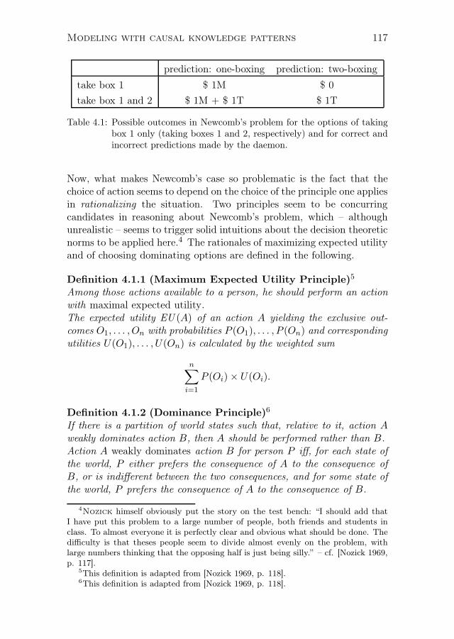
Modeling with causal knowledge patterns 117
prediction: one-boxing prediction: two-boxing
take box 1 $ 1M $ 0
take box 1 and 2 $ 1M + $ 1T $ 1T
Table 4.1: Possible outcomes in Newcomb’s problem for the options of takingbox 1 only (taking boxes 1 and 2, respectively) and for correct andincorrect predictions made by the daemon.
Now, what makes Newcomb’s case so problematic is the fact that thechoice of action seems to depend on the choice of the principle one appliesin rationalizing the situation. Two principles seem to be concurringcandidates in reasoning about Newcomb’s problem, which – althoughunrealistic – seems to trigger solid intuitions about the decision theoreticnorms to be applied here.4 The rationales of maximizing expected utilityand of choosing dominating options are defined in the following.
Definition 4.1.1 (Maximum Expected Utility Principle)5
Among those actions available to a person, he should perform an actionwith maximal expected utility.The expected utility EU (A) of an action A yielding the exclusive out-comes O1, . . . , On with probabilities P (O1), . . . , P (On) and correspondingutilities U(O1), . . . , U(On) is calculated by the weighted sum
n∑
i=1
P (Oi)× U(Oi).
Definition 4.1.2 (Dominance Principle)6
If there is a partition of world states such that, relative to it, action A
weakly dominates action B, then A should be performed rather than B.Action A weakly dominates action B for person P iff, for each state ofthe world, P either prefers the consequence of A to the consequence ofB, or is indifferent between the two consequences, and for some state ofthe world, P prefers the consequence of A to the consequence of B.
4Nozick himself obviously put the story on the test bench: “I should add that
I have put this problem to a large number of people, both friends and students inclass. To almost everyone it is perfectly clear and obvious what should be done. Thedifficulty is that theses people seem to divide almost evenly on the problem, withlarge numbers thinking that the opposing half is just being silly.” – cf. [Nozick 1969,p. 117].
5This definition is adapted from [Nozick 1969, p. 118].6This definition is adapted from [Nozick 1969, p. 118].

118 Modeling with causal knowledge patterns
Let us take ‘reliable’ (as ascribed to the daemon’s faculty of foreseeingfuture events) at face value and compute the expected utility for theoutcome of each specific course of the game – the unit of the expectedutility being dollars in our case. Assuming a reliable daemon basicallyamounts to saying that the act of taking one or both boxes and theprediction of this very act are highly correlated such that acts in statesof the world with incorrect predictions receive a probability of 0, whereasmatching acts and predictions receive the probability of 1. Table 4.2shows the expected utilities for all four thinkable courses of the gamewith one option clearly to be preferred over all others: The agent shouldtake only the opaque box and can then be certain of winning $ 1M, whichclearly supercedes the alternatives as maximum expected utility.
prediction: one-boxing prediction: two-boxing
take box 1 $ 1M $ 0
take box 1 and 2 $ 0 $ 1T
Table 4.2: Computing expected utilities in the case of a perfectly reliable pre-diction yields the utility of $ 0 for all cells representing incorrectpredictions. Maximizing this expected utility amounts to choosingonly box 1.
Pondering a different approach to maximizing the outcome of thegame, Nozick tweaks the story a little: The predictor did make hisprediction a week ago, and it is now the agent’s turn to make up hismind and take either only the opaque box 1 or on top of that also thetransparent second box 2, which contains one thousand dollars openlyvisible to the agent. The money is already there and will not be taken outof the boxes anymore after the agent has made a decision. So, regardlessof the daemon’s prediction, adopting the principle of dominance forcesthe agent to take both boxes – he will always end up with one thousanddollars more than if he had only taken one box. Taking both boxes evenstrictly dominates the act of taking only one box as can be read off table4.1 by comparing an entry in the second line to the entry in the first linewithin the same partition of the world’s states.
Obviously, the principle of maximizing expected utilities and theprinciple of dominance yield opposing recommendations to the delib-erating agent. While standard evidential decision theory seems to leantowards one-boxing (taking an agent’s act as a sign of what the predictionmust have been), causal decision theorists clearly position themselves on

Modeling with causal knowledge patterns 119
the side of two-boxing (rejecting backward causation and understandingthe agent’s deliberate decision as cutting any connection between actand prediction). When Judea Pearl within his interventionist accountof causal reasoning discusses model-internal observed acts and model-altering actions from outside, he also comes to reflect upon the concep-tual difficulties hidden in Newcomb’s problem:
The confusion between actions and acts has led to Newcomb’s para-dox (Nozick 1969) and other oddities in the so-called evidential de-cision theory, which encourages decision makers to take into con-sideration the evidence that an action would provide, if enacted.This bizarre theory seems to have loomed from Jeffrey’s influentialbook The Logic of Decision (Jeffrey 1965), in which actions aretreated as ordinary events (rather than interventions) and, accord-ingly, the effects of actions are obtained through conditionalizationrather than through a mechanism-modifying operation like do(x).7
When Pearl goes on by comparing the maxims of evidential and causaldecision theory, he baldly comments in a footnote:
I purposely avoid the common title “causal decision theory” in orderto suppress even the slightest hint that any alternative, noncausaltheory can be used to guide decisions.8
To reconcile the dominance principle with the expected-utility princi-ple – and hence to dissolve the paradox in Newcomb’s case – has beenthe aim of quite a few proposals, which nevertheless arrive at differentconclusions.
Conditionals and causal graphs
In A Theory of Conditionals (1968) Robert Stalnaker suggests a for-mal framework for analyzing the truth of counterfactual statements (sub-junctive conditionals) quite similar to Lewis’ proposal sketched above –‘If A, then B’ is assigned a truth value in accordance with the followinginformal condition:
Consider a possible world in which A is true, and which otherwisediffers minimally from the actual world. ‘If A, then B’ is true(false) just in case B is true (false) in that possible world.9
7Cf. [Pearl 2009, p. 108].8Cf. [Pearl 2009, p. 108, footnote 1].9Cf. [Stalnaker 1968, p. 169].

120 Modeling with causal knowledge patterns
The subjunctive connective ‘>’ is subsequently equipped with the moreformal semantical rules
A > B is true in α if B is true in f(A,α) andA > B is false in α if B is false in f(A,α),
where α is a possible world, the base world, and β = f(A,α) representsthe selected world minimally differing from the actual world in which B
is evaluated (with f being the selection function operating on a suitablesimilarity ordering of possible worlds).
Now, in his Letter to David Lewis (1972) Stalnaker suggests away of calculating expected utilities in the Newcomb problem that usesprobabilities of subjunctive conditionals instead of standard conditionalprobabilities.10 The expected utility of some action A would then becomputed the following way:
EU (A) =
n∑
i=1
P (A > Si)× U(A&Si),
where n signifies the amount of states S the world is partitioned into,i. e., n = 2 for the two possible predictions ‘one-boxing’ (i = 1) and‘two-boxing’ (i = 2). As Stalnaker argues, the agent’s action does notcause the daemon’s prediction made in the past, and hence the probabil-ity of the conditional equals the probability of the prediction alone. Butthis sets all probability terms in the sum formula above to equal values– the utilities can just be read off the corresponding cells in table 4.1.Two-boxing’s expected utility will always be greater then one-boxing’sexpected utility. Following Robert Stalnaker’s suggestion of inter-preting the involved probabilities causally, the maximization of expectedutility and the dominance principle recommend taking the same action:two-boxing.
Applying causal decision theory to Newcomb’s problem has been crit-icized by many authors – mainly because it yields the counter-intuitiverecommendation of taking both boxes, which nevertheless remains as theonly rationally explained choice given the circumstances of Newcomb’sproblem with decisions screening off acts from any previous events, ascausal decision theorists claim. In his seminal book The Foundations ofCausal Decision Theory James Joyce clearly states his position on theissue:
10Cf. for this and the following [Weirich 2008, sect. 2.2].

Modeling with causal knowledge patterns 121
When the evidential and the causal import of actions diverge [. . . ],the evidential theory tells decision makers to put the pursuit ofgood news ahead of the pursuit of good results. Many philosophers,I among them, see this as a mistake. Rational agents choose actson the basis of their causal efficacy, not their auspiciousness; theyact to bring about good results even when doing so might betokenbad news.11
While, e. g., David Lewis and Brian Skyrms in their accounts markattainable situations by building causal information into states of theworld and thereby reconcile the above otherwise diverging principles ofrational choice in the recommendation of two-boxing, Ellery Eells in hisconsiderations arrives at the same conclusion without drawing on the no-tion of causality. He claims that mere reflection on the available evidencewill force the agent to rationally go for both boxes – even more directwithout the recourse to any causal theory. Quite in this line of reasoningRichard Jeffrey also eliminates any hint of a causal nexus betweenthe events in Newcomb’s problem for the sake of a less metaphysicallycharged analysis. Pondering the Newcomb case Jeffrey seems to oscil-late between one-boxing and two-boxing to later arrive at the conclusionthat the story, presented this way, is a somehow illegitimate decisionproblem with the freely deliberating agent not capable of freeing hisdecision from being correlated with the predictor’s prediction.12 TerryHorgan and Paul Horwich take the Newcomb plot at face value andpromote one-boxing, simply because one-boxers ultimately take moremoney home, as the story is told. Paul Weirich diagnoses dryly: “Themain rationale for one-boxing is that one-boxers fare better than do two-boxers. Causal decision theorists respond that Newcomb’s problem is anunusual case that rewards irrationality. One-boxing is irrational even ifone-boxers prosper.”13
Having developed his ranking theory as a tool for epistemology andcausal analysis,14 Wolfgang Spohn positions himself on the side of causal(vs. evidential) decision theory and had been a strong advocate of two-boxing for a long time before he started “Reversing 30 Years of Discus-sion” by presenting an elaborate argumentation “Why Causal DecisionTheorists Should One-Box.”15
11Cf. [Joyce 1999, p. 146].12Cf. e. g. [Joyce 2007].13Cf. [Weirich 2008, sect. 2.5].14Cf. Spohn: Ranking Theory (forthcoming).15The quotations here refer to the title of [Spohn (forthcoming)].

122 Modeling with causal knowledge patterns
P
M
B
P
M
B
P
M
B
B∗
(i) (ii) (iii)
Fig. 4.1: Wolfgang Spohn discusses the usual manipulated (mutilated) causalgraph (i) employed by causal decision theorists for the analysis of theNewcomb problem, the decision graph (ii) for the same situation, andthe reflexive decision graph (iii) augmented by the decision node B∗.
Figure 4.1 illustrates the golden thread in Spohn’s chain of reason-ing. Time evolves from top to bottom in all three diagrams. The leftdiagram (i) shows the standard rendition used by causal decision the-orists for the analysis of the Newcomb problem – this mutilated causalgraph contains the node P representing the daemon’s prediction as thefirst event in time before action node B (representing the agent takingone or two boxes) and the bottom node M (for monetary outcome).The diagram is mutilated quite in agreement with Pearl’s intervention-ist framework: The hypothetical local surgery, i. e., the intervention onB, prunes any arrows possibly pointing towards B, thereby freeing thisnode from the influence of any other node in the model and making thecorresponding variable an exogenous one. The course of action can nowbe chosen on the basis of this decision graph, in which the wiggled vari-able is graphically represented by the square node. This rendition followsthe two decision theoretic principles highlighted by Spohn in this con-text: “acts are exogenous” and – derived from the first – “no probabilitiesfor acts.” Of course, Spohn’s acts have to be interpreted as Pearl’sactions (i. e., acts in mutilated models). Whatever the connection be-tween nodes P and B might have been in some graphical rendition of theoriginal causal relations understood as representing the Newcomb plot(e. g., with P as a direct cause of B), graph (i) in figure 4.1 representsthe variables’ dependencies once the agent deliberately takes action. Pand B are d-separated (by the collider in P A M B B), which makesthe choice of taking both boxes rational – whatever has been put into theboxes (based upon the prediction early in the game) will not become lessby choosing either one or, alternatively, two boxes (later in the game).

Modeling with causal knowledge patterns 123
Spohn declares himself dissatisfied with this analysis and brings upthe mind-bugging questions about the reliability of the daemon, again:
What about the remarkable success of the predictor that suggeststhat given you one-box it is very likely that she will have predictedthat you will one-box, and likewise for two-boxing? How do theyenter the picture? They don’t. [Causal decision theorists] do notdeny them, but they take great pains to explain that they are not theones to be used in practical deliberation calculating expected utili-ties; and they diverge in how exactly to conceive of the subjectiveprobabilities to be used instead.16
If the causal graph contained one more arrow from B to P , making theagent’s action a direct cause of the daemon’s prediction (as illustrated infigure 4.1, diagram (ii)), we would inevitably introduce backward causa-tion into the analysis. Spohn wants to avoid this but interprets graph (ii)as the decision-guiding pattern which the agent uses to choose betweenalternative actions – in Spohn’s terms: the ordinary decision graph forNewcomb’s problem. How are the causal relations laid out, however?If neither the prediction causes the agent’s act nor this act can causethe daemon’s prediction, we have to infer the existence of an earlierthird event as a common cause of both P and B – quite in accordancewith Reichenbach’s Common Cause Principle. Spohn’s straightfor-ward suggestion is to understand the decision situation the agent findshimself in as the common cause in question. This decision situationB∗ (as introduced into graph (iii) in figure 4.1) might consist of all theagent’s beliefs, prior knowledge, or rational principles the agent may noteven be aware of (the daemon is, however) but which he will without failemploy in deciding about his strategy B when standing before the twoboxes. In particular, B∗ also contains the full ordinary decision-guidingpattern (ii), which makes graph (iii) a reflexive decision graph containinga reduced version of itself.17 Making this move, Spohn openly rejects the“acts are exogenous” principle. An agent’s strategic deliberation aboutalternative courses of action does not decouple the act from past or fu-ture events – he might, quite on the contrary, make his deliberationsdepend on (i. e., graphically speaking, link them to) predecessor nodes inthe diagram. He might, on top of that, also be aware of the probabilitiesof different actions he may choose from, knowing what he usually doesor intentionally avoids in normal cases etc. There might be probabilities
16Cf. [Spohn (forthcoming), p. 4].17
Spohn gives clear rules for the step-wise reduction of a reflexive decision graphto its ordinary counterpart possibly containing backward links – cf. [Spohn (forth-coming), sect. 3].

124 Modeling with causal knowledge patterns
for the agent’s act, after all. Querying Spohn’s reflexive decision graphon the ground of all these considerations ultimately yields the recom-mendation of one-boxing – after reflecting on the current situation (inB∗), the rational agent must come to the unequivocal conclusion thatdeciding to one-box and acting accordingly simply maximizes the utilityof his act B.
Let us compare Spohn’s analysis with Pearl’s causal maxims, oncemore. The ordinary decision graph (as displayed in figure 4.1.ii) fullycomplies with what Pearl would devise for strategic reasoning, i. e.,a graph that simulates possible outcomes of hypothetical interventions.Setting B tells us the value of M . B is an exogenous variable such thatthe “acts are exogenous” principle is adhered to – act and action amountto the same consequence in this case. The evidential and the causalapproach perfectly concord in this diagram, were it not for the directedbackward edge B A P . This is the reason for Pearl to think directlyin terms of the mutilated graph (given in figure 4.1.i) and for Spohn tocall diagram 4.1.ii not causal but reduced, ordinary decision graph. Inthe further step of construing the reflexive decision graph 4.1.iii, Spohn
must reject the “acts are exogenous” principle and convincingly arguesfor his case: The hypothetical intervention on the variable B must notbe performed within the reflexive decision graph. This graph makesexplicit what it means for the agent to be rational, i. e., he acts on hisknowledge, principles, and rational considerations given in B∗. Pruningthe link B∗ A B would make the agent plainly irrational and ignorant ofhis own situation, since the deliberation process is pushed into the model.
Technical answers to questions about how to properly reduce reflex-ive decision graphs to their ordinary, structural counterparts can all befound in Spohn’s explications. Conceptual questions remain, however.18
Firstly, the introduction of a common cause for B and P essentially addsto the Newcomb’s story the idea of being (perhaps physically determi-nately) pre-disposed. In a way, this metaphysically overloads the alreadyartificially construed plot with another element just by drawing on Rei-
chenbach’s principle of the common cause. Moreover, it forces Spohn
to set apart the agent’s inclinations to take certain actions from the actsthemselves. Decision making in the game is consequently re-interpretedas only discovering one’s previously fixed inclinations (where discovery is
18I am thankful to Wilken Steiner for valuable discussions of Newcomb’s problemand Spohn’s treatment of it.

Modeling with causal knowledge patterns 125
not something brought about actively, e. g., such that it would manifestitself in hypothetical test interventions, but simply a feature of persistentrationality becoming evident). This rendition seems very far from themuch more intuitive interventionist framework, which merely requiresthe agent to bear a confined mini laboratory in his head and turn theknobs therein – knowledge about the mechanisms will yield unique vir-tual outcomes and guide decision making. Nevertheless, Spohn’s com-plex reflexive decision graph does rest in its core on the very simpleordinary reduced decision graph (figure 4.1.ii) to which the whole bur-den of explanation is shifted, which shall be looked at more closely in thefollowing. What can be the content of this reduced graph, after all? Ifthe link B A P is dismissed as causal relation, of what nature can it be?If it, on the other hand, does stand for some hidden causal connectionand is dismissed as backward causation, it must represent a causal linkthrough some obscure common cause. If this common parent node ofboth P and B is the decision situation again – just as in the reflexivegraph on the meta level – analysis enters an infinite regress at this point.Only the interventionist approach could prevent this from happening bypruning B A P , but then this would already apply on the upper levelin the reflexive decision graph and conflict with Spohn’s final conclu-sion. If the supposed common cause in figure 4.1.ii is interpreted assome irreducible obscure past event or state whose existence just has tobe acknowledged and whose link to B shall not be interrupted, then howwould it be possible to perform hypothetical test interventions on thisvery node to virtually maximize the outcome? If reflecting on this graphultimately comes down to just observing the propagation of values, then,one has to conclude, Spohn’s suggestion is constrained to stay withinevidential reasoning.
Foreseeing acts, foreseeing actions19
What the backward link B A P in graph 4.1.ii can possible mean shallin the following be made explicit within the CKP framework, therebyideally revealing more about the nature of the paradox and hopefullyilluminating some more features of how we reason with (non-)causalknowledge. The causal knowledge pattern in figure 4.2 traces the storyof Newcomb’s problem by only referring to the events that actually arein the narration. The problem is not treated by tweaking the story butby choosing a framework fit to accommodate all relevant concepts.
19I have greatly benefitted from discussing Newcomb’s problem and the concept ofrationality with Olivier Roy for whose comments on this section I am very thankful.

126 Modeling with causal knowledge patterns
D
B
P1
P2
M
c
Fig. 4.2: Newcomb’s problem with the act of taking one or two boxes (B) de-terministically connected to the daemon’s reliable prediction (P1) byan epistemic contour (c) in this causal knowledge pattern.
Our human-like agent deliberates about the situation he finds himselfin and decides what to do (D), namely if he takes one box or both boxes(B). The daemon predicts what the agent will do (P1) and preparesthe boxes accordingly (P2). The monetary outcome (M) should finallyreward the rational agent. Time evolves from top to bottom in the di-agram.20 The vertical positioning of P2 is inessential for the analysis ofthe situation (P2 could as well come after B if the game is set up ina way that the agent only writes down his choice on a sheet of papersecretly in step B). The daemon’s prediction together with its reliabilityis interpreted in this causal knowledge pattern as an undirected 1-1 rela-tionship. Neither would we say that the agent’s act genuinely causes theprediction of this very act, nor does it sound right to say the predictioncauses the predicted event.21 But there is more in the pattern: B isnot directly linked to the daemon’s preparation of the boxes P2 – thisconnection is mediated by the prediction P1, which has direct causal in-fluence on P2 in turn. This is quite in agreement with Spohn’s analysisthat the causal structure of the Newcomb problem should exhibit somenode previous to both players’ acts in the game that at the same timetakes care of the bidirectional transfer of belief. P1 and P2 are separatedin the causal knowledge pattern for this very reason. On the other side,D (the human-like agent’s decision situation) and B (his concrete movein the game – either taking one or both boxes) are separated, as well, to
20Note that this diagram graphically reverses Spohn’s rendition where time evolvesfrom bottom to top.
21Moreover, as is argued here, drawing on Reichenbach’s Common Cause Princi-ple for an explication of ‘prediction’ is precisely a source of counter-intuitive inference.

Modeling with causal knowledge patterns 127
disentangle conceptually what it means for the agent to spontaneouslyand possibly unforeseenly change his mind. This is a much-discussedissue in the literature and does pose additional problems if the modelingallows for the agent changing his mind and the daemon’s prediction re-ferring to the ‘wrong’ decision. Not so in the suggested causal knowledgepattern, which links the prediction P1 to the agent’s final act B howeveroften he may have made up or changed his mind before actually takingonly one or, after all, both boxes. In other words, pondering courses ofaction must focus on B bearing the whole burden of explanation in theprocess of finding the best strategy for the maximization of the outcome.This is exactly as Nozick tells the story.
The modeling does not draw on the insertion of backward links thatwould signify backward causal flow. Nevertheless, information is trans-ferred back in time along the epistemic contour c, thereby formally grasp-ing the very meaning of ‘prediction.’ c will not get cut off by any localsurgery of the graph. By suitably applying hypothetical test interven-tions the following contents can be read off the causal knowledge pattern– quite in accordance with intuition:
• The agent’s decision (D) causes his act (B) – in general: any causalhistory of B naturally influences the agent’s act causally;
• the agent’s decision (D) is also interpreted as causing the daemon’speculiar prediction (P1) and thereby also as causing the daemon’sparticular move in the game (P2);
• intuition also conforms with the claim that the agent’s taking oneor two boxes (B) causes his antagonist’s preparation of the boxes– the predictor reacts to (B), after all;
• nevertheless, the agent’s act (B) does not cause its own peculiarprediction (P1) but determines it uniquely and – looking at the pat-tern from above – simultaneously though backwards through time.
Now, especially the last point reveals the core of the paradox andlocalizes the difficulties in reasoning about the causal relations involved.Any attempt of solving the artificial plot of Newcomb’s problem hingeson the question how to embed the concept of reliably predicting futureevents into the formal analysis (if such an analysis is not denied in thefirst place exactly because of the fictional character of the narration).The causal knowledge pattern above presents the prediction as the verything it is – an image of the agent’s act. Backward links are excludedfrom this rendition while querying the pattern does yield indirect causal
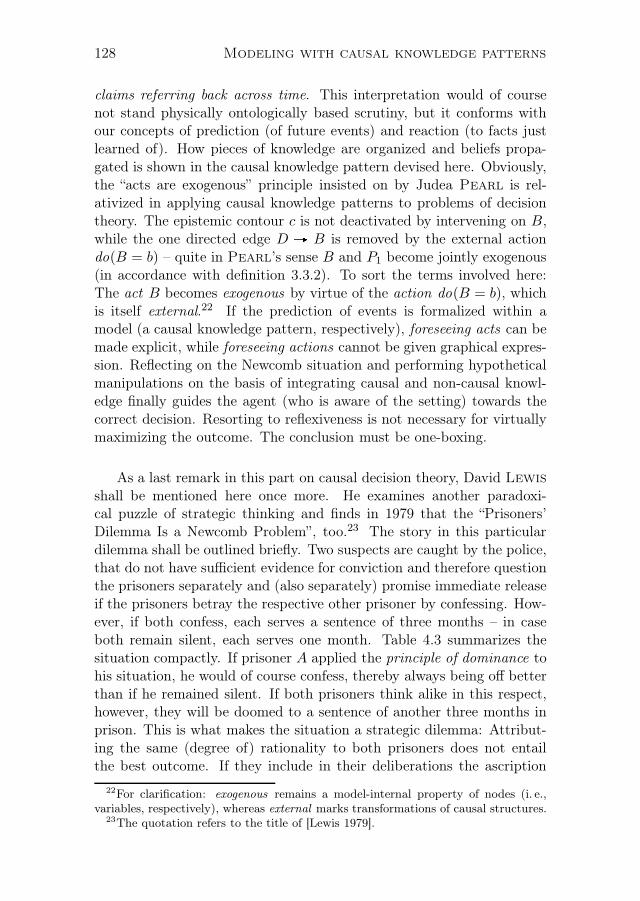
128 Modeling with causal knowledge patterns
claims referring back across time. This interpretation would of coursenot stand physically ontologically based scrutiny, but it conforms withour concepts of prediction (of future events) and reaction (to facts justlearned of). How pieces of knowledge are organized and beliefs propa-gated is shown in the causal knowledge pattern devised here. Obviously,the “acts are exogenous” principle insisted on by Judea Pearl is rel-ativized in applying causal knowledge patterns to problems of decisiontheory. The epistemic contour c is not deactivated by intervening on B,while the one directed edge D A B is removed by the external actiondo(B = b) – quite in Pearl’s sense B and P1 become jointly exogenous(in accordance with definition 3.3.2). To sort the terms involved here:The act B becomes exogenous by virtue of the action do(B = b), whichis itself external.22 If the prediction of events is formalized within amodel (a causal knowledge pattern, respectively), foreseeing acts can bemade explicit, while foreseeing actions cannot be given graphical expres-sion. Reflecting on the Newcomb situation and performing hypotheticalmanipulations on the basis of integrating causal and non-causal knowl-edge finally guides the agent (who is aware of the setting) towards thecorrect decision. Resorting to reflexiveness is not necessary for virtuallymaximizing the outcome. The conclusion must be one-boxing.
As a last remark in this part on causal decision theory, David Lewis
shall be mentioned here once more. He examines another paradoxi-cal puzzle of strategic thinking and finds in 1979 that the “Prisoners’Dilemma Is a Newcomb Problem”, too.23 The story in this particulardilemma shall be outlined briefly. Two suspects are caught by the police,that do not have sufficient evidence for conviction and therefore questionthe prisoners separately and (also separately) promise immediate releaseif the prisoners betray the respective other prisoner by confessing. How-ever, if both confess, each serves a sentence of three months – in caseboth remain silent, each serves one month. Table 4.3 summarizes thesituation compactly. If prisoner A applied the principle of dominance tohis situation, he would of course confess, thereby always being off betterthan if he remained silent. If both prisoners think alike in this respect,however, they will be doomed to a sentence of another three months inprison. This is what makes the situation a strategic dilemma: Attribut-ing the same (degree of) rationality to both prisoners does not entailthe best outcome. If they include in their deliberations the ascription
22For clarification: exogenous remains a model-internal property of nodes (i. e.,variables, respectively), whereas external marks transformations of causal structures.
23The quotation refers to the title of [Lewis 1979].
Modeling with causal knowledge patterns 129
of like-mindedness to their fellow inmate, both of them should remainsilent. If this ascription is reliable enough (or even deterministically cer-tain), e. g., because of some commitment to the same gang code, then theprediction in Newcomb’s problem and this theoretical simulation (the as-cription) in the prisoners’ dilemma essentially amount to the same thing– “[i]nessential trappings aside, Prisoners’ Dilemma is a version of New-comb’s Problem, quod erat demonstrandum.”24
B stays silent B confesses
A stays silent Each serves 1 m A serves 1 y, B goes free
A confesses A goes free, B serves 1 y Each serves 3 m
Table 4.3: Each of the prisoners could go free or serve a sentence of one month,three months, or a year – depending on their strategic decisions.
A common causal knowledge pattern might be used to capture all(non-)causal relations as in the above rendition of Newcomb’s problem– quite naturally and without introducing further metaphysical assump-tions about possible background variables. In fact, tilting the time axis infigure 4.2 by 90 degrees (such that time evolves from left to right) yieldsthe skeleton of the prisoners’ plot (of course, D and P2 are particularingredients of Newcomb’s problem and inessential for the current exam-ination). c represents the mutual ascription of like-mindedness of bothprisoners, who must decide to cooperate during their simultaneous (butseparate) questioning to achieve the joint best result. May the Newcombcase be some fictional construction, Lewis makes the case for analyzingthe prediction of future events and the ascription of like-mindedness toone’s antagonist in terms of the same underlying pattern:
Some have fended off the lessons of Newcomb’s Problem by saying:“Let us not have, or let us not rely on, any intuitions about whatis rational in goofball cases so unlike the decision problems of reallife.” But Prisoners’ Dilemmas are deplorably common in real life.They are the most down-to-earth versions of Newcomb’s Problemnow available.25
24Cf. [Lewis 1979, p. 239].25This final quotation borrows the concluding paragraph from [Lewis 1979, p. 240].
I agree with Lewis on the point that situations of strategic deliberations of thekind exemplified here are “the most down-to-earth versions of Newcomb’s Problem” –because there is nothing more to know than already said – in contrast to cases of so-called medical Newcomb problems where research might in most cases yield additionalinformation and knowledge about true common causes whose influence would indeedbe rendered void by free deliberation/active intervention.

130 Modeling with causal knowledge patterns
4.2 Meaningful isomorphisms
Augmenting standard Bayes nets by adding epistemic contours mightat first seem reducible again, as sketches of causal models (in Pearl’ssense) are refined and incorporated into scientific bodies of explanationor into strategic groundwork for policy making. The postulate of onlyadmitting extensionally distinct events in the analysis poses problems,though, as soon as intensional distinction becomes necessary or differentapproaches towards measuring the same phenomenon need to be em-phasized and unified in one frame. Epistemic contours pave the wayfor such enhanced modeling. As an additional structural component incausal knowledge patterns these 1-1 functions
• represent non-directional knowledge,
• are capable of bridging frameworks of description,
• deterministically transfer knowledge simultaneously,
• mark variables that cannot be decoupled (i. e., set separately),
• and are not deactivated by interventions, in particular.
Synonymy, strict semantical and conceptual dependencies, or logicaland mathematical relations present problems for the standard Bayes netapproach and are purposely excluded (by the expert modeler) from in-tegration into Pearl’s causal models. Representing such relationshipsas directed edges would subject them to possible local atomic surgeries,which would immediately yield paradoxical inferences. Including non-causal knowledge into the analysis, where information about isomorphicrelations is available, does essentially support causal inference, though,and can be computed consistently in the framework of causal knowledgepatterns – exemplary cases shall be considered in the following.
Synonyms
Two synonyms refer to the same phenomenon or to the same observationwhen they denote events, and are therefore modeled as just one nodein the graph of a causal model representing just one variable that canbe labeled differently but for which the specification of the method ofmeasurement fixes the extensional meaning. Epistemic contours can beused to accommodate more than one signifiant of one and the sameevent in the causal knowledge pattern, thereby bridging jargon, levelsof specialization, frameworks of distinct interests, differing aspects ofthe same research object, or intended systems of neighboring theories –

Modeling with causal knowledge patterns 131
Collisionof cloudparticles
Chargeseparationin cloud
Atmosphericelectrostaticdischarge
Ionizationof oxygenmolecules
Dinitrogenfixation
Formationof nitric
acid
Presenceof watermolecules
Lightning Thunder
c
Simple picture
Scientific pattern
Fig. 4.3: Frameworks of differing specialization are bridged by the epistemiccontour c representing an isomorphic relation between atmosphericelectrostatic discharge and lightning.
perhaps in the process of synthesizing.26 Figure 4.3 explicates this use ofepistemic contours: Two originally separate causal models are connectedthrough an epistemic contour c. The upper framework shows the fine-grained model of some bio-chemist who wants to trace the formationof nitric acid in the atmosphere. In the graph of his causal model thedirected edges represent causal mechanisms across the disciplines (quitein the sense of Jon Williamson, see also p. 90). Electro-magneticphenomena are linked to chemical processes in this scientific pattern,which does not pose any difficulty to the proponent of the epistemicaccount of causation. The lower causal model in figure 4.3 illustrates thesimple picture of how lightning and thunder might be arranged in somenaive (regularity) account (which possibly might not even be embeddableinto some more fine-grained scientific rendition). These two frameworksdo not talk about the same sets of phenomena, nor do they lie on the same
26Such epistemic bridges might lead to the discovery of more bridges between therespective frameworks. On the other hand, formalizing assumptions about the exis-tence of possible isomorphisms in this context can be of help for refuting these veryassumptions and for clarifying blurred differences between originally distinguishedtheoretical terms or cross-disciplinary “false friends.” Pragmatic examples can befound in pedagogical theories: One of the principles of neuro-didactics states thatlearning is more effective if existing prior knowledge is activated. How new informa-tion is connected with/augmented by/embedded in such prior knowledge or how it isto be re-ordered/aligned can be formalized in recourse to twin CKPs.

132 Modeling with causal knowledge patterns
level of specialization, and neither do their modelers “pursue commoninterests.” Nevertheless, as in this example, if the modelers agreed ona meta level to the fact that one of the phenomena their models areabout always co-occurs, the epistemic contour c shows how the differentframeworks can be aligned side by side for mutual information exchange.Thunder can subsequently be explained through the chain rooting inCollision of cloud particles.
Logical and mathematical dependencies
Any association between the description of two events that comes in theform of a parametric equation can in principle be represented by an epis-temic contour to facilitate causal reasoning across methods of measuringin cases where the introduction of a common cause seems far-fetched,artificial, or controversial. Scale translations (on the same level of mea-surement) can thus be given formal expression within causal knowledgepatterns, as well as unit conversions (e. g., of currencies) and geometrictransformations. Entities on both sides of such an epistemic contour ex-tensionally ‘measure one coin’ but intensionally emphasize ‘its differentsides’ – especially when these different characterizations invoke differingcausal claims. E. g., temperature (in ranges) and color (in name codes)of metal can be aligned side by side but might each be linked to differenteffects or even to different causes – according to the experimental setup.But knowledge about either tells the experimenters more about the ef-fects across the deterministic undirected edge in the causal knowledgepattern.27 Inversely proportional behavior is yet another candidate formodeling by epistemic contours (if the equation contains the total quan-tity as a parameter). When considering a certain country, the percentageof sealed soil determines what remains within the countries boundariesas a source of biomass and as a storage of nutrients, substances, water,etc. Neither causes the other – intervening on one determines the oppo-site. Both might be roots of differing causal chains, though, accordingto how knowledge is organized in some causal knowledge pattern, i. e.,within some epistemic subject.
27Transferring knowledge about the temperature over to knowledge about the colormight in addition require knowledge about the properties of the piece of metal un-der consideration. These properties are part of the parametric formulation of theisomorphism represented by the epistemic contour – they can be seen as a kind ofceteris paribus conditions if the experimental setup examines normal metal undernormal conditions. Parameters that can be modified through surgeries in the modelare excluded from the framework devised here but might motivate a possible furtherextension.

Modeling with causal knowledge patterns 133
Semantical and conceptual dependencies
Epistemic contours are also applicable to cases where interlevel causalclaims are to be rendered explicit – as one example of representing seman-tical dependencies by the introduction of an epistemic contour. WhenCarl Craver and William Bechtel talk about “levels of mechanisms,”they have in mind what Pearl would call zooming into (or zoomingout of) a given model to present the situation under consideration in amore fine-grained (or, respectively, in a more coarse-grained) variant.28
In their sense, a mechanism is a process as structured in a given causalmodel (in Pearl’s sense) and can as such be related to a more detailedor less detailed structure describing the same situation:
[L]evels of mechanisms are a species of compositional, or part-whole, relations. In contemporary debates about reduction and in-terlevel causation, it is common for authors to talk about ‘levelsof aggregation,’ ‘levels of organization,’ ‘levels of complexity,’ and‘mereological levels.’ Such descriptions apply to levels of mecha-nisms as well. Higher levels of mechanisms are aggregated (i. e.,built up from) or composed from parts that are organized into morecomplex spatial, temporal, and causal relations.29
In their discussion of both top-down and bottom-up causation theyclaim that causation across levels is described by what they call mecha-nistically mediated effects, which “are hybrids of constitutive and causalrelations in a mechanism, where the constitutive relations are interlevel,and the causal relations are exclusively intralevel.” They maintain fur-ther that the “[a]ppeal to top-down causation seems spooky or incoher-ent when it cannot be explicated in terms of mechanistically mediatedeffects.”30 In saying that, Craver and Bechtel refer back to DavidLewis who fixes intuitions about the distinctness of cause and effect inhis influential Causation as Influence:
C and E must be distinct events – and distinct not only in thesense of nonidentity but also in the sense of nonoverlap and non-implication. It won’t do to say that my speaking this sentencecauses my speaking this sentence or that my speaking the whole ofit causes my speaking the first half of it; or that my speaking causesmy speaking it loudly, or vice versa.31
28See also [Machamer et al. 2000] for a detailed overview of the concept of mech-anism in the sciences.
29Cf. [Craver & Bechtel 2007, p. 550].30Cf. [Craver & Bechtel 2007, p. 547].31This quotation is from the unabridged version of [Lewis 2000] as reprinted in
[Collins et al. 2004].

134 Modeling with causal knowledge patterns
The least disputed cases of genuine top-down or bottom-up causal rela-tions, where changing the system prima facie causally influences (at leastone of) its parts or vice versa, are figures of pars-pro-toto and totum-pro-parte reasoning. These cases can straightforwardly be translated into theframework of causal knowledge patterns by marking the level transitionwith an epistemic contour that represents the constitution (in Craver’sand Bechtel’s words) or the (mutual) constraint (as suggested by MaxKistler as a conceptual refinement in his comment32 on Craver andBechtel). Two examples shall be considered in the following.33
The general’s heart attack can be understood as a genuine pars-pro-toto figure, where the defect of the heart as part of the general’s bodydetermines the general’s state of being alive or dead. The biologicalintra-organism level and the level of the organism as a whole are linkedhere through 1-1 functional information exchange, not by any causalprocess. The general remains alive as long as (and only as long as) hisheart continues beating. This isomorphism is expressed in the pertainingcausal knowledge pattern as a simple epistemic contour, consequently.The story of Ignatius and his hotdogs on the other hand presents a cleartotum-pro-parte case where Ignatius maneuvers his hotdog cart to thecorner of the street to market his hotdogs there. Craver and Bechtel
ask: “What caused the hotdogs (and the molecules in the hotdogs, andthe atoms comprising the molecules, and so on) to arrive at the corner?Ignatius.” Although on different levels, Ignatius’ pushing the cart causesthe cart to move – and its parts and contents along with it. They aresimply “carried along for the ride.”34 An epistemic contour marks the 1-1non-causally interrelated positions of cart and hotdogs. Making Ignatiusmove the cart (“using a do(·)-operation on him”) will ultimately move hisgoods as well, which licenses the above claim about Ignatius as causeeon the lower level, too.
4.3 Epistemic contours and the Markov assump-
tion, revisited
Introducing epistemic contours as bridges of non-directional knowl-edge transfer into structures of causal reasoning was possible becausethese structures were understood as schemata of knowledge organization
32See [Kistler 2010] for Kistler’s explications.33For this and the following cf. [Craver & Bechtel 2007, pp. 557 ff.].34Cf. [Craver & Bechtel 2007, p. 558] for both quotations.

Modeling with causal knowledge patterns 135
shaped by the structuring power of the epistemically interpreted princi-ple of causality. The interventionist characterization of causation couldbe maintained by explicitly overriding the requirement that all variableshave to be modifiable separately – this is not the case for variables of anEC clique, where intervening on one distinguished variable strictly for-bids any opposing intervention on other variables in the same EC clique.Epistemic contours precisely postulate non-interruptibility of the deter-ministic functional connection they stand for. Their integration clasheswith the Markov assumption, because such epistemic contours might con-tradict the assignment of values through the causal mechanisms at work.By introducing the epistemic principle of explanatory dominance consis-tency is taken care of, again. Explicating causal with closely intertwinednon-causal knowledge in one unifying network makes the underlying as-sumptions concrete, transparent, and operative on the surface. Finally,the formal framework of causal knowledge patterns offers a means forconsistently deriving higher-level causal claims from basal data of dif-ferent types and might offer insight into dialectics of communicationand processes of learning. Adding structural ingredients and intensionalmarkers of default knowledge to standard Bayes net causal models alongwith the rules for implementation counters Pearl’s skepticism:
The Markovian assumption [. . . ] is a matter of convention, to dis-tinguish complete from incomplete models. By building the Marko-vian assumption into the definition of complete causal models [(def.2.7.1)] and then relaxing the assumption through latent structures[(see p. 66)], we declare our preparedness to miss the discoveryof non-Markovian causal models that cannot be described as latentstructures. I do not consider this loss to be very serious, becausesuch models – even if any exist in the macroscopic world – wouldhave limited utility as guides to decisions. For example, it is notclear how one would predict the effects of interventions from sucha model, save for explicitly listing the effect of every conceivableintervention in advance.35
What it means for an event A to cause some distinct event B isexplained above in terms of doxastic structures – how one predicts theeffects of interventions in causal knowledge patterns as compounds ofcausal and non-causal knowledge is described in interventionist vocabu-lary by extending the rules for the do(·)-operation. Drawing upon bodiesof epistemically organized relations precisely guides the epistemic sub-ject to decisions that might not be explainable as straightforwardly fromplain Bayes net structures.
35This quotes [Pearl 2009, p. 61] without footnotes.


Appendix A
Random variables(stochastic variables)
The Σ-random variable V over Ω is an 〈F ,X〉-measurable (total)function of the outcome of a statistical experiment, mapping possibleoutcomes to values (realizations, e. g., real numbers). The meaningof the random variable lies in the linkage between the outcome of anexperiment and its mathematical representation:1
V : Ω→ Σ
such that
V (ω) = σ or in short: V = σ or alsoV (ω) = v or in short: V = v (as commonly used),
with a probability space 〈Ω,F , P 〉 and an observation space 〈Σ,X〉, asexplained in the following.
The probability space is a triple 〈Ω,F , P 〉, where Ω is the samplespace Dom(V ) of a random process (sometimes also S for ‘sample space’or U for ‘universe’), and F ⊆ P(Ω) is the set of events (where eachevent is a set containing zero or more outcomes), the event algebra,a σ-algebra (σ-field or also borel field) over the set Ω, by definition anonempty collection of subsets of Ω (including Ω itself) that is closedunder complementation and countable unions of its members.
1Cf. for this and the following e. g. [Fahrmeir et al. 2000].

138 Random variables
E. g., for a given sample space Ω = a, b, c, d, F might be the subset ofP(Ω) specified as ∅, a, b, c, d, a, b, c, d. If we have F = P(Ω) inthe case of a finite sample space Ω, V is always measurable.
The probability function (the measure) P : F → [0, 1] defines a measureover F , satisfying the Kolmogorov axioms:
(K1) P (A ∈ F) ≥ 0,
(K2) P (Ω) = 1,
(K3) P (⋃
iAi) =∑
i P (Ai) for any countable sequence of pairwise dis-joint (i. e., mutually exclusive) events A1, A2, . . . (∈ F).
The measurable observation space (state space) 〈Σ,X〉 typicallycouples the real numbers R, the integers N, or any finite set of valueswith a suitable σ-algebra X over Σ with X ⊆ P(Σ):
for real-valued (continuous) random variables: V : Ω→ R;
for discrete random variables yielding values of countable sets, e. g.,of the set of natural numbers: V : Ω→ N;
and for dichotomous random variables: V : Ω→ 0, 1.
In this representation events are subsets of some sample space Ω, whichare also often written as propositional formulas containing random vari-ables, e. g., ω |u1 ≤ V (ω) ≤ u2, or shorthand: ω |u1 ≤ V ≤ u2.For the sample space Ω = ω0, ω1, . . . , ωn−1 with size n, the singletonsω0, ω1, . . . , ωn−1 are called ‘atomic events.’ Events A ⊆ Ω aredetermined by the random variable V , e. g., through formulations of thefollowing kind:
V = v := ω ∈ Ω |V (ω) = v,
V ≤ v := ω ∈ Ω |V (ω) ≤ v,
u1 ≤ V ≤ u2 := ω ∈ Ω |u1 ≤ V (ω) ≤ u2,
V ∈ I := ω ∈ Ω |V (ω) ∈ I,
where I is some specific interval.

Random variables 139
Example (Tossing a coin twice)A double coin toss may be modeled in the following probability space〈Ω,F , P 〉:
• Ω is the set of four possible outcomes:〈Heads,Heads〉, 〈Heads,Tails〉, 〈Tails,Heads〉, 〈Tails,Tails〉;
• F = P(Ω);
• for a fair coin, all possible atomic events are assigned equal proba-bility: P (〈N1,N2〉) = 1
4 for N1,N2 ∈ Heads,Tails.
The random variables X1, X2, and V are defined as follows:
1. X1 : Ω→ R such that 〈N1,N2〉 7→ 0, if N1 = Heads, 1 otherwise;
2. X2 : Ω→ R such that 〈N1,N2〉 7→ 0, if N2 = Heads, 1 otherwise;
3. V : Ω→ R such that V (ω) = X1(ω) +X2(ω) for any ω ∈ Ω;
and X is the borel algebra over the real numbers R.
Nota. For many applications it is not necessary – maybe not evenpossible – to find an underlying sample space (as it is in the examplesof tossing a coin or rolling a dice). Nevertheless, parameters of interest(e. g., stock yield) may formally be interpreted as random variables V inthe form of functions as well: Let Ω ⊆ R be the set of possible values ofsuch a V with the assignment ω = v = V (ω) (for any ω ∈ Ω), i. e., Vformally becomes the identity function.


Appendix B
Technicalities:Implications of d -separation
The sprinkler example in chapter 2 demonstrates how the conditionaldependencies represented by the graph can be recovered through the useof the d-separation criterion. Pearl fixes this idea in the followingtheorem due to Verma and Pearl in [Verma & Pearl 1988].1
Theorem B.0.1 (Probabilistic Implications of d-Separation)2
If sets X and Y are d-separated by Z in a DAG G, then X is inde-pendent of Y conditional on Z in every distribution compatible with G.Conversely, if X and Y are not d-separated by Z in a DAG G, thenX and Y are dependent conditional on Z in at least one distributioncompatible with G.
We shall have a look at the first part of definition B.0.1 and formalizeit (referring back to what Pearl says about Markov Compatibility inprose) through the following formula:
∀gp∀XY Z(
G(g)∧P (p)∧C(g, p)∧(X ⊥⊥ Y |Z)G[g] ⇒ (X ⊥⊥ Y |Z)P [p]
)
, (B.1)
where G is to be read as is.a.directed.acyclic.graph, P is to be read asis.a.probability.distribution, and C means are.compatible (in accordancewith definition 2.6.2). Compatibility requires the existence of a factor-ization of the joint probability function p under consideration as dictatedby the corresponding graph g. Moreover, the lower index G[g] indicatesindependence (i. e., the graphical – hence G – notion of d-separation) in
1See also [Geiger et al. 1990].2In [Pearl 2009, p.18]: theorem 1.2.4.
142 Implications of d-separation
the graph g, whereas the lower index P [p] indicates probability-theoretic– hence P – independence between the random variables p ranges over.3
Although Pearl actually uses X, Y , and Z in one formula referringto nodes in a graph (by the lower index G) and to variables in jointdistributions (by the lower index P ) at the same time, this use of vari-ables needs to be looked at carefully again, especially when quantifyingX, Y , and Z. E. g., X cannot simply refer to nodes, since nodes can-not be independent in a probability-theoretic sense, as suggested in theconsequent of formula B.1. On the other hand, X cannot strictly referto random variables, since there is no explanation as to what it meansfor a random variable to be d-separated (as suggested by the term withthe lower index G). The question remains: What does X refer to if westill want to use it in quantified formulae and attribute some meaningto it? One possible answer might be that X merely refers to a ratherabstract label that only gets evaluated by the construct (· ⊥⊥ · | ·) accord-ing to the lower index, thus shifting the problem of denotation to thequestion, how exactly the notion of compatibility links the nodes in agraph to the corresponding random variables of a certain joint probabil-ity function. Following this suggestion a possible reading of a term suchas (X ⊥⊥ Y |Z)G might be: The nodes I, J , and M are arranged in thegraph in such a manner that the nodes which are functionally assignedthe labels X and Y are d-separated by the node which is functionally as-signed the label Z. A similar reading applies to terms as (X ⊥⊥ Y |Z)P .Now, if the graph in which the d-separation statement is evaluated iscompatible with the joint probability function where the conditional in-dependence term is evaluated (as demanded in the antecedent of formulaB.1), then the functional assignment of labels to nodes in the graph isinterlinked with the functional assignment of the same labels to randomvariables of the joint probability function. This expresses the intentionof the notion of Markov Compatibility.4
Since the definition of Markov Compatibility (definition 2.6.2) relieson the explication of Markovian Parents (definition 2.6.1), which in turnuses a certain ordering of the variables under consideration, we should
3This notation extends Pearl’s use of the lower index – he merely considersunquantified formulae, such as (X ⊥⊥ Y |Z)G ⇒ (X ⊥⊥ Y |Z)P .
4To formalize these remarks, the connection between d -separation in the graph andconditional independence between random variables must be restated with functionterms in the following manner: (f(X) ⊥⊥ f(Y ) | f(Z))G ⇒ (h(X) ⊥⊥ h(Y ) |h(Z))P ,where f is a function from abstract labels to nodes and h is a function from abstractlabels to random variables.

Implications of d-separation 143
be able to ground the idea of variable interlinking on a more basal notionby employing an ordering of the variables, too. In [Verma & Pearl 1988]Pearl introduces the notion of a causal list (or causal input list whenreferring to the algorithmic import) for this very purpose. Such a causallist is based on a specific dependency model that provides the variables– in our case the joint probability distribution we are examining:5
Definition B.0.2 (Causal List)A causal list of a dependency model contains two things: an ordering ofthe variables and a function that assigns a tail boundary to each vari-able x. For each variable x let Ux denote the set of all variables whichcome before x in the given ordering. A tail boundary of a variable x,denoted Bx, is any subset of Ux that renders x independent of Ux −Bx.A unique DAG can be generated from each causal list by associating thetail boundary of the variable x in the list with the set of direct parents ofany node x in the DAG.6
From such a causal input list an edge-minimal graphical representationcan be derived algorithmically.7 The following theorem postulates theexistence of a causal input list under given circumstances:
Theorem B.0.3 (Existence of a Causal List)8
If M is a dependency model which can be perfectly represented by someDAG D, then there is a causal list LΘ which generates D.
Example. The right graph in figure 2.5 (page 49) could have been built fromthe following causal list L with the variable ordering Θ and the tail boundaryfunction B:
L = 〈Θ, B〉, where
Θ = 〈X ′
2, X′
3, X′
4, X′
5〉,
B = 〈X ′
2, 〉, 〈X′
3, 〉, 〈X′
4, X′
2, X′
3〉, 〈X′
5, X′
4〉.
The given explication is not the only possibility, since, e.g., X ′
3 could be listed
before X ′
2 in the variable ordering Θ – the only requirement being that, if Xi
is an ancestor of Xj in the graph (which is an unambiguous relation in any
DAG), then Xi <Θ Xj .
5Cf. [Verma & Pearl 1988, p. 71].6As Pearl adds: An equivalent specification of a causal list is an ordered list of
triplets of the form I(x,Bx, R), one triplet for each variable in the model, where R isUx −Bx.
7Cf. [Verma & Pearl 1988, p. 71].8In [Verma & Pearl 1988, p. 72], with proof.

144 Implications of d-separation
Having lifted the compatibility requirement C(g, p) of our an-tecedent in formula B.1 to a more generic level, we can proceedwith the universally quantified most inner implication of formula B.1:(X ⊥⊥ Y |Z)G ⇒ (X ⊥⊥ Y |Z)P . This statement is of course directedfrom the graphical representation g to the underlying dependency modelp, our probability distribution, since we are examining soundness. It im-plies that all independencies read off from the graph g are also present inthe probability distribution p, but – in general – not all independenciesof p are represented by g. Graphs with this property (relative to a givendependency model) are called I-maps (of that model).9
Definition B.0.4 (I-map)10
It is not always necessary nor feasible to have an exact representation ofa dependency model; in fact, an efficient approximation called an I-mapis often preferred to an inefficient perfect map. A representation R isan I-map of a dependency model M iff every independence statementrepresented by R is also a valid independence of M . Thus, R may notrepresent every statement of M , but the ones it does represent are correct.
One remark, before we turn to the ’88 version of the proof of sound-ness: The probability distributions we are dealing with here are so-calledgraphoids due to the list of four common graphoid properties they obey:11
(B.2)
symmetry (X ⊥⊥ Y |Z)⇐⇒ (Y ⊥⊥ X |Z) (a)
decomposition (X ⊥⊥ YW |Z) =⇒ (X ⊥⊥ Y |Z) (b)
weak union (X ⊥⊥ YW |Z) =⇒ (X ⊥⊥W |ZY ) (c)
contraction (X ⊥⊥W |ZY ) & (X ⊥⊥ Y |Z) =⇒ (X ⊥⊥ YW |Z) (d)
where X, Y , and Z represent three disjoint subsets of objects (e.g.,variables or attributes) and the notation YW is a shorthand for Y ∪W .
Having gathered these notional explications we can proceed toPearl’s proof of theorem B.0.1, for which he uses a formalization dif-ferent from formula B.1, given in the following theorem:
Theorem B.0.5 (Connection between Causal List and I-map)12
If M is a graphoid and LΘ is any causal list of M , then the DAG gen-erated by LΘ is an I-map of M .
9This pertains to undirected and directed graphs – each with corresponding sep-aration criteria.
10Cf. [Verma & Pearl 1988, p. 70].11Cf. [Verma & Pearl 1988, pp. 69 ff.].12In [Verma & Pearl 1988, p. 72]: theorem 2.

Implications of d-separation 145
Employing the explications above we see that the proof of theorem B.0.1can be reduced to the proof of theorem B.0.5: Our dependency model Mis a joint probability distribution p obeying the four graphoid axioms inequation B.2. What we required of the Markov Compatibility statementC(g, p) above, we see now encoded in the demand for existence of sucha causal list LΘ generating the DAG g, which now needs to be shown tobe an I-map of p.13
Proof. To prove the soundness of d-separation we induct on the numberof variables in the graphoid M . Let Θ have k variables. In the inductivestep we will have to show for some initial segment of Θ with length n
that the DAG generated from it is an I-map of M , assuming we havealready proven the DAG generated from the initial segment of Θ withlength n− 1 to be an I-map of M (n ≤ k).
Induction Basis. If our graphoid M merely consists of one variable,the DAG generated by LΘ is an I-map of M trivially.
Induction Hypothesis. Let LΘ′ be based on LΘ in such a mannerthat only some initial segment of Θ with length n (called Θ′ in thefollowing) is considered in the declaration of boundaries by B′. Sincewe are following the ordering Θ′, we will be concerned with the lastvariable in this ordering, v. Let LΘ′−v be the causal list LΘ′ formed byremoving v from Θ′ and all entries containing v from B′ (this will only bea single entry, since v cannot appear in any boundaries, yet, by method ofconstruction).14 Moreover, let the DAG generated from LΘ′−v be G′−v.Graphically, expanding G′−v to G′ will mean the addition of the v nodeand its incident edges (v cannot be parent to any other node in the DAGG′ at this step in the construction process, guaranteed by the orderingof variables being consistent with the parentship relation in the DAG).Last, let MG′ be the dependency model (a graphoid) corresponding toG′ and LΘ′ (with n variables).
We suppose that the DAG G′ − v is an I-map of M .15
13The proof given here follows [Verma & Pearl 1988, pp. 72 ff.] and [Geiger et al.1990, pp. 517 f.].
14In the following, these derived concepts will also be referred to as Θ′ − v andB′ − v.
15This in turn entails that the DAGG′−v is also an I-map of MG′−v, since the samen− 1 variables appear in both, MG′−v contains a thorough list of all independenciesbetween these variables, and no independence information will be overwritten onthe way to building up M by adding further variables to MG′−v. M contains alld -separated triplets of G′ − v, and so does MG′−v as the minimal case.

146 Implications of d-separation
Inductive Step. By the induction hypothesis we can assume thatMG′−v ⊆ M , i. e., there are no independencies in MG′−v which are notcontained in M as well.
The following schema symbolizes the step from n − 1 to n and lists thetarget objects for each of the aforementioned concepts:
G′ − vadding the node v together with all its incident links
−−−−−−−−−−−−−−−−−−−−−−−−−−−−−−−−−−−−−−−−−−→ G′
MG′−vadding the variable v plus all independence triplets containing v
−−−−−−−−−−−−−−−−−−−−−−−−−−−−−−−−−−−−−−−−−−→MG′
LΘ′−vextending Θ′ − v by v and B′ − v by the boundary assignment for v−−−−−−−−−−−−−−−−−−−−−−−−−−−−−−−−−−−−−−−−−−→ LΘ′
Now, each MG′ triplet T of the form (A ⊥⊥ B |C) falls into one ofthree categories: Either the newly added variable v does not appear inT , at all, or it appears in the first position A (in the second position B,respectively – by symmetry, as in equation B.2.a) or in the third position(i. e., C) of T . These three cases will have to be treated separately for allsuch triplets T of MG′ . We have to make sure that no triplet, introducedby the addition of v to LΘ′−v and evaluated in the graph, is off M , tofinally conclude that MG′ ⊆M :
Case 1. If v does not appear in T , T must be of the form (X ⊥⊥ Y |Z),where X, Y , and Z are three disjoint subsets of variables (none contain-ing v). If T is inMG′ it must already have been inMG′−v, since otherwisethere would have been at least one active path in G′ − v (between X andY when Z is instantiated) which would have been deactivated by addingv. But the mere addition of nodes and further links cannot deactivateformerly active paths in a DAG. We know that G′ − v is an I-map ofMG′−v, so T must be an element of MG′−v, which in turn is a subset ofM , hence T is in M .
Case 2. The sub-case of v appearing in the first position of the tripletcan be treated equally to the sub-case of v appearing in the secondposition by symmetry. The following argument goes for the first position,i. e., we are considering a triplet T of the form (Xv ⊥⊥ Y |Z). Again, X,Y , and Z are three disjoint subsets of variables. Let 〈v,B,R〉 be the lasttriplet in LΘ′ .
16
16Here, B denotes the Tail Boundary, R the Rest, i. e., the set of preceding variablesseparated from v by the set B.

Implications of d-separation 147
v
B0
R0
RX
BX
RZ
BZ
RY
BY
last variable vin Θ′
Btotal
Rtotal
Fig. B.1: Graphical, schematic overlay of the two independence statements(v ⊥⊥ Rtotal |Btotal) and (X ⊥⊥ Y |Z).
Figure B.1 displays the schematic overlay of T and the last triplet inLΘ′ : The background (mirroring the last entry in LΘ′) is divided intothree areas – v, Rtotal, and Btotal – in which v, X, Y , and Z have tobe accommodated. X, Y , and Z itself are partitioned into RX ∪ BX ,RY ∪BY , and RZ ∪BZ , thereby marking possible overlaps with B andR (set-theoretically interpreted as the possible existence of shared el-ements). B0 and R0 collect all nodes not named explicitly, so thatBtotal = BX ∪BY ∪BZ ∪B0, Rtotal = RX ∪RY ∪RZ ∪R0 (both of whichare partitions), and U = v ∪ Btotal ∪ Rtotal. Undirected edges indi-cate the (possible) existence of active paths between two sets of nodes.17
17Note that sets of nodes dividing two active paths are not deactivating the com-pound path, in general, the only difference being v itself, which acts as a collider nodefor any pair of incident links due to the method of construction and hence deactivatesany traversing paths.

148 Implications of d-separation
Additionally, edges with arrowheads between two sets of nodes excludedirected edges pointing in the inverse direction.
By definition of the causal list LΘ′ , we have given that there are noactive paths between Rtotal and v. On the other hand, all nodes in Btotal
are necessarily connected to v by method of construction. Moreover, allnodes within Btotal might be interconnected, as well as all nodes in Rtotal.Also, the last entry in LΘ′ does not exclude any active paths between anode in Btotal and a second node in Rtotal, so these have to be included,too.
By application of decomposition (equation B.2.b) to (Xv ⊥⊥ Y |Z) weget
(X ⊥⊥ Y |Z) ∈M, (B.3)
because v does not occur in this independence statement. Following thisstatement, we can take four edges (marked by dashed lines) out of theschema in figure B.1:
1. The path RY A R0 has to be deleted – otherwise it would possiblyopen an active path Y A R0 n X thereby contradicting equationB.3.
2. The path RY A RX has to be deleted, too, because all paths fromY to X have to be intercepted by Z.
3. The path BY A BX must be omitted by analogy.
4. Finally, the path BY A B0 would possibly open the path alongBY A B0 n BX and thus circumvent Z on the way from Y to X.It has to be cancelled to avoid contradicting equation B.3, again.
The only path that remains untouched by the above considerations isBY A v, because v acts as a collider due to the method of construction(i. e., it cannot be parent to any other node, yet) and deactivates anytraversing paths. Hence this path must stay in the graph as a possiblelink.
Since we find in the graph G′ the independence statementT = (Xv ⊥⊥ Y |Z), we also find (v ⊥⊥ Y |Z) (by decomposition asin equation B.2.b). Moreover, we know that BY has to be connectedto v by an arrow pointing towards v. Now, the only way Z alonewould d-separate BY from v would be by functionally determining BY
(indicated by the bold arrow in the diagram), since we have the chain

Implications of d-separation 149
Z n BY A v with Z not lying on the path from BY to v. Functionaldetermination means that the value of any node in BY is fixed oncewe know the value of (all nodes in) Z, i. e., BY has no other parentnodes than Z, and any interconnections with other sets of nodes haveto be directed edges emanating from BY : Z is screening off BY fromany influences of non-descendants.18 This can easily be seen, becauseif we have (v ⊥⊥ BY |Z) and functional determination of BY by Z, wecan infer (v ⊥⊥ BY |BY ) by collapsing the path Z A BY . The laststatement can be paraphrased: Once we know the value of BY , learningthe value of BY (which is not new to us at that point) does not changeour degree of belief in a certain value of v. In fact, this holds for anynode or set of nodes replacing v in that context. This in turn meansthat (BY ⊥⊥ U\(BY ∪ Z) |Z) must already have been an element ofMG′−v ⊆M .19
We thus get in particular
(BY ⊥⊥ Xv |Z) ∈M. (B.4)
Since all constraints imposed onto the schema so far hold in M , we cannow read off directly from the resulting graph that
(RY ⊥⊥ Xv |ZBY ) ∈M. (B.5)
Referring back to the declaration of the partitions in the schema andapplying contraction (equation B.2.d) to equations B.4 and B.5, we con-clude (BYRY ⊥⊥ Xv |Z) ∈M , which yields (Xv ⊥⊥ Y |Z) ∈M .
Case 3. If v appears in the third entry of the triplet, then T mustbe of the form (X ⊥⊥ Y |Zv). As we saw in case 1 above, the additionof v and its incident links alone cannot serve to deactivate a formerlyactive path in G′. So (X ⊥⊥ Y |Z) already holds in G′ − v and thereforealso in G′. Together with the weak transitivity property of DAGs thesetwo independence statements result in (Xv ⊥⊥ Y |Z), or (X ⊥⊥ Y v |Z)by symmetry. In case 2 we saw that triplets of this form must also bein M . Finally, applying the weak union conversion (equation B.2.c) to(Xv ⊥⊥ Y |Z) yields T ∈M . 4
18The notion of functional determination is explicated in [Geiger et al. 1990, pp.517 f.] where Pearl’s proof of the soundness of d -separation is given reformulated.Case 2 of the proof, as stated here, follows this alternative route, too.
19We are considering the general case of BY not being empty. Functional determi-nation nevertheless also holds for the case BY = ∅.

150 Implications of d-separation
Due to the asymmetry in the I-mapness relation, not all indepen-dencies contained in a dependency model M can necessarily be read offfrom a graph G, even if M and G are compatible. This is the contentof the next theorem concluding the discussion about the probabilisticimplications of d-separation and referring back to where we started withMarkov Compatibility :
Theorem B.0.6 (Implications of Markov Compatibility)20
For any three disjoint subsets of nodes (X,Y,Z) in a DAG G and for allprobability functions P , we have:
(i) (X ⊥⊥ Y |Z)G =⇒ (X ⊥⊥ Y |Z)P whenever G and P are compati-ble; and
(ii) if (X ⊥⊥ Y |Z)P holds in all distributions compatible with G, itfollows that (X ⊥⊥ Y |Z)G.
20In [Pearl 2009, p.18]: theorem 1.2.5.
References
Albert, Max. 2007. The propensity theory: a decision-theoretic restatement.Synthese, 156(3), 587–603.
Allwein, Gerard and Jon Barwise (eds). 1996. Logical Reasoning with Dia-grams. Oxford University Press.
Baumgartner, Michael. (forthcoming). Interventionism and Epiphenomenal-ism. Canadian Journal of Philosophy.
Bayes, Thomas. 1763. Facsimiles of two papers by Bayes I. An essay towardsolving a problem in the doctrine of chances, with Richard Price’s forwardand discussion. Phil. Trans. Royal Soc. London, 53, 370–418.
Beebee, Helen. 2009. Causation and Observation. In: [Beebee et al. 2009].Chap. 22, pages 471–497.
Beebee, Helen, Christopher Hitchcock, and Peter Menzies (eds). 2009. TheOxford Handbook of Causation (Oxford Handbooks). Oxford University Press.
Boolos, George S., John P. Burgess, and Richard C. Jeffrey. 2002. Com-putability and Logic. 4th edn. Cambridge University Press.
Burgess, Simon. 2004. The Newcomb Problem: An Unqualified Resolution.Synthese, 138(2), 261–287.
Cartwright, Nancy. 2001. What is Wrong with Bayes Nets? Monist, 84(2),242.
2004. Causation: One Word, Many Things. Philosophy of Science, 71(5),805–819.
2007. Hunting Causes and Using Them: Approaches in Philosophy andEconomics. 1st edn. Cambridge University Press.
Chang, Hasok and Nancy Cartwright. 1993. Causality and Realism in theEPR Experiment. Erkenntnis, 38(2), 169–190.
Choi, Sungho. 2003. The Conserved Quantity Theory of Causation and ClosedSystems. Philosophy of Science, 70(3), 510–530.
Collins, John, Ned Hall, and L. A. Paul (eds). 2004. Causation and Coun-terfactuals (Representation and Mind). MIT Press.
Craver, Carl F. and William Bechtel. 2007. Top-Down Causation WithoutTop-Down Causes. Biology and Philosophy, 22(4), 547–563.
Davidson, Donald. 1963. Actions, Reasons, and Causes. Journal of Philosophy,

152 References
60(23), 685–700.
de Pierris, Graciela and Michael Friedman. 2008. Kant and Hume onCausality. In: Zalta, Edward N. (ed), The Stanford Encyclopedia of Phi-losophy. Metaphysics Research Lab, CSLI, Stanford University.
Dechter, Rina, Hector Geffner, and Joseph Halpern (eds). 2010. Heuris-tics, Probability and Causality. A Tribute to Judea Pearl. College Publica-tions.
Dowe, Phil. 2009. Causal Process Theories. In: [Beebee et al. 2009]. Chap. 10,pages 213–233.
Ertel, Wolfgang. 2009. Grundkurs Künstliche Intelligenz. 2nd, revised edn.Vieweg+Teubner.
Fahrmeir, Ludwig, Rita Künstler, Iris Pigeot, and Gerhard Tutz. 2000.Statistik. Der Weg zur Datenanalyse. 3rd edn. Springer-Lehrbuch. Springer-Verlag, Berlin – Heidelberg – New York.
Garrett, Don. 2009. Hume. In: [Beebee et al. 2009]. Chap. 4, pages 73–91.
Gauthier, David. 1988. In the Neighbourhood of the Newcomb-Predictor(Reflections on Rationality). Proceedings of the Aristotelian Society, 89,179–194.
Geiger, Dan, Thomas Verma, and Judea Pearl. 1990. Identifying Indepen-dence in Bayesian Networks. Networks (New York, NY), 20(5), 507–534.
Gillies, Donald. 2000. Varieties of Propensity. The British Journal for thePhilosophy of Science, 51(4), 807–835.
2001. Critical Notice on Causality: Models, Reasoning, and Inferenceby Judea Pearl. The British Journal for the Philosophy of Science, 52(3),613–622.
2002. Causality, Propensity, and Bayesian Networks. Synthese, 132(1-2),63–88.
2005. An Action-Related Theory of Causality. The British Journal forthe Philosophy of Science, 56(4), 823–842.
Glennan, Stuart. 2009. Mechanisms. In: [Beebee et al. 2009]. Chap. 15,pages 315–325.
Gärdenfors, Peter. 2008 (1988). Knowledge in Flux: Modeling the Dynamicsof Epistemic States. Reprint edn. Studies in Logic: Mathematical Logic andFoundations, no. 13. College Publications.
Halpern, Joseph Y. and Judea Pearl. 2005a. Causes and Explanations: AStructural-Model Approach. Part I: Causes. The British Journal for thePhilosophy of Science, 56(4), 843–887.
2005b. Causes and Explanations: A Structural-Model Approach. PartII: Explanations. The British Journal for the Philosophy of Science, 56(4),889–911.
Healey, Richard. 2009. Causation in Quantum Mechanics. In: [Beebee et al.2009]. Chap. 33, pages 673–686.

References 153
Hitchcock, Christopher. 1995. The Mishap at Reichenbach Fall: Singular vs.General Causation. Philosophical Studies, 78(3), 257–291.
1996. Causal Decision Theory and Decision-theoretic Causation. Noûs,30(4), 508–526.
2004. Causal Processes and Interactions: What Are They and What AreThey Good For? Philosophy of Science, 71(5), 932–941.
2007. Prevention, Preemption, and the Principle of Sufficient Reason.Philosophical Review, 116(4), 495–532.
2009a. Causal Modelling. In: [Beebee et al. 2009]. Chap. 14, pages299–314.
2009b. Structural Equations and Causation: Six Counterexamples. Phi-losophical Studies, 144(3), 391–401.
2010. Probabilistic Causation. In: Zalta, Edward N. (ed), The Stan-ford Encyclopedia of Philosophy. Metaphysics Research Lab, CSLI, StanfordUniversity.
(forthcoming). Events and Times: A Case Study in Means-Ends Meta-physics. Philosophical Studies.
Horwich, Paul. 1985. Decision Theory in Light of Newcomb’s Problem. Phi-losophy of Science, 52(3), 431–450.
Huber, Franz. 2009. Ranking Functions. In: Encyclopedia of Artificial Intel-ligence. Hershey.
Hume, David. 1748. An Enquiry Concerning Human Understanding. The Uni-versity of Adelaide Library 2004 (derived from the Harvard Classics Volume37, 1910 P.F. Collier & Son.).
Humphreys, Paul. 1985. Why Propensities Cannot be Probabilities. Philoso-phical Review, 94(4), 557–570.
Hájek, Alan. 2010. Interpretations of Probability. In: Zalta, Edward N. (ed),The Stanford Encyclopedia of Philosophy. Metaphysics Research Lab, CSLI,Stanford University.
Jaynes, E. T. 1989. Clearing up Mysteries – The Original Goal. Pages 1–27of: Skilling, J. (ed), Maximum Entropy and Bayesian Methods. KluwerAcademic Publishers, Dordrecht.
Joyce, James M. 1999. The Foundations of Causal Decision Theory. Cam-bridge University Press.
2002. Levi on Causal Decision Theory and the Possibility of PredictingOne’s Own Actions. Philosophical Studies: An International Journal forPhilosophy in the Analytic Tradition, 110(1), 69–102.
2007. Are Newcomb Problems Really Decisions? Synthese, 156(3),537–562.
Kistler, Max. 2010. Mechanisms and Downward Causation. PhilosophicalPsychology, 22(5), 595–609.
Lakoff, George. 1990. Women, Fire, and Dangerous Things – What Catego-

154 References
ries Reveal about the Mind. Reprint edn. University Of Chicago Press.
Lauth, Bernhard and Jamel Sareiter. 2002. Wissenschaftliche Erkenntnis.mentis Verlag GmbH, Paderborn.
Lewis, David. 1973a. Causation. Journal of Philosophy, 70(17), 556–567.
1973b. Counterfactuals. 2nd edn. Wiley-Blackwell.
1979. Prisoners’ Dilemma is a Newcomb Problem. Philosophy & PublicAffairs, 8(3), 235–240.
1980. A Subjectivist’s Guide to Objective Chance. Chap. 13, pages 263–293 of: Jeffrey, Richard C. (ed), Studies in Inductive Logic and Probability,vol. 2. Berkeley: University of Berkeley Press.
1986a. Philosophical Papers: Volume II. Oxford University Press.
1986b. Postscripts to “Causation”. In: [Lewis 1986a]. Pages 172–213.
2000. Causation as Influence. Journal of Philosophy, 97(4), 182–197.
Link, Godehard. 2009. Collegium Logicum – Logische Grundlagen der Philo-sophie und der Wissenschaften – Band I. mentis Verlag GmbH, Paderborn.
Machamer, Peter K., Lindley Darden, and Carl F. Craver. 2000. ThinkingAbout Mechanisms. Philosophy of Science, 67(1), 1–25.
Mackie, John Leslie. 1965. Causes and Conditions. American PhilosophicalQuarterly, 2(4), 245–264.
1980. The Cement of the Universe: A study of Causation. ClarendonPaperbacks. Oxford University Press.
Mccurdy, Christopher S. I. 1996. Humphrey’s Paradox and the Interpretationof Inverse Conditional Propensities. Synthese, 108(1), 105–125.
Menzies, Peter. 2004. Causal Models, Token Causation, and Processes. Phi-losophy of Science, 71(5), 820–832.
2009a. Counterfactual Theories of Causation. In: Zalta, Edward N.(ed), The Stanford Encyclopedia of Philosophy. Metaphysics Research Lab,CSLI, Stanford University.
2009b. Platitudes and Counterexamples. In: [Beebee et al. 2009].Chap. 17, pages 341–367.
Mumford, Stephen. 2009. Causal Powers and Capacities. In: [Beebee et al.2009]. Chap. 12, pages 265–278.
Nozick, Robert. 1969. Newcomb’s Problem and Two principles of Choice.Pages 114–146 of: Rescher, Nicholas (ed), Essays in Honor of Carl G.Hempel. Dordrecht: Reidel.
Paul, L. A. 2009. Counterfactual Theories. In: [Beebee et al. 2009]. Chap. 8,pages 158–184.
Pearl, Judea. 1982. Reverend Bayes on Inference Engines: a DistributedHierarchical Approach. Pages 133–136 of: Proceedings of the Second Natio-nal Conference on Artificial Intelligence. AAAI-82. Pittsburgh, PA: AAAIPress.

References 155
1995. Causal diagrams for empirical research. Biometrika, 82(4), 669–688.
2000a. Causality: Models, Reasoning, and Inference. Cambridge Univer-sity Press.
2000b. The Logic of Counterfactuals in Causal Inference (Discussionof ‘Causal Inference without Counterfactuals’ by A. P. Dawid). Tech. rept.R-269. Cognitive Systems Laboratory – Departments of Computer Scienceand Statistics – University of California, Los Angeles, CA 90024.
2009. Causality: Models, Reasoning, and Inference. 2nd edn. CambridgeUniversity Press.
2010. Review of N. Cartwright Hunting Causes and Using Them (R-342,September 2008). Economics and Philosophy, 26, 69–77.
Popper, Karl R. 1959. The Propensity Interpretation of Probability. TheBritish Journal for the Philosophy of Science, 10(37), 25–42.
Reichenbach, Hans. 1956. The Direction of Time. University of Los AngelesPress.
Russell, Bertrand. 1913. On the Notion of Cause. Pages 1–26 of: Proceedingsof the Aristotelian Society. New Series, vol. 13. The Aristotelian Society.
Schaffer, Jonathan. 2008. The Metaphysics of Causation. In: Zalta, Ed-ward N. (ed), The Stanford Encyclopedia of Philosophy. Metaphysics Rese-arch Lab, CSLI, Stanford University.
Schulze, Wolfgang. (forthcoming). Cognitive Transitivity. The Motivation ofBasic Clause Structures.
Schumacker, Randall E. and Richard G. Lomax. 2004. A Beginner’s Guideto Structural Equation Modeling. 2nd edn. Psychology Press.
Shapiro, Lawrence A. and Elliott Sober. 2007. Epiphenomenalism - the Do’sand the Don’ts. In: Wolters, Gereon and Peter K. Machamer (eds),Studies in Causality: Historical and Contemporary. University of PittsburghPress.
Shrier, Ian and Robert Platt. 2008. Reducing bias through directed acyclicgraphs. BMC Medical Research Methodology, 8(1), 70.
Sloman, Steven A. 2005. Causal models: how people think about the world andits alternatives. Oxford Scholarship Online. Oxford University Press.
Song, Jae Jung. 1996. Causatives and Causation: A Universal-TypologicalPerspective. Longman Linguistics Library. Addison Wesley Publishing Com-pany.
Sosa, Ernest (ed). 1974. Causation and Conditionals (Readings in Philosophy).Oxford University Press.
Spohn, Wolfgang. 1983. Eine Theorie der Kausalität. Habilitationsschrift(LMU München).
2000. Bayesian Nets Are All There Is To Causal Dependence. Pages157–172 of: Galavotti, M. C. et al. (eds), Stochastic Dependence and

156 References
Causality. CSLI Publications, Stanford.
2001. Deterministic Causation. In: [Spohn et al. 2001]. Pages 21–46.
2006. Causation: An Alternative. The British Journal for the Philosophyof Science, 57(1), 93–119. Reprinted in: [Spohn 2008].
2008. Causation, Coherence and Concepts: A Collection of Essays. Bo-ston Studies in the Philosophy of Science. Springer-Verlag, Berlin – Heidel-berg – New York.
2009. A Survey of Ranking Theory. In: Huber, Franz and ChristophSchmidt-Petri (eds), Degrees of Belief. Springer-Verlag, Berlin – Heidel-berg – New York.
2010. The Structural Model and the Ranking Theoretic Approach to Cau-sation: A Comparison. In: [Dechter et al. 2010]. Chap. 29.
(forthcoming). Reversing 30 Years of Discussion: Why Causal DecisionTheorists Should One-Box. Synthese.
Spohn, Wolfgang, Marion Ledwig, and Michael Esfeld (eds). 2001. CurrentIssues in Causation. Paderborn: mentis Verlag GmbH, Paderborn.
Stalnaker, Robert C. 1968. A Theory of Conditionals. In: [Sosa 1974]. Chap.XII, pages 165–179.
Suppes, Patrick. 1987. Propensity Representations of Probability. Erkenntnis,26(3), 335–358.
van de Laar, Tjeerd. 2006. Dynamical Systems Theory as an Approach toMental Causation. Journal for General Philosophy of Science, 37(2), 307–332.
Verma, Thomas and Judea Pearl. 1988. Causal Networks: Semantics andExpressiveness. In: Proceedings of the 4th Annual Conference on Uncertaintyin Artificial Intelligence (UAI-88). New York: Elsevier Science.
Watkins, Eric. 2009. Kant. In: [Beebee et al. 2009]. Chap. 5, pages 92–107.
Weatherson, Brian. 2009. David Lewis. In: Zalta, Edward N. (ed), TheStanford Encyclopedia of Philosophy. Metaphysics Research Lab, CSLI, St-anford University.
Weirich, Paul. 2008. Causal Decision Theory. In: Zalta, Edward N. (ed),The Stanford Encyclopedia of Philosophy. Metaphysics Research Lab, CSLI,Stanford University.
Williamson, Jon. 2009. Probabilistic Theories. In: [Beebee et al. 2009].Chap. 9, pages 185–212.
Woodward, James. 2003. Making Things Happen: A Theory of Causal Ex-planation (Oxford Studies in the Philosophy of Science). Oxford UniversityPress.
2009. Agency and Interventionist Theories. In: [Beebee et al. 2009].Chap. 11, pages 234–264.

Register of names
Bayes, Thomas 12, 46Bechtel, William 133, 134
Cartwright, Nancy 2, 3, 6, 7, 10,12–14, 27, 87
Craver, Carl 133, 134
Dowe, Phil 4, 5, 6, 86
Eells, Ellery 121Einstein, Albert 88Ertel, Wolfgang 63, 65, 72
Good, Irving John 11, 43Granger, Clive 12
Hall, Ned 83Halpern, Joseph Y. 80, 83Hempel, Carl Gustav 4Hesslow, Germund 13Hitchcock, Christopher R. 19, 24,
79, 101Horgan, Terence Edward 121Horwich, Paul 121Hume, David 1, 2, 14, 34, 35, 40,
42Humphreys, Paul 4
Jeffrey, Richard 119, 121Joyce, James M. 120
Kant, Immanuel 1Kim, Jaegwon 28, 87Kistler, Max 134
Laplace, Pierre-Simon 88Lewis, David 1, 2, 15, 16, 19–21,
34–43, 48, 60, 61, 80, 88,119, 121, 128, 129, 133
Link, Godehard 113
Mach, Ernst 90Mackie, John Leslie 7–9, 87, 88Menzies, Peter 23Mill, John Stuart 42
Newcomb, William 116Nozick, Robert 116–118, 127
Paul, L. A. 15, 18, 83Pearl, Judea 2, 9, 10, 12, 14, 18,
19, 23–25, 27, 28, 30,33–35, 41–44, 46–49,51–61, 66–68, 70–92, 95,96, 99, 105, 107, 109,111, 113, 114, 119, 122,124, 128, 130, 133, 135,141–144, 149
Popper, Karl 3, 4Price, Huw 23
Reichenbach, Hans 10, 11, 43Russell, Bertrand 1, 86–88
Salmon, Wesley 4–6, 10Simon, Herbert 6Skyrms, Brian 121Spohn, Wolfgang 12, 19–22, 30,
43, 47, 82, 87, 88, 89,121–126
Stalnaker, Robert C. 36, 37, 38,119, 120
Suppes, Patrick 10–12, 43
Verma, Thomas 66, 141
Weirich, Paul 121Williamson, Jon 14, 90, 91, 131Woodward, James 18, 23–27

![TORTS Causation. [1] GENERAL:CAUSATION breachdamage = Negligence There must be a causal link between D’s breach of duty and damage to P or P’s property.](https://static.documents.pub/doc/80x56/56649ceb5503460f949b68bf/torts-causation-1-generalcausation-breachdamage-negligence-there-must.jpg)


![From Covariation to Causation: A Causal Power Theoryreasoninglab.psych.ucla.edu/CHENG pdfs/Cheng[1].PR.1997.pdf · From Covariation to Causation: A Causal Power Theory Patricia W.](https://static.documents.pub/doc/80x56/5aea36dd7f8b9ae5318c217e/from-covariation-to-causation-a-causal-power-pdfscheng1pr1997pdffrom-covariation.jpg)


