Condition-based maintenance with imperfect inspections for ...

HAL Id: hal-02860252https://hal.archives-ouvertes.fr/hal-02860252

Submitted on 9 Jun 2020

HAL is a multi-disciplinary open accessarchive for the deposit and dissemination of sci-entific research documents, whether they are pub-lished or not. The documents may come fromteaching and research institutions in France orabroad, or from public or private research centers.

L’archive ouverte pluridisciplinaire HAL, estdestinée au dépôt et à la diffusion de documentsscientifiques de niveau recherche, publiés ou non,émanant des établissements d’enseignement et derecherche français ou étrangers, des laboratoirespublics ou privés.

Condition-based maintenance with imperfect inspectionsfor continuous degradation processes

Songhua Hao, Jun Yang, Christophe Bérenguer

To cite this version:Songhua Hao, Jun Yang, Christophe Bérenguer. Condition-based maintenance with imperfect in-spections for continuous degradation processes. Applied Mathematical Modelling, Elsevier, 2020, 86,pp.311-334. �10.1016/j.apm.2020.05.013�. �hal-02860252�

https://hal.archives-ouvertes.fr/hal-02860252

https://hal.archives-ouvertes.fr

Condition-based maintenance with imperfect inspections for

continuous degradation processes Songhua Hao1*, Jun Yang2, Christophe Berenguer3

1School of Aeronautics and Astronautics, Sichuan University, Chengdu, China 2School of Reliability and Systems Engineering, Beihang University, Beijing, China

3Univ. Grenoble Alpes, CNRS, Grenoble INP, GIPSA-lab, Grenoble, France

Abstract: A condition-based maintenance (CBM) strategy is now recognized as an efficient

approach to perform maintenance at the best time before failures so as to save lifetime cycle cost.

For continuous degradation processes, a significant source of variability lies in measurement errors

caused by imperfect inspections, and this may lead to “false positive” or “false negative”

observations, and consequently to inopportune maintenance decisions. To the best of our knowledge,

researches on CBM optimization with imperfect inspections remain limited for continuous

degradation processes, even though the subject is of practical interest for the implementation of a

CBM policy. Imperfect inspections are indeed imperfect but still return interesting information on

the system degradation level, and making them perfect can be expensive. Therefore, we analyze the

economic performance of a maintenance policy with imperfect inspections, and compare it with the

classical policy with perfect inspections to see which policy offers the best benefit in a given

situation. Furthermore, a CBM policy with a two-stage inspection scheme is proposed to take benefit

of mixing both perfect and imperfect inspections in the same maintenance policy. Through

numerical experiments and a real case study, it is shown that the policy with imperfect inspections

can be better than the classical one, and that the proposed policy with a two-stage inspection scheme

always leads to the minimum long run maintenance cost rate.

Key words: Continuous degradation process; condition-based maintenance; measurement error;

imperfect inspection; two-stage inspection scheme; long run cost rate.

Acronyms

CBM condition-based maintenance

CDF cumulative distribution function

PDF probability density function

CM Corrective maintenance

PM Preventive maintenance

FP false positive

FN false negative

TP true positive

TN true negative

* Corresponding author.

E-mail address: [email protected] (Songhua Hao).

Nomenclature

Actual degradation level at time Shape parameter of the actual degradation process

Nonlinear drift function of the actual degradation process

Rate parameter of the actual degradation process

Inspected degradation level at time

Measurement error at time

Standard deviation of the measurement error

PDF of

Gamma function with parameter Failure threshold level of the continuous degradation process

Failure threshold level for preventive maintenance

Classical maintenance policy with perfect inspection scheme

Maintenance policy with imperfect inspection scheme

Maintenance policy with two-stage inspection scheme

Periodic inspection interval of the maintenance policy

Number of the last imperfect inspection of the maintenance policy

Cost for each perfect inspection

Cost for each imperfect inspection

Cost for a corrective maintenance

Cost for a preventive maintenance

Long run cost rate of a maintenance policy

Expected cost of a renewal cycle

Expected length of a renewal cycle

Number of the first inspection after the actual degradation path exceeds

Number of the first inspection after the inspected degradation path exceeds

System failure time without regard to maintenance activities

Number of the first inspection after

CDF of the system failure time

1 Introduction Thanks to a deepening understanding of system failure mechanism, and rapid development of

condition monitoring technology, degradation analysis has now become a main approach for

( )X t ta

( )tL

b

( )Z t t

( )te t

es

( );Xf x t ( )X t

( )uG u

CMd

PMd

0S

AS

BS

t

M BS

PIC

IIC

CMC

PMC

CR

( )E C

( )E L

i PMd

jPMd

FT

k FT

( )TF t FT

reliability assessment and lifetime evaluation [1]. In fact, the failure of a system can often be

attributed to some continuous degrading characteristics, e.g., material loss of a polymeric coating

[2]. To well capture the dynamics in the underlying continuous degradation process, more and more

researches have been focusing on stochastic degradation process models [3], including the Wiener

process [4,5], the gamma process [6,7] and the inverse Gaussian process [8,9].

From the practical viewpoint, degradation-based failures of a system may cause extra cost due

to unscheduled system downtime, and also lead to uncontrolled hazards and damages to humans

and environments. Confronted with this and thanks to the development of sensor technology, CBM

has gained much popularity recently [10]. Compared to the classical time-based maintenance policy,

CBM has been proven as an efficient strategy to perform maintenance at the right time before failure

so as to save lifetime cycle cost [11]. Ahmad and Kamaruddin [12] surveyed the industrial

applications of CBM strategy, and also explored some practical challenges in implementing it.

Noortwijk [13] presented an extensive catalogue of inspection and maintenance models under

gamma process degradation model. Alaswad and Xiang [14] reviewed the literature on CBM

strategies based on stochastic degradation models.

Different from the CBM strategies for degradation processes with more explicit physical

meaning, purely data-driven maintenance models have also gained much attention. For example,

based on the collected data of pump speed and the junction chamber level, Zhang et.al [15]

employed a neural network algorithm and a hierarchical particle swarm optimization algorithm to

schedule the maintenance of pumps. Baptista et.al [16] integrated the ARMA model with data-

driven techniques to predict fault events, and then make maintenance decisions for the aircraft

engines. In fact, both degradation-based CBM models and data-driven maintenance models are

aiming at predicting the risk of product failure in the future, and make maintenance decisions based

on this. Therefore, these two techniques can be potentially combined into a hybrid maintenance

model with data-driven performance prediction and degradation-based decision-making.

The selection of inspection schedule has obvious effect on the performance of a CBM strategy.

Although continuous monitoring is the most effective method to preventively find system defects

and trigger a warning [17], information on system states has to be provided in real time, and this

will surely incur high inspection costs [18]. Compared to continuous monitoring, periodic

inspections [19,20] can be more cost effective, and more appropriate for some practical systems

with limited measurement environment. Furthermore, non-periodic inspection scheme [21,22] has

gained much attention in recent years, where upon each inspection, the next inspection interval is

determined based on the current system state. In fact, non-periodic inspection scheme can lead to

potential cost savings since the reschedule of inspection intervals as the system degrades, but it also

needs more documentation work and is hard to implement in practice [14].

For continuous degradation processes, a significant source of variability lies in measurement

errors caused by imperfect inspections [23], and many studies have been conducted on it. For

example, Zhai et al. [24] considered inevitable measurement errors in degradation-based burn-in

process, and optimized the cutoff levels for two burn-in models with different cost structures. To

fulfill a specified lifetime estimation requirement for the Wiener degradation process, Si et al.

formulated the permissible bias and standard deviation of the distribution-related measurement error

[25]. By minimizing the test cost with a maximum acceptable approximate standard error, Zhang et

al. optimized the amount of units and the measurement schedule for repeated degradation test

planning considering measurement variability [26].

Within a CBM strategy, the decision to do nothing or to conduct preventive maintenance, is

made according to the degradation performance inspection results. Most existing CBM strategies

are based on the assumption of perfect inspections [27], which means that the inspections can

perfectly return the true actual degradation level with no error. However, considering that

measurement errors are inevitable in practice, an inspection can be imperfect in two ways [28]: a

false positive (FP) occurs when the inspection reveals that maintenance is needed while in fact it is

not, and a false negative (FN) occurs when the inspection reveals that maintenance is not needed

while in fact it is. These two imperfect inspection results will lead to additional cost due to premature

maintenance activity or unrevealed risk for future operation [29], and the performance of such a

condition-based maintenance policy could be worse than that of a “blind” time-based preventive

maintenance [30].

Recently, more and more studies have been conducted to investigate the CBM strategy with

imperfect inspections, but mainly based on discrete degradation processes like a multi-state system

[31]. For example, to detect both early and natural degradation-based failures, Berrade [32]

developed a two-phase inspection policy with different frequencies, where false positives or false

negatives may occur with given probabilities. For a system with three possible states: good,

defective and failed, Berrade et al. [33] studied the imperfect inspection and replacement policy

with constant probabilities of false positives or false negatives. Then Driessen et al. [34] extended

this maintenance policy by considering time-varying probabilities of imperfect inspections. Besides

imperfect inspections, Alberti et al. [35] also studied the impact of maintenance quality and the

probability that an inspection may incur a defect. Levitin, Xing and Huang [36] proposed a

probabilistic evaluation model for reliability metrics of a rescue operation mission, and also

formulated the imperfect inspection schedule optimization problem with fixed mission time.

However, researches on CBM strategy with imperfect inspections for continuous degradation

processes are limited. Liu et al. proposed an imperfect inspection policy for a multivariate Wiener

degradation process, and any inspection may fail to discover a failure with given probability [37].

In the maintenance cost analysis framework in [38], false and missed alarm probabilities are defined

within the concept of fault diagnosis and considered to be time-dependent, but have to be estimated

with Mont Carlo simulation method. Huynh, Barros and Bérenguer presented an adaptive CBM

decision framework under variable environment and imperfect inspections with measurement errors,

and sensitivity analysis shows that the inevitable parameter estimation errors will clearly reduce the

performance of the CBM strategy [39]. For a system subject to continuous degradation process with

random measurement errors, Shen and Cui developed a new inspection scheme mixing both perfect

and imperfect inspections [40]. A dynamic inspection and maintenance policy was proposed in [41],

where condition monitoring quality and replacement decisions are jointly adjusted at each inspection.

From the viewpoint of availability and economy, a system is expected to be in continuous

operation. Therefore, downtime for degradation model parameter updating and CBM strategy

decision making may not be always practical, and this strategy will also cause reduction of CBM

strategy performance due to estimation errors. Under this circumstance, this paper studies CBM

policies with imperfect inspections for continuous degradation processes. First, a CBM maintenance

policy based only on imperfect inspections is studied: decisions are made directly upon imperfect

inspections, which are imperfect but still return interesting information on the system degradation

levels. Therefore, it can be more beneficial to use imperfect inspections at a lower cost rather than

perfect inspections at a higher cost. Another main contribution of this work is the mixture of both

perfect and imperfect inspections in the same maintenance policy, so as to adapt the quality and the

cost of the inspection to the actual need for decision-making purposes.

To the best of our knowledge, our work is one of the few that relax the assumption of perfect

inspection, and consider explicitly the case of imperfect inspection in the maintenance model and

its optimization: it is thus a first step towards a better on-field applicability of condition-based

maintenance models. Furthermore, beyond the resulting model itself, we are convinced that one of

the main managerial and application interests of this work lies on the proposed approach aiming at

considering the possible imperfect inspections and also the mixture of both perfect and imperfection

inspections in the CBM modelling and optimization. Such an approach also contributes to open

research issues aiming at a better applicability of condition-based maintenance.

The rest of this article is in the following structure. Section 2 formulates the modelling

assumptions on the continuous degradation process, the imperfect inspection scheme and the

maintenance operations considered in this work. Two CBM strategies considering imperfect

inspections are developed in Sections 3, respectively with a purely imperfect inspection scheme and

a two-stage inspection scheme. Through numerical experiments and a real case study, Section 4

compares the proposed maintenance policies with the classical one with perfect inspections. Finally,

some conclusions and perspectives on future researches are drawn in Section 5.

2 Degradation and maintenance operations: modelling assumptions

2.1 Continuous degradation process modelling

In this paper, we focus on systems subject to continuous degradation phenomena, whose

degradation can be characterized by a single degradation index. The evolution of this index can be

modelled by a stochastic process. Among the mentioned three popular stochastic degradation

process models, the gamma process is the limit of a shot-noise process with exponential decay, and

it is appropriate in describing monotonical degradation processes. The Wiener process is an almost

surely continuous martingale, and it is suitable in modeling non-monotonic degradation processes.

The inverse Gaussian process is a limiting compound Poisson Process, and it is flexible in

incorporating random effects and covariates that account for heterogeneities, but has less

applications than the gamma process. Specifically, the gamma degradation process model is studied

in this manuscript for illustration, and other degradation models, like the Wiener process model and

the inverse Gaussian process model, can be studied in a similar framework.

To design an optimal CBM strategy for the gamma degradation process, some basic

formulations of the degradation model and maintenance policy are first presented as follows:

1) The system begins in a perfect state without any deterioration, i.e., ;

2) The non-homogeneous gamma process is used to model the actual but hidden continuous

degradation process , i.e., , with the cumulative distribution

function (CDF) denoted by and the probability density function (PDF) is:

(1)

where is the shape parameter, is the nonlinear drift function, is the rate parameter,

and is the gamma function.

3) The system failure threshold level is denoted by , and a failure occurs as soon as the

actual degradation process first exceeds the failure threshold level .

2.2 Maintenance modelling assumptions

The development of the maintenance models proposed in this work is based on the following

assumptions.

1) The system is periodically inspected with inspection interval , i.e., at times ; the

inspection interval is used in the following as a decision variable to to be optimized to make the

optimal inspection schedule.

2) Perfect inspections can be implemented on the system: they perfectly return the true actual

degradation level with no error, and the cost for each perfect inspection is ;

3) Imperfect inspections: the imperfectly inspected degradation level can be modelled by

introducing an extra measurement error term, and the cost for each imperfect inspection is .

(2)

where is the inspection time, is the inspection interval, ,

and are respectively the actual degradation level, the inspected

degradation level and the measurement error at time .

4) Corrective maintenance (CM): the system failure is self-announcing, and can be found out

( )0 0X =

( )X t ( ) ( ) ( )( )0 ~ ,X t X Ga ta b- L

( );XF x t

( )( )

( )( )( ) 1;

tt x

Xf x t x et

aa bb

a

LL - -=

G L

a ( )tL b

( ) 1

0

u xu x e dx+¥ - -G = ò

CMd

( )X t CMd

t mt mt=

t

PIC

IIC

( ) ( ) ( )m m mZ t X t te= +

mt mt= thm t ( )m mX X t=

( )m mZ Z t= ( ) ( )2~ 0,m mt N ee e s=

mt

as soon as it happens, then a corrective maintenance is immediately conducted. The cost for a

corrective maintenance is ;

5) Preventive maintenance (PM): after each inspection before the system fails, a preventive

maintenance is carried out whenever the inspected degradation level is greater than . Otherwise,

we do nothing and let the system continue working. A preventive maintenance incurs a cost .

is used in the following as a decision variable to be optimized to make the best preventive

maintenance decision.

6) Both corrective maintenance and preventive maintenance restore the system to an as-good-

as new state. Durations for inspection, corrective maintenance and preventive maintenance are

rather short compared to the operation time, and are assumed to be negligible in this paper.

7) Cost for inspections and maintenance actions usually satisfy a practical constraint that

.

8) Measurement error probabilities

For any imperfect inspection, according to both the actual degradation level and the inspected

results, there are four possible results: true positive (TP), false positive (FP), true negative (TN),

false negative (FN), as shown in Table 1, where “negative” means that the inspection indicates that

the observed degradation level is no larger than the preventive maintenance threshold level ,

and “positive” means the opposite. A “true positive” inspection outcome indicates that the

degradation level is inspected to be larger than the preventive maintenance threshold level when it

actually is, where as a “false positive” outcome indicates that the degradation level is inspected to

be larger than the preventive maintenance threshold level when it actually is not.

Table 1. Possible results for any imperfect inspection

Inspection result the actual degradation level Positive Negative

the inspected degradation level

Positive TP FP Negative FN TN

Accordingly, the occurrence probabilities for all four possible results for the imperfect

inspection can be computed as follows:

(3)

(4)

(5)

(6)

where , , and denote possible results for the imperfect inspection.

CMC

PMd

PMC

PMd

II PI PM CMC C C C< < <

PMd

thm

( ) { },m PM m CM PM m m m CMP TP P d X d d Z X de= < £ < = + £

( ) { },m m PM PM m m m CMP FP P X d d Z X de= £ < = + £

( ) { },m m PM m m m PMP TN P X d Z X de= £ = + £

( ) { },m PM m CM m m m PMP FN P d X d Z X de= < £ = + £

mTP mFP mTN mFN thm

Figure 1. Schematic diagram for the conditional event

Since the system degradation is modelled by the gamma process, degradation increments on

disjointed time intervals are independent, but the cumulative degradation levels at different time

points are not independent. Therefore, it is necessary to derive the probability of the conditional

event for two successive inspection results, e.g., shown in Figure 1:

(7)

where and are both

gamma distributed variables, whose PDFs are denoted by and .

Furthermore, by changing the limits of integration or the integral functions, the occurrence

probabilities of other conditional events for two successive inspection results can also be derived,

and the results are presented in the Appendix.

3 Two CBM strategies considering imperfect inspections

3.1 Description of the considered CBM strategies

In the case of imperfect inspection, we propose to study two policies: the first one is classical

1|n nTN TN -

1| , 2n nTN TN n- ³

( ) { }{ }

{ }

{ } ( )

{ } ( )

{ }

1

1

1,

1 1 1

1 1

1 1

1, 1, 10

10

0

| , | ,

, , ,,

, ,PM

n

PM

n

PM

n

n n n PM n PM n PM n PM

n PM n PM n PM n PM

n PM n PM

d

n n PM n n n PM n PM X

d

n PM X

d x

n PM X

P TN TN P X d Z d X d Z d

P X d Z d X d Z dP X d Z d

P x X d x X d x d f x dx

P x d f x dx

P y d x f

e e

e

e

-

-

-

- - -

- -

- -

- - -

-

-

D

= £ £ £ £

£ £ £ £=

£ £

+ D £ + D + £ + £=

+ £

+ £ -=

òò

ò ( ) { } ( )

( )

( ) ( )

( )

1

1

1, 1

1

10

0

0 0

0

PM

n n

PM

n

PM PM

n n n

PM

n

d

n PM X

dPM

X

d d xPM PM

X X

dPM

X

y dy P d x f x dx

d x f x dx

d x y d xf y dy f x dx

d x f x dx

e

e e

e

e

s

s s

s

-

-

- -

-

-

-

D

× £ -

æ ö-Fç ÷è ø

æ ö æ ö- - -F ×Fç ÷ ç ÷è ø è ø=

æ ö-Fç ÷è ø

ò

ò

ò ò

ò

( ) ( )( )( )1, 1 1~ ,n n n n n nX X X Ga t ta b- - -D = - L -L ( )( )1 1~ ,n nX Ga ta b- -L

( )1,n nXf y-D ( )

1nXf x

-

periodic inspection/replacement policy, but with imperfect inspection: when compared to a classical

periodic inspection/replacement policy with perfect inspections, it makes replacement decisions

based on the imperfect information returned by imperfect inspections, at a lower cost. Such a “naive”

policy can be interesting if the quality/cost ratio of the imperfect inspection is “favorable”, which

has to be determined based on mathematical cost analysis. This policy can be optimized using the

two decision variables and .

The second maintenance policy is one of the main contributions of this work and it aims at

taking benefit of the possibility to mix both perfect and imperfect inspections in the same

maintenance policy so as to adapt the quality and the cost of the inspection to the actual need for

decision-making purposes. As the system degrades over time, the degradation process is

approaching the PM and CM threshold levels, which leads to increasing occurrence probabilities of

FN and FP. Consequently, when the degradation level comes close to the PM and CM thresholds, it

can be more beneficial to use more expensive, but also perfect inspections, to make more accurate

and better informed maintenance decisions in order to avoid the cost induced by FN or FP. Based

on this rationale, we propose a new two-stage inspection scheme, where the first inspections

are imperfect, and the inspections from the one turns to be perfect. This policy can be

optimized using the three decision variables , and , which offers one additional degree

of freedom when compared to the previous policy to find an optimal setting.

Denote the classical policy with perfect inspection scheme by , the policy with imperfect

inspection scheme by , and the policy with two-stage inspection scheme by . It can be

indicated that the policy with is equivalent to the classical policy , and the policy

with large enough becomes equivalent to the proposed policy in Section 3. Therefore,

it can be inferred that the optimally designed is worse than the optimally designed or .

3.2 Development of the maintenance costs models

Maintenance cost is often used as a criterion to evaluate the performance and to optimize a

CBM policy. Considering that each maintenance action (preventive or corrective replacement)

restores the system to an as-good-as-new state, the maintained system deterioration process can be

considered as a renewal process [42], and the long run cost rate over an infinite time horizon can be

obtained through the renewal cycle theorem. In our setting, a renewal cycle can be defined as the

interval between two replacements, either preventive or corrective. Therefore, the long run cost rate

is defined as follows [43]:

(8)

where and are respectively the expected cost and length of a renewal cycle.

For the classical policy with perfect inspection scheme , its expected cost and length of a

PMd t

M

( )1 thM +

PMd t M

0S

AS BS

BS 0M = 0S

BS M AS

BS 0S AS

( ) ( )( )

limt

C t E CCR

t E L®¥= =

( )E C ( )E L

0S

renewal cycle are respectively as follows [44]:

where is the CDF of variable , and .

Based on and , we can compute the long run cost rate for the classical

policy with any values of the inspection interval and preventive maintenance threshold

level .

For the two proposed maintenance policies in this paper, a renewal cycle may also end up with

either corrective or preventive maintenance. However, to calculate the probabilities of degradation

paths in different cases of the renewal cycle, it is necessary to derive of the probability of the

conditional event for two successive inspection results, as can be referred to the example of

in Equation (7).

In the following two subsections, we calculate the long run cost rate for the maintenance policy

with purely imperfect inspection scheme and two-stage inspection scheme, respectively. Based on

the cost analysis results, the optimal decision variables can be obtained.

3.2.1 Cost analysis for the maintenance policy with imperfect inspection scheme

For this maintenance policy with imperfect inspections, denoted by , inspections are

scheduled with fixed inspection interval . According to different relationship between the sizes of

inspected and actual degradation levels, the renewal cycle for policy may end up with either

CM or PM. Therefore, by deriving the expected length and cost for the renewal cycle in different

cases, we can obtain the long run cost rate for , and then design the optimal inspection interval

and preventive maintenance threshold level .

Let be the number of the first inspection after the actual degradation path exceeds ,

and be the number of the first inspection after the inspected degradation path exceeds .

Besides, without regard to maintenance activities, system failure occurs at , and

is the number of the first inspection after , i.e., is the number of the first inspection after the

actual degradation path exceeds . Therefore, due to the fact that , and

have a primary constraint that . Furthermore, according to the relationship of size between

, and , different cases for the renewal cycle are derived as follows.

Case A1: The cycle ends up with CM.

In this case, failure occurs before the inspection time when it is inspected to conduct PM,

( ) ( ) ( )

( ) ( ) ( ) ( )0

0; ;PM

CM CM PM PM

d

CM PM I X CM X CM

E C C C C M d

C C C F d m x F d w dwt t

= + -

é ù- - - + -ê úë ûò

( ) ( ) ( ) ( )0 0 0 0; ;PMd

X CM X CML C F d t dt m x F d x t dtdwt t

= + -ò ò ò

( );XF x t ( )X t ( ) ( )1

;Xi

M x F x i t+¥

=

= ×å ( ) ( )'m x M x=

( )0E C ( )0L C 0CR

0S t

PMd

1| , 2n nTN TN n- ³

AS

t

AS

AS

t PMd

i PMd

j CMd

FT 1Fk T t= +ê úë û

FT k

CMd 0 PM CMd d< £ i k

1 i k£ £

i j k

thj

i.e., . Considering that FNs may happen for the imperfect inspections before failures, this

case can be further divided into two subcases:

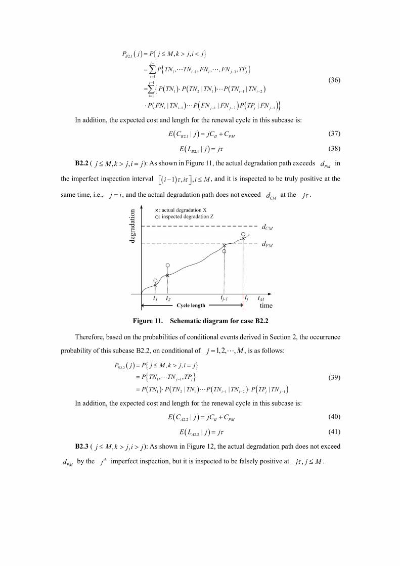
Figure 2. Schematic diagram for case A1.1

A1.1 ( ): As shown in Figure 2, the actual degradation path exceeds both and

in the same time interval , and the inspected degradation does not exceed

by the inspection.

Therefore, based on the probabilities of conditional events derived in Section 2, the occurrence

probability of this subcase A1.1, on conditional of , is as follows:

(9)

In addition, the expected cost and length for the renewal cycle in this subcase is:

(10)

(11)

A1.2 ( ): As shown in Figure 3, the actual degradation path exceeds in the time

interval , but this is not inspected to be truly positive by the inspection.

Besides, the actual degradation path exceeds in the time interval .

Note that in this subcase, the condition that and the primary constraint that

together leads to the constraint that .

j k³

,j k i k³ = PMd

CMd ( )1 ,k kt t-é ùë û PMd

( )1 thk -

( )0,FT Î +¥

( ) { }{ }( ) ( ) ( ) ( )

1.1

1 2 1

1 2 1 1 2 1

,

, , , ,

| | |

A F

k k CM

k k k CM k

P T P j k i k

P TN TN TN X d

P TN P TN TN P TN TN P X d TN-

- - -

= ³ =

= ³

= × × ³

!

!

( ) ( )1.1| 1A F II CME C T k C C= - +

( )1.1 |A F FE L T T=

,j k i k³ < PMd

( )1 ,i it t-é ùë û ( )1 ,thk k i- >

CMd ( )1 ,k kt t-é ùë û

,j k i k³ <

1 i k£ £ 1k >




(12)


(13)

(14)

Case A2: The cycle ends up with PM.

In this case, failure occurs after the inspection time when it is inspected to conduct PM,

i.e., . Considering that FNs or FP may happen for the imperfect inspections, this case can be

further divided into three subcases:


interval , but it is not inspected to be truly positive until the inspection. Also,

the actual degradation path does not exceed at the inspection.



( )0,FT Î +¥

( ) { }

{ }

( ) ( ) ( ){ ( )

( ) ( ) ( )}

1.2

1

1 1 111

1 2 1 1 2 11

1 1 2 1

,

, , , , , ,

| | |

| | |

A F

k

i i k k CMik

i i i ii

i i k k k CM k

P T P j k i k

P TN TN FN FN X d

P TN P TN TN P TN TN P FN TN

P FN FN P FN FN P X d FN

-

- -=

-

- - -=

+ - - -

= ³ <

= ³

= × ×

× × ³

å

å

! !

!

!

( ) ( )1.2| 1A F II CME C T k C C= - +

( )1.2 |A F FE L T T=

thj

k j>

,k j i j> < PMd

( )1 ,i it t-é ùë û ,thj j i>

CMdthj

,k j i j> <

1 i k£ £ 1j >




(15)


(16)

(17)


interval , and it is inspected to be truly positive at the same inspection time, i.e., .

Also, the actual degradation path does not exceed at the inspection.




1,2, ,j = +¥!

( ) { }

{ }

( ) ( ) ( ){

( ) ( ) ( )}

2.1

1

1 1 111

1 2 1 1 21

1 1 2 1

,

, , , , ,

| |

| | |

A

j

i i j jij

i ii

i i j j j j

P j P k j i j

P TN TN FN FN TP

P TN P TN TN P TN TN

P FN TN P FN FN P TP FN

-

- -=

-

- -=

- - - -

= > <

=

= ×

×

å

å

! !

!

!

( )2.1 |A II PME C j jC C= +

( )2.1 |AE L j jt=

,k j i j> = PMd

( )1 ,i it t-é ùë û j i=

CMdthj

1,2, ,j = +¥!

(18)


(19)

(20)

A2.3 ( ): As shown in Figure 6, the actual degradation path does not exceed

by the inspection, but it is inspected to be falsely positive at .




(21)


(22)

(23)

Total maintenance cost of policy :

To account for the total long run cost rate for the proposed policy , first we have to verify

that the above cases and subcases are mutually exclusive events. In fact, we believe that this condition

holds because is the number of the first inspection after the actual degradation path exceeds ,

is the number of the first inspection after the inspected degradation path exceeds , and is the

number of the first inspection after the actual degradation path exceeds . Considering that the above

subcases involves different relationships of size between variables , and that there is no repetitive

( ) { }{ }( ) ( ) ( ) ( )

2.2

1 1

1 2 1 1 2 1

,

, ,

| | |

A

j j

i i j j

P j P k j i j

P TN TN TP

P TN P TN TN P TN TN P TP TN

-

- - -

= > =

=

= × ×

!

!

( )2.2 |A II PME C j jC C= +

( )2.2 |AE L j jt=

,k j i j> > PMdthj jt

1,2, ,j = +¥!

( ) { }{ }( ) ( ) ( ) ( )

3.3

1 1

1 2 1 1 2 1

,

= , ,

| | |

A

j j

i i j j

P j P k j i j

P TN TN FP

P TN P TN TN P TN TN P FP TN

-

- - -

= > >

= × ×

!

!

( )2.3 |A II PME C j jC C= +

( )2.3 |AE L j jt=

AS

AS

i PMd

j CMd k

CMd

, ,i j k

situation in any two subcases, subcases A1.1, A.1.2, A2.1, A.2.2, and A.2.3 are believed to be mutually

exclusive events.

Furthermore, the above subcases compose the whole events of maintenance policy becasuse

that the sum of the occurrence probabilities of cases A1 and A2 is:

where because that the fact leads to a primary constraint that

, that is to say the case won’t occur and .

In summary, by considering the distribution characteristic of system failure time and all

possible values of the inspection number to conduct PM, and summing over all the above cases

and subcases, we can obtain the expected cost and length for as Equations (24) and (25).

Therefore, its long run cost rate for policy can be formulated by the ratio of and

, and the optimal and for can be designed through minimizing .

(24)

(25)

where is the CDF of the system failure time :

(26)

3.2.2 Cost analysis for the maintenance policy with two-stage inspection scheme

Similar to , policy is also with fixed inspection interval . Besides, its renewal cycle

may also end up with either CM or PM, and the cycle termination can lie in either the perfect-

inspection stage or the imperfect-inspection stage. Therefore, we derive the occurrence probability,

the expected length and cost for the renewal cycle of in the following cases. Denotations

are the same with those in subsection 3.2.1. The optimization variables for policy

AS

{ } { } { } { } { }{ } { } { }

{ }

1 2

1.1 1.2 2.1 2.2 2.3

, , , , ,

,

1 ,1

A A

A A A A A

P PP P P P PP j k i k P j k i k P k j i j P k j i j P k j i j

P j k P j k i k P k j

P j k i k

+= + + + +

= ³ = + ³ < + > < + > = + > >

= ³ - ³ > + >

= - ³ >

=

{ }, 0P j k i k³ > = 0 PM CMd d< £

1 1 1PM CMi d j dt t£ = + £ = +ê úê úë û ë û i k> ( ) 0P i k> =

FT

j

AS

ACR AS ( )AE C

( )AE L t PMd AS ACR

( ) ( ) ( ) ( ) ( ) ( )

( ) ( ) ( ) ( ) ( )

( ) ( ) ( ) ( ) ( ) ( )

1 1 2 201

1.1 1.1 1.2 1.20

2.1 2.1 2.2 2.2 2.3 2.31

| |

| |

| | |

A A F A F T A Aj

A F A F A F A F T

A A A A A Aj

E C E C T P T d F t E C j P j

E C T P T E C T P T d F t

E C j P j E C j P j E C j P j

+¥+¥

=

+¥

+¥

=

= × + ×é ùë û

= × + ×é ù é ùë û ë û

+ × + × + ×é ùë û

åò

ò

å

( ) ( ) ( ) ( ) ( ) ( )

( ) ( ) ( ) ( ) ( )

( ) ( ) ( ) ( ) ( ) ( )

1 1 2 201

1.1 1.1 1.2 1.20

2.1 2.1 2.2 2.2 2.3 2.31

| |

| |

| | |

A A F A F T A Aj

A F A F A F A F T

A A A A A Aj

E L E L T P T d F t E L j P j

E L T P T E L T P T d F t

E L j P j E L j P j E L j P j

+¥+¥

=

+¥

+¥

=

= × + ×é ùë û

= × + ×é ù é ùë û ë û

+ × + × + ×é ùë û

åò

ò

å

( )TF t FT

( ) { } ( ){ } ( );F F CM X CMF t P T t P X t d F d t= < = > =

AS BS t

BS

, , , Fi j k T BS

include inspection interval , preventive maintenance threshold level and number of

inspections for stage transition.

Case B1: The cycle ends up with CM.

In this case, failure occurs before the inspection time when it is inspected to conduct PM,

i.e., . Considering that FNs may happen for the imperfect inspections before failure, and that

the last inspection of the cycle may be either imperfect or perfect, this case can be further divided

into three subcases:

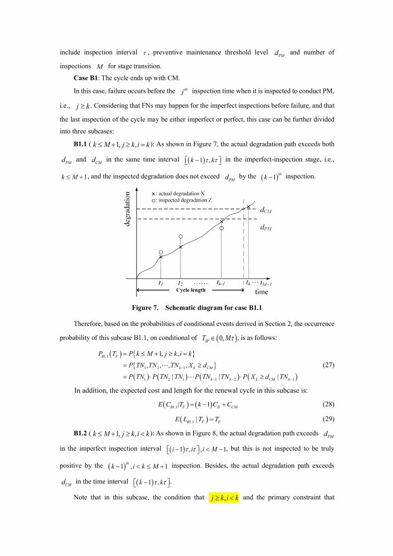
B1.1 ( ): As shown in Figure 7, the actual degradation path exceeds both

and in the same time interval in the imperfect-inspection stage, i.e.,

, and the inspected degradation does not exceed by the inspection.

Figure 7. Schematic diagram for case B1.1


probability of this subcase B1.1, on conditional of , is as follows:

(27)


(28)

(29)

B1.2 ( ): As shown in Figure 8, the actual degradation path exceeds

in the imperfect inspection interval , but this is not inspected to be truly

positive by the inspection. Besides, the actual degradation path exceeds

in the time interval .


t PMd

M

thj

j k³

1, ,k M j k i k£ + ³ =

PMd CMd ( )1 ,k kt t-é ùë û

1k M£ + PMd ( )1 thk -

( )0,SFT MtÎ

( ) { }{ }( ) ( ) ( ) ( )

1.1

1 2 1

1 2 1 1 2 1

1, ,

, , , ,

| | |

B F

k k CM

k k k CM k

P T P k M j k i k

P TN TN TN X d

P TN P TN TN P TN TN P X d TN-

- - -

= £ + ³ =

= ³

= × × ³

!

!

( ) ( )1.1| 1B F II CME C T k C C= - +

( )1.1 |B F FE L T T=

1, ,k M j k i k£ + ³ < PMd

( )1 , , 1i i i Mt t- < -é ùë û

( )1 , 1thk i k M- < £ +

CMd ( )1 ,k kt t-é ùë û

,j k i k³ <





(30)


(31)

(32)

B1.3 ( ): As shown in Figure 9, the actual degradation path exceeds in

the perfect inspection interval , which leads to the fact that the actual and

perfectly inspected degradation path exceeds in the same inspection interval, i.e., ,

because if or , then PM will be conducted before the system fails.


1 i k£ £ 1k >

( )0,FT MtÎ

( ) { }

{ }

( ) ( ) ( ){ ( )

( ) ( ) ( )}

1.2

1

1 1 111

1 2 1 1 2 11

1 1 2 1

1, ,

= , , , , , ,

| | |

| | |

B F

k

i i k k CMik

i i i ii

i i k k k CM k

P T P k M j k i k

P TN TN FN FN X d

P TN P TN TN P TN TN P FN TN

P FN FN P FN FN P X d FN

-

- -=

-

- - -=

+ - - -

= £ + ³ <

³

= × ×

× × ³

å

å

! !

!

!

( ) ( )1.2| 1B F II CME C T k C C= - +

( )1.2 |B F FE L T T=

1,k M i j k> + = = CMd

( )1 , , 1k k k Mt t- > +é ùë û

PMd i j k= =

i k< j k<



(33)


(34)

(35)

Case B2: The cycle ends up with inspected PM.

In this case, failure occurs after the inspection time when it is inspected to conduct PM,

i.e., . Considering that FNs or FP may happen for the imperfect inspections, and that the last

inspection of the cycle may be either imperfect or perfect, this case can be divided into four subcases:


in the imperfect inspection interval , but it is not inspected to be truly positive

until the imperfect inspection. Also, the actual degradation path does not exceed

at the inspection.






( )0,FT MtÎ

{ }{ }( ) ( ) ( )( ) ( )

1.3

1 1

1 2 1 1

1 1

1,

, , , ,

| |

| |

B

M k PM k CM

M M

k PM M k CM k PM

P P k M i j k

P TN TN X d X d


P X d TN P X d X d

-

-

- -

= > + = =

= < ³

= ×

× < × ³ <

!

!

( ) ( )1.3| 1B F II PI CME C T MC k M C C= + - - +

( )1.3 |B F FE L T T=

thj

k j>

, ,j M k j i j£ > < PMd

( )1 , ,i i i Mt t- <é ùë û

,thj i j M< £

CMdthj

,k j i j> <

1 i k£ £ 1j >

1,2, ,j M= !

(36)


(37)

(38)

B2.2 ( ): As shown in Figure 11, the actual degradation path exceeds in

the imperfect inspection interval , and it is inspected to be truly positive at the

same time, i.e., , and the actual degradation path does not exceed at the .




(39)


(40)

(41)

B2.3 ( ): As shown in Figure 12, the actual degradation path does not exceed

by the imperfect inspection, but it is inspected to be falsely positive at .

( ) { }

{ }

( ) ( ) ( ){

( ) ( ) ( )}

2.1

1

1 1 111

1 2 1 1 21

1 1 2 1

, ,

, , , , ,

= | |

| | |

B

j

i i j jij

i ii

i i j j j j

P j P j M k j i j

P TN TN FN FN TP


P FN TN P FN FN P TP FN

-

- -=

-

- -=

- - - -

= £ > <

=

×

×

å

å

! !

!

!

( )2.1 |B II PME C j jC C= +

( )2.1 |BE L j jt=

, ,j M k j i j£ > = PMd

( )1 , ,i i i Mt t- £é ùë û

j i= CMd jt

1,2, ,j M= !

( ) { }{ }( ) ( ) ( ) ( )

2.2

1 1

1 2 1 1 2 1

, ,

, ,

| | |

B

j j

i i j j

P j P j M k j i j

P TN TN TP

P TN P TN TN P TN TN P TP TN

-

- - -

= £ > =

=

= × ×

!

!

( )2.2 |A II PME C j jC C= +

( )2.2 |AE L j jt=

, ,j M k j i j£ > >

PMdthj ,j j Mt £




(42)


(43)

(44)


in the perfect inspection interval , and it is inspected to be truly positive at

the same time. Also, the actual degradation path does not exceed at the inspection.




1,2, ,j M= !

( ) { }{ }( ) ( ) ( ) ( )

2.3

1 1

1 2 1 1 2 1

, ,

, ,

| | |

B

j j

i i j j

P j P j M k j i j

P TN TN FP

P TN P TN TN P TN TN P FP TN

-

- - -

= £ > >

=

= × ×

!

!

( )2.3 |A II PME C j jC C= +

( )2.3 |AE L j jt=

1, ,j M k j i j³ + > = PMd

( )1 , , 1i i i Mt t- ³ +é ùë û

CMdthj

1, 2, ,j M M= + + +¥!

(45)


(46)

(47)

Total maintenance cost of policy :

To account for the total long run cost rate for the proposed policy , first we have to verify

that the above cases and subcases are mutually exclusive events. Similar to the situation of policy

, the subcases B1.1, B.1.2, B.1.3, B2.1, B.2.2, B.2.3 and B.2.4 involves different relationships of

size between variables , and that there is no repetitive situation in any two subcases.

Therefore, these subcases are believed to be mutually exclusive events.

Furthermore, the above subcases compose the whole events of maintenance policy

becasuse that the sum of the occurrence probabilities of cases B1 and B2 is:

where

(1) because the case won’t occur and ;

(2) When , at the perfect inspection, the actual degradation level (equals to the

inspected degradation level) is larger than both and , that is to say can’t be larger than

and ;

(3) When , at the perfect inspection, the actual degradation level (equals to

the inspected degradation level) firstly exceeds both and , that is to say equals to and

;

(4) When , at the perfect inspection, the actual degradation level equals to the

inspected degradation level and both firstly exceeds , that is to say equals to and

;

{ }{ }( ) ( ) ( )( ) ( )

2.4

1 1

1 2 1 1

1 1

1, ,

= , , ,

| |

| |

B

M j PM PM j CM

M M

j PM M PM j CM j PM

P P j M k j i j

P TN TN X d d X d


P X d TN P d X d X d

-

-

- -

= ³ + > =

< £ <

= ×

× < × £ < <

!

!

( ) ( )2.4 |A II PI PME C j MC j M C C= + - +

( )2.4 |AE L j jt=

BS

BS

BS

, , ,i j k M

BS

{ } { } { }{ } { } { } { }{ } { } { } { }

1 2

1.1 1.2 1.3 2.1 2.2 2.3 2.4

1, , 1, , 1,

, , , , , , 1, ,

1, 1, , 1, 1,

B B

B B B B B B B

P PP P P P P P PP k M j k i k P k M j k i k P k M i j k

P j M k j i j P j M k j i j P j M k j i j P j M k j i j

P k M j k P k M j k i k P k M j k P k M j k

P k M

+= + + + + + +

= £ + ³ = + £ + ³ < + > + = =

+ £ > < + £ > = + £ > > + ³ + > =

= £ + ³ - £ + ³ > + > + ³ - > + >

- > +{ } { } { } { }{ } { } { } { }{ } { }

1, , , + 1, 1, ,

1, , 1, 1, ,

1, ,1

j k i k P j M k j P j M k j P j M k j i j

P j k P k M j k i k P k M j k P k M j k i k

P k j P j M k j i j

= ¹ + £ > ³ + > - ³ + > ¹

= ³ - £ + ³ > + > + > + > + = ¹é ùë û+ > - ³ + > ¹

=

{ }1, , 0P k M j k i k£ + ³ > = i k> ( ) 0P i k> =

1k M> + thk

PMd CMd j

k { }1, 0P k M j k> + > =

1,k M j k> + = thk

PMd CMd i k

{ }1, , 0P k M j k i k> + = ¹ =

1,j M k j³ + > thj

PMd i j

{ }1, , 0P j M k j i j³ + > ¹ =

In summary, by considering the distribution characteristic of system failure time and all

possible values of the inspection number to conduct PM, and by summing over all the above cases

and subcases, we can obtain the expected cost and length for policy as Equations (48) and (49).

Therefore, the long run cost rate for policy can be formulated by the ratio of and

, and the optimal , and for can be designed through minimizing .

(48)

(49)

where is also the CDF of the system failure time , and can be referred to equation (26).

4 Performance evaluation of the proposed policies In this section, we implement the two considered maintenance policies through numerical

experiments and a real case study, and also illustrate their advantages over the classical maintenance

policy with perfect inspections.

4.1 Numerical experiments

First, under the formulations of degradation model and maintenance policy in Section 2, we

use a nonlinear gamma degradation process for illustration, and the other

model and cost parameters are assumed to be , , , ,

and . Utilizing an iterated grid search (IGS) approach [45], optimization variables for

policies and are obtained based on the cost analysis results in Sections 3.1 and 3.2,

respectively. Then according to their optimal long run cost rate, the two policies are compared to

the classical maintenance policy , and their advantages are illustrated based on sensitivity

FT

j

BS

BCR BS ( )BE C

( )BE L t PMd M BS BCR

( ) ( ) ( ) ( ) ( ) ( )

( ) ( ) ( ) ( ) ( )

( ) ( ) ( )

( ) ( ) ( ) ( ) ( ) ( )

( )

1 1 2 201

1.1 1.1 1.2 1.20

1.3 1.3

2.1 2.1 2.2 2.2 2.3 2.31

2.4

| |

| |

|

| | |

|

B B F B F T B Bj

M

B F B F B F B F T

B F B F TMM

B B B B B Bj

B

E C E C T P T d F t E C j P j

E C T P T E C T P T d F t

E C T P T d F t

E C j P j E C j P j E C j P j

E C j

t

t

+¥+¥

=

+¥

=

= × + ×é ùë û

= × + ×é ù é ùë û ë û

+ ×é ù é ùë û ë û

+ × + × + ×é ùë û

+

åò

òò

å

( )2.41

Bj M

P j+¥

= +

×é ùë ûå

( ) ( ) ( ) ( ) ( ) ( )

( ) ( ) ( ) ( ) ( )

( ) ( ) ( )

( ) ( ) ( ) ( ) ( ) ( )

( )

1 1 2 201

1.1 1.1 1.2 1.20

1.3 1.3

2.1 2.1 2.2 2.2 2.3 2.31

2.4

| |

| |

|

| | |

|

B B F B F T B Bj

M

B F B F B F B F T

B F B F TMM

B B B B B Bj

B

E L E L T P T d F t E L j P j

E L T P T E L T P T d F t

E L T P T d F t

E L j P j E L j P j E L j P j

E L j

t

t

+¥+¥

=

+¥

=

= × + ×é ùë û

= × + ×é ù é ùë û ë û

+ ×é ù é ùë û ë û

+ × + × + ×é ùë û

+

åò

òò

å

( )2.41

Bj M

P j+¥

= +

×é ùë ûå

( )TF t FT

1.2(1.5 ,1.5)Gamma t×

2es = 1IIC = 3PIC = 30PMC = 80CMC =

10CMd =

AS BS

0S

analysis on the cost parameter, the variation of the degradation process and the measurement error.

For the proposed maintenance policy with imperfect inspections, we compute its long run

cost rate , and plot the three-dimensional surface and the iso-level curve for with respect

to and , as shown in Figure 14, where the discretization steps of and

are respectively 0.01 and 0.1. The surface is shown to be convex, which indicates that there is

a global optimal combination of inspection and maintenance policy, i.e., and ,

corresponding to the minimum long run cost rate . Furthermore, to increase the

credibility of Figure 14, we fix one of the two variables , and present the values of

with respect to the other variable, as shown in Table 2 and Table 3.

Figure 14. Long run cost rate with respect to

Table 2. Long run cost rate with respect to under fixed

1.45 1.46 1.47 1.48 1.49 1.50 1.51 1.52 1.53 1.54 1.55 7.557 7.552 7.543 7.539 7.537 7.534 7.535 7.536 7.538 7.540 7.542


6 6.1 6.2 6.3 6.4 6.5 6.6 6.7 6.8 6.9 7 7.56 7.54 7.53 7.54 7.54 7.56 7.57 7.59 7.62 7.65 7.69

For the proposed maintenance policy with two-stage inspection scheme, its long run cost

rate can be obtained by the ratio of and . By computing under

different values of , and , the minimum long run cost rate is found to be ,

corresponding to the optimization variables , and . Furthermore, to

visually show how changes with , and , we fix to be its optimal value 4,

and plot the three-dimensional surface for with respect to and ,

where the discretization steps of and are respectively 0.01 and 0.1. Besides, the values of

AS

ACR ACR

[ ]1,2t Î [ ]5,8PMd Î t

PMd

1.50t = 6.2PMd =

,min 7.53ACR =

, PMdt ACR

ACR , PMdt

ACR t 6.2PMd =

t

BCR

ACR PMd 1.50t =

PMd

BCR

BS

BCR ( )BE C ( )BE L BCR

t PMd M B,min 7.42CR =

1.47t = 6.5PMd = 4M =

BCR t PMd M M

BCR [ ]1,2t Î [ ]5.5,8PMd Î

t PMd

with respect to one of the two variables , by fixing the other variable, are presented in

Table 4 and Table 5. Similar to the plot of in Figure 14, the surface for in Figure 15 is

also convex, indicating the existence of global optimization for policy .


1.40 1.41 1.42 1.43 1.44 1.45 1.46 1.47 1.48 1.49 1.50 7.434 7.432 7.429 7.427 7.425 7.422 7.420 7.421 7.423 7.425 7.427


6 6.1 6.2 6.3 6.4 6.5 6.6 6.7 6.8 6.9 7 7.52 7.49 7.47 7.45 7.43 7.42 7.43 7.43 7.44 7.44 7.47

Figure 15. Long run cost rate with respect to under fixed

In addition, under fixed and , the values of with respect to

is provided in Table 6, and the changing curve is plotted in Figure 16, where the

discretization steps of is 1. It can be seen that decreases when increases from 1 to

4, then increases with and finally converges to when is larger than 6, which is

because that for the system under maintenance policy with large enough , the occurrence

of failure will be earlier than the shifting time of the inspections from imperfect ones to perfect ones,

and the system maintenance will have nothing to do with .


1 2 3 4 5 6 7 8 9 10 7.99 7.68 7.49 7.42 7.51 7.56 7.57 7.57 7.57 7.57

BCR , PMdt

ACR BCR

BS

BCR t 6.5, 4PMd M= =

t

BCR

BCR PMd 1.47, 4Mt = =

PMd

BCR

BCR , PMdt 4M =

1.47t = 6.5PMd = BCR

[ ]1,10M Î

M BCR M

M 7.57 M

BS M

M

BCR M 1.47, 6.5PMdt = =

M

BCR

Figure 16. Long run cost rate with respect to under fixed

4.2 Sensitivity analysis

Based on different perfect inspection cost , the optimal long run cost rates of the three

policies are plotted in Figure 17. It can be shown that with the increase of , the optimal cost rate

of policies and rise obviously, while policy is not affected. The curves for policies

and cross at a point corresponding to when perfect inspections are not too cheap and

is higher than about 2.6, will be more economical than . Besides, for all values of ,

policy is always the best choice in that it approaches the curve of when is low, and

converges to when is high.

Figure 17. Sensitivity analysis of the optimal maintenance cost rate to

In addition, we also investigate the effect of PM and CM cost on the maintenance policies, as

shown in Figures 18 and 19, respectively. It can be seen that as or increases, the curves

of all three policies show obvious rising trends, and in an economical viewpoint, policy is

always the best and is the worst. Besides, the sensitivity on is larger than that on ,

which is because that all three CBM strategies are meant to prevent the occurrence of failures,

therefore is less influenced by the cost incurred by CM activities against failures.

BCR M 1.47, 6.5PMdt = =

PIC

PIC

0S BS AS

0S AS PIC

AS 0S PIC

BS 0S PIC

AS PIC

PIC

PMC CMC

BS

0S PMC CMC



Additionally, considering that the variation of the degradation process and the measurement

error can affect the maintenance policies, we plot the sensitivity analysis of the optimal maintenance

cost rate to and in Figures 20 and 21. Firstly, in order to keep the comparability of policies

with different values of , we fix the form of nonlinear drift function and the mean

function of the degradation process . Under this circumstance, if we increase the value of

, we also have to incarease that of proportionally, and this will lead to smaller variation of

the degradation process, i.e., , and decrease the optimal cost rates for all the three policies,

although in different rates. Besides, the increase of will make it harder to prevent the

occurrence of failure, and result in higher cost rates for policies and . For the comparison

among the three policies, we can see that policy still has the best economic performance for all

values of and , and policy turns to be worse than when is smaller than about

2.2, or when exceeds around 2.25.

PMC

CMC

a es

a ( )tL

( )tabL

a b

( )2 tab

L

es

AS BS

BS

a es 0S AS a

es


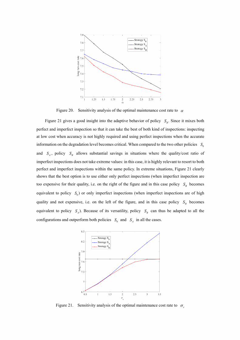
Figure 21 gives a good insight into the adaptive behavior of policy . Since it mixes both

perfect and imperfect inspection so that it can take the best of both kind of inspections: inspecting

at low cost when accuracy is not highly required and using perfect inspections when the accurate

information on the degradation level becomes critical. When compared to the two other policies

and , policy allows substantial savings in situations where the quality/cost ratio of

imperfect inspections does not take extreme values: in this case, it is highly relevant to resort to both

perfect and imperfect inspections within the same policy. In extreme situations, Figure 21 clearly

shows that the best option is to use either only perfect inspections (when imperfect inspection are

too expensive for their quality, i.e. on the right of the figure and in this case policy becomes

equivalent to policy ) or only imperfect inspections (when imperfect inspections are of high

quality and not expensive, i.e. on the left of the figure, and in this case policy becomes

equivalent to policy ). Because of its versatility, policy can thus be adapted to all the

configurations and outperform both policies and in all the cases.


a

BS

0S

AS BS

BS

0S

BS

AS BS

0S AS

es

4.3 Robustness Analysis

It should be noted that the above analysis is all based on the assumption of an accurate

knowledge about inspection quality. However, in practice we may mis-specify the model

assumptions, e.g. on whether the inspections are perfect or not, and on the exact value of the variance

of measurement errors. Therefore, we analyze the robustness of the three maintenance policies by

studying the effect of inspection quality mis-specification. In Tables 7-9, the optimal long run cost

rates are evaluated by implementing on a system with the measurement error standard deviation at

its true value, and the maintenance policies as well as decision variables optimized for wrongly

specified .

As the deviation between the true and wrongly specified increases, the optimal long run

cost rates for the three policies all increase. Besides, the proposed policies and are always

better than the classical policy for all true and wrongly specified . For the comparison

between and , it can be indicated that when the true is bigger than the wrongly

specified , i.e., when we overestimate the measurement instrument performance and

underestimate the measurement error, then it is more beneficial to adopt the maintenance policy .

When the true is smaller than the wrongly specified , i.e., when we underestimate the

measurement instrument performance and overestimate the size of measurement error, then

maintenance policy is more preferable from an economic point of view. One of the interesting

conclusion of this analysis is about the robustness of the proposed policies and : even if a

wrong value of the measurement error variance is used to optimize these policies, they are robust

enough so that their performance remains better than the policy that assumes wrongly perfect

inspections.

Table 7. Optimal long run cost rate for mis-specified policy

Wrongly specified True

0

0.5 7.68 1 7.76

1.5 7.94 2 8.22

2.5 8.52 3 8.81

3.5 9.06



0.5 1 1.5 2 2.5 3 3.5

0.5 6.74 6.75 6.76 6.75 6.76 6.78 6.79

es

es

es

AS BS

0S es

AS BS es

es

BS

es es

AS

AS BS

0S

0S

es

es

AS

es

es

1 6.95 6.94 6.94 6.95 6.96 7.01 7.01 1.5 7.23 7.22 7.21 7.22 7.25 7.29 7.29 2 7.54 7.54 7.53 7.53 7.55 7.59 7.60

2.5 7.89 7.89 7.88 7.87 7.86 7.89 7.90 3 8.21 8.2 8.22 8.2 8.2 8.17 8.19

3.5 8.53 8.51 8.54 8.49 8.51 8.46 8.44



0.5 1 1.5 2 2.5 3 3.5

0.5 6.74 6.75 6.76 7.00 7.25 7.67 7.68 1 6.95 6.94 6.95 7.10 7.29 7.67 7.68

1.5 7.23 7.22 7.20 7.25 7.35 7.67 7.68 2 7.53 7.53 7.52 7.32 7.45 7.67 7.68

2.5 7.86 7.87 7.87 7.65 7.59 7.67 7.68 3 8.19 8.19 8.18 7.88 7.78 7.67 7.68

3.5 8.50 8.51 8.52 8.12 7.96 7.67 7.68

4.4 Case study

In order to show how the presented maintenance policies can be used in practical applications,

we apply them to a “three-bladed rotor system” on an offshore wind turbine. A blade is an important

part of a wind turbine, and its failure is caused by residual strength reduction due to crack growth

[46]. In fact, cracks on blades are usually monitored by periodic inspections, but such crack length

measurements by imperfect inspection systems are often contaminated by errors [47]. Therefore,

this case study is intended to implement the two proposed maintenance policies with imperfect

inspections, and to see which policy offers the best benefit.

The dataset used in this study is referred to some relevant references [48,49]. The blade crack

growth process can be modelled by a homogeneous gamma process with shape and scale parameters

given by cm/month and . Therefore, the mean degradation rate will be

cm/month. In addition, the failure threshold level for the blade crack length is

cm. For the imperfectly inspected crack length, the variation of the measurement error is

cm. As for the cost for the blades, the cost for each perfect inspection is €, the

cost for each imperfect inspection is €, the Cost of performing a corrective maintenance

is €, and the Cost of performing a preventive maintenance is €.

Also utilizing an iterated grid search (IGS) approach, we obtain optimization variables for the

classical maintenance policy , the proposed maintenance policies and , respevtively.

Table 10 lists the values of , , as well as the the corresponding long run cost rate and

the percentage reduction of policies and compared to policy . It can be indicated that

for the “three-bladed rotor system” on an offshore wind turbine, making maintenance decisions with

BS

es

es

0.542a = 1.147b =

0.4725a b =

20CMd =

1es = 3000PIC =

2000IIC =

440400CMC = 225000PMC =

0S AS BS

t PMd M

AS BS 0S

imperfect inspections allows substantial savings than making decisions with perfect ones, and it is

more economically beneficial to mix both perfect and imperfect inspections, and adapt the more

flexible maintenance policy .

Table 10. A comparison between the three maintenance policies for the blade case

Maintenance policy

optimal (month)

optimal (cm)

optimal

Minimum long run cost rate(€/month)

Cost reduction compared to pocily

6.2 16 - 6980.20 0

5.7 16 - 6918.97 0.88%

5.3 16 6 6881.87 1.41%

Furthermore, to account for other potential crack length inspection systems, we analyze the

most economical maintenance policy in different cases of imperfect inspection cost and

variation of measurement error, and list the corresponding minimum long run cost rates in Table 11.

It can be indicated that compared to the case with medium values of and , the economic

performance is better in the case with lower imperfect inspection cost and larger measurement error.

Therefore, the wind turbine operators are advised to make more efforts on decreasing the cost of an

imperfect inspection system, even by paying the price of inspection quality.

Table 11. A comparison for maintenance policy with different values of and

Imperfect inspection cost (€)

Variation of measurement error

(cm)

Minimum long run cost rate(€/month)

Cost reduction compared to pocily

2000 1 6881.87 1.41% 1800 1.1 6845.37 1.93% 2200 0.9 6899.31 1.16%

5 Conclusion Considering the measurement errors for the inspections of continuous degradation processes,

this paper proposes two CBM policies and . Maintenance decisions of them are

respectively made upon a purely imperfect inspection scheme and a two-stage inspection scheme,

i.e., to shift from imperfect inspections to perfect ones after inspections. To calculate the long

run cost rates of the two policies, we derive the occurrence probabilities of conditional events

concerning TP, TN, FP and FN, and compute the occurrence probabilities, expected cost and length

for the renewal cycle in different cases. The two policies are implemented through some numerical

experiments, and sensitivity analysis shows that the proposed policy is more economical than

the classical one on the condition that the perfect inspection cost is not too low, variation of the

degradation process is not too small or the size of measurement error is not too large. Besides, thanks

to the generalization introduced by two-stage inspection scheme, the proposed policy always

has the best economic performance among the three maintenance policies, and is recommended to

be chosen in practice. In addition, by analyzing the effect of inspection quality mis-specification on

BS

tPMd M

0S

0S

AS

BS

BS

IIC es

BS IIC es

IIC es0S

AS BS

M

AS

0S

BS

the maintenance policies, the proposed policies and are found to be more robust than .

Furthermore, a real case study of a “three-bladed rotor system” on an offshore wind turbine is

presented to show how the proposed maintenance policies can be used in practical applications.

Our model and our results can give some insight on how different kinds of inspections, each

with different quality and different costs, should be optimally used and sequenced to take the most

benefit of them. once implemented within computer-aided maintenance management system, our

proposed model would be hence of interest to maintenance decision-makers: as a stationary control

limit rule, the proposed model is easy to implement. Besides, the mixture of perfect and imperfect

inspections lead to an most beneficial system monitoring, and the amount of cost savings obviously

depend on the different costs of the different maintenance actions, inspections and on the different

features of the maintenance actions and inspections available for a given maintained system.

The model of imperfect inspection could be further improved in several ways, which opens

several research perspectives. Firstly, the dependence between the variance of the inspection noise

and the measured deterioration level should be considered to make the maintenance policy more

realistic. Besides, the proposed model can be generalized by taking into account imperfect

maintenance activities. Furthermore, another interesting work can be the issue of maintenance

decision-making using different inspections with different quality and cost characteristics.

Acknowledgement This work was supported by the National Natural Science Foundation of China under Grant

71672006, the Grant JSZL2017601B006, and the Fundamental Research Funds for the Central

Universities under Grant No. YWF-19-BJ-J-160.

References [1] A.F. Shahraki, O.P. Yadav, H. Liao, A Review on Degradation Modelling and Its

Engineering Applications, Int. J. Perform. Eng. 13 (2017) 299–314. [2] D.S. González-González, R.J. Praga-Alejo, M. Cantú-Sifuentes, A non-linear fuzzy

degradation model for estimating reliability of a polymeric coating, Appl. Math. Model. 40 (2016) 1387–1401. https://doi.org/10.1016/j.apm.2015.06.033.

[3] Z.-S. Ye, M. Xie, Stochastic modelling and analysis of degradation for highly reliable products, Appl. Stoch. Models Bus. Ind. 31 (2015) 16–32. https://doi.org/10.1002/asmb.2063.

[4] D. Pan, J.-B. Liu, F. Huang, J. Cao, A. Alsaedi, A Wiener process model with truncated normal distribution for reliability analysis, Appl. Math. Model. 50 (2017) 333–346. https://doi.org/10.1016/j.apm.2017.05.049.

[5] S. Hao, J. Yang, C. Berenguer, Nonlinear step-stress accelerated degradation modelling considering three sources of variability, Reliab. Eng. Syst. Saf. 172 (2018) 207–215. https://doi.org/10.1016/j.ress.2017.12.012.

[6] G. Pulcini, A perturbed gamma process with statistically dependent measurement errors, Reliab. Eng. Syst. Saf. 152 (2016) 296–306. https://doi.org/10.1016/j.ress.2016.03.024.

[7] C. Paroissin, Online Estimation Methods for the Gamma Degradation Process, IEEE Trans. Reliab. 66 (2017) 1361–1367. https://doi.org/10.1109/TR.2017.2757768.

[8] D. He, Y. Wang, G. Chang, Objective Bayesian analysis for the accelerated degradation model based on the inverse Gaussian process, Appl. Math. Model. 61 (2018) 341–350. https://doi.org/10.1016/j.apm.2018.04.025.

[9] J. Guo, C. Wang, J. Cabrera, E.A. Elsayed, Improved inverse Gaussian process and bootstrap: Degradation and reliability metrics, Reliab. Eng. Syst. Saf. 178 (2018) 269–277.

AS BS 0S

https://doi.org/10.1016/j.ress.2018.06.013. [10] A. Grall, C. Bérenguer, L. Dieulle, A condition-based maintenance policy for

stochastically deteriorating systems, Reliab. Eng. Syst. Saf. 76 (2002) 167–180. https://doi.org/10.1016/S0951-8320(01)00148-X.

[11] B. de Jonge, R. Teunter, T. Tinga, The influence of practical factors on the benefits of condition-based maintenance over time-based maintenance, Reliab. Eng. Syst. Saf. 158 (2017) 21–30. https://doi.org/10.1016/j.ress.2016.10.002.

[12] R. Ahmad, S. Kamaruddin, An overview of time-based and condition-based maintenance in industrial application, Comput. Ind. Eng. 63 (2012) 135–149. https://doi.org/10.1016/j.cie.2012.02.002.

[13] J.M. van Noortwijk, A survey of the application of gamma processes in maintenance, Reliab. Eng. Syst. Saf. 94 (2009) 2–21. https://doi.org/10.1016/j.ress.2007.03.019.

[14] S. Alaswad, Y. Xiang, A review on condition-based maintenance optimization models for stochastically deteriorating system, Reliab. Eng. Syst. Saf. 157 (2017) 54–63. https://doi.org/10.1016/j.ress.2016.08.009.

[15] Z. Zhang, X. He, A. Kusiak, Data-driven minimization of pump operating and maintenance cost, Eng. Appl. Artif. Intell. 40 (2015) 37–46. https://doi.org/10.1016/j.engappai.2015.01.003.

[16] M. Baptista, S. Sankararaman, Ivo.P. de Medeiros, C. Nascimento, H. Prendinger, E.M.P. Henriques, Forecasting fault events for predictive maintenance using data-driven techniques and ARMA modeling, Comput. Ind. Eng. 115 (2018) 41–53. https://doi.org/10.1016/j.cie.2017.10.033.

[17] H. Liao, E.A. Elsayed, L.-Y. Chan, Maintenance of continuously monitored degrading systems, Eur. J. Oper. Res. 175 (2006) 821–835. https://doi.org/10.1016/j.ejor.2005.05.017.

[18] A.K.S. Jardine, D. Lin, D. Banjevic, A review on machinery diagnostics and prognostics implementing condition-based maintenance, Mech. Syst. Signal Process. 20 (2006) 1483–1510. https://doi.org/10.1016/j.ymssp.2005.09.012.

[19] V. Babishin, S. Taghipour, Optimal maintenance policy for multicomponent systems with periodic and opportunistic inspections and preventive replacements, Appl. Math. Model. 40 (2016) 10480–10505. https://doi.org/10.1016/j.apm.2016.07.019.

[20] K.T. Huynh, A. Barros, C. Bérenguer, I.T. Castro, A periodic inspection and replacement policy for systems subject to competing failure modes due to degradation and traumatic events, Reliab. Eng. Syst. Saf. 96 (2011) 497–508. https://doi.org/10.1016/j.ress.2010.12.018.

[21] B. Castanier, A. Grall, C. Bérenguer, A condition-based maintenance policy with non-periodic inspections for a two-unit series system, Reliab. Eng. Syst. Saf. 87 (2005) 109–120. https://doi.org/10.1016/j.ress.2004.04.013.

[22] K.T.P. Nguyen, M. Fouladirad, A. Grall, New Methodology for Improving the Inspection Policies for Degradation Model Selection According to Prognostic Measures, IEEE Trans. Reliab. 67 (2018) 1269–1280. https://doi.org/10.1109/TR.2018.2829738.

[23] Z. Zhang, X. Si, C. Hu, Y. Lei, Degradation data analysis and remaining useful life estimation: A review on Wiener-process-based methods, Eur. J. Oper. Res. 271 (2018) 775–796. https://doi.org/10.1016/j.ejor.2018.02.033.

[24] Q. Zhai, Z.-S. Ye, J. Yang, Y. Zhao, Measurement errors in degradation-based burn-in, Reliab. Eng. Syst. Saf. 150 (2016) 126–135. https://doi.org/10.1016/j.ress.2016.01.015.

[25] X.-S. Si, M.-Y. Chen, W. Wang, C.-H. Hu, D.-H. Zhou, Specifying measurement errors for required lifetime estimation performance, Eur. J. Oper. Res. 231 (2013) 631–644. https://doi.org/10.1016/j.ejor.2013.05.046.

[26] Z.-X. Zhang, X.-S. Si, C.-H. Hu, Q. Zhang, T.-M. Li, C.-Q. Xu, Planning Repeated Degradation Testing for Products With Three-Source Variability, IEEE Trans. Reliab. 65 (2016) 640–647. https://doi.org/10.1109/TR.2015.2512223.

[27] B. de Jonge, P.A. Scarf, A review on maintenance optimization, Eur. J. Oper. Res. (2019). https://doi.org/10.1016/j.ejor.2019.09.047.

[28] M.D. Berrade, C.A.V. Cavalcante, P.A. Scarf, Maintenance scheduling of a protection system subject to imperfect inspection and replacement, Eur. J. Oper. Res. 218 (2012) 716–725. https://doi.org/10.1016/j.ejor.2011.12.003.

[29] M.D. Berrade, P.A. Scarf, C.A.V. Cavalcante, Some Insights Into the Effect of Maintenance Quality for a Protection System, IEEE Trans. Reliab. 64 (2015) 661–672. https://doi.org/10.1109/TR.2015.2417431.

[30] A. Barros, A. Grall, C. Berenguer, Joint modelling and optimization of monitoring and maintenance performance for a two-unit parallel system, Proc. Inst. Mech. Eng. Part O J. Risk Reliab. 221 (2007) 1–11. https://doi.org/10.1243/1748006XJRR31.

[31] X.-Y. Li, H.-Z. Huang, Y.-F. Li, E. Zio, Reliability assessment of multi-state phased mission system with non-repairable multi-state components, Applied Mathematical Modelling. 61 (2018) 181–199. https://doi.org/10.1016/j.apm.2018.04.008.

[32] M.D. Berrade, A two-phase inspection policy with imperfect testing, Appl. Math. Model. 36 (2012) 108–114. https://doi.org/10.1016/j.apm.2011.05.035.

[33] M.D. Berrade, P.A. Scarf, C.A.V. Cavalcante, R.A. Dwight, Imperfect inspection and replacement of a system with a defective state: A cost and reliability analysis, Reliab. Eng. Syst. Saf. 120 (2013) 80–87. https://doi.org/10.1016/j.ress.2013.02.024.

[34] J.P.C. Driessen, H. Peng, G.J. van Houtum, Maintenance optimization under non-constant probabilities of imperfect inspections, Reliab. Eng. Syst. Saf. 165 (2017) 115–123. https://doi.org/10.1016/j.ress.2017.03.020.

[35] A.R. Alberti, C.A.V. Cavalcante, P. Scarf, A.L.O. Silva, Modelling inspection and replacement quality for a protection system, Reliab. Eng. Syst. Saf. 176 (2018) 145–153. https://doi.org/10.1016/j.ress.2018.04.002.

[36] G. Levitin, L. Xing, H.-Z. Huang, Cost effective scheduling of imperfect inspections in systems with hidden failures and rescue possibility, Appl. Math. Model. 68 (2019) 662–674. https://doi.org/10.1016/j.apm.2018.12.001.

[37] B. Liu, X. Zhao, R.-H. Yeh, W. Kuo, Imperfect Inspection Policy for Systems with Multiple Correlated Degradation Processes, IFAC-Pap. 49 (2016) 1377–1382. https://doi.org/10.1016/j.ifacol.2016.07.758.

[38] J.T. Yoon, B.D. Youn, M. Yoo, Y. Kim, S. Kim, Life-cycle maintenance cost analysis framework considering time-dependent false and missed alarms for fault diagnosis, Reliab. Eng. Syst. Saf. 184 (2019) 181–192. https://doi.org/10.1016/j.ress.2018.06.006.

[39] K.T. Huynh, A. Barros, C. Bérenguer, Adaptive condition-based maintenance decision framework for deteriorating systems operating under variable environment and uncertain condition monitoring, Proc. Inst. Mech. Eng. Part O J. Risk Reliab. 226 (2012) 602–623. https://doi.org/10.1177/1748006X12465718.

[40] J. Shen, L. Cui, Optimal scheduling of imperfect and perfect inspections for systems subject to continuous degradation, in: 2017 IEEE Int. Conf. Ind. Eng. Eng. Manag. IEEM, IEEE, Singapore, 2017: pp. 1940–1944. https://doi.org/10.1109/IEEM.2017.8290230.

[41] K.T.P. Nguyen, P. Do, K.T. Huynh, C. Bérenguer, A. Grall, Joint optimization of monitoring quality and replacement decisions in condition-based maintenance, Reliab. Eng. Syst. Saf. 189 (2019) 177–195. https://doi.org/10.1016/j.ress.2019.04.034.

[42] J.M. van Noortwijk, J.A.M. van der Weide, Applications to continuous-time processes of computational techniques for discrete-time renewal processes, Reliab. Eng. Syst. Saf. 93 (2008) 1853–1860. https://doi.org/10.1016/j.ress.2008.03.023.

[43] H.C. Tijms, A first course in stochastic models, John Wiley and sons, 2003. [44] Park, K. S, Optimal continuous-wear limit replacement under periodic inspections, IEEE

Trans. Reliab. 37 (1988) 97–102. https://doi.org/10.1109/24.3722. [45] A.S. Ramkumar, S.G. Ponnambalam, N. Jawahar, A new iterated fast local search

heuristic for solving QAP formulation in facility layout design, Robot. Comput.-Integr. Manuf. 25 (2009) 620–629. https://doi.org/10.1016/j.rcim.2008.03.022.

[46] W. Zhu, M. Fouladirad, C. Bérenguer, A predictive maintenance policy based on the blade of offshore wind turbine, in: 2013 Proc. Annu. Reliab. Maintainab. Symp. RAMS, 2013: pp. 1–6. https://doi.org/10.1109/RAMS.2013.6517637.

[47] M.J. Kallen, J.M. van Noortwijk, Optimal maintenance decisions under imperfect inspection, Reliab. Eng. Syst. Saf. 90 (2005) 177–185. https://doi.org/10.1016/j.ress.2004.10.004.

[48] F. Besnard, L. Bertling, An Approach for Condition-Based Maintenance Optimization Applied to Wind Turbine Blades, IEEE Trans. Sustain. Energy. 1 (2010) 77–83. https://doi.org/10.1109/tste.2010.2049452.

[49] M. Shafiee, M. Finkelstein, C. Bérenguer, An opportunistic condition-based maintenance policy for offshore wind turbine blades subjected to degradation and environmental shocks, Reliab. Eng. Syst. Saf. 142 (2015) 463–471. https://doi.org/10.1016/j.ress.2015.05.001.

Appendix The occurrence probabilities of other possible conditional events for two successive inspection

results are presented as follows:

(A.1)

(A.2)

(A.3)

(A.4)

(A.5)

(A.6)

(A.7)

( ) { }

( ) ( )

( )

1, 1

1

1 1 1

0

0

| | ,

1PM

n n n

PM

n

n CM n k CM n PM n PM

d PMX CM X

d PMX

P X d TN P X d X d Z d

d xF d x f x dx

d x f x dx

e

e

s

s

- -

-

- - -

D

³ = ³ £ £

æ ö-é ù- - ×Fç ÷ë û è ø=æ ö-

Fç ÷è ø

ò

ò

( ) { }

( ) ( )

( )

1, 1

1

1 1 1

0

0

| , | ,

PM CM

n n nPM

PM

n

n n PM n CM n PM n PM n PM

d d x PM PMX Xd x

d PMX

P FN TN P d X d Z d X d Z d


d x f x dx

e e

e

s s

s

- -

-

- - -

-

D-

= < £ £ £ £

æ ö æ ö- - -F ×Fç ÷ ç ÷è ø è ø=

æ ö-Fç ÷è ø

ò ò

ò

( ) { }

( ) ( )

( )

1, 1

1

1 1 1| , | ,

CM CM

n n nPM PM

CM

nPM

n n PM n CM n PM PM n CM n PM

d d x PM PMX Xd d x

d PMXd

P FN FN P d X d Z d d X d Z d


d x f x dx

e e

e

s s

s

- -

-

- - -

-

D-

= < £ £ < £ £

æ ö æ ö- - -F ×Fç ÷ ç ÷è ø è ø=

æ ö-Fç ÷è ø

ò ò

ò

( ) { }

( ) ( )

( )

1, 1

1

1 1 1| | ,

1CM

n n nPM

CM

nPM

n CM n n CM PM n CM n PM

d PMX CM Xd

d PMXd

P X d FN P X d d X d Z d

d xF d x f x dx

d x f x dx

e

e

s

s

- -

-

- - -

D

³ = ³ < £ £

æ ö-é ù- - ×Fç ÷ë û è ø=æ ö-

Fç ÷è ø

ò

ò

( ) { }

( ) ( )

( )

1, 1

1

1 1 1| , | ,

CM CM

n n nPM PM

CM

nPM

n n PM n CM PM n PM PM n CM n PM

d d x CMPM PMX Xd d x

d CM PMXd

P TP FN P d X d d Z d d X d Z d

d xd x y d xf y dy f x dx

d x d x f x dx

e e e

e e

s s s

s s

- -

-

- - -

-

D-

= < £ < £ < £ £

é ùæ ö æ ö æ ö-- - -F × F -Fê úç ÷ ç ÷ ç ÷è ø è ø è øë û=

é ùæ ö æ ö- -F -Fê úç ÷ ç ÷è ø è øë û

ò ò

ò

( ) { }

( ) ( )

( )

1, 1

1

1 1 1

0

0

| , | ,

PM CM

n n nPM

PM

n

n n PM n CM PM n PM n PM n PM

d d x CMPM PMX Xd x

d CM PMX

P TP TN P d X d d Z d X d Z d


d x d x f x dx

e e e

e e

s s s

s s

- -

-

- - -

-

D-

= < £ < £ £ £



ò ò

ò

( ) { }

( ) ( )

( )

1, 1

1

1 1 1

0 0

0

| , | ,

PM PM

n n n

PM

n

n n n PM PM n PM n PM n PM

d d x CMPM PMX X

d CM PMX

P FP TN P X d d Z d X d Z d


d x d x f x dx

e e e

e e

s s s

s s

- -

-

- - -

-

D

= £ < £ £ £



ò ò

ò

(A.8)

(A.9)

(A.10)

{ } { }

( ) ( )

( )

1, 1

1

1 1 1

0

0

| | ,

PM

n n n

PM

n

n PM n k PM n PM n PM

d PMX PM X

d PMX

P X d TN P X d X d Z d

d xF d x f x dx

d x f x dx

e

e

s

s

- -

-

- - -

D

< = < £ £

æ ö-- ×Fç ÷

è ø=æ ö-

Fç ÷è ø

ò

ò

( )( ) ( )( )

1, 1

1

01

1|

PM

n n n

n

d

X CM Xn CM n PM

X PM

F d x f x dxP X d X d

F d- -

-

D

-

é ù- - ×ë û³ < = ò

( )( ) ( ) ( )

( )1, 1, 1

1

01|

PM

n n n n n

n

d

X CM X PM XPM n CM n PM

X PM

F d x F d x f x dxP d X d X d

F d- - -

-

D D

-

é ù- - - ×ë û£ < < = ò

Date post:	09-Feb-2022
Category:	Documents
Upload:	others
View:	2 times
Download:	0 times

Condition-based maintenance with imperfect inspections for ...

Documents