Conditional Beta Models for Asset Pricing by Sector in...

Conditional Beta Models for Asset Pricingby Sector in U.S. Equity Markets

Yuci (Jenny) Zhang∗

Trinity College, Duke University ’14

April 16, 2014

∗Yuci (Jenny) Zhang will be graduating in May 2014 with a double major in Statistics and Economics (Fi-nance Concentration). Following graduation, Jenny will be working at Morgan Stanley. Jenny can be reached [email protected].

1

Acknowledgements

I would like to thank my thesis advisor Professor Andrew Patton and honors seminar advisorProfessor Michelle Connolly for their guidance, encouragement, and mentorship. Without theirinsights and support, this project would not have been possible. Moreover, I would like to extendmy gratitude to my Econ495S/496S thesis seminar classmates for their valuable advice and feed-back. Finally, I would like to thank Professor Tauchen for sharing his knowledge of the financialmarkets.

2

Abstract

In finance, the beta of an investment is a measure of the risk arising from exposure to generalmarket movements as opposed to idiosyncratic factors. Therefore, reliable estimates of stockportfolio betas are essential for many areas in modern finance, including asset pricing, perfor-mance evaluation, and risk management. In this paper, we investigate Static and DynamicConditional Correlation (DCC) models for estimating betas by testing them in two assetpricing context, the Capital Asset Pricing Model (CAPM) and Fama-French Three FactorModel. Model precision is evaluated by utilizing the betas to predict out-of-sample portfo-lio returns within the aforementioned asset-pricing framework. Our findings indicate thatDCC-GARCH does consistently have an advantage over the Static model, although with afew exceptions in certain scenarios.

JEL Classification: C32; C51; G12; G17

Keywords: Beta, Asset Pricing, Dynamic Correlation, Equity, U.S. Markets

3

1 Introduction

Beta measures the systematic risk, or the exposure of each individual asset to the fluctua-tions in the returns of the market portfolio, usually represented by a properly weighted andwell-diversified market index. Thus, accurate forecasting of stock or portfolio betas playsa crucial role in finance, including asset pricing, portfolio allocation, and risk management.For example, often investment funds are promoted based on their risk inherent to the entiremarket (systematic or undiversifiable risk) features, with the funds’ forecasted beta beingthe weighted average of the beta forecasts of the individual assets that comprise the fund. Afund with a beta forecast of one is said to follow the broad market, whereas a fund with abeta forecast of zero is said to market neutral.

Since true betas are not directly observable, mathematical estimations of betas were de-veloped using measures of variance and covariance between the asset or portfolio and themarket. Thus reliable estimates of variance and covariance are vital, and differences betweenthese methods can have significant impact on betas. Academic and market practitionershave used a range of static and dynamic models for estimation purposes, and new models(or extensions of existing models) continue to be explored for improved accuracy.

In this thesis, we estimate the daily betas for industry portfolios of U.S. equities using arange of variance and covariance models in the context of two pricing models, the CapitalAsset Pricing Model (CAPM) and Fama-French Three Factor Model. We then examine thegoodness-of-fit of the estimated betas and their trends and movements during U.S. economicbooms and recessions. Lastly, we assess these models by utilizing the betas out-of-sample topredict portfolio returns within the aforementioned asset-pricing framework. This allows usto measure the effectiveness of the two models in a practical application.

The CAPM, independently developed in Sharpe (1964) and Lintner (1965a, b) simplifiesmeasuring risk to only the non-diversifiable market (or systematic) risk. The CAPM beta isthen defined as the covariance between the stock return and the market return divided bythe variance of the market return, since idiosyncratic (or firm-specific) risk is not correlatedwith market return. This is equivalent to estimating the beta by regressing asset or portfo-lio return on the market return, i.e. the return on a market index used as a proxy for themarket portfolio. However, gradually over the next decade, studies began to document whatappeared to be violations of the CAPM for certain portfolios of securities. Since that wasthe case, then a potential remedy would be to include new pervasive risk factors into therisk-return model.

Later, a more advanced multifactor model was developed by Fama and French (1993) as theyobserved that small-cap stocks and high book-to-market ratio stocks tend to have higher re-turns than the market as a whole. Empirical analysis states that value stocks and smallstocks have considerably higher cash-flow than growth stocks and large stocks (Campbelland Vuolteenaho 2003). Lakonishok et. al. (1994) propose that the book-to-market effect isrelated to a cognitive bias on behalf of investors that arises as they extrapolate firms’ futureearnings and growth potential from past values. Fama-French Three Factor Model expandson the CAPM by adding the size and value factors in addition to the market risk factor. Thesize factor, usually known as SMB (Small Minus Big), is designed to measure the additionalreturn investors have historically received by investing in stocks of companies with relatively

4

small market capitalization. The value factor, which is High Minus Low (HML), has beenconstructed to measure the value premium provided to investors for investing in companieswith high book-to-market values. The corresponding coefficients of SMB and HML factors,bs and bv, together with beta are determined by linear regression.

In terms of variance and covariance estimation, different models propose different weightingson past information. For example, a rolling historical model has a fixed termination point inthe past where data prior to that point is deemed uninformative. Other models use decliningweights without a fixed termination point. A similar distinction is made between conditionaland unconditional models. An unconditional perspective is adopted by popular approaches(Andersen et. al. 2006) such as rolling historical (Officer 1973) and extreme-value theory(Wiggins 1992). However, these models have mostly given way to more dynamic conditionalmodels (Campbell et. al. 2001), as the unstable nature of volatilities and correlations canlead to poor forecasting performance using simple unconditional risk measures (Solnik et. al.1996).

Various dynamic models have been proposed in recent years. The Dynamic ConditionalCorrelation (DCC) developed by Engle (2002a) is the most prominent among the dynamicmodels. DCC incorporates a variance estimation step by using, for example, the GeneralizedAutoregressive Conditional Heteroskedasticity (GARCH) Volatility model (Bollerslev 1986)which allows for greater flexibility. Engle and Patton (2001) argue that a good volatilitymodel should have the ability to forecast exhibit persistence, and display mean-reversion,among other characteristics. And, they show that GARCH volatility models developed byBollerslev (1986) and others adequately capture these features.

In this paper, we select two existing methods for beta estimation: the constant ordinaryleast squares (OLS) betas from simple regressions on portfolio return over market returnand the more frequently used DCC/GARCH model for time-varying betas. For each of theunconditional and DCC/GARCH model, we investigate precision of the estimates and trendsof industry beta movements in booms and recessions. We then examine which model bestreflects the changing cycle of betas during bull and bear markets. Further to examine thebeta trends, we then utilize these beta estimates out-of-sample as inputs into the asset pricingmodels for the subsequent period. We measure the implied expected returns, compare themto the actual realized returns, and evaluate the effectiveness between two models.

The rest of the paper is organized as follows. Section 2 presents a literature review that morefully describes the subject and discusses our research focus in the context of the currentexisting literature. Section 3 presents the theoretical framework underlying the research anddiscusses the statistical methodology employed in the study. Section 3 introduces the datasetand data treatment used in the study. Section 5 presents our findings on beta movementsduring bullish and bearish time periods along with the comparison of two models. Finally,Section 6 concludes the paper and discusses further research direction.

5

2 Literature Review

Our topic is an extension to recent research on the time-varying betas (Mandelker 1974),which can be traced back to definition of beta (Sharpe 1963, 64; Lintner 1965a, b). Themost common way to estimate a stock beta is to compute the covariance and variance fromthe most recent 5 years of monthly returns, following Fama and MacBeth (1973). However,recent advances in financial econometrics have demonstrated substantial improvements inbeta measurement and forecasting by computing betas from returns measured at a higherfrequency than monthly (Andersen et. al. 2006). These studies exploit the time variation ofbeta and suggest the use of simple autoregressive time series models for forecasting purposes.

Since then an enormous literature in financial econometrics on modeling and forecasting time-vary volatility has formed. The idea of more accurate variance and covariance measurementsfrom the summation of squares and cross-products of higher frequency within period returnswas noted by Merton (1980), though it was Andersen and Bollerslev (1998) that demon-strated the usefulness of these measures, called ’realized volatility’ and ’realized covariance’in model building and evaluation. Fleming et. al. (2003) show superior performance inportfolio optimizing strategies that utilize realized volatility and realized covariance mea-sures. These models allow market volatility, portfolio-specific volatility, and beta to respondasymmetrically to positive and negative markets (Braun et. al. 1995). However, Ghysels(1998) argues that if the beta risk is inherently misspecified, serious pricing errors can becommitted, potentially larger than with a constant traditional beta model.

While much comparison and research have been done on the effects of constant and time-varying beta models to asset pricing, much of the literature was focusing on single factorasset pricing models. Little literature focuses on applying beta models to the more accu-rate and practical multivariate factor asset pricing, but we are filling the gap by extendingthe research in this direction. Little literature focuses on estimating industry-specific betasrelative to a market index. Moreover, even less literature estimate industry-specific betasrelative to a market index or try to discover beta movements during different economic timeframes, i.e. recessions, booms, etc, across various industry sectors.

The closest precursors to our work are the papers by Brooks et. al (2000) and Ozoguz (2009).The former paper generates time-varying estimates of Australian industry betas relative to anAustralian market index and a world market index using the Kalman filter approach. Theseconditional estimated betas are used to forecast each industrys return in-sample as a meansof comparison. The latter paper investigates empirically the dynamics of investors beliefsand Bayesian uncertainty about the state of the economy as state variables that describe thetime-variation in investment opportunities.

3 Methodology

Our goal is to evaluate the performance and forecasting ability of the two volatility andcorrelation models in the context of asset pricing models. In the Static model, we simplycalculate sample standard deviations of sector returns and correlations between sectors andthe market. In the DCC model, we compute conditional volatility and correlation that ac-

6

count not only for returns, but also past volatilities. Section 3.1 introduces the Static modelin more details and Section 3.2 specifies the DCC-GARCH model. Section 3.3 presents theout-of-sample forecast evaluation for the Static and DCC model under the two asset pricingmodels and introduces measures of evaluating model precision. Finally, Section 3.4 brieflytouches on the methodologies in evaluating beta trends during crises or booms.

3.1 Static Model1: Rolling Window

In this paper, Static beta is simply the ordinary least squares (OLS) coefficient based offof simple regression on portfolio return over market return under a rolling time window.Rolling window uses only the most recent N observations, so as time progresses we discardolder observations and include more recent observations. We let N = 60 in our case. Suchbeta calculations can be extend to the multivariate level to estimate several coefficients atonce.

Betas can also be calculated directly by using portfolio and market returns from the start ofthe sample period to the end of the sample period. For a given period τ = t - t0 that consistsof N observations, beta is as follows:

βi,t =σ2i,m,τσ2m,τ

(1)

where σ2m is the variance of the market and σ2i,m is the covariance between sector i and rele-vant market index.

3.2 DCC-GARCH Model

The DCC-GARCH model proposed by Engle (2002a) parameterized conditional correlationsdirectly and the estimation is carried out in three steps. The first step is a preliminary stepto estimate the mean return to be used for the DCC model. The second step involves theestimation of conditional volatility. Finally in the last step of DCC, we estimate conditionalcorrelation.

3.2.1 Mean for DCC Model: ARMA Process

To implement the DCC model, we estimate the mean return by an autoregressive movingaverage (ARMA) model. An ARMA process captures the return series’ dependence on itsown previous value plus a combination of current and previous values of a white-noise errorterm. We use an ARMA(1,1) model as below:

Ri,t = ζ + ϕRi,t−1 + θεi,t−1 + εi,t (2)

1Theoretically speaking, a rolling window should not be considered as a static model since the time frame ofestimation changes. However, in our paper, for simplicity and contrast, we call it the Static model.

7

At current day t, Ri,t is our daily excess portfolio return data for sector i and εi,t is theARMA(1,1) residual for sector i.

3.2.2 GARCH Model: Conditional Volatility Estimation

We use Bollerslevs GARCH(1,1), which allows the conditional variance of the current periodto be a function of both lagged conditional variance and past residuals:

σ2i,t = ω + βσ2i,t−1 + αε2i,t−1 (3)

The GARCH parameters ω, β, and α are estimated using Maximum Likelihood Estimation(MLE); we maximize the log-likelihood function over the in-sample period:

L =T∑t=1

log(1√

2πσ2texp−εi,t2σ2t

) (4)

3.2.3 DCC Model: Conditional Correlation Estimation

From the previous conditional variance estimation, we derive the standardized residuals forthe DCC-GARCH model. The standardized residuals or volatility-adjusted returns si arecalculated from GARCH volatilities:

si,t =εi,tσi,t

(5)

For the CAPM model, we use two returns (portfolio i and the market); for the Fama-Frenchmodel, we use 4 returns: portfolio i, the market, SMB factor and HML factor.

These standardized residuals are used as inputs in estimating quasi-correlations qi,j,t betweenseries i and j in the DCC model:

qi,j,t = µi,j + ηsi,t−1sj,t−1 + φqi,j,t−1 (6)

where

µi,j = (1− η − φ)R

R =1

T

T∑t=1

si,tsj,t

R is the averaged realized average, si,t−1 and sj,t−1 are the lagged GARCH standard residual.µi,j = (1 − η − φ)R, known as correlation targeting, is restricted to be a constant that isgenerally stated along with η and φ. T represents the total number of days in the sample.

These quasi-correlations are then re-scaled to be between -1 and 1 and thus βi,j,t is theconditional correlation at time t between the two series i and j:

8

ρi,j,t =qi,j,t√qi,i,tqj,j,t

(7)

Similarly to those parameters in the GARCH Model, parameters η and φ are estimated usingthe MLE. As noted by Engle (2009), the log-likelihood function in this case applies to a pairof assets/portfolios, which is given by:

Li,j = −1

2

T∑t=1

(log(1− ρ2i,j,t) +si,t + sj,t − 2ρi,j,tsi,tsj,t

1− ρ2i,j,t) (8)

3.3 Application to Asset Pricing

We use the volatility and correlation estimates derived in the previous section as inputs forbetas under the CAPM and Fama-French Three Factor model in order to calculate the dailyexpected returns from 1960 - 2012. Beta outputs in day t are applied as the coefficientsfor day t+ 1 to achieve out-of-sample prediction . We then examine the Root Mean SquareError (RMSE) of each model to determine the precision of realized estimated return to actualreturns.

3.3.1 CAPM Return Prediction

The Capital Asset Pricing Model (CAPM) can be used to determine a theoretically requiredreturn of individual sectors. Under the CAPM model, return on sector i is calculated asfollows:

Ri,t = βi,tRm,t + εi,t (9)

where Ri = ri− rf is the excess return on sector i (i.e. return on sector i minus the risk-freerate), Rm is the excess return on a market index m, and εi is the idiosyncratic risk of sectori, which is uncorrelated with Rm or the idiosyncratic risk of any other sector under CAPMassumptions. With β̂i,t as the estimated beta from t, the out-of-sample predicted return fort+ 1 is then:

R̂i,t+1 = E[Ri,t+1|β̂i,t, Rm,t+1] = β̂i,tRm,t+1 (10)

3.3.2 Fama-French Three Factor Model Return Prediction

Fama-French model expanded the CAPM by adding two variables in addition to the returnsof the market as a whole. Fama and French started with the observation that two classes ofstocks have tended to do better than the market as a whole: (i) small caps and (ii) stockswith a high book-to-market ratio (customarily called value stocks, in contrast with growthstocks). They then added two factors to CAPM to reflect a portfolio’s exposure to these twoclasses:

9

Ri,t = βi,tRm,t + bs,i,t × SMBi,t + bv,i,t ×HMLi,t + εi,t (11)

where Ri is the portfolio’s excess expected rate of return and Rm is the excess return of themarket portfolio. The “three factor” β is analogous to the classical β but not equal to it,since there are now two additional factors to do some of the work. SMB stands for “SmallMinus Big” (by market capitalization) and HML for “High Minus Low” (by book-to-marketratio); they measure the historic excess returns of small caps over big caps and of value stocksover growth stocks. These factors are calculated with combinations of portfolios composedby ranked stocks and available historical market data. Similarly, the out-of-sample predictedreturns for the Fama-French model on sector i in day t+ 1 is as such:

R̂i,t+1 = E[Ri,t+1|β̂i,t, Rm,t+1, b̂s,i,t, SMBi,t+1, b̂v,i,t,HMLi,t+1]

= β̂i,tRm,t+1 + b̂s,i,t × SMBi,t+1 + b̂v,i,t ×HMLi,t+1

(12)

3.3.3 Forecast Evaluation

After applying the Static and DCC in-sample parameters to the out-of-sample horizon, wenow have predicted returns by sector, which will serve as our first parameter. In addition,we have the actual realized return as our second parameter. We then examine the MeanSquare Error (MSE) from each model to determine the relative effectiveness and precision ofour two models in estimating betas.

Let e(S)i,t+1 and e

(D)i,t+1 be the forecast errors of Static and DCC-GARCH model respectively.

We have:

e(S)i,t+1 = r

(S)i,t+1 − r̂

(S)i,t+1

e(D)i,t+1 = r

(D)i,t+1 − r̂

(D)i,t+1

(13)

Then, we conduct the Diebold-Mariano (DM) test as our way of comparing the accuracy oftwo forecasts. In this paper, we compare the forecasts by comparing the difference in thesquared errors from two forecasts:

di,t = (e(S)i,t )2 − (e

(D)i,t )2 (14)

The null hypothesis of the DM test assumes that the two forecasts are equally good, andthus we test,

H0 : E[di,t] = 0

vs. H1 : E[di,t] > 0

and H2 : E[di,t] < 0

10

3.4 Beta Trends in Crisis or Booms

Trends in beta from 1963 to 2012 will be compared both graphically and analytically. Figuresare created where t is the x-axis while beta is the y-axis. The graphs make it easier for us todistinguish any movements in eras of financial crises. Analytically, we first create a binaryindicator variable I(Regression)t defined below:

I(Regression)t =

{0 if in Recession at time t

1 if in Booms at time t(15)

where recession and boom periods data are provided from the National Bureau EconomicsResearch (NBER) Business Cycles section (Appendix B).

Then, we would add the I(Regression)t variable to our forecasted asset pricing models inorder to specifically segregate returns into two sets, i.e. regression time returns and boomtime returns:

• For CAPM:

R̂ri,t+1 = I(Regression)t(β̂i,tRm,t+1)

R̂bi,t+1 = (1− I(Regression)t)(β̂i,tRm,t+1)(16)

• For Fama French Three Factor Model:

R̂ri,t+1 = I(Regression)t(β̂i,tRm,t+1 + b̂s,i,t × SMBi,t+1 + b̂v,i,t ×HMLi,t)

R̂bi,t+1 = (1− I(Regression)t)(β̂i,tRm,t+1 + b̂s,i,t × SMBi,t+1 + b̂v,i,t ×HMLi,t+1)(17)

where R̂ri,t+1 and R̂bi,t+1 represent forecasted returns at recession era for sector i and atboom era for sector i, respectively.

Our interests lie in the absolute and relative difference in beta averages in periods of reces-sions and booms and perform DM test to compare model precision under the contraction orexpansionary economic background.

4 Data

4.1 Data Source

We use daily industry portfolio and market returns acquired from Kenneth French Data Li-brary. Price data are calculated as daily net logarithmic (continuously compounded) returnsas such:

rt+1 = log(Pt+1

Pt) = log(Pt+1)− log(Pt) (18)

Therefore, our data comprise of daily value weighted returns on 10 US sectors, as well asdaily value-weighted returns on the overall market index from January 1960 to December2012. We believe year 1960 to be an appropriate starting point because this time period is

11

long enough to capture beta trends in recessions and/or booms.

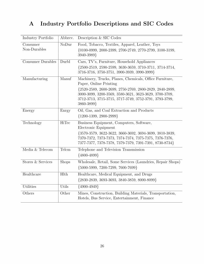
Returns reported by industry sectors are designated by Kenneth French. The ten industriesare: Consumer Non-Durables, Consumer Durables, Manufacturing, Energy, Technology, Me-dia & Telecom, Stores & Services, Utilities, and Others2. They assign each NYSE (NewYork Stock Exchange), AMEX (American Stock Exchange), and NASDAQ (NASDAQ StockMarket) stock to an industry portfolio at the end of June of year t based on its four-digitSIC (Standard Industrial Classification) code at that time. They use Compustat SIC codes3

for the fiscal year ending in calendar year t − 1. Whenever Compustat SIC codes are notavailable, they use CRSP SIC codes4 for June of year t.

Market return is compiled using the 201402 CRSP database. The T-bill return is the simpledaily rate that, over the number of trading days in the month, compounds to 1-month T-Billrate from Ibbotson and Associates, Inc. T-Bill rate is used as the risk-free rate to calculatereturn premium.

The choice of daily sampling frequency is determined based on the trade-off between addi-tional information and data source restrictions. While more information is obtained whensampling frequency is high, the additional information only has marginal and diminishingeffects on beta. That is, intraday returns are highly correlated with daily returns, meaningforgoing any more information would not significantly improve our information base. For in-stance, our data size would be seven times our current dataset if hourly returns were used butthis does not indicate that we would increase our precision of beta measurements by seventimes as well. Thus, daily returns offer a good trade-off between additional information anddata restrictions.

4.2 Data Analysis

Table 1 presents summary statistics for daily returns data for 10 US industry portfolios andmarket index covering the period from January 1960 to December 2012. All series havemean returns very close to zero. Consumer Non-Durables and Utilities have lower standarddeviation compared to others while Technology has the highest standard deviation amongall sectors. In the context of the economy, such results indicate that Technology sector tobe the most volatile in the market and Non-Durables and Utilities sectors the least volatile.In addition, minimum returns in absolute value for all sectors (including market index) arebigger than their maximum returns, indicating that all stocks are more volatile in recessionsthan booms.

2Full descriptions and SIC codes of each industry portfolio can be found in Appendix A3SIC codes provided by Standard & Poors Financial Services LLC4SIC codes provided by Center for Research in Security Prices (CRSP)

12

Table 1: Analysis of Industry Portfolio & Market Returns (1960 - 2012)

US Industry Mean Stdev. Min Max Skewness Kurtosis

Non-Durables 0.03061 0.8644 -17.06 10.28 -0.6235 22.282Durables 0.01986 1.3095 -18.38 9.72 -0.2147 11.788

Manufacturing 0.02253 1.0337 -20.03 10.74 -0.6701 21.280Energy 0.03315 1.2695 -19.46 19.33 -0.1917 19.858

Technology 0.02405 1.4266 -20.01 16.01 -0.0295 11.905Media & Telecom 0.02291 1.1026 -16.71 14.51 -0.0218 17.118Stores & Services 0.02745 1.0507 -16.60 10.99 -0.2678 13.982

Healthcare 0.02831 1.0681 -17.92 11.09 -0.4002 14.403Utilities 0.02063 0.8184 -12.89 14.43 -0.0045 29.265Others 0.02298 1.1259 -15.33 11.26 -0.2464 18.114Market 0.02180 0.9852 -17.44 11.35 -0.5203 19.235

All returns are excess returns. For simplicity and clarity of the table, all values besideskurtosis are represented in percentages (%).

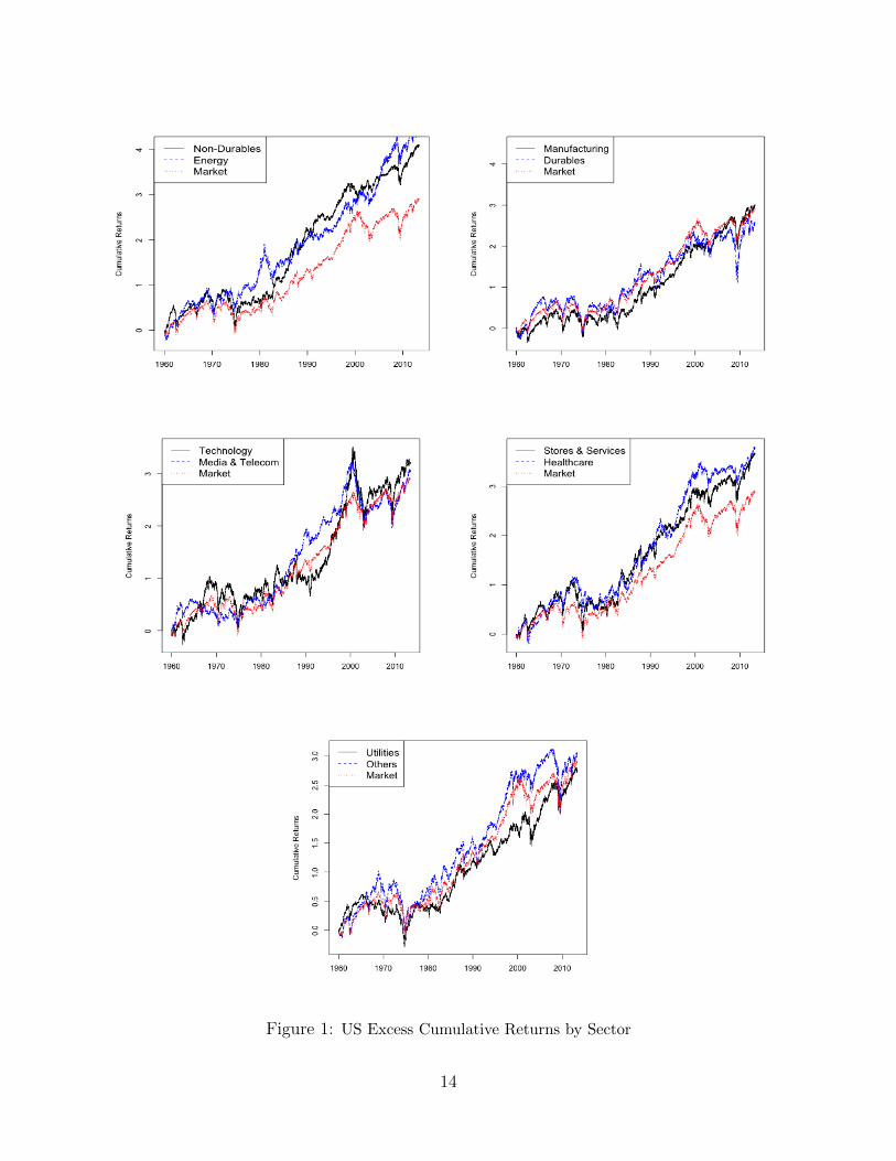
Figure 1 plots the cumulative time-series returns for industry sectors and we have seen contin-uous growth through the 1960s till present. In addition, we have observed a dip in 1973-1975(period of economic stagnation in the Western World that puts an end to post-World War IIeconomic boom), and a drop-off following the dot-com burst, followed by a slow yet steadyimprovement until the credit crisis from late 2007 and sovereign debt crisis from late 2009.In addition, All sectors and market index show a huge sudden dip in returns around October1987, which is what we generally referred to as “Black Monday” (October 19th, 1987) whenstock markets around the world crashed.

A sharp rally through early 2000 can be seen especially in the Technology and Media &Telecom sectors and a rally in Energy, Manufacturing, and Others after 2004 compared toother sectors. According to SIC Codes in Appendix A, Others include Financial Services,Entertainment, Hotels, etc. Therefore, we contribute the rally largely to booms in FinancialServices and Entertainment throughout 2003 - 2007.

13

Figure 1: US Excess Cumulative Returns by Sector

14

5 Results

For the sake of brevity, we select to report the average industry beta under different pricingand beta valuation models across the entire 52 years from 1960 to 2012 (Table 2). Then weshow the betas during contraction periods and expansion periods as defined by the NBERunder each of the asset pricing model - CAPM (Table 5) and Fama French model (Table 6).By definition, contraction periods yielded significant negative returns due to the bursting ofmany financial crises and expansion periods produced significant positive returns as economicgrowth spiked. Therefore, we select contractions as representation of bear market and andexpansions as bull market.

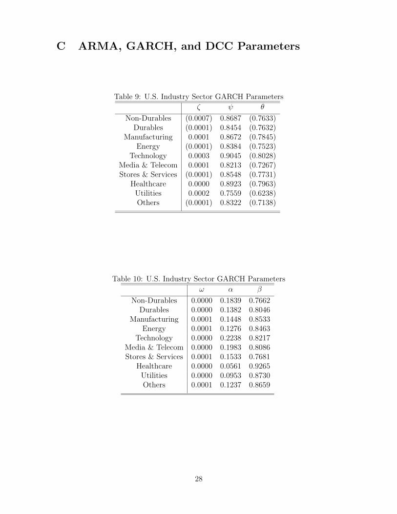
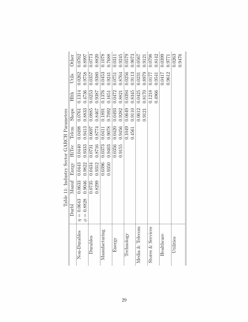
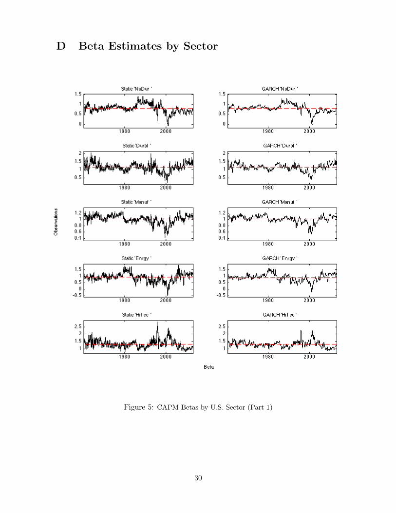
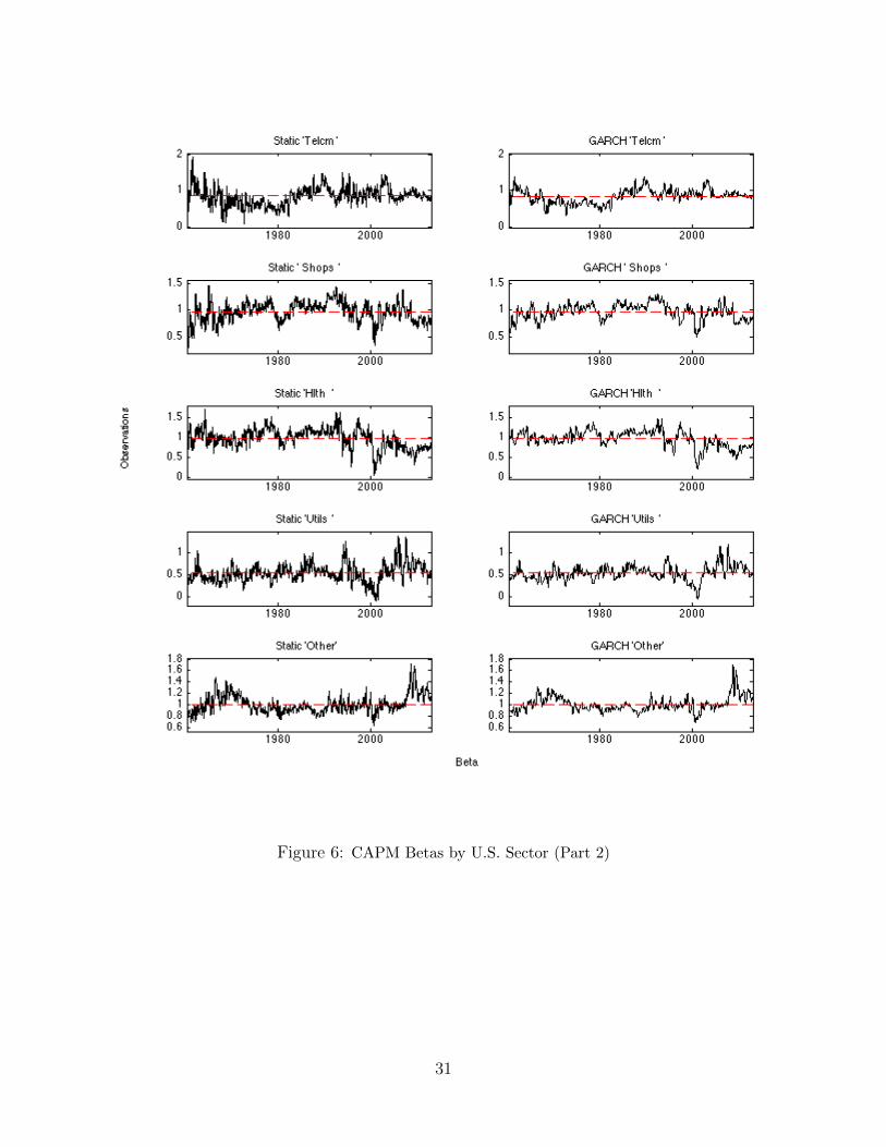
Furthermore, we select two industries, Technology and Stores & Services, to illustrate com-parison of beta estimates between models. These two industries are representative among allindustries in terms of scale and fluctation. Beta estimation comparison for all 10 industriesare shown in Appendix D. The ARMA, GARCH, and DCC parametrs for the DCC-GARCHmodel are reported in Appendix C.

5.1 Industry Average Beta Findings

Table 2 shows the average industry beta estimation using the two beta models for the CAPMand Fama-French Three Factor model5 across the entire sample period (1960 2012). Esti-mates from the two circumstances differ but not significantly. Across all sectors, Utilities hasthe lowest beta value, indicating its low exposure to market volatility as a fairly conservativeand consistent industry. Technology ranks among the most volatile sector by its nature ofbusiness and, potentially, partially due to the Internet boom and its eventual bust. Otherrelative stable industries, that is, industries with lower betas include No-Durables and Media& Telecom, while Durables demonstrates a comparatively volatile returns to the market.

Average beta estimates under similar economic environment are very similar and rather closeto 1, the market beta average. Such finding stands as mean averages out any anomalies witha short period of time across a long time-span. The GARCH beta estimates are consistentlyslightly lower than Static betas between the two beta models used. Moreover, from figuresin Appendix D, it can be found that beta curves from GARCH model are smoother and inmost cases have smaller maximum and minimum beta values than the Static model, due tothe mean reversion property and momentum effect for GARCH. More interestingly, whencomparing between the two asset pricing models using identical beta modeling, Fama-Frenchbetas are slightly higher than those of CAPM for each industry.

5Fama-French betas present in all tables below correspond to the market beta term

15

Table 2: Average Industry Betas (1960 - 2012)

U.S. IndustryCAPM Fama-French

Static DCC Static DCC

Non-Durables 0.7982 0.7966 0.8043 0.7957Durables 1.1558 1.1506 1.1789 1.1510

Manufacturing 1.0165 1.1048 1.0471 1.0143Energy 0.9133 0.9103 0.9946 0.9084

Technology 1.3296 1.3171 1.1178 1.3174Media & Telecom 0.8462 0.8438 0.9173 0.8458Stores & Services 0.9669 0.9620 0.9913 0.9625

Healthcare 0.9711 0.9636 0.8766 0.9634Utilities 0.5476 0.5407 0.7033 0.5411Others 1.0122 1.0101 1.0899 1.0098

Figure 2 and 3 illustrate daily Static and GARCH betas from 1960 to 2012 in the contextof two asset pricing models for the Technology and Stores & Services Industry. Both figuresshow similar movements in betas and draw an identical conclusion that beta movementsgenerally give indication to great changes in the economy such as economic recessions orbooms. Yet the necessary correlation between the direction of beta movement and good orbad economic changes has to be established case by case. We will discuss fluctuations ofbetas in relationship with contractions and expansion in more detail in a later section.

It is interesting to note that CAPM betas offer much clearer trend of movement than Fama-French betas. This is mainly caused by absorbing effect of the other two factors in theFama-French model, making the market beta less indicative of the general market trend.Moreover, GARCH beta estimates in general, for both CAPM and Fama French, show lessswing in beta values than Static betas. This demonstrates GARCH’s mean reversion nature,which ensures stationarity in the beta values to fluctuate within a reasonable range around 1.

16

• Case 1: Technology Industry

Figure 2: Technology Industry CAPM & Fama-French Betas (1960 - 2012)

• Case 2: Stores & Services Industry

Figure 3: Stores & Services Industry CAPM & Fama-French Betas (1960 - 2012)

17

5.2 Beta Forecast Comparison

Table 3 and 4 below summarize the results of the Diebold-Mariano (DM) test over the entiresample period and presents level of significance between two beta methods and asset pricingmodels using the DM test.

5.2.1 Static vs. DCC-GARCH Beta Comparison

Table 3 shows accuracy of beta estimation using the two methods by the same asset-pricingmodel. When comparing Static beta modeling with GARCH(1,1) model under the CAPMframework, Energy, Healthcare, and Other sectors are estimated with non-signifcant accu-racy than using GARCH(1,1) model while Non-Durables, Durables, Utilities, and Media &Telecom sector demonstrate much more precision with Static beta modeling. Other sectorreturn estimations demonstrated similar goodness-of-fit and accuracy using either method.

However, under the Fama-French framework, advantages of the GARCH(1,1) model are muchmore significant across multiple vectors, namely, Durables, Manufacturing, Technology, Me-dia & Telecom, Stores & Stores, Healthcare, and Utilities. Differences in the results can beexplained by the fact that conditional volatility and correlations respond more flexibly tochanges at multivariate level.

Table 3: DM Test: Static vs. GARCH Model Precision (1960 - 2012)

U.S. Industry CAPM Fama-French U.S. Industry CAPM Fama-French

Non-Durables 1.945* 1.448 Media & Telecom 3.112*** 3.713***Durables 3.692*** 2.767*** Stores & Services 1.026 2.482***

Manufacturing 0.684 2.667*** Healthcare -0.523 2.297***Energy -0.788 1.069 Utilities 1.892* 1.951**

Technology 3.112 3.713*** Other -0.746 0.908

where *** < 1% significance level; ** < 5% significance level; * < 1% significance level

5.2.2 CAPM vs. Fama-French Framework Comparison

Table 4 compares beta estimates vertically between the CAPM and Fama-French model un-der identical beta modeling methodology. Fama French betas prove to be better that CAPMbetas in most sectors. Our conclusion aligns with past research that argued CAPM fail todemonstrate accuracy in predicting asset of portfolio returns.. There is one exception toour conclusion - the Utilities sector. Under the Static model, the CAPM model performsmarginally better than the Fama-French model in predicting Utilities sector returns. Onepossible explaination for the result is that neither of the two asset pricing models offer goodpredictions given the low exposure of this industry to the overall market.

18

Table 4: DM Test: CAPM vs. Fama-French Model Precision (1960 - 2012)

U.S. Industry Static GARCH U.S. Industry Static GARCH

Non-Durables 1.4581 2.0516** Media & Telecom 3.7186*** 3.7373***Durables 2.0909** 3.3898*** Stores & Services 3.2912*** 3.0551***

Manufactoring 1.0407 2.3173** Healthcare 3.7795*** 2.8676***Energy 0.6791 2.0162** Utilities -0.7011 1.7468**

Technology 1.7499 2.9500*** Other 2.3595** -0.7937


5.3 Beta in Recessions and Booms

Table 5 and 6 show the industry average betas estimated in recessions and booms under theCAPM and Fama-French framework respectively. Findings in Section 5.1 still apply regard-less of the economic environment. DM test is conducted to parse the best combination ofbeta and asset pricing models in economic recessions or booms.

5.3.1 Beta Fluctuations

In general, CAPM betas in the Energy, Utilities, and Others sector tend to increase inrecessions while decrease in economic booms. All other sectors show the opposite trend.Specifically, Non-Durables, Durables, Manufacturing, Technology, Media & Telecom, Stores& Services, and Healthcare are likely to decrease in beta values during contraction periods.That is, these sectors become more resistant to market turmoil during economic downturn.Minimal change in beta is seen for the Manufacturing industry while maximum in Energysector between contractionary and expansionary eras.

Fama French betas in 6 - Non-Durables, Manufacturing, Media & Telecom, Healthcare, Util-ities, and Other - out of 10 sectors betas go up in contractions and go down in expansionswhen applying the Rolling Window beta estimation methodology. It is interesting to see con-trasting results of beta trends when applied in different pricing frameworks. The discrepancyin beta performance could be due to the estimation mechanisms (i.e. SMB and HML factors)as well as different equity behaviors for valued and growth stocks for the Fama-French model.Yet, we see consistent results for the GARCH model regardless of asset pricing models. Thisfind is consistent with our assumption that GARCH inherently carry the robustness throughincorporating conditional volatility.

19

Table 5: CAPM Average Industry Betas In Business Cycles (1960 - 2012)

U.S. IndustryRolling Window DCC-GARCH

Contraction Expansion Contraction Expansion


Manufactoring 1.0175 1.0163 1.0037 1.0169Energy 0.9932 0.8981 0.9942 0.8945



Table 6: Fama-French Average Industry Betas In Business Cycles (1960 - 2012)

U.S. IndustryRolling Window DCC-GARCH



Manufactoring 1.0445 1.0163 1.0029 1.0164Energy 0.9816 0.9970 0.9896 0.8932



20

5.3.2 Interesting Example

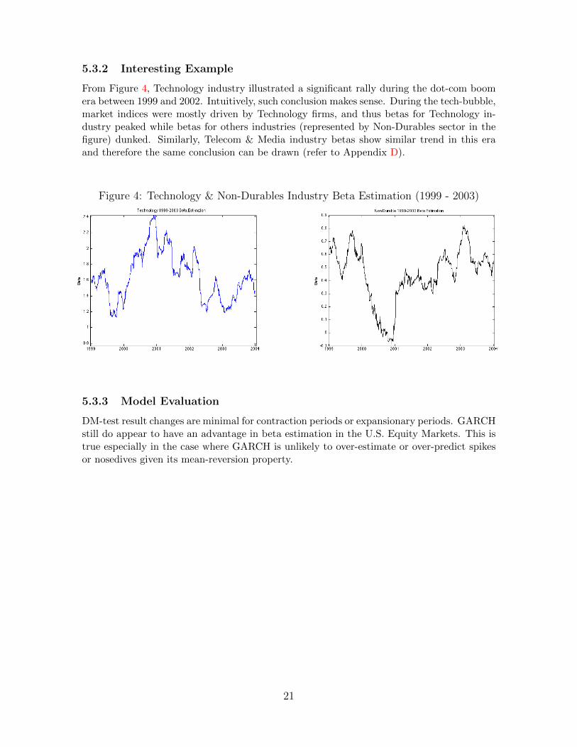
From Figure 4, Technology industry illustrated a significant rally during the dot-com boomera between 1999 and 2002. Intuitively, such conclusion makes sense. During the tech-bubble,market indices were mostly driven by Technology firms, and thus betas for Technology in-dustry peaked while betas for others industries (represented by Non-Durables sector in thefigure) dunked. Similarly, Telecom & Media industry betas show similar trend in this eraand therefore the same conclusion can be drawn (refer to Appendix D).

Figure 4: Technology & Non-Durables Industry Beta Estimation (1999 - 2003)

5.3.3 Model Evaluation

DM-test result changes are minimal for contraction periods or expansionary periods. GARCHstill do appear to have an advantage in beta estimation in the U.S. Equity Markets. This istrue especially in the case where GARCH is unlikely to over-estimate or over-predict spikesor nosedives given its mean-reversion property.

21

Table 7: DM Test: Static vs. GARCH Model Precision (Contractions & Expansions)

U.S. IndustryCAPM Fama-French


Non-Durables -1.893** -0.447 1.146 1.890*Durables 2.885*** 2.331** 1.568** 1.967**

Manufactoring -2.070*** 0.891 -0.526 1.106Energy 0.085 1.776* 2.124** 3.145***

Technology -1.579 1.629 2.089** 1.475Media & Telecom 0.866 3.228*** 3.660*** 2.249**Stores & Services 1.181 -1.658 2.939*** 1.776*

Healthcare 1.476 3.282*** 2.7158*** 3.6747***Utilities -1.579 -1.879* 1.824* 1.440Others -0.774 4.595*** 1.769* 1.839*


22

6 Conclusion

Our objective in this paper is to estimate the daily betas for industry portfolios from a rangeof variance and covariance models in an asset-pricing context using sector equity data fromthe U.S. Equity Markets. We first derive beta estimates for individual industry and theuse out-of-sample prediction for returns. We then compare our predicted returns to actualreturns to measure the effectiveness of the models in the application. Lastly, we observe thetrends and movements of the betas during U.S. economic booms and recessions.

In most cases, average beta estimates are consistent under the four methods with some excep-tions in Fama-French unconditional beta modeling. The discrepancy in model performancecould be due to the estimation mechanisms (i.e. SMB and HML factors) as well as differentequity behaviors for valued and growth stocks. On a daily basis, Static and GARCH demon-strates similar model performance under the CAPM framework; GARCH estimates result inmore accurate estimation compared to Static model using Fama-French asset pricing model.From our findings, Fama-French model do perform better than CAPM as widely perceived.We also find trends of average betas change by sectors in economic recessions or booms. Thetrends are almost consistent for the GARCH modeling while varies quite significantly for theStatic method.

In our analysis, we carry out daily estimations of 10 industry portfolios for sample period of52 years. One possible direction for future research is to extend time period back to poten-tially 1930s. This may help distinguish the underlying beta trends given more business cycles.The thesis can be further directed to compare the industry betas among large-cap, mid-cap,and small-cap stocks within each sector. Also, since U.S. Equity Markets is representative ofa financial system that is well developed, it would be also of interest to perform same exer-cise comparing beta estimates to Emerging Markets by sectors and compare how results differ.

23

Reference

[1] Andersen, T., Bollerslev, T. (1998). Answering the Skeptics: Yes. Standard VolatilityModels Do Provide Accurate Forecasts. International Economic Review, 39, 885-905.

[2] Andersen, T., Bollerslev, T., Christoffersen, P., & Diebold, F. (2006). Practical Volatilityand Correlation Modeling for Financial Market Risk Management. The Risks of FinancialInstitutions. Chicago: University of Chicago Press.

[3] Berk, J., Green, R., & Naik, V. (1999). Optimal Investment, Growth Options, andSecurity Returns. The Journal of Finance, 54, 1553-1607.

[4] Bollerslev, T. (1986). Generalized autoregressive conditional heteroskedasticity. Jour-nal of Econometrics, 31(3), 307-327

[5] Braun, P. A., Nelson, D. B., & Sunier, A. M. (1995). Good News, Bad News, Volatility,and Betas. The Journal of Finance, 50, 1575-1603.

[6] Brooks, R., Iorio, A. D., Faff, R., & Wang, Y. (2009). Testing the Integration of theUS and Chinese Stock Markets in a Fama-French Framework. Journal of Economic Integra-tion, 24, 435-454.

[7] Campbell, J. Y., Lettau, M., Malkiel, B., & Xu, Y. (2001). Have Individual StocksBecome More Volatile? An Empirical Exploration of Idiosyncratic Risk. The Journal ofFinance, 56(1), 1-43.

[8] Campbell, J. Y., & Vuolteenaho T. (2003). Bad Beta, Good Beta. Cambridge, MA:National Bureau of Economic Research.

[9] Chung, P. Y., Johnson, H., & Schill M. J. (2004). Asset Pricing When Returns areNon-Normal: Fama-French Factors vs. Higher-Order Systematic Co-Moments. Journal ofBusiness, forthcoming.

[10] Engle, R. (2002a). Dynamic Conditional Correlation: a Simple Class of MultivariateGeneralized Autoregressive Conditional Heteroskedasticity Models. The Journal of Business& Economic Statistics, 20, 339-350.

[11] Engle, R., & Patton, A. (2001). What Good is Volatility Model? Quantitative Fi-nance, 1, 237-245.

[12] Fama, E. F., MacBeth, J. D. (1973). Risk, Return, and Equilibrium: Empirical Tests.Journal of Political Economy, 81, 607-636.

[13] Fleming, J., Kirby, C., Ostdiek, B. (2003). The Econimic Value of Volatility TimingUsing Realized Volatility. Journal of Financial Economics, 67, 473-509.

[14] Ghysels, E. (1998). On Stable Factor Structures in the Pricing of Risk: Do Time-Varying Betas Help or Hurt?. Journal of Finance, 53, 549-573.

24

[15] Jostova, G., & Philipov, A. (2005). Bayesian Analysis of Stochastic Betas. The Journalof Financial and Quantitative Analysis, 40, 747-778.

[16] Lakonishok, J., Schleifer, A., & Vishny, R. W. (1994). Contrarian Investment, Ex-trapolation, and Risk. The Journal of Finance, 49, 1541-1578.

[17] Lintner J. (1965a). Security Prices, Risk, and Maximal Gains from Diversification.The Journal of Finance, 20, 587-615.

[18] Lintner J. (1965b). The Valuation of Risky Assets and the Selection of Risky Investmentsin Stock Portfolios and Capital Budgets. Review of Economics and Statistics, 47, 13-37.

[19] Mandelker, G. (1974). Risk and Return: The Case of Merging Firms. Journal ofFinancial Economics, 4, 303-335

[20] Merton, R. C. (1980). On Estimating the Expected Return on the Market: An Ex-ploratory Investigation. Journal of Financial Economics, 8, 323-361.

[21] Officer, R. (1973). The Variability of the Market Factor of the New York Stock Ex-change. Journal of Business, 46, 434-453.

[22] Ozoguz, A. (2009). Good Times or Bad Times? Investors’ Uncertainty and StockReturns. The Review of Financial Studies, 22, 4377-4422.

[23] Sharpe W. F. (1964). Capital Asset Prices A Theory of Market Equilibrium UnderConditions of Risk. The Journal of Finance, 19, 425-442

[24] Sonik, B., Boucrelle, C., & Le Fur, Y. (1996). International Market Correlation andVolatility. Financial Analysts Journal, 52(5), 17-34.

[25] Wiggins, J. (1992). Estimating the Volatility of S&P 500 Future Prices Using theExtreme-Value Method. Journal of Future Markets, 12(3), 256-273.

25

A Industry Portfolio Descriptions and SIC Codes

Industry Portfolio Abbrev. Description & SIC Codes

ConsumerNon-Durables

NoDur Food, Tobacco, Textiles, Apparel, Leather, Toys

{0100-0999, 2000-2399, 2700-2749, 2770-2799, 3100-3199,3940-3989}

Consumer Durables Durbl Cars, TV’s, Furniture, Household Appliances

{2500-2519, 2590-2599, 3630-3659, 3710-3711, 3714-3714,3716-3716, 3750-3751, 3900-3939, 3990-3999}

Manufacturing Manuf Machinery, Trucks, Planes, Chemicals, Office Furniture,Paper, Online Printing

{2520-2589, 2600-2699, 2750-2769, 2800-2829, 2840-2899,3000-3099, 3200-3569, 3580-3621, 3623-3629, 3700-3709,3712-3713, 3715-3715, 3717-3749, 3752-3791, 3793-3799,3860-3899}

Energy Enrgy Oil, Gas, and Coal Extraction and Products

{1200-1399, 2900-2999}Technology HiTec Business Equipment, Computers, Software,

Electronic Equipment

{3570-3579, 3622-3622, 3660-3692, 3694-3699, 3810-3839,7370-7372, 7373-7373, 7374-7374, 7375-7375, 7376-7376,7377-7377, 7378-7378, 7379-7379, 7391-7391, 8730-8734}

Media & Telecom Telcm Telephone and Television Transmission

{4800-4899}Stores & Services Shops Wholesale, Retail, Some Services (Laundries, Repair Shops)

{5000-5999, 7200-7299, 7600-7699}Healthcare Hlth Healthcare, Medical Equipment, and Drugs

{2830-2839, 3693-3693, 3840-3859, 8000-8099}Utilities Utils {4900-4949}Others Other Mines, Construction, Building Materials, Transportation,

Hotels, Bus Service, Entertainment, Finance

26

B NBER Business Cycle Dates

Table 8: Business Cycle Reference Dates (1960 -2012)

Peak TroughDuration in Months

Contraction Expansion

April 1960 February 1961 10 24December 1969 November 1970 11 106November 1973 March 1975 16 36January 1980 July 1980 6 58July 1981 November 1982 16 12July 1990 March 1991 8 92March 2001 November 2001 8 120December 2007 June 2009 18 73

27

C ARMA, GARCH, and DCC Parameters

Table 9: U.S. Industry Sector GARCH Parameters

ζ ψ θ

Non-Durables (0.0007) 0.8687 (0.7633)Durables (0.0001) 0.8454 (0.7632)

Manufacturing 0.0001 0.8672 (0.7845)Energy (0.0001) 0.8384 (0.7523)

Technology 0.0003 0.9045 (0.8028)Media & Telecom 0.0001 0.8213 (0.7267)Stores & Services (0.0001) 0.8548 (0.7731)

Healthcare 0.0000 0.8923 (0.7963)Utilities 0.0002 0.7559 (0.6238)Others (0.0001) 0.8322 (0.7138)

Table 10: U.S. Industry Sector GARCH Parameters

ω α β

Non-Durables 0.0000 0.1839 0.7662Durables 0.0000 0.1382 0.8046

Manufacturing 0.0001 0.1448 0.8533Energy 0.0001 0.1276 0.8463

Technology 0.0000 0.2238 0.8217Media & Telecom 0.0000 0.1983 0.8086Stores & Services 0.0001 0.1533 0.7681

Healthcare 0.0000 0.0561 0.9265Utilities 0.0000 0.0953 0.8730Others 0.0001 0.1237 0.8659

28

Tab

le11

:In

dust

rySec

tor

GA

RC

HP

aram

eter

s

Durb

lM

anuf

Enrg

yH

iTec

Tel

cmShop

sH

lth

Uti

lsO

ther

Non

-Dura

ble

sη

=0.

0643

0.06

330.

0443

0.04

400.

0498

0.07

610.

1314

0.02

620.

0762

φ=

0.88

280.

9046

0.98

220.

9333

0.94

130.

8833

0.47

360.

9758

0.89

97D

ura

ble

s0.

0735

0.04

340.

0731

0.06

970.

0885

0.02

530.

0357

0.07

730.

8299

0.93

120.

8716

0.87

740.

8467

0.93

870.

9380

0.88

20M

anufa

cturi

ng

0.03

960.

0373

0.04

110.

1891

0.13

760.

0453

0.10

780.

9350

0.94

030.

9078

0.70

920.

1651

0.92

410.

7688

Ener

gy0.

0356

0.04

200.

0493

0.04

720.

0751

0.03

110.

9155

0.94

560.

9282

0.88

210.

8764

0.92

45T

echnol

ogy

0.10

490.

0649

0.03

940.

0256

0.05

790.

4561

0.91

100.

8345

0.91

130.

9073

Med

ia&

Tel

ecom

0.06

120.

0425

0.02

310.

0567

0.91

210.

8170

0.89

790.

9121

Sto

res

&Ser

vic

es0.

1218

0.01

770.

0798

0.49

660.

9541

0.81

42H

ealt

hca

re0.

0417

0.03

990.

9612

0.97

71U

tiliti

es0.

0263

0.94

76

29

D Beta Estimates by Sector

Figure 5: CAPM Betas by U.S. Sector (Part 1)

30

Figure 6: CAPM Betas by U.S. Sector (Part 2)

31

Figure 7: Fama French Betas by U.S. Sector (Part 1)

32

Figure 8: Fama French Betas by U.S. Sector (Part 2)

33

Figure 9: Static (Rolling Window) Model Betas by U.S. Sector (Part 1)

34

Figure 10: Static (Rolling Window) Model Betas by U.S. Sector (Part 2)

35

Figure 11: DCC-GARCH Model Betas by U.S. Sector (Part 1)

36

Figure 12: DCC-GARCH Betas by U.S. Sector (Part 2)

37

Date post:	30-Apr-2018
Category:	Documents
Upload:	ngothien
View:	219 times
Download:	0 times

Conditional Beta Models for Asset Pricing by Sector in...

Documents