Topic 6 Conditional Probability and Independence One of the most important concepts in the theory of probability is based on the question: How do we modify the probability of an event in light of the fact that something new is known? What is the chance that we will win the game now that we have taken the first point? What is the chance that I am a carrier of a genetic disease now that my first child does not have the genetic condition? What is the chance that a child smokes if the household has two parents who smoke? This question leads us to the concept of conditional probability. 6.1 Restricting the Sample Space - Conditional Probability Toss a fair coin 3 times. Let winning be “at least two heads out of three” HHH HHT HTH HTT THH THT TTH TTT Figure 6.1: Outcomes on three tosses of a coin, with the winning event indicated. 0 0.2 0.4 0.6 0.8 1 1 8 6 4 2 0 2 4 6 8 1 A A B B Figure 6.2: Two Venn diagrams to illustrate conditional probability. For the top diagram P (A) is large but P (A|B) is small. For the bot- tom diagram P (A) is small but P (A|B) is large. If we now know that the first coin toss is heads, then only the top row is possible and we would like to say that the probability of winning is #(outcomes that result in a win and also have a heads on the first coin toss) #(outcomes with heads on the first coin toss) = #{HHH, HHT, HTH} #{HHH, HHT, HTH, HTT} = 3 4 . We can take this idea to create a formula in the case of equally likely outcomes for the statement the conditional probability of A given B. P (A|B)= the proportion of outcomes in A that are also in B = #(A \ B) #(B) We can turn this into a more general statement using only the probability, P , by dividing both the numerator and the denominator in this fraction by #(⌦). P (A|B)= #(A \ B)/#(⌦) #(B)/#(⌦) = P (A \ B) P (B) (6.1) We thus take this version (6.1) of the identity as the general definition of conditional probability for any pair of events A and B as long as the denominator P (B) > 0. 89
Transcript
Topic 6
Conditional Probability and Independence
One of the most important concepts in the theory of probability is based on the question: How do we modify theprobability of an event in light of the fact that something new is known? What is the chance that we will win the gamenow that we have taken the first point? What is the chance that I am a carrier of a genetic disease now that my firstchild does not have the genetic condition? What is the chance that a child smokes if the household has two parentswho smoke? This question leads us to the concept of conditional probability.
6.1 Restricting the Sample Space - Conditional ProbabilityToss a fair coin 3 times. Let winning be “at least two heads out of three”
HHH HHT HTH HTTTHH THT TTH TTT
Figure 6.1: Outcomes on three tosses of a coin, with the winning event indicated.
0 0.2 0.4 0.6 0.8 1−1
−0.8
−0.6
−0.4
−0.2
0
0.2
0.4
0.6
0.8
1
A
A
B
B
Figure 6.2: Two Venn diagramsto illustrate conditional probability.For the top diagram P (A) is largebut P (A|B) is small. For the bot-tom diagram P (A) is small butP (A|B) is large.
If we now know that the first coin toss is heads, then only the top row is possibleand we would like to say that the probability of winning is
#(outcomes that result in a win and also have a heads on the first coin toss)#(outcomes with heads on the first coin toss)
=
#{HHH, HHT, HTH}#{HHH, HHT, HTH, HTT} =
3
4
.
We can take this idea to create a formula in the case of equally likely outcomes forthe statement the conditional probability of A given B.
P (A|B) = the proportion of outcomes in A that are also in B
=
#(A \B)
#(B)
We can turn this into a more general statement using only the probability, P , bydividing both the numerator and the denominator in this fraction by #(⌦).
P (A|B) =
#(A \B)/#(⌦)
#(B)/#(⌦)
=
P (A \B)
P (B)
(6.1)
We thus take this version (6.1) of the identity as the general definition of conditionalprobability for any pair of events A and B as long as the denominator P (B) > 0.
89
Introduction to the Science of Statistics Conditional Probability and Independence
Exercise 6.1. Pick an event B so that P (B) > 0. Define, for every event A,
Q(A) = P (A|B).
Show that Q satisfies the three axioms of a probability. In words, a conditional probability is a probability.
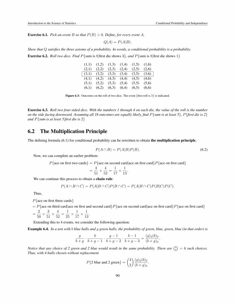
Exercise 6.2. Roll two dice. Find P{sum is 8|first die shows 3}, and P{sum is 8|first die shows 1}
Figure 6.3: Outcomes on the roll of two dice. The event {first roll is 3} is indicated.
Exercise 6.3. Roll two four-sided dice. With the numbers 1 through 4 on each die, the value of the roll is the numberon the side facing downward. Assuming all 16 outcomes are equally likely, find P{sum is at least 5}, P{first die is 2}and P{sum is at least 5|first die is 2}
6.2 The Multiplication PrincipleThe defining formula (6.1) for conditional probability can be rewritten to obtain the multiplication principle,
P (A \B) = P (A|B)P (B). (6.2)
Now, we can complete an earlier problem:
P{ace on first two cards} = P{ace on second card|ace on first card}P{ace on first card}
=
3
51
⇥ 4
52
=
1
17
⇥ 1
13
.
We can continue this process to obtain a chain rule:
P (A \B \ C) = P (A|B \ C)P (B \ C) = P (A|B \ C)P (B|C)P (C).
Thus,
P{ace on first three cards}= P{ace on third card|ace on first and second card}P{ace on second card|ace on first card}P{ace on first card}
=
2
50
⇥ 3
51
⇥ 4
52
=
1
25
⇥ 1
17
⇥ 1
13
.
Extending this to 4 events, we consider the following question:
Example 6.4. In a urn with b blue balls and g green balls, the probability of green, blue, green, blue (in that order) is
g
b+ g· b
b+ g � 1
· g � 1
b+ g � 2
· b� 1
b+ g � 3
=
(g)2
(b)2
(b+ g)4
.
Notice that any choice of 2 green and 2 blue would result in the same probability. There are�
4
2
�
= 6 such choices.Thus, with 4 balls chosen without replacement
P{2 blue and 2 green} =
✓
4
2
◆
(g)2
(b)2
(b+ g)4
.
90
Introduction to the Science of Statistics Conditional Probability and Independence
Exercise 6.5. Show that✓
4
2
◆
(g)2
(b)2
(b+ g)4
=
�b2
��g2
�
�b+g4
� .
Explain in words why P{2 blue and 2 green} is the expression on the right.
We will later extend this idea when we introduce sampling without replacement in the context of the hypergeomet-ric random variable.
6.3 The Law of Total ProbabilityIf we know the fraction of the population in a given state of the United States that has a given attribute - is diabetic,over 65 years of age, has an income of $100,000, owns their own home, is married - then how do we determine whatfraction of the total population of the United States has this attribute? We address this question by introducing aconcept - partitions - and an identity - the law of total probability.
Definition 6.6. A partition of the sample space ⌦ is a finite collection of pairwise mutually exclusive events
{C1
, C2
, . . . , Cn}
whose union is ⌦.
−0.2 0 0.2 0.4 0.6 0.8 1 1.2−0.2
0
0.2
0.4
0.6
0.8
1
1.2
C1
C2
C3
C5
C4 C
6
C7
C8
C9
A
Figure 6.4: A partition {C1 . . . , C9} of the sample space ⌦. The event A can bewritten as the union (A \ C1) [ · · · [ (A \ C9) of mutually exclusive events.
Thus, every outcome ! 2 ⌦ belongs to ex-actly one of the Ci. In particular, distinct mem-bers of the partition are mutually exclusive. (Ci\Cj = ;, if i 6= j)
If we know the fraction of the population from18 to 25 that has been infected by the H1N1 in-fluenza A virus in each of the 50 states, then wecannot just average these 50 values to obtain thefraction of this population infected in the wholecountry. This method fails because it give equalweight to California and Wyoming. The law oftotal probability shows that we should weighthese conditional probabilities by the probabilityof residence in a given state and then sum over allof the states.
Theorem 6.7 (law of total probability). Let P bea probability on ⌦ and let {C
1
, C2
, . . . , Cn} be apartition of ⌦ chosen so that P (Ci) > 0 for all i.Then, for any event A ⇢ ⌦,
P (A) =
nX
i=1
P (A|Ci)P (Ci). (6.3)
Because {C1
, C2
, . . . , Cn} is a partition, {A \ C1
, A \ C2
, . . . , A \ Cn} are pairwise mutually exclusive events.By the distributive property of sets, their union is the event A. (See Figure 6.4.)
To refer the example above the Ci are the residents of state i, A \ Ci are those residents who are from 18 to 25years old and have been been infected by the H1N1 influenza A virus. Thus, distinct A \ Ci are mutually exclusive -individuals cannot reside in 2 different states. Their union is A, all individuals in the United States between the agesof 18 and 25 years old who have been been infected by the H1N1 virus.
91
Introduction to the Science of Statistics Conditional Probability and Independence
A
CcC
Figure 6.5: A partition into two events C and Cc.
Thus,
P (A) =
nX
i=1
P (A \ Ci). (6.4)
Finish by using the multiplication identity (6.2),
P (A \ Ci) = P (A|Ci)P (Ci), i = 1, 2, . . . , n
and substituting into (6.4) to obtain the identity in (6.3).The most frequent use of the law of total probability
comes in the case of a partition of the sample space intotwo events, {C,Cc}. In this case the law of total probabilitybecomes the identity
P (A) = P (A|C)P (C) + P (A|Cc)P (Cc
). (6.5)
Exercise 6.8. The problem of points is a classical problemin probability theory. The problem concerns a series of games with two sides who have equal chances of winning eachgame. The winning side is one that first reaches a given number n of wins. Let n = 4 for a best of seven playoff.Determine
pij = P{winning the playoff after i wins vs j opponent wins}
(Hint: pii = 1
2
for i = 0, 1, 2, 3.)
6.4 Bayes formulaLet A be the event that an individual tests positive for some disease and C be the event that the person actually hasthe disease. We can perform clinical trials to estimate the probability that a randomly chosen individual tests positivegiven that they have the disease,
P{tests positive|has the disease} = P (A|C),
by taking individuals with the disease and applying the test. However, we would like to use the test as a method ofdiagnosis of the disease. Thus, we would like to be able to give the test and assert the chance that the person has thedisease. That is, we want to know the probability with the reverse conditioning
P{has the disease|tests positive} = P (C|A).
Example 6.9. The Public Health Department gives us the following information.
• A test for the disease yields a positive result 90% of the time when the disease is present.
• A test for the disease yields a positive result 1% of the time when the disease is not present.
• One person in 1,000 has the disease.
Let’s first think about this intuitively and then look to a more formal way using Bayes formula to find the probabilityof
P (C|A).
• In a city with a population of 1 million people, on average,
1,000 have the disease and 999,000 do not
• Of the 1,000 that have the disease, on average,
92
Introduction to the Science of Statistics Conditional Probability and Independence
1,000,000 people�����
AAAAU
1,000 have the disease
999,000 do not have the disease���
AAU
���
AAU
900 test positive
100 test negative
9,990 test positive
989,010 test negative
P (C) = 0.001
P (Cc) = 0.999
P (A|C)P (C) = 0.0009
P (Ac|C)P (C) = 0.0001
P (A|Cc)P (Cc) = 0.00999
P (Ac|Cc)P (Cc) = 0.98901
Figure 6.6: Tree diagram. We can use a tree diagram to indicate the number of individuals, on average, in each group (in black) or the probablity(in blue). Notice that in each column the number of individuals adds to give 1,000,000 and the probabilities add to give 1. In addition, each pair ofarrows divides an events into two mutually exclusive subevents. Thus, both the numbers and the probabilities at the tip of the arrows add to give therespective values at the head of the arrow.
900 test positive and 100 test negative
• Of the 999,000 that do not have the disease, on average,
999,000 ⇥ 0.01 = 9990 test positive and 989,010 test negative.
Consequently, among those that test positive, the odds of having the disease is
#(have the disease):#(does not have the disease)
900:9990
and converting odds to probability we see that
P{have the disease|test is positive} =
900
900 + 9990
= 0.0826.
We now derive Bayes formula. First notice that we can flip the order of conditioning by using the multiplicationformula (6.2) twice
P (A \ C) =
8
<
:
P (A|C)P (C)
P (C|A)P (A)
Now we can create a formula for P (C|A) as desired in terms of P (A|C).
P (C|A)P (A) = P (A|C)P (C) or P (C|A) =
P (A|C)P (C)
P (A)
.
Thus, given A, the probability of C changes by the Bayes factorP (A|C)
P (A)
.
93
Introduction to the Science of Statistics Conditional Probability and Independence
public healthresearcher worker clinician
has does not has does notdisease have disease �! disease have disease
C Cc C Cc sumtests positive P (A|C) P (A|Cc
) P (C) = 0.001 tests positive P (C|A) P (Cc|A)
A 0.90 0.01 P (Cc) = 0.999 A 0.0826 0.9174 1
tests negative P (Ac|C) P (Ac|Cc) tests negative P (C|Ac
) P (Cc|Ac)
Ac 0.10 0.99 - Ac 0.0001 0.9999 1sum 1 1
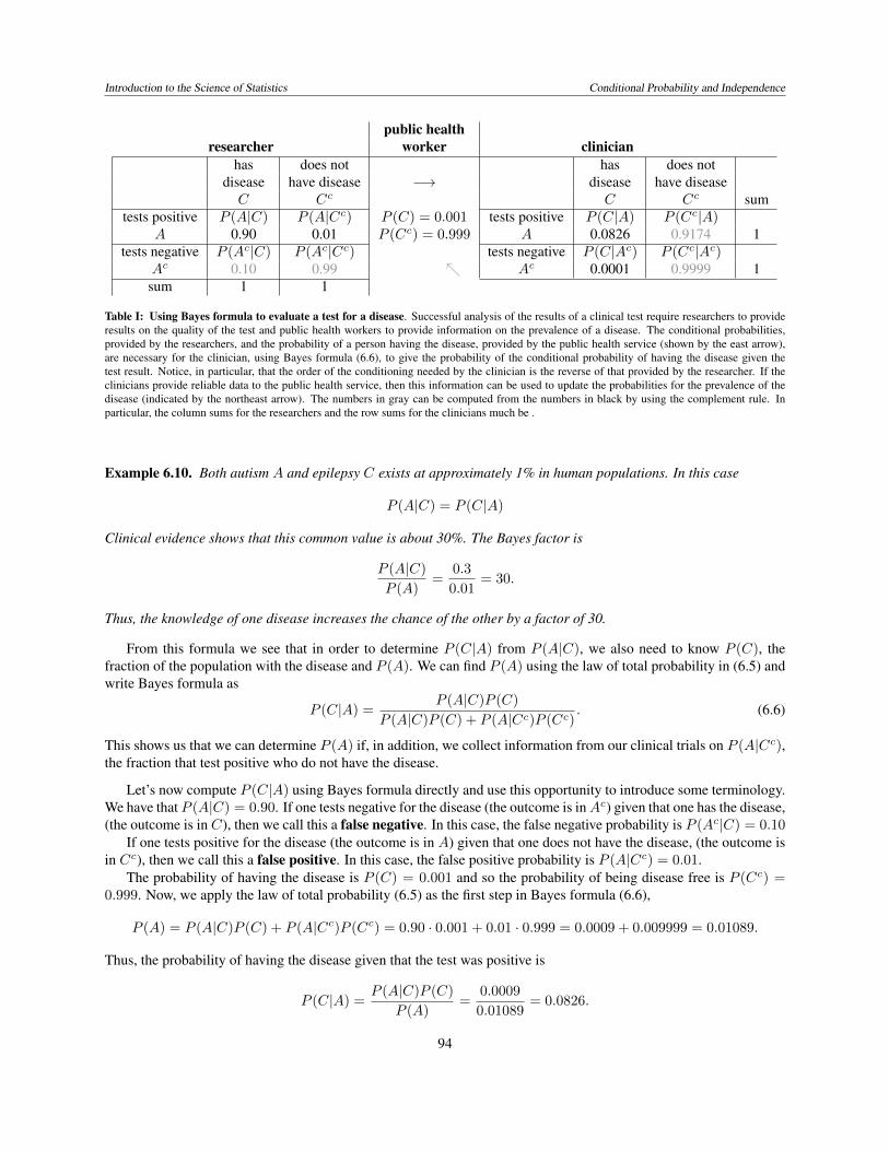
Table I: Using Bayes formula to evaluate a test for a disease. Successful analysis of the results of a clinical test require researchers to provideresults on the quality of the test and public health workers to provide information on the prevalence of a disease. The conditional probabilities,provided by the researchers, and the probability of a person having the disease, provided by the public health service (shown by the east arrow),are necessary for the clinician, using Bayes formula (6.6), to give the probability of the conditional probability of having the disease given thetest result. Notice, in particular, that the order of the conditioning needed by the clinician is the reverse of that provided by the researcher. If theclinicians provide reliable data to the public health service, then this information can be used to update the probabilities for the prevalence of thedisease (indicated by the northeast arrow). The numbers in gray can be computed from the numbers in black by using the complement rule. Inparticular, the column sums for the researchers and the row sums for the clinicians much be .
Example 6.10. Both autism A and epilepsy C exists at approximately 1% in human populations. In this case
P (A|C) = P (C|A)
Clinical evidence shows that this common value is about 30%. The Bayes factor is
P (A|C)
P (A)
=
0.3
0.01= 30.
Thus, the knowledge of one disease increases the chance of the other by a factor of 30.
From this formula we see that in order to determine P (C|A) from P (A|C), we also need to know P (C), thefraction of the population with the disease and P (A). We can find P (A) using the law of total probability in (6.5) andwrite Bayes formula as
P (C|A) =
P (A|C)P (C)
P (A|C)P (C) + P (A|Cc)P (Cc
)
. (6.6)
This shows us that we can determine P (A) if, in addition, we collect information from our clinical trials on P (A|Cc),
the fraction that test positive who do not have the disease.
Let’s now compute P (C|A) using Bayes formula directly and use this opportunity to introduce some terminology.We have that P (A|C) = 0.90. If one tests negative for the disease (the outcome is in Ac) given that one has the disease,(the outcome is in C), then we call this a false negative. In this case, the false negative probability is P (Ac|C) = 0.10
If one tests positive for the disease (the outcome is in A) given that one does not have the disease, (the outcome isin Cc), then we call this a false positive. In this case, the false positive probability is P (A|Cc
) = 0.01.The probability of having the disease is P (C) = 0.001 and so the probability of being disease free is P (Cc
) =
0.999. Now, we apply the law of total probability (6.5) as the first step in Bayes formula (6.6),
Thus, the probability of having the disease given that the test was positive is
P (C|A) =
P (A|C)P (C)
P (A)
=
0.0009
0.01089= 0.0826.
94
Introduction to the Science of Statistics Conditional Probability and Independence
Notice that the numerator is one of the terms that was summed to compute the denominator.The answer in the previous example may be surprising. Only 8% of those who test positive actually have the
disease. This example underscores the fact that good predictions based on intuition are hard to make in this case. Todetermine the probability, we must weigh the odds of two terms, each of them itself a product.
• P (A|C)P (C), a big number (the true positive probability) times a small number (the probability of having thedisease) versus
• P (A|Cc)P (Cc
), a small number (the false positive probability) times a large number (the probability of beingdisease free).
We do not need to restrict Bayes formula to the case of C, has the disease, and Cc, does not have the disease, asseen in (6.5), but rather to any partition of the sample space. Indeed, Bayes formula can be generalized to the case ofa partition {C
1
, C2
, . . . , Cn} of ⌦ chosen so that P (Ci) > 0 for all i. Then, for any event A ⇢ ⌦ and any j
P (Cj |A) =
P (A|Cj)P (Cj)Pn
i=1
P (A|Ci)P (Ci). (6.7)
To understand why this is true, use the law of total probability to see that the denominator is equal to P (A). Bythe multiplication identity for conditional probability, the numerator is equal to P (Cj \ A). Now, make these twosubstitutions into (6.7) and use one more time the definition of conditional probability.
Example 6.11. We begin with a simple and seemingly silly example involving fair and two sided coins. However, weshall soon see that this leads us to a question in the vertical transmission of a genetic disease.
A box has a two-headed coin and a fair coin. It is flipped n times, yielding heads each time. What is the probabilitythat the two-headed coin is chosen?
Notice that as n increases, the probability of a two headed coin approaches 1 - with a longer and longer sequenceof heads we become increasingly suspicious (but, because the probability remains less than one, are never completelycertain) that we have chosen the two headed coin.
This is the related genetics question: Based on the pedigree of her past, a female knows that she has in her historya allele on her X chromosome that indicates a genetic condition. The allele for the condition is recessive. Becauseshe does not have the condition, she knows that she cannot be homozygous for the recessive allele. Consequently, shewants to know her chance of being a carrier (heteorzygous for a recessive allele) or not a carrier (homozygous for thecommon genetic type) of the condition. The female is a mother with n male offspring, none of which show the recessiveallele on their single X chromosome and so do not have the condition. What is the probability that the female is not acarrier?
95
Introduction to the Science of Statistics Conditional Probability and Independence
Let’s look at the computation above again, based on her pedigree, the female estimates that
P{mother is not a carrier} = p, P{mother is a carrier} = 1� p.
Then, from the law of total probability
P{n male offspring condition free}= P{n male offspring condition free|mother is not a carrier}P{mother is not a carrier}
+P{n male offspring condition free|mother is a carrier}P{mother is a carrier}= 1 · p+ 2
�n · (1� p).
and Bayes formula
P{mother is not a carrier|n male offspring condition free}
=
P{n male offspring condition free|mother is not a carrier}P{mother is not a carrier}P{n male offspring condition free}
=
1 · p1 · p+ 2
�n · (1� p)=
p
p+ 2
�n(1� p)
=
2
np
2
np+ (1� p).
Again, with more sons who do not have the condition, we become increasingly more certain that the mother is nota carrier.
One way to introduce Bayesian statistics is to consider the situation in which we do not know the value of p andreplace it with a probability distribution. Even though we will concentrate on classical approaches to statistics, wewill take the time in later sections to explore the Bayesian approach
Figure 6.7: The Venn diagram for independent events is repre-sented by the horizontal strip A and the vertical strip B is shownabove. The identity P (A \ B) = P (A)P (B) is now representedas the area of the rectangle. Other aspects of Exercise 6.12 areindicated in this Figure.
An event A is independent of B if its Bayes factor is 1, i.e.,
1 =
P (A|B)
P (A)
, P (A) = P (A|B).
In words, the occurrence of the event B does not alter theprobability of the event A. Multiply this equation by P (B)
and use the multiplication rule to obtain
P (A)P (B) = P (A|B)P (B) = P (A \B).
The formula
P (A)P (B) = P (A \B) (6.8)
is the usual definition of independence and is symmetric in theevents A and B. If A is independent of B, then B is indepen-dent of A. Consequently, when equation (6.8) is satisfied, wesay that A and B are independent.
Example 6.12. Roll two dice.
1
36
= P{a on the first die, b on the second die}
=
1
6
⇥ 1
6
= P{a on the first die}P{b on the second die}
and, thus, the outcomes on two rolls of the dice are independent.
96
Introduction to the Science of Statistics Conditional Probability and Independence
Exercise 6.13. If A and B are independent, then show that Ac and B, A and Bc, Ac and Bc are also independent.
We can also use this to extend the definition to n independent events:
Definition 6.14. The events A1
, · · · , An are called independent if for any choice Ai1 , Ai2 , · · · , Aik
taken from thiscollection of n events, then
P (Ai1 \Ai2 \ · · · \Aik
) = P (Ai1)P (Ai2) · · ·P (Aik
). (6.9)
A similar product formula holds if some of the events are replaced by their complement.
Exercise 6.15. Flip 10 biased coins. Their outcomes are independent with the i-th coin turning up heads with proba-bility pi. Find
Example 6.16. Mendel studied inheritance by conducting experiments using a garden peas. Mendel’s First Law, thelaw of segregation states that every diploid individual possesses a pair of alleles for any particular trait and that eachparent passes one randomly selected allele to its offspring.
In Mendel’s experiment, each of the 7 traits under study express themselves independently. This is an example ofMendel’s Second Law, also known as the law of independent assortment. If the dominant allele was present in thepopulation with probability p, then the recessive allele is expressed in an individual when it receive this allele fromboth of its parents. If we assume that the presence of the allele is independent for the two parents, then
This number can also be computed by added the three alternatives shown in the Punnett square in Table 6.1.
p2 + 2p(1� p) = p2 + 2p� 2p2 = 2p� p2.
Next, we look at two traits - 1 and 2 - with the dominant alleles present in the population with probabilities p1
andp2
. If these traits are expressed independently, then, we have, for example, that
P{dominant allele expressed in trait 1, recessive trait expressed in trait 2}= P{dominant allele expressed in trait 1}⇥ P{recessive trait expressed in trait 2}= (1� (1� p
1
)
2
)(1� p2
)
2.
Exercise 6.17. Show that if two traits are genetically linked, then the appearance of one increases the probability ofthe other. Thus,
P{individual has allele for trait 1|individual has allele for trait 2} > P{individual has allele for trait 1}.
implies
P{individual has allele for trait 2|individual has allele for trait 1} > P{individual has allele for trait 2}.
More generally, for events A and B,
P (A|B) > P (A) implies P (B|A) > P (B) (6.10)
then we way that A and B are positively associated.
97
Introduction to the Science of Statistics Conditional Probability and Independence
Exercise 6.18. A genetic marker B for a disease A is one in which P (A|B) ⇡ 1. In this case, approximate P (B|A).
Definition 6.19. Linkage disequilibrium is the non-independent association of alleles at two loci on single chromo-some. To define linkage disequilibrium, let
• A be the event that a given allele is present at the first locus, and
• B be the event that a given allele is present at a second locus.
Then the linkage disequilibrium,DA,B = P (A)P (B)� P (A \B).
Thus if DA,B = 0, the the two events are independent.
Exercise 6.20. Show that DA,Bc
= �DA,B
6.6 Answers to Selected Exercises S s
S SS Ssp2 p(1� p)
s sS ss(1� p)p (1� p)2
Table II: Punnett square for a monohybrid cross using a dominanttrait S (say spherical seeds) that occurs in the population with proba-bility p and a recessive trait s (wrinkled seeds) that occurs with proba-bility 1� p. Maternal genotypes are listed on top, paternal genotypeson the left. See Example 6.14. The probabilities of a given genotypeare given in the lower right hand corner of the box.
6.1. Let’s check the three axioms;
1. For any event A,
Q(A) = P (A|B) =
P (A \B)
P (B)
� 0.
2. For the sample space ⌦,
Q(⌦) = P (⌦|B) =
P (⌦ \B)
P (B)
=
P (B)
P (B)
= 1.
3. For mutually exclusive events, {Aj ; j � 1}, we havethat {Aj \B; j � 1} are also mutually exclusive and
Q
0
@
1[
j=1
Aj
1
A
= P
0
@
1[
j=1
Aj
�
�
�
B
1
A
=
P⇣⇣
S1j=1
Aj
⌘
\B⌘
P (B)
=
P (
S1j=1
(Aj \B))
P (B)
=
P1j=1
P (Aj \B)
P (B)
=
1X
j=1
P (Aj \B)
P (B)
=
1X
j=1
P (Aj |B) =
1X
j=1
Q(Aj)
6.2. P{sum is 8|first die shows 3} = 1/6, and P{sum is 8|first die shows 1} = 0.
1 2 3 41 ⇥2 ⇥ ⇥3 ⇥ ⇥ ⇥4 ⇥ ⇥ ⇥ ⇥
6.3 Here is a table of outcomes. The symbol ⇥ indicates an outcome in the event{sum is at least 5}. The rectangle indicates the event {first die is 2}. Becausethere are 10 ⇥’s,
P{sum is at least 5} = 10/16 = 5/8.
The rectangle contains 4 outcomes, so
P{first die is 2} = 4/16 = 1/4.
Inside the event {first die is 2}, 2 of the outcomes are also in the event {sum is at least 5}. Thus,
P{sum is at least 5}|first die is 2} = 2/4 = 1/2
98
Introduction to the Science of Statistics Conditional Probability and Independence
Using the definition of conditional probability, we also have
P{sum is at least 5}|first die is 2} =
P{sum is at least 5 and first die is 2}P{first die is 2} =
2/16
4/16=
2
4
=
1
2
.
6.5. We modify both sides of the equation.✓
4
2
◆
(g)2
(b)2
(b+ g)4
=
4!
2!2!
(g)2
(b)2
(b+ g)4
�b2
��g2
�
�b+g4
� =
(b)2
/2! · (g)2
/2!
(b+ g)4
/4!=
4!
2!2!
(g)2
(b)2
(b+ g)4
.
The sample space ⌦ is set of collections of 4 balls out of b+ g. This has�b+g
4
�
outcomes. The number of choices of 2blue out of b is
�b2
�
. The number of choices of 2 green out of g is�g2
�
. Thus, by the fundamental principle of counting,the total number of ways to obtain the event 2 blue and 2 green is
�b2
��g2
�
. For equally likely outcomes, the probabilityis the ratio of
�b2
��g2
�
, the number of outcomes in the event, and�b+g
4
�
, the number of outcomes in the sample space.
6.8. Let Aij be the event of winning the series that has i wins versus j wins for the opponent. Then pij = P (Aij). Weknow that
p0,4 = p
1,4 = p2,4 = p
3,4 = 0
because the series is lost when the opponent has won 4 games. Also,
p4,0 = p
4,1 = p4,2 = p
4,3 = 1
because the series is won with 4 wins in games. For a tied series, the probability of winning the series is 1/2 for bothsides.
p0,0 = p
1,1 = p2,2 = p
3,3 =
1
2
.
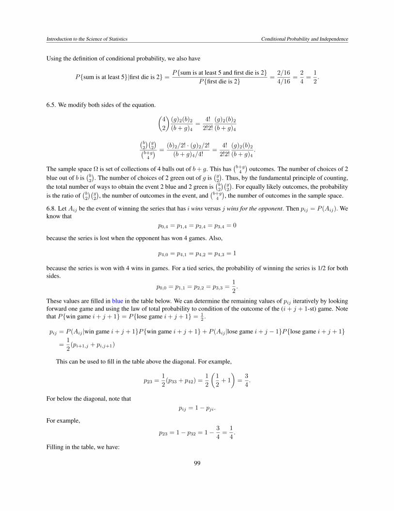
These values are filled in blue in the table below. We can determine the remaining values of pij iteratively by lookingforward one game and using the law of total probability to condition of the outcome of the (i+ j + 1-st) game. Notethat P{win game i+ j + 1} = P{lose game i+ j + 1} =
1
2
.
pij = P (Aij |win game i+ j + 1}P{win game i+ j + 1}+ P (Aij |lose game i+ j � 1}P{lose game i+ j + 1}
=
1
2
(pi+1,j + pi,j+1
)
This can be used to fill in the table above the diagonal. For example,
p23
=
1
2
(p33
+ p42
) =
1
2
✓
1
2
+ 1
◆
=
3
4
.
For below the diagonal, note thatpij = 1� pji.
For example,
p23
= 1� p32
= 1� 3
4
=
1
4
.
Filling in the table, we have:
99
Introduction to the Science of Statistics Conditional Probability and Independence