Conditional Risk Minimizationfor Stochastic Processes

Alexander ZiminIST Austria

3400 Klosterneuburg, Austriaazimin@ist.ac.at

Christoph H. LampertIST Austria

3400 Klosterneuburg, Austriachl@ist.ac.at

Abstract

We study the task of learning from non-i.i.d. data. In particular, we aim at learn-ing predictors that minimize the conditional risk for a stochastic process, i.e. theexpected loss of the predictor on the next point conditioned on the set of trainingsamples observed so far. For non-i.i.d. data, the training set contains informationabout the upcoming samples, so learning with respect to the conditional distribu-tion can be expected to yield better predictors than one obtains from the classicalsetting of minimizing the marginal risk. Our main contribution is a practical es-timator for the conditional risk based on the theory of non-parametric time-seriesprediction, and a finite sample concentration bound that establishes uniform con-vergence of the estimator to the true conditional risk under certain regularity as-sumptions on the process.

1 Introduction

One of the cornerstone assumptions in the analysis of machine learning algorithms is that the train-ing examples are independently and identically distributed (i.i.d.). Interestingly, this assumption ishardly ever fulfilled in practice: dependencies between examples exist even in the famous textbookexample of classifying e-mails into ham or spam. For example, when multiple emails are exchangedwith the same writer, the contents of later emails depends on the contents of earlier ones. For thisreason, there is growing interest in the development of algorithms that learn from dependent dataand still offer generalization guarantees similar to the i.i.d. situation.

In this work, we are interested in learning algorithms for stochastic processes, i.e. data sources withsamples arriving in a sequential manner. Traditionally, the generalization performance of learningalgorithms for stochastic processes is phrased in terms of the marginal risk: the expected loss fora new data point that is sampled with respect to the underlying marginal distribution, regardless ofwhich samples have been observed before. In this work, we instead are interested in the conditionalrisk, i.e. the expectation over the loss taken with respect to the conditional distribution of the nextsample given the samples observed so far. For i.i.d. data both notions of risk coincide. For dependentdata, however, they can differ drastically and the conditional risk is the more promising quantity forsequential prediction tasks. Imagine, for example, a self-driving car. At any point of time it makesits next decision, e.g. determines if there is a pedestrian in front of the vehicle based on the imagefrom camera. A typical machine learning approach (based on the marginal risk) would use a singleclassifier that works well on average. However, choosing different classifiers at each step such thatthey are adapted to work well in the current conditions (based on the conditional risk) is clearlybeneficial in this case.

There are two main challenges when trying to learn predictors of low conditional risk. First, theconditional distribution typically changes in each step, so we are trying to learn a moving target.Second, we cannot make use of out-of-the-box empirical risk minimization, since that would justlead to predictors of low marginal risk.

1

arX

iv:1

510.

0270

6v2

[st

at.M

L]

13

Mar

201

6

Our main contributions in this work are the following:

• a non-parametric empirical estimator of the conditional risk with finite history,• a proof of consistency under mild assumptions on the process• a finite sample concentration bound that, under certain technical assumptions, guarantees

and quantifies the uniform convergence of the above estimator to the true conditional risk.

Our results provide the necessary tools to theoretically justify and practically perform empirical riskminimization with respect to the conditional distribution of a stochastic process. To our knowledge,our work is the first one providing a consistent algorithm for this problem.

2 Risk minimization

We study the problem of risk minimization: having observed a sequence of examples, S = (zi)Ni=1

from a stochastic process, our goal is to select a predictor, h, of minimal risk from a fixed hypothesisset H. The risk is defined as the expected loss for the next observation with respect to a given lossfunction ` : H×Z → [0, 1]. For example, in a classification setting, one would have Z = X × Y ,where X are inputs and Y are class labels, and solve the task of identifying a predictor, h : X → Y ,that minimizes the expected 0/1-loss, `(h, z) = I [h(x) 6= y], for z = (x,y).

Different distribution lead to different definitions of risk. The simplest possibility is the marginalrisk,

Rmar(h) = E [`(h, zN+1)] , (1)

which has two desirable properties: it is in fact independent of the actual value of N (for the type ofthe processes that we consider), and under weak conditions on the process it can be estimated by asimple average of the losses over the training set, i.e. the empirical risk,

Rmar(h) =1

N

N∑i=1

`(h, zi). (2)

On the downside, the minimizer of the marginal risk might have low prediction performance onthe actual sequence because it tries to generalize across all possible histories, while what we careabout in the end is the prediction only for one observed realization. For an i.i.d. process this wouldnot matter, since any future sample would be independent of the past observations anyway. For adependent process, however, the sequence zN1 (where zji is a shorthand notation for (zi, . . . , zj))might carry valuable information about the distribution of zN+1, see Section 5 for an example andnumerical simulations.

In this work we study the conditional risk for a finite history of length d,

R(h, z) = E[`(h, zN+1)| zNN−d+1 = z

], (3)

for any z ∈ Zd. Our goal is to identify a predictor of minimal conditional risk in the hypothesis set,i.e. to solve the following optimization problem

minh∈H

R(h, zNN−d+1). (4)

Note that on a practical level this is a more challenging problem than marginal risk minimization: theconditional risk depends on the history, zNN−d+1, so different predictors will be optimal for differenthistories and time steps. However, this comes with the benefit that the resulting predictor is tunedfor the actually observed history.

For better understanding let us consider a related problem of time series prediction that can beformulated as a conditional risk minimization. One can consider constant predictors and the lossshould measure the distance of the prediction from the next value of the process, e.g. for a squareloss this would mean minimizing E

[(h− zN+1)2

∣∣ zNN−d+1

]over h ∈ Z . Notice that there is a

2

big difference from the standard time series approaches to prediction, where one minimizes a fixed(not changing with time) measure of risk over predictors that can take a finite history into accountto make their predictions, which can be written as E

[(h(zNN−d+1)− zN+1)2

]with h : Zd → Z .

In this way we choose a fixed function h based on the data and use it henceforth. In our case, ateach step we try to find a (simpler) predictor that minimizes the risk for this particular step, meaningthat we can perform optimization over less complex predictors, but we need to recompute it at everystep.

3 Related work

While statistical learning theory was first formulated for the i.i.d. setting (Vapnik and Chervonenkis,1971), it was soon recognized that extension to non-i.i.d. situations, in particular many classes ofstochastic processes, were possible and useful. As in the i.i.d. case, the core of such results is typi-cally formed by a combination of a capacity bound on the class of considered predictors and a lawof large numbers argument, that ensures that the empirical average of function values converges to adesired expected value. Combining both, one obtains, for example, that empirical risk minimization(ERM) is a successful learning strategy.

Most existing results study the situation of stationary stochastic processes, for which the definition ofa marginal risk makes sense. The consistency of ERM or similar principles can then be establishedunder certain conditions on the dependence structure, for example for processes that are α-, β- orφ-mixing (Yu, 1994; Karandikar and Vidyasagar, 2002; Steinwart and Christmann, 2009; Zou et al.,2009), exchangeable, or conditionally i.i.d. (Berti and Rigo, 1997; Pestov, 2010).

Asymptotic or distribution dependent results were furthermore obtained even for processes thatare just ergodic (Adams and Nobel, 2010), and Markov chains with countably infinite state-space (Gamarnik, 2003).

All of the above works aim to study the minimizer of a long-term or marginal risk. Actually min-imizing the conditional risk has not received much attention in the literature, even though someconditional notions of risk were noticed and discussed. The most popular objective is the condi-tional risk based on the full history, that is E

[`(h, zN+1)| zN1

]. For example, Pestov (2010) and

Shalizi and Kontorovitch (2013) argue in favor of minimizing this conditional risk, but focus onexchangeable processes, for which the unweighted average over the training samples can be usedfor this purpose.

The following two papers focus on the variants of the conditioning, but consider the situationswhere the objective is close to the marginal risk. Kuznetsov and Mohri (2014) look at the mini-mization of E

[`(h, zN+s)| zN1

]with integer gap s for the non-stationary processes, but the con-

vergence of their bound requires s growing as the amount of data grows. Mohri and Rostamizadeh(2013) discuss the conditional risk based on the full history in the context of generalization guar-antees for stable algorithms. Their proofs require an assumption that one can freely remove pointsfrom the conditioning set without changing the distribution.1 In our notation this assumption meansE[`(h, zN+1)| zN1

]= E

[`(h, zN+1)| zN−s1

]for integer s’s. This again allows the conditional risk

to be approximated by the marginal one by separating the point in the loss from the history by anarbitrarily large gap. In both cases, this makes the problem much easier for mixing processes, sincefor big values of s, zN+s is almost independent of zN1 . In contrast to these two works, in our settingthe conditional risk is indeed different from the marginal one (see Figure 1 for an example).

Agarwal and Duchi (2013) extend online-to-batch conversion to mixing processes. The authorsconstruct an estimator for the marginal risk, and then show that it can also be used for an averageover m future conditional risks. In our notation this corresponds to 1

m

∑mi=1 E

[`(h, zN+i)| zN1

].

Their results are based on the idea of separating the point in the loss and the history by a large enoughgap. Similarly to the above papers, the convergence only holds for m → ∞, where the averageconditional risk converges to the marginal one, while our setting corresponds the case without anygap, m = 1, with conditioning on a finite history.

1Apparently, the need for this assumption was realized only after publication of the JMLR paper of the sametitle. Our discussion is based on the PDF version of the manuscript from the author homepage, dated 10/10/13.

3

Wintenberger (2014) introduces a novel online-to-batch conversion technique to show bounds inthe regret framework for the cumulative conditional risk, defined as a sum of conditional risks,∑Ni=1 E

[`(h, zi+1)| zi1

]. Our setting is a harder version of this problem, when we need to minimize

each summand separately, not only the whole sum.

The work of Kuznetsov and Mohri (2015) is the most related to ours. They aim to minimize theconditional risk based on the full history by using a weighted empirical average, in the spirit of ourestimator. They provide a generalization bound for fixed, non-random weights and, based on theirresults, they derive a heuristic procedure for finding the weights without guarantees of convergence.The main difference of our work is that we provide a data-dependent way to choose weights withthe proof of the convergence.

We are not aware of any work that provides a convergent algorithm for the conditional risk based onthe full or finite history. In our work we focus on the finite history and in Section 6 we discuss therelation between the two notions.

On a technical level, our work is related to the task of one-step ahead prediction of time se-ries (Modha and Masry, 1996, 1998; Meir, 2000; Alquier and Wintenberger, 2012). The goal ofthese methods is to reason about the next step of a process, though not in order to choose a hypoth-esis of minimal risk, but to predict the value for the next observation itself. Our work on empiricalconditional risk is inspired by this school of thought, in particular on kernel-based nonparametricsequential prediction (Biau et al., 2010).

4 Results

In this section we present our results together with the assumptions needed for the proofs.

When we want to perform the optimization (4) in practice, we do not have access to the conditionaldistribution of zN+1. Thus, we take the standard route and aim at minimizing an empirical estimator,R, of the conditional risk.

hS = argminh∈H

R(h, zNN−d+1). (5)

Our first contribution is the definition of a suitable conditional risk estimator when the process takesvalues in Z ⊆ Rk. The estimator is based on the notion of a smoothing kernel2.

Definition 1. A function K : Rkd → R+ is called a smoothing kernel if it satisfies

1.∫Rkd K(z)dz = 1,

2. K is bounded by K1,

3. ∀i, j = 1, . . . , kd :∫Rkd ziK(z)dz = 0, and

∫Rkd zizjK(z)dz ≤ K2,

4. K is Lipschitz continuous of order γ with Lipschitz constant L.

A typical example is a squared exponential kernel, e−γ‖z‖2

, but many other choices are possible.We can now define our estimator.

Definition 2. For a smoothing kernel function, K, and a bandwidth, b > 0, we define the empiricalconditional risk estimator

R(h, z) =q(h, z)

p(z), (6)

for

q(h, z) =1

nbd

∑i∈I

`(h, zi+1)K( (z − zii−d+1)/b ) (7)

2Here and later in this section, as well as in Section 4, we use kernel only in the sense of kernel-basednon-parametric density estimation, not in the sense of positive definite kernel functions from kernel methods.

4

and

p(z) =1

nbd

∑i∈IK( (z − zii−d+1)/b ), (8)

where I = {d, d+ 1, . . . , N − 1} is the index set of samples used and n = |I|.

In words, the estimator is a weighted average loss over the training set, where the weight of eachsample, zi+1, is proportional to how similar its history, zii−d+1, is to the target history, z. Similarkernel-based non-parametric estimators have been used successfully in time series prediction (Gyorfiet al., 2002). Note, however, that risk estimation might be an easier task than that, especially forprocesses of complex objects, since we do not have to predict the actual values of zN+1, but only theloss it causes for a hypothesis h. In the self-driving car example, compare the pixel-wise predictionof the next image to the prediction of the loss that our classifier causes.

Our main result in this work is the proof that minimizing the above empirical conditional risk isa successful learning strategy for finding a minimizer of the conditional risk. The following well-known result (Vapnik, 1998) shows that it suffices to focus on uniform deviations of the estimatorfrom the actual risk.Lemma 1.

R(hS , zNN−d+1)− inf

h∈HR(h, zNN−d+1) ≤ 2 sup

h∈H

∣∣∣R(h, zNN−d+1)− R(h, zNN−d+1)∣∣∣ . (9)

As our first result we show the convergence of such uniform deviations to zero. But before we canmake the formal statement, we need to introduce the technical assumptions and a few definitions.

We assume that we observe data from a stationary β-mixing stochastic process {zi}∞i=1 taking valuesin Z = [0, 1]k. Stationarity means that for all m ≥ 1 the vector zm1 has the same distribution aszs+ms+1 for all s ≥ 0. In order to quantify the dependence between the past and the future of theprocess, we consider mixing coefficients.

Definition 3. Let σ(zji ) be a sigma algebra generated by zji . Then the j-th β-mixing coefficient is

β(j) = supt∈N

E supA∈σ(z∞t+j)

∣∣P [A| zt1]− P [A]∣∣ . (10)

A process is called β-mixing if β(j)→ 0 as j →∞. We call a process an exponentially β-mixing ifβ(j) ≤ c1e−c2j for some c1, c2 > 0. On a high level, a process is mixing if the head of the process,zt1 and the tail of the process, z∞t+j , become as close to independent from each other as wanted whenthey are separated by a large enough gap.

Many classical stochastic processes are β-mixing, see (Bradley, 2005) for a detailed survey. Forexample, many finite-state Markov and hidden Markov models as well as autoregressive movingaverage (ARMA) processes fulfill β(j) → 0 at an exponential rate (Athreya and Pantula, 1986),while certain diffusion processes are β-mixing at least with polynomial rates (Chen et al., 2010).Clearly, i.i.d. processes are β-mixing with β(j) = 0 for all j.

To control the complexity of the hypothesis space we use covering numbers.Definition 4. A set, V , of R-valued functions is a θ-cover (with respect to the `p-norm) of F ⊂{f : X → R} on a sample x1, . . . , xn if

∀f ∈ F ∃v ∈ V( 1

n

n∑i=1

|f(xi)− v(xi)|p)1/p

≤ θ. (11)

The θ-covering number of a function class F on a given sample x1, . . . , xn is

Np(θ,F , xn1 ) = min {|V | : V is an θ-cover w.r.t. `p-norm of F on xn1} . (12)

The maximal θ-covering number of a function class F is

Np(θ,F , n) = supxn1∈Xn

Np(θ,F , xn1 ). (13)

5

Theorem 1. Assume that

• there exist D0, D1 > 0 such that D0λ(B) ≤ P[zii−d+1 ∈ B

]≤ D1λ(B) for B ∈ B(Zd),

where λ is the Lebesgue measure on Rkd

• for every hypothesis h ∈ H, the conditional risk R(h, z) is LR-Lipschitz continuous in z

Thensuph∈H

∣∣∣R(h, zNN−d+1)− R(h, zNN−d+1)∣∣∣→ 0 in probability (14)

if b→ 0 as n→∞ slowly enough (depending on the covering number of the hypothesis set and themixing rate of the process). The same statement holds almost surely for an exponentially β-mixingprocess.

We will refer to the first assumption of Theorem 1 as smoothness and to the second one as robust-ness. The need for these assumptions is due to the fact that we use nonparametric estimates for theconditional risk, because as it is shown in (Gyorfi and Lugosi, 1992) the ergodicity (which is impliedby mixing) itself is not enough to show even L1-consistency of kernel density estimators. Becauseof this, additional assumption are required. Smoothness means that the marginal distribution of theprocess and the Lebesgue measure are mutually absolute continuous. This assumption, for exam-ple, satisfied for processes with a density, which is bounded from below away from 0. Caires andFerreira (2005) argue that it implies some kind of recurrence of the process, that is that for almostevery point in the support, the process visits its neighborhood infinitely often. The usage of localaveraging estimation implicitly assumes the continuity of the underlying function, that is the robust-ness assumption. The proof would work with weaker, but more technical assumption, however, westick to this, more natural one.

As a second result we establish the convergence rate of the estimator.

Theorem 2. Assume that

• there exist D0, D1 > 0 such that D0λ(B) ≤ P[zii−d+1 ∈ B

]≤ D1λ(B) for B ∈ B(Zd),

where λ is a Lebesgue measure on Rkd

• the random vector zii−d+1 has a density p. Also, q(h, z) = R(h, z)p(z) and p(z) are bothtwice continuously differentiable in z with second derivatives bounded by D2

• loss function ` is LH-Lipschitz in the first argument

Then the following holds for t1 = 16 (tD0 − K2D2d

2b2), t2 = t1bd/(64K1LH), t3 =

(3L

bd+γt1

) 1γ

and any µ, a > 0 such that 4µad = N :

P[

suph,z

∣∣∣R(h, z)−R(h, z)∣∣∣ > t

]≤ 32

(√kdt32

)kdN1(t2,H, n)e−µt

21b

2d/(2048K21 ) (15)

+ 4

(√kdt32

)kd(µ− 1)β(2ad). (16)

The first assumption in Theorem 2 is the smoothness condition of Theorem 1. The second one is astricter version of robustness needed to quantify the convergence rate, we will refer to it as strongrobustness. The last assumption is a standard way to relate the covering numbers of the inducedspace {`(h, ·) : h ∈ H} toH (such losses are sometimes called admissible).

As an example, let us consider a case of an exponentially β-mixing process, e.g. when β(j) ≤e−j . For H with a finite fat-shattering dimension, N1(t2,H, n) = poly(n) = poly(N), and if wechoose µ ≈ N2/3, 2ad ≈ N1/3 and b = N−

16d , then the bound of Theorem 2 is approximately

poly(N)(e−c1N1/3

+ e−c2N1/3

) for a fixed t.

Before we present the proofs, we introduce some auxiliary results.

6

Definition 5. For a sequence of random variables zn1 and integers µ, a, another random sequencezn1 is called a (µ,a)-independent block copy of zn1 if 2µa = n and the blocks zka+a

ka+1 for k =0, . . . , 2µ−1 are independent and have the same marginal distributions as the corresponding blocksin zn1 .Lemma 2 (Yu (1994), Corollary 2.7). For a β-mixing sequence of random variables zn1 , let zN1 beits (µ,a)-independent block copy. Then for any measurable function g defined on every second blockof zN1 of length a and bounded by B, it holds∣∣E [g(zN1 )

]− E

[g(zN1 )

]∣∣ ≤ B(µ− 1)β(a). (17)

Note that an application of this lemma and the proof of Lemma 3 does not require 2µa = n to holdexactly. It is possible to work with µ and a such that 2µa < n by putting all the remaining pointsinto the last block. However, for the convenience of notations we will write equality.

The proof of Theorems 1 and 2 relies on Lemma 3, a concentration inequality that bounds theuniform deviations of functions on blocks of a β-mixing stochastic process. This lemma uses apopular independent block technique. However, it is not a direct application of the previous results(e.g. (Mohri and Rostamizadeh, 2009)) as a careful decomposition is required to deal with the factthe summands are defined on overlapping sets of variables.Lemma 3. Let F ⊂

{f : Zd+1 → [0, B]

}be a class of functions defined on blocks of d + 1 vari-

ables. For any integers µ, a, such that 4µad = N , let zN1 be an (µ,2ad)-independent block copy ofzN1 . Then

P[

supf∈F

∣∣∣ 1n

∑i∈I

f(zi+1i−d+1)− E

[f(zd+1

1 )] ∣∣∣ > t

](18)

≤ 32E[N1(t/64,F ,

{zi+1i−d+1, i ∈ I

})]e−µt

2/(2048B2) + 4(µ− 1)β(2ad). (19)

Proof. We start by splitting the index set I = {d, d+ 1, . . . , N − 1} into two sets I1 and I2, suchthat I1 =

{i ∈ I : b idc is odd

}and I2 =

{i ∈ I : b idc is even

}. Then, recalling that n = N−d−1

and, hence, 1n = N

N−d−11N ≤

2N for N > 2(d+ 1), 3

P[

supf∈F

∣∣∣ 1n

∑i∈I

f(zi+1i−d+1)− E

[f(zd+1

1 )] ∣∣∣ > t

](20)

≤2∑j=1

P[

supf∈F

∣∣∣ 1

N

∑i∈Ij

f(zi+1i−d+1)− E

[f(zd+1

1 )] ∣∣∣ > t/4

]. (21)

Both summands can be bounded in the same way, so we focus on the first one. We are goingto use the independent block technique due to Yu (1994). For this we choose µ and a such that4µad = N . We will split the sample zN1 into 2µ blocks of 2ad consecutive points (Note that is adifferent splitting than the one above, since here we split the variables themselves). Thanks to theabove step, there is no function that takes variables from different blocks. Let J e = {y1, . . . , yµ},where yk = ((2k − 2)2ad + 1, . . . , (2k − 2)2ad + 2ad), and J o = {y1, . . . , yµ}, where yk =((2k− 1)2ad+ 1, . . . , (2k− 1)2ad+ 2ad). In this way, the blocks within J e and J o are separatedby gaps of 2ad points. Note that thanks to the first splitting, we can rewrite

1

N

∑i∈I1

f(zi+1i−d+1) =

1

N

∑i∈I1∩J e

f(zi+1i−d+1) +

1

N

∑i∈I1∩J o

f(zi+1i−d+1) (22)

=1

2µ

µ∑j=1

1

2ad

∑i∈I1∩yj

f(zi+1i−d+1) +

1

2µ

µ∑j=1

1

2ad

∑i∈I1∩yj

f(zi+1i−d+1) (23)

=1

2µ

µ∑j=1

Ff (zyj ) +1

2µ

µ∑j=1

Ff (zyj ), (24)

3 if N ≤ 2(d+ 1), then we need µ and a such that 4µa ≤ 2(1 + 1d) ≤ 4, which holds only for µ = a = 1

and the bound of the lemma is trivial in this case.

7

where we defined composite hypotheses Ff (zy) = 12ad

∑i∈I1∩y f(zi+1

i−d+1) with zy = {zi}i∈y .Then

P[

supf∈F

∣∣∣ 1

N

∑i∈I1

f(zi+1i−d+1)− E

[f(zd+1

1 )] ∣∣∣ > t/4

](25)

≤ 2P[

supf∈F

∣∣∣ 1µ

µ∑j=1

Ff (zyj )− E [Ff (zy1)]∣∣∣ > t/4

]. (26)

Let zy1 , . . . , zyµ be the random variables having the same marginal distributions as zyj ’s, but drawnindependently from each other. Using the fact that probability of an event is an expectation of theindicator of the same event, we can apply Lemma 2 to obtain

P[

supf∈F

∣∣∣ 1µ

µ∑j=1

Ff (zyj )− E [Ff (zy1)]∣∣∣ > t/4

](27)

≤ P[

supf∈F

∣∣∣ 1µ

µ∑j=1

Ff (zyj )− E [Ff (zy1)]∣∣∣ > t/4

]+ (µ− 1)β(2ad). (28)

The first term can be bounded using the standard techniques for uniform laws of large numbers fori.i.d. random variables. We are going to use the bound in terms of covering numbers. Following thestandard proof, e.g. (Gyorfi et al., 2002, Theorem 9.1), we obtain

P[

supf∈F

∣∣∣ 1µ

µ∑j=1

Ff (zyj )− E [Ff (zy1)]∣∣∣ > t/4

](29)

≤ 8E[N1(t/32, F (F), {zyi}

µj=1)

]e−µt

2/(2048B2), (30)

where F (F) is a class of composite hypotheses. The only thing that is left is to connect the coveringnumber of F (F) to the covering number of F . This follows from the fact that for any f, g ∈ F andany fixed blocks y1, . . . , yµ on zN1 :

1

µ

µ∑j=1

|Ff (zyi)− Fg(zyi)| ≤2

N

µ∑j=1

∑i∈I1∩yi

∣∣f(zi+1i−d+1)− g(zi+1

i−d+1)∣∣ (31)

≤ 2

n

∑i∈I

∣∣f(zi+1i−d+1)− g(zi+1

i−d+1)∣∣ . (32)

Corollary 1. For a fixed y ∈ Zd let

F =

{f(z) =

1

bd`(h, zd+1)K((y − zd1)/b) : h ∈ H

}⊂ {f : Zd+1 → R+}. (33)

Assume that loss function ` is LH-Lipschitz in the first argument. Then under the conditions ofLemma 3, the following holds for t = tbd/(64K1LH)

P[

supf∈F

∣∣∣ 1n

∑i∈I

f(zi+1i−d+1)− E

[f(zd+1

1 )] ∣∣∣ > t

](34)

≤ 32N1(t,H, n)e−µt2b2d/(2048K2

1 ) + 4(µ− 1)β(2ad). (35)

Proof. The corollary follows from the proof of Lemma 3 by a further upper bound on the coveringnumber. First, for any two f, f ′ ∈ F on fixed zn1

1

n

∑i∈I

∣∣f(zi+1i−d+1)− f ′(zi+1

i−d+1)∣∣ (36)

=1

nbd

∑i∈I

∣∣K((y − zii−d+1)/b)(`(h, zi+1)− `(h′, zi+1))∣∣ (37)

≤ K1

nbd

∑i∈I|`(h, zi+1)− `(h′, zi+1)| . (38)

8

Hence, N1(ε,F ,{zi+1i−d+1, i ∈ I

}) ≤ N1(εbd/K1,L(H), {zi+1, i ∈ I}), where L(H) =

{f(z) = `(h, z) : h ∈ H}. Second, by the Lipschitz property of the loss function we get:N1(εbd/K1,L(H), {zi+1, i ∈ I}) ≤ N1(εbd/(K1LH),H, {zi+1, i ∈ I}).

Now we are ready to prove Theorem 1.

The proof is based on the argument of Collomb (1984) with appropriate modifications to achieve theuniform convergence over hypotheses.

Theorem 1. We start by reducing the problem to the supremum over the histories. Then we makethe following decomposition

suph,z

∣∣∣R(h, z)− R(h, z)∣∣∣ ≤ 1

inf z E [p(z)](T1 + T2 + T3), (39)

whereT1 = sup

h,z

∣∣∣R(h, z)(E [p(z)]− p(z))∣∣∣ , (40)

T2 = suph,z|q(h, z)− E [q(h, z)]| , (41)

T3 = suph,z|E [q(h, z)]−R(h, z)E [p(z)]| . (42)

First, note that by the smoothness assumption E [p(z)] ≥ D0

∫K(u)du = D0. A minor modifi-

cation of Lemma 5 from (Collomb, 1984) coupled with robustness gives us the convergence of T3.Next, note that, by Lemma 5, P [Ti > t] ≤ NP

[Ti > t′

]for i = 1, 2, where

T1 = suph|E [p(z)]− p(z)| , (43)

T2 = suph|q(h, z)− E [q(h, z)]| . (44)

andN is a covering of a kd-dimensional hypercube with an appropriate ball width. Now, by Lemma3, we get a bound on T1 and T2 and obtain the convergence in probability.

For exponentially β-mixing processes, the same Lemma gives an exponential bound on T1 and T2

and hence we get the almost sure convergence of T1 and T2 to 0 (by the Borel-Cantelli lemma).

The proof of the convergence rate requires a bit different decomposition than in Theorem 1 and moredelicate treatment of the terms using the additional assumptions. We introduce two further lemmas:Lemma 4 shows how to express the concentration of R(h, z) in terms of the concentration of q(h, z)and p(z). Lemma 5 uses covers to eliminate the supremum over z.

Lemma 4. Assume smoothness and strong robustness. Then, for R = R(h, z), R = R(h, z),q = q(h, z), p = p(z), and with t1 = 1

2 (tD0 −K2D2d2b2),

P[

suph,z

∣∣R−R∣∣ > t]≤ P

[suph,z

∣∣q − E [q]∣∣ > t1

]+ P

[supz

∣∣p− E [p]∣∣ > t1

]. (45)

Proof. We start with the following decomposition

R(h, z)−R(h, z) =R(h, z)(E [p(z)]− p(z))

E [p(z)]+q(h, z)− q(h, z)

E [p(z)](46)

+R(h, z)(p(z)− E [p(z)])

E [p(z)]. (47)

Using the fact that smoothness implies E [p(z)] ≥ D0

∫K(z)dz = D0 and that R(h, z) and R(h, z)

are both upper bounded by 1, we can bound the left hand side of (45) by

P

[suph,z|q(h, z)− q(h, z)| > 1

2tD0

](48)

+ P[supz|p(z)− E [p(z)]|+ sup

z|p(z)− E [p(z)]| > 1

2tD0

]. (49)

9

The statement of the lemma will be proven if we show that |q(h, z)− E [q(h, z)]| and|p(z)− E [p(z)]| are upper bounded by 1

2K2D2d2b2. We demostrate this only for q. Using the

stationarity,

E [q(h, z)] =1

bd+1

∫K((z − u)/b)q(h, u)du =

∫K(u)q(h, z − bu)du. (50)

Now we apply the Taylor expansion:

q(h, z)− E [q(h, z)] = −bd∑i=1

∂

∂ziq(h, z)

∫uiK(u)du (51)

+b2

2

d∑i,j=1

∂2

∂zi∂zjq(h, ξ)

∫uiujK(u)du (52)

and, invoking the assumptions on the kernel,∣∣∣q(h, z)− E [q(h, z)]∣∣∣ ≤ 1

2D2K2d

2b2. (53)

Lemma 5. Let Nτ be an τ -covering number of a kd-dimensional hypercube (in `2-norm) with

τ =(bd+γt1

3L

) 1γ

, then

P[

suph,z|q(h, z)− E [q(h, z)]| > t1

]≤ NτP

[suph|q(h, z)− E [q(h, z)]| > t1

3

], (54)

P[supz|p(z)− E [p(z)]| > t1

]≤ NτP

[|p(z)− E [p(z)]| > t1

3

]. (55)

Proof. We again prove the statement only for q, while the argument for p goes along the same lines.Let us consider V , a fixed τ -covering of Zd with τ to be set later. We denote by v(z) the closestelement of the covering to z. Then we have

suph,z|q(h, z)− E [q(h, z)]| ≤ sup

h,z|q(h, z)− q(h, v(z))| (56)

+ suph,z|q(h, v(z))− E [q(h, v(z))]| (57)

+ suph,z|E [q(h, v(z))]− E [q(h, z)]| . (58)

Using the Lipschitz property of the kernel, we can bound q(h, z)− q(h, v(z)) by

1

nbd

∑i∈I

`(h, zi+1)(K((z − zii−d+1)/b)−K((v(z)− zii−d+1)/b)

)(59)

≤ L

nbd+γ

∑i∈I

`(h, zi+1) ‖z − v(z)‖γ2 ≤Lτγ

bd+γ. (60)

Now, setting τ =(bd+γt1

3L

) 1γ

, we can ensure that

suph,z|q(h, z)− E [q(h, z)]| ≤ sup

h,v∈V|q(h, v)− E [q(h, v)]|+ 2

3t1, (61)

which lead us to the statement of the lemma.

Theorem 2. The proof is a combination of Lemmas 4 and 5, followed by Corollary 1. To obtain the

final result we also bound the τ -covering number of kd-dimensional hypercube by(√

kd2τ

)kd. Note

that, technically, to have the concentration for p we do not need to take the last step in Lemma 3 withcoverings, however, to unify the final statement, we include the covering term in the bound.

10

0.0250.025

0.0250.025

0.025

0.025

0.025

0.025

0.95

0.95 0.95

0.95

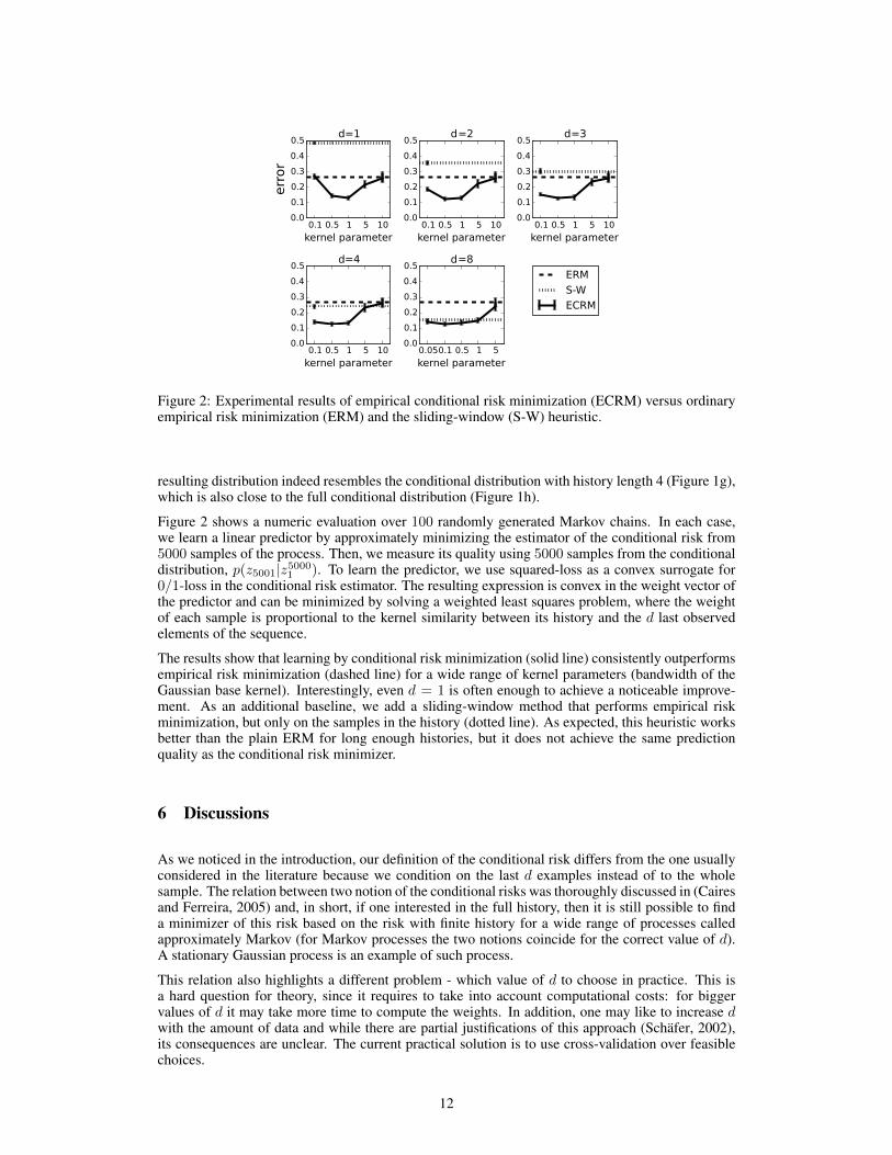
(a) Generating Markov Process (b) Sample sequence, z10001 (c) Contribution of each point tothe conditional risk estimate

(d) p(zN+1) (e) p(zn+1|znn−1) (f) p(zn+1|znn−2) (g) p(zn+1|znn−4) (h) p(zn+1|zn1 )

Figure 1: Illustration of the data distributions in Section 5 by their y-expectations. (a): limit distri-bution of the hidden Markov chain. (b)–(d): conditional distributions of the (n+1)-th sample withhistory lengths 1, 2 and 4. (e): conditional distribution of the (n+1)-th sample with full history.

5 Simulations

This section illustrates the problem setting and the proposed estimator of the conditional risk in asynthetic setting that is easy to analyze but difficult to learn for other techniques. Our goal is tohighlight the differences between marginal and conditional risks and between conditioning on thefinite history and full history.

Let Z = X × Y with X = [0, 10] × [0, 10] ∈ R2 and Y = {±1}. We generate data using a time-homogeneous hidden Markov process with four latent states (Figure 1a). Each state, i, is associatedwith an emission probability distribution, µi(x, y), that is uniform in x and deterministic in y, withy = sign fi(x) for an affine function fi. At any step, i, we observe a sample zi = (xi, yi) from thedistribution associated with the current latent state si. Figure 1b depicts the situation for N = 1000.

Drawn without order, the empirical distribution of the samples zN1 resembles the limit distributionof the hidden Markov chain (Figure 1d), which is also the marginal distribution of the next sam-ple, p(zN+1). Using the dependencies in the sequence, however, we can obtain a more informedestimate, p(zN+1|zN1 ) or its finite history counterparts, p(zN+1|zNN−d) for any history length d.Figures 1e to 1h visualize these distribution: already with a short history length, the conditional dis-tribution is easier learnable (has a lower Bayes risk) than the marginal one. Thus, identifying a goodclassifier for the conditional distribution at each step, i.e. minimizing the conditional risk, can leadto an overall lower error rate than finding a single predictor that is optimal for the limit distribution,i.e. minimizing the marginal risk.

We illustrate the proposed kernel-based estimator of the conditional risk, for d = 4 and a stratifiedset kernel, K(S, S) = 1

2|S+||S+|∑

(i,j)∈S+×S+k(xi, xj) + 1

2|S−||S−|∑

(i,j)∈S−×S− k(xi, xj), for

S = {(xl, yl)}dl=1 and S = {(xl, yl}dl=1, where S+/S− are the sets of positive/negative examples inS (and analogously for S). As base kernel, k(x, x) we use the squared exponential kernel. Figure 1cdepicts the same samples, zN1 , as Figure 1a, but each point zj is drawn at a size proportionally toits contribution to the conditional risk estimate at time N = 1001 for d = 4, i.e. its kernel weightK(zj−1

j−d, zNN+1−d), The points of the history zNN−3 are marked with crosses. One can see that the

11

d d d

d d

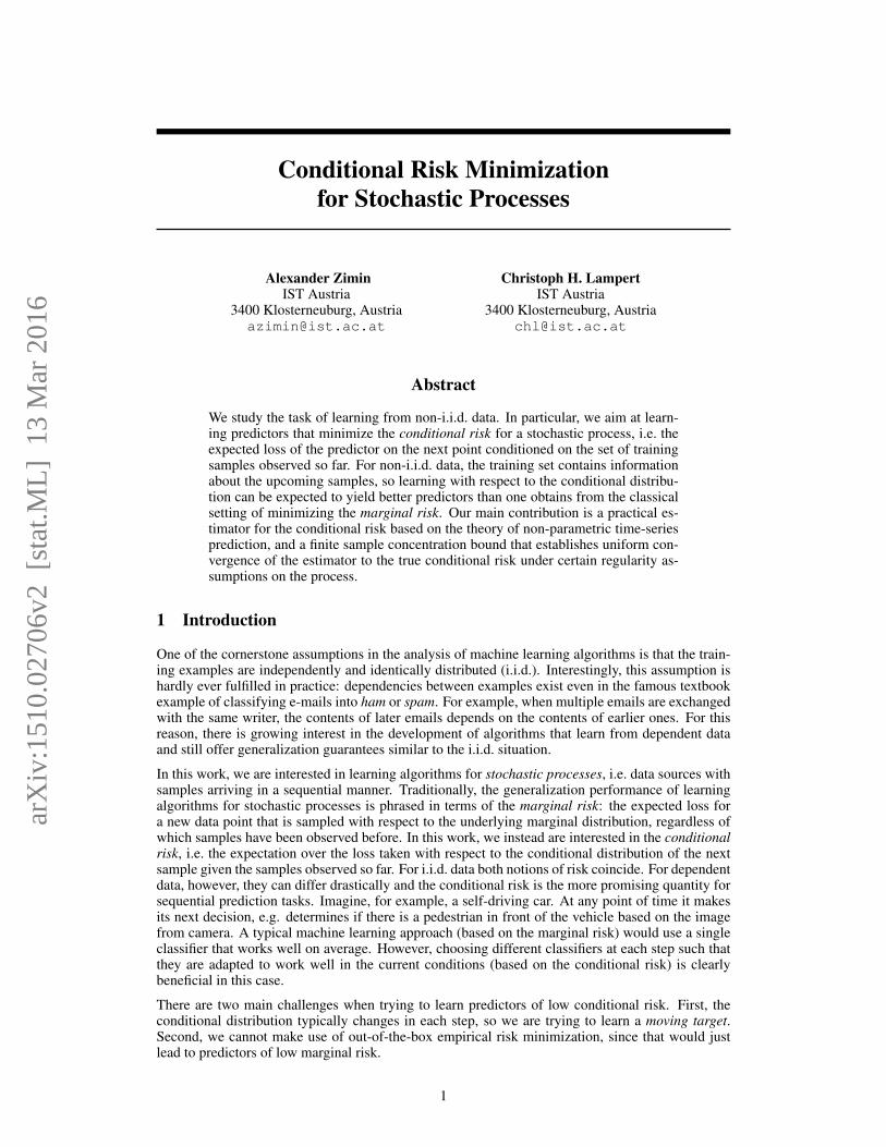
Figure 2: Experimental results of empirical conditional risk minimization (ECRM) versus ordinaryempirical risk minimization (ERM) and the sliding-window (S-W) heuristic.

resulting distribution indeed resembles the conditional distribution with history length 4 (Figure 1g),which is also close to the full conditional distribution (Figure 1h).

Figure 2 shows a numeric evaluation over 100 randomly generated Markov chains. In each case,we learn a linear predictor by approximately minimizing the estimator of the conditional risk from5000 samples of the process. Then, we measure its quality using 5000 samples from the conditionaldistribution, p(z5001|z5000

1 ). To learn the predictor, we use squared-loss as a convex surrogate for0/1-loss in the conditional risk estimator. The resulting expression is convex in the weight vector ofthe predictor and can be minimized by solving a weighted least squares problem, where the weightof each sample is proportional to the kernel similarity between its history and the d last observedelements of the sequence.

The results show that learning by conditional risk minimization (solid line) consistently outperformsempirical risk minimization (dashed line) for a wide range of kernel parameters (bandwidth of theGaussian base kernel). Interestingly, even d = 1 is often enough to achieve a noticeable improve-ment. As an additional baseline, we add a sliding-window method that performs empirical riskminimization, but only on the samples in the history (dotted line). As expected, this heuristic worksbetter than the plain ERM for long enough histories, but it does not achieve the same predictionquality as the conditional risk minimizer.

6 Discussions

As we noticed in the introduction, our definition of the conditional risk differs from the one usuallyconsidered in the literature because we condition on the last d examples instead of to the wholesample. The relation between two notion of the conditional risks was thoroughly discussed in (Cairesand Ferreira, 2005) and, in short, if one interested in the full history, then it is still possible to finda minimizer of this risk based on the risk with finite history for a wide range of processes calledapproximately Markov (for Markov processes the two notions coincide for the correct value of d).A stationary Gaussian process is an example of such process.

This relation also highlights a different problem - which value of d to choose in practice. This isa hard question for theory, since it requires to take into account computational costs: for biggervalues of d it may take more time to compute the weights. In addition, one may like to increase dwith the amount of data and while there are partial justifications of this approach (Schafer, 2002),its consequences are unclear. The current practical solution is to use cross-validation over feasiblechoices.

12

Another important parameter we need to choose is the bandwidth b. Its choice is a known problemfor the kernel estimators themselves. The usual solution is cross-validation, see (Gyorfi et al., 1989)for more details. The proof of validity for such procedure in our setting is possible future work.

With all its benefits, the conditional risk minimization comes with the downside that it requires anintensive computation at each time step. Usually, the amount of computations for a single kernel islinear in d, meaning that it takesO(dN) to compute the weights, and if d is proportional toN , it maybecome quadratic. Afterwards, one also has to perform the optimization itself. While reducing theoptimization costs is an algorithm-dependent problem, it may be possible to optimize computationof weights by some iterative procedure exploiting the fact that the finite history zNN−d+1 changesonly by one point at each step.

Our approach inherits the main problem of nonparametric methods – the curse of dimensionality.For high-dimensional spaces this makes it even harder to consider longer history because of thecomputational consideration above. We believe that in practice this effect can be mitigated by anappropriate choice of the kernel function.

7 Conclusion and possible extensions

In this paper we introduced an empirical estimator of the conditional risk for vector-valued stochasticprocesses and we proved concentration bounds showing that the estimator converges uniformly tothe true risk for large classes at an exponential rate, if the process is β-mixing with sufficiently fastrates.

It is possible to generalize our results in several ways. The stationarity assumption is not essential inour proofs and can be relaxed to conditionally stationary processes from (Caires and Ferreira, 2005).In this case smoothness and robustness will have to be assumed for each time step.

The assumption of the support to be a hypercube was also made for convenience and it can easilybe any compact set. It also can be relaxed by different means. For example, we could make ad-ditional assumptions on the moments of q and p or restrict the supremum over histories to the set{z : ‖z‖ ≤ cn}, with cn increasing as n grows like it was done in (Hansen, 2008). This would leadto a slower convergence rate, though. Another option is to assume that the distribution of zd+1

1 istight, meaning that for every ε > 0 there is a compact setKε such that the probability mass assignedto Kc

ε is less than ε. This approach would require the knowledge of behavior of the covering num-bers of the sets Kε. While all these extension may allow to include more ”real life” distributions, itis more of a technical contribution.

While β-mixing assumption covers a wide range of stochastic processes considered in the literature,there are other dependency measures that may be more suitable for concrete situations. It should bepossible to extend our results to these cases as long as a particular dependency measure allows foruniform convergence of the empirical averages.

References

Adams, T. M. and Nobel, A. B. (2010). Uniform convergence of Vapnik-Chervonenkis classes underergodic sampling. Annals of Probability, 38(4):1345–1367.

Agarwal, A. and Duchi, J. C. (2013). The generalization ability of online algorithms for dependentdata. IEEE Transactions on Information Theory, 59(1):573–587.

Alquier, P. and Wintenberger, O. O. (2012). Model selection for weakly dependent time seriesforecasting. Bernoulli, 18(3):883–913.

Athreya, K. B. and Pantula, S. G. (1986). Mixing properties of Harris chains and autoregressiveprocesses. Journal of Applied Probability, pages 880–892.

Berti, P. and Rigo, P. (1997). A Glivenko-Cantelli theorem for exchangeable random variables.Statistics & Probability Letters, 32(4):385–391.

Biau, G., Bleakley, K., Gyorfi, L., and Ottucsak, G. (2010). Nonparametric sequential prediction oftime series. Journal of Nonparametric Statistics, 22(3):297–317.

13

Bradley, R. C. (2005). Basic properties of strong mixing conditions. A survey and some openquestions. Probability Surveys, 2:107–144.

Caires, S. and Ferreira, J. (2005). On the non-parametric prediction of conditionally stationarysequences. Statistical inference for stochastic processes, 8(2):151–184.

Chen, X., Hansen, L. P., and Carrasco, M. (2010). Nonlinearity and temporal dependence. Journalof Econometrics, 155(2):155–169.

Collomb, G. (1984). Proprietes de convergence presque complete du predicteur a noyau. Zeitschriftfur Wahrscheinlichkeitstheorie und verwandte Gebiete, 66(3):441–460.

Gamarnik, D. (2003). Extension of the PAC framework to finite and countable Markov chains. IEEETransactions on Information Theory, 49(1):338–345.

Gyorfi, L., Hardle, W., Sarda, P., and Vieu, P. (1989). Nonparametric curve estimation from timeseries, volume 60. Springer-Verlag Berlin.

Gyorfi, L., Krzyzak, A., Kohler, M., and Walk, H. (2002). A distribution-free theory of nonparamet-ric regression. Springer.

Gyorfi, L. and Lugosi, G. (1992). Kernel density estimation from ergodic sample is not universallyconsistent. Computational statistics & data analysis, 14(4):437–442.

Hansen, B. E. (2008). Uniform convergence rates for kernel estimation with dependent data. Econo-metric Theory, 24(03):726–748.

Karandikar, R. L. and Vidyasagar, M. (2002). Rates of uniform convergence of empirical meanswith mixing processes. Statistics & Probability Letters, 58(3):297–307.

Kuznetsov, V. and Mohri, M. (2014). Generalization bounds for time series prediction with non-stationary processes. In Algorithmic Learning Theory (ALT), pages 260–274. Springer.

Kuznetsov, V. and Mohri, M. (2015). Learning theory and algorithms for forecasting non-stationarytime series. In Conference on Neural Information Processing Systems (NIPS), pages 541–549.

Meir, R. (2000). Nonparametric time series prediction through adaptive model selection. MachineLearning, 39(1):5–34.

Modha, D. S. and Masry, E. (1996). Minimum complexity regression estimation with weakly de-pendent observations. IEEE Transactions on Information Theory, 42(6):2133–2145.

Modha, D. S. and Masry, E. (1998). Memory-universal prediction of stationary random processes.IEEE Transactions on Information Theory, 44(1):117–133.

Mohri, M. and Rostamizadeh, A. (10 Oct 2013). Stability bounds for stationary ϕ-mixing andβ-mixing processes. http://www.cs.nyu.edu/~mohri/pub/niidj.pdf.

Mohri, M. and Rostamizadeh, A. (2009). Rademacher complexity bounds for non-iid processes. InConference on Neural Information Processing Systems (NIPS), pages 1097–1104.

Pestov, V. (2010). Predictive PAC learnability: A paradigm for learning from exchangeable inputdata. In IEEE International Conference on Granular Computing (GrC), pages 387–391.

Schafer, D. (2002). Strongly consistent online forecasting of centered gaussian processes. IEEETransactions on Information Theory, 48(3):791–799.

Shalizi, C. and Kontorovitch, A. (2013). Predictive PAC learning and process decompositions. InConference on Neural Information Processing Systems (NIPS), pages 1619–1627.

Steinwart, I. and Christmann, A. (2009). Fast learning from non-iid observations. In Conference onNeural Information Processing Systems (NIPS), pages 1768–1776.

Vapnik, V. and Chervonenkis, A. (1971). On the uniform convergence of relative frequencies ofevents to their probabilities. Theory of Probability & Its Applications, 16(2):264–280.

14

Vapnik, V. N. (1998). Statistical learning theory, volume 1. Wiley New York.

Wintenberger, O. (2014). Optimal learning with Bernstein online aggregation. arXiv preprintarXiv:1404.1356.

Yu, B. (1994). Rates of convergence for empirical processes of stationary mixing sequences. Annalsof Probability, pages 94–116.

Zou, B., Li, L., and Xu, Z. (2009). The generalization performance of ERM algorithm with stronglymixing observations. Machine Learning, 75(3):275–295.

15