Conductance Quantization and Landauer Formula

Nina Leonhard SS 2010

1. Important length scales

2. Potential well

3. 2-dimensional electron gas

4. Landauer formula

5. Landauer-Büttiker formalism

6. S-Matrix

Contents

1. Important length scales

2. Potential well

3. 2-dimensional electron gas

4. Landauer formula

5. Landauer-Büttiker formalism

6. S-Matrix

Contents

Important length scales

• Wavelength: at low temperatures current transport occurs for electrons with energies near the Fermi-energy. The Fermi-wavelength is given as:

𝜆𝐹 =2𝜋

𝑘𝐹 𝐸𝐹 =

ℏ2𝑘𝐹2

2𝑚

For low temperatures, meaning 𝑘𝑇 ≪ 𝐸𝐹 , the Fermi distribution is almost a step function

E

f(E)

GaAs: 𝜆𝐹 ≈ 40 nm Si: 𝜆𝐹≈ 35 - 112 nm

𝑘𝑥

𝑘𝑦

𝑘𝐹

−𝑘𝐹

−𝑘𝐹

𝑘𝐹

Important length scales

• Wavelength: at low temperatures current transport occurs for electrons with energies near the Fermi-energy. The Fermi-wavelength is given as:

𝜆𝐹 =2𝜋

𝑘𝐹 𝐸𝐹 =

ℏ2𝑘𝐹2

2𝑚

For low temperatures, meaning 𝑘𝑇 ≪ 𝐸𝐹 , the Fermi distribution is almost a step function

E

f(E)

GaAs: 𝜆𝐹 ≈ 40 nm Si: 𝜆𝐹≈ 35 - 112 nm

Important length scales

• Mean free path 𝑳𝒎: distance an electron travels until its initial momentum is destroyed

• Phase-relaxation length 𝑳𝝋: distance an electron travels until its initial

phase is randomized

Ballistic regime: 𝜆𝐹 < 𝐿 < 𝐿𝑚 Diffusive regime 𝐿 > 𝐿𝑚 Coherent transport: 𝐿 < 𝐿𝜑 Incoherent transport: 𝐿 > 𝐿𝜑

GaAs: 𝐿𝑚 ≈ 100 − 10000 nm 𝐿𝜑 ≈ 200 nm

Si : 𝐿𝑚 ≈ 37 − 118 nm 𝐿𝜑 ≈ 40 − 400 nm

𝑳𝒎

𝑳𝝋

1. Important length scales

2. Potential well

3. 2-dimensional electron gas

4. Landauer formula

5. Landauer-Büttiker formalism

6. S-Matrix

Contents

Solve

−ℏ2

2𝑚∆ + 𝑉 𝑥 Ψ 𝑥 = 𝐸Ψ 𝑥

with boundary conditions

Ψ −𝐿

2= Ψ +

𝐿

2= 0

⇒ 𝐸𝑛 =ℏ2𝜋2𝑛2

2𝑚𝐿2

𝑘𝑛 =𝑛𝜋

𝐿

with 𝑛 ∈ ℕ

Number of occupied states

𝐸𝐹 =ℏ2𝑘𝐹2

2𝑚= 𝐸𝑀 =

ℏ2𝜋2𝑀2

2𝑚𝐿2

⇒ 𝑀 = 𝐼𝑛𝑡𝑘𝐹𝐿

π

Potential well

E

L

Potential well

Discrete energy-levels for small widths For macroscopic systems energy bands

E E

1. Important length scales

2. Potential well

3. 2-dimensional electron gas

4. Landauer formula

5. Landauer-Büttiker formalism

6. S-Matrix

Contents

Two semiconductor layers:

n-AlGaAs and i-GaAs layer

electrons flow from n- to i-layer

electrons are „caught“ in z-direction

2-dimensional electron gas

z

z

𝐸𝐶

𝐸𝐶

𝐸𝐹

𝐸𝐹

𝐸𝑉

𝐸𝑉

E

E

2-deg

Wavefunction of a free particle

Ψ 𝑥, 𝑦, 𝑧 = 𝜙𝑚 𝑧 𝑒𝑖𝑘𝑥𝑥𝑒𝑖𝑘𝑦𝑦

Its energy is given as:

𝐸(𝑘) = 𝐸𝐶 + 𝜀𝑚(𝑧) +ℏ2

2𝑚𝑘𝑥2 + 𝑘𝑦

2

𝜀𝑚(𝑧): transverse energy in z-direction

2-deg: only 𝑚 = 1 is occupied

𝜀1(𝑧) < 𝐸𝐹 𝜀𝑚>1

(𝑧) > 𝐸𝐹

2-dimensional electron gas

𝑘 = 𝑘𝑥2 + 𝑘𝑦

2

E(k)

𝐸𝐹

𝜀1(𝑧)

𝜀2(𝑧)

𝜀3(𝑧)

2-dimensional electron gas

contact 1 contact 2 L

W

Ohm‘s law for the resistance 𝑅 =𝐿

𝜎𝑊

We can also use the conductance 𝐺 = 𝑅−1 =σ𝑊

𝐿

For 𝐿 → 0 we would expect 𝐺 → ∞

But: experiments show that G is quantized

𝑊 ≪ 𝐿 𝑘𝐹 < 𝐿 < 𝐿𝑚

x

y

2-dimensional electron gas

First experimental results were obtained by B.J. van Wees in 1988

2-dimensional electron gas at an AlGaAs-GaAs interface

The width is controlled with the gate voltage

Width

2-dimensional electron gas

𝐸𝐹

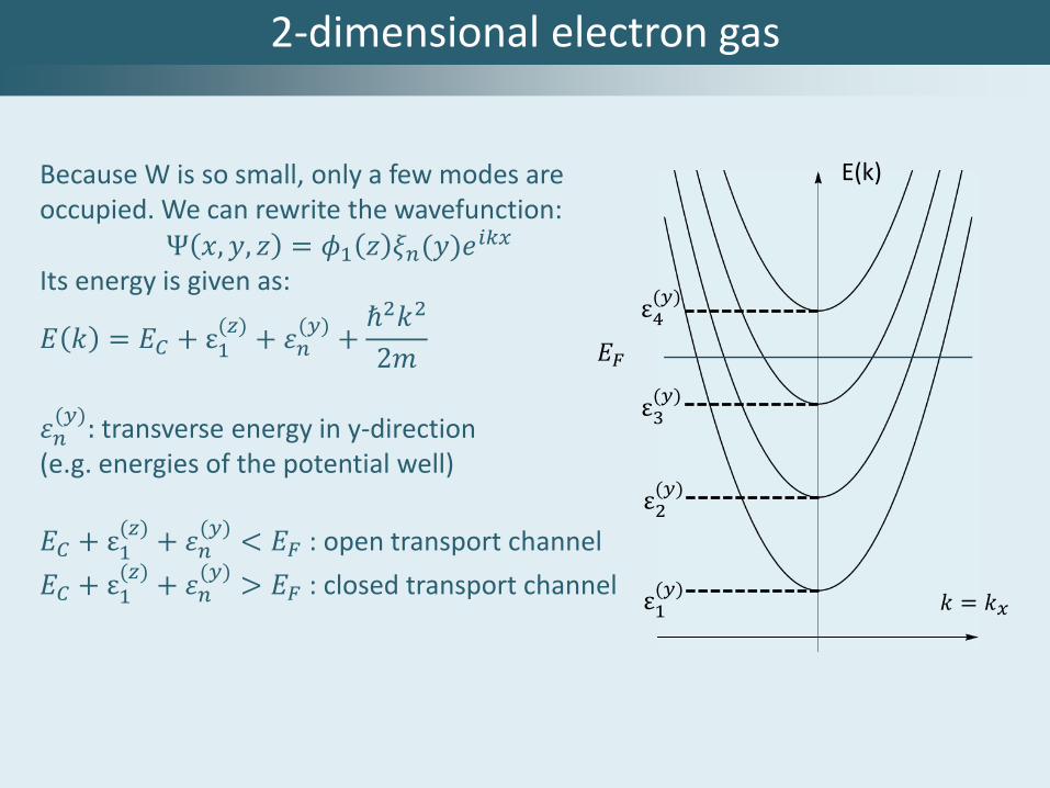
Because W is so small, only a few modes are occupied. We can rewrite the wavefunction:

Ψ 𝑥, 𝑦, 𝑧 = 𝜙1 𝑧 𝜉𝑛(𝑦)𝑒𝑖𝑘𝑥

Its energy is given as:

𝐸 𝑘 = 𝐸𝐶 + ε1(𝑧)+ 𝜀𝑛(𝑦)+ℏ2𝑘2

2𝑚

𝜀𝑛(𝑦): transverse energy in y-direction

(e.g. energies of the potential well)

𝐸𝐶 + ε1(𝑧)+ 𝜀𝑛(𝑦)< 𝐸𝐹 : open transport channel

𝐸𝐶 + ε1(𝑧)+ 𝜀𝑛(𝑦)> 𝐸𝐹 : closed transport channel

𝑘 = 𝑘𝑥

E(k)

ε1(𝑦)

ε2(𝑦)

ε3(𝑦)

ε4(𝑦)

1. Important length scales

2. Potential well

3. 2-dimensional electron gas

4. Landauer formula

5. Landauer-Büttiker formalism

6. S-Matrix

Contents

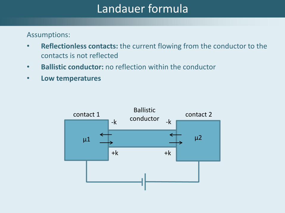
Landauer formula

Assumptions:

• Reflectionless contacts: the current flowing from the conductor to the contacts is not reflected

• Ballistic conductor: no reflection within the conductor

• Low temperatures

contact 1 contact 2 Ballistic

conductor

µ1 µ2

-k -k

+k +k

Landauer formula

Result: finite contact resistance that is quantized for a ballistic

conductor 𝐺𝐶 =2𝑒2

ℎ𝑀

How do we calculate M?

Number of modes can be estimated to be (for zero magnetic field)

𝑀 = 𝐼𝑛𝑡𝑘𝐹𝑊

π

because of 𝐸𝑀 = 𝐸𝐹

Landauer formula

A very large number of modes has to be carried by a few modes.

k k k

E E E

resistance = contact resistance

𝜇1

𝜇2 𝜇2

𝜇1

Landauer formula

Now consider a conductor with two ballistic leads. There is a

transmission probability T that an electron crosses the conductor.

𝐼1+ =2𝑒

ℎ𝑀[μ1 − 𝜇2] and 𝐼2

+ =2𝑒

ℎ𝑀𝑇 μ1 − 𝜇2

𝐼1− =2𝑒

ℎ𝑀(1 − 𝑇)[μ1 − 𝜇2]

Total current: 𝐼 = 𝐼1+ − 𝐼1

− = 𝐼2+ =2𝑒

ℎ𝑀𝑇 𝜇1 − 𝜇2 ⇒ 𝐺 =

2𝑒2

ℎ𝑀𝑇

µ1 µ2 Lead 1 Lead 2 conductor

𝐼1+

𝐼1−

𝐼2+

transmission

reflection

Landauer formula

𝐺 =2𝑒2

ℎ𝑀𝑇 Landauer formula

Generalization: 𝐺 =2𝑒2

ℎ 𝑀𝑇𝑛 𝑛

Can we obtain Ohm‘s law from the Landauer formula? Yes, we can see that:

𝐺−1 =𝐿

σ𝑊+𝐿0σ𝑊

1. Important length scales

2. Potential well

3. 2-dimensional electron gas

4. Landauer formula

5. Landauer-Büttiker formalism

6. S-Matrix

Contents

Landauer-Büttiker-formalism

More difficult problem, e.g.

1

2

3

V

Landauer-Büttiker-formalism

The formula has to be modified

𝐼𝑝 =2𝑒

ℎ 𝑇𝑞←𝑝𝜇𝑝 − 𝑇𝑝←𝑞μ𝑞𝑞 with 𝑇 = 𝑀𝑇

We can introduce 𝐺𝑝𝑞 =2𝑒2

ℎ𝑇𝑝←𝑞

and obtain

𝐼𝑝= 𝐺𝑝𝑞𝑉𝑝 − 𝐺𝑞𝑝𝑉𝑞𝑞

Sum rule (Kirchhoff-laws):

𝐺𝑞𝑝𝑞 = 𝐺𝑝𝑞𝑞

1. Important length scales

2. Potential well

3. 2-dimensional electron gas

4. Landauer formula

5. Landauer-Büttiker formalism

6. S-Matrix

Contents

S-Matrix

For a coherent conductor the transmission function can be expressed with the scattering matrix. The scattering matrix relates the incoming amplitudes for each state with the outgoing amplitudes after the scattering process.

𝑏 = 𝑆 𝑎 For the transmission probabilities:

𝑇𝑚←𝑛 = 𝑠𝑚←𝑛

2

𝑆 = 𝑟 𝑡′𝑡 𝑟′

𝑟, 𝑡, 𝑟‘, 𝑡‘ are matrices

Incoming states {a}

µ1 µ2

{b} states after scattering

Scattering

S

S-Matrix

Properties of the S-matrix: • Calculating the S-matrix is equivalent to solving the problem. • dim𝑆 = 𝑀𝑇 ×𝑀𝑇 with 𝑀𝑇(𝐸) = 𝑀𝑝(𝐸)𝑝

• S has to be unitary 𝑆†S = 𝑆𝑆† = 𝐼 • Reversing the magnetic field transposes the S-Matrix

𝑆 𝐵 = 𝑆𝑡(−𝐵)

S-Matrix

Combining S-matrices: Instead of solving the problem rightaway, one can divide it into smaller problems that have already been solved. Example:

𝑎1

𝑎3 𝑏1

𝑏3 𝑏2

𝑎2

𝐬(𝟏) 𝐬(𝟐)

S-Matrix

𝑏1𝑏2= 𝑟

(1) 𝑡′(1)

𝑡(1) 𝑟′(1)𝑎1𝑎2 and

𝑏3𝑎2= 𝑟

(2) 𝑡′(2)

𝑡(2) 𝑟′(2)𝑎3𝑏2

Eliminate 𝑎2 and 𝑏2: 𝑏1𝑏3=𝑟 𝑡′

𝑡 𝑟′𝑎1𝑎3

Where 𝑡 = 𝑡(2)𝑡(1)

1−𝑟′(1)𝑟(2)

𝑡′ =𝑡′(1)𝑡′(2)

1−𝑟(2)𝑟′(1)

𝑟 = 𝑟(1) +𝑡′(1)𝑟(2)𝑡(1)

1−𝑟′(1)𝑟(2)

𝑟′ = 𝑟′ 2 +𝑡(2)𝑟′(1)𝑡′(2) 1−𝑟′(1)𝑟(2)

𝑠(1)

𝑠(2)

𝑠(1+2)

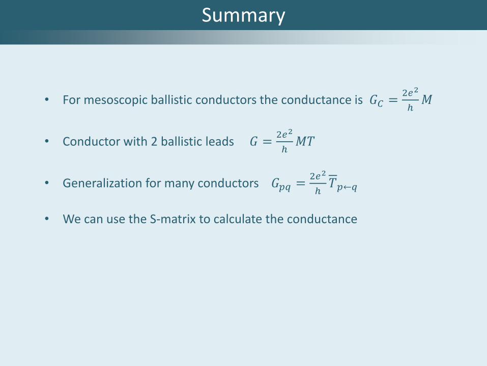
Summary

• For mesoscopic ballistic conductors the conductance is 𝐺𝐶 =2𝑒2

ℎ𝑀

• Conductor with 2 ballistic leads 𝐺 =2𝑒2

ℎ𝑀𝑇

• Generalization for many conductors 𝐺𝑝𝑞 =2𝑒2

ℎ𝑇𝑝←𝑞

• We can use the S-matrix to calculate the conductance

Thank you for your attention.