Conference on PDE Methods in Applied Mathematics and Image Processing, Sunny Beach, Bulgaria, 2004 NUMERICAL APPROACH IN SOLVING THE PDE FOR PARTICULAR FLUID DYNAMICS CASES Zoran Markov Faculty of Mechanical Engineering University in Skopje, Macedonia Joint research Predrag Popovski University in Skopje, Macedonia Andrej Lipej Turboinstitut, Slovenia
Transcript
Con
fere
nce
on P
DE
Met
hods
in A
ppli
ed M
athe
mat
ics
and
Imag
e P
roce
ssin
g, S
unny
Bea
ch, B
ulga
ria,
200
4
NUMERICAL APPROACH IN SOLVING THE PDE FOR PARTICULAR FLUID DYNAMICS
CASES
Zoran Markov Faculty of Mechanical Engineering
University in Skopje, Macedonia
Joint research Predrag Popovski
University in Skopje, Macedonia
Andrej Lipej Turboinstitut, Slovenia
Z. Markov: NUMERICAL APPROACH IN SOLVING THE PDE FOR PARTICULAR FLUID DYNAMICS CASES
Con
fere
nce
on P
DE
Met
hods
in A
ppli
ed M
athe
mat
ics
and
Imag
e P
roce
ssin
g, S
unny
Bea
ch, B
ulga
ria,
200
4
2
Overview
• INTRODUCTION
• NUMERICAL MODELING AND GOVERNING EQUATIONS
• TURBULENCE MODELING
• VERIFICATION OF THE NUMERICAL RESULTS USING EXPERIMENTAL DATA
Z. Markov: NUMERICAL APPROACH IN SOLVING THE PDE FOR PARTICULAR FLUID DYNAMICS CASES
Con
fere
nce
on P
DE
Met
hods
in A
ppli
ed M
athe
mat
ics
and
Imag
e P
roce
ssin
g, S
unny
Bea
ch, B
ulga
ria,
200
4
3
1. Introduction
• Solving the PDE equations in fluid dynamics has proved difficult, even impossible in some cases
• Development of numerical approach was necessary in the design of hydraulic machinery
• Greater speed of the computers and development of reliable software
• Calibration and verification of all numerical models is an iterative process
Z. Markov: NUMERICAL APPROACH IN SOLVING THE PDE FOR PARTICULAR FLUID DYNAMICS CASES
Con
fere
nce
on P
DE
Met
hods
in A
ppli
ed M
athe
mat
ics
and
Imag
e P
roce
ssin
g, S
unny
Bea
ch, B
ulga
ria,
200
4
4
2. Numerical Modeling and Governing Equations
• Continuity and Momentum Equations
• Compressible Flows
• Time-Dependent Simulations
Z. Markov: NUMERICAL APPROACH IN SOLVING THE PDE FOR PARTICULAR FLUID DYNAMICS CASES
Con
fere
nce
on P
DE
Met
hods
in A
ppli
ed M
athe
mat
ics
and
Imag
e P
roce
ssin
g, S
unny
Bea
ch, B
ulga
ria,
200
4
5
2.1. Continuity and Momentum Equations
• The Mass Conservation Equation
• Momentum Conservation Equations
( ) ( ) iji i j i i
j i j
pu u u g F
t x x x
2
3ji l
ij ijj i l
uu u
x x x
i-direction in a internal (non-accelerating) reference frame:
mii
Suxt
Z. Markov: NUMERICAL APPROACH IN SOLVING THE PDE FOR PARTICULAR FLUID DYNAMICS CASES
Con
fere
nce
on P
DE
Met
hods
in A
ppli
ed M
athe
mat
ics
and
Imag
e P
roce
ssin
g, S
unny
Bea
ch, B
ulga
ria,
200
4
6
2.2. Compressible Flows
When to Use the Compressible Flow Model? M<0.1 - subsonic, compressibility effects are negligible M1- transonic, compressibility effects become important M>1- supersonic, may contain shocks and expansion fans, which
can impact the flow pattern significantly
Physics of Compressible Flows total pressure and total temperature :
120 1
12s
pM
p
211
2o
s
TM
T
The Compressible Form of Gas Law ideal gas law: ( ) /op sp p RT
Z. Markov: NUMERICAL APPROACH IN SOLVING THE PDE FOR PARTICULAR FLUID DYNAMICS CASES
Con
fere
nce
on P
DE
Met
hods
in A
ppli
ed M
athe
mat
ics
and
Imag
e P
roce
ssin
g, S
unny
Bea
ch, B
ulga
ria,
200
4
7
2.3. Time-Dependent Simulations
Temporal Discretization
Time-dependent equations must be discretized in both space and time
A generic expressions for the time evolution of a variable is given by
( )Ft
1
( )n n
Ft
1 13 4( )
2
n n n
Ft
where the function F incorporates any spatial discretization If the time derivative is discretized using backward differences, the first-order accurate temporal discretization is
given by
second-order discretization is given by
Z. Markov: NUMERICAL APPROACH IN SOLVING THE PDE FOR PARTICULAR FLUID DYNAMICS CASES
Con
fere
nce
on P
DE
Met
hods
in A
ppli
ed M
athe
mat
ics
and
Imag
e P
roce
ssin
g, S
unny
Bea
ch, B
ulga
ria,
200
4
8
3. Turbulence Modeling
Standard CFD codes usually provide the following choices of turbulence models:
Spalart-Allmaras model• Standard k- model• Renormalization-group (RNG) k- model• Realizable k- model Reynolds stress model (RSM) Large eddy simulation (LES) model
Z. Markov: NUMERICAL APPROACH IN SOLVING THE PDE FOR PARTICULAR FLUID DYNAMICS CASES
Con
fere
nce
on P
DE
Met
hods
in A
ppli
ed M
athe
mat
ics
and
Imag
e P
roce
ssin
g, S
unny
Bea
ch, B
ulga
ria,
200
4
9
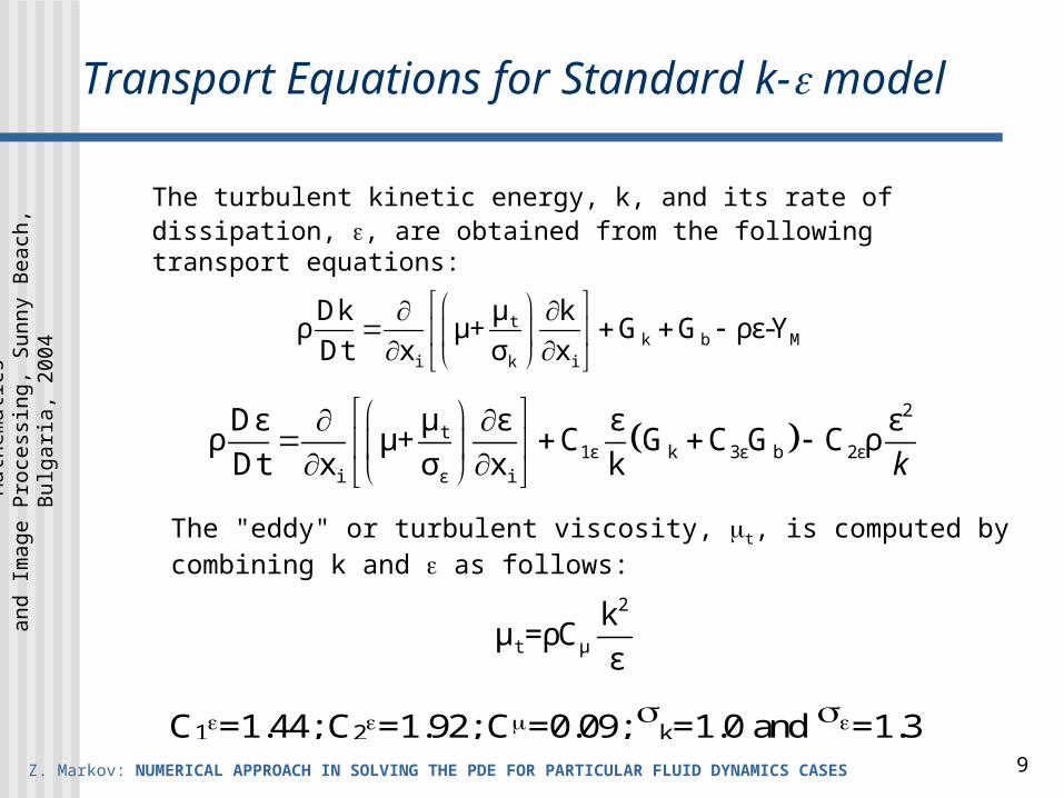
Transport Equations for Standard k- model
tk b M
i k i
μDk kρ μ+ G G ρε-Y
Dt x σ x
The turbulent kinetic energy, k, and its rate of dissipation, , are obtained from the following transport equations:
2
t1ε k 3ε b 2ε
i ε i
μDε ε ε ερ μ+ C G C G C ρ
Dt x σ x k k
2
t μ
kμ =ρC
ε
The "eddy" or turbulent viscosity, t, is computed by combining k and as follows:
C1=1.44; C2=1.92; C=0.09; k=1.0 and =1.3
Z. Markov: NUMERICAL APPROACH IN SOLVING THE PDE FOR PARTICULAR FLUID DYNAMICS CASES
Con
fere
nce
on P
DE
Met
hods
in A
ppli
ed M
athe
mat
ics
and
Imag
e P
roce
ssin
g, S
unny
Bea
ch, B
ulga
ria,
200
4
10
4. Verification Of The Numerical Results Using Experimental Data
• Simulation of Projectile Flight Dynamics
• Hydrodynamic and Cavitation Performances of Modified NACA Hydrofoil
• Cavitation Performances of Pump-turbine
Z. Markov: NUMERICAL APPROACH IN SOLVING THE PDE FOR PARTICULAR FLUID DYNAMICS CASES
Con
fere
nce
on P
DE
Met
hods
in A
ppli
ed M
athe
mat
ics
and
Imag
e P
roce
ssin
g, S
unny
Bea
ch, B
ulga
ria,
200
4
11
4.1. Simulation of Projectile Flight Dynamics
Part/Subassembly: Multiple
Mass: 14.968Kg
Volume: 3140185.9077mm̂3
Centroid: X: 307.1229
Y: 0
Z: 0
Moments of inertia: X: 22273.0654
Y: 1641718.8812
Z: 1641715.2464
Products of inertia: XY: 0
XZ: 0
YZ: 0
Radii of Gyration: X: 38.5752
Y: 331.1828
Z: 331.1824
Principal moments and X-Y-Z directions about centroid:
I: 22273.0654 along [1,0,0]
J : 229871.3222 along [0,1,0]
K: 229867.6875 along [0,0,1]
Projectile 105 mm M1 - mass analysis
Z. Markov: NUMERICAL APPROACH IN SOLVING THE PDE FOR PARTICULAR FLUID DYNAMICS CASES
Con
fere
nce
on P
DE
Met
hods
in A
ppli
ed M
athe
mat
ics
and
Imag
e P
roce
ssin
g, S
unny
Bea
ch, B
ulga
ria,
200
4
12
4.1. Simulation of Projectile Flight Dynamics (2)
Comparison of the projectile trajectory elements obtained as a result of thesimulation with those given in the range tables
Initial conditions:
Elevation angle 0
Muzzle velocity V0
Method forobtaining of the
results
Max
imum
ran
ge[m
]
Tim
e of
fli
ght
[sec
]
Max
imum
heig
ht[m
]
Ang
le o
f im
pact
on t
he g
roun
d[]
Impa
ct v
eloc
ity
[m/s
]
Simulation 3069 12.8 201 15.4 231
Range tables 3100 12.9 203 15.6 233
0 = 14
V0 = 267 m/sError [] 0.1 0.77 0.98 1.28 0.85
Simulation 3568 17.6 381 24.3 205
Range tables 3600 17.7 383 24.6 207
0 = 22
V0 = 238 m/sError [] 0.88 0.56 0.52 1.21 0.96
Simulation 7794 31 1188 34.7 253
Range tables 8100 31.5 1229 35 259
0 = 28
V0 = 376 m/sError [] 1.3 1.58 3.33 0.85 2.31
Z. Markov: NUMERICAL APPROACH IN SOLVING THE PDE FOR PARTICULAR FLUID DYNAMICS CASES
Con
fere
nce
on P
DE
Met
hods
in A
ppli
ed M
athe
mat
ics
and
Imag
e P
roce
ssin
g, S
unny
Bea
ch, B
ulga
ria,
200
4
13
Maximum range comparison
0
2000
4000
6000
8000
10000
10 15 20 25 30
Elevation angle [deg]
Ma
x.
ran
ge
[m
]
Simulation Range tables
4.1. Simulation of Projectile Flight Dynamics (3)
Comparison of the projectile's maximum range
Z. Markov: NUMERICAL APPROACH IN SOLVING THE PDE FOR PARTICULAR FLUID DYNAMICS CASES
Con
fere
nce
on P
DE
Met
hods
in A
ppli
ed M
athe
mat
ics
and
Imag
e P
roce
ssin
g, S
unny
Bea
ch, B
ulga
ria,
200
4
14
4.2. Hydrodynamic and Cavitation Performances of Modified NACA Hydrofoil
cevka
• Modified NACA 4418 Hydrofoil
Z. Markov: NUMERICAL APPROACH IN SOLVING THE PDE FOR PARTICULAR FLUID DYNAMICS CASES
Con
fere
nce
on P
DE
Met
hods
in A
ppli
ed M
athe
mat
ics
and
Imag
e P
roce
ssin
g, S
unny
Bea
ch, B
ulga
ria,
200
4
15
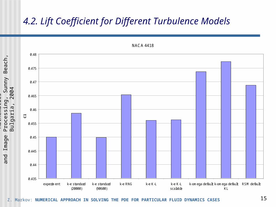
4.2. Lift Coefficient for Different Turbulence Models
NACA 4418
0.435
0.44
0.445
0.45
0.455
0.46
0.465
0.47
0.475
0.48
experiment k-e standard(20000)
k-e standard(90600)
k-e RNG k-e K-L k-e K-Lscalable
k-omega default k-omega defaultKL
RSM default
Cl
Z. Markov: NUMERICAL APPROACH IN SOLVING THE PDE FOR PARTICULAR FLUID DYNAMICS CASES
Con
fere
nce
on P
DE
Met
hods
in A
ppli
ed M
athe
mat
ics
and
Imag
e P
roce
ssin
g, S
unny
Bea
ch, B
ulga
ria,
200
4
16
4.2. Pressure Coefficient Around the Blade With and Without Cavitation
NACA 4418
-5
-4
-3
-2
-1
0
1
2
0.0 0.1 0.2 0.3 0.4 0.5 0.6 0.7 0.8 0.9 1.0
x/L
Cp
exp s2 exp s7 Fluent-s7 Fluent-s2
Z. Markov: NUMERICAL APPROACH IN SOLVING THE PDE FOR PARTICULAR FLUID DYNAMICS CASES
Con
fere
nce
on P
DE
Met
hods
in A
ppli
ed M
athe
mat
ics
and
Imag
e P
roce
ssin
g, S
unny
Bea
ch, B
ulga
ria,
200
4
17
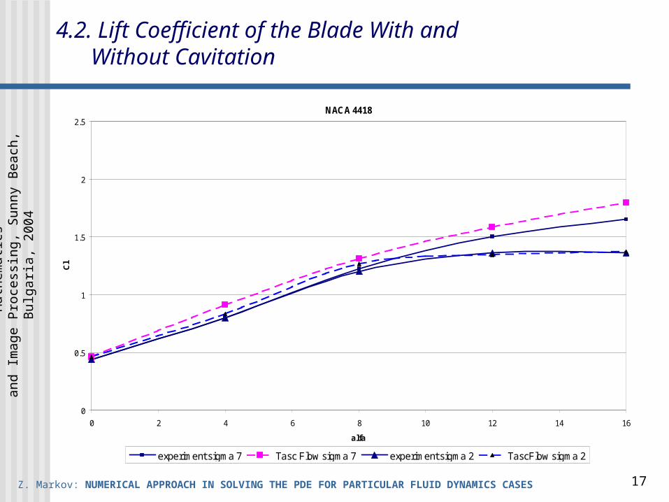
4.2. Lift Coefficient of the Blade With and Without Cavitation