Confessions of an Accidental Benchmarker

1 Confessions of an Accidental Benchmarker

•  Appendix B of the Linpack Users’ Guide •  Designed to help users extrapolate execution time for

Linpack software package •  First benchmark report from 1977;

•  Cray 1 to DEC PDP-10

http://bit.ly/hpcg-benchmark

Jack Dongarra & Piotr Luszczek University of Tennessee Oak Ridge National Laboratory Mike Heroux Sandia National Laboratory

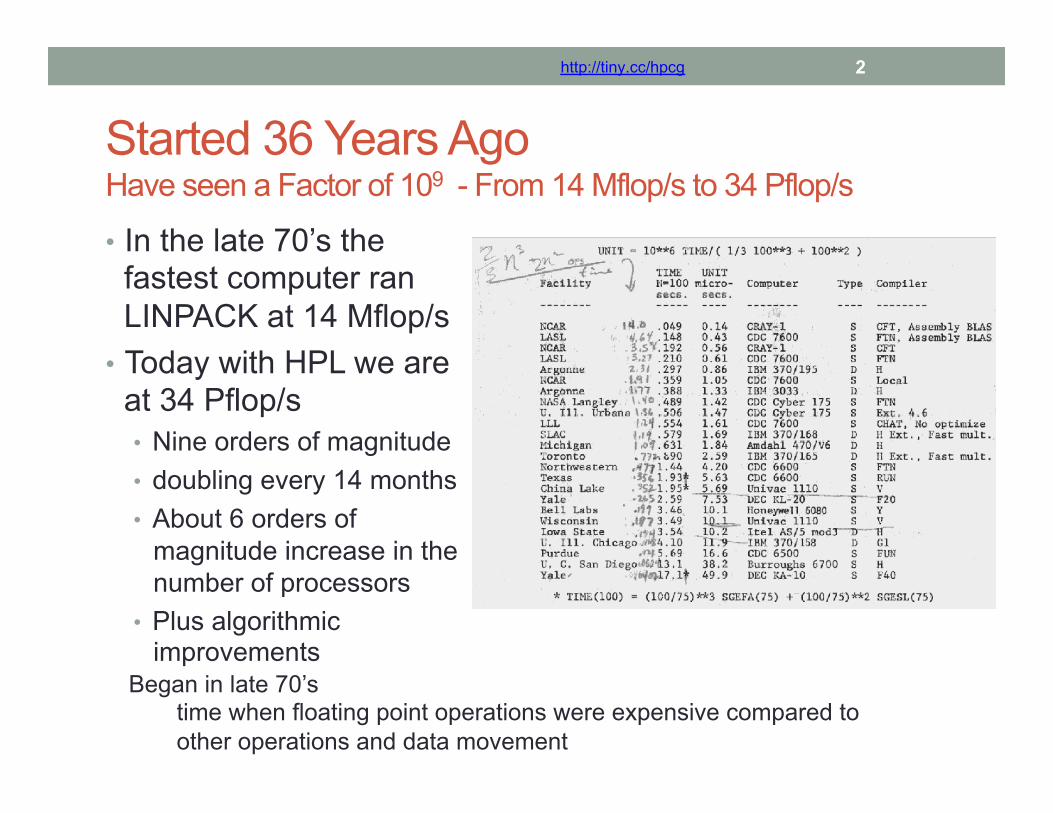
Started 36 Years Ago Have seen a Factor of 109 - From 14 Mflop/s to 34 Pflop/s

•  In the late 70’s the fastest computer ran LINPACK at 14 Mflop/s

•  Today with HPL we are at 34 Pflop/s •  Nine orders of magnitude •  doubling every 14 months •  About 6 orders of

magnitude increase in the number of processors

•  Plus algorithmic improvements

Began in late 70’s time when floating point operations were expensive compared to other operations and data movement

http://tiny.cc/hpcg 2

High Performance Linpack (HPL) •  Is a widely recognized and discussed metric for ranking

high performance computing systems • When HPL gained prominence as a performance metric in

the early 1990s there was a strong correlation between its predictions of system rankings and the ranking that full-scale applications would realize.

• Computer system vendors pursued designs that would increase their HPL performance, which would in turn improve overall application performance.

•  Today HPL remains valuable as a measure of historical trends, and as a stress test, especially for leadership class systems that are pushing the boundaries of current technology.


The Problem • HPL performance of computer systems are no longer so

strongly correlated to real application performance, especially for the broad set of HPC applications governed by partial differential equations.

• Designing a system for good HPL performance can

actually lead to design choices that are wrong for the real application mix, or add unnecessary components or complexity to the system.

http://bit.ly/hpcg-benchmark 4

Concerns •  The gap between HPL predictions and real application

performance will increase in the future. • A computer system with the potential to run HPL at 1

Exaflops is a design that may be very unattractive for real applications.

•  Future architectures targeted toward good HPL performance will not be a good match for most applications.

•  This leads us to a think about a different metric


HPL - Good Things • Easy to run • Easy to understand • Easy to check results • Stresses certain parts of the system • Historical database of performance information • Good community outreach tool •  “Understandable” to the outside world •  If your computer doesn’t perform well on the LINPACK

Benchmark, you will probably be disappointed with the performance of your application on the computer.


HPL - Bad Things •  LINPACK Benchmark is 36 years old

•  Top500 (HPL) is 21 years old

•  Floating point-intensive performs O(n3) floating point operations and moves O(n2) data.

• No longer so strongly correlated to real apps. • Reports Peak Flops (although hybrid systems see only 1/2 to 2/3 of Peak) • Encourages poor choices in architectural features • Overall usability of a system is not measured • Used as a marketing tool • Decisions on acquisition made on one number • Benchmarking for days wastes a valuable resource


Running HPL •  In the beginning to run HPL on the number 1 system

was under an hour. • On Livermore’s Sequoia IBM BG/Q the HPL run took

about a day to run. •  They ran a size of n=12.7 x 106 (1.28 PB)

•  16.3 PFlop/s requires about 23 hours to run!!

•  23 hours at 7.8 MW that the equivalent of 100 barrels of oil or about $8600 for that one run.

•  The longest run was 60.5 hours •  JAXA machine

•  Fujitsu FX1, Quadcore SPARC64 VII 2.52 GHz •  A matrix of size n = 3.3 x 106

•  .11 Pflop/s #160 today


0%#

10%#

20%#

30%#

40%#

50%#

60%#

70%#

80%#

90%#

100%#

6/1/93#

10/1/93#

2/1/94#

6/1/94#

10/1/94#

2/1/95#

6/1/95#

10/1/95#

2/1/96#

6/1/96#

10/1/96#

2/1/97#

6/1/97#

10/1/97#

2/1/98#

6/1/98#

10/1/98#

2/1/99#

6/1/99#

10/1/99#

2/1/00#

6/1/00#

10/1/00#

2/1/01#

6/1/01#

10/1/01#

2/1/02#

6/1/02#

10/1/02#

2/1/03#

6/1/03#

10/1/03#

2/1/04#

6/1/04#

10/1/04#

2/1/05#

6/1/05#

10/1/05#

2/1/06#

6/1/06#

10/1/06#

2/1/07#

6/1/07#

10/1/07#

2/1/08#

6/1/08#

10/1/08#

2/1/09#

6/1/09#

10/1/09#

2/1/10#

6/1/10#

10/1/10#

2/1/11#

6/1/11#

10/1/11#

2/1/12#

6/1/12#

10/1/12#

2/1/13#

6/1/13#

61#hours#

30#hours#

20#hours#

12#hours#

11#hours#

10#hours#

9#hours#

8#hours#

7#hours#

6#hours#

5#hours#

4#hours#

3#hours#

2#hours#

1#hour#

Run Times for HPL on Top500 Systems http://bit.ly/hpcg-benchmark 9

#1 System on the Top500 Over the Past 20 Years (16 machines in that club)

Top500 List Computer r_max

(Tflop/s) n_max Hours MW 6/93 (1) TMC CM-5/1024 .060 52224 0.4 11/93 (1) Fujitsu Numerical Wind Tunnel .124 31920 0.1 1. 6/94 (1) Intel XP/S140 .143 55700 0.2

11/94 - 11/95 (3) Fujitsu Numerical Wind Tunnel .170 42000 0.1 1.

6/96 (1) Hitachi SR2201/1024 .220 138,240 2.2 11/96 (1) Hitachi CP-PACS/2048 .368 103,680 0.6

6/97 - 6/00 (7) Intel ASCI Red 2.38 362,880 3.7 .85 11/00 - 11/01 (3) IBM ASCI White, SP Power3 375 MHz 7.23 518,096 3.6 6/02 - 6/04 (5) NEC Earth-Simulator 35.9 1,000,000 5.2 6.4 11/04 - 11/07

(7) IBM BlueGene/L 478. 1,000,000 0.4 1.4 6/08 - 6/09 (3) IBM Roadrunner –PowerXCell 8i 3.2 Ghz 1,105. 2,329,599 2.1 2.3

11/09 - 6/10 (2) Cray Jaguar - XT5-HE 2.6 GHz 1,759. 5,474,272 17.3 6.9 11/10 (1) NUDT Tianhe-1A, X5670 2.93Ghz NVIDIA 2,566. 3,600,000 3.4 4.0

6/11 - 11/11 (2) Fujitsu K computer, SPARC64 VIIIfx 10,510. 11,870,208 29.5 9.9 6/12 (1) IBM Sequoia BlueGene/Q 16,324. 12,681,215 23.1 7.9 11/12 (1) Cray XK7 Titan AMD + NVIDIA Kepler 17,590. 4,423,680 0.9 8.2

6/13 – 11/13(?) NUDT Tianhe-2 Intel IvyBridge & Xeon Phi 33,862. 9,960,000 5.4 17.8

9 6 2


Ugly Things about HPL • Doesn’t probe the architecture; only one data point • Constrains the technology and architecture options for

HPC system designers. •  Skews system design.

•  Floating point benchmarks are not quite as valuable to some as data-intensive system measurements


Many Other Benchmarks • Top 500 • Green 500 • Graph 500 142 • Sustained Petascale Performance

• HPC Challenge • Perfect • ParkBench • SPEC-hpc

• Livermore Loops • EuroBen • NAS Parallel Benchmarks • Genesis • RAPS • SHOC • LAMMPS • Dhrystone • Whetstone


Proposal: HPCG • High Performance Conjugate Gradient (HPCG). • Solves Ax=b, A large, sparse, b known, x computed. • An optimized implementation of PCG contains essential

computational and communication patterns that are prevalent in a variety of methods for discretization and numerical solution of PDEs

• Patterns:

•  Dense and sparse computations. •  Dense and sparse collective. •  Data-driven parallelism (unstructured sparse triangular solves).

• Strong verification and validation properties (via spectral properties of CG).


What about the NAS Parallel CG Benchmark?

•  NAS CG is flawed from the perspective of modeling the design choices of real science and engineering codes.

•  The matrix truly random and make the placement of entries random means that, for distributed memory machines, a 2-dimensional matrix decomposition is most effective, which is fundamentally different that the 1D processor decomposition that spatial locality in PDEs needs.

•  Random also meant that the natural spatial and temporal locality properties of real sparse matrices were not present, so caches were much less useful in the benchmark than in real life.

•  Finally, NAS CG has no preconditioner, so it is essentially a fast sparse MV benchmark for an atypical sparse matrix.


Problem Setup • Synthetic symmetric positive definite problem

•  Matrix, rhs, and initial guess •  Perhaps with several sparsity patterns using compressed row

storage •  User can change the matrix format and cost will be reported. •  Matrix pattern may be regular but user cannot use this information

in solution


Preconditioner Setup • Symmetric Gauss-Seidel preconditioner

•  (Non-additive Schwarz )

•  In Matlab that might look like:

LA = tril(A); UA = triu(A); DA = diag(diag(A)); x = LA\y; x1 = y - LA*x + DA*x; % Subtract off extra diagonal contribution x = UA\x1;


Iteration •  We will perform some number of iterations, repeated k

times, using the same initial guess each time, where k is sufficiently large to test system uptime, at least 5 hours.

•  By doing this we can compare the numerical results for “correctness/reproducibility” at the end of each iteration phase.

•  If the result is not bit-wise identical across successive

iteration phases, we can report the deviation. •  Cache will be flushed between each of the k times the

iterations are performed to report fair timing data for averaging.


Post-processing and reporting • Collect numbers and provide an alternate to listing Top500 • V&V numbers are reported •  Timing and execution rates are reported •  Also reported will be the number of nodes, total storage, processors,

accelerators, precision used, compiler version, optimization level, compiler directives used, flop count, power used, cache effects, loads and stores, etc.


Key Computation Data Patterns • Domain decomposition:

•  SPMD (MPI): Across domains. •  Thread/vector (OpenMP, compiler): Within domains.

• Vector ops: •  AXPY: Simple streaming memory ops. •  DOT/NRM2 : Blocking Collectives.

• Matrix ops: •  SpMV: Classic sparse kernel (option to reformat). •  Symmetric Gauss-Seidel: sparse triangular sweep.

•  Exposes real application tradeoffs: •  threading & convergence vs. SPMD and scaling.


Merits of HPCG • Provides coverage for major communication and

computational patterns. •  Represents a minimal collection of the major patterns.

• Rewards investment in high-performance collective ops. • Rewards investment in local memory system

performance. • Detects and measures variances from bitwise identical

computations.


Next Steps • Validate against real apps on real machines.

•  Validate ranking and driver potential. •  Modify code as needed. •  Repeat as necessary.

•  Introduce to broader community. •  Buy-in. •  Permutation of Top500 list.

• Notes: •  Simple is best. •  First version need not be last version (HPL evolved).


HPCG and HPL • We are NOT proposing to eliminate HPL as a metric. •  The historical importance and community outreach value

is too important to abandon. • HPCG will serve as an alternate ranking of the Top500.

•  Similar perhaps to the Green500 listing.


Preliminary results



0

1000

2000

3000

4000

5000

6000

1 2 4 8 16 32

Gflo

p/s

Nodes

Results for Cielo Dual Socket AMD (8 core) Magny Cour

Each node is 2*8 Cores 2.4 GHz = Total 153.6 Gflops/

Theoretical Peak

HPL GFLOP/s

HPCG GFLOP/s

See: Toward a New Metric for Ranking High Performance Computing Systems

•  Michael Heroux and Jack Dongarra

•  http://tiny.cc/hpcg


Date post:	20-Dec-2016
Category:	Documents
Upload:	vodiep
View:	233 times
Download:	2 times

Confessions of an Accidental Benchmarker

Documents