Confidence-based optimization for the Newsvendor problem · Conﬁdence-based optimization for the...

Confidence-based optimization for theNewsvendor problem

Roberto Rossi1 Steven D Prestwich2 S Armagan Tarim3

Brahim Hnich4

1University of Edinburgh, United Kingdom2University College Cork, Ireland

3Hacettepe University, Turkey4Izmir University of Economics, Turkey

ManSci Winter Workshop 2016,University of Strathclyde, Glasgow, UK

1/60

The Newsboy problem

time

inventory

0

single period

Newsboy problem

2/60

Order quantity

time

inventory

ord

er

quantity

: Q

0

single period

3/60

Demand structure

time

inventory

ord

er

quantity

: Q

0

single period

random demand: d

4/60

Demand structure

time

inventory

ord

er

quantity

: Q

0

single period

pmf: g(d) 0.8

random demand: d

5/60

Demand structure

time

inventory

ord

er

quantity

: Q

0

single period

pdf: g(d) 0.8

random demand: d

6/60

Cost structure

time

inventory

ord

er

qu

an

tity

: Q

0

single period

inventory holding costs

random demand: d

7/60

Cost structure

time

inventory

ord

er

qu

an

tity

: Q

0

single period

penalty costs

random demand: d

8/60

Mathematical formulationConsider

▶ d: a one-period random demand that followsa probability distribution f (d)

▶ h: unit holding cost▶ p: unit penalty cost

Letg(x) = hx+ + px−,

where x+ = max(x, 0) and x− = −min(x, 0).

The expected total cost is G(Q) = E[g(Q − d)],where E[·] denotes the expected value.

9/60

Solution methodIf d is continuous, G(Q) is convex.

exp

ecte

d t

ota

l co

st:

G(Q

)

order quantity: Q0 Q*

The optimal order quantity is

Q∗ = inf{Q ≥ 0 : Pr{d ≤ Q} =p

p + h}.

10/60

Solution methodIf d is discrete (e.g. Poisson),

∆G(Q) = G(Q + 1)− G(Q) = h − (h + p)Pr{d > j}

is non-decreasing in Q.e

xp

ecte

d t

ota

l co

st:

G(Q

)

order quantity: Q

Q∗ = min{Q ∈ N0 : ∆G(Q) ≥ 0}.

11/60

Solution method: exampleDemand follows a Poisson distribution Poisson(λ),with demand rate λ = 50.

Holding cost h = 1, penalty cost p = 3.

The optimal order quantity Q∗ is equal to 55 andprovides a cost equal to 9.1222.

time

inventory

0

single period

d = Poisson(λ)

λ = 50

Q* = 55 G(Q*) = 9.1222

12/60

Assumptions on demand distributionWhat happens if we consider differentassumptions on demand distribution?

Khouja (2000), among other extensions, surveyedthose dealing with different states of informationabout demand.

DemandMoments Known X X

Unknown X XDistribution Known X X

Unknown X XObservations X X

13/60

Assumptions on demand distributionKnown moments & distribution

What happens if we consider differentassumptions on demand distribution?





↑

14/60

Assumptions on demand distributionKnown moments & unknown distribution






↑

15/60

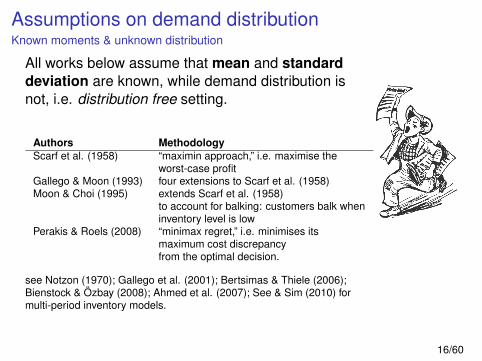
Assumptions on demand distributionKnown moments & unknown distribution

All works below assume that mean and standarddeviation are known, while demand distribution isnot, i.e. distribution free setting.

Authors MethodologyScarf et al. (1958) “maximin approach,” i.e. maximise the

worst-case profitGallego & Moon (1993) four extensions to Scarf et al. (1958)Moon & Choi (1995) extends Scarf et al. (1958)

to account for balking: customers balk wheninventory level is low

Perakis & Roels (2008) “minimax regret,” i.e. minimises itsmaximum cost discrepancyfrom the optimal decision.

see Notzon (1970); Gallego et al. (2001); Bertsimas & Thiele (2006);Bienstock & Özbay (2008); Ahmed et al. (2007); See & Sim (2010) formulti-period inventory models.

16/60

Assumptions on demand distributionUnknown moments & unknown distribution






↑

17/60

Assumptions on demand distributionUnknown moments & unknown distribution

All works below operate without any access to andassumptions on the true demand distributions, i.e.non-parametric setting.

Authors MethodologyHayes, 1971 order statisticsLordahl & Bookbinder, 1994 order statisticsBookbinder & Lordahl, 1989 bootstrappingFricker & Goodhart, 2000 bootstrappingLevi et al. (2007) determine bounds for the number

of samples needed to guaranteean arbitrary approximation ofthe optimal policy

Huh et al. (2009) adaptive inventory policy thatdeal with censored observations

18/60

Assumptions on demand distributionUnknown moments & known distribution






↑

19/60


According to Berk et al. (2007) there are twogeneral approaches for dealing with this setting:the Bayesian and the frequentist.

According to Kevork (2010) another distinction canbe made between approaches assuming thatdemand is fully observed and approachesassuming that demand may be censored.

20/60


Bayesian approaches in the literature:

Fully observed demand Censored demandScarf (1959, 1960) Lariviere & Porteus (1999)Iglehart (1964) Ding & Puterman (1998)Azoury (1985) Berk et al. (2007)Lovejoy (1990) Chen (2010)Bradford & Sugrue (1990) Lu et al. (2008)Hill (1997) Mersereau (2012)Eppen & Iyer (1997)Hill (1999)Lee (2008)Bensoussan et al. (2009)

21/60


Frequentist approaches in the literature:

Authors MethodologyNahmias (1994) stock level is givenAgrawal & Smith (1996) stock level is givenLiyanage & Shanthikumar (2005) “operational statistics:” optimal order quantity

directly estimated from the dataKevork (2010) exploits the sampling distribution of the demand

parameters to study the variability of the estimatesfor the optimal order quantity and associatedexpected total profit.

Akcay et al. (2011) ETOC: expected one-period cost associatedwith operating under an estimated inventorypolicy

Klabjan et al. (2013) integrate distribution fitting androbust optimisation

22/60


Assume now that the demand distribution isknown, but one or more distribution parametersare unknown.

The decision maker has access to a set of M pastrealizations of the demand.

From these she has to estimate the optimal orderquantity (or quantities) and the associated cost.

23/60


Poisson demand, probability mass function:

λ has to be estimated from past realizations.

24/60

A frequentist approachPoint estimates of the parameter(s)

Point estimates of the unknown parameters maybe obtained from the available samples by using:

▶ maximum likelihood estimators, or▶ the method of moments.

Point estimates for the parameters are then usedin place of the unknown demand distributionparameters to compute:

▶ the estimated optimal order quantity Q̂∗, and▶ the associated estimated expected total cost

G(Q̂∗).

25/60

A frequentist approachPoint estimates: example

M observed past demand data d1, . . . , dM.

Demand follows a Poisson distributionPoisson(λ), with demand rate λ.

We estimate λ using the maximum likelihoodestimator (sample mean):

λ̂ =1M

M∑i=1

λi.

The decision maker employs the distributionPoisson(λ̂) in place of the actual unknown demanddistribution.

26/60

A frequentist approachPoint estimates: example

Holding cost: h = 1; penalty cost: p = 3;observed past demand data:{51, 54, 50, 45, 52, 39, 52, 54, 50, 40}.

λ̂ = 48.7, Q̂∗ = 53 and G(Q̂∗) = 9.0035.

time

inventory

0

single period

d = Poisson(λ)

λ = 50

Q* = 55G(Q*) = 9.1222

Q* = 53

G(Q*) = 9.0035

10 observations

27/60

Bayesian approachThe bayesian approach infers the distribution ofparameter λ given some past observations d byapplying Bayes’ theorem as follows

p(λ|d) = p(d|λ)p(λ)∫p(d|λ)p(λ)dλ

where

p(λ) is the prior distribution of λ, and

p(λ|d) is the posterior distribution of λ given theobserved data d.

28/60

Bayesian approachThe prior distribution describes an estimate ofthe likely values that the parameter λ might take,without taking the data into account. It is based onsubjective assessment and/or collateral data.

A number of methods for constructing“non-informative priors” have been proposed(i.e. maximum entropy). These are meant toreflect the fact that the decision maker ignores ofthe prior distribution.

If prior and posterior distributions are in the samefamily, then they are called conjugatedistributions.

29/60

Bayesian approach[Hill, 1997]

Hill [EJOR, 1997] proposes a bayesian approachto the Newsvendor problem.

He considers a number of distributions (Binomial,Poisson and Exponential) and derives posteriordistributions for the demand from a set of givendata.

He adopts uninformative priors to express aninitial state of complete ignorance of the likelyvalues that the parameter might take.

By using the posterior distribution he obtains anestimated optimal order quantity and therespective estimated expected total cost.

30/60

Bayesian approach[Hill, 1997] example

Holding cost: h = 1; penalty cost: p = 3;observed past demand data:{51, 54, 50, 45, 52, 39, 52, 54, 50, 40}.

Q̂∗ = 54 and G(Q̂∗) = 9.4764.

time

inventory

0

single period

d = Poisson(λ)

λ = 50

Q* = 55 G(Q*) = 9.1222Q* = 54

G(Q*) = 9.4764

10 observations

31/60

Drawbacks of existing approachesOnly provide point estimates of the orderquantity and of the expected total cost.

Do not quantify the uncertainty associated withthis estimate.

▶ How do we distinguish a case in which weonly have 10 past observations vs a case with1000 past observations?

The bayesian approach produces results that, forsmall samples, are “biased” by the selection of theprior; further drawbacks are outlined in

J. Neyman. Outline of a theory of statistical estimation based on the classical theory ofprobability. Philosophical Transactions of the Royal Society of London, 236:333—380, 1937

32/60

An alternative approachWe propose a solution method based onconfidence interval analysis [Neyman, 1937].

ObservationSince we operate under partial information, it maynot be possible to uniquely determine “the” optimalorder quantity and the associated exact cost.

We argue that a possible approach consists indetermining a range of “candidate” optimal orderquantities and upper and lower bounds for thecost associated with these quantities.

This range will contain the real optimum accordingto a prescribed confidence probability α.

33/60

An alternative approach

time

inventory

0

single period

d = Poisson(λ)

λ = 50

Q* = 55 G(Q*) = 9.1222

cost = (clb,cub)

confidence = αM observations

candidateorderquantities

34/60

Confidence interval for λConsider a set of M random variates di drawn froma random demand d that is distributed according toa Poisson law with unknown parameter λ.

We construct a confidence interval for theunknown demand rate λ as follows

λlb = min{λ|Pr{Poisson(Mλ) ≥ d̄} ≥ (1 − α)/2},λub = max{λ|Pr{Poisson(Mλ) ≤ d̄} ≥ (1 − α)/2},

where d̄ =∑M

i=0 di.

A closed form expression for this interval hasbeen proposed by Garwood [1936] based on thechi-square distribution.

35/60

Confidence interval for λ: exampleConsider the set of 10 random variates

{51, 54, 50, 45, 52, 39, 52, 54, 50, 40},

and α = 0.9.

The confidence interval for the unknown demandrate λ is

(λlb, λub) = (45.1279, 52.4896),

Note that, by chance, this interval covers the actualdemand rate λ = 50 used to generate the sample.

36/60

Candidate order quantitiesLet Q∗

lb be the optimal order quantity for theNewsvendor problem under a Poisson(λlb) demand.

Let Q∗ub be the optimal order quantity for the

Newsvendor problem under a Poisson(λub)demand.

Since ∆G(Q) is non-decreasing in Q, accordingto the available information, with confidenceprobability α, the optimal order quantity Q∗ is amember of the set {Q∗

lb, . . . ,Q∗ub}.

37/60

Candidate order quantities

λ0

0.5

1

Pr{Poisson(λ) ≤ Q∗lb} Pr{Poisson(λ) ≤ Q∗

ub}

Pr{Poisson(λ) ≤ Q∗}

λ̄

λlb λub

β

increasing Q

38/60

Candidate order quantities: exampleConsider the set of 10 random variates

{51, 54, 50, 45, 52, 39, 52, 54, 50, 40},

and α = 0.9.

The candidate order quantities are

time

inventory

0

single period

d = Poisson(λ)

λ = 50

Q* = 55 G(Q*) = 9.1222

cost = (clb,cub)

candidateorderquantities


50

57

39/60

Confidence interval for the expected total costFor a given order quantity Q we can prove that

GQ(λ) = h∑Q

i=0 Pr{Poisson(λ) = i}(Q − i)+p∑∞

i=Q Pr{Poisson(λ) = i}(i − Q),

is convex in λ.

Upper (cub) and lower (clb) bounds for the costassociated with a solution that sets the orderquantity to a value in the set {Q∗

lb, . . . ,Q∗ub} can be

easily obtained by using convex optimizationapproaches to find the λ∗ that maximizes orminimizes this function over (λlb, λub).

40/60

Confidence interval for the expected total cost

expecte

d tota

l cost: G

Q(λ

)

λlb λub

cub

clb

λ*

for Q ∈ {Q∗lb, . . . ,Q∗

ub}.

41/60


p0

GpQ(λ)Gh

Q(λ)GQ(λ)

λ̄

λlb λub

λ∗Q,maxλ∗

Q,min

GQ(λ̄)

cub

clb

A

42/60


p0

GpQ(λ)Gh

Q(λ)GQ(λ)

λ̄

λlb λub

GQ(λ̄)

cub

clb

B

43/60


q0

GpQ(λ)Gh

Q(λ)GQ(λ)

λ̄

GQ(λ̄)

λlb λub

cub

clb

C

44/60


q

GpQ(λ)Gh

Q(λ)GQ(λ)

λ̄

GQ(λ̄)

λlb λub

cpub

cplb

D

45/60

Expected total cost: exampleConsider the set of 10 random variates

{51, 54, 50, 45, 52, 39, 52, 54, 50, 40},

and α = 0.9.

The upper and lower bound for the expected totalcost are

time

inventory

0

single period

d = Poisson(λ)

λ = 50

Q* = 55 G(Q*) = 9.1222

cost = (8.6,14.6)

candidatequantities


50

57

46/60

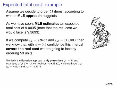
Expected total cost: exampleAssume we decide to order 53 items, according towhat a MLE approach suggests.

As we have seen, MLE estimates an expectedtotal cost of 9.0035 (note that the real cost wewould face is 9.3693).

If we compute clb = 8.9463 and cub = 11.0800, thenwe know that with α = 0.9 confidence this intervalcovers the real cost we are going to face byordering 53 units.

Similarly, the Bayesian approach only prescribes Q̂∗ = 54 andestimates G(Q̂∗) = 9.4764 (real cost is 9.1530), while we know thatclb = 9.0334 and cub = 10.3374.

47/60

Lost salesConsider the case in which unobserved lost sales occurredand the M observed past demand data, d1, . . . , dM, only reflectthe number of customers that purchased an item when theinventory was positive.

The analysis discussed above can still be applied providedthat the confidence interval for the unknown parameter λ of thePoisson(λ) demand is computed as

λlb = min{λ|Pr{Poisson(M̂λ) ≥ d̄} ≥ (1 − α)/2},λub = max{λ|Pr{Poisson(M̂λ) ≤ d̄} ≥ (1 − α)/2}.

where M̂ =∑M

j=1 Tj, and Tj ∈ (0, 1) denotes the fraction oftime in day j — for which a demand sample dj is available —during which the inventory was positive.

48/60

Binomial demandN customer enter the shop on a given day, theunknown purchase probability of the Binomialdemand is q ∈ (0, 1).

The analysis is similar to that developed for aPoisson demand.

Also in this case we prove that GQ(q) is convex inq.

Lost sales can be easily incorporated in theanalysis.

49/60

Exponential demandThe interval of candidate order quantities can beeasily identified.

The analysis on the expected total cost iscomplicated by the fact that GQ(λ) is not convex.

Extension to include lost sales is difficult.

50/60

Exponential demandA number of properties of GQ(λ) can beexploited to find upper and lower bounds for theexpected total cost.

0λ

hQ

GpQ(λ)Gh

Q(λ)GQ(λ)

51/60

Exponential demandA number of properties of GQ(λ) can beexploited to find upper and lower bounds for theexpected total cost.

λ

Q

GQ(λ)

GQ∗lb(λub)

GQ∗ub(λub)

GQ∗lb(λlb)

52/60

Experiment setup

Parameter Valuesh 1p 2, 4, 8, 16M 5, 10, 20, 40, 80α 0.9N 1, 2, 4, 8, 16, 32, 64p 0.5, 0.75, 0.95λ 0.125, 0.25, 0.5, 1, 2, 4, 8, 16, 32, 64

53/60

Comparison with MLE and Bayesian approaches

0.01

0.10

1.00

100.00

Samples

MAPE

5 10 20 40 80

MLE

0.01

0.10

1.00

100.00

Samples

MAPE

5 10 20 40 80

Bayes

Estimated cost Actual cost

0.01

0.10

1.00

10.00

Samples

MAPE

5 10 20 40 80

0.01

0.10

1.00

10.00

Samples

MAPE

5 10 20 40 80

bin

om

ial

MLE Bayes0.01

0.10

1.00

100.00

Samples

MAPE

5 10 20 40 80

0.01

0.10

1.00

100.00

Samples

MAPE

5 10 20 40 80

0.01

0.10

1.00

100.00

Samples

MAPE

5 10 20 40 80

0.01

0.10

1.00

100.00

Samples

MAPE

5 10 20 40 80

MLE Bayes MLE Bayes

Po

isso

n

0.01

0.10

1.00

100.00

Samples

MAPE

5 10 20 40 80

0.01

0.10

1.00

100.00

Samples

MAPE

5 10 20 40 80

0.01

0.10

1.00

100.00

Samples

MAPE

5 10 20 40 80

0.01

0.10

1.00

100.00

Samples

MAPE

5 10 20 40 80

MLE Bayes MLE Bayes

exp

on

en

tia

l

54/60

Confidence-based optimisation resultsb

ino

mia

lP

ois

son

exp

on

en

tia

l

Exact Approximate0

.88

0.9

00

.92

0.9

4

Samples

5 10 20 40 80

Samples

5 10 20 40 80

0.2

0.5

12

Samples

5 10 20 40 80

(Q*

- Q

* )/

Q*

ub

lb

Exact

Samples

5 10 20 40 80

Approximate

(c*

- c

* )/

G(Q

*)u

blb

0.2

0.5

12

51

0

Samples

5 10 20 40 80

Exact

Samples

5 10 20 40 80

Approximate

0.2

0.5

12

51

0

Samples

5 10 20 40 80

Exact

Samples

5 10 20 40 80

Approximate

(c

-

c

)/

G(Q

*)u

blb

ML

EM

LE

Co

ve

rag

e p

rob

ab

ilit

yC

ov

era

ge

pro

ba

bil

ity

0.7

50

.80

0.8

50

.90

0.9

51

.00

Samples

5 10 20 40 80

Samples

5 10 20 40 80

0.8

Samples

5 10 20 40 80

(Q*

- Q

* )/

Q*

ub

lb

0.6

0.4

0.2

0

Samples

5 10 20 40 80

(c*

- c

* )/

G(Q

*)u

blb

Samples

5 10 20 40 80

(c

-

c

)/

G(Q

*)u

blb

ML

EM

LE

0.0

50

.10

.20

.51

25

10

Samples

5 10 20 40 80

Samples

5 10 20 40 80

0.0

50

.10

.20

.51

25

10

Samples

5 10 20 40 80

Co

ve

rag

e p

rob

ab

ilit

y

Samples

5 10 20 40 80

0.7

50

.80

0.8

50

.90

0.9

51

.00

Samples

5 10 20 40 80

2.5

Samples

5 10 20 40 80

(Q*

- Q

* )/

Q*

ub

lb

00

.51

1.5

2

Samples

5 10 20 40 80

(c*

- c

* )/

G(Q

*)u

blb

0.0

50

.10

.20

.51

52

10

Samples

5 10 20 40 80

Samples

5 10 20 40 80

(c

-

c

)/

G(Q

*)u

blb

ML

EM

LE

Samples

5 10 20 40 80

0.0

50

.10

.20

.51

52

10

Samples

5 10 20 40 80

Coverage probability Order quantity Optimal cost MLE cost

55/60

DiscussionWe presented a confidence-based optimizationstrategy to the Newsboy problem with unknowndemand distribution parameter(s).

We applied our approach to three maximumentropy probability distributions of theexponential family.

We showed the advantages of our approachover two existing strategies in the literature.

For two demand distributions we extended theanalysis to include lost sales.

56/60

Published articles: EJOR 2014

57/60

Published articles: AIJ 2015

58/60

Future worksConsider other probability distributions (e.g.Normal, LogNormal, Multinomial etc.).

Further develop the analysis on lost sales forthe Exponential distribution.

Extend the methodology to a non-parametricsetting.

Apply confidence-based optimization to otherstochastic optimization problems.

59/60

Questions

60/60

Date post:	16-May-2020
Category:	Documents
Upload:	others
View:	5 times
Download:	0 times

Confidence-based optimization for the Newsvendor problem · Conﬁdence-based optimization for the...

Documents