Conformal Field Theory Lecture Notes

Conformal Field Theory Lecture Notes

Perpetually in progress

Dimitris Manolopoulos* and Konstantinos Sfetsos

November 20, 2020

National Centre for Scientific Research“Demokritos”

Institute of Nuclear and Particle Physics

Department of Nuclear & Particle PhysicsFaculty of Physics

National and Kapodistrian University of Athens

Abstract

Lecture notes prepared for the master level students at the department of Physicsof the National and Kapodistrian University of Athens. In particular an introductionis given to those areas of CFT that are most relevant for those interested to take afist course in the subject with a direction for string theory applications. These lecturenotes are perpetually in progress and they will be updated with new material as wemay see fit.

*Email: [email protected]: [email protected]

http://happen.inp.demokritos.gr/

http://users.uoa.gr/~ksfetsos/

Contents

Introduction 3

1 Conformal Invariance 61.1 Symmetry in Physics . . . . . . . . . . . . . . . . . . . . . . . . . . . . . . . . . . . . . . . . . 61.2 The Conformal Group in d Dimensions . . . . . . . . . . . . . . . . . . . . . . . . . . . . . . 8

1.2.1 Representations of the Conformal Group . . . . . . . . . . . . . . . . . . . . . . . . . . 111.3 Conformal Invariance in 2 Dimensions . . . . . . . . . . . . . . . . . . . . . . . . . . . . . . . 13

2 Correlation Functions 152.1 The Energy-Momentum Tensor . . . . . . . . . . . . . . . . . . . . . . . . . . . . . . . . . . . 172.2 Ward Identities . . . . . . . . . . . . . . . . . . . . . . . . . . . . . . . . . . . . . . . . . . . . 18

2.2.1 Holomorphic form of the Ward Identities . . . . . . . . . . . . . . . . . . . . . . . . . 212.3 Operator Product Expansion . . . . . . . . . . . . . . . . . . . . . . . . . . . . . . . . . . . . 23

2.3.1 The Free Boson . . . . . . . . . . . . . . . . . . . . . . . . . . . . . . . . . . . . . . . . 242.3.2 The Free Fermion . . . . . . . . . . . . . . . . . . . . . . . . . . . . . . . . . . . . . . 26

3 The Operator Formalism 283.1 The Virasoro Algebra . . . . . . . . . . . . . . . . . . . . . . . . . . . . . . . . . . . . . . . . 293.2 Highest Weight Representations . . . . . . . . . . . . . . . . . . . . . . . . . . . . . . . . . . . 313.3 The Free Boson . . . . . . . . . . . . . . . . . . . . . . . . . . . . . . . . . . . . . . . . . . . . 353.4 Vertex Operators . . . . . . . . . . . . . . . . . . . . . . . . . . . . . . . . . . . . . . . . . . . 37

4 CFT on the Torus 404.1 Modular Invariance . . . . . . . . . . . . . . . . . . . . . . . . . . . . . . . . . . . . . . . . . . 434.2 The Free Boson on the Torus . . . . . . . . . . . . . . . . . . . . . . . . . . . . . . . . . . . . 454.3 Compactified Boson and T -Duality . . . . . . . . . . . . . . . . . . . . . . . . . . . . . . . . . 464.4 Fusion Algebra and Verlinde’s Formula . . . . . . . . . . . . . . . . . . . . . . . . . . . . . . . 474.5 Rational Conformal Field Theory . . . . . . . . . . . . . . . . . . . . . . . . . . . . . . . . . . 48

A Normal ordering 50A.1 Wick’s Theorem . . . . . . . . . . . . . . . . . . . . . . . . . . . . . . . . . . . . . . . . . . . 50

B Generalized normal ordering 52B.1 Generalized Wick’s Theorem . . . . . . . . . . . . . . . . . . . . . . . . . . . . . . . . . . . . 53

INRODUCTION

Introduction

Conformal symmetry is a potent tool in the construction of two-dimensional conformal quan-tum field theories which are very special in the following sense. The symmetry group oftransformations which leaves angles invariant in Minkowski space is the conformal group.While in d dimensions the conformal group is isomorphic to the Poincare group in d + 2dimensions and thus it is finite dimensional, in two dimensions there is an infinite variety ofconformal transformations and thus the symmetry algebra corresponding to these conformaltransformations is infinite dimensional. This is a very powerful tool since this high degree ofsymmetry imposes many natural constraints so that any QFT in two dimensions with con-formal symmetry has a structure that makes it clearly arranged. There are many examples ofsuch theories which are completely solvable in the sense that one can compute accurately inprinciple all the correlation functions, from which observable quantities are obtained in fieldtheories. Making some times such exact statements in nontrivial situation without relyingon the mysteries of perturbation theory is at least a very satisfying and interesting result.

However, one might say that although all this is true, two dimensions are not quiteenough to describe what seems to be the real world in four space-time dimensions and thisis a fair argument. This raises the question whether or not two-dimensional conformal fieldtheories are significant, if not at all important, as a language in physics and if their structurecan capture, describe and substantiate measurable processes. The answer to this question isthreefold, at least to our knowledge.

Firstly, in statistical and condensed matter physics there are many models and theorieswhich take place in two dimensions and thus two-dimensional conformal field theories playand essential role. For example, one might be interesting in phenomena which are confinedon the two-dimensional boundary of a three-dimensional object, or a system with one spatialdimension which evolves in time whose history is thus a two-dimensional surface. If thesesituations are accompanied by ceratin symmetries, the most important of which is scaleinvariance, then two-dimensional conformal field theory can be utilized. The critical Isingmodel whose continuum limit is described by a two-dimensional conformal field theory ofcentral charge c = 1/2, is probably a famous example of such a situation.

Furthermore, two-dimensional conformal field theory is intimately connected, in a senseeven identical with perturbative string theory. String theory is the most famous candidatefor a grand unified theory that describes all known physical interactions. That is, electro-magnetism, gravity as well as the weak and strong interactions, all in a unified manner. Theunderlying formulation of string theory is described by an action principle, where the actionis an integral over the two-dimensional surface swept out by the superstring as it propagatesin space and time. This action is invariant under conformal transformations of the world-sheet coordinates and Weyl transformations of the worldsheet metric, which implements theconformal symmetry.

Last but not least, two-dimensional conformal field theory serves as an interface betweenphysics and mathematics. This might seem tautological in the sense that most of physics isformulated in some kind of mathematical language, but the above statement is meant in thestronger sense that both mathematicians and physicists pursue common research with openmind for the views and ideas of the other side. While in most other QFTs the mathematicians

D. ManolopoulosNCSR ”Demokritos”

3 K. SfetsosUniversity of Athens

INRODUCTION

some times cannot make sense of the concepts employed by physicists, in a two-dimensionalconformal field theory this goal is much closer to be achieved. For example, in d-dimensionalQFTs one usually assumes a path integral description of the theory, however the path integralis not a well defined mathematical object. In other words, the path integral approach hasthe disadvantage of not being defined rigorously, because it is unclear what measure onemay put on the infinite dimensional space the path integral is over. In a two-dimensionalconformal field theory, a path integral description is not explicitly needed, although one canalways implicitly assume one. String theory was also the motivation for Segal to give hisabstract definition of conformal field theory. His work has been highly influential for manymathematicians working on conformal field theory but we will not go any further into thismatter. The point here is that mathematicians on one hand can be inspired by the intuitionand insight of physicists and use this as a motivation in order to develop new structures orgain better understanding of known ones. Physicists on the other hand can appreciate anduse these deeper mathematical structures in order to uncover the fundamental structure ofa physical system, otherwise it should not be spoken of true understanding.

In these lecture notes a short introduction to Conformal Field Theory (CFT) is presented.It should be noted however, that it is beyond the scope of these notes to present a full sum-mary of CFT. Conformal field theory is a highly developed subject with many connectionsto different areas of physics and mathematics as well as with many excellent reviews andtextbooks available. A selection recommended by the authors, in alphabetical order is

i Recommended literature on 2-dimensional CFT

[ASG89] An introduction by Alvarez-Gaume, Sierra and Gomez, written with an emphasison the connection to knots and quantum groups.

[BPZ] The original paper by Belavin, Polyakov and Zamolodchikov.

[BYB] The book by Di Francesco, Mathieu and Senechal, which develops CFT from firstprinciples. The treatment is self-contained, pedagogical, exhaustive and includesbackground material on QFT, statistical mechanics, Lie and affine Lie algebras,WZW models, the coset construction e.t.c.

[Ca08] Lectures given at Les Houches (2008) by John Cardy with emphasis to statisticalmechanics.

[Gab99] An overview of CFT centered on the role of the symmetry generating chiral algebraby Matthias Gaberdiel.

[Gin] Lectures given at Les Houches (1988) by Paul Ginsparg.

[Se02] The axiomatic formulation of CFT by Segal in the language of category theoryand modular functors.

In the following, an introduction is given to those areas of CFT that are most relevantfor those interested to take a fist course in the subject with a direction for string theoryapplications. In a few cases the results might just be stated since they are considered asstandard in the literature and the readers may refer themselves to the recommendationsmentioned above or to citations within the main text, for further details.



INRODUCTION

b Exercise 0.1. We certainly did not manage to remove all the errors from these notes.The first exercise is to find all the errors and send them to us.



1 CONFORMAL INVARIANCE

1 Conformal Invariance

1.1 Symmetry in Physics

This subsection is somewhat of general interest since we will explain in some detail what doesone mean by a symmetry in physics. The ideas developed here will be used later on whenwe will discuss the consequence of an infinitesimal continuous symmetry transformation onthe correlation functions of the theory and the Ward identities.

Symmetries are an important concept in physics. Recent theories are almost entirelyconstructed from symmetry considerations alone. Some notable examples are gauge theories,supergravity theories and two-dimensional conformal field theories. In this approach onedemands the existence of a certain symmetry and wonders what theories with this propertyone can construct.

Recall for example, in quantum mechanics the states of a quantum system are elementsof the Hilbert space H. Given a state ψ(0) ∈ H at time zero, its time evolution is describedby a self-adjoint operator H, the Hamiltonian on H. Thus, at time t the system will be inthe state

ψ(t) = eti~Hψ(0). (1.1)

In general, given a self adjoint operator A ∈ H, such that [A,H] = 0, one can consider a oneparameter family of operators UA(s) = eisA, for s ∈ R. The operators UA(s) are unitary sothey preserve probabilities and commute with time-evolution:

ψ eti~Hψ

UA(s)ψ UA(s)eti~Hψ = e

ti~HUA(s)ψ

//evolve

//evolve

UA(s)

UA(s) (1.2)

In a QFT on the other hand, the symmetries will act on the fields of the theory. Thesefields are scalar fields, vector fields and spinor fields. In these notes we will mostly beconcerned with scalar fields φ. A local field φ(x) ≡ φ(x, t) arises from giving the time-zerofield φ(~x), time dependence generated by a local Hamiltonian H,

φ(x) = U †H(t)φ(~x)UH(t), (1.3)

where UH(t) = e−itH , (in units where ~ = 1) is the time evolution operator. Then, asymmetry is an invertible map f on the space of fields (or space of states) which commuteswith the time evolution map ρ, where ρ is known as a projective representation and it actson the time-zero fields as in (1.3) i.e. φ 7→ U †φU :

φ φ(x)

φ′ φ′(x)

//ρ

//ρ

f

f (1.4)

In words, what the above commutative diagram says is the following. If one started from φand evolved in time with ρ to arrive to φ(x) and then performed a symmetry transformation



1.1 Symmetry in Physics 1 CONFORMAL INVARIANCE

f , to finally arrive to φ′(x) = f(φ(x)), it would have been the same as if one started from φand first performed the symmetry transformation f , followed by ρ. That is f ρ = ρ f .

Z

Example 1.1. Lets take f to be the map Uθ(q) : θ 7→ eiqθ ∈ U(1) for q ∈ R. Then (1.4) simplysays that

Uθ(q)(UH(t)†φ(~x)UH(t)

)= φ′(x) = UH(t)† (Uθ(q)φ(~x))UH(t). (1.5)

This equality holds because θ and H commute. This example is a U(1) symmetry, one can gaugesuch a symmetry if one supposes that the parameter θ is allowed to be a function of space-time:θ(x). We see that the map Uθ(q) provides a representation of U(1). One can now try to generalizethis by replacing U(1) by any Lie group G and taking the fields to take values in a space that carriesa representation R(g) of G, for some group element g ∈ G. The group G is usually called the gaugegroup and this generalization is known as a Yang-Mills theory.

Consider now the family of operators UT (ε) = eiεaTa. From the commutative diagram

(1.4) we see that in order for this to be a symmetry, (i.e. so that one must be able to writean equality of the form (1.5)) the operators T a have to commute with H. If the parametersεa are very small then we take the infinitesimal symmetry transformation

UT (ε) = 1 + iεaTa +O

(ε2). (1.6)

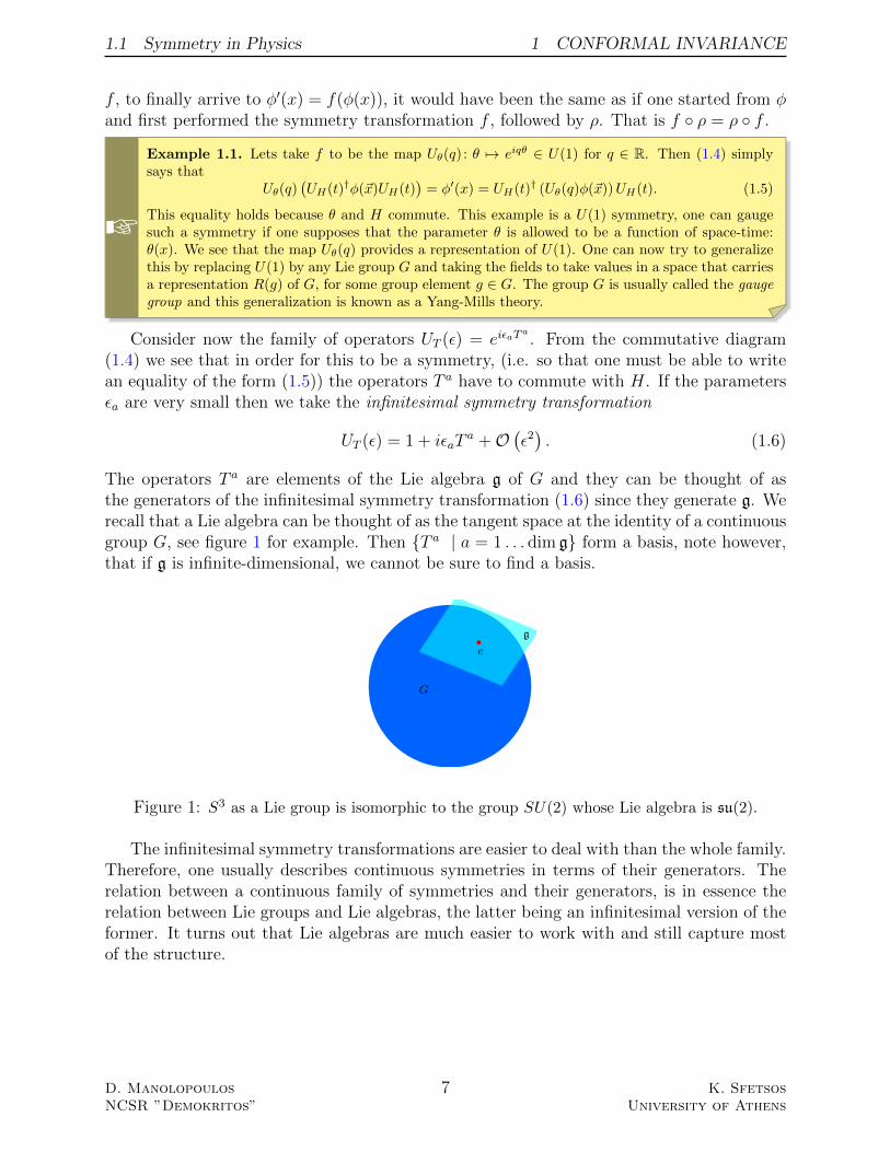
The operators T a are elements of the Lie algebra g of G and they can be thought of asthe generators of the infinitesimal symmetry transformation (1.6) since they generate g. Werecall that a Lie algebra can be thought of as the tangent space at the identity of a continuousgroup G, see figure 1 for example. Then T a | a = 1 . . . dim g form a basis, note however,that if g is infinite-dimensional, we cannot be sure to find a basis.

g

e

G

Figure 1: S3 as a Lie group is isomorphic to the group SU(2) whose Lie algebra is su(2).

The infinitesimal symmetry transformations are easier to deal with than the whole family.Therefore, one usually describes continuous symmetries in terms of their generators. Therelation between a continuous family of symmetries and their generators, is in essence therelation between Lie groups and Lie algebras, the latter being an infinitesimal version of theformer. It turns out that Lie algebras are much easier to work with and still capture mostof the structure.



1.2 The Conformal Group in d Dimensions 1 CONFORMAL INVARIANCE

1.2 The Conformal Group in d Dimensions

In this and the following subsection we will talk about some aspects of CFT in d dimensions.The rest of the notes will concentrate in two dimensional CFT which we will develop inmore detail. Consider a flat metric gµν on a space-time manifold M . We say that thetransformation xµ 7→ x′µ is a conformal transformation of the coordinates if it leaves themetric tensor invariant

gµν(x) 7→ g′µν(x′) = Ω2(x)gµν(x), (1.7)

up to a scale factor Ω2(x), called the conformal factor. This means that the physics of thetheory under consideration looks the same at all length scales. In other words, conformalfield theories preserve angles but not necessarily lengths.

Z

Example 1.2. Consider the Minkowski metric in two dimensions in light cone coordinates σ± = x±t

ds2 = dσ+dσ−.

Using the conformal transformation σ± = tanσ′±, with σ′± ∈ (−π/2, π/2) one obtains

ds′2 = cos2 σ+ cos2 σ−ds2 = dσ′+dσ

′−,

from which we immediately see that Ω2 = cos2 σ+ cos2 σ−.

b

Exercise 1.3. Start with the flat space metric in R1,d−1 in polar coordinates

ds2R1,d−1 = −dt2 + dr2 + r2dS2

d−2,

where dS2d−2 is the metric on Sd−2. Consider now the coordinate transformation

t = Rsinh

(τR

)coshu+ cosh

(τR

) , r = Rsinhu

coshu+ cosh(τR

) ,where R is the constant radius of Sd−2. Find the conformally transformed metric and show thatthe conformal factor is given by

Ω2 =1(

coshu+ cosh(τR

))2 .Identify the topology of the conformally transformed metric. What does R now represents in thisnew metric?

The set of all conformal transformations in d dimensions forms a group, the conformalgroup, which is isomorphic to the group of Poincare transformations SO(d + 1, 1) in d + 2dimensions (we will see this isomorphism in a moment), with 1

2(d+ 1)(d+ 2) parameters and

thus it is finite dimensional. For an infinitesimal transformation xµ 7→ x′µ = xµ + εµ(x) tobe conformal the metric tensor, at first order in ε changes as follows

δgµν = (Ω2 − 1)gµν = 2∂(µεν). (1.8)

bExercise 1.4. Convince yourself that under the infinitesimal transformation the metric tensorindeed changes as stated in (1.8). Hint: use the transformation rule for the metric up to first orderin ε.




The conformal factor is determined by taking traces

Ω2 = 1 +2

d∂µε

µ. (1.9)

Combining equations (1.8) and (1.9) we get

∂(µεν) =1

d∂ρε

ρgµν . (1.10)

The last equation implies that (gµν∂

2 + (d− 2)∂µ∂ν)

Ω2 = 0, (1.11)

which after contracting with gµν reduces to

(d− 1)∂2Ω2 = 0. (1.12)

bExercise 1.5. Derive equation (1.11) from (1.10). Hint: Apply an extra derivative ∂ρ on (1.10) andpermute indices. Then take a linear combination to arrive at 2∂µ∂νερ = (gνρ∂µ+ gµρ∂ν − gµν∂ρ)Ω2.Finally, contract with gµν and apply ∂ν to arrive to (1.11).

Clearly, the case d = 1 is trivial and it simply means that everything is conformal in onedimension since there are no angles. The case d = 2 will be treated in more detail later on.Now, for d > 2 we see that ε is at most quadratic in x, so we have the following possibilities:

For ε zeroth order in x: translations εµ = aµ.

For ε linear in x we have two possibilities:

1. scale transformations εµ = λxµ

2. rotations εµ = ωµνxν , (ω(µν) = 0)

For ε quadratic in x: special conformal transformations or briefly SCTs

εµ = bµx2 − 2xµb · x.

Manifestly, the SCTs are nothing but an inversion plus a translation, x′µ

x′2= xµ

x2 + bµ.

More abstractly, with think of the infinitesimal transformations as being generated bythe linear operators

Pµ = −i∂µMµν = 2ix[µ∂ν]

D = −ixµ∂µKµ = −i(2xµxν∂ν − x2∂µ)

. (1.13)

The factors of i are chosen to ensure that the generators are Hermitian. These generatorscan then also be though of as applying on different objects, e.g. space-time fields rather




than space-time points. In other words we have an abstract algebra and its action on xµ ismerely one representation.

These linear operators generate the conformal algebra, which is locally isomorphic toSO(p + 1, q + 1). To see this a little counting will help. If we set p + q = d then we seethat there are p+ q generators for Pµ (translations), 1

2(p+ q)(p+ q− 1) for Mµν (rotations),

1 for D (dilations) and finally p + q for Kµ (SCTs). In total, the conformal algebra has12(p+ q + 1)(p+ q + 2) generators. The conformal algebra is defined by the commutators

[D,Pµ] = −iPµ[D,Kµ] = −iKµ

[Kµ, Pν ] = 2i(ηµνD −Mµν)

[Kρ,Mµν ] = i(ηρµKν − ηρνKµ)

[Pρ,Mµν ] = i(ηρµPν − ηρνPµ)

[Mµν ,Mρσ] = i(ηνρMµσ + ηµσMνρ − ηµρMνσ − ηνσMµρ)

. (1.14)

b Exercise 1.6. Show this using (1.13).

Redefining now

Jµν = Mµν

J−1,µ =1

2(Pµ −Kµ)

J−1,0 = D

J0,µ =1

2(Pµ +Kµ)

, (1.15)

with Jab = −Jba, and a, b ∈ −1, 0, 1, . . . , d, we see that the new generators satisfy theSO(d+ 1, 1) commutation relations

[Jab, Jcd] = i(ηadJbc + ηbcJad − ηacJbd − ηbdJac), (1.16)

which shows the isomorphism between the conformal group in d dimensions and SO(d+1, 1)in d+ 2 dimensions as mentioned above.

One can integrate to finite conformal transformations. Translations and rotations formthe Poincare group

x′µ = xµ + aµ

x′µ = Λµνx

ν , (Λµν ∈ SO(p, q))

(Ω2 = 1). (1.17)

Next for the dilations we have

x′µ = λxµ, (Ω2 = λ−2), (1.18)

while for the SCT’s

x′µ =bx2 + x

b2x2 + 2bx+ 1, (Ω2 = (b2x2 + 2bx+ 1)2). (1.19)




1.2.1 Representations of the Conformal Group

The linear operators in (1.13) are not the full generators of the conformal symmetry sinceby the discussion in subsection 1.1 they must include the continuous symmetry generatorsT a, which form a representation of the conformal group. Under an infinitesimal symmetrytransformation the fields transform as

φ(x)→ φ′(x) = φ(x) + δεφ(x) = (1− iεaT a)φ(x). (1.20)

where δε ≡ δδεa

, expresses the variation of the field with respect to the infinitesimal parameterεa. Therefore, one must add T a to the space-time part of (1.13) in order to obtain the fullsymmetry. To proceed, it is customary to rewrite (1.20) as

δεφ(x) ≡ φ′(x)− φ(x) = −iεaT aφ(x), (1.21)

Furthermore, the coordinates under a general infinitesimal transformation change as

xµ → x′µ = xµ + εa(x)δεxµ. (1.22)

Under this change of coordinates the various fields change also as

φa(x)→ φ′a(x′) = Xa[φ(x)]. (1.23)

This means that, the field considered as a mapping φ : Rd → M, from space-time to sometarget spaceM is affected in two ways, first by the functional change φ′ = X[φ] and secondby the change of argument x→ x′. Expanding to first order in εa we have

φ′(x′)(1)= φ(x) + εa(x)Xa[φ(x)]

(2)= φ(x′µ − εaδεx′µ) + εaXa[φ(x′)]

(3)= φ(x′)− εaδεx′µ∂′µφ(x′) + εaXa[φ(x′)]

, (1.24)

where in step (1) we wrote (1.23) in infinitesimal form, in step (2) we did an inverse trans-formation of the coordinates x = x′ − εa(x)δεx

′µ and finally in step (3) we did an expansionto first order in εa. From (1.24) it can also be seen that

εaXa[φ(x)] = φ′(x′)− φ(x). (1.25)

We can treat x′ as a dummy variable in (1.24) to finally take

δεφ(x) = −εaδεxµ∂µφ(x) + εaXa[φ(x)] = −iεaTaφ(x). (1.26)

Therefore, the explicit expression for the generator is

Taφ(x) = i (Xa[φ(x)]− δεxµ∂µφ(x)) . (1.27)

For an infinitesimal translation generated by εµ = aµ we see that x′µ = xµ + aµ andtherefore, φ′(x′) = φ′(x+ a) = φ(x), thus Xa[φ] = 0. So we conclude that

Pµ = −i∂µ. (1.28)




For an infinitesimal Lorentz transformation εµ = ωµνxν

x′µ = Λµνx

ν , Λµν = δµν + ωµν , (ωµν 1). (1.29)

Plugging this into the condition

ηµν = ΛµρΛ

νση

ρσ =⇒ ω(µν) = 0. (1.30)

b Exercise 1.7. Show this by keeping ω to first order.

One can use this to write (1.29) as

x′µ = xµ + ω[νσ]ηµ[ν xσ], (1.31)

which impliesδωx

µ = ηµ[ν xσ]. (1.32)

Under the infinitesimal Lorentz transformations (1.29) the field φ(x) will transform as

φ′(x′) = φ(Λµνx

ν) = U(Λ)φ(x), (1.33)

where U(Λ), is a matrix representation of the Lorentz group depending on Λ and to firstorder in ω, is given by

U(Λ) = 1− i

2ωµνS

µν , (1.34)

where the factor of 1/2 compensates for the double counting of transformation parameterscaused by the full contraction of indices and Sµν is some Hermitian matrix obeying theLorentz algebra. Thus, we see that Xa[φ] = − i

2Sµνφ(x). Finally, using (1.27) the full

generator Mµν , of infinitesimal Lorentz transformations can be written as

i

2Mµνφ(x) =

(x[µ∂ ν] − i

2Sµν)φ(x), (1.35)

from which we immediately see that

Mµν = 2ix[µ∂ν] + Sµν . (1.36)

b

Exercise 1.8. Show that for an infinitesimal dilation x′µ = (1 + λ)xµ, for which

φ′(x′) = (1− λ∆)φ(x), (λ 1), (1.37)

with ∆ the generator of dilations, the corresponding symmetry generator is given by

D = −i (xµ∂µ + ∆) . (1.38)

We will use these later on to derive the Ward identities that correspond to each one ofthese generators.



1.3 Conformal Invariance in 2 Dimensions 1 CONFORMAL INVARIANCE

1.3 Conformal Invariance in 2 Dimensions

In two dimensions there exists an infinite variety of coordinate transformations that, althoughnot everywhere well defined, are locally conformal and they are holomorphic mappings fromthe complex plane to itself. The local conformal symmetry is of special importance intwo dimensions since the corresponding symmetry algebra is infinite-dimensional. Thesestatements will become more clear in a moment.

Note that for d = 2 and gµν = δµν , equations (1.10) are just the Cauchy-Riemannequations

∂1ε1 = ∂2ε2 and ∂1ε2 = −∂2ε1. (1.39)

These equations are the conditions for a function to be conformal. If we identify the twodimensional Euclidean space with the complex plane we may write

ε(z) = ε1 + iε2, ε(z) = ε1 + iε2, (1.40)

in the complex coordinates z = x + iy and z = x − iy. If we denote the metric tensor incomplex coordinates as gαβ, where the indices α, β take the values z and z in that order andwe set

∂ ≡ ∂z and ∂ ≡ ∂z, (1.41)

then the following table summarizes the relation between some quantities in Cartesian andcomplex coordinates.

Quantity Cartesian coordinates (x, y) Complex coordinates (z, z)

xµ x = 12(z + z), y = − i

2(z − z) z = x+ iy, z = x− iy

∂µ ∂x = ∂ + ∂, ∂y = i(∂ − ∂) ∂ = 12(∂x − i∂y), ∂ = 1

2(∂x + i∂y)

gµν gµν = gµν =

(1 00 1

)gαβ =

(0 1

212

0

), gαβ =

(0 22 0

)Table 1: Relation between some quantities in Cartesian and complex coordinates

b Exercise 1.9. Show the relations in table 1.

In this language, the holomorphic Cauchy-Riemann equations become

∂w(z, z) = 0, (1.42)

whose solution is any holomorphic mapping z 7→ w(z) = z + ε(z). Analytic functionsautomatically preserve angles and we see that there are infinitely many independent suchtransformations.

b Exercise 1.10. Show the holomorphic Cauchy-Riemann equations (1.42) from (1.39) using table1.

Everything we have said up to now is purely local, we have not yet imposed any conditionsfor the conformal transformations to be everywhere well defined and invertible. Strictly



1.3 Conformal Invariance in 2 Dimensions 1 CONFORMAL INVARIANCE

speaking, in order to form a group, the mappings must be invertible and must map thewhole plane to itself (more precisely the Riemann sphere C ∪ ∞). One, therefore, mustdistinguish global conformal transformations, which satisfy these requirements, from thelocal ones, which are not everywhere well defined. In order to proceed and find these globalconformal transformations we need to find first the commutator relations for the infinitedimensional local conformal algebra and then mod out the non invertible transformations.We start by taking the basis

z 7→ w(z) = z + εn(z), z 7→ w(z) = z + εn(z), n ∈ Z, (1.43)

where, εn(z) is a polynomial in z of degree n+ 1

εn(z) = −zn+1, εn(z) = −zn+1. (1.44)

The corresponding infinitesimal generators are

`n = −zn+1∂, ¯n = −zn+1∂. (1.45)

These satisfy the algebra

[`m, `n] = (m− n)`m+n, [¯m, ¯n] = (m− n)¯

m+n, [`m, ¯n] = 0. (1.46)

b Exercise 1.11. Show that the `’s satisfy the above algebra.

The holomorphic and antiholomorphic infinitesimal generators, generate the two isomor-phic subalgebras W and W respectively, called the Witt algebra. The last relation in (1.46)means that these two subalgebras decouple from each other and thus, in order to take theoverall local conformal algebra we must form the direct sum W ⊕W . This in turn meansthat if we extend the Cartesian coordinates (x, y) ∈ R2 to the complex plane, i.e. (x, y) ∈ C,then the variables z and z are independent and z is not the complex conjugate of z, butrather a complex coordinate. However, it should be kept in mind that the physical space isthe two-dimensional submanifold defined by z∗ = z on which we recover (x, y) ∈ R2. In thequantum case, the Witt algebra (1.46) will be replaced by the Virasoro algebra which hasan additional term proportional to a central charge.

As mentioned above, in order to take the global conformal algebra, for which the globalconformal transformation are invertible and everywhere well defined (i.e. they have nosingularities) we need to mode out the subset of these local conformal transformations whichdo not have this property. First we note that holomorphic conformal transformations aregenerated by the vector fields

v(z) = −∑n∈Z

an`n =∑n∈Z

anzn+1∂. (1.47)

It is easy to see that in order for v(z) to be well defined as z → 0 and an 6= 0, we must taken ≥ −1. To see what happens to v(z) as z →∞ we make the transformation z = −1/w.

v(w) =∑n∈Z

an

(− 1

w

)n+1(dz

dw

)−1

∂w =∑n∈Z

an

(− 1

w

)n−1

∂w. (1.48)



2 CORRELATION FUNCTIONS

Similarly, non-singularity as w → 0 means that n ≤ 1. Therefore, the infinitesimal transfor-mations that are globally well defined are `−1, `0, `1 ∪ ¯−1, ¯

0, ¯1.

bExercise 1.12. Using (1.45) and table 1 show that `−1 and ¯−1 are the generators of translations,`0 + ¯

0 are the generators of dilation, i(`0− ¯0) are the generators of rotations and `1 and ¯

1 are thegenerators of SCT’s.

The group of global conformal transformations on the Riemann sphere is finite dimen-sional and consists only of Mobius transformations

z 7→ az + b

cz + d, ad− bc = 1, (1.49)

where a, b, c, d ∈ C, analogously for z. To each of these mappings we can associate the matrix

A =

(a bc d

)∈ SL(2,C). (1.50)

We easily see that the composition of two maps corresponds to matrix multiplication and thecondition ad− bc = 1 to detA = 1. Therefore, the global conformal group in two dimensionsis isomorphic to the Lie group PSL(2,C) ≡ SL(2,C)/Z2 and it is finite dimensional. Thereason one quotients by Z2 is that A and −A define the same transformation.

2 Correlation Functions

You have possibly seen the term “correlation function” many times and wonder what itreally means. On the other hand, you are familiar with the uncertainty principle since yourschool years and from your quantum mechanics courses. A correlation function is the QFTanalog of that principle. It is typical for correlation functions to diverge when the positionsof two or more fields coincide. Quantum fields φ(x) are operator valued distributions ratherthan mere functions. This means that although they have a well defined vacuum expectationvalue (statistical average, or mean value), say within a given volume V

〈0|φ(x)|0〉 :=1

V

V

d3x φ(x),

the fluctuations of the operator at a fixed point (i.e. its variance) 〈0|φ(x)φ(x)|0〉 divergesas V → 0. This reflects the infinite fluctuations of a quantum field measured at a preciseposition.

To the fields φ(z, z) in the theory we can associate a scaling dimension ∆ and a spin s.Given such a field, we define the holomorphic conformal dimension h and its antiholomorphiccounterpart h as

h =1

2(∆ + s), h =

1

2(∆− s). (2.1)

Every conformal transformation z 7→ w(z) looks locally like a combined rescaling androtation. The CFT will contain some fields, called primary fields which can only see this



2 CORRELATION FUNCTIONS

local behaviour, i.e. whose transformation properties depend only on the first derivative ofw. To see this consider for example the metric

ds2 = dzdz,

which under z 7→ w(z) and z 7→ w(z) transforms as

ds2 −→ ∂w∂wds2.

This is similar in form to the tensor transformation property. We would like to generalisethis to include the conformal dimension of the fields.

A field φ(z, z) that under any local conformal transformations z 7→ w(z), z 7→ w(z),transforms as

φ′(w, w) =

(dw

dz

)−h(dw

dz

)−hφ(z, z), (2.2)

it is called a primary field of conformal weight (h, h). If φ(z, z), under global conformaltransformations, transforms as in (2.2), then it is called a quasi-primary field. The fieldsthat do not have this property are known as secondary fields.

The infinitesimal version of (2.2), under the conformal mapping z 7→ z + ε(z) and z 7→z + ε(z), is

δε,εφ(z, z) =(h∂ε+ ε∂ + h∂ε+ ε∂

)φ(z, z). (2.3)

We say the theory is covariant under the transformation (2.2) if the n-th correlationfunctions satisfy

G′(n)(wj, wj) ≡ 〈φ′1(w1, w1) . . . φ′n(wn, wn)〉

=n∏i=1

(dwidzj

)−hi (dwidzj

)−hi〈φ1(z1, z1) . . . φn(zn, zn)〉

=n∏i=1

(dwidzj

)−hi (dwidzj

)−hiG(n)(zj, zj).

(2.4)

Z

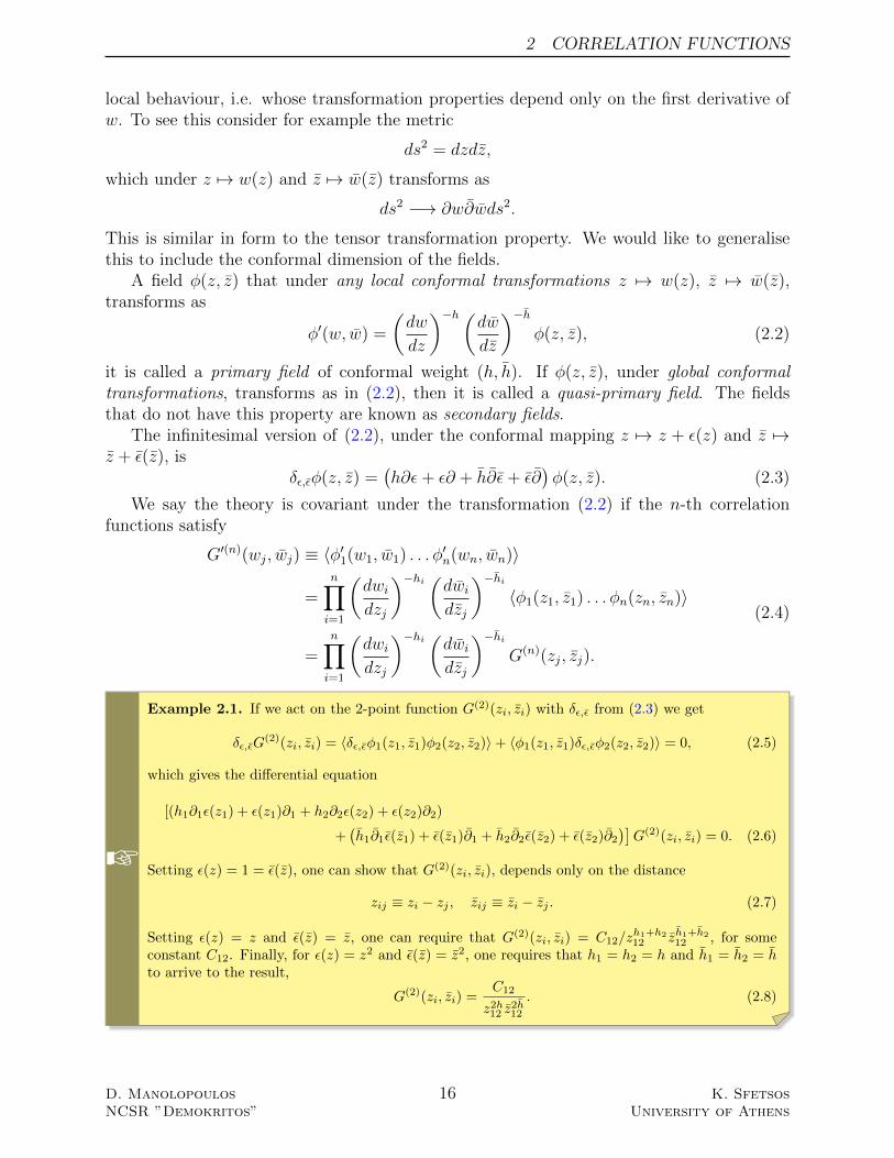
Example 2.1. If we act on the 2-point function G(2)(zi, zi) with δε,ε from (2.3) we get

δε,εG(2)(zi, zi) = 〈δε,εφ1(z1, z1)φ2(z2, z2)〉+ 〈φ1(z1, z1)δε,εφ2(z2, z2)〉 = 0, (2.5)

which gives the differential equation

[(h1∂1ε(z1) + ε(z1)∂1 + h2∂2ε(z2) + ε(z2)∂2)

+(h1∂1ε(z1) + ε(z1)∂1 + h2∂2ε(z2) + ε(z2)∂2

)]G(2)(zi, zi) = 0. (2.6)

Setting ε(z) = 1 = ε(z), one can show that G(2)(zi, zi), depends only on the distance

zij ≡ zi − zj , zij ≡ zi − zj . (2.7)

Setting ε(z) = z and ε(z) = z, one can require that G(2)(zi, zi) = C12/zh1+h212 zh1+h2

12 , for someconstant C12. Finally, for ε(z) = z2 and ε(z) = z2, one requires that h1 = h2 = h and h1 = h2 = hto arrive to the result,

G(2)(zi, zi) =C12

z2h12 z

2h12

. (2.8)



2.1 The Energy-Momentum Tensor 2 CORRELATION FUNCTIONS

In two dimensional CFTs, we can always take a basis of quasi-primary φi with fixedconformal weight and one can normalize their 2-point functions as

〈φi(z, z)φj(w, w)〉 =δij

(z − w)2hi(z − w)2hi. (2.9)

2.1 The Energy-Momentum Tensor

We would now like to explore the consequences of conformal invariance for correlation func-tions in a fixed domain (usually the entire complex plane). It is necessary to considertransformations which are not conformal everywhere, i.e. local conformal transformations.This brings in the energy-momentum tensor (or stress-energy tensor). The name energy-momentum tensor refers to Minkowski space-time while the name stress-energy tensor refersto the elastic properties of materials. In a slight abuse of notation we will use both names. Ina classical field theory it is defined as the Noether current which is conserved and symmetric,in response of the action S to a general infinitesimal transformation εµ(x),

δS = −

d2x T µν∂µεν = −

d2x T µν∂(µεν). (2.10)

This is valid even if the equations of motion are not satisfied. Then equations (1.8) and(1.9) imply that the corresponding variation of the action under an infinitesimal conformaltransformation is

δS =

d2x T µµ(Ω2 − 1) = 0, (2.11)

where Ω2 = 1− ∂νεν is not an arbitrary function. The tracelessness of T µν then implies theinvariance of the action under conformal transformations. Altogether, respectively in thatorder, the properties of the stress tensor which originate from invariance under, rotations,rescaling and its conservation law and when its position does not coincide with that of otherfields, are

T[µν] = 0, T µµ = 0, ∂µTµν = 0 (2.12)

i.e. symmetric, traceless and conserved. There is a quantum version of the above relationsdemonstrated by the so-called Ward identities that we will see in the next subsection. Therelations between its components Tαβ in complex (z, z) and Tµν in Cartesian (x, y) coordinatesare

Tzz = 14

(T11 − 2iT21 − T22) Tzz = 14

(T11 + 2iT21 − T22) Tzz = Tzz = 0Txx = Tzz + Tzz Tyy = −Txx Txy = i(Tzz − Tzz) = Tyx

(2.13)

b Exercise 2.2. Show this using the transformation property of Tµν , as well as table 1.

The conservation law gαγ∂γTαβ = 0, implies that

∂T = ∂T = 0. (2.14)



2.2 Ward Identities 2 CORRELATION FUNCTIONS

Therefore, the energy-momentum tensor splits into a holomorphic and an antiholomorphicpart and it is customary to write these parts as T ≡ T (z) ≡ Tzz and T ≡ T (z) ≡ Tzz,respectively. It will also be useful to define a renormalized version thereof by

T (z) ≡ −2πTzz, T (z) ≡ −2πTzz. (2.15)

2.2 Ward Identities

In this subsection we consider the consequences of a continuous symmetry transformation,explained in subsection 1.1, on the correlation functions

〈φ(x1) . . . φ(xn)〉 =1

Z

[Dφ] φ(x1) . . . φ(xn)e−S[φ], (2.16)

where Z is the vacuum functional. Under a continuous symmetry transformation of theaction and the integration measure the correlation functions of the theory are constrainedvia the so-called Ward identities. Since correlation functions are the main object of studyin a quantum theory, one may say, that the Ward identities are the quantum analog ofNoether’s theorem.

The variation of the action under a symmetry transformation δφ(x) = φ′(x) − φ(x) isgiven by1

δS =

d2x δL(φ, ∂µφ)

=

d2x

∂L∂φ

δφ+∂L

∂ (∂µφ)∂µ(δφ)

=

d2x

[∂L∂φ− ∂µ

∂L∂ (∂µφ)

]δφ+ ∂µ

(∂L

∂ (∂µφ)

) (2.17)

When the equations of motion are satisfied the term in the square brackets vanishes, so weare left with

δL = ∂µ

(∂L

∂ (∂µφ)

). (2.18)

However, for the transformation δφ to be a symmetry, the Lagrangian must change by atotal derivative δL = ∂µF

µ. Equating this with (2.18) we get the conserved current

∂µjµ = 0, (2.19)

with

jµ =∂L

∂ (∂µφ)δφ− F µ. (2.20)

In particular, one may show that under (1.22) and (1.23) the action transforms as

δS = −

d2x (jµ)a ∂µεa(x). (2.21)

1The arguments presented here apply also in d dimensions and not just two that we will keep using justfor the sake of argument.




Then the conservation law (2.19) simply follows from Noether’s theorem, i.e. if the fieldconfiguration obeys the classical equations of motion, the action is invariant under anyvariation of the fields for any position dependent parameters εa(x).

We consider now the infinitesimal symmetry transformation

δφ(x) ≡ φ′(x)− φ(x) = −iεa(x)T aφ(x), (εa(x) 1), (2.22)

acting on the correlation functions (2.16). Note that the positions are the same on both sidesand that the parameters εa(x) depend now on the position. Under such a local transformationthe action is not invariant and its variation δS = S ′ − S, is given by (2.21). Thus, one maywrite

〈φ(x1) . . . φ(xn)〉 (1)=

1

Z

[Dφ′] φ′(x1) . . . φ′(xn)e−S

′[φ′]

(2)=

1

Z

[Dφ′] φ(x1) . . . φ(xn) + δ(φ(x1) . . . φ(xn))e−(S[φ]+δS[φ])

(3)=

1

Z

[Dφ′] φ(x1) . . . φ(xn) + δ(φ(x1) . . . φ(xn))e−(S[φ]+

d2x ∂µ(jµ)aεa(x))

(4)= 〈φ′(x1) . . . φ′(xn)〉 −

d2x ∂µ〈(jµ)a φ(x1) . . . φ(xn)〉εa(x)

(2.23)

In step (1) we did not perform a real change of integration variables, we just renamedthe dummy integration variable φ → φ′. In step (2) we performed a change of functionalintegration variables and we assumed that the functional integration measure is invariantunder the local transformation (2.22), i.e. [Dφ′] = [Dφ]. In step (3) we integrated by parts(2.21) and substituted the result for δS. Finally, in step (4) we expanded to first order in εand used δφ(x) = φ′(x)− φ(x) where necessary. In conclusion the above yields

〈δφ(x1) . . . φ(xn)〉 =

d2x ∂µ〈(jµ)a φ(x1) . . . φ(xn)〉εa(x). (2.24)

On the other hand one may write the variation explicitly as

〈δφ(x1) . . . φ(xn)〉 = −in∑j=1

〈φ(x1) . . . Taφ(xj) . . . φ(xn)〉εa(xj)

= −i

d2x

n∑j=1

δ(x− xj)〈φ(x1) . . . Taφ(xj) . . . φ(xn)〉εa(x)

(2.25)

Finally, since (2.24) holds for an arbitrary infinitesimal function εa(x), one arrives at theWard identity for the current (jµ)a

∂µ〈(jµ)a (x)φ(x1) . . . φ(xn)〉 = −in∑j=1

δ(x− xj)〈φ(x1) . . . Taφ(xj) . . . φ(xn)〉 (2.26)




This identity says that the current (jµ)a is a conserved quantity, except when its positioncoincides with that of the other fields.

One can show a similar identity for the variation of the action with respect to the fields.⟨δS

δφ(x)φ(x1) . . . φ(xn)

⟩= −

n∑j=1

δ(x− xj)〈φ(x1) . . . φ(xn)〉 (2.27)

This is known as the Schwinger-Dyson equation which says that the classical equation ofmotion is satisfied by a quantum field inside a correlation function, as far as its space-timeargument differs from those of all other fields. We will use this later on to derive the equationof motion for the propagator of the free boson and the free fermion.

Z

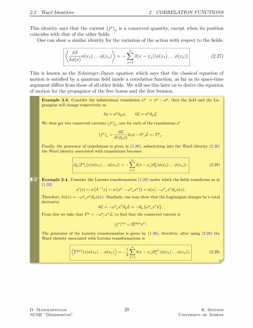
Example 2.3. Consider the infinitesimal translation xµ → xµ − aµ, then the field and the La-grangian will change respectively as

δφ = aµ∂µφ, δL = aµ∂µL.

We thus get two conserved currents (jµ)ν , one for each of the translations aν

(jµ)ν =∂L

∂ (∂µφ)∂νφ− δµνL =: Tµν .

Finally, the generator of translations is given in (1.28), substituting into the Ward identity (2.26)the Ward identity associated with translations becomes

∂µ〈Tµν(x)φ(x1) . . . φ(xn)〉 = −n∑j=1

δ(x− xj)∂jµ〈φ(x1) . . . φ(xn)〉. (2.28)

Example 2.4. Consider the Lorentz transformation (1.29) under which the fields transforms as in(1.33)

φ′(x) = φ(Λ−1x

)= φ

(xµ − ωµνxµ)

)= φ(x)− ωµνxν∂µφ(x).

Therefore, δφ(x) = −ωµνxν∂µφ(x). Similarly, one may show that the Lagrangian changes by a totalderivative

δL = −ωµνxν∂µL = −∂µ(ωµνx

νL).

From this we take that Fµ = −ωµνxνL, to find that the conserved current is

(jµ)νρ = 2Tµ[ρxν].

The generator of the Lorentz transformation is given by (1.36), therefore, after using (2.28) theWard identity associated with Lorentz transformations is

⟨T [µν](x)φ(x1) . . . φ(xn)

⟩= − i

2

n∑j=1

δ(x− xj)Sµνj 〈φ(x1) . . . φ(xn)〉. (2.29)




b

Exercise 2.5. Assuming that the dilation conserved current is

(jµ)D = Tµνxν ,

and knowing that the generator of dilations is as given by (1.38), find an expression for the associatedWard identity and by invoking (2.28) show that Ward identity for dilations can take the form

⟨Tµµ(x)φ(x1) . . . φ(xn)

⟩= −

n∑j=1

δ(x− xj)∆j〈φ(x1) . . . φ(xn)〉. (2.30)

Equations (2.28), (2.29) and (2.30) are the Ward identities associated with conformalinvariance.

2.2.1 Holomorphic form of the Ward Identities

We now use radial quantization2 on the complex plane, in order to derive Ward’s identities incomplex form. Consider an infinite cylinder of circumference L, with the time t ∈ R, runningalong the “flat” direction of the cylinder and space being compactified with a coordinatex ∈ [0, L], the points (0, t) and (L, t) being identified. If we continue to Euclidean space, thecylinder is described by a single coordinate w = x + it (or w = x− it). We then “explode”the cylinder onto the complex plane (or rather, the Riemann sphere) via the mapping

t2

t1

t

x

e2πiw/L−−−−→0

z

t2

t1

(2.31)

The remote past (t → −∞) is situated at the origin z = 0, whereas the remote future(t→ +∞) lies on the point at infinity on the Riemann sphere.

With the decomposition (2.14) of the energy-momentum tensor into holomorphic andantiholomorphic parts at hand, we can now define in radial quantization the conserved charge

Q =1

2πi

(dz T (z)ε(z) + dz T (z)ε(z)

), (2.32)

from the conserved current J(z, z) ≡ T (z)ε(z) + T (z)ε(z). The line integral is performedover some circle of fixed radius and our sign conventions are such that both the dz and thedz integrations are taken in the counter-clockwise sense (hence the symbol

). Note that

2In the operator formalism of CFT one distinguishes a time direction from a space direction. Thisis natural in Minkowski space-time, but somewhat arbitrary in Euclidian space-time. This allows one tochoose the space direction in more exotic ways, for instance along concentric circles centered at the origin.This choice of space and time leads to the so-called radial quantization of 2d-CFTs.




(2.32) is a formal expression that cannot be evaluated until we specify what other fields lieinside the contour.

Within radial quantization time ordering inside the definition of correlation functionsbecomes radial ordering. Products of two operators O1(z)O2(w), in Euclidean space quan-tization are only defined for |z| > |w|. Thus, we define the radial-order operator 3

R (O1(z)O2(w)) :=

O1(z)O2(w), |z| > |w|O2(w)O1(z), |z| < |w| . (2.33)

Consider now two holomorphic fields φ(z) and ψ(z) and then take the integral

I =

w

dz R (φ(z)ψ(w)) , (2.34)

with the integration contour encircling counterclockwise the point w. We now split theintegration contour into two fixed time circles:

w

z

−

w

z

=

w

z

, (2.35)

whose difference combines into a single integration about a contour drawn tightly aroundthe point w, which is our initial contour. Therefore, (2.34) becomes

w

dz R (φ(z)ψ(w)) =

(|z|>|w|

−|z|<|w|

)dz R (φ(z)ψ(w)) =

[dz φ(z), ψ(w)

]. (2.36)

Note that whenever we write a contour integral without specifying the contour of integrationit is understood that we integrate at a fixed time, i.e. along a circle centered at the origin.Integrating (2.36) over w we take[

dz φ(z),

dw ψ(w)

]=

0

dw

w

dz R (φ(z)ψ(w)) . (2.37)

The point for doing all this is that one can show (see exercise 2.6) that the variation ofa primary field φ(w, w), is given by the equal time commutator of the field with the chargeQ from (2.32)

δε,εφ(w, w) = [Q, φ(w, w)]

=1

2πi

(|z|>|w|

−|z|<|w|

)dz R (T (z)φ(w, w)) ε(z) + dz R

(T (z)φ(w, w)

)ε(z)

=

1

2πi

w

dz R (T (z)φ(w, w)) ε(z) + dz R

(T (z)φ(w, w)

)ε(z)

=(h∂ε+ ε∂ + h∂ε+ ε∂

)φ(w, w),

(2.38)

3The same definition holds but with a minus sign for fermionic operators.



2.3 Operator Product Expansion 2 CORRELATION FUNCTIONS

where in the last line we have substituted the desired result, equation (2.3). This is theso-called conformal Ward identity. To summarize:

δε,εφ(w, w) = [Q, φ(w, w)] =(h∂ε+ ε∂ + h∂ε+ ε∂

)φ(w, w). (2.39)

Inserting the holomorphic and antiholomorphic parts of (2.38), separately in a correlatorand using Cauchy’s formula one can deduce

〈T (z)φ1(w1, w1)...φn(wn, wn)〉 =n∑i=1

(hi

(z − wi)2+

∂iz − wi

)· 〈φ1(w1, w1)...φn(wn, wn)〉+ reg(z)

, (2.40)

where reg(z) is a regular function on the complex plane. A similar relation holds for T (z).

b

Exercise 2.6. Given the conformal Ward identity

δε,εφ(w, w) =1

2πi

(|z|>|w|

−|z|<|w|

)dz R (T (z)φ(w, w)) ε(z) + dz R

(T (z)φ(w, w)

)ε(z)

,

with the help of equations (2.36) and (2.37), convince yourself that it can be written as

δε,εφ(w, w) = [Q,φ(w, w)].

There is an easier way to derive the Ward identities (2.40) directly from equations (2.28),(2.29) and (2.30). This is the subject of the following exercise.

b

Exercise 2.7. Using the identity

δ(x) =1

π∂

1

z=

1

π∂

1

z,

find explicit expressions for the Ward identities (2.28), (2.29) and (2.30) in complex form, withthe n points xi described now by the 2n complex coordinates (wi, wi). Also for (2.29) it is more

convenient to multiply it by εµν (with εµν =(

0 i2

− i2

0

)totaly antisymmetric) and define si ≡ εµνSµνi ,

i.e. the spin of the field φi. Then by adding and subtracting the expressions you found for (2.29)and (2.30) and using (2.1) you must get

2π〈Tzzφ(w1, w1) . . . φ(wn, wn)〉 = −n∑j=1

∂hi

z − wi

2π〈Tzzφ(w1, w1) . . . φ(wn, wn)〉 = −n∑j=1

∂hi

z − wi

.

Inserting these relations to the complex expressions that you found for (2.28) deduce (2.40).

2.3 Operator Product Expansion

In section 2 we introduced correlation functions which reflect the infinite fluctuations ofa quantum field measured at a precise position. The operator product expansion (OPE)represents the product of two operators at different positions z and w respectively, by a sum




of terms, each being a single operator, well defined as z → w, multiplied by a (k-valued,with k = R or C) function of z−w, possibly diverging as z → w. This divergence embodiesthe infinite fluctuations as the two positions tent to each other. For example, consider thecorrelation function (2.9), then the OPE of two such fields will be of the form

φi(z, z)φj(w, w) ∼∑k

C kij (z − w)hk−hi−hj(z − w)hk−hi−hjφk(w, w), (2.41)

here C kij , are the operator product coefficients and are symmetric in i, j, k. In particular,

using the conformal Ward identity (2.40) we see that the OPE of the stress tensor with aprimary bulk field is4

T (z)φ(w, w) =

(h

(z − w)2+

∂

z − w

)φ(w, w) + reg(z − w), (2.42)

with a similar expression for T (z). The most general OPE for T (similarly for T ), consistentwith associativity is

T (z)T (w) =c/2

(z − w)4+

2

(z − w)2T (w) +

∂

z − wT (w) + reg(z − w). (2.43)

The constant c is called the central charge and fixes the properties of the CFT. We alsosee that the conformal dimension of T is h = 2. The OPE of T with T has no poles.A consequence of (2.43) is the transformation behaviour of T (z) under a conformal mapz 7→ w(z)

T (z) =

(dw

dz

)2

T (w) +c

12w; z , (2.44)

where

w; z := w′′′(z)w′(z)

− 32

(w′′(z)w′(z)

)2

, (2.45)

is the Schwarzian derivative. Thus, we see that the energy momentum tensor is not a primaryfield. However, the Schwarzian derivative of (1.49) vanishes. This needs to be so, since T (z)is a quasi-primary field.

2.3.1 The Free Boson

The simplest example of a CFT is that of the real free massless scalar field φ(x, t), usuallycalled the free boson. In two dimensions its dynamics (in the massless case) are describedby the action

S[φ] =g

2

d2x ∂µφ∂

µφ, g ∈ R. (2.46)

4Note that whenever we write OPEs it is understood that they make sense only inside a correlator, wethus drop 〈−〉.




We are interested in calculating the two point function (or propagator) G(2)(x, y) ≡〈φ(x)φ(y)〉. From the Schwinger-Dyson equations (2.27) the propagator satisfies the differ-ential equation

− g∂2xG

(2)(x, y) = δ(x− y). (2.47)

b Exercise 2.8. Show this by integrating by parts (2.46), then find δSδφ(x) and use the Schwinger-Dyson

equations (2.27) to arrive to (2.47).

Because of rotational and translational invariance, the propagator will be a function ofthe distance r = |x− y|. Integrating within a disc of radius r centered around y we get thedifferential equation

1 = 2πg

r

0

dρ ρ

−1

ρ∂ρ(ρG′(2)(ρ)

)= −2πgrG′(2)(r), (2.48)

whose solution is

〈φ(x)φ(y)〉 = − 1

4πgln2(x− y), (2.49)

or in complex coordinates

〈φ(z)φ(w)〉 = − 1

4πgln(z − w). (2.50)

Note that the field φ(z) is not itself a primary field because of the logarithm in (2.50), butits derivative has an OPE

〈∂φ(z)∂φ(w)〉 = − 1

4πg

1

(z − w)2. (2.51)

The associated energy momentum tensor is given by

Tµν = g

(∂µφ∂νφ−

1

2ηµν∂ρφ∂

ρφ

), (2.52)

which, after using (2.15) and Table 1, it can be written in its quantum version as

T (w) = −2πg :∂φ(w)∂φ(w):

(1)= −2πg lim

z→w(∂φ(z)∂φ(w)− 〈∂φ(z)∂φ(w)〉)

(2)= −2πg lim

z→w

(∂φ(z)∂φ(w) +

1

4πg

1

(z − w)2

).

(2.53)

In step (1) we used point splitting and Wick’s theorem (see Appendix A.1) to rewrite :∗: =R(∗) − 〈∗〉, while in step (2) we used equation (2.51). It is also understood that wheneverwe write the product A(z)B(w), of two operators, we mean the radially ordered productR(A(z)B(w)). As expected, the normal ordering :∗: appears to ensure the vanishing of its




vacuum expectation value. The OPE of T (z) with itself can be calculated as follows

T (z)T (w) = (2πg)2 :∂φ(z)∂φ(z): :∂φ(w)∂φ(w):

(1)= (2πg)2

(2〈∂φ(z)∂φ(w)〉2 + 4〈∂φ(z)∂φ(w)〉 :∂φ(z)∂φ(w):

)(2)=

1/2

(z − w)4− 4πg

(z − w)2:∂φ(z)∂φ(w):

(3)=

1/2

(z − w)4− 4πg

(z − w)2:(∂φ(w) + (z − w)∂2φ(w) +O

((z − w)2

))∂φ(w):

(4)=

1/2

(z − w)4+

2T (w)

(z − w)2+∂T (w)

z − w

.

(2.54)

In step (1) we used Wick’s theorem, while the factors of 2 and 4 arise as a result of countingall possible combinations of terms. In step (2) we used (2.51), in step (3) we Taylor expandedthe z-dependent term in :∂φ(z)∂φ(w): around the point w, and finally, in step (4) we used(2.51) to observe that ∂T (w) = :∂2φ(w)∂φ(w): and ignored the O ((z − w)2) terms sincethey are non singular. Comparing the result with (2.43) we observe that the central chargefor the free boson is c = 1.

Another variation of the above is to consider a free boson with OPE

φ(z)φ(w) = − ε

4πgln(z − w), (2.55)

with energy momentum tensor and central charge given by

T (z) = −2πgε :∂φ(z)∂φ(z): +Q∂2φ(z), c = 1 + 48πgεQ2. (2.56)

The extra term proportional to Q ∈ R in T (z) above is a total derivative not affecting theenergy momentum tensor being a conformal generator. The value of ε indicates whether theboson is spacelike (ε = 1) or timelike (ε = −1). The effect of the extra term in (2.56) is toshift c > 1 for ε = 1 or c < 1 for ε = −1. This is an important point because the valueof the central charge indicates the unitarity of the theory, this will be briefly explained insubsection 3.2. We thus see that spacelike bosons always produce unitary representations.As for Q we will interpret it as a background charge at infinity later on when we will talkabout vertex operators. It is for specific values of Q at c < 1 that fit in the Kac table thatthe theory is unitary.

b Exercise 2.9. Show that for T (z) as given in (2.56) and using the OPE (2.55) that the centralcharge is indeed as given in (2.56). What can you say about unitarity if Q→ iQ?

2.3.2 The Free Fermion

The action for a free massless Majorana fermion in two Euclidean dimensions (ηµν = δµν) isgiven by

S[Ψ] =g

2

d2x Ψ/∂Ψ, (2.57)




where we have used Dirac’s slash notation with /∂ ≡ γµ∂µ and have defined the Dirac adjointΨ ≡ Ψ†γ0. We recall that a Majorana spinor is a real spinor Ψ = Ψ∗. The gamma matricessatisfy the Clifford algebra relation

γµ, γν = 2ηµν . (2.58)

In two Euclidean dimensions a representation of the gamma matrices is given by

γ0 =

(0 11 0

), γ1 =

(0 −ii 0

). (2.59)

Therefore, one can calculate

γ0/∂ = γ0(γ0∂0 + γ1∂1

)=

(0 ∂x − i∂y

∂x + i∂y 0

)= 2

(0 ∂∂ 0

). (2.60)

Thus, if we write Ψ =(ψ, ψ

)T, the action (2.57) can be written in complex form as

S[ψ, ψ] = g

d2x

(ψ∂ψ + ψ∂ψ

), (2.61)

whose equations of motion read ∂ψ = 0 = ∂ψ (i.e. the Cauchy-Riemann equations (1.42)).

Once more, we are interested in finding the propagator G(2)ij ≡ 〈ψi(z, z)ψj(w, w)〉, where here

i, j = 1, 2. From the Schwinger-Dyson equations (2.27) one can show that the propagatorsatisfies the equation of motion

gδ(x− y)(γ0γµ

)ik∂µG

(2)kj (x, y) = δijδ(x− y), (2.62)

or in complex form

2g

(∂ 00 ∂

)(G

(2)11 G

(2)

12

G(2)

21G

(2)

22

)=

1

π

(∂ 1z−w 0

0 ∂ 1z−w

), (2.63)

where the factor of 1/π comes from the identity δ(x) = 1π∂ 1z

= 1π∂ 1z. From the equations of

motion (2.63) one can read off the solution

〈ψ(z)ψ(w)〉 =1

2πg

1

z − w, 〈ψ(z)ψ(w)〉 =

1

2πg

1

z − w, 〈ψ(z)ψ(w)〉 = 0 = 〈ψ(z)ψ(w)〉.

(2.64)Comparing this to (2.9) we see that the conformal dimension of the fermions is indeed hψ = 1

2.

b

Exercise 2.10. Consider now two real fermions ψi, i = 1, 2 from which we form the complexcombinations

ψ± =ψ1 ± iψ2√

2.

Show that the OPE of the complex fermion with itself is

ψ+(z)ψ−(w) =1

2πg

1

z − w.



3 THE OPERATOR FORMALISM

To calculate the energy momentum tensor we use the Lagrangian from (2.61) and employthe canonical form

Tαβ =∂L

∂(∂αψδ)gγβ∂γψδ − gαβL, (2.65)

where α, β, γ, δ = z, z and ψδ are the components of Ψ =(ψ, ψ

). The above expression for

Tαβ for fermions can simplify even further if we impose the equations of motion which arefirst order, a trick which we cannot use in the case of a scalar field whose equations of motionare second order in derivatives. This means that we can set L = 0 in Tαβ, we are thus leftwith

Tαβ =∂L

∂(∂αψδ)gγβ∂γψδ. (2.66)

Then one may show (see exercise 2.11) that the holomorphic part (similarly the antiholo-morphic part) of the energy momentum tensor is given by

T (z) = −πg :ψ(z)∂ψ(z): . (2.67)

b Exercise 2.11. Using equation (2.66) and the Lagrangian from the action (2.61) calculate thecomponents T zz, T zz, T zz. Then from (2.15) show equation (2.67).

As in the case of the free boson one can perform a similar calculation for the free fermionfor the OPE of T (z) with itself (see expertise 2.12) to find

T (z)T (w) =1/4

(z − w)4+

2T (w)

(z − w)2+∂T (w)

z − w, (2.68)

which satisfies (2.43) for c = 1/2.

b

Exercise 2.12. Show equation (2.68) using

〈∂ψ(z)ψ(w)〉 = − 1

2πg

1

(z − w)2, 〈ψ(z)∂ψ(w)〉 =

1

2πg

1

(z − w)2, 〈∂ψ(z)∂ψ(w)〉 = − 1

πg

1

(z − w)3.

Exercise 2.13. Show that for the complex free fermion considered in exercise 2.10 the energymomentum tensor is given by

T (z) = −πg∑i

:ψi(z)∂ψi(z): = −πg( :ψ+(z)∂ψ−(z): + :ψ−(z)∂ψ+(z): )

and has central charge c = 1.

3 The Operator Formalism

In the operator formalism, in a nutshell, a 2d CFT is determined by the following data:

♣ A space of states5 H, a C-vector space, as well as, a space of fields F , an S-gradedvector space F =

⊕∆∈SF (∆), with S, the spectrum, a discrete subset of R and

0 < dim F (∆) <∞.5May or may not be a Hilbert space. There are examples where the space of states is not a Hilbert space,

as the inner product is not positive-definite.



3.1 The Virasoro Algebra 3 THE OPERATOR FORMALISM

♠ Its correlation functions, which are defined for collections of vectors in F , togetherwith an isomorphism ι : F → H, the state-field correspondence, in the sense that afield inserted at a point can be thought of as a state and vice versa.

As we have seen, two-dimensional CFTs contain an infinite variety of coordinate transfor-mations that although not everywhere well defined, are locally conformal and they are holo-morphic mappings from the complex plane to itself. The corresponding infinite-dimensionalsymmetry algebra of the CFT is related to a preferred subspace F0 of F , that is charac-terised by the property that it only allows holomorphic dependance of the coordinates forthe correlation functions.

The OPE is associative and if we consider the case of two holomorphic fields φ1, φ2 ∈ F0,then the associativity of the OPE implies that the states in F0 form a representation of theso-called vertex operator algebra V (to be defined later on). The same also holds for thevertex operator algebra associated to the anti-holomorphic fields and one can decompose thewhole space F (or H) as

H =⊕i,∈I

(Ri ⊗C R

)⊕Mi , (3.1)

where I denotes the set indexing the irreducible representations of V , Ri | i ∈ I thecorresponding representations and Mi ∈ N denotes the multiplicity with which the tensorproduct Ri ⊗C R occurs in H. These statements will make more sense later on.

We must also assume the existence of a vacuum state |0〉 ∈ H upon which the spaceof states is constructed. In free field theories, the vacuum may be defined as the stateannihilated by the positive frequency part of the field [BYB, Sect. 2.1 & 6.1.1].

i The sl(2)-invariant vacuum

To be precise we should call |0〉 the sl(2)-invariant vacuum, since e.g. for a non-unitary theory on a cylinder, it is not the state of lowest energy and thus not thereal vacuum. It will always be clear from the context whether “vacuum” refers tothe state of lowest energy or the sl(2)-invariant state |0〉. Moreover, the expressions,correlation function, n-point function, amplitude and vacuum-expectation value allrefer to the (radially ordered) vacuum-expectation value 〈0| . . . |0〉 with respect to thesl(2)-invariant vacuum.

3.1 The Virasoro Algebra

We can now define the action of the stress tensor T and its antiholomorphic counterpart Ton the space of states H, via their mode expansion. In general, a holomorphic (similarly anantiholomorphic) field φ(z) of conformal dimension (h, 0) can be mode expanded as follows

φ(z) =∑n∈Z

z−n−hφn, φn =1

2πi

dz zn+h−1φ(z). (3.2)



3.1 The Virasoro Algebra 3 THE OPERATOR FORMALISM

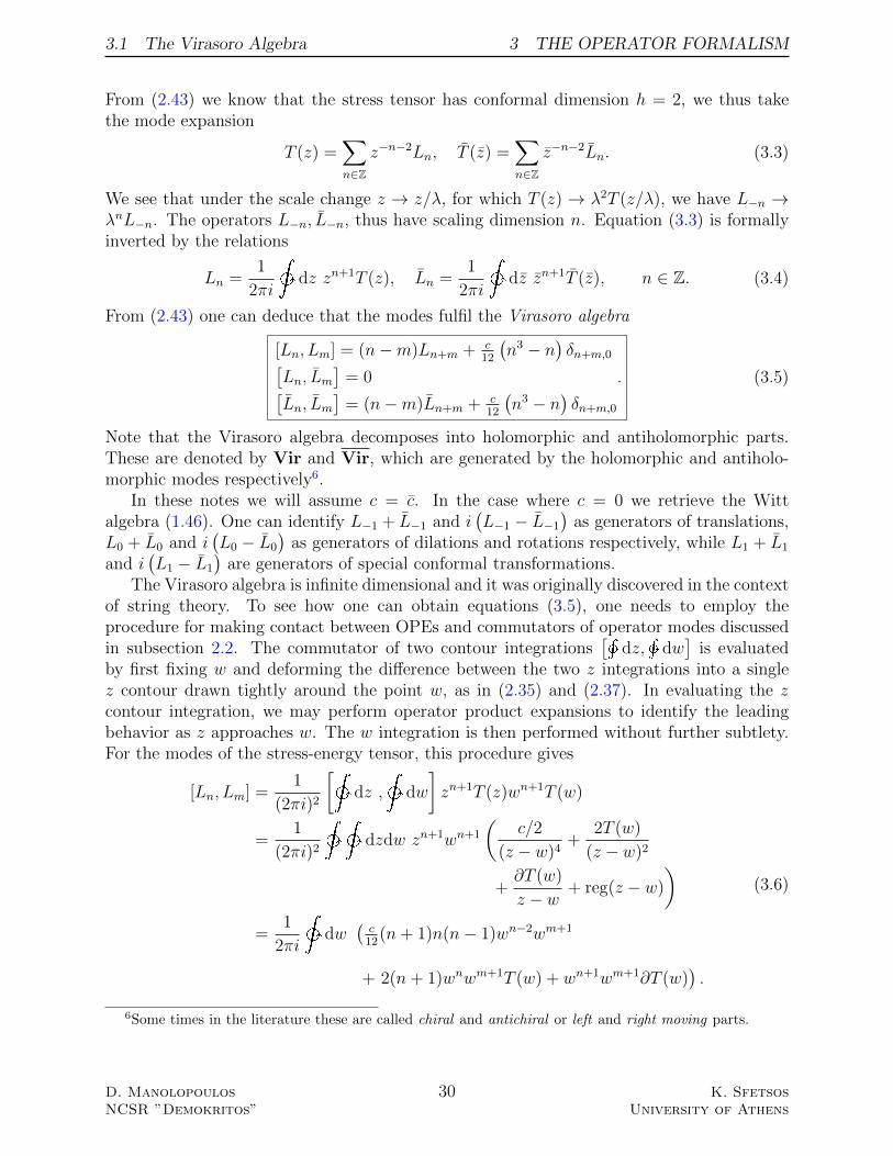
From (2.43) we know that the stress tensor has conformal dimension h = 2, we thus takethe mode expansion

T (z) =∑n∈Z

z−n−2Ln, T (z) =∑n∈Z

z−n−2Ln. (3.3)

We see that under the scale change z → z/λ, for which T (z) → λ2T (z/λ), we have L−n →λnL−n. The operators L−n, L−n, thus have scaling dimension n. Equation (3.3) is formallyinverted by the relations

Ln =1

2πi

dz zn+1T (z), Ln =

1

2πi

dz zn+1T (z), n ∈ Z. (3.4)

From (2.43) one can deduce that the modes fulfil the Virasoro algebra

[Ln, Lm] = (n−m)Ln+m + c12

(n3 − n

)δn+m,0[

Ln, Lm]

= 0[Ln, Lm

]= (n−m)Ln+m + c

12

(n3 − n

)δn+m,0

. (3.5)

Note that the Virasoro algebra decomposes into holomorphic and antiholomorphic parts.These are denoted by Vir and Vir, which are generated by the holomorphic and antiholo-morphic modes respectively6.

In these notes we will assume c = c. In the case where c = 0 we retrieve the Wittalgebra (1.46). One can identify L−1 + L−1 and i

(L−1 − L−1

)as generators of translations,

L0 + L0 and i(L0 − L0

)as generators of dilations and rotations respectively, while L1 + L1

and i(L1 − L1

)are generators of special conformal transformations.

The Virasoro algebra is infinite dimensional and it was originally discovered in the contextof string theory. To see how one can obtain equations (3.5), one needs to employ theprocedure for making contact between OPEs and commutators of operator modes discussedin subsection 2.2. The commutator of two contour integrations

[dz,

dw]

is evaluatedby first fixing w and deforming the difference between the two z integrations into a singlez contour drawn tightly around the point w, as in (2.35) and (2.37). In evaluating the zcontour integration, we may perform operator product expansions to identify the leadingbehavior as z approaches w. The w integration is then performed without further subtlety.For the modes of the stress-energy tensor, this procedure gives

[Ln, Lm] =1

(2πi)2

[dz ,

dw

]zn+1T (z)wn+1T (w)

=1

(2πi)2

dzdw zn+1wn+1

(c/2

(z − w)4+

2T (w)

(z − w)2

+∂T (w)

z − w+ reg(z − w)

)=

1

2πi

dw

(c

12(n+ 1)n(n− 1)wn−2wm+1

+ 2(n+ 1)wnwm+1T (w) + wn+1wm+1∂T (w)).

(3.6)

6Some times in the literature these are called chiral and antichiral or left and right moving parts.



3.2 Highest Weight Representations 3 THE OPERATOR FORMALISM

Integrating the last term by parts and combining with the second term gives (n−m)wn+m+1T (w),so performing the w integration, produces the required result.

b Exercise 3.1. Do the missing steps described above to show the commutator of Vir.

The vacuum state |0〉 ∈ H must be invariant under global conformal transformations.This means that it must be annihilated by L−1,0,1 and L−1,0,1. This, however, can be recoveredby the condition that T (z)|0〉 and T (z)|0〉 are well defined as z, z → 0, which implies

Ln|0〉 = 0, Ln|0〉 = 0, n ≥ −1. (3.7)

Performing the corresponding contour integral with (2.42), we get the commutation relations

[Ln, φ(w, w)] = h(n+ 1)wnφ(w, w) + wn+1∂φ(w, w)[Ln, φ(w, w)

]= h(n+ 1)wnφ(w, w) + wn+1∂φ(w, w)

. (3.8)

b Exercise 3.2. Show this using (2.36) and the OPE (2.42).

From the state-field correspondence ♠ we see that when primary fields act on the vacuum,create asymptotic states

|φin〉 = limz,z→0

φ(z, z)|0〉. (3.9)

After applying the relations (3.8) to the asymptotic state

|h, h〉 ≡ φ(0, 0)|0〉, (3.10)

we takeL0|h, h〉 = h|h, h〉, L0|h, h〉 = h|h, h〉. (3.11)

Thus, |h, h〉 is an eigenstate of the Hamiltonian7. Similarly,

Ln|h, h〉 = Ln|h, h〉 = 0, n > 0. (3.12)

b Exercise 3.3. Show equations (3.11) and (3.12) by direct application of (3.8) on the vacuum state|0〉.

3.2 Highest Weight Representations

Highest weight representation are familiar to physicists through the theory of angular mo-mentum. Just as the energy eigenstates of the Hamiltonian of a rotationally invariant systemfall into irreducible representations of su(2), in a conformaly invariant theory the energyeigenstates of the Hamiltonian fall into representation of the Virasoro algebra (the localconformal algebra). The way one may construct these representations is similar to the su(2)case. The only difference here is that the Virasoro algebra is infinite dimensional and thuswe are dealing with infinite dimensional representations. However, one may overcome this by

7As will be seen later, the Hamiltonian is proportional to L0 + L0 − c12 .




passing to a finite dimensional subspace spanned by highest weight vectors, called a Vermamodule. The name module is just another name for representation space. Then the associ-ated representations (which can be seen as vectors in the Verma module) are called highestweight representations.

From the Virasoro algebra (3.5) we see that no pair of generators commute, so one canchoose L0 to be diagonal in the Verma module. From the defining relations of Vir it is easyto see that

[L0, L±n] = ∓nLn, n > 0. (3.13)

Thus, Ln is a lowering operator and L−n is a raising operator. For a state |h〉 to be a highestweight state one has8

Ln|h〉 = Ln|h〉 = 0, n > 0, (3.14)

which is compatible with (3.12). This state is, of course, the asymptotic state (3.10) createdby applying a primary field φ(0) of dimension h on the vacuum |0〉. One can construct morestates in the Verma module by applying the raising operators L−n in all possible ways

n∏i=1

L−ki |h〉, 1 ≤ k1 ≤ . . . ≤ kn. (3.15)

Recall that since L0|h〉 = h|h〉, then the above state has an L0 eigenvalue

h′ = h+n∑i=1

ki ≡ h+N, (3.16)

where N =∑n

i=1 ki is called the level of the state. The states in (3.15) are called descendantstates of the asymptotic state |h〉 and (3.15) constitutes a basis for the Verma module atlevel N . Table 2 shows the lowest states of a Verma module.

Level Dimension State

0 h |h〉1 h+ 1 L−1|h〉2 h+ 2 L−2|h〉, L2

−1|h〉3 h+ 3 L−3|h〉, L−1L−2|h〉, L3

−1|h〉4 h+ 4 L−4|h〉, L−1L−3|h〉, L2

−1L−2|h〉, L2−2|h〉, L4

−1|h〉...

......

N h+N p(N) states

Table 2: Lowest states of the Verma module.

In the table p(N) denotes the partition of the integer N generated by the function

1

ϕ(q):=

1∏∞n=1(1− qn)

=∞∑n=0

p(n)qn,(q ≡ e2πiτ

), (3.17)

8This is rather a “lowest” weight state because it is annihilated by Ln rather than L−n but it is customaryin many textbooks to be called as a “highest” weight state.




where ϕ(q) is the Euler function and τ ∈ C.

b Exercise 3.4. Show that the L0 eigenvalue of (3.15) is indeed as given by (3.16) by acting with L0

and using (3.13) to commute it past the L−ki ’s.

The inner product of two highest weight states |i〉 and |j〉, simply is

〈i|j〉 = δij. (3.18)

If we Hermitian conjugate T and T and restricting to the real surface z = z∗, we get

L†n = L−n, L†n = L−n. (3.19)

This relation together with the Virasoro algebra (3.5) and highest weight condition (3.14)can be used to write the inner product of an arbitrary pair of fields in terms of the innerproduct of primary fields.

bExercise 3.5. Show (3.19) by first Hermitian conjugating (3.3) on the real surface z = z∗ and thenusing the fact that

φ(z)† = z−2hφ

(1

z

).

One can define an inner product on the Verma module using the Hermitian conjugate(3.19). If we consider the states

m∏i=1

L−ki |h〉,n∏i=1

L−li|h〉, (3.20)

then their inner product simply is

〈h|1∏

i=m

Lki

n∏i=1

L−li|h〉. (3.21)

A similar analysis can be done for the Verma modules associated with the antiholomorphicgenerator Ln of Vir. Thus, we have seen that the set of modes of the holomorphic part ofthe stress tensor Ln | n ∈ Z generate the holomorphic representations Ri | i ∈ I, whilethe set of modes of the antiholomorphic part of the stress tensor Ln | n ∈ Z generate theantiholomorphic representations R | ∈ I. However, since the two parts decouple, inorder to take the physical space of states one needs to take tensor products of the aboverepresentations. Thus the space of states decomposes into highest weight representations ofVir⊕Vir of the form (3.1).

We saw that each module is spanned by a highest weight state |h, h〉 and an infinite setof descendent states of the form Lm1 . . . Ln1 . . . |h, h〉, with all m,n < 0. Once we know thecentral charge c, of the theory and the conformal weights

(h, h), of all primary fields, we can

construct the space of states. However, some care has to be taken in the construction of abasis, since not all products of L’s and L’s are linearly independent.

Furthermore, there will be states |χ〉 in the Verma module which are of the form (3.15)and which are also annihilated by Ln for all n > 0

Ln|χ〉 = 0, (n > 0). (3.22)




A state other than the highest weight state that is annihilated by Ln for all n > 0 is calleda null state. Null states are orthogonal to all the other states in the Verma module and thusthey form a submodule. In particular for a null state we have 〈χ|χ〉 = 0. A Verma modulewhich contains one or more null states is reducible. One can construct an irreducible Vermamodule by quotienting out this null submodule.

Z

Example 3.6. There are many such states, to construct an example just consider the followingstate at level 2

|χ〉 =

(L−2 −

3

2(2h+ 1)L2−1

)|h〉, with c =

2h(5− 8h)

2h+ 1

and |h〉 a highest weight state, then for n ≥ 0 we have

Ln|χ〉 =

([Ln, L−2]− 3

2(2h+ 1)[Ln, L

2−1]

)|h〉

=

([Ln, L−2]− 3

2(2h+ 1)(L−1[Ln, L−1] + [Ln, L−1]L−1)

)|h〉

This can only be non-zero for n = 0. Thus we find that L0|χ〉 = 2|χ〉. Next we see that 〈χ|h〉 =

〈h|(L−2 − 3

2(2h+1)L2−1

)†|h〉 = 0.

From the above example we see that if we calculate some amplitude between two physicalstates 〈h′|h〉 we can shift |h〉 → |h〉+ |χ〉. The new state is still physical but the amplitudewill remain the same - for any other choice of physical state |h′〉. In string theory, this isa stringy gauge symmetry whereby two physical states are equivalent if their difference is anull state. This turns out to be the origin of Yang-Mills and other gauge symmetries withinstring theory.

bExercise 3.7. Consider the following state at level 2

|χ〉 =(L−2 + ηL2

−1

)|h〉.

Tune η and h so that |χ〉 is a null state. Hint: The conditions L1|χ〉 = L2|χ〉 = 0 are sufficient forthis, since it then follows from the Virasoro algebra that Ln|χ〉 = 0, for n > 2.

Finally, to conclude this subsection, a representation of Vir (similarly of Vir) is said tobe unitary if it contains no negative norm states (known as ghosts in string theory). Forinstance, one can find a simple bound on the values of the central charge c and on the highestweight h in order for the representations to be unitary by considering the norm

〈h|LnL−n|h〉 =(

2nh+c

12n(n2 − 1)

)〈h|h〉. (3.23)

We see that if c < 0 this becomes negative for n sufficiently large. Therefore, all represen-tations with negative central charge are nonunitary. Furthermore, if n = 1 we see that allrepresentations with h < 0 are also nonunitary.

b Exercise 3.8. Show equation (3.23).

There is a general formula for one to decide whether or not a representation is unitarydue to Kac, known as the Kac determinant, however, it is beyond the scope of these notes to



3.3 The Free Boson 3 THE OPERATOR FORMALISM

go into more details so we will not reproduce it here. We will simply mention that wheneverthis determinant is negative then the representation is nonunitary. The big success of CFTin the study of two dimensional systems is due in great part to the knowledge of the Kacdeterminant. This formula is of central importance in the theory of minimal models butlets not go further into these matters. What is important for our purposes is that one canshow that all representations with c ≥ 1 and h ≥ 0 are unitary. One can also find unitaryrepresentations in the regions where c ∈ (0, 1) and h > 0, but this is not always the case.There is a formula for c, h for one to decide which representation are unitary known as Kactable but we will not need it here. For those interested see [BYB, Sec. 7.2].

3.3 The Free Boson

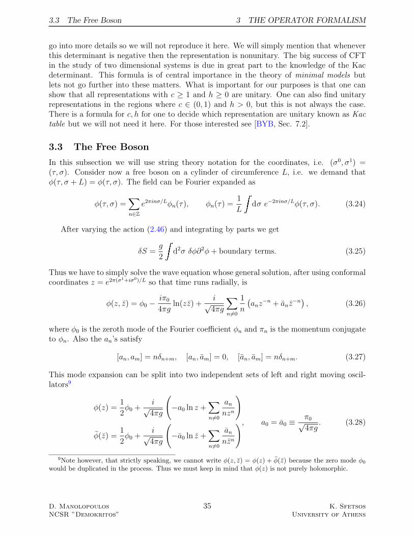
In this subsection we will use string theory notation for the coordinates, i.e. (σ0, σ1) =(τ, σ). Consider now a free boson on a cylinder of circumference L, i.e. we demand thatφ(τ, σ + L) = φ(τ, σ). The field can be Fourier expanded as

φ(τ, σ) =∑n∈Z

e2πinσ/Lφn(τ), φn(τ) =1

L

dσ e−2πinσ/Lφ(τ, σ). (3.24)

After varying the action (2.46) and integrating by parts we get

δS =g

2

d2σ δφ∂2φ+ boundary terms. (3.25)

Thus we have to simply solve the wave equation whose general solution, after using conformalcoordinates z = e2π(σ1+iσ0)/L so that time runs radially, is

φ(z, z) = φ0 −iπ0

4πgln(zz) +

i√4πg

∑n6=0

1

n

(anz

−n + anz−n) , (3.26)

where φ0 is the zeroth mode of the Fourier coefficient φn and πn is the momentum conjugateto φn. Also the an’s satisfy

[an, am] = nδn+m, [an, am] = 0, [an, am] = nδn+m. (3.27)

This mode expansion can be split into two independent sets of left and right moving oscil-lators9

φ(z) =1

2φ0 +

i√4πg

(−a0 ln z +

∑n6=0

annzn

)

φ(z) =1

2φ0 +

i√4πg

(−a0 ln z +

∑n6=0

annzn

), a0 = a0 ≡π0√4πg

. (3.28)

9Note however, that strictly speaking, we cannot write φ(z, z) = φ(z) + φ(z) because the zero mode φ0

would be duplicated in the process. Thus we must keep in mind that φ(z) is not purely holomorphic.



3.3 The Free Boson 3 THE OPERATOR FORMALISM

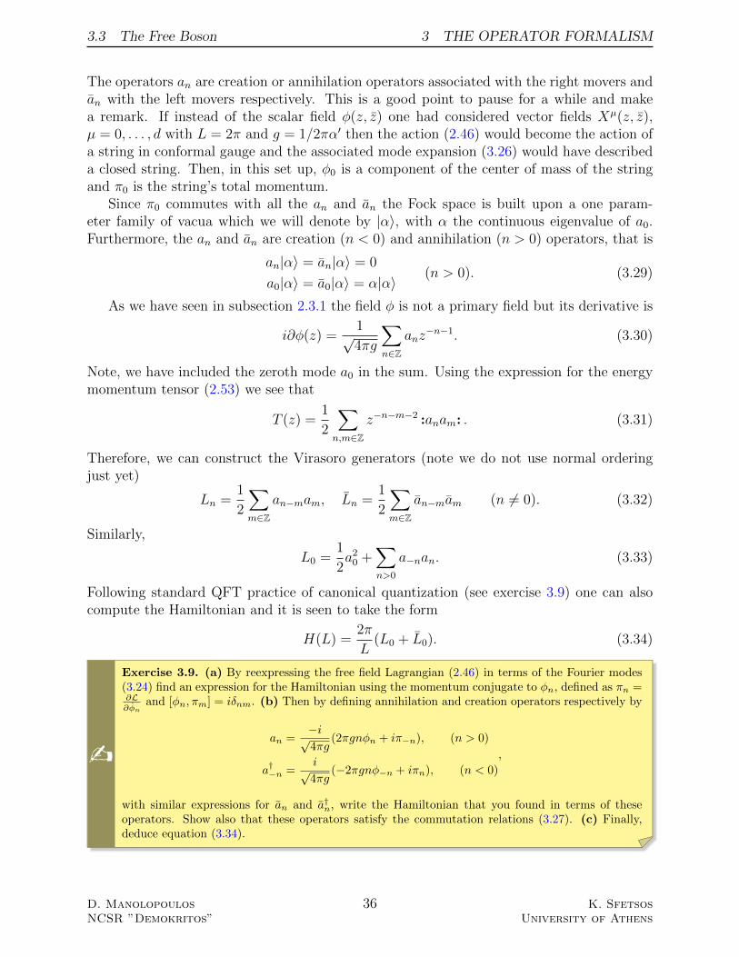
The operators an are creation or annihilation operators associated with the right movers andan with the left movers respectively. This is a good point to pause for a while and makea remark. If instead of the scalar field φ(z, z) one had considered vector fields Xµ(z, z),µ = 0, . . . , d with L = 2π and g = 1/2πα′ then the action (2.46) would become the action ofa string in conformal gauge and the associated mode expansion (3.26) would have describeda closed string. Then, in this set up, φ0 is a component of the center of mass of the stringand π0 is the string’s total momentum.

Since π0 commutes with all the an and an the Fock space is built upon a one param-eter family of vacua which we will denote by |α〉, with α the continuous eigenvalue of a0.Furthermore, the an and an are creation (n < 0) and annihilation (n > 0) operators, that is

an|α〉 = an|α〉 = 0

a0|α〉 = a0|α〉 = α|α〉(n > 0). (3.29)

As we have seen in subsection 2.3.1 the field φ is not a primary field but its derivative is

i∂φ(z) =1√4πg

∑n∈Z

anz−n−1. (3.30)

Note, we have included the zeroth mode a0 in the sum. Using the expression for the energymomentum tensor (2.53) we see that

T (z) =1

2

∑n,m∈Z

z−n−m−2 :anam: . (3.31)

Therefore, we can construct the Virasoro generators (note we do not use normal orderingjust yet)

Ln =1

2

∑m∈Z

an−mam, Ln =1

2

∑m∈Z

an−mam (n 6= 0). (3.32)

Similarly,

L0 =1

2a2

0 +∑n>0

a−nan. (3.33)

Following standard QFT practice of canonical quantization (see exercise 3.9) one can alsocompute the Hamiltonian and it is seen to take the form

H(L) =2π

L(L0 + L0). (3.34)

b

Exercise 3.9. (a) By reexpressing the free field Lagrangian (2.46) in terms of the Fourier modes(3.24) find an expression for the Hamiltonian using the momentum conjugate to φn, defined as πn =∂L∂φn

and [φn, πm] = iδnm. (b) Then by defining annihilation and creation operators respectively by

an =−i√4πg

(2πgnφn + iπ−n), (n > 0)

a†−n =i√4πg

(−2πgnφ−n + iπn), (n < 0)

,

with similar expressions for an and a†n, write the Hamiltonian that you found in terms of theseoperators. Show also that these operators satisfy the commutation relations (3.27). (c) Finally,deduce equation (3.34).



3.4 Vertex Operators 3 THE OPERATOR FORMALISM

Of course, the :Ln: ’s satisfy the Virasoro algebra. One can perform a direct calculationbut it is notoriously complicated and messy. We will only sketch the proof of how one mayproceed in an alternative way. First one calculates the commutator [Ln, Lm] without worryingabout normal orderings to find that it obeys the Witt algebra (1.46). When consideringnormal ordering we must generalize the commutator to

[ :Ln: , :Lm: ] = (n−m) :Ln+m: + C(n)δn+m,0. (3.35)

The easiest way to determine the C(n) is to note the following. First one imposes the Jacobiidentity

[ :Lk: , [ :Lm: , :Ln: ]] + [ :Lm: , [ :Ln: , :Lk: ]] + [ :Ln: , [ :Lk: , :Lm: ]] = 0. (3.36)

If we impose that k +m+ n = 0 with k,m, n 6= 0 (so that no pair of them adds up to zero)then this reduces to

(m− n)C(k) + (n− k)C(m) + (k −m)C(n) = 0.

Picking k = 1 and m = −n − 1 and noting that by definition C(n) is odd, we learn thatC(0) = 0 and

C(n+ 1) =(n+ 2)C(n)− (2n+ 1)C(1)

n− 1. (3.37)

This is just a difference equation and given C(2) it will determine C(n) for n > 1 (notethat it can’t determine C(2) given C(1)). We can look for a solution to this by consideringpolynomials. Since it must be odd in n the simplest guess is

C(n) = c1n3 + c2n, c1, c2 ∈ R. (3.38)

Note that if we shift L0 by a constant l then C(n) is shifted by 2nl. This means that we canchange the value of c2. Therefore we will fix it to be c1 = −c2. Finally we must calculate c1.To do this we consider the ground state

〈0| :L2: :L−2: |0〉 = 〈0|[ :L2: , :L−2: ]|0〉= 4〈0| :L0: |0〉+ 6c1〈0|0〉= 6c1

Of course we know that had we used the Virasoro algebra (3.5) the last calculation wouldhave given 〈0| :L2: :L−2: |0〉 = c

2and thus we conclude that c1 = c/12.

3.4 Vertex Operators

The correlation functions of the theory determine the OPE of the conformal fields, as onecan see from (2.9) and (2.41) for example. In turn, the OPE of two conformal fields is givenin terms of a sum of single fields as in (2.41). Thus, we see that the OPE defines a certainproduct on the fields via the operator product coefficients C k

ij , which are the only non-trivialinput in the OPE. It is, therefore, the operator product coefficients that force the product to




involve the complex parameters zi in a non-trivial way and hence, the OPE does not directlydefine an algebra (in the appropriate sense); the resulting structure is a vertex (operator)algebra V .

We are not going to give a full mathematical definition of what a vertex operator algebra(VOA) is, but instead a bit of a history will be sufficient for our purpose. Vertex operatorsappeared in the early days of string theory as local operators describing propagation of stringstates. In the mean time, Belavin, Polyakov and Zamolodchikov [BPZ] initiated the studyof 2d-CFT. Vertex algebras can be seen in retrospect as the mathematical equivalent ofthe chiral symmetry algebras of CFT. Moreover, the key property of associativity of vertexalgebras is equivalent to the property of OPE in CFT, which goes back to the pioneeringworks of Polyakov and Wilson. Thus, vertex algebras may be thought of as the mathematicallanguage of 2d-CFT.

In a nutshell, a vertex algebra is a vector space V equipped with a vector |0〉 and anoperation Y (•, z), assigning to each A ∈ V a vertex operator (or formal power series orformal distribution)

Y (A, z) =∑n∈Z

Anz−n−1, (3.39)

where each An is a linear operator on V , so that for any v ∈ V we have Anv = 0 for largeenough n. These data are subject to a list of axioms which we are not going to discuss heresince it is not in our interest for these notes. For those interested see [FBZ] and [Fr] forexample. We are already familiar with such operators, recall for example (3.30).

We will be interested in an exponential version of the vertex operator of a field φ(z, z),which is easier to use for computations. If we consider the free boson (3.26) one can constructa family of vertex operators

Vα(z, z) := :ei√

2αφ(z,z): . (3.40)

The normal ordering simply means that within the exponential the different operators com-mute. The family of vertex operators (3.40) are primary fields with conformal dimension

hα = hα =α2

4πg. (3.41)

The vertex operators can be decomposed into left and right chiral vertex operators as10

Vα(z, z) = Vα(z)⊗ Vα(z), (3.42)

withVα(z) = :ei

√2αφ(z): (3.43)

and φ(z) as given in (3.28) with a similar expression for the antiholomorphic part. Tocalculate the OPE of two vertex operators one can use the following relation for a singleharmonic oscillator

:eαφ1: :eβφ2: = :eαφ1+βφ2: eαβ〈φ1φ2〉, (3.44)

10The reason we write the tensor product of the two vertex operators is essentially explained in footnote9 and thus we cannot have a product form Vα(z, z) = Vα(z)Vα(z).




whereφi = pia+ qia

†, (3.45)

is some linear combination of annihilation and creation operators. Using the above and(2.50) the OPE of two vertex operators takes the form

Vα(z)Vβ(w) = eln |z−w|2αβ4πgVα+β(w) + . . . = |z − w|

αβ2πgVα+β(w) + . . . (3.46)

However, from (2.9) we see that under global conformal transformations the fields in thetwo point function must have the same conformal dimension. Furthermore, the correlatormust not grow with distance which means that either αβ < 0 or g < 0. We want this to beindependent of the choice of the coupling constant so the only possibility is α = −β, i.e.

Vα(z)V−α(w) = |z − w|−2hα + . . . (3.47)

In general one may argue that the n-point correlator of vertex operators is given by⟨n∏i=1

Vαi(zi)

⟩= exp

∑i<j

ln |zij|2αiαj

=∏i<j

|zij|2αiαj , (3.48)

which is nonzero provided the neutrality condition∑i

αi = 0, (3.49)

is satisfied. However, if we consider the modified energy momentum tensor (2.56) then theextra term is interpreted as the presence of a background charge −2Q at infinity. This iscreated by the vertex operator V−2Q. Thus in this case the only non-vanishing correlationfunctions are those with

∑i αi = 2Q.

Z

Example 3.10. We can use the vertex operators to bozonize the fermions from exercises 2.10 and2.13. First we define the vertex operators to be

ψ±(z) := V± 1√2

= :e±iφ(z): ,

where φ(z) is a spacelike boson. It is not difficult to see that the conformal dimension (3.41) (wechoose g = 1/4π for convenience) in this case becomes h1 = 1/2. Next we note that there is a U(1)symmetry generated by the current J(z) = :ψ+(z)ψ−(z): . To see this we use point splitting andWick’s theorem

J(z)(1)= lim

w→z

(ψ+(w)ψ−(z)− 1

w − z

)(2)= lim

w→z

(:ei(φ(w)−φ(z)): − 1

w − z

)(3)= i lim

w→z

:φ(w)− φ(z):

w − z+O

(i2)

= i :∂φ(z):

In step (1) we used the OPE (3.47), in step (2) we used equation (3.44) and in step (3) we expandedthe exponential to leading order. It is not difficult to see from the OPE (2.51) that J(z) is a primaryfield of conformal dimension hJ = 1.



4 CFT ON THE TORUS

b

Exercise 3.11. Show that the OPE of J with the vertex operators ψ± is given by

J(z)ψ±(w) = ∓ψ±(w)

z − w.

Exercise 3.12. Show that

ψ±∂ψ∓ =1

2(∂φ)2 ± i

2∂2φ.

Then by using the expression for the energy momentum tensor from exercise 2.13 show that theenergy momentum tensor of the bosonized theory is

T =1

2J2.

4 CFT on the Torus

The CFT on the full complex plane we formulated up to now, decouples into holomorphicand antiholomorphic sectors. In fact, the two sectors may describe two distinct theories sincethey do not interfere. However, this situation is very unphysical.

The decoupling exists only at the fixed point in parameter space (the conformally in-variant point) and in the infinite plane geometry. One, therefore, can solve this problem bycoupling the holomorphic and antiholomorphic sectors of the theory, through the geometryof space on which the theory is defined. In this way, one imposes physical constraints onthe holomorphic-antiholomorphic content of a CFT without leaving the fixed point. Theinfinite plane is topologically equivalent to the Riemann sphere, i.e. the Riemann surface ofgenus g = 0. One may study CFTs on Riemann surfaces of arbitrary genus g. The simplestnon-spherical case is that of genus g = 1, i.e. a torus, which is equivalent to a plane withperiodic boundary conditions, in two directions as in figure 2.

=

Figure 2: First we identify the edges indicated with the green arrows and then those with the redto obtan the torus from the plane.

Recall the map (2.31), from the cylinder to the complex plane. We now want the inverseprocedure, i.e. to go back to the infinite cylinder from which we can construct a torusof length R, by cutting a segment of the cylinder and by gluing the two boundaries of thesegment together. More precisely, we need to consider the map z 7→ w(z) = L

2πiln z, from the

complex plane parameterized by z, to the infinite cylinder of circumference L, parameterizedby w (with w = w+L). On the cylinder, time translations are movements in the imaginary



4 CFT ON THE TORUS

direction, generated by the Hamiltonian

H(L) =1

2π

L

0

Ttt dx = − 1

2π

(dw T (w) + dw T (w)

). (4.1)

Using the transformation law (2.44) of the stress tensor and performing a change of integra-tion variables, one can obtain the action of H(L) in the space of states of the complex plane(see exercise 4.1)

H(L) =2π

L

(L0 + L0 −

c

12

), (4.2)

The constant term ensures the vanishing of the vacuum energy density in the limit L→∞.As one can see, for the Hamiltonian (4.2) to be bounded below, the space of states mustconsist of highest weight representations of Vir⊕Vir, i.e. to posses a decomposition of theform (3.1).

b Exercise 4.1. Show equation (4.2) following the steps described above by finding an expression forT (w) and plugging it into (4.1). Hint: Use also (3.4) and the fact that

dz 1

z = 2πi.

In a similar calculation, one can also show that the total momentum operator P (L),which generates translations along the circumference of the cylinder is

P (L) =2πi

L(L0 − L0). (4.3)

The action of twisting the cylinder corresponds to a finite translation around its circum-ference, while gluing the ends together corresponds to taking the trace. In terms of CFTthis means that one has to sum over intermediate states on a circle:

L

R

=∑φ |φ〉〈φ|

(4.4)

The Hamiltonian and the momentum operators then propagate states along different direc-tions of the torus and the spectrum of the theory is encoded in the partition function. If wedefine the torus modular parameter τ ≡ iR

Land combine the above ideas, the torus partition

function can be written as

Z(τ, τ) = Tr e−(H(L) Im τ−iP (L) Re τ)

(1)= Tr eπi((τ+τ)(L0+L0− c

12)−(τ−τ)(L0−L0))

= Tr e2πi(τ(L0− c24)−τ(L0− c

24))

(2)= Tr

(qL0− c

24 qL0− c24

) . (4.5)

In step (1) we used Re τ = 12(τ + τ) and Im τ = 1

2i(τ − τ), while in step (2) we have set

q ≡ e2πiτ , q ≡ e−2πiτ . (4.6)



4 CFT ON THE TORUS

Note that the partition function (4.5) depends on R,L only through their ratio τ . Animportant feature of this parametrisation of the torus is that it is not unique and this is thesubject of the next subsection. Now, if we decompose the space of states into irreduciblerepresentations of Vir⊕Vir as in (3.1) the partition function can be rewritten as

Z(τ, τ) =∑i,∈I

Miχi(τ)χ(τ), (4.7)

whereχi(τ) = TrRiq

L0− c24 , χ(τ) = TrRq

L0− c24 , (4.8)

are the characters of the irreducible representations Ri and R respectively and they arethe generating functions of the (irreducible if Z is of the form (4.7)) Verma module. TheVir-character (4.8) of a generic Verma module can be written as

χi(τ) = qhi−c/24

∞∑n=0

dim(hi + n)qn, (4.9)

where dim(h+n) is the number of linearly independent states at level n in the Verma module.Since dim(h+ n) ≤ p(n), where p(n) we recall is the number of (possibly dependent) statesat level n, the above series uniformly converge if |q| < 1, (that is for τ in the upper halfplane) since |q| < 1 is the domain of convergence of the series (3.17). Thus the character ofa generic Verma module may take the form

χi(τ) = qhi−c/24

∞∑n=0

p(n)qn =qhi−c/24

ϕ(q). (4.10)

The Euler function is related to the Dedekind η function through a Ramanujan identity as

ϕ(q) = q−124η(τ). (4.11)

We therefore arrive to the generic Vir-character

χi(τ) =qhi+

1−c24

η(τ), (4.12)

with a similar expression for χ(τ). Then the partition function of an irreducible Vermamodule simply reads

Z(τ, τ) =1

|η(τ)|2∑i,∈I

Mi qhi+

1−c24 qh+

1−c24 . (4.13)

It is a known theorem of the representation theory of the Virasoro algebra that wheneverZ(τ) is of the form (4.7) then the associated Verma module is irreducible and the charactersare given by (4.12).



4.1 Modular Invariance 4 CFT ON THE TORUS

4.1 Modular Invariance

As mentioned in the previous section, the parametrization of the torus we used is not unique.More generally, one characterises a torus by its two periods ω1, ω2 ∈ C. Then a torus isdefined by specifying two linearly independent lattice vectors on the plane and identifyingpoints that differ by an integer combination of these vectors. Thus, if ω = (ω1, ω2) is onevector and ω′ = (ω′1, ω

′2) is another one, then expressing the last one as an integer combination

of the first we should haveω′ = Aω, A ∈ SL(2,Z). (4.14)

One can show that the modular parameter τ under the change of period (4.14) transformsas

τ 7→ aτ + b

cτ + d, ad− bc = 1. (4.15)

b Exercise 4.2. Defining the modular parameter as τ ≡ ω1/ω2 and letting(a bc d

)∈ SL(2,Z) show

the transformation property (4.15) by direct application of (4.14).

It is easy to check that a simultaneous sign reversal in all parameters a, b, c, d leaves τunaffected. This amounts to taking A to −A and thus the underlying symmetry group isPSL(2,Z) which is isomorphic to the modular group Γ. The modular group is generated bythe two transformations

T : τ 7→ τ + 1, S : τ 7→ −1

τ, (4.16)

which act on the upper half plane H = τ ∈ C | Im τ > 0. In particular τ is an element of theso-called fundamental domain F0, see figure 3. A fundamental domain of Γ is a domain of Hsuch that no pair of points within F0 can be reached by any modular transformation and anypoint outside can be reached from a unique point inside, by some modular transformation.The diagram in figure 3 shows part of the construction of F0 for the action of Γ on H. Wesee that T and S when acting on elements of F0 generate some other domains of H.

-2 -1 0 1 2 Re τ

Im τ

F0 T F0T −1F0

SF0

Figure 3: The fundamental domain F0 of Γ. The other domains can be obtained from F0 byapplying T and S as shown in the figure.



4.1 Modular Invariance 4 CFT ON THE TORUS

Note also that S2 = (ST )3 = −1. One way to see this is to represent T ,S by the matrices

T =

(1 10 1

), S =

(0 −11 0

). (4.17)

The above discussion concludes that had we taken an other parametrization of the torusthen we would have ended up with an equivalent torus to the one we considered in section4. This in turn means that the physics is unchanged regardless of the parametrization andthus the partition function of the equivalent tori must be the same. In other words, hadwe started with the Hamiltonian H(R) =

R0

dx Txx and the map z 7→ w(z) = R2π

ln z, thiswould amount to a second representation of the same partition function with time runningperpendicular to our fist choice. This is best depicted in the following pictorial equation.

Z

(L

)!

= Z

( R )(4.18)

This means that the torus partition function is modular invariant. This places severe con-straints on the possible bulk field content of the theory. To see this a bit more work needs tobe done. First we note (without a proof) that the characters transform among themselvesunder the modular transformations (4.16) as

χi(τ + 1) =∑j∈I

Tijχj(τ), χi

(−1

τ

)=∑j∈I

Sijχj(τ). (4.19)

Finding explicit expressions for the matrices T and S (these are constant matrices, i.e.independent of τ) for a particular model is not a trivial task at all (at least for S it is not).For the Virasoro characters (4.12) the T transformation is just a phase and one may showthat

Tij = δije2πi(hi− c

24). (4.20)

To see this we first note that the Dedekind η function is a modular (cusp) form of weight1/2, this means that under T and S it transforms respectively as

η (τ + 1) = eπi12 η(τ), η

(−1

τ

)=√−iτ η(τ). (4.21)

b Exercise 4.3. Show equation (4.20) for the Virasoro characters (4.12) using (4.21).

Thus if the space of states decomposes as in (3.1) then (4.7) under T and S implies that11

Z(τ + 1) =∑

i,k,,l∈I

TikMiTlχk(τ)χl(τ) =∑k,l∈I

Mklχk(τ)χl(τ) = Z(τ)

Z

(−1

τ

)=

∑i,k,,l∈I

SikMiSlχk(τ)χl(τ) =∑k,l∈I

Mklχk(τ)χl(τ) = Z(τ)(4.22)

11From now on we drop the τ dependence of the partition function since τ and τ are not independentvariables but complex conjugates of each other.



4.2 The Free Boson on the Torus 4 CFT ON THE TORUS

provided that ∑i,∈I

TikMiTl =∑i,∈I

SikMiSl = Mkl, (4.23)

and T and S are the matrices defined as in (4.19) for the antiholomorphic representations.This provides very powerful constraints for the multiplicities Mi. The case where Mi = δiis known as the Cardy case, for which (4.23) implies that S is unitary and the partitionfunction (4.7) takes the simple form

Z(τ) =∑i∈I

|χi(τ)|2. (4.24)

b Exercise 4.4. Show that the partition function (4.13) is invariant under τ 7→ τ + 1 provided thathi = h.

4.2 The Free Boson on the Torus

From the discussion in subsection 2.3.1 we know that the free boson has central chargec = 1, while from the discussion on vertex operators we know from equation (3.41) that itsconformal weight is hα = α2

4πg. Plugging these into the character formula (4.12) we get the

character

χα(τ) =qα2

4πg

η(τ). (4.25)

First thing to note here is that α ∈ R, so there are infinitely many characters. The diagonalpartition function (4.24) for the free boson on the torus is not a sum, but rather an integral

Zbos(τ) =2

|η(τ)|2

∞−∞

dα (qq)α2

4πg =2

|η(τ)|2

∞−∞

dα e−Im τgα2

=

√4πg√

Im τ |η(τ)|2. (4.26)

The proper derivation requires of course a discussion of the measure and the normalization,but the result is correct. This factor appears in the partition function of the bosonic string,which is described by a tensor product of 26 free bosonic theories (plus ghosts).

b

Exercise 4.5. Verify that (4.26) is invariant under the (a) T -transformation and (b) S-transformation (i.e. η(−1/τ) =

√−iτη(τ)) by using Poisson’s resummation formula∑

n∈Zf(nr) =

1

r

∑m∈Z

f(mr

), (4.27)

where the Fourier transform f is defined as

f(y) =

∞−∞

dx e2πixyf(x), (4.28)

and the sum form of the Dedekind η-function

η(q) = q1/24∞∏n=1

(1− qn) =∑n∈Z

(−1)nq32 (n− 1

6 )2

. (4.29)



4.3 Compactified Boson and T-Duality 4 CFT ON THE TORUS

4.3 Compactified Boson and T -Duality

Consider the free boson CFT from section 3.3 but with φ, now compactified on a circle of ra-dius R. This means that the field is invariant under rotations z → e2πiz, up to identificationsφ ∼ φ+ 2πRn, for n ∈ Z, i.e.

φ(e2πiz, e−2πiz) = φ(z, z) + 2πRn, (n ∈ Z). (4.30)

The mode expansion (3.26) now reads12

φ(z, z) = φ0 − i (a0 ln z + a0 ln z) + i∑n6=0

1

n

(anz

−n + anz−n) , (4.31)

First thing to note is that now a0 6= a0. Using (4.30) and the mode expansion (4.31) gives

a0 − a0 = Rn. (4.32)

Therefore, equations (3.29) become

a0|α〉 = α|α〉 a0|α〉 = (α−Rn)|α〉. (4.33)

Thus, the diagonal partition function reads

Zbos(R) =1

|η(τ)|2∑α∈Z

qhα qhα =1

|η(τ)|2∑α,n∈Z

q12α2

q12

(α−Rn)2

. (4.34)

bExercise 4.6. Show that under the modular T -transformation the argument of this sum picks up

an additional factor of exp[2πin

(αR− R2n

2

)]and then by demanding invariance under T get

αm,n(R) =m

R+Rn

2, (m,n ∈ Z). (4.35)

From the previous exercise we see that the action of a0, a0 on a highest weight state |m,n〉(4.33) becomes

a0|m,n〉 =

(m

R+Rn

2

)|m,n〉, a0|m,n〉 =

(m

R− Rn

2

)|m,n〉. (4.36)

Thus, the bulk spectrum can be written as a direct sum

Hbos(R) =⊕m,n∈Z

Rαm,n(R) ⊗ Rαm,n(R), (4.37)

of highest weight representations of the u(1) current algebra. The integer n is the windingnumber and m is related to the total momentum p via p = 1

2(αm,n + αm,n) = m

R.

12Setting g = 1/4π for convenience.



4.4 Fusion Algebra and Verlinde’s Formula 4 CFT ON THE TORUS

bExercise 4.7. Using Poisson’s resummation formula (4.27) show that∑

n∈Ze−πan

2+bn =1√a

∑m∈Z

e−πa (m+ b

2πi )2

, (4.38)

and use this to deduce the invariance of the partition function under the modular S-transformation.

It is not difficult to see that the bulk spectrum (4.37) (or equivalently the associatedpartition function) is invariant under the substitution R 7→ 2/R, i.e.

Zbos(2/R) = Zbos(R). (4.39)

This is the usual T-duality relation for the compactified free boson. In string theory, thissimply states that closed strings propagating around a circle cannot distinguish if the sizeof the circle is R or 2/R. The self-dual radius R =

√2 is the minimal length scale that the

strings resolve.

4.4 Fusion Algebra and Verlinde’s Formula

The action of the Virasoro generators on the product of two primary fields, preserves theVirasoro algebra and endows the tensor product of the representations with the structureof a representation. This leads to a natural product on representations, called the fusionproduct, which constrains the fields that appear in the OPE. The consistency of the OPE(2.41) with the existence of null vectors leads to the fusion algebra of the CFT [Ca04][Ca89].

Ri ⊗Rj =∑k∈I

N kij Rk, (4.40)

where N kij ∈ N0 are the fusion numbers. This applies separately to the holomorphic and

antiholomorphic sectors and determines how many copies of Rk occur in the fusion of Ri

with Rj. The fusion algebra is commutative, associative and contains an identity given bythe vacuum representation R0.

Consistency of the CFT on the torus implies that the fusion numbers are given in termsof particular products of matrix elements of the modular matrix

N kij =

∑l∈I

SilSjlSklS0l

. (4.41)

This is the so called Verlinde formula [Ver88]. In these notes, we will make the simplifyingassumption that N k

ij ∈ 0, 1. In full generality, the fusion numbers may be larger thanone, but it is not so for the Virasoro minimal models as well as the WZW models that wewill study later in these notes. This reflects the absence of multiplicity greater than one inordinary tensor products of representations of su(2).



4.5 Rational Conformal Field Theory 4 CFT ON THE TORUS

4.5 Rational Conformal Field Theory

In Section 4.4, we gave an explicit relation between the modular transformation S of thecharacters and the fusion numbers N which proves to be a very general fact. This naturallyleads to the concept of rational conformal field theory (RCFT).

i RCFT: a definition

Definition 4.8. A CFT is said to be rational if its Hilbert space contains only a finitenumber of irreducible highest weight representations Ri of the chiral algebra V .

RCFTs may contain an infinite number of Virasoro representations, however, these canbe reorganised into a finite set of irreducible representations by linearly transformingone into another under the action of the modular group. Thus, the underlying chiralalgebra is extended due to the existence of additional symmetries.

The term “rational” is because if there are only a finite number of primary fields thenthe conformal weights are all rational numbers [Va88, AM88].

The only theories that contain only a finite number of Virasoro irreducible representa-tions, are the Virasoro minimal models, however, we will not discuss them in these notes,for those interested, see [BYB] for a concise exposition. Another prime example of RCFTswhich are completely solvable, are the WZW models which will discuss in the next Chapter.For a condensed panoramic view of the development of two-dimensional RCFT in the lasttwenty-five years see [FRS10], or for a lightning review of RCFT see [GW03, Sect. 2].

Consider now a RCFT whose Hilbert space H decomposes into a finite number of irre-ducible representations

H =⊕i,j∈I

(Ri ⊗ Rj)Mij , (4.42)

of a chiral algebra V , such that Vir ⊂ V . On the set I, indexing the representations Ri, weassume there is the charge conjugation (i∨)∨ = i, which preserves the conformal weights andthe fusion numbers

hi = hi∨ , N kij = N k∨

i∨j∨ . (4.43)

From this we define the charge conjugation matrix as

Cij = δij∨ . (4.44)

The charge conjugation matrix can be used to raise and lower indices (just like the metrictensor). The modular matrix satisfies

S2 = C, Sij∨ = Sij. (4.45)

This requires that the characters, under modular transformations must transform as

χi(q) =∑j∈I

Sijχj(q), χi(q) =∑j∈I

Sij∨χj(q) =∑j∈I

Sijχj(q), (4.46)



4.5 Rational Conformal Field Theory 4 CFT ON THE TORUS

where q = e2πiτ and q = e−2πi/τ . The fusion numbers also satisfy the following identities

N kij = N k

ji ,∑k∈I

N kij N r

kl =∑k∈I

N kil N

rkj , N j

0i = δij, N 0ij = δij∨ . (4.47)

Note, that the commutativity and associativity of the fusion rules is reflected in the first andsecond identities respectively.

The classification of all RCFTs is still an open problem and as mentioned in [BYB] itwill probably remain for a while. A possible way to achieve this would be to first classifyall possible fusion rules and use the information provided by Verlinde’s formula (4.41) toextract information about the operator content of the theory.



A NORMAL ORDERING

A Normal ordering

Given a set of field operators φ1(z1), . . . , φn(zn), we have two types of special orderings,namely, normal and radial (time) ordering. Normal ordering places all the annihilationoperators on the right and a fortiori all creation operators on the left.

:n∏i=1

φi(zi): (A.1)

No specifications are required since all annihilation operators commute with one another asdo all the creation ones. If we take the vacuum expectation value (VEV) of the normal orderproduct it therefore vanishes by definition⟨

:n∏i=1

φi(zi):

⟩= 0. (A.2)

i What’s wrong?

Given the equation [a, a†] = 1, if we “normal order” both sides we get

:[a, a†]: = 1 =⇒ :aa†: − :a†a: = 1 =⇒ 0 = 1

Answer: We never “normal order” equations. Normal ordering is not a derived notion,i.e. it is not derived from the ordinary product any more than the cross product is notderived from the scalar product.

The other special ordering is the radial (time) ordering (2.33) which places the fieldoperators in radial (chronological) order, we reproduce it here for convenience

R (φ1(z1)φ2(z2)) :=

φ1(z1)φ2(z2), |z1| > |z2|φ2(z2)φ1(z1), |z1| < |z2|

. (A.3)

A.1 Wick’s Theorem

Normal ordering ensures the vanishing of the vacuum expectation value on one hand andon the other hand, the radial (time) ordering expresses correlation functions in terms of avacuum expectation value. Wick’s theorem relates these two orderings in the case of freefields. Before we state the theorem, we define the contraction of two field operators φi(zi)with φj(zj), within the normal ordered product (A.1) to simply be the omission of these twooperators from (A.1) and their replacement by the two-point function 〈φi(zi)φj(zj)〉. Thecontraction is denoted by brackets and we write

:φ1(z1) . . . φj(zj) . . . φk(zk) . . . φn(zn): = :n∏i=1i 6=j,k

φi(zi): 〈φj(zj)φk(zk)〉. (A.4)



A.1 Wick’s Theorem A NORMAL ORDERING

ZExample A.1. Consider the four fields φ1, φ2, φ3, φ4, then a contraction of φ1 with φ3, forexample, simply is

:φ1φ2φ3φ4: = :φ2φ4: 〈φ1φ3〉.

bExercise A.2. Calculate the contraction

:φ1φ2φ3φ4: .

The normal ordered product differs from φ1(z1)φ2(z2) by the VEV, i.e.

φ1(z1)φ2(z2) = :φ1(z1)φ2(z2): + 〈φ1(z1)φ2(z2)〉 (A.5)

We now combine normal ordered products with radial (time) ordered ones. The radialordered product R (φ1(z1)φ2(z2)) is given by

R (φ1(z1)φ2(z2))(1)= φ1(z1)φ2(z2)θ(|z1| − |z2|) + φ2(z2)φ1(z1)θ(|z2| − |z1|)(2)= :φ1(z1)φ2(z2):

(θ(|z1| − |z2|) + θ(|z2| − |z1|)

)+⟨

(φ1(z1)φ2(z2)θ(|z1| − |z2|) + φ2(z2)φ1(z1)θ(|z2| − |z1|))⟩

(3)= :φ1(z1)φ2(z2): + 〈R (φ1(z1)φ2(z2))〉(4)= :φ1(z1)φ2(z2): + 〈φ1(z1)φ2(z2)〉.

(A.6)

In step (1) we rewrote definition (A.3) using the Heaviside function, in step (2) we used (A.5)and the important observation that :[φ1(z1), φ2(z2)]: = 0, which means (3) that the normalordered products are automatically radially ordered13, while in step (4) we took the VEV inorder to find that 〈R (φ1(z1)φ2(z2))〉 = 〈φ1(z1)φ2(z2)〉. Equation (A.6) is Wick’s theorem fortwo fields and it can also be written as:

R (φ1(z1)φ2(z2)) = :φ1(z1)φ2(z2): + :φ1(z1)φ2(z2): (A.7)

For the case of three fields, the above steps (1)-(4) as in (A.6) give

R (φ1(z1)φ2(z2)φ3(z3)) = :φ1(z1)φ2(z2)φ3(z3): + :φ1(z1): 〈φ2(z2)φ3(z3)〉+ :φ2(z2): 〈φ1(z1)φ3(z3)〉+ :φ3(z3): 〈φ1(z1)φ2(z2)〉. (A.8)

b Exercise A.3. Do this.

We can therefore see a pattern:

i Wick’s Theorem

Theorem A.4. The radially (time) ordered product is equal to the normal ordered

13The converse is not true.



B GENERALIZED NORMAL ORDERING

product, plus all possible ways of contracting pairs of fields with in it, i.e.

R (φ1(z1) . . . φn(zn)) = :φ1(z1) . . . φn(zn): + 〈R (φ1(z1) . . . φn(zn))〉. (A.9)

The notation 〈R (φ1(z1) . . . φn(zn))〉 means we sum over all possible contractions.

Z

Example A.5. Consider the four fields φ1, φ2, φ3, φ4, then by direct application of Wick’s theoremwe get

R (φ1φ2φ3φ4) = :φ1φ2φ3φ4: + :φ1φ2φ3φ4: + :φ1φ2φ3φ4: + :φ1φ2φ3φ4:

+ :φ1φ2φ3φ4: + :φ1φ2φ3φ4: + :φ1φ2φ3φ4:

+ :φ1φ2φ3φ4: + :φ1φ2φ3φ4:

+ :φ1φ2φ3φ4:

(A.10)

Taking the VEV of this expression and using (A.4) and (A.2) we see that only the fully contractedterms in the first line survive, we thus get

R (φ1φ2φ3φ4) = :φ1φ2φ3φ4: + 〈φ1φ2〉〈φ3φ4〉+ 〈φ1φ3〉〈φ2φ4〉+ 〈φ1φ4〉〈φ2φ3〉. (A.11)

b Exercise A.6. Use Wick’s theorem to calculate R (φ1φ2 :φ3φ4: ).

B Generalized normal ordering

The normal ordered products introduced previously are only useful when considering freefields whose OPE with themselves contains only one singular term, see for example the OPEs(2.51) and (2.64). One regularizes the product of two such fields by simply subtracting thecorresponding VEV by virtue of Wick’s theorem. However, this is no longer true for fieldswhich are not free in the above sense. What happens when we try to regularize T (z)T (w)by subtracting the VEV 〈T (z)T (w)〉 from the product as z → w? It will eliminate thesingular term proportional to the central charge with the remaining subleading singularitiesremaining. In order to avoid this we need to generalise the procedure by subtracting all thesingular terms from the OPE. We generalize the normal ordered product of two operatorsA(z)B(z) to

:A(z)B(z): → (AB)(z). (B.1)

In the following, the OPE of two operators A and B will be written as

A(z)B(w) =N∑

n=−∞

ABn(w)

(z − w)n=

N∑n=1

ABn(w)

(z − w)n+ reg(A(z)B(w)), (B.2)

where N ∈ Z+, and the composite fields ABn(w), are non-singular at w = z. The regularpart of the expansion is the normal order product, that is

(AB)(w) =1

2πi

w

dzA(z)B(w)

z − w= AB0(w) , (B.3)



B.1 Generalized Wick’s Theorem B GENERALIZED NORMAL ORDERING

whereas the contraction of the two operators is the singular part of the OPE

A(z)B(w) =N∑n=1

ABn(w)

(z − w)n. (B.4)

b Exercise B.1. Verify equation (B.3) by substituting (B.2) in the integrant.

Hence we may now write

(AB)(w) = limz→w

(A(z)B(w)− A(z)B(w)

), (B.5)

while the OPE is expressed as

A(z)B(w) = A(z)B(w) + reg(A(z)B(w)). (B.6)

The regular terms are

reg(A(z)B(w)) =0∑

n=−∞

ABn(w)

(z − w)n. (B.7)

We can rewrite this as a sum of normal ordered pairs if we Taylor expand A(z) around w

reg(A(z)B(w)) =∞∑n=0

(z − w)n

n!

(A(n)B

)(w), (B.8)

we thus see that(A(n)B

)(w) = AB−n(w).

B.1 Generalized Wick’s Theorem

Now that we have a generalized notion for normal ordering, which accommodates for in-teractive fields, we wish to reformulate Wick’s theorem using the above results. We shouldmention, however, that we are not interested in the most general form of Wick’s theorem asin (A.9), this cannot be achieved for interacting fields. We proceed as in [BBSS88].

We may prove the following properties:• The contraction with the a normal ordered product

A(z)(BC)(w) =1

2πi

w

dx

x− wA(z)B(x)C(w) +B(x)A(z)C(w)

(B.9)

The second term is simply (B(w)A(z)C(w)). In the first term, if A(z)B(x) have a poles with1/(z − x)n singularities we should use

1

(z − x)n=∑r=0

(n+ r − 1

r

)(x− w)r

(z − w)n+r(B.10)




and combine with poles 1/(x− w)m. We obtain

(A(BC))r = (B(AC)r) +r−1∑q=0

(r − 1q

)((AB)r−qC)q , r > 0 . (B.11)

For later use note the expressions of the lowest modes

(A(BC))1 = (B(AC)1) + ((AB)1C) ,

(A(BC))2 = (B(AC)2) + ((AB)2C) + ((AB)1C)1 . (B.12)

For r = 0 there is an additional term as below.• The generalized Wick contraction reads

(A(BC))− (B(AC)) = ((AB)C)− ((BA)C) , (B.13)

or(A(BC)) = ((AB)C) + (B(AC))− ((BA)C) . (B.14)

From the second expression above we see the usual contraction of free fields has the additionallast term. Note also that the normal ordering is not associative.To compute the opposite

(BC)(z)A(w) = A(w)(BC)(z) , (B.15)

we use the above formula and we expand the result around z = w.• The derivative of a normal ordered product

(AB)′ = (A′B) + (AB′) . (B.16)

In the proof we use that (A′B) = (AB)−1.• The normal order of the commutator

([A,B]) =∑r>0

(−1)r+1

r!∂rABr . (B.17)

Note that setting B = A we obtain a consistency relation for the various terms of the OPEof A with itself.In general

(BA)n =∑r=0

(−1)r+n

r!∂rABr+n . (B.18)

The normal order form of the commutator comes by setting n = 0 and separating the r = 0from the sum.

• Note that in general A(z)B(w) 6= B(w)A(z) but A(z)B(w) = B(w)A(z). An example is

T (z)T (w) = T (z)T (w) + [TT ](w) +O(z − w) ,

T (z)T (w) =c/2

(z − w)4+

2T (w)

(z − w)2+T ′(w)

z − w. (B.19)




Clearly T (z)T (w) = T (w)T (z). However,

T (z)T (w) = T (z)T (w) + [TT ](w) +O(z − w)

= T (w)T (z)− T ′′[z] + [TT ](z) +O(w − z) 6= T (w)T (z) , (B.20)

which shows that there is the additional term −T ′′[z] in the finite part.



REFERENCES REFERENCES

References

[AM88] G. Anderson, G. Moore , Rationality in Conformal Field Theory, Commun. Math.Phys. 117 3 (1988) 441–450.

[ASG89] L. Alvarez-Gaume, G. Sierra and C. Gomez, Topics In Conformal Field Theory,In Brink, L. (ed.) et al.: Physics and mathematics of strings (1990) 16—184 [CERN-TH-5540-89].

[BPZ] A. A. Belavin, A. M. Polyakov, A. B. Zamolodchikov Infinite Conformal Symmetryin Two-Dimensional Quantum Field Theory, Nucl. Phys. B 241, 333-380 (1984).

[Ca89] J. L. Cardy, Boundary Conditions, Fusion Rules and the Verlinde Formula, Nucl.Phys. B 280 3 (1987) 581–596.

[Ca04] J. L. Cardy, Boundary Conformal Field Theory, [hep-th/0411189v2].

[Ca08] J. L. Cardy, Conformal Field Theory and Statistical Mechanics, Lectures given at lesHouches summer school on Exact Methods in Low-Dimensional Statistical Physicsand Quantum Computing, July 2008 [arXiv:0807.3472].

[Eb19] L. Ebenhardt, Wess-Zumino-Witten Models, Lectures given at YRISW PhD Schoolin Vienna, February 2019 [PDF].

[BYB] P. Di Francesco, P. Mathieu, D. Senechal Conformal Field Theory, Springer, 1996.

[FBZ] E. Frenkel, D. Ben-Zvi Vertex Algebras and Algebraic Curves, Mathematical Surveysand Monographs Vol. 88, 2nd Edition, AMS, 2004.

[Fr] E. Frenkel, Vertex Algebras and Algebraic Curves, [math.QA/0007054].

[FRS10] J. Fuchs, I. Runkel, C. Schweigert, Twenty-Five Years of Two-Dimensional RationalConformal Field Theory, [arXiv:0910.3145v2].

[Gab99] M. R. Gaberdiel, An Introduction to Conformal Field Theory, Rept. Prog. Phys.63 (2000) 607–667 [hep-th/9910156].

[Gin] Paul Ginsparg, Applied Conformal Field Theory, [hep-th/9108028].

[GW03] K. Graham, G. M. T. Watts, Defect Lines and Boundary Flows, [hep-th/0306167v1].

[Se02] G. Segal, The Definition of Conformal Field Theory, Topology, geometry and quan-tum field theory. Proceedings of the 2002 Oxford Symposium in the Honour of the60th Birthday of Graeme Segal, Oxford, UK, June 24-29, ed. U. Tillmann, (2002),421-577.

[Va88] C. Vafa, Toward Classification of Conformal Theories, Physics Letters B 206 3 (1988)421–426.

[Ver88] E. Verlinde, Fusion Rules and Modular Transformations in 2D Conformal FieldTheory, Nucl. Phys. B 300 (1988) 360.

[Fr80] D. H. Friedan, Nonlinear models in 2+ε dimensions, Phys. Rev. Lett. 45 (1980) 1057.

[Hi81] S. Hikami, Three-loop β-functions of non-linear σ models on symmetric spaces, Phys.Lett. B98 (1981) 208.

[BW86] W. Bernreuther and F. J. Wegner, Four-loop-order β Function for two-dimensionalnon-linear sigma models, Phys. Rev. Lett. 57 (1986) 1383.



http://dx.doi.org/10.1007/BF01223375

http://dx.doi.org/10.1007/BF01223375

http://dx.doi.org/10.1142/9789814434461_0002

https://cds.cern.ch/record/204721/files/CERN-TH-5540-89.pdf

https://cds.cern.ch/record/204721/files/CERN-TH-5540-89.pdf

http://dx.doi.org/10.1016/0550-3213(84)90052-X

http://dx.doi.org/10.1016/0550-3213(89)90521-X

http://dx.doi.org/10.1016/0550-3213(89)90521-X

http://arXiv.org/abs/hep-th/0411189v2

http://arXiv.org/abs/arXiv:0807.3472v1

https://conf.itp.phys.ethz.ch/esi-school/lecture-notes.html

https://conf.itp.phys.ethz.ch/esi-school/lecture-notes.html

https://conf.itp.phys.ethz.ch/esi-school/Lecture_notes/WZW%20models.pdf

http://arXiv.org/abs/arXiv:math/0007054v4

http://arXiv.org/abs/arXiv:0910.3145v2

http://dx.doi.org/10.1088/0034-4885/63/4/203

http://dx.doi.org/10.1088/0034-4885/63/4/203


http://arXiv.org/abs/hep-th/9108028


http://www.cambridge.org/us/academic/subjects/mathematics/geometry-and-topology/topology-geometry-and-quantum-field-theory-proceedings-2002-oxford-symposium-honour-60th-birthday-graeme-segal




http://dx.doi.org/10.1016/0370-2693(88)91603-6

http://dx.doi.org/10.1016/0370-2693(88)91603-6

http://dx.doi.org/10.1016/0550-3213(88)90603-7

http://dx.doi.org/10.1016/0003-4916(85)90384-7

http://dx.doi.org/10.1016/0370-2693(81)90989-8

http://dx.doi.org/10.1016/0370-2693(81)90989-8

http://dx.doi.org/10.1103/PhysRevLett.57.1383


[Gr87] S. J. Graham, Three-loop beta-function for the bosonic non-linear sigma-model, Phys.Lett. B197 (1987) 543.

[JJ89] I. Jack and D. R. T. Jones, Three-loop beta-function for the bosonic non-linear sigma-model, Phys. Lett. B220 (1989) 171.

[Wi84] E. Witten, Nonabelian bosonization in two dimensions, Commun. Math. Phys. 92(1984) 455-472.

[Ha02] A. Hatcher, Algebraic Topology, Cambridge University Press, 2002.

[FS97] J. Fuchs, C. Schweigert, Symmetries, Lie Algebras and Representations: A graduatecourse for physicists, Cambridge University Press, 1997.

[Bo56] R. Bott, An Application of Morse theory to the topology of Lie groups, Bull. Soc.Math. Fr. 84 (1956) 251-281.

[BBSS88] F. A. Bais, P. Bouwknegt, M. Surridge and K. Schoutens, Extensions Of TheVirasoro Algebra Constructed From Kac-Moody Algebras Using Higher Order CasimirInvariants, Nucl. Phys. B304 (1988) 348.



http://dx.doi.org/10.1016/0370-2693(87)91052-5

http://dx.doi.org/10.1016/0370-2693(87)91052-5

http://dx.doi.org/

http://dx.doi.org/10.1007/BF01215276

http://dx.doi.org/10.1007/BF01215276

http://pi.math.cornell.edu/~hatcher/AT/AT.pdf

http://www.numdam.org/article/BSMF_1956__84__251_0.pdf

http://www.numdam.org/article/BSMF_1956__84__251_0.pdf

http://dx.doi.org/10.1007/BF01215276




Date post:	18-Feb-2022
Category:	Documents
Upload:	others
View:	2 times
Download:	0 times

Conformal Field Theory Lecture Notes

Documents