Connally Sample Chapter

POLYNOMIAL ANDRATIONAL FUNCTIONS

Chapter Eleven

Contents11.1 Power Functions . . . . . . . . . . . . . . 432

Proportionality and Power Functions . . . . 432

The Effect of the Power . . . . . . . . . . 433

Positive Integer Powers . . . . . . . 434

Negative Integer Powers . . . . . . . 434

Graphs of Positive Fractional Powers . 435

Finding the Formula for a Power Function . . 436

11.2 Polynomial Functions . . . . . . . . . . . . 441

A General Formula . . . . . . . . . . . . . 443

Long-Run Behavior . . . . . . . . . . . . 444

Zeros of Polynomials . . . . . . . . . . . . 444

11.3 The Short-Run Behavior of Polynomials . . . 447

Factored Form, Zeros, and the Short-RunBehavior of a Polynomial . . . . . . 448

Finding the Formula from the Graph . . . . . 451

11.4 Rational Functions . . . . . . . . . . . . . 454

Average Cost of Producing a Drug . . . . . . 454

What is a Rational Function? . . . . . . . . 455

The Long-Run Behavior of Rational Functions 456

What Causes Asymptotes? . . . . . . . . . 458

11.5 The Short-Run Behavior of Rational Functions461

The Zeros and Vertical Asymptotes . . . . . 461

The Graph of a Rational Function . . . . . . 463

Can a Graph Cross an Asymptote? . . 463

Transformations of Power Functions . . . . . 464

Finding a Formula from the Graph . . . . . . 464

When Numerator and Denominator Have theSame Zeros: Holes . . . . . . . . . 465

11.6 Comparing Power, Exponential, and LogFunctions . . . . . . . . . . . . . . . . . 469

Comparing Power Functions . . . . . . . . 469

Comparing Exponential and Power Functions 470

Comparing Log and Power Functions . . . . 472

11.7 Fitting Exponentials and Polynomials to Data 474The Spread of AIDS . . . . . . . . . . . . 474

Which Fits Best? Exponential or Power?475

REVIEW PROBLEMS . . . . . . . . . . . 482

CHECK YOUR UNDERSTANDING . . . . 487

Skills Refresher for CHAPTER 11:ALGEBRAIC FRACTIONS . . . . . . . . 489

Skills for Algebraic Fractions . . . . . . . . . . 489

Finding a Common Denominator . . . . . . 490

Reducing Fractions: Canceling . . . . . . . 490

Complex Fractions . . . . . . . . . . . . . 491

Splitting Expressions . . . . . . . . . . . . 491

Func

tions

Mod

elin

g C

hang

e: A

Pre

para

tion

for C

alcu

lus,

4e

Con

nally

, Hug

hes-

Hal

lett,

Gle

ason

, et a

l. C

opyr

ight

201

1 by

Joh

n W

iley

and

Son

s, In

c.

432 Chapter Eleven POLYNOMIAL AND RATIONAL FUNCTIONS

11.1 POWER FUNCTIONS

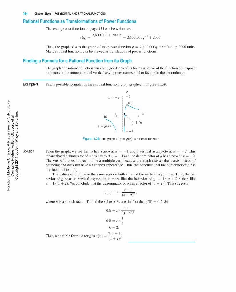
Proportionality and Power FunctionsThe following two examples introduce proportionality and power functions.

Example 1 The area, A, of a circle is proportional to the square of its radius, r:

A = πr2.

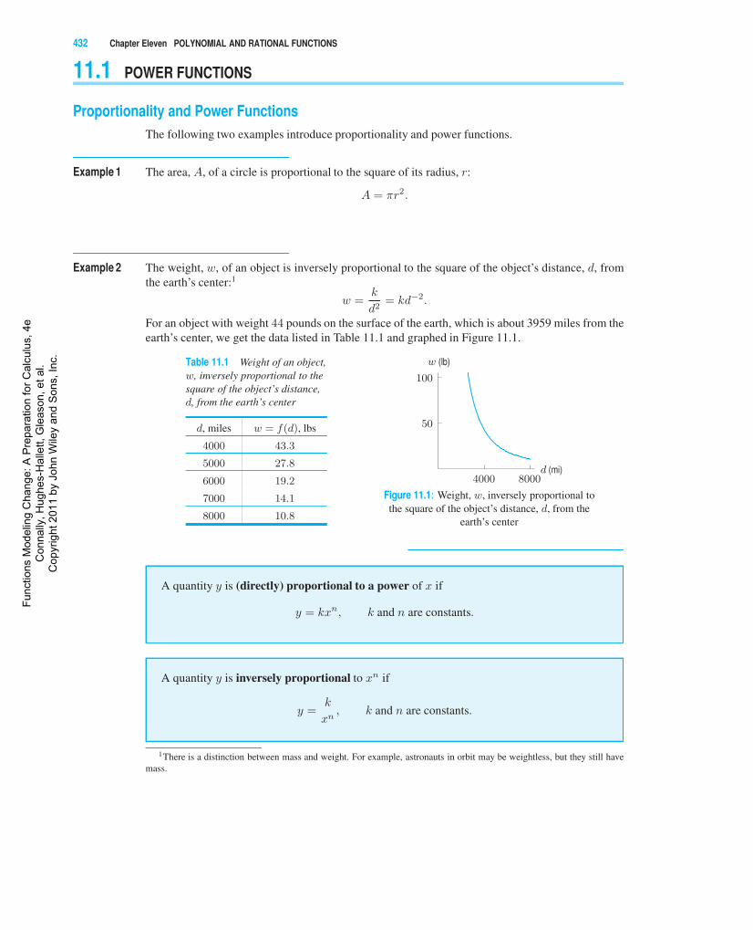
Example 2 The weight, w, of an object is inversely proportional to the square of the object’s distance, d, fromthe earth’s center:1

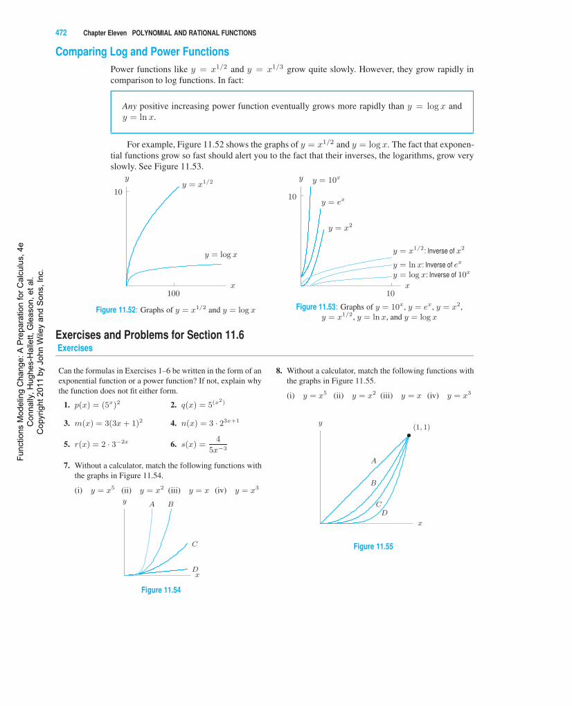
w =k

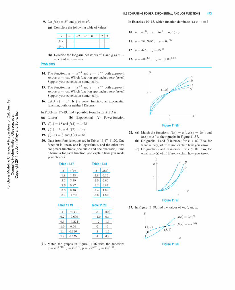
d2= kd−2.

For an object with weight 44 pounds on the surface of the earth, which is about 3959 miles from theearth’s center, we get the data listed in Table 11.1 and graphed in Figure 11.1.

Table 11.1 Weight of an object,w, inversely proportional to thesquare of the object’s distance,d, from the earth’s center

d, miles w = f(d), lbs

4000 43.3

5000 27.8

6000 19.2

7000 14.1

8000 10.8

4000 8000

50

100

d (mi)

w (lb)

Figure 11.1: Weight, w, inversely proportional tothe square of the object’s distance, d, from the

earth’s center

A quantity y is (directly) proportional to a power of x if

y = kxn, k and n are constants.

A quantity y is inversely proportional to xn if

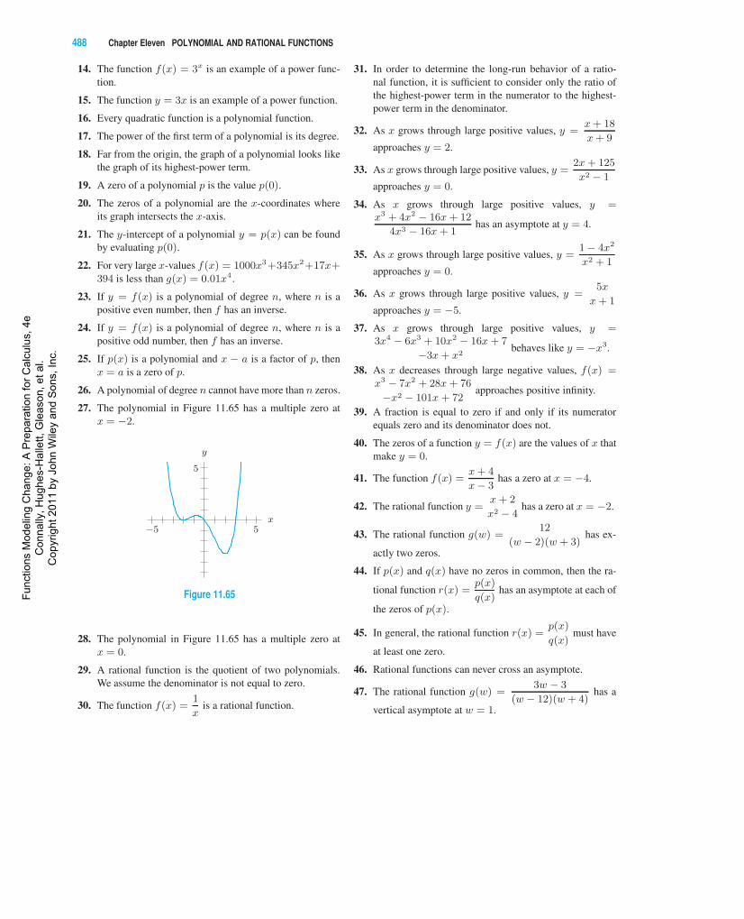
y =k

xn, k and n are constants.

1There is a distinction between mass and weight. For example, astronauts in orbit may be weightless, but they still havemass.

Func

tions

Mod

elin

g C

hang

e: A

Pre

para

tion

for C

alcu

lus,

4e

Con

nally

, Hug

hes-

Hal

lett,

Gle

ason

, et a

l. C

opyr

ight

201

1 by

Joh

n W

iley

and

Son

s, In

c.

11.1 POWER FUNCTIONS 433

The functions in Examples 1 and 2 are power functions. Generalizing, we define:

A power function is a function of the form

f(x) = kxp, where k and p are constants.

Example 3 Which of the following functions are power functions? For each power function, state the value ofthe constants k and p in the formula y = kxp.

(a) f(x) = 13 3√

x (b) g(x) = 2(x + 5)3 (c) u(x) =

√25

x3(d) v(x) = 6 · 3x

Solution The functions f and u are power functions; the functions g and v are not.

(a) The function f(x) = 13 3√

x is a power function because we can write its formula as

f(x) = 13x1/3.

Here, k = 13 and p = 1/3.(b) Although the value of g(x) = 2(x+5)3 is proportional to the cube of x+5, it is not proportional

to a power of x. We cannot write g(x) in the form g(x) = kxp; thus, g is not a power function.(c) We can rewrite the formula for u(x) =

√25/x3 as

u(x) =

√25√x3

=5

(x3)1/2=

5

x3/2= 5x−3/2.

Thus, u is a power function. Here, k = 5 and p = −3/2.(d) Although the value of v(x) = 6·3x is proportional to a power of 3, the power is not a constant—

it is the variable x. In fact, v(x) = 6 ·3x is an exponential function, not a power function. Noticethat y = 6 · x3 is a power function. However, 6 · x3 and 6 · 3x are quite different.

The Effect of the Power p

We now study functions whose constant of proportionality is k = 1 so that we can focus on theeffect of the power p.

Graphs of the Special Cases y = x0 and y = x

1

The power functions corresponding to p = 0 and p = 1 are both linear. The graph of y = x0 = 1 isa horizontal line through the point (1, 1). The graph of y = x1 = x is a line through the origin withslope +1.

(1, 1) y = x0 = 1

x

y

Figure 11.2: Graph of y = x0 = 1

(1, 1)

x

y = x1 = xy

Figure 11.3: Graph of y = x1 = x

Func

tions

Mod

elin

g C

hang

e: A

Pre

para

tion

for C

alcu

lus,

4e

Con

nally

, Hug

hes-

Hal

lett,

Gle

ason

, et a

l. C

opyr

ight

201

1 by

Joh

n W

iley

and

Son

s, In

c.


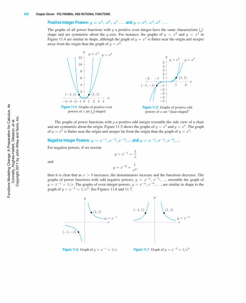
Positive Integer Powers: y = x3, x

5, x

7. . . and y = x

2, x

4, x

6. . .

The graphs of all power functions with p a positive even integer have the same characteristic⋃

-shape and are symmetric about the y-axis. For instance, the graphs of y = x2 and y = x4 inFigure 11.4 are similar in shape, although the graph of y = x4 is flatter near the origin and steeperaway from the origin than the graph of y = x2.

−4−3−2−1 0 1 2 3 4

2

4

6

8

10

12y = x2y = x4

(−1, 1) (1, 1)x

y

Figure 11.4: Graphs of positive evenpowers of x are

⋃-shaped

−2 −1

1 2

−5−4−3−2−1

12345

y = x3y = x5

(−1,−1)

(1, 1)x

y

Figure 11.5: Graphs of positive oddpowers of x are “chair-shaped”

The graphs of power functions with p a positive odd integer resemble the side view of a chairand are symmetric about the origin. Figure 11.5 shows the graphs of y = x3 and y = x5. The graphof y = x5 is flatter near the origin and steeper far from the origin than the graph of y = x3.

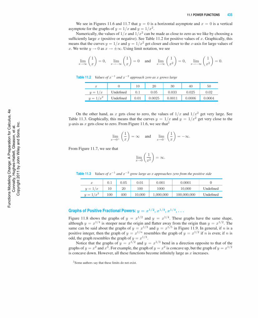
Negative Integer Powers: y = x−1, x

−3, x−5, ... and y = x

−2, x−4, x

−6, ...

For negative powers, if we rewrite

y = x−1 =1

x

and

y = x−2 =1

x2,

then it is clear that as x > 0 increases, the denominators increase and the functions decrease. Thegraphs of power functions with odd negative powers, y = x−3, x−5, . . ., resemble the graph ofy = x−1 = 1/x. The graphs of even integer powers, y = x−4, x−6, . . ., are similar in shape to thegraph of y = x−2 = 1/x2. See Figures 11.6 and 11.7.

x

y

(1, 1)

(−1,−1)

y = x−1

Figure 11.6: Graph of y = x−1 = 1/x

x

y

(1, 1)(−1, 1)

y = x−2

Figure 11.7: Graph of y = x−2 = 1/x2

Func

tions

Mod

elin

g C

hang

e: A

Pre

para

tion

for C

alcu

lus,

4e

Con

nally

, Hug

hes-

Hal

lett,

Gle

ason

, et a

l. C

opyr

ight

201

1 by

Joh

n W

iley

and

Son

s, In

c.


We see in Figures 11.6 and 11.7 that y = 0 is a horizontal asymptote and x = 0 is a verticalasymptote for the graphs of y = 1/x and y = 1/x2.

Numerically, the values of 1/x and 1/x2 can be made as close to zero as we like by choosing asufficiently large x (positive or negative). See Table 11.2 for positive values of x. Graphically, thismeans that the curves y = 1/x and y = 1/x2 get closer and closer to the x-axis for large values ofx. We write y → 0 as x→ ±∞. Using limit notation, we see

limx→∞

(1

x

)= 0, lim

x→−∞

(1

x

)= 0 and lim

x→∞

(1

x2

)= 0, lim

x→−∞

(1

x2

)= 0.

Table 11.2 Values of x−1 and x−2 approach zero as x grows large

x 0 10 20 30 40 50

y = 1/x Undefined 0.1 0.05 0.033 0.025 0.02

y = 1/x2 Undefined 0.01 0.0025 0.0011 0.0006 0.0004

On the other hand, as x gets close to zero, the values of 1/x and 1/x2 get very large. SeeTable 11.3. Graphically, this means that the curves y = 1/x and y = 1/x2 get very close to they-axis as x gets close to zero. From Figure 11.6, we see that2

limx→0+

(1

x

)=∞ and lim

x→0−

(1

x

)= −∞.

From Figure 11.7, we see that

limx→0

(1

x2

)= ∞.

Table 11.3 Values of x−1 and x−2 grow large as x approaches zero from the positive side

x 0.1 0.05 0.01 0.001 0.0001 0

y = 1/x 10 20 100 1000 10,000 Undefined

y = 1/x2 100 400 10,000 1,000,000 100,000,000 Undefined

Graphs of Positive Fractional Powers: y = x1/2, x

1/3, x1/4, . . .

Figure 11.8 shows the graphs of y = x1/2 and y = x1/4. These graphs have the same shape,although y = x1/4 is steeper near the origin and flatter away from the origin than y = x1/2. Thesame can be said about the graphs of y = x1/3 and y = x1/5 in Figure 11.9. In general, if n is apositive integer, then the graph of y = x1/n resembles the graph of y = x1/2 if n is even; if n isodd, the graph resembles the graph of y = x1/3.

Notice that the graphs of y = x1/2 and y = x1/3 bend in a direction opposite to that of thegraphs of y = x2 and x3. For example, the graph of y = x2 is concave up, but the graph of y = x1/2

is concave down. However, all these functions become infinitely large as x increases.

2Some authors say that these limits do not exist.

Func

tions

Mod

elin

g C

hang

e: A

Pre

para

tion

for C

alcu

lus,

4e

Con

nally

, Hug

hes-

Hal

lett,

Gle

ason

, et a

l. C

opyr

ight

201

1 by

Joh

n W

iley

and

Son

s, In

c.


−4 −3 −2 −1 1 2 3 4

−2

−1

1

2 y = x1/2

y = x1/4

(1, 1)

x

y

Figure 11.8: The graphs of y = x1/2 and y = x1/4

−4 −3 −2 −1 1 2 3 4

−2

11

2y = x1/3

y = x1/5

(−1,−1)

(1, 1)

x

y

Figure 11.9: The graphs of y = x1/3 and y = x1/5

Example 4 From geometry, we know that the radius of a sphere is directly proportional to the cube root of itsvolume. In this example, we use that proportionality relationship. If a sphere of radius 18.2 cm hasa volume of 25,252.4 cm3, what is the radius of a sphere whose volume is 30,000 cm3?

Solution Since the radius of the sphere is proportional to the cube root of its volume, we know that

r = kV 1/3, for k constant.

We also know that r = 18.2 cm when V = 25,252.4 cm3; therefore

18.2 = k(25,252.4)1/3,

giving

k =18.2

(25,252.4)1/3≈ 0.620.

Thus, when V = 30,000, we get r = 0.620(30,000)1/3 ≈ 19.3, so the radius of the sphere isapproximately 19.3 cm.

To compare the proportionality constant in Example 4 with that given by geometry, notice thatsince

V =4

3πr3,

we have

r =

(3

4πV

)1/3

=

(3

4π

)1/3

V 1/3.

Thus, the constant of proportionality is (3/(4π))1/3

= 0.620, as before.

Finding the Formula for a Power FunctionAs is the case for linear and exponential functions, the formula of a power function can be foundusing two points on its graph.

Func

tions

Mod

elin

g C

hang

e: A

Pre

para

tion

for C

alcu

lus,

4e

Con

nally

, Hug

hes-

Hal

lett,

Gle

ason

, et a

l. C

opyr

ight

201

1 by

Joh

n W

iley

and

Son

s, In

c.


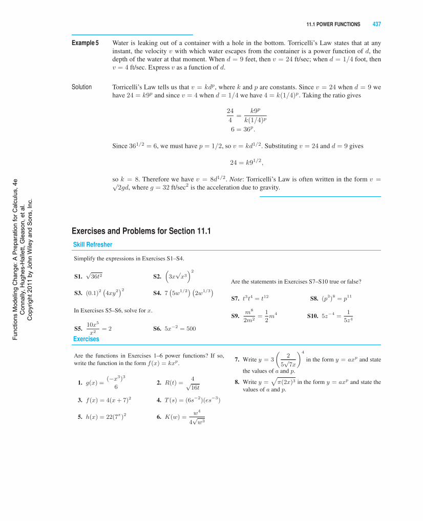
Example 5 Water is leaking out of a container with a hole in the bottom. Torricelli’s Law states that at anyinstant, the velocity v with which water escapes from the container is a power function of d, thedepth of the water at that moment. When d = 9 feet, then v = 24 ft/sec; when d = 1/4 foot, thenv = 4 ft/sec. Express v as a function of d.

Solution Torricelli’s Law tells us that v = kdp, where k and p are constants. Since v = 24 when d = 9 wehave 24 = k9p and since v = 4 when d = 1/4 we have 4 = k(1/4)p. Taking the ratio gives

24

4=

k9p

k(1/4)p

6 = 36p.

Since 361/2 = 6, we must have p = 1/2, so v = kd1/2. Substituting v = 24 and d = 9 gives

24 = k91/2,

so k = 8. Therefore we have v = 8d1/2. Note: Torricelli’s Law is often written in the form v =√2gd, where g = 32 ft/sec2 is the acceleration due to gravity.

Exercises and Problems for Section 11.1Skill Refresher

Simplify the expressions in Exercises S1–S4.

S1.√

36t2 S2.(3x√

x3

)2

S3. (0.1)2(4xy2

)2S4. 7

(5w1/2

) (2w1/3

)In Exercises S5–S6, solve for x.

S5.10x5

x2= 2 S6. 5x−2 = 500

Are the statements in Exercises S7–S10 true or false?

S7. t3t4 = t12 S8. (p3)8 = p11

S9.m8

2m2=

1

2m4 S10. 5z−4 =

1

5z4

Exercises

Are the functions in Exercises 1–6 power functions? If so,write the function in the form f(x) = kxp.

1. g(x) =(−x3)3

62. R(t) =

4√16t

3. f(x) = 4(x + 7)2 4. T (s) = (6s−2)(es−3)

5. h(x) = 22(7x)2 6. K(w) =w4

4√

w3

7. Write y = 3

(2

5√

7x

)4

in the form y = axp and state

the values of a and p.

8. Write y =√

π(2x)3 in the form y = axp and state thevalues of a and p.

Func

tions

Mod

elin

g C

hang

e: A

Pre

para

tion

for C

alcu

lus,

4e

Con

nally

, Hug

hes-

Hal

lett,

Gle

ason

, et a

l. C

opyr

ight

201

1 by

Joh

n W

iley

and

Son

s, In

c.


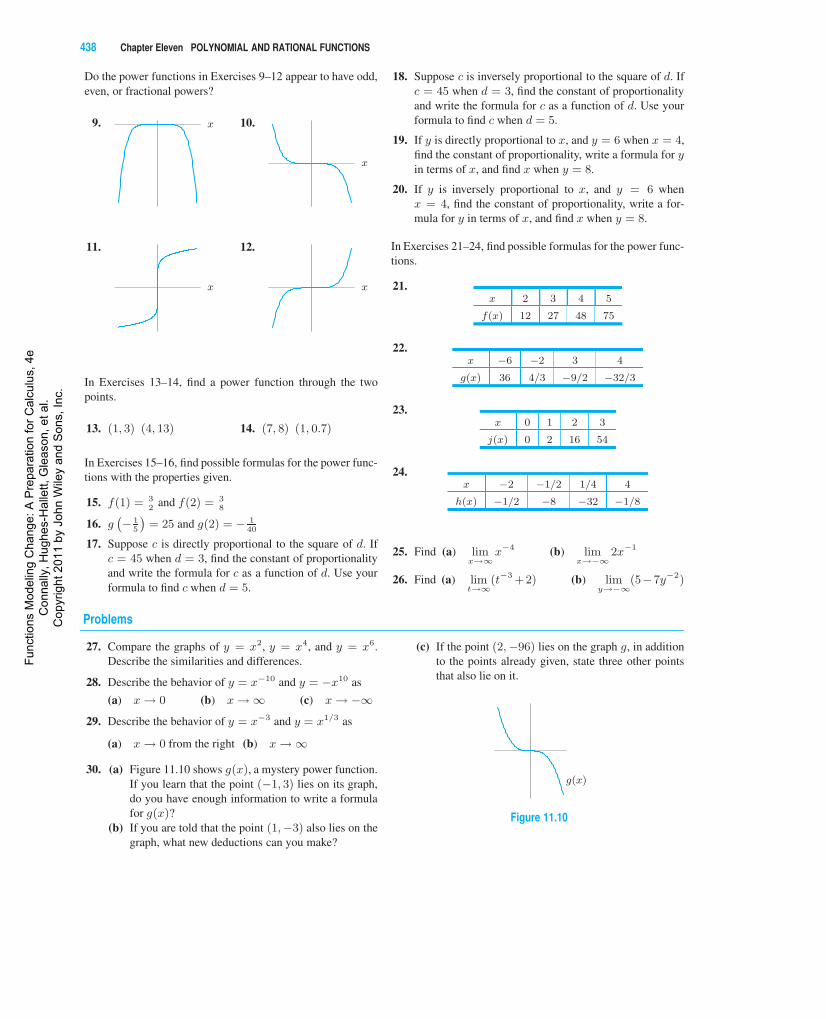
Do the power functions in Exercises 9–12 appear to have odd,even, or fractional powers?

9. x 10.

x

11.

x

12.

x

In Exercises 13–14, find a power function through the twopoints.

13. (1, 3) (4, 13) 14. (7, 8) (1, 0.7)

In Exercises 15–16, find possible formulas for the power func-tions with the properties given.

15. f(1) = 32

and f(2) = 38

16. g(− 1

5

)= 25 and g(2) = − 1

40

17. Suppose c is directly proportional to the square of d. Ifc = 45 when d = 3, find the constant of proportionalityand write the formula for c as a function of d. Use yourformula to find c when d = 5.

18. Suppose c is inversely proportional to the square of d. Ifc = 45 when d = 3, find the constant of proportionalityand write the formula for c as a function of d. Use yourformula to find c when d = 5.

19. If y is directly proportional to x, and y = 6 when x = 4,find the constant of proportionality, write a formula for yin terms of x, and find x when y = 8.

20. If y is inversely proportional to x, and y = 6 whenx = 4, find the constant of proportionality, write a for-mula for y in terms of x, and find x when y = 8.

In Exercises 21–24, find possible formulas for the power func-tions.

21.x 2 3 4 5

f(x) 12 27 48 75

22.x −6 −2 3 4

g(x) 36 4/3 −9/2 −32/3

23.x 0 1 2 3

j(x) 0 2 16 54

24.x −2 −1/2 1/4 4

h(x) −1/2 −8 −32 −1/8

25. Find (a) limx→∞

x−4 (b) limx→−∞

2x−1

26. Find (a) limt→∞

(t−3 +2) (b) limy→−∞

(5−7y−2)

Problems

27. Compare the graphs of y = x2, y = x4, and y = x6.Describe the similarities and differences.

28. Describe the behavior of y = x−10 and y = −x10 as

(a) x → 0 (b) x →∞ (c) x → −∞29. Describe the behavior of y = x−3 and y = x1/3 as

(a) x → 0 from the right (b) x →∞

30. (a) Figure 11.10 shows g(x), a mystery power function.If you learn that the point (−1, 3) lies on its graph,do you have enough information to write a formulafor g(x)?

(b) If you are told that the point (1,−3) also lies on thegraph, what new deductions can you make?

(c) If the point (2,−96) lies on the graph g, in additionto the points already given, state three other pointsthat also lie on it.

g(x)

Figure 11.10

Func

tions

Mod

elin

g C

hang

e: A

Pre

para

tion

for C

alcu

lus,

4e

Con

nally

, Hug

hes-

Hal

lett,

Gle

ason

, et a

l. C

opyr

ight

201

1 by

Joh

n W

iley

and

Son

s, In

c.


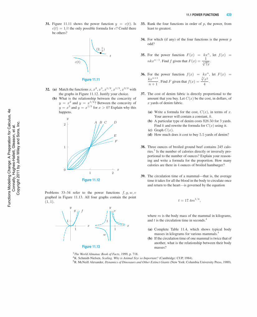
31. Figure 11.11 shows the power function y = c(t). Isc(t) = 1/t the only possible formula for c? Could therebe others?

(2, 12)

t

c(t)

Figure 11.11

32. (a) Match the functions x, x2, x3, x1/2, x1/3, x3/2 withthe graphs in Figure 11.12. Justify your choice.

(b) What is the relationship between the concavity ofy = x2 and y = x1/2? Between the concavity ofy = x3 and y = x1/3 for x > 0? Explain why thishappens.

1 20

1

2

x

y

F

E

C DBA

Figure 11.12

Problems 33–34 refer to the power functions f, g, w, vgraphed in Figure 11.13. All four graphs contain the point(1, 1).

1

1

fg

x

y

1

1

v

w

x

y

Figure 11.13

33. Rank the four functions in order of p, the power, fromleast to greatest.

34. For which (if any) of the four functions is the power podd?

35. For the power function F (x) = kxn, let f(x) =

nkxn−1. Find f given that F (x) =1

3√

7x.

36. For the power function f(x) = kxn, let F (x) =

kxn+1

n + 1. Find F given that f(x) =

5√

x2

4.

37. The cost of denim fabric is directly proportional to theamount that you buy. Let C(x) be the cost, in dollars, ofx yards of denim fabric.

(a) Write a formula for the cost, C(x), in terms of x.Your answer will contain a constant, k.

(b) A particular type of denim costs $28.50 for 3 yards.Find k and rewrite the formula for C(x) using it.

(c) Graph C(x).(d) How much does it cost to buy 5.5 yards of denim?

38. Three ounces of broiled ground beef contains 245 calo-ries.3 Is the number of calories directly or inversely pro-portional to the number of ounces? Explain your reason-ing and write a formula for the proportion. How manycalories are there in 4 ounces of broiled hamburger?

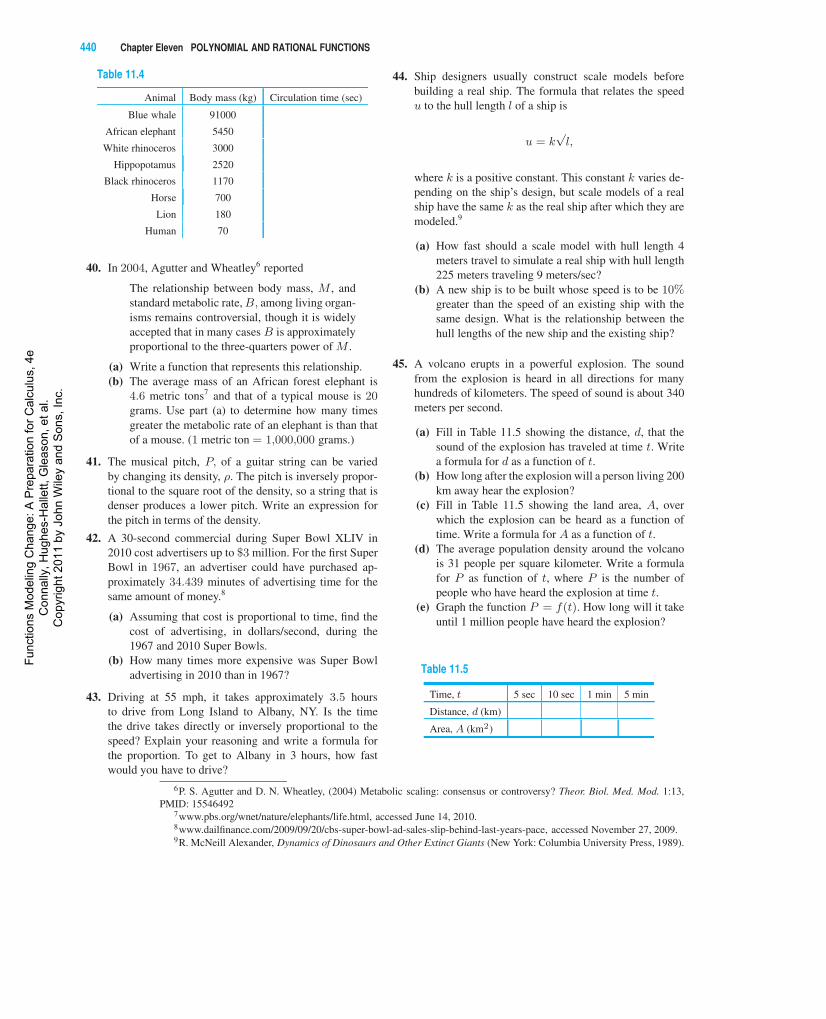
39. The circulation time of a mammal—that is, the averagetime it takes for all the blood in the body to circulate onceand return to the heart—is governed by the equation

t = 17.4m1/4,

where m is the body mass of the mammal in kilograms,and t is the circulation time in seconds.4

(a) Complete Table 11.4, which shows typical bodymasses in kilograms for various mammals.5

(b) If the circulation time of one mammal is twice that ofanother, what is the relationship between their bodymasses?

3The World Almanac Book of Facts, 1999, p. 718.4K. Schmidt-Nielsen, Scaling, Why is Animal Size so Important? (Cambridge: CUP, 1984).5R. McNeill Alexander, Dynamics of Dinosaurs and Other Extinct Giants (New York: Columbia University Press, 1989).

Func

tions

Mod

elin

g C

hang

e: A

Pre

para

tion

for C

alcu

lus,

4e

Con

nally

, Hug

hes-

Hal

lett,

Gle

ason

, et a

l. C

opyr

ight

201

1 by

Joh

n W

iley

and

Son

s, In

c.


Table 11.4

Animal Body mass (kg) Circulation time (sec)

Blue whale 91000

African elephant 5450

White rhinoceros 3000

Hippopotamus 2520

Black rhinoceros 1170

Horse 700

Lion 180

Human 70

40. In 2004, Agutter and Wheatley6 reported

The relationship between body mass, M , andstandard metabolic rate, B, among living organ-isms remains controversial, though it is widelyaccepted that in many cases B is approximatelyproportional to the three-quarters power of M .

(a) Write a function that represents this relationship.(b) The average mass of an African forest elephant is

4.6 metric tons7 and that of a typical mouse is 20grams. Use part (a) to determine how many timesgreater the metabolic rate of an elephant is than thatof a mouse. (1 metric ton = 1,000,000 grams.)

41. The musical pitch, P, of a guitar string can be variedby changing its density, ρ. The pitch is inversely propor-tional to the square root of the density, so a string that isdenser produces a lower pitch. Write an expression forthe pitch in terms of the density.

42. A 30-second commercial during Super Bowl XLIV in2010 cost advertisers up to $3 million. For the first SuperBowl in 1967, an advertiser could have purchased ap-proximately 34.439 minutes of advertising time for thesame amount of money.8

(a) Assuming that cost is proportional to time, find thecost of advertising, in dollars/second, during the1967 and 2010 Super Bowls.

(b) How many times more expensive was Super Bowladvertising in 2010 than in 1967?

43. Driving at 55 mph, it takes approximately 3.5 hoursto drive from Long Island to Albany, NY. Is the timethe drive takes directly or inversely proportional to thespeed? Explain your reasoning and write a formula forthe proportion. To get to Albany in 3 hours, how fastwould you have to drive?

44. Ship designers usually construct scale models beforebuilding a real ship. The formula that relates the speedu to the hull length l of a ship is

u = k√

l,

where k is a positive constant. This constant k varies de-pending on the ship’s design, but scale models of a realship have the same k as the real ship after which they aremodeled.9

(a) How fast should a scale model with hull length 4meters travel to simulate a real ship with hull length225 meters traveling 9 meters/sec?

(b) A new ship is to be built whose speed is to be 10%greater than the speed of an existing ship with thesame design. What is the relationship between thehull lengths of the new ship and the existing ship?

45. A volcano erupts in a powerful explosion. The soundfrom the explosion is heard in all directions for manyhundreds of kilometers. The speed of sound is about 340meters per second.

(a) Fill in Table 11.5 showing the distance, d, that thesound of the explosion has traveled at time t. Writea formula for d as a function of t.

(b) How long after the explosion will a person living 200km away hear the explosion?

(c) Fill in Table 11.5 showing the land area, A, overwhich the explosion can be heard as a function oftime. Write a formula for A as a function of t.

(d) The average population density around the volcanois 31 people per square kilometer. Write a formulafor P as function of t, where P is the number ofpeople who have heard the explosion at time t.

(e) Graph the function P = f(t). How long will it takeuntil 1 million people have heard the explosion?

Table 11.5

Time, t 5 sec 10 sec 1 min 5 min

Distance, d (km)

Area, A (km2)

6P. S. Agutter and D. N. Wheatley, (2004) Metabolic scaling: consensus or controversy? Theor. Biol. Med. Mod. 1:13,PMID: 15546492

7www.pbs.org/wnet/nature/elephants/life.html, accessed June 14, 2010.8www.dailfinance.com/2009/09/20/cbs-super-bowl-ad-sales-slip-behind-last-years-pace, accessed November 27, 2009.9R. McNeill Alexander, Dynamics of Dinosaurs and Other Extinct Giants (New York: Columbia University Press, 1989).

Func

tions

Mod

elin

g C

hang

e: A

Pre

para

tion

for C

alcu

lus,

4e

Con

nally

, Hug

hes-

Hal

lett,

Gle

ason

, et a

l. C

opyr

ight

201

1 by

Joh

n W

iley

and

Son

s, In

c.

11.2 POLYNOMIAL FUNCTIONS 441

46. Two oil tankers crash in the Pacific Ocean. The spreadingoil slick has a circular shape, and the radius of the circleis increasing at 200 meters per hour.

(a) Express the radius of the spill, r, as a power functionof time, t, in hours since the crash.

(b) Express the area of the spill, A, as a power functionof time, t.

(c) Clean-up efforts begin 7 hours after the spill. Howlarge an area is covered by oil at that time?

47. In a microwave oven, cooking time is inversely propor-tional to the amount of power used. It takes 6.5 minutesto heat a frozen dinner at 750 watts.

(a) Write a formula for the cooking time, t, as a functionof power level, w.

(b) Fill in Table 11.6 with the cooking times needed toheat the frozen dinner at various power levels.

(c) Graph the function t = f(w).(d) If it takes 2 minutes to heat a rhubarb crumble at 250

watts, how long will it take at 500 watts?

Table 11.6

Power, w (watts) 250 300 500 650

Time, t (mins)

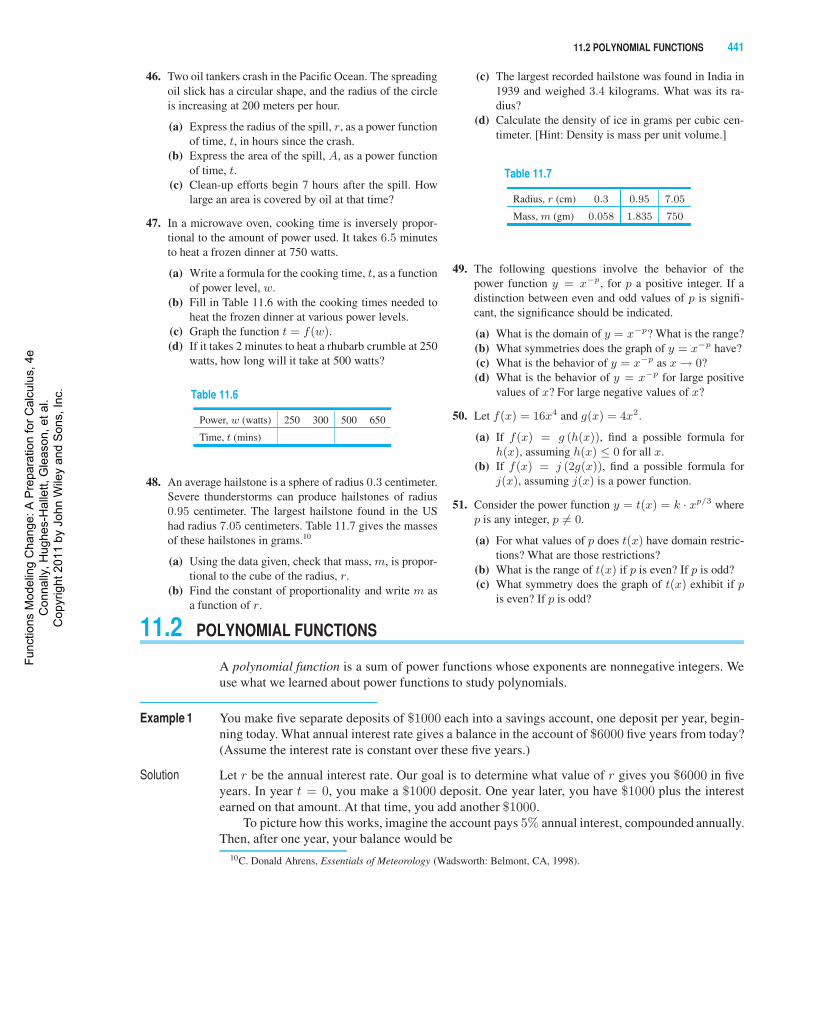
48. An average hailstone is a sphere of radius 0.3 centimeter.Severe thunderstorms can produce hailstones of radius0.95 centimeter. The largest hailstone found in the UShad radius 7.05 centimeters. Table 11.7 gives the massesof these hailstones in grams.10

(a) Using the data given, check that mass, m, is propor-tional to the cube of the radius, r.

(b) Find the constant of proportionality and write m asa function of r.

(c) The largest recorded hailstone was found in India in1939 and weighed 3.4 kilograms. What was its ra-dius?

(d) Calculate the density of ice in grams per cubic cen-timeter. [Hint: Density is mass per unit volume.]

Table 11.7

Radius, r (cm) 0.3 0.95 7.05

Mass, m (gm) 0.058 1.835 750

49. The following questions involve the behavior of thepower function y = x−p, for p a positive integer. If adistinction between even and odd values of p is signifi-cant, the significance should be indicated.

(a) What is the domain of y = x−p? What is the range?(b) What symmetries does the graph of y = x−p have?(c) What is the behavior of y = x−p as x → 0?(d) What is the behavior of y = x−p for large positive

values of x? For large negative values of x?

50. Let f(x) = 16x4 and g(x) = 4x2.

(a) If f(x) = g (h(x)), find a possible formula forh(x), assuming h(x) ≤ 0 for all x.

(b) If f(x) = j (2g(x)), find a possible formula forj(x), assuming j(x) is a power function.

51. Consider the power function y = t(x) = k · xp/3 wherep is any integer, p �= 0.

(a) For what values of p does t(x) have domain restric-tions? What are those restrictions?

(b) What is the range of t(x) if p is even? If p is odd?(c) What symmetry does the graph of t(x) exhibit if p

is even? If p is odd?

11.2 POLYNOMIAL FUNCTIONS

A polynomial function is a sum of power functions whose exponents are nonnegative integers. Weuse what we learned about power functions to study polynomials.

Example 1 You make five separate deposits of $1000 each into a savings account, one deposit per year, begin-ning today. What annual interest rate gives a balance in the account of $6000 five years from today?(Assume the interest rate is constant over these five years.)

Solution Let r be the annual interest rate. Our goal is to determine what value of r gives you $6000 in fiveyears. In year t = 0, you make a $1000 deposit. One year later, you have $1000 plus the interestearned on that amount. At that time, you add another $1000.

To picture how this works, imagine the account pays 5% annual interest, compounded annually.Then, after one year, your balance would be

10C. Donald Ahrens, Essentials of Meteorology (Wadsworth: Belmont, CA, 1998).

Func

tions

Mod

elin

g C

hang

e: A

Pre

para

tion

for C

alcu

lus,

4e

Con

nally

, Hug

hes-

Hal

lett,

Gle

ason

, et a

l. C

opyr

ight

201

1 by

Joh

n W

iley

and

Son

s, In

c.


Balance = (100% of Initial deposit) + (5% of Initial deposit) + Second deposit

= 105% of Initial deposit︸︷︷︸$1000

+ Second deposit︸︷︷︸$1000

= 1.05(1000) + 1000.

Let x represent the annual growth factor, 1 + r. For example, if the account paid 5% interest, thenx = 1 + 0.05 = 1.05. We write the balance after one year in terms of x:

Balance after one year = 1000x + 1000.

After two years, you would have earned interest on the first-year balance. This gives

Balance after earning interest = (1000x + 1000︸︷︷︸First-year balance

)x = 1000x2 + 1000x.

The third $1000 deposit brings your balance to

Balance after two years = 1000x2 + 1000x + 1000.︸︷︷︸Third deposit

A year’s worth of interest on this amount, plus the fourth $1000 deposit, brings your balance to

Balance after three years = (1000x2 + 1000x + 1000︸︷︷︸Second-year balance

)x + 1000︸︷︷︸Fourth deposit

= 1000x3 + 1000x2 + 1000x + 1000.

The pattern is this: Each of the $1000 deposits grows to $1000xn by the end of its nth year in thebank. Thus,

Balance after five years = 1000x5 + 1000x4 + 1000x3 + 1000x2 + 1000x.

If the interest rate is chosen correctly, then the balance will be $6000 in five years. This gives us

1000x5 + 1000x4 + 1000x3 + 1000x2 + 1000x = 6000.

Dividing by 1000 and moving the 6 to the left side, we have the equation

x5 + x4 + x3 + x2 + x− 6 = 0.

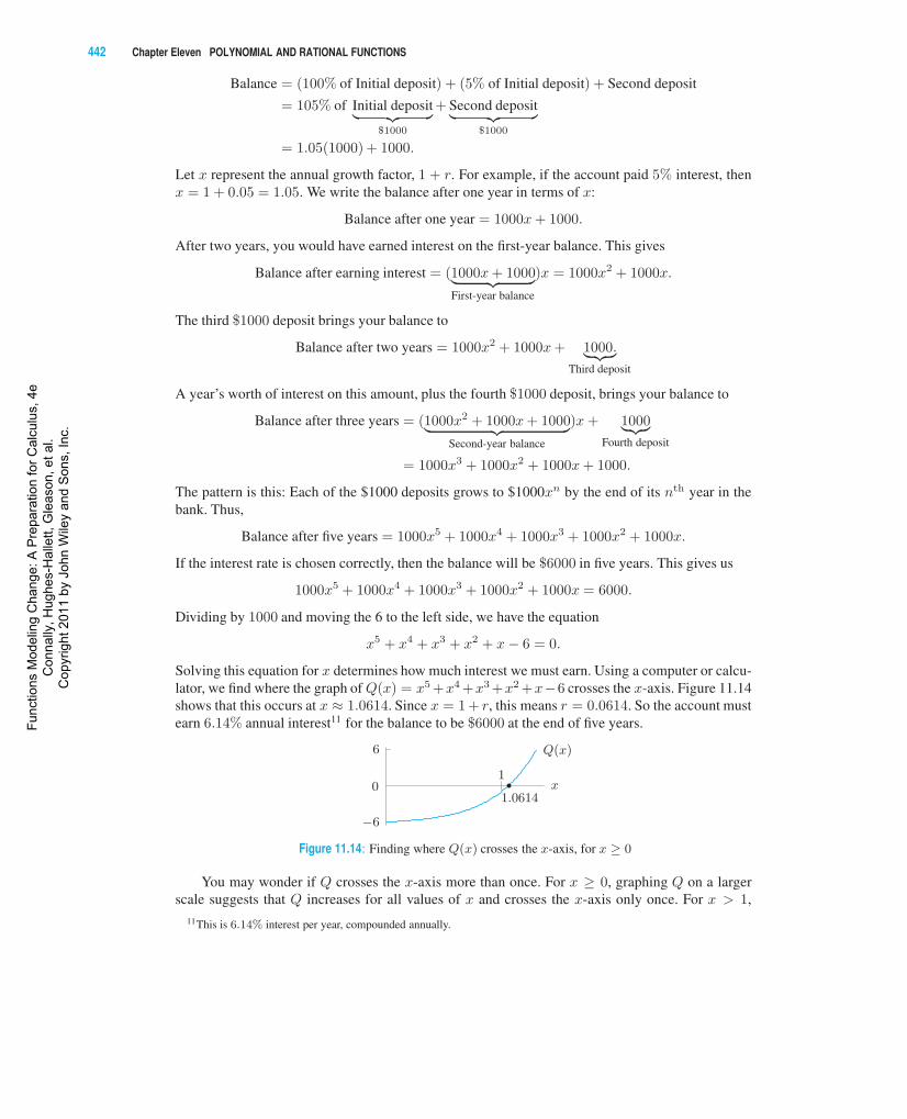
Solving this equation for x determines how much interest we must earn. Using a computer or calcu-lator, we find where the graph of Q(x) = x5 +x4 +x3 +x2 +x−6 crosses the x-axis. Figure 11.14shows that this occurs at x ≈ 1.0614. Since x = 1 + r, this means r = 0.0614. So the account mustearn 6.14% annual interest11 for the balance to be $6000 at the end of five years.

1

1.0614

−6

6

x0

Q(x)

Figure 11.14: Finding where Q(x) crosses the x-axis, for x ≥ 0

You may wonder if Q crosses the x-axis more than once. For x ≥ 0, graphing Q on a largerscale suggests that Q increases for all values of x and crosses the x-axis only once. For x > 1,

11This is 6.14% interest per year, compounded annually.

Func

tions

Mod

elin

g C

hang

e: A

Pre

para

tion

for C

alcu

lus,

4e

Con

nally

, Hug

hes-

Hal

lett,

Gle

ason

, et a

l. C

opyr

ight

201

1 by

Joh

n W

iley

and

Son

s, In

c.


we expect Q to be an increasing function, because larger values of x indicate higher interest ratesand therefore larger values of Q(x). Having crossed the axis once, the graph of Q does not “turnaround” to cross it again.

The function Q(x) = x5 + x4 + x3 + x2 + x− 6 is the sum of power functions; Q is called apolynomial. (Note that the expression −6 can be written as −6x0, so it, too, is a power function.)

A General Formula for the Family of Polynomial FunctionsThe general formula for a polynomial function can be written as

p(x) = anxn + an−1xn−1 + ... + a1x + a0,

where n is called the degree of the polynomial and an is the leading coefficient. For example, thefunction

g(x) = 3x2 + 4x5 + x− x3 + 1,

is a polynomial of degree 5 because the term with the highest power is 4x5. It is customary to writea polynomial with the powers in decreasing order from left to right:

g(x) = 4x5 − x3 + 3x2 + x + 1.

The function g has one other term, 0 · x4, which we don’t bother to write down. The values of g’scoefficients are a5 = 4, a4 = 0, a3 = −1, a2 = 3, a1 = 1, and a0 = 1. In summary:

The general formula for the family of polynomial functions can be written as

p(x) = anxn + an−1xn−1 + . . . + a1x + a0,

where n is a positive integer called the degree of p and where an �= 0.• Each power function aix

i in this sum is called a term.

• The constants an, an−1, . . . , a0 are called coefficients.

• The term a0 is called the constant term. The term with the highest power, anxn, is calledthe leading term.

• To write a polynomial in standard form, we arrange its terms from highest power tolowest power, going from left to right.

Like the power functions from which they are built, polynomials are defined for all valuesof x. Except for polynomials of degree zero (whose graphs are horizontal lines), the graphs ofpolynomials do not have horizontal or vertical asymptotes; they are smooth and unbroken. Theshape of the graph depends on its degree; typical graphs are shown in Figure 11.15.

Quadratic(n = 2)

Cubic(n = 3)

Quartic(n = 4)

Quintic(n = 5)

Figure 11.15: Graphs of typical polynomials of degree n

Func

tions

Mod

elin

g C

hang

e: A

Pre

para

tion

for C

alcu

lus,

4e

Con

nally

, Hug

hes-

Hal

lett,

Gle

ason

, et a

l. C

opyr

ight

201

1 by

Joh

n W

iley

and

Son

s, In

c.


The Long-Run Behavior of Polynomial FunctionsWe have seen that, as x grows large, y = x2 increases fast, y = x3 increases faster, and y = x4

increases faster still. In general, power functions with larger positive powers eventually grow muchfaster than those with smaller powers. This tells us about the behavior of polynomials for large x.For instance, consider the polynomial g(x) = 4x5 − x3 + 3x2 + x + 1. Provided x is large enough,the value of the term 4x5 is much larger than the value of the other terms combined. For example,if x = 100,

4x5 = 4(100)5 = 40,000,000,000,

and the other terms in g(x) are

−x3 + 3x2 + x + 1 = −(100)3 + 3(100)2 + 100 + 1

= −1,000,000 + 30,000 + 100 + 1 = −969,899.

Therefore p(100) = 39,999,030,101, which is approximately equal to the value of the 4x5 term. Ingeneral, if x is large enough, the most important contribution to the value of a polynomial p is madeby the leading term; we can ignore the lower power terms.

When viewed on a large enough scale, the graph of the polynomial p(x) = anxn +an−1x

n−1 + · · · + a1x + a0 looks like the graph of the power function y = anxn. Thisbehavior is called the long-run behavior of the polynomial. Using limit notation, we write

limx→∞

p(x) = limx→∞

anxn and limx→−∞

p(x) = limx→−∞

anxn.

Example 2 Find a window in which the graph of f(x) = x3 + x2 resembles the power function y = x3.

Solution Figure 11.16 gives the graphs of f(x) = x3 + x2 and y = x3. On this scale, f does not look like apower function. On the larger scale in Figure 11.17, the graph of f resembles the graph of y = x3.On this larger scale, the “bumps” in the graph of f are too small to be seen. On an even larger scale,as in Figure 11.18, the graph of f is indistinguishable from the graph of y = x3.

−2 2

−1

1

f(x)

x

y

x3

�Bump

�Bump

Figure 11.16: On this scale,f(x) = x3 + x2 does not look

like a power function

−5 5

−150

150 f(x)

x

y

x3

�

Bump nolonger visible

Figure 11.17: On this scale,f(x) = x3 + x2 resembles the

power function y = x3

−10 10

−1000

1000 f(x)

x

y

x3

Figure 11.18: On this scale,f(x) = x3 + x2 is nearly

indistinguishable from y = x3

Zeros of PolynomialsThe zeros of a polynomial p are values of x for which p(x) = 0. The zeros are also the x-intercepts,because they tell us where the graph of p crosses the x-axis. Factoring can sometimes be used tofind the zeros of a polynomial; however, the graphical method of Example 1 can always be used. Inaddition, the long-run behavior of the polynomial can give us clues as to how many zeros (if any)there may be.

Func

tions

Mod

elin

g C

hang

e: A

Pre

para

tion

for C

alcu

lus,

4e

Con

nally

, Hug

hes-

Hal

lett,

Gle

ason

, et a

l. C

opyr

ight

201

1 by

Joh

n W

iley

and

Son

s, In

c.


Example 3 Given the polynomialq(x) = 3x6 − 2x5 + 4x2 − 1,

where q(0) = −1, is there a reason to expect a solution to the equation q(x) = 0? If not, explainwhy not. If so, how do you know?

Solution The equation q(x) = 0 must have at least two solutions. We know this because on a large scale, qlooks like the power function y = 3x6. (See Figure 11.19.) The function y = 3x6 takes on largepositive values as x grows large (either positive or negative). Since the graph of q is smooth andunbroken, it must cross the x-axis at least twice to get from q(0) = −1 to the positive values itattains as x →∞ and x → −∞.

−1.5 1.5−10

50

q(x) = 3x6 − 2x5 + 4x2 − 1

x

Figure 11.19: Graph must cross x-axis at least twice since q(0) = −1 and q(x) looks like 3x6 for large x

A sixth-degree polynomial such as q in Example 3 can have as many as six real zeros. Weconsider the zeros of a polynomial in more detail in Section 11.3.

Exercises and Problems for Section 11.2Exercises

Are the functions in Exercises 1–6 polynomials? If so, of whatdegree?

1. y = 5x − 2 2. y = 5 + x

3. y = 4x2 + 2 4. y = 7t6 − 8t + 7.2

5. y = 4x4 − 3x3 + 2ex 6. y = 4x2 − 7√

x9 + 10

For the polynomials in Exercises 7–9, state the degree, thenumber of terms, and describe the long-run behavior.

7. y = 2x3 − 3x + 7

8. y = 1− 2x4 + x3

9. y = (x + 4)(2x − 3)(5− x)

10. Find

(a) limx→∞

(3x2 − 5x + 7) (b) limx→−∞

(7x2 − 9x3)

Problems

11. Estimate the zeros of f(x) = x4 − 3x2 − x + 2.

12. Estimate the minimum value of g(x) = x4 − 3x3 − 8.

13. Compare the graphs of f(x) = x3 + 5x2 − x − 5 andg(x) = −2x3 − 10x2 + 2x + 10 on a window thatshows all intercepts. How are the graphs similar? Dif-ferent? Discuss.

14. Let u(x) = − 15(x− 3)(x + 1)(x + 5)

and v(x) = − 15x2(x− 5).

(a) Graph u and v for −10 ≤ x ≤ 10, −10 ≤ y ≤ 10.How are the graphs similar? How are they different?

(b) Compare the graphs of u and v on the window−20 ≤ x ≤ 20, −1600 ≤ y ≤ 1600, the win-dow −50 ≤ x ≤ 50, −25,000 ≤ y ≤ 25,000,and the window −500 ≤ x ≤ 500, −25,000,000 ≤y ≤ 25,000,000. Discuss.

Func

tions

Mod

elin

g C

hang

e: A

Pre

para

tion

for C

alcu

lus,

4e

Con

nally

, Hug

hes-

Hal

lett,

Gle

ason

, et a

l. C

opyr

ight

201

1 by

Joh

n W

iley

and

Son

s, In

c.


15. Find the equation of the line through the y-intercept ofy = x4−3x5−1+x2 and the x-intercept of y = 2x−4.

16. Let f(x) =

(1

50,000

)x3 +

(1

2

)x.

(a) For small values of x, which term of f is more im-portant? Explain your answer.

(b) Graph y = f(x) for −10 ≤ x ≤ 10, −10 ≤ y ≤10. Is this graph linear? How does the appearance ofthis graph agree with your answer to part (a)?

(c) How large a value of x is required for the cubic termof f to be equal to the linear term?

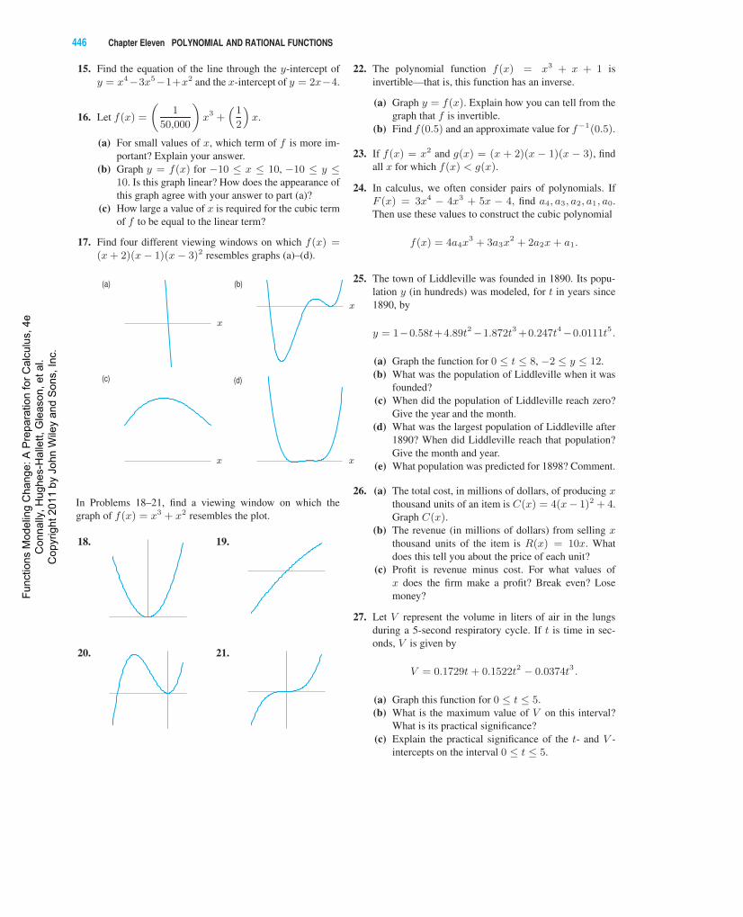
17. Find four different viewing windows on which f(x) =(x + 2)(x− 1)(x− 3)2 resembles graphs (a)–(d).

x

(a)

x

(b)

x

(c)

x

(d)

In Problems 18–21, find a viewing window on which thegraph of f(x) = x3 + x2 resembles the plot.

18. 19.

20. 21.

22. The polynomial function f(x) = x3 + x + 1 isinvertible—that is, this function has an inverse.

(a) Graph y = f(x). Explain how you can tell from thegraph that f is invertible.

(b) Find f(0.5) and an approximate value for f−1(0.5).

23. If f(x) = x2 and g(x) = (x + 2)(x − 1)(x − 3), findall x for which f(x) < g(x).

24. In calculus, we often consider pairs of polynomials. IfF (x) = 3x4 − 4x3 + 5x − 4, find a4, a3, a2, a1, a0.Then use these values to construct the cubic polynomial

f(x) = 4a4x3 + 3a3x

2 + 2a2x + a1.

25. The town of Liddleville was founded in 1890. Its popu-lation y (in hundreds) was modeled, for t in years since1890, by

y = 1−0.58t+4.89t2−1.872t3 +0.247t4−0.0111t5.

(a) Graph the function for 0 ≤ t ≤ 8, −2 ≤ y ≤ 12.(b) What was the population of Liddleville when it was

founded?(c) When did the population of Liddleville reach zero?

Give the year and the month.(d) What was the largest population of Liddleville after

1890? When did Liddleville reach that population?Give the month and year.

(e) What population was predicted for 1898? Comment.

26. (a) The total cost, in millions of dollars, of producing xthousand units of an item is C(x) = 4(x− 1)2 + 4.Graph C(x).

(b) The revenue (in millions of dollars) from selling xthousand units of the item is R(x) = 10x. Whatdoes this tell you about the price of each unit?

(c) Profit is revenue minus cost. For what values ofx does the firm make a profit? Break even? Losemoney?

27. Let V represent the volume in liters of air in the lungsduring a 5-second respiratory cycle. If t is time in sec-onds, V is given by

V = 0.1729t + 0.1522t2 − 0.0374t3 .

(a) Graph this function for 0 ≤ t ≤ 5.(b) What is the maximum value of V on this interval?

What is its practical significance?(c) Explain the practical significance of the t- and V -

intercepts on the interval 0 ≤ t ≤ 5.

Func

tions

Mod

elin

g C

hang

e: A

Pre

para

tion

for C

alcu

lus,

4e

Con

nally

, Hug

hes-

Hal

lett,

Gle

ason

, et a

l. C

opyr

ight

201

1 by

Joh

n W

iley

and

Son

s, In

c.

11.3 THE SHORT-RUN BEHAVIOR OF POLYNOMIALS 447

28. The volume, V , in milliliters, of 1 kg of water as a func-tion of temperature T is given, for 0 ≤ T ≤ 30◦C, by:

V = 999.87−0.06426T+0.0085143T 2−0.0000679T 3 .

(a) Graph V .(b) Describe the shape of your graph. Does V increase

or decrease as T increases? Does the graph curveupward or downward? What does the graph tell usabout how the volume varies with temperature?

(c) At what temperature does water have the maxi-mum density? How does that appear on your graph?(Density = Mass/Volume. In this problem, the massof the water is 1 kg.)

29. Let f and g be polynomial functions. Are the followingcompositions also polynomial functions? Explain youranswer.

f(g(x)) and g(f(x))

30. (a) Suppose f(x) = ax2 + bx + c. What must be trueabout the coefficients if f is an even function?

(b) Suppose g(x) = ax3 + bx2 + cx+d. What must betrue about the coefficients if g is an odd function?

31. Let g be a polynomial function of degree n, where n isa positive odd integer. For each of the following state-ments, write true if the statement is always true, falseotherwise. If the statement is false, give an example thatillustrates why it is false.

(a) g is an odd function.(b) g has an inverse.(c) lim

x→∞g(x) =∞.

(d) If limx→−∞

g(x) = −∞, then limx→∞

g(x) =∞.

32. Let f(x) = x− x3

6+

x5

120.

(a) Graph y = f(x) and y = sin x for −2π ≤ x ≤ 2π,−3 ≤ y ≤ 3.

(b) The graph of f resembles the graph of sin x on asmall interval. Based on your graphs from part (a),give the approximate interval.

(c) Your calculator uses a function similar to f in or-der to evaluate the sine function. How reasonable anapproximation does f give for sin(π/8)?

(d) Explain how you could use the function f to ap-proximate the value of sin θ, where θ = 18 radians.[Hint: Use the fact that the sine function is periodic.]

33. For certain x-values, the function f(x) = 1/(1 + x) canbe well-approximated by the polynomial

p(x) = 1− x + x2 − x3 + x4 − x5.

(a) Show that p(0.5) ≈ f(0.5) = 2/3. To how manydecimal places do p(0.5) and f(0.5) agree?

(b) Calculate p(1). How well does p(1) approximatef(1)?

(c) Graph p(x) and f(x) together on the same set ofaxes for −1 ≤ x ≤ 1. Based on your graph, forwhat range of values of x does p(x) appear to give agood estimate for f(x)?

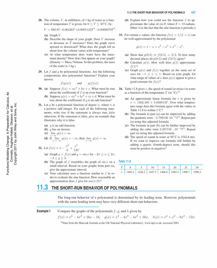
34. Table 11.8 gives v, the speed of sound (in m/sec) in wateras a function of the temperature T (in ◦C).12

(a) An approximate linear formula for v is given byv = 1402.385 + 5.038813T . Over what tempera-ture range does this formula agree with the values inTable 11.8 to within 1◦C?

(b) The formula in part (a) can be improved by addingthe quadratic term−5.799136·10−2T 2. Repeat part(a) using this adjusted formula.

(c) The formula in part (b) can be further improved byadding the cubic term 3.287156 · 10−4T 3. Repeatpart (a) using this adjusted formula.

(d) The speed of sound in water at 50◦C is 1542.6 m/s.If we want to improve our formula still further byadding a quartic (fourth-degree) term, should thisterm be positive or negative?

Table 11.8

T 0 5 10 15 20 25 30

v 1402.4 1426.2 1447.3 1466.0 1482.4 1496.7 1509.2

11.3 THE SHORT-RUN BEHAVIOR OF POLYNOMIALS

The long-run behavior of a polynomial is determined by its leading term. However, polynomialswith the same leading term may have very different short-run behaviors.

Example 1 Compare the graphs of the polynomials f , g, and h given by

f(x) = x4 − 4x3 + 16x− 16, g(x) = x4 − 4x3 − 4x2 + 16x, h(x) = x4 + x3 − 8x2 − 12x.

12Data from the Marczak formula at the UK National Physical Laboratory: www.npl.co.uk, accessed 2001.

Func

tions

Mod

elin

g C

hang

e: A

Pre

para

tion

for C

alcu

lus,

4e

Con

nally

, Hug

hes-

Hal

lett,

Gle

ason

, et a

l. C

opyr

ight

201

1 by

Joh

n W

iley

and

Son

s, In

c.


Solution Each of these functions is a fourth-degree polynomial, and each has x4 as its leading term. Thus, alltheir graphs resemble the graph of x4 on a large scale. See Figure 11.20.

However, on a smaller scale, the functions look different. See Figure 11.21. Two of the graphsgo through the origin while the third does not. The graphs also differ from one another in the numberof bumps each one has and in the number of times each one crosses the x-axis. Thus, polynomialswith the same leading term look similar on a large scale, but may look dissimilar on a small scale.

−8 8

4000

x

f(x)g(x)

h(x)

−8 8

4000

x

x4

Figure 11.20: On a large scale, the polynomials f , g, and h resemble the power function y = x4

−5 5

−35

15

x

f(x)

−5 5

−35

15

x

g(x)

−5 5

−35

15

x

h(x)

Figure 11.21: On a smaller scale, the polynomials f , g, and h look quite different from one another

Factored Form, Zeros, and the Short-Run Behavior of a PolynomialTo predict the long-run behavior of a polynomial, we use the highest-power term. To determine thezeros and the short-run behavior of a polynomial, we write it in factored form with as many linearfactors as possible.

Example 2 Investigate the short-run behavior of the third-degree polynomial u(x) = x3 − x2 − 6x.

(a) Rewrite u(x) as a product of linear factors.(b) Find the zeros of u(x).(c) Describe the graph of u(x). Where does it cross the x-axis? the y-axis? Where is u(x) positive?

Negative?

Solution (a) By factoring out an x and then factoring the quadratic, x2 − x− 6, we rewrite u(x) as

u(x) = x3 − x2 − 6x = x(x2 − x− 6) = x(x− 3)(x + 2).

Thus, we have expressed u(x) as the product of three linear factors, x, x− 3, and x + 2.(b) The polynomial equals zero if and only if at least one of its factors is zero. We solve the equation:

x(x − 3)(x + 2) = 0,

givingx = 0, or x− 3 = 0, or x + 2 = 0,

sox = 0, or x = 3, or x = −2.

These are the zeros, or x-intercepts, of u. To check, evaluate u(x) for these x-values; you shouldget 0. There are no other zeros.

Func

tions

Mod

elin

g C

hang

e: A

Pre

para

tion

for C

alcu

lus,

4e

Con

nally

, Hug

hes-

Hal

lett,

Gle

ason

, et a

l. C

opyr

ight

201

1 by

Joh

n W

iley

and

Son

s, In

c.


(c) To describe the graph of u, we give the x- and y-intercepts, and the long-run behavior.The factored form, u(x) = x(x − 3)(x + 2), shows that the graph crosses the x-axis at

x = 0, 3,−2. The graph of u crosses the y-axis at u(0) = 03− 02− 6 · 0 = 0; that is, at y = 0.For large values of x, the graph of y = u(x) resembles the graph of its leading term, y = x3.Figure 11.22 shows where u is positive and where u is negative.

−5−4−3−2−1 1 2 3 4 5

−20

−10

10

20

x

y

y = x3 y = u(x)

� u positive�

u positive

�

u negative

�u negative

Figure 11.22: The graph of u(x) = x3 − x2 − 6x has zeros atx = −2, 0, and 3. Its long-run behavior resembles y = x3

In Example 2, each linear factor produced a zero of the polynomial. Now suppose that we donot know the polynomial p, but we do know that it has zeros at x = 0, −12, 31. Then we knowthat the factored form of the polynomial must include the factors (x − 0) or x, and (x− (−12)) or(x + 12), and (x− 31). It may include other factors too. In summary:

Suppose p is a polynomial. If the formula for p has a linear factor, that is, a factor of theform (x− k), then p has a zero at x = k.Conversely, if p has a zero at x = k, then p has a linear factor of the form (x− k).

The Number of Factors, Zeros, and Bumps

The number of linear factors is always less than or equal to the degree of a polynomial. For example,a fourth-degree polynomial can have no more than four linear factors. This makes sense because ifwe had another factor in the product and multiplied out, the highest power of x would be greaterthan four. Since each zero corresponds to a linear factor, the number of zeros is less than or equal tothe degree of the polynomial.

Between any two consecutive zeros of a polynomial, there is at least one bump. For example,in Figure 11.22, the function is zero at x = 0 and negative at x = 1, and must change direction tocome back up and cross the x-axis at x = 3. Using calculus, it can be shown that any third-degreepolynomial has no more than two bumps. In general:

The graph of an nth-degree polynomial has at most n zeros and turns at most (n− 1) times.

Func

tions

Mod

elin

g C

hang

e: A

Pre

para

tion

for C

alcu

lus,

4e

Con

nally

, Hug

hes-

Hal

lett,

Gle

ason

, et a

l. C

opyr

ight

201

1 by

Joh

n W

iley

and

Son

s, In

c.


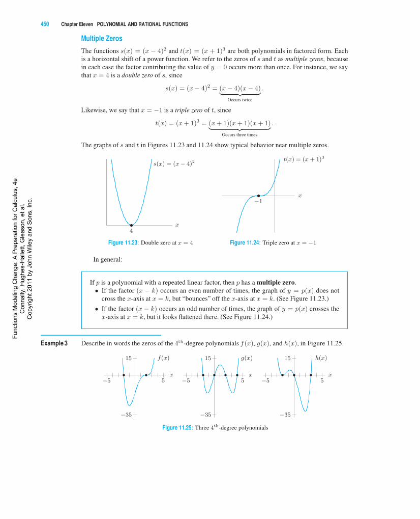
Multiple Zeros

The functions s(x) = (x − 4)2 and t(x) = (x + 1)3 are both polynomials in factored form. Eachis a horizontal shift of a power function. We refer to the zeros of s and t as multiple zeros, becausein each case the factor contributing the value of y = 0 occurs more than once. For instance, we saythat x = 4 is a double zero of s, since

s(x) = (x− 4)2 = (x− 4)(x− 4)︸︷︷︸Occurs twice

.

Likewise, we say that x = −1 is a triple zero of t, since

t(x) = (x + 1)3 = (x + 1)(x + 1)(x + 1)︸︷︷︸Occurs three times

.

The graphs of s and t in Figures 11.23 and 11.24 show typical behavior near multiple zeros.

4

s(x) = (x− 4)2

x

Figure 11.23: Double zero at x = 4

−1

t(x) = (x + 1)3

x

Figure 11.24: Triple zero at x = −1

In general:

If p is a polynomial with a repeated linear factor, then p has a multiple zero.• If the factor (x − k) occurs an even number of times, the graph of y = p(x) does not

cross the x-axis at x = k, but “bounces” off the x-axis at x = k. (See Figure 11.23.)

• If the factor (x − k) occurs an odd number of times, the graph of y = p(x) crosses thex-axis at x = k, but it looks flattened there. (See Figure 11.24.)

Example 3 Describe in words the zeros of the 4th-degree polynomials f(x), g(x), and h(x), in Figure 11.25.

−5 5

−35

15

x

f(x)

−5 5

−35

15

x

g(x)

−5 5

−35

15

x

h(x)

Figure 11.25: Three 4th-degree polynomials

Func

tions

Mod

elin

g C

hang

e: A

Pre

para

tion

for C

alcu

lus,

4e

Con

nally

, Hug

hes-

Hal

lett,

Gle

ason

, et a

l. C

opyr

ight

201

1 by

Joh

n W

iley

and

Son

s, In

c.


Solution The graph suggests that f has a single zero at x = −2. The flattened appearance near x = 2 suggeststhat f has a multiple zero there. Since the graph crosses the x-axis at x = 2 (instead of bouncingoff it), this zero must occur an odd number of times. Since f is 4th degree, f has at most 4 factors,so there must be a triple zero at x = 2.

The graph of g has four single zeros. The graph of h has two single zeros (at x = 0 and x = 3)and a double zero at x = −2. The multiplicity of the zero at x = −2 is not higher than two becauseh is of degree n = 4.

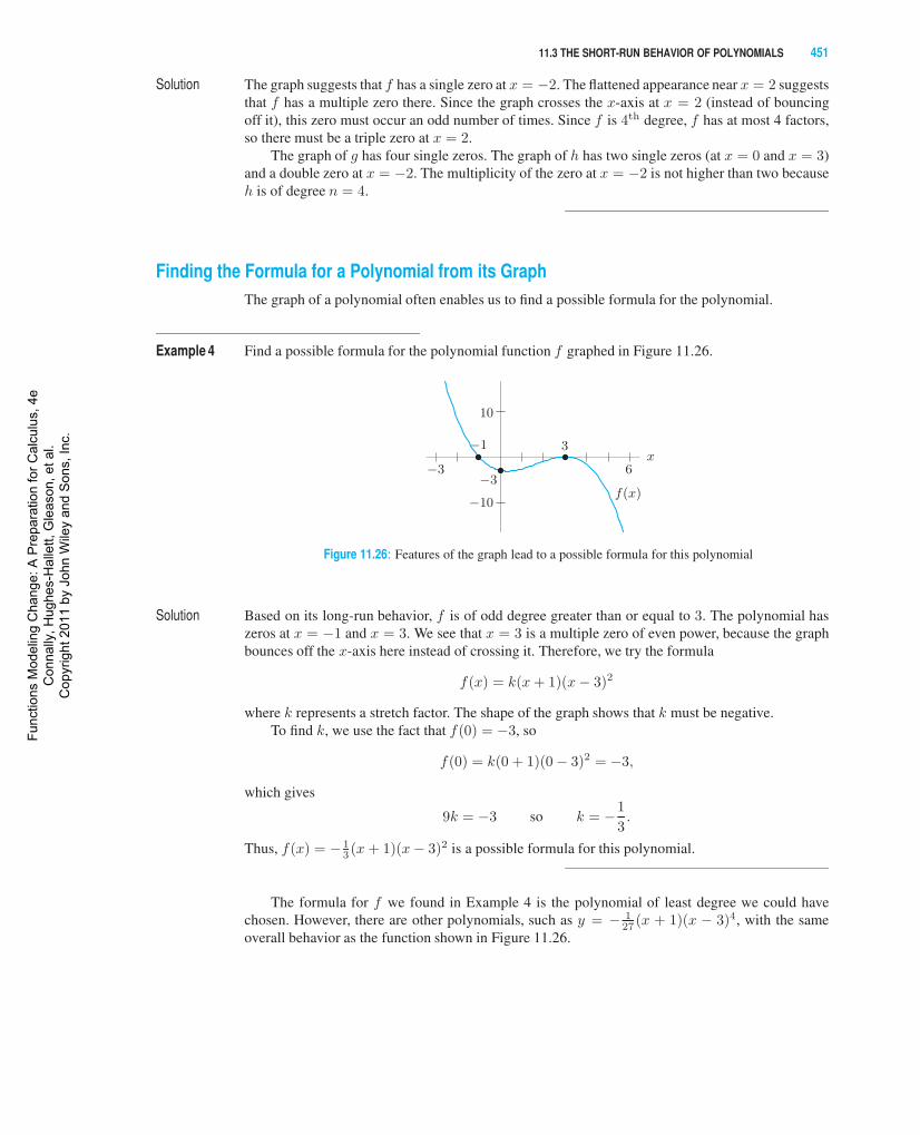
Finding the Formula for a Polynomial from its GraphThe graph of a polynomial often enables us to find a possible formula for the polynomial.

Example 4 Find a possible formula for the polynomial function f graphed in Figure 11.26.

−3

−1 3

6

−10

−3

10

f(x)

x

Figure 11.26: Features of the graph lead to a possible formula for this polynomial

Solution Based on its long-run behavior, f is of odd degree greater than or equal to 3. The polynomial haszeros at x = −1 and x = 3. We see that x = 3 is a multiple zero of even power, because the graphbounces off the x-axis here instead of crossing it. Therefore, we try the formula

f(x) = k(x + 1)(x− 3)2

where k represents a stretch factor. The shape of the graph shows that k must be negative.To find k, we use the fact that f(0) = −3, so

f(0) = k(0 + 1)(0− 3)2 = −3,

which gives

9k = −3 so k = −1

3.

Thus, f(x) = − 13 (x + 1)(x− 3)2 is a possible formula for this polynomial.

The formula for f we found in Example 4 is the polynomial of least degree we could havechosen. However, there are other polynomials, such as y = − 1

27 (x + 1)(x − 3)4, with the sameoverall behavior as the function shown in Figure 11.26.

Func

tions

Mod

elin

g C

hang

e: A

Pre

para

tion

for C

alcu

lus,

4e

Con

nally

, Hug

hes-

Hal

lett,

Gle

ason

, et a

l. C

opyr

ight

201

1 by

Joh

n W

iley

and

Son

s, In

c.



In Exercises 1–4, find the zeros of the functions.

1. y = x3 + 7x2 + 12x

2. y = (x2 + 2x− 7)(x3 + 4x2 − 21x)

3. y = 7(x + 3)(x− 2)(x + 7)

4. y = a(x + 2)(x− b), where a, b are nonzero constants

5. Use the graph of h(x) in Figure 11.21 on page 448 todetermine the factored form of

h(x) = x4 + x3 − 8x2 − 12x.

6. Use the graph of g(x) in Figure 11.21 on page 448 todetermine the factored form of

g(x) = x4 − 4x3 − 4x2 + 16x.

7. Use the graph of f(x) in Figure 11.21 on page 448 todetermine the factored form of

f(x) = x4 − 4x3 + 16x− 16.

8. Factor f(x) = 8x3 − 4x2 − 60x completely, and deter-mine the zeros of f .

9. Find a possible formula for a polynomial with zeros at(and only at) x = −2, 2, 5, a y-intercept at y = 5, andlong-run behavior of y → −∞ as x → ±∞.

Without a calculator, graph the polynomials in Exercises 10–11. Label all the x-intercepts and y-intercepts.

10. f(x) = −5(x2 − 4)(25− x2)

11. g(x) = 5(x− 4)(x2 − 25)

Problems

12. (a) Let f(x) = (2x− 1)(3x− 1)(x− 7)(x− 9). Whatare the zeros of this polynomial?

(b) Is it possible to find a viewing window that shows allof the zeros and all of the the turning points of f?

(c) Find two separate viewing windows that togethershow all the zeros and all the turning points of f.

13. (a) Experiment with various viewing windows to deter-mine the zeros of f(x) = 2x4+9x3−7x2−9x+5.Then write f in factored form.

(b) Find a single viewing window that clearly shows allof the turning points of f.

14. Let p(x) = x4 + 10x3 − 68x2 + 102x − 45. By exper-imenting with various viewing windows, determine thezeros of p and use this information to write p(x) in fac-tored form.

15. Without using a calculator, decide which of the equationsA–E best describes the polynomial in Figure 11.27.

A y = (x + 2)(x + 1)(x− 2)(x− 3)B y = x(x + 2)(x + 1)(x− 2)(x− 3)C y = − 1

2(x + 2)(x + 1)(x− 2)(x− 3)

D y = 12(x + 2)(x + 1)(x− 2)(x− 3)

E y = −(x + 2)(x + 1)(x− 2)(x− 3)

−3 1 4

−10

−5

5

Figure 11.27

In Problems 16–21, find a possible formula for each polyno-mial with the given properties.

16. f has degree ≤ 2, f(0) = 0 and f(1) = 1.

17. f has degree ≤ 2, f(0) = f(1) = f(2) = 1.

18. f has degree ≤ 2, f(0) = f(2) = 0 and f(3) = 3.

19. f is third degree with f(−3) = 0, f(1) = 0, f(4) = 0,and f(2) = 5.

20. g is fourth degree, g has a double zero at x = 3,g(5) = 0, g(−1) = 0, and g(0) = 3.

21. Least possible degree through the points (−3, 0), (1, 0),and (0,−3).

22. Which of these functions have inverses that are func-tions? Discuss.

(a) f(x) = (x− 2)3 + 4.(b) g(x) = x3 − 4x2 + 2.

Func

tions

Mod

elin

g C

hang

e: A

Pre

para

tion

for C

alcu

lus,

4e

Con

nally

, Hug

hes-

Hal

lett,

Gle

ason

, et a

l. C

opyr

ight

201

1 by

Joh

n W

iley

and

Son

s, In

c.


In Problems 23–32, give a possible formula for the polyno-mial.

23.

−1−2 21

−2

−1

1

2

x

yf(x) 24.

−2−1 1 2 3

−2

−1

1

x

y h(x)

25.

−1 1

2

−4

−2

2

4 f(x)

x

y

Note appearance near origin

26.−2

�(−1,−3)

2 3x

g(x)

y

27.

−1

1x

(− 12,− 27

16)

f(x)

y 28.

−4 3

4

f(x)

x

y

29.

−2

−1

1−2x

h(x)

y 30.

−2

(−1, 4)

(2, 4) (4, 4)

g(x)

y

x

31.

−1−2 21

−2

−1

1

2

x

y

g(x)

32.

−1 1−2 2

1

x

g(x)y

For Problems 33–38, find the real zeros (if any) of the poly-nomials.

33. y = 4x2 − 1 34. y = x4 + 6x2 + 9

35. y = (x2 − 8x + 12)(x− 3)

36. y = x2 + 5x + 6

37. y = 4x2 + 1

38. y = ax2(x2 + 4)(x + 3), where a is a nonzero constant.

39. Suppose the polynomial

f(x) = (x− 5)2(x− 3)2(x− 1)(x− r)(x + 3)s · g(x)

is an even function. What can you say about the constantsr, s and the second-degree polynomial function g(x)?

40. Find at least two different third-degree polynomials hav-ing zeros at x = −1 and x = 2 (and nowhere else), andy-intercept at y = 3.

41. An open-top box is to be constructed from a 6-in by 8-inrectangular sheet of tin by cutting out squares of equalsize at each corner, then folding up the resulting flaps.Let x denote the length of the side of each cut-out square.Assume negligible thickness.

(a) Find a formula for the volume of the box as a func-tion of x.

(b) For what values of x does the formula from part (a)make sense in the context of the problem?

(c) Sketch a graph of the volume function.(d) What, approximately, is the maximum volume of the

box?

42. You wish to pack a cardboard box inside a wooden crate.In order to have room for the packing materials, you needto leave a 0.5-ft space around the front, back, and sidesof the box, and a 1-ft space around the top and bottom ofthe box. If the cardboard box is x feet long, (x + 2) feetwide, and (x− 1) feet deep, find a formula in terms of xfor the amount of packing material needed.

43. Take an 8.5- by 11-inch piece of paper and cut out fourequal squares from the corners. Fold up the sides to cre-ate an open box. Find the dimensions of the box that hasmaximum volume.

44. Give the domain for g(x) = ln((x− 3)2(x + 2)

).

45. Given that a, b, and c are constants, a < b < c, state thedomain of

y =√

(x− a)(x− b)(x− c).

[Hint: Graph y = (x− a)(x− b)(x− c).]

Func

tions

Mod

elin

g C

hang

e: A

Pre

para

tion

for C

alcu

lus,

4e

Con

nally

, Hug

hes-

Hal

lett,

Gle

ason

, et a

l. C

opyr

ight

201

1 by

Joh

n W

iley

and

Son

s, In

c.


46. Consider the function a(x) = x5 + 2x3 − 4x.

(a) Without using a calculator or computer, what canyou say about the graph of a?

(b) Use a calculator or a computer to determine the ze-ros of this function to three decimal places.

(c) Explain why you think that you have all the possiblezeros.

(d) What are the zeros of b(x) = 2x5 +4x3−8x? Doesyour answer surprise you?

47. In each of the following cases, find a possible formula forthe polynomial f .

(a) Suppose f has zeros at x = −2, x = 3, x = 5 anda y-intercept of 4.

(b) In addition to the properties in part (a), suppose fhas the following long-run behavior: As x → ±∞,y → −∞. [Hint: Assume f has a double zero.]

(c) In addition to the properties in part (a), suppose f

has the following long-run behavior: As x → ±∞,y → +∞.

48. The following statements about f(x) are true:

• f(x) is a polynomial function• f(x) = 0 at exactly four different values of x• f(x)→ −∞ as x → ±∞

For each of the following statements, write true if thestatement must be true, never true if the statement isnever true, or sometimes true if it is sometimes true andsometimes not true.

(a) f(x) is an odd function(b) f(x) is an even function(c) f(x) is a fourth-degree polynomial(d) f(x) is a fifth-degree polynomial(e) f(−x)→ −∞ as x → ±∞(f) f(x) is invertible

11.4 RATIONAL FUNCTIONS

The Average Cost of Producing a Therapeutic DrugA pharmaceutical company wants to begin production of a new drug. The total cost C, in dollars,of making q grams of the drug is given by the linear function

C(q) = 2,500,000 + 2000q.

The fact that C(0) = 2,500,000 tells us that the company spends $2,500,000 before it starts makingthe drug. This quantity is known as the fixed cost because it does not depend on how much of thedrug is made. It represents the cost for research, testing, and equipment. In addition, the slope ofC tells us that each gram of the drug costs an extra $2000 to make. This quantity is known as thevariable cost per unit. It represents the additional cost, in labor and materials, to make an additionalgram of the drug.

The fixed cost of $2.5 million is large compared to the variable cost of $2000 per gram. Thismeans that it is impractical for the company to make a small amount of the drug. For instance, thetotal cost for 10 grams is

C(10) = 2,500,000 + 2000 · 10 = 2,520,000,

which works out to an average cost of $252,000 per gram. The company would probably never sellsuch an expensive drug.

However, as larger quantities of the drug are manufactured, the initial expenditure of $2.5 mil-lion seems less significant. The fixed cost averages out over a large quantity. For example, if thecompany makes 10,000 grams of the drug,

Average cost =Cost of producing 10,000 grams

10,000=

2,500,000 + 2000 · 10,000

10,000= 2250,

or $2250 per gram of drug produced.

Func

tions

Mod

elin

g C

hang

e: A

Pre

para

tion

for C

alcu

lus,

4e

Con

nally

, Hug

hes-

Hal

lett,

Gle

ason

, et a

l. C

opyr

ight

201

1 by

Joh

n W

iley

and

Son

s, In

c.

11.4 RATIONAL FUNCTIONS 455

10,000 20,000

2000

4000

6000

q, number of grams

y, average cost(dollars per gram)

a(q)

y = 2000: Horizontal asymptote

Figure 11.28: The graph of y = a(q), a rational function, has a horizontal asymptote at y = 2000 and avertical asymptote at q = 0

We define the average cost, a(q), as the cost per gram to produce q grams of the drug:

a(q) =Average cost of

producing q grams=

Total costNumber of grams

=C(q)

q=

2,500,000 + 2000q

q.

Figure 11.28 gives a graph of y = a(q) for q > 0. The horizontal asymptote reflects the fact that forlarge values of q, the value of a(q) is close to 2000. This is because, as more of the drug is produced,the average cost gets closer to $2000 per gram. See Table 11.9.

The vertical asymptote of y = a(q) is the y-axis, which tells us that the average cost per gram isvery large if a small amount of the drug is made. This is because the initial $2.5 million expenditureis averaged over very few units. We saw that producing only 10 grams costs a staggering $252,000per gram.

Table 11.9 As quantity q increases, the average cost a(q) draws closer to $2000 per gram

Quantity, q Total cost, C(q) = 2,500,000 + 2000q Average cost, a(q) = C(q)/q

10,000 2,500,000 + 20,000,000 = 22,500,000 2250

50,000 2,500,000 + 100,000,000 = 102,500,000 2050

100,000 2,500,000 + 200,000,000 = 202,500,000 2025

500,000 2,500,000 + 1,000,000,000 = 1,002,500,000 2005

What is a Rational Function?The formula for a(q) is the ratio of the polynomial 2,500,000 + 2000q and the polynomial q. Sincea(q) is given by the ratio of two polynomials, a(q) is an example of a rational function. In general:

If r can be written as the ratio of polynomial functions p(x) and q(x), that is, if

r(x) =p(x)

q(x),

then r is called a rational function. (We assume that q(x) is not the constant polynomialq(x) = 0.)

Func

tions

Mod

elin

g C

hang

e: A

Pre

para

tion

for C

alcu

lus,

4e

Con

nally

, Hug

hes-

Hal

lett,

Gle

ason

, et a

l. C

opyr

ight

201

1 by

Joh

n W

iley

and

Son

s, In

c.


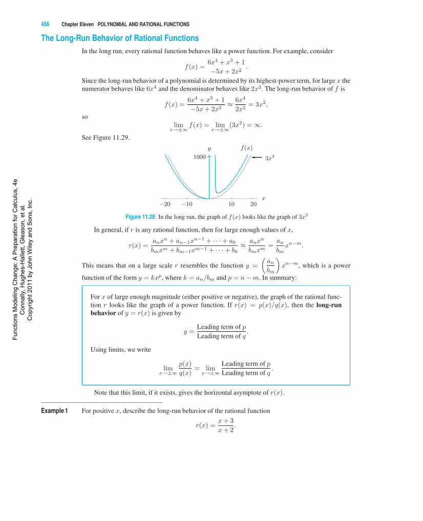
The Long-Run Behavior of Rational FunctionsIn the long run, every rational function behaves like a power function. For example, consider

f(x) =6x4 + x3 + 1

−5x + 2x2.

Since the long-run behavior of a polynomial is determined by its highest-power term, for large x thenumerator behaves like 6x4 and the denominator behaves like 2x2. The long-run behavior of f is

f(x) =6x4 + x3 + 1

−5x + 2x2≈ 6x4

2x2= 3x2,

solim

x→±∞f(x) = lim

x→±∞(3x2) = ∞.

See Figure 11.29.

−20 −10 10 20

1000

f(x)

� 3x2

x

y

Figure 11.29: In the long run, the graph of f(x) looks like the graph of 3x2

In general, if r is any rational function, then for large enough values of x,

r(x) =anxn + an−1x

n−1 + · · ·+ a0

bmxm + bm−1xm−1 + · · ·+ b0≈ anxn

bmxm=

an

bmxn−m.

This means that on a large scale r resembles the function y =

(an

bm

)xn−m, which is a power

function of the form y = kxp, where k = an/bm and p = n−m. In summary:

For x of large enough magnitude (either positive or negative), the graph of the rational func-tion r looks like the graph of a power function. If r(x) = p(x)/q(x), then the long-runbehavior of y = r(x) is given by

y =Leading term of p

Leading term of q.

Using limits, we write

limx→±∞

p(x)

q(x)= lim

x→±∞

Leading term of p

Leading term of q.

Note that this limit, if it exists, gives the horizontal asymptote of r(x).

Example 1 For positive x, describe the long-run behavior of the rational function

r(x) =x + 3

x + 2.

Func

tions

Mod

elin

g C

hang

e: A

Pre

para

tion

for C

alcu

lus,

4e

Con

nally

, Hug

hes-

Hal

lett,

Gle

ason

, et a

l. C

opyr

ight

201

1 by

Joh

n W

iley

and

Son

s, In

c.


Solution If x is a large positive number, then

r(x) =Big number + 3

Same big number + 2≈ Big number

Same big number= 1.

For example, if x = 100, we have

r(x) =103

102= 1.0098 . . . ≈ 1.

If x = 10,000, we have

r(x) =10, 003

10, 002= 1.00009998 . . .≈ 1,

For large positive x-values, r(x) ≈ 1. Thus, for large enough values of x, the graph of y = r(x)looks like the line y = 1, its horizontal asymptote. We write limx→∞ r(x) = 1. See Figure 11.30.However, for x > 0, the graph of r is above the line since the numerator is larger than the denomi-nator.

5 10 15 20 25

1

1.5

x

y

y =x + 3

x + 2y = 1: Horizontal

asymptote

Figure 11.30: For large positive values of x, the graph ofr(x) = (x + 3)/(x + 2) looks like the horizontal line y = 1

Example 2 For positive x, describe the positive long-run behavior of the rational function

g(x) =3x + 1

x2 + x− 2.

Solution The leading term in the numerator is 3x and the leading term in the denominator is x2. Thus forlarge enough values of x,

g(x) ≈ 3x

x2=

3

x,

so

limx→∞

g(x) = limx→∞

(3

x

)= 0.

Figure 11.31 shows the graphs of y = g(x) and y = 3/x. For large values of x, the two graphs arenearly indistinguishable. Both graphs have a horizontal asymptote at y = 0.

5x

y

y = g(x)

� y = 3/x: Shows long-run behavioras x →∞

Figure 11.31: For large enough values of x, the function g looks like the function y = 3x−1

Func

tions

Mod

elin

g C

hang

e: A

Pre

para

tion

for C

alcu

lus,

4e

Con

nally

, Hug

hes-

Hal

lett,

Gle

ason

, et a

l. C

opyr

ight

201

1 by

Joh

n W

iley

and

Son

s, In

c.


What Causes Asymptotes?The graphs of rational functions often behave differently from the graphs of polynomials. Polyno-mial graphs (except constant functions) cannot level off to a horizontal line as the graphs of rationalfunctions can. In Example 1, the numerator and denominator are approximately equal for large x,producing the horizontal asymptote y = 1. In Example 2, the denominator grows faster than thenumerator, driving the quotient toward zero.

The rapid rise (or fall) of the graph of a rational function near its vertical asymptote is due tothe denominator becoming small (close to zero). It is tempting to assume that any function that hasa denominator has a vertical asymptote. However, this is not true. To have a vertical asymptote, thedenominator must equal zero. For example, suppose that

r(x) =1

x2 + 3.

The denominator is always greater than 3; it is never 0. We see from Figure 11.32 that r does nothave a vertical asymptote.

−3 3

y = r(x)

12

x

y

Figure 11.32: The rational function r(x) = 1/(x2 + 3) has no vertical asymptote

Exercises and Problems for Section 11.4Skill Refresher

For Exercises S1–S4, perform the operations. Express an-swers in reduced form.

S1.6

y+

7

y3S2.

13

x− 1+

14

2x− 2

S3.

1

x− 2

x2

2x− 4

x5

S4.9

x2 + 5x + 6+

12

x + 3

S5.5

(x− 2)2(x + 1)− 18

(x− 2)

In Exercises S6–S9, simplify, if possible.

S6.1/(x + y)

x + yS7.

(w + 2)/2

w + 2

S8.a2 − b2

a2 + b2S9.

x−1 + x−2

1− x−2.

Exercises

Are the functions in Exercises 1–7 rational functions? If so,write them in the form p(x)/q(x), the ratio of polynomials.

1. f(x) =x + 2

x2 − 12. f(x) =

4x + 3

3x − 1

3. f(x) =x2

2+

1

x4. f(x) =

x4 + 3x − x2

x3 − 2

5. f(x) =

√x + 1

x + 16. f(x) =

x3

2x2+

1

6

7. f(x) =9x− 1

4√

x + 7+

5x3

x2 − 1

Evaluate the limits in Exercises 8–11.

8. limx→∞

(2x−3 + 4) 9. limx→∞

(3x−2 + 5x + 7)

10. limx→∞

4x + 3x2

4x2 + 3x11. lim

x→−∞

3x2 + x

2x2 + 5x3

Func

tions

Mod

elin

g C

hang

e: A

Pre

para

tion

for C

alcu

lus,

4e

Con

nally

, Hug

hes-

Hal

lett,

Gle

ason

, et a

l. C

opyr

ight

201

1 by

Joh

n W

iley

and

Son

s, In

c.


Find the horizontal asymptote, if it exists, of the functions inExercises 12–14.

12. h(x) = 3− 1

x+

x

x + 1

13. f(x) =1

1 +1

x

14. g(x) =(1− x)(2 + 3x)

2x2 + 1

15. Compare and discuss the long-run behaviors of the fol-lowing functions:

f(x) =x2 + 1

x2 + 5, g(x) =

x3 + 1

x2 + 5, h(x) =

x + 1

x2 + 5.

Problems

16. Find a formula for f−1(x) given that

f(x) =4− 3x

5x− 4.

17. Give examples of rational functions with even symmetry,odd symmetry, and neither. How does the symmetry off(x) = p(x)/q(x) depend on the symmetry of p(x) andq(x)?

18. Let r(x) = p(x)/q(x), where p and q are polynomialsof degrees m and n, respectively. What conditions on mand n ensure that the following statements are true?

(a) limx→∞

r(x) = 0

(b) limx→∞

r(x) = k, with k �= 0.

19. Let t be the time in weeks. At time t = 0, organic wasteis dumped into a pond. The oxygen level in the pond attime t is given by

f(t) =t2 − t + 1

t2 + 1.

Assume f(0) = 1 is the normal level of oxygen.

(a) Graph this function.(b) Describe the shape of the graph. What is the signifi-

cance of the minimum for the pond?(c) What eventually happens to the oxygen level?(d) Approximately how many weeks must pass before

the oxygen level returns to 75% of its normal level?

20. A small printing house agrees to publish a book of po-ems illustrated by the author. The printing house plans torecover its investment of $80,000 and make a profit of$40,000. The price of the book will depend on the num-ber of copies they expect to sell.

(a) Fill in the table with the price per copy for each pro-jected sales figure.

Number of copies sold 1000 2000 4000 6000

Price per copy

(b) Give a formula for the price per copy, p, as a functionof projected sales, s.

(c) Graph the function p = f(s).

21. Bronze is an alloy, or mixture, of copper and tin. The al-loy initially contains 3 kg copper and 9 kg tin. You add xkg of copper to this 12 kg of alloy. The concentration ofcopper in the alloy is a function of x:

f(x) = Concentration of copper =Total amount of copperTotal amount of alloy

.

(a) Find a formula for f in terms of x, the amount ofcopper added.

(b) Evaluate the following expressions and explain theirsignificance for the alloy:

(i) f( 12) (ii) f(0) (iii) f(−1)

(iv) f−1( 12) (v) f−1(0)

(c) Graph f(x) for −5 ≤ x ≤ 5, −0.25 ≤ y ≤ 0.5.Interpret the intercepts in the context of the alloy.

(d) Graph f(x) for −3 ≤ x ≤ 100, 0 ≤ y ≤ 1.Describe the appearance of your graph for large x-values. Does the appearance agree with what you ex-pect to happen when large amounts of copper areadded to the alloy?

22. A chemist is studying the properties of a bronze alloy(mixture) of copper and tin. She begins with 2 kg of analloy that is one-half tin. Keeping the amount of copperconstant, she adds small amounts of tin to the alloy. Let-ting x be the total amount of tin added, define

C(x) = Concentration of tin =Total amount of tin

Total amount of alloy.

(a) Find a formula for C(x).(b) Evaluate C(0.5) and C(−0.5). Explain the physical

significance of these quantities.(c) Graph y = C(x), labeling all interesting features.

Describe the physical significance of the featuresyou have labeled.

Func

tions

Mod

elin

g C

hang

e: A

Pre

para

tion

for C

alcu

lus,

4e

Con

nally

, Hug

hes-

Hal

lett,

Gle

ason

, et a

l. C

opyr

ight

201

1 by

Joh

n W

iley

and

Son

s, In

c.


23. The population of Mathville has been increasing since2010 when it was 12,000. If the population t years after2010 is

P (t) = 20(

4t + 3

2t + 5

)thousand,

when will the population of Mathville reach 20,000?When will it reach 50,000?

24. A car is driven for 60 miles. The first 10 miles arethrough a large city at a speed of 40 mph; once out ofthe city a speed of V mph is maintained.

(a) Calculate the average speed for the 60-mile trip.(b) If you want to average 60 mph for the trip, how fast

need you go during the last 50 miles?

25. An alcohol solution consists of 5 gallons of pure waterand x gallons of alcohol, x > 0. Let f(x) be the ratioof the volume of alcohol to the total volume of liquid.[Note that f(x) is the concentration of the alcohol in thesolution.]

(a) Find a possible formula for f(x).(b) Evaluate and interpret f(7) in the context of the mix-

ture.(c) What is the zero of f? Interpret your result in the

context of the mixture.(d) Find an equation for the horizontal asymptote of f .

Explain its significance in the context of the mixture.

26. The total cost C(n) for a producer to manufacture n unitsof a good is given by

C(n) = 5000 + 50n.

The average cost of producing n units is a(n) =C(n)/n.

(a) Evaluate and interpret the economic significance of:

(i) C(1) (ii) C(100)(iii) C(1000) (iv) C(10000)

(b) Evaluate and interpret the economic significance of:

(i) a(1) (ii) a(100)(iii) a(1000) (iv) a(10000)

(c) Based on part (b), what trend do you notice in thevalues of a(n) as n gets large? Explain this trend ineconomic terms.

27. Figure 11.33 shows the cost function, C(n), from Prob-lem 26, and a line, l, that passes through the origin.

(a) What is the slope of line l?(b) How does line l relate to a(n0), the average cost of

producing n0 units (as defined in Problem 26)?

n0

5000

C(n)l

n

Figure 11.33

28. Typically, the average cost of production (as defined inProblem 26) decreases as the level of production in-creases. Is this always the case for the goods whose totalcost function is graphed in Figure 11.34? Use the resultof Problem 27 and explain your reasoning.

n1 n2

l1

l2

Total cost

Figure 11.34

29. It costs a company $30,000 to begin production of agood, plus $3 for every unit of the good produced. Letx be the number of units produced by the company.

(a) Find a formula for C(x), the total cost for the pro-duction of x units of the good.

(b) Find a formula for the company’s average cost perunit, a(x).

(c) Graph y = a(x) for 0 < x ≤ 50,000, 0 ≤ y ≤ 10.Label the horizontal asymptote.

(d) Explain in economic terms why the graph of a hasthe long-run behavior that it does.

(e) Explain in economic terms why the graph of a hasthe vertical asymptote that it does.

(f) Find a formula for a−1(y). Give an economic inter-pretation of a−1(y).

(g) The company makes a profit if the average cost ofits good is less than $5 per unit. Find the minimumnumber of units the company can produce and makea profit.

Func

tions

Mod

elin

g C

hang

e: A

Pre

para

tion

for C

alcu

lus,

4e

Con

nally

, Hug

hes-

Hal

lett,

Gle

ason

, et a

l. C

opyr

ight

201

1 by

Joh

n W

iley

and

Son

s, In

c.

11.5 THE SHORT-RUN BEHAVIOR OF RATIONAL FUNCTIONS 461

30. Find a rational function of the form

R(x) =1

1 + cx

whose values equal those of f(x) = ex at x = 0 andx = 1. Plot and compare your approximation on the in-terval (0, 1) and comment on the result.

11.5 THE SHORT-RUN BEHAVIOR OF RATIONAL FUNCTIONS

The short-run behavior of a polynomial can often be determined from its factored form. The sameis true of rational functions. If r is a rational function given by

r(x) =p(x)

q(x), p, q polynomials,

then the short-run behaviors of p and q tell us about the short-run behavior of r.

The Zeros and Vertical Asymptotes of a Rational FunctionA fraction is equal to zero if and only if its numerator equals zero (and its denominator does notequal zero). Thus, the rational function r(x) = p(x)/q(x) has a zero wherever p has a zero, providedq does not have a zero there.

Just as we can find the zeros of a rational function by looking at its numerator, we can findthe vertical asymptotes by looking at its denominator. A rational function is large wherever itsdenominator is small. This means that r has a vertical asymptote wherever its denominator has azero, provided its numerator does not also have a zero there.

Example 1 Find the zeros and vertical asymptotes of the rational function r(x) =x + 3

x + 2.

Solution We see that r(x) = 0 ifx + 3

x + 2= 0.

This ratio equals zero only if the numerator is zero (and the denominator is not zero), so

x + 3 = 0

x = −3.

The only zero of r is x = −3. To check, note that r(−3) = 0/(−1) = 0. The denominator has azero at x = −2, so the graph of r(x) has a vertical asymptote there. Note that as x approaches −2from the left r(x) tends toward −∞ and as x approaches−2 from the right r(x) tends toward∞.

Example 2 Graph r(x) =25

(x + 2)(x− 3)2, showing all the important features.

Solution Since the numerator of this function is never zero, r has no zeros, meaning that the graph of r nevercrosses the x-axis. The graph of r has vertical asymptotes at x = −2 and x = 3 because this iswhere the denominator is zero. What does the graph of r look like near its asymptote at x = −2?

Func

tions

Mod

elin

g C

hang

e: A

Pre

para

tion

for C

alcu

lus,

4e

Con

nally

, Hug

hes-

Hal

lett,

Gle

ason

, et a

l. C

opyr

ight

201

1 by

Joh

n W

iley

and

Son

s, In

c.


At x = −2, the numerator is 25 and the value of the factor (x − 3)2 is (−2− 3)2 = 25. Thus, nearx = −2,

r(x) =25

(x + 2)(x− 3)2≈ 25

(x + 2)(25)=

1

x + 2.

So, near x = −2, the graph of r looks like the graph of y = 1/(x + 2). Note that the graph ofy = 1/(x + 2) is the graph of y = 1/x shifted to the left by 2 units. We see that

limx→−2−

r(x) = −∞ and limx→−2+

r(x) =∞.

−4 −3

−1 1 2

−4

6

x

yy = r(x)

y = 1x+2

y = 1x+2

� y = r(x)

x = −2

�Verticalasymptote

Figure 11.35: The rational function r resembles theshifted power function 1/(x + 2) near the

asymptote at x = −2

4 5−1 1 2

−4

6

x

y

� Verticalasymptote

y = r(x)

x = 3

y = 5

(x−3)2

Figure 11.36: The rational function rresembles the shifted power function

5/(x− 3)2 near the asymptote at x = 3

What does the graph of r look like near its vertical asymptote at x = 3? Near x = 3, thenumerator is 25 and value of the factor (x + 2) is approximately (3 + 2) = 5. Thus, near x = 3,

r(x) ≈ 25

(5)(x− 3)2=

5

(x− 3)2.

Near x = 3, the graph of r looks like the the graph of y = 5/(x− 3)2. We see that

limx→3

r(x) =∞.

The graph of y = 5/(x− 3)2 is the graph of y = 5/x2 shifted to the right 3 units. Since

r(0) =25

(0 + 2)(0− 3)2=

25

18≈ 1.4,

the graph of r crosses the y-axis at 25/18. The long-run behavior of r is given by the ratio of theleading term in the numerator to the leading term in the denominator. The numerator is 25, and ifwe multiply out the denominator, we see that its leading term is x3. Thus, the long-run behavior ofr is given by y = 25/x3, which has a horizontal asymptote at y = 0. See Figure 11.37. We see that

limx→±∞

r(x) = 0.

Func

tions

Mod

elin

g C

hang

e: A

Pre

para

tion

for C

alcu

lus,

4e

Con

nally

, Hug

hes-

Hal

lett,

Gle

ason

, et a

l. C

opyr

ight

201

1 by

Joh

n W

iley

and

Son

s, In

c.


−5 5

−5

5

x

y

�

y-intercept =25

18

� Verticalasymptotes

�

x = −2 x = 3

y = r(x)

�

Horizontalasymptoteat y = 0

Figure 11.37: A graph of the rational function r(x) =25

(x + 2)(x− 3)2, showing intercepts and asymptotes

The Graph of a Rational FunctionWe can now summarize what we have learned about the graphs of rational functions.

If r is a rational function given by r(x) =p(x)

q(x), where p and q are polynomials with different

zeros, then:• The long-run behavior and horizontal asymptote (if any) of r are given by the ratio of

the leading terms of p and q.

• The zeros of r are the same as the zeros of the numerator, p.

• The graph of r has a vertical asymptote at each of the zeros of the denominator, q.

If p and q have zeros at the same x-values, the rational function may behave differently. See thediscussion about holes in graphs on page 465.

Can a Graph Cross an Asymptote?

The graph of a rational function never crosses a vertical asymptote. However, the graphs of some ra-tional functions cross their horizontal asymptotes. The difference is that a vertical asymptote occurswhere the function is undefined, so there can be no y-value there, whereas a horizontal asymptoterepresents the limiting value of the function as x→ ±∞. There is no reason that the function cannot

take on this limiting y-value for some finite x-value. For example, the graph of r(x) =x2 + 2x− 3

x2

crosses the line y = 1, its horizontal asymptote; the graph does not cross the vertical asymptote, they-axis. See Figure 11.38.

2

2

y = 1

r(x)

x

y

Figure 11.38: A rational function can cross its horizontal asymptote

Func

tions

Mod

elin

g C

hang

e: A

Pre

para

tion

for C

alcu

lus,

4e

Con

nally

, Hug

hes-

Hal

lett,

Gle

ason

, et a

l. C

opyr

ight

201

1 by

Joh

n W

iley

and

Son

s, In

c.


Rational Functions as Transformations of Power FunctionsThe average cost function on page 455 can be written as

a(q) =2,500,000 + 2000q

q= 2,500,000q−1 + 2000.

Thus, the graph of a is the graph of the power function y = 2,500,000q−1 shifted up 2000 units.Many rational functions can be viewed as translations of power functions.

Finding a Formula for a Rational Function from its GraphThe graph of a rational function can give a good idea of its formula. Zeros of the function correspondto factors in the numerator and vertical asymptotes correspond to factors in the denominator.

Example 3 Find a possible formula for the rational function, g(x), graphed in Figure 11.39.

5−10 −5 �(−1, 0)

−1

1

0.5

x

y

y = g(x)

x = −2

Figure 11.39: The graph of y = g(x), a rational function

Solution From the graph, we see that g has a zero at x = −1 and a vertical asymptote at x = −2. Thismeans that the numerator of g has a zero at x = −1 and the denominator of g has a zero at x = −2.The zero of g does not seem to be a multiple zero because the graph crosses the x-axis instead ofbouncing and does not have a flattened appearance. Thus, we conclude that the numerator of g hasone factor of (x + 1).

The values of g(x) have the same sign on both sides of the vertical asymptote. Thus, the be-havior of g near its vertical asymptote is more like the behavior of y = 1/(x + 2)2 than likey = 1/(x + 2). We conclude that the denominator of g has a factor of (x + 2)2. This suggests

g(x) = k · x + 1

(x + 2)2,

where k is a stretch factor. To find the value of k, use the fact that g(0) = 0.5. So

0.5 = k · 0 + 1

(0 + 2)2

0.5 = k · 1

4k = 2.

Thus, a possible formula for g is g(x) =2(x + 1)

(x + 2)2.

Func

tions

Mod

elin

g C

hang

e: A

Pre

para

tion

for C

alcu

lus,

4e

Con

nally

, Hug

hes-

Hal

lett,

Gle

ason

, et a

l. C

opyr

ight

201

1 by

Joh

n W

iley

and

Son

s, In

c.


When Numerator and Denominator Have the Same Zeros: Holes

The rational function h(x) =x2 + x− 2

x− 1is undefined at x = 1 because the denominator equals

zero at x = 1. However, the graph of h does not have a vertical asymptote at x = 1 because thenumerator of h also equals zero at x = 1. At x = 1,

h(1) =x2 + x− 2

x− 1=

12 + 1− 2

1− 1=

0

0,

and this ratio is undefined. What does the graph of h look like? Factoring the numerator of h gives

h(x) =(x− 1)(x + 2)

x− 1=

x− 1

x− 1(x + 2).

For any x �= 1, we can cancel (x− 1) top and bottom and rewrite the formula for h as

h(x) = x + 2, provided x �= 1.

Thus, the graph of h is the line y = x+2 except at x = 1, where h is undefined. The line y = x+2contains the point (1, 3), but the graph of h does not. Therefore, we say that the graph of h has ahole in it at the point (1, 3). See Figure 11.40.

−3 −2 −1 1 2 3−1

1

2

3

4

5

x

yy = h(x)

(1, 3)� Hole

Figure 11.40: The graph of y = h(x) is the line y = x + 2, except at the point (1, 3), where it has a hole


For the rational functions in Exercises 1–4, find all zeros andvertical asymptotes and describe the long-run behavior, thengraph the function.

1. y =x− 4

x2 − 92. y =

x2 − 4

x− 9

3. y =x + 3

x + 54. y =

x + 3

(x + 5)2

In Exercises 5–8, what are the x-intercepts, y-intercepts, and

horizontal and vertical asymptotes (if any)?

5. h(x) =x2 − 4

x3 + 4x26. k(x) =

x(4− x)

x2 − 6x + 5

7. f(x) =x− 2

x− 48. g(x) =

x2 − 9

x2 + 9

Func

tions

Mod

elin

g C

hang

e: A

Pre

para

tion

for C

alcu

lus,

4e

Con

nally

, Hug

hes-

Hal

lett,

Gle

ason

, et a

l. C

opyr

ight

201

1 by

Joh

n W

iley

and

Son

s, In

c.


9. Let G(x) =2x

x + 4.

(a) Complete Table 11.10 for x-values close to −4.What happens to the values of G(x) as x approaches−4 from the left? From the right?

Table 11.10

x −5 −4.1 −4.01 −4 −3.99 −3.9 −3

G(x)

(b) Complete Tables 11.11 and 11.12. What happensto the values of G(x) as x takes very large positivevalues? As x takes very large negative values?

Table 11.11

x 5 10 100 1000

G(x)

Table 11.12

x −5 −10 −100 −1000

G(x)

(c) Without a calculator, graph y = G(x). Give equa-tions for the horizontal and vertical asymptotes.

10. Let g(x) =1

(x + 2)2.

(a) Complete Table 11.13 for x-values close to −2.What happens to the values of g(x) as x approaches−2 from the left? From the right?

Table 11.13

x −3 −2.1 −2.01 −2 −1.99 −1.9 −1

g(x)

(b) Complete Tables 11.14 and 11.15. What happens tothe values of g(x) as x takes very large positive val-ues? As x takes very large negative values?

Table 11.14

x 5 10 100 1000

g(x)

Table 11.15

x −5 −10 −100 −1000

g(x)

(c) Without a calculator, graph y = g(x). Give equa-tions for the horizontal and vertical asymptotes.

Problems

Graph the functions in Problems 11–12 without a calculator.

11. y = 2 +1

x12. y =

2x2 − 10x + 12

x2 − 16

In Problems 13–14, estimate the one-sided limits:

(a) limx→a+

f(x) (b) limx→a−

f(x)

13. f(x) =x

5− xwith a = 5

14. f(x) =5− x

(x− 2)2with a = 2

15. Without a calculator, match the functions (a)–(f) withtheir graphs in (i)–(vi) by finding the zeros, asymptotes,and end behavior for each function.

(a) y =−1

(x− 5)2− 1 (b) y =

x− 2

(x + 1)(x− 3)

(c) y =2x + 4

x− 1(d) y =

1

x + 1+

1

x− 3

(e) y =1− x2

x− 2(f) y =

1− 4x

2x + 2

−1

2 3x

y(i)

−2 1

2

x

y

y = 2

x = 1

(ii)

−1

x = 5

y = −1x

y(iii)

x = −1

x = 3

1x

y(iv)

x = −1

y = −2

x

y(v)

x = 2

x

y(vi)

Func

tions

Mod

elin

g C

hang

e: A

Pre

para

tion

for C

alcu

lus,

4e

Con

nally

, Hug

hes-

Hal

lett,

Gle

ason

, et a

l. C

opyr

ight

201

1 by

Joh

n W

iley

and

Son

s, In

c.


16. Let f(x) = x2 − 4, g(x) = x2 + 4, and h(x) = x + 5.Without a calculator, match the functions in (a)–(f) tothe descriptions in (i)–(viii). Some of the functions maymatch none of the descriptions.

(a) y =f(x)

g(x)(b) y =

g(x)

f(x)(c) y =

h(x)

f(x)

(d) y = f(1

x) (e) y =

g(x)

h(x)(f) y =

h(x2)

h(x)

(g) y =1

g(x)(h) y = f(x)·g(x)

(i) Horizontal asymptote at y = 0 and one zero atx = −5.

(ii) No horizontal asymptote, no zeros, and a verticalasymptote at x = −5.

(iii) Zeros at x = −5, x = −2, and x = 2.(iv) No zeros, a horizontal asymptote at y = 0, and a

vertical asymptote at x = −5.(v) Two zeros, no vertical asymptotes, and a horizontal

asymptote at y = 1.(vi) No zeros, no vertical asymptotes, and a horizontal

asymptote at y = 1.(vii) Horizontal asymptote at y = −4.

(viii) No horizontal asymptotes, two zeros, and a verticalasymptote at x = −5.

In Problems 17–18,

(a) Estimate limx→∞

f(x) and limx→−∞

f(x).

(b) What does the vertical asymptote tell you about limits?

17.

−7 −2 3−2

8

x

y 18.

−14 −4 6

−10

2

10

x

y

19. Suppose that n is a constant and that f(x) is a functiondefined when x = n. Complete the following sentences.

(a) If f(n) is large, then1

f(n)is . . .

(b) If f(n) is small, then1

f(n)is . . .

(c) If f(n) = 0, then1

f(n)is . . .

(d) If f(n) is positive, then1

f(n)is . . .

(e) If f(n) is negative, then1

f(n)is . . .

20. (a) Use the results of Problem 19 to graph y = 1/f(x)given the graph of y = f(x) in Figure 11.41.

(b) Find a possible formula for the function in Fig-ure 11.41. Use this formula to check your graph forpart (a).

1 2

1x

y

f(x)

Figure 11.41

21. Use the graph of f in Figure 11.42 to graph

(a) y = −f(−x) + 2 (b) y =1

f(x)

−1 3−2

2 f(x)

Figure 11.42

Problems 22–24 show a transformation of y = 1/x.

(a) Find a possible formula for the graph.

(b) Write the formula from part (a) as the ratio of two linearpolynomials.

(c) Find the coordinates of the intercepts of the graph.

22.

−2−4−6 2 4 6

−6

−4

−2

2

4

6

x

y 23.

−2−4−6

2 4 6

−6

−4

−2

2

4

6

x

y

24.

−2−4−6 2 4 62

−6

−4

−2

2

4

6

x

y

Func

tions

Mod

elin

g C

hang

e: A

Pre

para

tion

for C

alcu

lus,

4e

Con

nally

, Hug

hes-

Hal

lett,

Gle

ason

, et a

l. C

opyr

ight

201

1 by

Joh

n W

iley

and

Son

s, In

c.


Each of the functions in Problems 25–27 is a transformationof y = 1/xp. For each function, determine p, describe thetransformation in words, and graph the function, labeling anyintercepts and asymptotes.

25. f(x) =1

x− 3+ 4

26. g(x) = − 1

(x− 2)2− 3

27. h(x) =1

x− 1+

2

1− x+ 2

Problems 28–31 give values of transformations of either y =1/x or y = 1/x2. In each case

(a) Determine if the values are from a transformation ofy = 1/x or y = 1/x2. Explain your reasoning.

(b) Find a possible formula for the function.

28.x y

−1000 1.000001

−100 1.00001

−10 1.01

10 1.01

100 1.0001

1000 1.000001

29.x y

1.5 −1.5

1.9 −9.5

1.95 −19.5

2 Undefined

2.05 20.5

2.1 10.5

2.5 2.5

30.x y

2.7 12.1

2.9 101

2.95 401

3 Undefined

3.05 401

3.1 101

3.3 12.1

31.x y

−1000 0.499

−100 0.490

−10 0.400

10 0.600

100 0.510

1000 0.501

32. Cut four equal squares from the corners of a 8.5′′ × 11′′

piece of paper. Fold up the sides to create an open box.Find the dimensions of the box with the maximum vol-ume per surface area.

Find possible formulas for the functions in Problems 33–38.33.

−1x

y

x = 2

y = −1

�

(0, 0.5)

34.

−3

x = −2

1−34

y = 1

x

y

35.

x = −1

−2

x = 2

3

−3

x

y = −1

y 36.

−2

x = −1

y

(0, 3)

x = 2

3x

y = 1

37.

2

2

x = −1 x = 1

x

y 38.x = −2

x = 3

x

y

39. The graph of f(x) =18− 11x + x2

x− 2is a line with a

hole in it. What is the equation of the line? What are thecoordinates of the hole?

40. The graph of g(x) =x3 + 5x2 + x + 5

x + 5is a parabola

with a hole in it. What is the equation of the parabola?What are the coordinates of the hole?

41. Write a formula for a function, h(x), whose graph isidentical to the graph of y = x3, except that the graphof h has a hole at (2, 8). Express the formula as a ratio oftwo polynomials

In Problems 42–44, find a possible formula for the rationalfunctions.

42. This function has zeros at x = 2 and x = 3. It has a ver-tical asymptote at x = 5. It has a horizontal asymptoteof y = −3.

43. The graph of y = g(x) has two vertical asymptotes: oneat x = −2 and one at x = 3. It has a horizontal asymp-tote of y = 0. The graph of g crosses the x-axis once, atx = 5.

44. The graph of y = h(x) has two vertical asymptotes: oneat x = −2 and one at x = 3. It has a horizontal asymp-tote of y = 1. The graph of h touches the x-axis once, atx = 5.

Func

tions

Mod

elin

g C

hang

e: A

Pre

para

tion

for C

alcu

lus,

4e

Con

nally

, Hug

hes-

Hal

lett,

Gle

ason

, et a

l. C

opyr

ight

201

1 by

Joh

n W

iley

and

Son

s, In

c.

11.6 COMPARING POWER, EXPONENTIAL, AND LOG FUNCTIONS 469

11.6 COMPARING POWER, EXPONENTIAL, AND LOG FUNCTIONS

In preceding chapters, we encountered exponential and logarithmic functions. In this section, wecompare the long- and short-run behaviors of these functions and power functions.

Comparing Power FunctionsFor power functions y = kxp for large x, the higher the power of x, the faster the function climbs.See Figure 11.43. Not only are the higher powers larger, but they are much larger. This is because ifx = 100, for example, 1005 is one hundred times as big as 1004, which is one hundred times as bigas 1003. As x gets larger (written as x → ∞), any positive power of x grows much faster than alllower powers of x. We say that, as x→∞, higher powers of x dominate lower powers.

As x approaches zero (written x→ 0), the situation is reversed. Figure 11.44 is a close-up viewnear the origin. For x between 0 and 1, x3 is bigger than x4, which is bigger than x5. (Try x = 0.1to confirm this.) For values of x near zero, smaller powers dominate.

1 2 3 4

5

10

15

x

y

x

x1.5

x2

x3x4x5

Figure 11.43: For large x: Large powers of xdominate

1

1

x

y

x

x1.5

x2

x3

x4

x5

�

�

�

�

�

�

Figure 11.44: For 0 ≤ x ≤ 1: Small powers of xdominate

In Chapter 6 we saw the effect of k on the graph of f(x) = kxp. The coefficient k stretches orcompresses the graph vertically; if k is negative, the graph is reflected across the x-axis. How doesthe value of k affect the long-term growth rate of f(x) = kxp? Is the growth of a power functionaffected more by the size of the coefficient or by the size of the power?

Example 1 Let f(x) = 100x3 and g(x) = x4 for x > 0. Compare the long-term behavior of these two functionsusing graphs.

Solution For x < 10, Figure 11.45 suggests that f is growing faster than g and that f dominates g. Eventually,however, the fact that g has a higher power than f asserts itself. In Figure 11.46, we see that g(x)has caught up to f(x) at x = 100. In Figure 11.47, we see that for x > 100, values of g are largerthan values of f .

Func

tions

Mod

elin

g C

hang

e: A

Pre

para

tion

for C

alcu

lus,

4e

Con

nally

, Hug

hes-

Hal

lett,

Gle

ason

, et a

l. C

opyr

ight

201

1 by

Joh

n W

iley

and

Son

s, In

c.


Could the graphs of f and g intersect again for some value of x > 100? To show that thiscannot be the case, solve the equation g(x) = f(x):

x4 = 100x3

x4 − 100x3 = 0

x3(x− 100) = 0.

Since the only solutions to this equation are x = 0 and x = 100, the graphs of f and g do not crossfor x > 100.

10

100,000f(x) = 100x3

g(x) = x4

Close-upview

x

Figure 11.45: On this interval, f climbsfaster than g

100

108

x

f(x)g(x)

Figure 11.46: On this interval, gcatches up to f

500

5 · 1010

x

Far-awayview

f(x)

g(x)

Figure 11.47: On this interval, g endsup far ahead of f

When comparing power functions with positive coefficients, higher powers dominate.

Comparing Exponential Functions and Power FunctionsBoth power functions and exponential functions can increase at phenomenal rates. For example,Table 11.16 shows values of f(x) = x4 and g(x) = 2x.

Table 11.16 The exponential function g(x) = 2x eventuallygrows faster than the power function f(x) = x4

x 0 5 10 15 20

f(x) = x4 0 625 10,000 50,625 160,000

g(x) = 2x 1 32 1024 32,768 1,048,576

Despite the impressive growth in the value of the power function f(x) = x4, in the long rung(x) = 2x grows faster. By the time x = 20, the value of g(20) = 220 is over six times as large asf(20) = 204. Figure 11.48 shows the exponential function g(x) = 2x catching up to f(x) = x4.

But what about a more slowly growing exponential function? After all, y = 2x increases at a100% growth rate. Figure 11.49 compares y = x4 to the exponential function y = 1.005x. Despitethe fact that this exponential function creeps along at a 0.5% growth rate, at around x = 7000, itovertakes the power function. In summary,

Any positive increasing exponential function eventually grows faster than any power function.

Func

tions

Mod

elin

g C

hang

e: A

Pre

para

tion

for C

alcu

lus,

4e

Con

nally

, Hug

hes-

Hal

lett,

Gle

ason

, et a

l. C

opyr

ight

201

1 by

Joh

n W

iley

and

Son

s, In

c.


10 20

100,000

200,000 2x

x4

x

y

Figure 11.48: The exponential functiony = 2x dominates the power function

y = x4

5000 10000

1016 1.005x x4

x

y

Figure 11.49: The exponential functiony = 1.005x dominates the power

function y = x4

Decreasing Exponential Functions and Decreasing Power Functions

Just as an increasing exponential function eventually outpaces any increasing power function, anexponential decay function wins the race toward the x-axis. In general:

Any positive decreasing exponential function eventually approaches the horizontal axis fasterthan any positive decreasing power function.

For example, let’s compare the long-term behavior of the decreasing exponential function y =0.5x with the decreasing power function y = x−2. By rewriting

y = 0.5x =

(1

2

)x

=1

2xand y = x−2 =

1

x2

we can see the comparison more easily. In the long run, the smallest of these two fractions is theone with the largest denominator. The fact that 2x is eventually larger than x2 means that 1/2x iseventually smaller than 1/x2.

Figure 11.50 shows y = 0.5x and y = x−2. Both graphs have the x-axis as a horizontalasymptote. As x increases, the exponential function y = 0.5x approaches the x-axis faster than thepower function y = x−2. Figure 11.51 shows what happens for large values of x. The exponentialfunction approaches the x-axis so rapidly that it becomes invisible compared to y = x−2.

20

0.1Close-upview

x

y

� y = x−2

� y = 0.5x

Figure 11.50: Graphs of y = x−2 andy = 0.5x

100

0.0005

y = x−2

y = 0.5x

Far-awayview

x

y

Figure 11.51: Graphs of y = x−2 andy = 0.5x

Func

tions

Mod

elin

g C

hang

e: A

Pre

para

tion

for C

alcu

lus,

4e

Con

nally

, Hug

hes-

Hal

lett,

Gle

ason

, et a

l. C

opyr

ight

201

1 by

Joh

n W

iley

and

Son

s, In

c.


Comparing Log and Power FunctionsPower functions like y = x1/2 and y = x1/3 grow quite slowly. However, they grow rapidly incomparison to log functions. In fact:

Any positive increasing power function eventually grows more rapidly than y = log x andy = ln x.

For example, Figure 11.52 shows the graphs of y = x1/2 and y = log x. The fact that exponen-tial functions grow so fast should alert you to the fact that their inverses, the logarithms, grow veryslowly. See Figure 11.53.

100

10

x

yy = x1/2

y = log x

Figure 11.52: Graphs of y = x1/2 and y = log x

10

10

x

y y = 10x

y = ex

y = x2

y = x1/2: Inverse of x2

y = lnx: Inverse of ex

y = log x: Inverse of 10x

Figure 11.53: Graphs of y = 10x, y = ex, y = x2,y = x1/2, y = ln x, and y = log x


Can the formulas in Exercises 1–6 be written in the form of anexponential function or a power function? If not, explain whythe function does not fit either form.

1. p(x) = (5x)2 2. q(x) = 5(x2)

3. m(x) = 3(3x + 1)2 4. n(x) = 3 · 23x+1

5. r(x) = 2 · 3−2x 6. s(x) =4

5x−3

7. Without a calculator, match the following functions withthe graphs in Figure 11.54.

(i) y = x5 (ii) y = x2 (iii) y = x (iv) y = x3

A B

C

Dx

y

Figure 11.54

8. Without a calculator, match the following functions withthe graphs in Figure 11.55.

(i) y = x5 (ii) y = x2 (iii) y = x (iv) y = x3

(1, 1)

A

B

CD

x

y

Figure 11.55

Func

tions

Mod

elin

g C

hang

e: A

Pre

para

tion

for C

alcu

lus,

4e

Con

nally

, Hug

hes-

Hal

lett,

Gle

ason

, et a

l. C

opyr

ight

201

1 by

Joh

n W

iley

and

Son

s, In

c.


9. Let f(x) = 3x and g(x) = x3.

(a) Complete the following table of values:

x −3 −2 −1 0 1 2 3

f(x)

g(x)

(b) Describe the long-run behaviors of f and g as x →−∞ and as x → +∞.

In Exercises 10–13, which function dominates as x →∞?

10. y = ax3, y = bx2, a, b > 0

11. y = 7(0.99)x, y = 6x35

12. y = 4ex, y = 2x50

13. y = 50x1.1, y = 1000x1.08

Problems

14. The functions y = x−3 and y = 3−x both approachzero as x →∞. Which function approaches zero faster?Support your conclusion numerically.

15. The functions y = x−3 and y = e−x both approachzero as x →∞. Which function approaches zero faster?Support your conclusion numerically.

16. Let f(x) = xx. Is f a power function, an exponentialfunction, both, or neither? Discuss.

In Problems 17–19, find a possible formula for f if f is

(a) Linear (b) Exponential (c) Power function.

17. f(1) = 18 and f(3) = 1458

18. f(1) = 16 and f(2) = 128

19. f(−1) = 34

and f(2) = 48

20. Data from four functions are in Tables 11.17–11.20. Onefunction is linear, one is logarithmic, and the other twoare power functions (one cubic and one quadratic). Finda formula for each function, and explain how you madeyour choices.

Table 11.17

x j(x)

1.8 1.75

2.2 3.19

2.6 5.27

3.0 8.10

3.4 11.79

Table 11.18

x k(x)

2.8 0.36

3.0 0.60

3.2 0.84

3.4 1.08

3.6 1.32

Table 11.19

x m(x)

0.2 −0.699

0.6 −0.222

1.0 0.00

1.4 0.146

1.8 0.255

Table 11.20

x z(x)

−4.0 6.4

−2 1.6

0 0

2 1.6

4 6.4

21. Match the graphs in Figure 11.56 with the functionsy = kx9/16, y = kx3/8, y = kx5/7, y = kx3/11.

1

k

A

B

C

D(1, k)

x

y

Figure 11.56

22. (a) Match the functions f(x) = x2, g(x) = 2x2, andh(x) = x3 to their graphs in Figure 11.57.

(b) Do graphs A and B intersect for x > 0? If so, forwhat value(s) of x? If not, explain how you know.

(c) Do graphs C and A intersect for x > 0? If so, forwhat value(s) of x? If not, explain how you know.

1

1

2

C

A By

x

Figure 11.57

23. In Figure 11.58, find the values of m, t, and k.

(1, 2)(8, t)

g(x) = kx4/3

f(x) = mx1/3

x

y

Figure 11.58

Func

tions

Mod

elin

g C

hang

e: A

Pre

para

tion

for C

alcu

lus,

4e

Con

nally

, Hug

hes-

Hal

lett,

Gle

ason

, et a

l. C

opyr

ight

201

1 by

Joh

n W

iley

and

Son

s, In

c.


24. (a) Given t(x) = x−2 and r(x) = 40x−3, find v suchthat t(v) = r(v).

(b) For 0 < x < v, which is greater, t(x) or r(x)?(c) For x > v, which is greater, t(x) or r(x)?

What is the long-run behavior of the functions in Prob-lems 25–36?

25. y =x2 + 5

x826. y =

5− t2

(7 + t +√

t)t5

27. y =2t + 7

5t + 928. y =

3−t

4t + 7

29. y =x(x + 5)(x− 7)

4 + x230. y =

2x + 3

x2 + 5

31. y =ln x√x + 5

32. y =et + t2

ln |t|

33. y =ex − e−x

234. y =

ex − e−x

ex + e−x

35. y =ex + 5

x100 + 5036. y =

e2t

e3t + 5

37. Table 11.21 gives approximate values for three functions,f , g, and h. One is exponential, one is trigonometric, andone is a power function. Determine which is which andfind possible formulas for each.

Table 11.21

x −2 −1 0 1 2

f(x) 4 2 4 6 4

g(x) 20.0 2.5 0.0 −2.5 −20.0

h(x) 1.33 0.67 0.33 0.17 0.08

38. A woman opens a bank account with an initial deposit of$1000. At the end of each year thereafter, she deposits anadditional $1000.

(a) The account earns 6% annual interest, compoundedannually. Complete Table 11.22.

(b) Does the balance of this account grow linearly, ex-ponentially, or neither? Justify your answer.

Table 11.22

Years Start-of-year End-of-year End-of-yearelapsed balance deposit interest

0 $1000.00 $1000 $60.00

1 $2060.00 $1000 $123.60

2 $3183.60 $1000

3 $1000

4 $1000

5 $1000

39. The annual percentage rate (APR) paid by the account inProblem 38 is r, where r does not necessarily equal 6%.Define pn(r) as the balance of the account after n yearshave elapsed. (For example, p2(0.06) = $3183.60, be-cause, according to Table 11.22, the balance after 2 yearsis $3183.60 if the APR is 6%.)

(a) Find formulas for p5(r) and p10(r).(b) What is APR if the woman in Problem 38 has

$10,000 in 5 years?

40. Values of f and g are in Table 11.23 and 11.24. One func-tion is of the form y = a · dp/q with p > q; the other isof the form y = b · dp/q with p < q. Which is which?How can you tell?

Table 11.23

d 2 2.2 2.4 2.6 2.8

f(d) 151.6 160.5 169.1 177.4 185.5

Table 11.24

d 10 10.2 10.4 10.6 10.8

g(d) 7.924 8.115 8.306 8.498 8.691

11.7 FITTING EXPONENTIALS AND POLYNOMIALS TO DATA

In Section 1.6 we used linear regression to find the equation for a line of best fit for a set of data. Inthis section, we fit an exponential or a power function to a set of data.

The Spread of AIDSThe data in Table 11.25 give the total number of deaths in the US from AIDS from 1981 to 1996.Figure 11.59 suggests that a linear function may not give the best possible fit for these data.

Func

tions

Mod

elin

g C

hang

e: A

Pre

para

tion

for C

alcu

lus,

4e

Con

nally

, Hug

hes-

Hal

lett,

Gle

ason

, et a

l. C

opyr

ight

201

1 by

Joh

n W

iley

and

Son

s, In

c.

11.7 FITTING EXPONENTIALS AND POLYNOMIALS TO DATA 475

Table 11.25 US deaths from AIDS,1981–96

t N t N

1 159 9 90039

2 622 10 121577

3 2130 11 158193

4 5635 12 199287

5 12607 13 243923

6 24717 14 292586

7 41129 15 340957

8 62248 16 375904

3 6 9 12 15

100

200

300

400

t (yearssince 1980)

N (thousands)

Figure 11.59: US deaths from AIDS, 1981–96

Fitting an Exponential

We first fit an exponential function to the data13 in Table 11.25

N = aekt,

where N is the total number of deaths t years after 1980.Using exponential regression on a calculator or computer, we obtain14

N ≈ 630e0.47t.

Figure 11.60 shows how the graph of this formula fits the data points.

Fitting a Power Function

Now we fit the AIDS data with a power function of the form

N = atp,

where a and p are constants. Some scientists have suggested that a power function may be a bettermodel for the growth of AIDS than an exponential function.15 Using power function regression ona calculator or a computer, we obtain

N ≈ 107t3.005.

Figure 11.60 shows the graph of this power function with the data.

Which Function Best Fits the Data?

Both the exponential functionN = 630e0.47t

and the power functionN = 107t3.005

13HIV/AIDS Surveillance Report, Year-end Edition, Vol. 9, No. 2, Table 13, US Department of Health and Human Ser-vices, Centers for Disease Control and Prevention, Atlanta. 2000–2004 data from HIV/AIDS Surveillance Report, Vol. 16, atwww.cdc.gov/hiv/stats/hastlink.htm, accessed January 15, 2006. Data does not include 450 people whose dates of death areunknown.

14Calculator and computer answers for exponential regression may vary slightly due to different algorithms used.15Stirling A. Colgate, E. Ann Stanley, James M. Hyman, Scott P. Layne, and Alifford Qualls, “Risk behavior-based model

of the cubic growth of acquired immunodeficiency syndrome in the United States,” Proc. Natl. Acad. Sci. USA, Vol. 86, June1989, Population Biology.

Func

tions

Mod

elin

g C

hang

e: A

Pre

para

tion

for C

alcu

lus,

4e

Con

nally

, Hug

hes-

Hal

lett,

Gle

ason

, et a

l. C

opyr

ight

201

1 by

Joh

n W

iley

and

Son

s, In

c.


fit the AIDS data reasonably well. By visual inspection alone, the power function arguably providesthe better fit. If we fit a linear function to the original data we get

N = −97311 + 25946t.

Even this linear function gives a possible fit for t ≥ 4, that is, for 1984 to 1996. (See Figure 11.60.)

16

400 N = 630e0.47t

t (years)

N , AIDS deaths(thousands)

16

400 N = 107t3.005

t (years)

N , AIDS deaths(thousands)

16

400 N = −97311+25946t

t (years)

N ,AIDS deaths(thousands)

Figure 11.60: The AIDS data since 1981 together with an exponential model, a power-function model, and a linearmodel

Despite the fact that all three functions fit the data reasonably well up to 1996, it’s importantto realize that they give wildly different predictions for the future. If we use each model to estimatethe total number of AIDS deaths by the year 2010 (when t = 30), the exponential model gives

N = 630e(0.47)30 ≈ 837,322,467, about triple the current US population;

the power model gives

N = 107(30)3.005 ≈ 2,938,550, or about 1% of the current population;

and the linear model gives

N = −97311 + 25946 · 30 = 681,069, or about 0.22% of the current population.

Which function is the best predictor of the future? To explore this question, let us add somemore recent data to our previous data on AIDS deaths. See Table 11.26.

Table 11.26 USdeaths from AIDS,1997–2007

t N

17 406,444

18 424,841

19 442,013

20 457,258

21 462,653

22 501,669

23 524,060

24 529,113

25 553,173

26 568,737

27 583,298

4 8 12 16 20 24

100

200

300

400

500

600

t (yearssince 1981)

N (thousands)

Figure 11.61: US deaths from AIDS, 1981–2007

Func

tions

Mod

elin

g C

hang

e: A

Pre

para

tion

for C

alcu

lus,

4e

Con

nally

, Hug

hes-

Hal

lett,

Gle

ason

, et a

l. C

opyr

ight

201

1 by

Joh

n W

iley

and

Son

s, In

c.


When data from the entire period from 1981 to 2007 are plotted together (see Figure 11.61), wesee that the rate of increase of AIDS deaths reaches a peak sometime around 1995 and then beginsto taper off. Since none of the three types of functions we have used to model AIDS deaths exhibitthis type of behavior, some other type of function is needed to describe the number of AIDS deathsaccurately over the entire 26-year period.

This example illustrates that while a certain type of function may fit a set of data over a shortperiod of time, care must be taken when using a mathematical model to make predictions about thefuture. An understanding of the processes leading to the data is crucial in answering any long-termquestion.


1. Find a formula for the power function f(x) such thatf(1) = 1 and f(2) = c.

2. Find a formula for an exponential function h(x).

x 2 3 4 5

h(x) 4.5948 7.4744 10.5561 13.7973

3. Find a formula for the power function g(x).

x 2 3 4 5

g(x) 4.5948 7.4744 10.5561 13.7973

4. Table 11.27 shows the Maine lobster catch16 (in millionsof pounds) from 1970 to 2000.

(a) With t in years since 1965, use a calculator or com-puter to fit the data with

(i) A power function of the form y = atb.

(ii) A quadratic function of the formy = at2 + bt + c.

(b) Discuss which function is a better fit.

Table 11.27

Year 1970 1975 1980 1985 1990 1995 2000

t 5 10 15 20 25 30 35

Lobster 17 19 22 20 27 36 56

5. Students in the School of Forestry & EnvironmentalStudies at Yale University collected data measuring sas-safras trees. Table 11.28 lists the diameter at breast height(dbh, in cm) and the total dry weight (w, in gm) of dif-ferent trees.17

(a) Find a power function that fits the data.(b) Predict the total weight of a tree with a dbh of 20

cm.

(c) If a tree has a total dry weight of 100,000 gm, whatis its expected dbh?

Table 11.28

dbh 5 23.4 11.8 16.7 4.2 5.6

w 5,353 169,290 30,696 76,730 3,436 5,636

dbh 3.8 4.3 6.5 21.9 17.7 25.5

w 14,983 2,098 7,364 177,596 100,848 171,598

6. Anthropologists suggest that the relationship between thebody weight and brain weight of primates can be mod-eled with a power function. Table 11.29 lists various bodyweights and the corresponding brain weights of differentprimates.18

(a) Using Table 11.29, find a power function that givesthe brain weight, Q (in mg), as a function of the bodyweight, b (in gm).

(b) The erythrocebus (Patas monkey) has a body weightof 7800 gm. Estimate its brain weight.

Table 11.29

b 6667 960 6800 9500 1088

Q 56,567 18,200 110,525 120,100 20,700

b 2733 3000 6300 1500 665

Q 78,250 58,200 96,400 31,700 25,050

In Exercises 7–12, find an equation for y in terms of x.7.

−4 4

−6

6

lnx

ln y 8.

−3 3

1

2

3

4

lnx

ln y

16Adapted from The New York Times, p. 16, May 31, 2001.17www.yale.edu/fes519b/totoket/allom/allom.htm, accessed December 15, 2002.18mac-huwis.lut.ac.uk/˜wis/lectures/primate-adaptation/10PrimateBrains.pdf, accessed December 15, 2002.

Func

tions

Mod

elin

g C

hang

e: A

Pre

para

tion

for C

alcu

lus,

4e

Con

nally

, Hug

hes-

Hal

lett,

Gle

ason

, et a

l. C

opyr

ight

201

1 by

Joh

n W

iley

and

Son

s, In

c.


9.

−4 2 4

−6

3

6

x

y 10.

−1 1

1

2

3

x

ln y 11.

−5 5

−2

2

x

ln y 12.

−1 1

−1.7

1.7

x

ln y

Problems

13. (a) Find a linear function that fits the data in Ta-ble 11.30. How good is the fit?

(b) The data in the table was generated using the powerfunction y = 5x3. Explain why (in this case) a linearfunction gives such a good fit to a power function.Does the fit remain good for other values of x?

Table 11.30

x 2.00 2.01 2.02 2.03 2.04 2.05

y 40.000 40.603 41.212 41.827 42.448 43.076

14. An analog radio dial can be measured in millimeters fromleft to right. Although the scale of the dial can be differ-ent from radio to radio, Table 11.31 gives typical mea-surements.

(a) Which radio band data appear linear? Graph andconnect the data points for each band.

(b) Which radio band data appear exponential?(c) Find a possible formula for the FM station number

in terms of x.(d) Find a possible formula for the AM station number

in terms of x.

Table 11.31

x, millimeters 5 15 25 35 45 55

FM (mhz) 88 92 96 100 104 108

AM (khz/10) 53 65 80 100 130 160

15. A tube of soil is held horizontally and wetted at one end.The distance, x, which the water has reached from theend by time t is given by

x = atb,

where a and b are constants that vary with the sampleof soil. The data for such an experiment is given in Ta-ble 11.32.19 For this soil it is known that b ≈ 0.4. Whatvalue for a makes this a reasonable model?

Table 11.32 Movement of wetting front

Time (minutes) 0 1 2 4 8

Distance (cm) 0 3.7 4.5 6.0 8.0

Time (minutes) 16 32 64 128 256

Distance (cm) 10.6 13.8 18.6 24.3 32.0

16. In this problem you will fit a quartic polynomial to theAIDS data.

(a) With N as the total number of AIDS deaths in theUS t years after 1980, use a calculator or computerto fit the data in Table 11.25 on page 475 with a poly-nomial of the form

N = at4 + bt3 + ct2 + dt + e.

(b) Graph the data and your quartic for 0 ≤ t ≤ 16.Comment on the fit.

(c) Graph the data and your quartic for 0 ≤ t ≤ 30.Comment on the predictions made by this model.

17. The managers of a furniture store have compiled datashowing the weekly demand for recliners at variousprices.

(a) In Table 11.33, fill in the revenue generated by sell-ing the number of recliners at the correspondingprice.

(b) Find the quadratic function that best fits the data.(c) According to the function you found, what price

should the store charge for their recliners to maxi-mize revenue? What is the maximum revenue?

Table 11.33

Recliner price ($) 399 499 599 699 799

Demand (recliners) 62 55 47 40 34

Revenue ($)

19Adapted from I. A. Guerrini, “An example of motion in a course of physics for agriculture,” The Physics Teacher,February 1984, 102–103.

Func

tions

Mod

elin

g C

hang

e: A

Pre

para

tion

for C

alcu

lus,

4e

Con

nally

, Hug

hes-

Hal

lett,

Gle

ason

, et a

l. C

opyr

ight

201

1 by

Joh

n W

iley

and

Son

s, In

c.


18. The population of Armenia,20 the smallest of the for-mer Soviet republics, is shown from 2006 to 2010 in Ta-ble 11.34.

(a) Does the function giving the population as a func-tion of time appear to be increasing or decreasing?Concave up or concave down?

(b) Find a power function that approximates this datawith time, t, in years since 2005.

(c) Using your function, estimate the population in2012. Have you used interpolation or extrapolation?

Table 11.34

Year 2006 2007 2008 2009 2010

Pop. (millions) 2.976 2.972 2.969 2.967 2.967

19. Cellular telephone use has increased over the past twodecades. Table 11.35 gives the number of cellular tele-phone subscriptions, in thousands, from 1985 to 2007.21

(a) Fit an exponential function to this data with time inyears since 1985.

(b) Based on your model, by what percent was the num-ber of cell subscribers increasing each year?

(c) In the long run, what do you expect of the rate ofgrowth? What does this mean in terms of the shapeof the graph?

Table 11.35

Year 1985 1990 1995 2000 2005 2007

Subscriptions 340 5283 33786 109478 207896 255396

20. The use of one-way pagers declined as cell phones be-came more popular.22 The number of users is given inTable 11.36 and plotted in Figure 11.62, along with aquadratic regression function.

(a) How well does the graph of the quadratic functionfit the data?

(b) Find a cubic regression function. Does it fit better?

Table 11.36

Year 1990 1991 1992 1993 1994 1995

Users, millions 10 12 15 19 25 32

Year 1996 1997 1998 1999 2000

Users, millions 38 43 44 43 37

5 10

10

20

30

40

50

h, years since 1990

v, users (millions)

Figure 11.62

21. Table 11.37 gives the estimated population, in thousands,of the American colonies from 1650 to 1770.23

(a) Make a scatterplot of the data using t = 0 to repre-sent the year 1650.

(b) Fit an exponential function to the data.(c) Explain the meaning of the parameters in your

model.(d) Use your function to predict the population in 1750.

Is it high or low?(e) According to the US Census Bureau24, the US pop-

ulation in 1800 was 5,308,483. Use your function tomake a prediction for 1800. Is it high or low?

Table 11.37

Year 1650 1670 1690 1700

Population 50.4 111.9 210.4 250.9

Year 1720 1740 1750 1770

Population 466.2 905.6 1170.8 2148.1

22. The US Census Bureau began recording census data in1790. Table 11.38 gives the population of the US in mil-lions from 1790 to 1860.25

(a) With t = 0 representing the number of years since1790, fit an exponential function to the data.

(b) The 1800 census value is 5.3 million. Find the pop-ulation predicted by your function for 1800. Prob-lem 21 gave a prediction of 5.5 million using the datafor 1650 to 1750. Using the two data sets, explain thedifference in predicted values.

(c) Use your function to project the population of theUS in 2010. Is this prediction reasonable?

20http://www.census.gov/ipc/www/idb/country.php, accessed May 29, 2010.21World Almanac and Book of Facts, 2009, p. 406.22The New York Times, p. 16, April 11, 2002.23The World Almanac and Book of Facts, 2002, New York, NY, p. 376.24http://www.census.gov/, accessed January 15, 2003.25http://www.census.gov/, accessed January 15, 2003.

Func

tions

Mod

elin

g C

hang

e: A

Pre

para

tion

for C

alcu

lus,

4e

Con

nally

, Hug

hes-

Hal

lett,

Gle

ason

, et a

l. C

opyr

ight

201

1 by

Joh

n W

iley

and

Son

s, In

c.


Table 11.38

Year 1790 1800 1810 1820

Population 3.929 5.308 7.240 9.638

Year 1830 1840 1850 1860

Population 12.861 17.063 23.192 31.443

23. Table 11.39 gives N , the number of transistors per inte-grated circuit chip, t years after 1970.26

(a) Plot N vs t and fit an exponential curve to the data.(b) According to the formula of your curve of best fit,

approximately how often does the number of tran-sistors double?

Table 11.39

Chip name t N

4004 1 2,300

8008 2 2,500

8080 4 4,500

8086 8 29,000

Intel286 12 134,000

Intel386 15 275,000

Intel486 19 1,200,000

Pentium 23 3,100,000

Pentium II 27 7,500,000

Pentium III 29 9,500,000

Pentium 4 30 42,000,000

Itanium 31 25,000,000

Itanium 2 33 220,000,000

Itanium 2 (9MB cache) 34 592,000,000

Dual Core Itanium 36 1,720,000,000

Xeon 7460 38 1,900,000,000

Xeon 7500 39 2,300,000,000

24. The US export of edible fishery produce, in thousands ofmetric tons, is shown in Table 11.40.27 With t in yearssince 1935, fit the data with a function of the form

(a) y = atb (b) y = abt (c) y = at2+bt+c

(d) Discuss the reliability for estimating 2010 exportswith each function.

Table 11.40

Year 1940 1945 1950 1955 1960 1965 1970

Fish export 66 62 55 50 31 50 73

Year 1975 1980 1985 1990 1995 2000 2005

Fish export 109 275 305 883 929 982 1329

25. The data in Table 11.40 show a big jump in fish exportsbetween 1985 and 1990. This suggests fitting a piece-wise defined function. With t in years since 1935, fit aquadratic function to the data from

(a) 1940 to 1985 (b) 1990 to 2005

(c) Write a piecewise defined function using parts (a)and (b). Graph the function and the data.

26. (a) Using the data in Table 11.25 on page 475, plot ln Nagainst t. If the original data were exponential, thepoints would lie on a line.

(b) Fit a line to the graph from part (a).(c) From the equation of the line, obtain the formula for

N as an exponential function of t.

27. (a) Let N = atp, with a, p constant. Explain why if youplot ln N against ln t, you get a line.

(b) To decide if a function of the form N = atp fitssome data, you plot ln N against ln t. Explain whythis plot is useful.

28. (a) Using the data in Table 11.25 on page 475, plot ln Nagainst ln t. If a power function fitted the originaldata, the points would lie on a line.

(b) Fit a line to the graph from part (a).(c) From the equation of the line, obtain the formula for

N as a power function of t.

29. According to the US Census Bureau, the 2008 mean in-come by age is as given in Table 11.41. 28

(a) Choose the best type of function to fit the data: lin-ear, exponential, power, or quadratic.

(b) Using a mid-range age value for each interval, findan equation to fit the data.

(c) Interpolation estimates incomes for ages within therange of the data. Predict the income of a 37-year-old.

(d) Extrapolation estimates incomes outside the rangeof data. Use your function to predict the income of a10-year-old. Is it reasonable?

Table 11.41

Age Mean income, dollars

15 to 24 14,268

25 to 34 36,146

35 to 44 47,520

45 to 54 49,570

55 to 64 46,408

65 to 74 33,286

75+ years 24,396

26The Intel Corporation, www.intel.com/museum/archives/history docs/mooreslaw.htm, intel.com, www.geek.com.27www.st.nmfs.gov/st1/trade/trade2001.pdf, accessed December 15, 2002 and www.st.nmfs.gov/st1/trade/documents/TRADE2005.pdf,

accessed July 25, 2006.28www.census.gov/hhes/www/income/histinc/p10ar.html, accessed November 27, 2009.

Func

tions

Mod

elin

g C

hang

e: A

Pre

para

tion

for C

alcu

lus,

4e

Con

nally

, Hug

hes-

Hal

lett,

Gle

ason

, et a

l. C

opyr

ight

201

1 by

Joh

n W

iley

and

Son

s, In

c.


30. German physicist Arnd Leike of the University of Mu-nich won the 2002 Ig Nobel prize in Physics for ex-periments with beer foam conducted with his students.29

The data in Table 11.42 give the height (in cm) of beerfoam after t seconds for three different types of beer,Erdinger Weissbier, Augustinerbrau Munchen, and Bud-weiser Budvar. The heights are denoted he, ha, and hb,respectively.

(a) Plot these points and fit exponential functions tothem. Give the equations in the form h = h0e

−t/τ .(b) What does the value of h0 tell you for each type of

beer? What does the value of τ tell you for each typeof beer?

Table 11.42

t he ha hb t he ha hb

0 17.0 14.0 14.0 120 10.7 6.0 7.0

15 16.1 11.8 12.1 150 9.7 5.3 6.2

30 14.9 10.5 10.9 180 8.9 4.4 5.5

45 14.0 9.3 10.0 210 8.3 3.5 4.5

60 13.2 8.5 9.3 240 7.5 2.9 3.5

75 12.5 7.7 8.6 300 6.3 1.3 2.0

90 11.9 7.1 8.0 360 5.2 0.7 0.9

105 11.2 6.5 7.5

31. Table 11.43 gives the development time t (in days) foreggs of the pea weevil (Bruchus pisorum) at temperatureH (◦C).30

(a) Plot these data and fit a power function.(b) Ecologists define the development rate r = 1/t

where t is the development time. Plot r against H ,and fit a linear function.

(c) At a certain temperature, the value of r drops to 0and pea weevil eggs will not develop. What is thistemperature according to the model from part (a)?Part (b)? Which model’s prediction do you think ismore reasonable?

Table 11.43

H , ◦C 10.7 14.4 16.2 18.1 21.4 23.7 24.7 26.9

t, days 38.0 19.5 15.6 9.6 9.5 7.3 4.5 4.5

32. In this problem, we will determine whether or not thecompact disc data from Table 5.8 on page 210 can be wellmodeled using a power function of the form l = kcp,where l and c give the number of LPs and CDs (in mil-lions) respectively, and where k and p are constant.

(a) Based on the plot of the data in Figure 5.24 onpage 210, what do you expect to be true about thesign of the power p?

(b) Fit a power function to the data. One data point mayhave to be omitted. Which point and why?

(c) Let y = ln l and x = ln c. Find a linear formulafor y in terms of x by making substitutions in theequation l = kcp.

(d) Transform the data in Table 5.8 to create a table com-paring x = ln c and y = ln l. What data point mustbe omitted?

(e) Plot your transformed data from part (d). Based onyour plot, do you think a power function gives agood fit to the data? Explain.

33. In 1619, Kepler published his third law, which relates D,the distance of a planet from the Sun, to P , the periodof the planet—the time it takes for the planet to orbitthe Sun. Kepler conjectured that P = kD3/2, wherek is a constant that he determined empirically from ex-perimental data. Table 11.44 represents modern observa-tional data. Does this model fit the data? What is yourestimate for k? What is the final form of Kepler’s law?

Table 11.44 The period anddistance of a planet from the Sun

Planet Distance Period(kms ×106) (days)

Mercury 57.9 88

Venus 108.2 225

Earth 149.6 365

Mars 227.9 687

Jupiter 778.3 4329

Saturn 1427.0 10753

Uranus 2870.0 30660

Neptune 4497.0 60150

Pluto 5900.0 90670

29http://ignobel.com/ig/ig-pastwinners.html. The Ig Nobel prize is a spoof of the Nobel prize and honors researcherswhose achievements “cannot or should not be reproduced.” The data here is taken from Demonstration of the ExponentialDecay Law Using Beer Froth, Arnd Leike, European Journal of Physics, vol. 23, January 2002, pp. 21-26.

30From website created by A. Sharov, http://www.ento.vt.edu/˜sharov/PopEcol/lec8/quest8.html, accessed November,2001. The site attributes the data to Smith, A. M., 1992, Environ. Entomol. 21:314-321.

Func

tions

Mod

elin

g C

hang

e: A

Pre

para

tion

for C

alcu

lus,

4e

Con

nally

, Hug

hes-

Hal

lett,

Gle

ason

, et a

l. C

opyr

ight

201

1 by

Joh

n W

iley

and

Son

s, In

c.


CHAPTER SUMMARY

• ProportionalityDirect and indirect.

• Power Functionsy = kxp.

• PolynomialsGeneral formula:

p(x) = anxn + an−1xn−1 + · · ·+ a1x + a0

.All terms have non-negative, integer exponents. Leadingterm anxn; coefficients a0, . . . , an; degree n.Long-run behavior: Like y = anxn.Short-run behavior: Zeros corresponding to each factor;multiple zeros.

• Rational Functions

Ratio of polynomials: r(x) =p(x)

q(x).

Long-run behavior: Horizontal asymptote of r(x):Given by ratio of highest-degree terms.

Short-run behavior: Vertical asymptote of r(x):At zeros of q(x) (if p(x) �= 0).

Short-run behavior: Zeros of r(x):At zeros of p(x) (if q(x) �= 0).

Using limits to understand short- and long-run behavior.

• Comparing FunctionsExponential functions eventually dominate power func-tions. Power functions eventually dominate logs.

• Fitting Exponentials and Polynomials to Data

REVIEW EXERCISES AND PROBLEMS FOR CHAPTER ELEVEN

Exercises

In Exercises 1–4, does the function represent proportionalityto a power of the independent variable? That is, can the func-tion be written in the form y = kxp for the variables given inthe problem? If so, identify the constant, k, and the power, p.

1. y =13

2x72. y =

6

−2/x5

3. z = 5(3)x 4. C = 2q3 − 5

In Exercises 5–8, is y a power function of x? If so, write it inthe form y = kxp.

5. y = 6x3 + 2 6. 3y = 9x2

7. y− 9 = (x + 3)(x− 3) 8. y = 4(x−2)(x+2)+16

Does the power function in Exercises 9–14 appear to have anodd power, an even power, or a power between 0 and 1?

9.

x

10.

x

11.

x

12.

x

13.

x

14. x

15. State the values of k and p if r(x) = 23√

7x5√

x2 is writ-ten in the form kxp.

16. Find a possible formula for the power function f(t) giventhat f(3) = 5 and f(5) = 3.

17. Show that the function y = (x2 − 4)(x2 − 2x − 3) is apolynomial. What is its degree?

Describe in words the long-run behavior as x → ∞ of thefunctions in Exercises 18–21. What power function does eachresemble?

18. y = 16x3 − 4023x2 − 2

19. y = 4x4 − 2x2 + 3

20. y = 5x2/x3/2 + 2

21. y = 3x3 + 2x2/x−7 − 7x5 + 2

In Exercises 22–23, find the zeros of the functions.

22. y = 3x5 + 7x + 1 23. y = 2x2 − 3x− 3

Func

tions

Mod

elin

g C

hang

e: A

Pre

para

tion

for C

alcu

lus,

4e

Con

nally

, Hug

hes-

Hal

lett,

Gle

ason

, et a

l. C

opyr

ight

201

1 by

Joh

n W

iley

and

Son

s, In

c.

REVIEW EXERCISES AND PROBLEMS FOR CHAPTER ELEVEN 483

Are the functions in Exercises 24–25 rational functions? If so,write them in the form p(x)/q(x), the ratio of polynomials.

24. f(x) =x2

x− 3− 5

x− 325. f(x) =

x2 + 4

ex

In Exercises 26–27, which function dominates as x →∞?

26. y = 12x3, y = 7/x−4

27. y = 4/e−x, y = 17x43

28. Find

(a) limx→∞

x(x2 − 4)

5 + 5x3(b) lim

x→−∞

3x(x− 1)(x− 2)

5− 6x4

29. Find

(a) limx→∞

2x + 1

x− 5(b) lim

x→−∞

2 + 5x

6x + 3

30. For each of the following functions, state whether it iseven, odd, or neither.

(a) f(x) = x2 + 3 (b) g(x) = x3 + 3

(c) h(x) = 5/x (d) j(x) = |x− 4|(e) k(x) = log x (f) l(x) = log(x2)

(g) m(x) = 2x + 2 (h) n(x) = cos x + 2

Problems

31. It is claimed that Figure 11.63 is the graph of a powerfunction kxp. If it is, estimate k and p. If it is not, ex-plain why.

−1 1

−2

−1

1

2

x

Figure 11.63

32. (a) One of the graphs in Figure 11.64 is y = xn andthe other is y = x1/n, where n is a positive integer.Which is which? How do you know?

(b) What are the coordinates of point A?

A

f(x)

g(x)

x

y

Figure 11.64

33. Without a calculator, match each graph (i)–(iv) with afunction in Table 11.45.

−2π 2π

1(i)

−10 10

10(ii)

(iii) (iv)

Table 11.45

(A) y = 0.5 sin(2x) (J) y = 2 sin(0.5x)

(B) y = − lnx (K) y = ln(x− 1)

(C) y = 10(0.6)x (L) y = 2e−0.2x

(D) y = 2 sin(2x) (M) y = 1/(x − 6)

(E) y = ln(−x) (N) y = (x− 2)/(x2− 9)

(F) y = −15(3.1)x (O) y = 1/(x2− 4)

(G) y = 0.5 sin(0.5x) (P) y = x/(x− 3)

(H) y = ln(x + 1) (Q) y = (x− 1)/(x + 3)

(I) y = 7(2.5)x (R) y = 1/(x2 + 4)

34. Without a calculator, match each graph (i)–(viii) with afunction in Table 11.46.

π/2

2(i) (ii)

(iii) (iv)

(v) (vi)

2π1

(vii) (viii)

Func

tions

Mod

elin

g C

hang

e: A

Pre

para

tion

for C

alcu

lus,

4e

Con

nally

, Hug

hes-

Hal

lett,

Gle

ason

, et a

l. C

opyr

ight

201

1 by

Joh

n W

iley

and

Son

s, In

c.


Table 11.46

(A) y = 0.5 sin(2x) (M) y = (x + 3)/(x2− 4)

(B) y = 2 sin(2x) (N) y = (x2− 4)/(x2

− 1)

(C) y = 0.5 sin(0.5x) (O) y = (x + 1)3 − 1

(D) y = 2 sin(0.5x) (P) y = −2x− 4

(E) y = (x− 2)/(x2− 9) (Q) y = 3e−x

(F) y = (x− 3)/(x2− 1) (R) y = −3ex

(G) y = (x− 1)3 − 1 (S) y = −3e−x

(H) y = 2x− 4 (T) y = 3e−x2

(I) y = − ln x (U) y = 1/(4 − x2)

(J) y = ln(−x) (V) y = 1/(x2 + 4)

(K) y = ln(x + 1) (W) y = (x + 1)3 + 1

(L) y = ln(x− 1) (X) y = 2(x + 2)

Find possible polynomial formulas in Problems 35–44.

35.

−4 −2

12

2

24

x

y 36.

−1−3

12

x

y

37.

−1x

3 4

3

y 38.

−2 2

(1,−6)

x

y

39.

−3 2

(1, 4)

x

y 40.

3−2

126

x

y

41.

−3x

y

(−1, 2)

42.

−2

2x

(1,−3)

y

43.

−4 −2

2

4

10

x

y

j(x)

44.

−3 3

(1, 2)

x

y

Problems 45–47 show a transformation of y = 1/x2.(a) Find a formula for the graph.(b) Write the formula from part (a) as the ratio of two poly-

nomials.(c) Find the coordinates of any intercepts of the graph.

45.

−6 6

−6

6

x

y 46.

−6 6

−6

6

x

y

47.

−6 6

−6

6

x

yFunc

tions

Mod

elin

g C

hang

e: A

Pre

para

tion

for C

alcu

lus,

4e

Con

nally

, Hug

hes-

Hal

lett,

Gle

ason

, et a

l. C

opyr

ight

201

1 by

Joh

n W

iley

and

Son

s, In

c.

REVIEW EXERCISES AND PROBLEMS FOR CHAPTER ELEVEN 485

48. Suppose that g(2) = 24 and g(4) = 96. Find a formulafor g, assuming g is:

(a) A power function.(b) A linear function.(c) An exponential function.

49. Let f(x) = x2 + 5x + 6 and g(x) = x2 + 1.

(a) What are the zeros of f and g?(b) Let r(x) = f(x)/g(x). Graph r. Does r have zeros?

Vertical asymptotes? What is its long-run behavioras x → ±∞?

(c) Let s(x) = g(x)/f(x). If you graph s in the win-dow −10 ≤ x ≤ 10, −10 ≤ y ≤ 10, it appears tohave a zero near the origin. Does it? Does s have avertical asymptote? What is its long-run behavior?

50. Let f(x) = (x−3)2, g(x) = x2−4, h(x) = x+1, andj(x) = x2 +1. Without a calculator, match the functionsdescribed in (a)–(f) to the functions in (i)–(vi). Some ofthe descriptions may have no matching function or morethan one matching function.

(i) p(x) =f(x)

g(x)(ii) q(x) =

h(x)

g(x)

(iii) r(x) = f(x)h(x) (iv) s(x) =g(x)

j(x)

(v) t(x) =1

h(x)(vi) v(x) =

j(x)

f(x)

(a) Two zeros, no vertical asymptotes, and a horizontalasymptote.

(b) Two zeros, no vertical asymptote, and no horizontalasymptote.

(c) One zero, one vertical asymptote, and a horizontalasymptote.

(d) One zero, two vertical asymptotes, and a horizontalasymptote.

(e) No zeros, one vertical asymptote, and a horizontalasymptote at y = 1.

(f) No zeros, one vertical asymptote, and a horizontalasymptote at y = 0.

51. Suppose f is a polynomial function of degree n, where nis a positive even integer. For each of the following state-ments, write true if the statement is always true, falseotherwise. If the statement is false, give an example thatillustrates why it is false.

(a) f is an even function.(b) f has an inverse.(c) f cannot be an odd function.(d) If f(x) → +∞ as x → +∞, then f(x) → −∞ as

x→ −∞.

52. (a) Sketch a graph of f(x) = x4 − 17x2 + 36x − 20for −10 ≤ x ≤ 10, −10 ≤ y ≤ 10.

(b) Your graph should appear to have a vertical asymp-tote at x = −5. Does f actually have a verticalasymptote here? Explain.

(c) How many zeros does f have? Can you find a win-dow in which all of the zeros of f are clearly visible?

(d) Write the formula of f in factored form.(e) How many turning points does the graph of f have?

Can you find a window in which all the turningpoints of f are clearly visible? Explain.

In Problems 53–56, find a possible formula for the rationalfunctions.

53. This function has zeros at x = −3 and x = 2, and verti-cal asymptotes at x = −5 and x = 7. It has a horizontalasymptote of y = 1.

54. The graph of y = f(x) has one vertical asymptote, atx = −1, and a horizontal asymptote at y = 1. The graphof f crosses the y-axis at y = 3 and crosses the x-axisonce, at x = −3.

55.

−1−1

x

y

x = 1

y = 1

f(x)

56.

−1x

g(x)

y = 1

x = 1

Func

tions

Mod

elin

g C

hang

e: A

Pre

para

tion

for C

alcu

lus,

4e

Con

nally

, Hug

hes-

Hal

lett,

Gle

ason

, et a

l. C

opyr

ight

201

1 by

Joh

n W

iley

and

Son

s, In

c.


Find possible formulas for the polynomials and rational func-tions in Problems 57–60.

57. The zeros of f are x = −3, x = 2, and x = 5, and they-intercept is y = −6.

58. This function has zeros at x = −3, x = 2, x = 5, and adouble zero at x = 6. It has a y-intercept of 7.

59. The polynomial h(x) = 7 at x = −5,−1, 4, and they-intercept is 3. [Hint: Visualize h as a vertically shiftedversion of another polynomial.]

60. The graph of w intercepts the graph of v(x) = 2x + 5at x = −4, 1, 3 and has a y-intercept of 2. [Hint: Letw(x) = p(x) + v(x) where p is another polynomial.]

61. On a map, 1/2 inch represents 5 miles. Is the map dis-tance between two locations directly or inversely propor-tional to the actual distance that separates the two loca-tions? Explain your reasoning and write a formula for theproportion. How far apart are two towns if the distancebetween these two towns on the map is 3.25 inches?

62. When a guitar string is plucked, the frequency of thenote produced can be adjusted by varying the length ofthe string. The frequency is inversely proportional to thelength, so a longer string results in a lower frequency,while a shorter string results in a higher frequency. Is thelength of the string directly proportional or inversely pro-portional to the frequency?

63. A person’s weight, w, on a planet of radius d is given by

w = kd−2, k > 0,

where the constant k depends on the masses of the personand the planet.

(a) A man weighs 180 lb on the surface of the earth.How much does he weigh on the surface of a planetwhose mass is the same the earth’s, but whose radiusis three times as large? One-third as large?

(b) What fraction of the earth’s radius must an equallymassive planet have if, on this planet, the weight ofthe man in part (a) is one ton?

64. One of Kepler’s three laws of planetary motion states thatthe square of the period, P , of a body orbiting the sun isproportional to the cube of its average distance, d, fromthe sun. The earth has a period of 365 days and its dis-tance from the sun is approximately 93,000,000 miles.

(a) Find P as a function of d.(b) The planet Jupiter has an average distance from the

sun of 483,000,000 miles. How long in earth days isa Jupiter year?

65. The town of Smallsville was founded in 1900. Its popu-lation y (in hundreds) is given by the equation

y = −0.1x4 + 1.7x3 − 9x2 + 14.4x + 5,

where x is the number of years since 1900. Use a thegraph in the window 0 ≤ x ≤ 10, −2 ≤ y ≤ 13.

(a) What was the population of Smallsville when it wasfounded?

(b) When did Smallsville become a ghost town (nobodylived there anymore)? Give the year and the month.

(c) What was the largest population of Smallsville af-ter 1905? When did Smallsville reach that popula-tion? Again, include the month and year. Explainyour method.

66. Let C(x) be a firm’s total cost, in millions of dollars, forproducing a quantity of x thousand units of an item.

(a) Graph C(x) = (x− 1)3 + 1.(b) Let R(x) be the revenue to the firm (in millions of

dollars) for selling a quantity x thousand units of thegood. Suppose R(x) = x. What does this tell youabout the price of each unit?

(c) Profit equals revenue minus cost. For what valuesof x does the firm make a profit? Break even? Losemoney?

67. Allometry is the study of the relative size of differentparts of a body as a consequence of growth.31 The sim-plest model of allometry is one in which it is assumedthat the sizes of two parts x and y are related by a powerlaw of the form

y = kxp,

where k and p are positive constants. This equation isoften called the allometric equation.

(a) Let x be the length of a fish and y be its weight. If Lis a typical unit of length, then L3 is a typical unit ofvolume. Show that the assumptions that the length xof a fish is proportional to L, and that its weight y isproportional to its volume and therefore to L3, leadto the equation y = kx3.

(b) Table 11.47 relates the weight y of plaice32 to itslength x. (Plaice is a type of fish.) If y = kx3, whatdo you expect to happen if you calculate x3/y foreach of the entries in the table? Do this, and estimatethe proportionality constant, k.

(c) With this choice of k, plot the function y = kx3 andthe data in Table 11.47. Is the function a reasonablemodel?

31J. S. Huxley, Problems of Relative Growth (Dover, 1972).32Adapted from R. J. H. Beverton and S. J. Holt, “On the Dynamics of Exploited Fish Populations,” Fishery Investigations,

Series II, 19, 1957.

Func

tions

Mod

elin

g C

hang

e: A

Pre

para

tion

for C

alcu

lus,

4e

Con

nally

, Hug

hes-

Hal

lett,

Gle

ason

, et a

l. C

opyr

ight

201

1 by

Joh

n W

iley

and

Son

s, In

c.

CHECK YOUR UNDERSTANDING 487

Table 11.47

Length (cm) 33.5 34.5 35.5 36.5 37.5 38.5

Weight (gm) 332 363 391 419 455 500

Length (cm) 39.5 40.5 41.5 42.5 43.5

Weight (gm) 538 574 623 674 724

68. The thrust, T , delivered by a ship’s propeller is propor-tional33 to the square of the propeller rotation speed, R,times the fourth power of the propeller diameter, D.

(a) Write a formula for T in terms of R and D.(b) What happens to the thrust if the propeller speed is

doubled?(c) What happens to the thrust if the propeller diameter

is doubled?(d) If the propeller diameter is increased by 50%, by

how much can the propeller speed be reduced to de-liver the same thrust?

69. A function that is not a polynomial can often be ap-proximated by a polynomial. For example, for certain x-values, the function f(x) = ex can be approximated bythe fifth-degree polynomial

p(x) = 1 + x +x2

2+

x3

6+

x4

24+

x5

120.

(a) Show that p(1) ≈ f(1) = e. How good is the esti-mate?

(b) Calculate p(5). How well does p(5) approximatef(5)?

(c) Graph p(x) and f(x) together on the same set ofaxes. Based on your graph, for what range of valuesof x does p(x) give a good estimate for f(x)?

70. The resolution, r%, of a gamma ray telescope dependson the energy v (in millions of electron volts, or MeVs)of the detected gamma rays.34 The smaller the value ofr, the better the telescope is at distinguishing two gammaray photons of slightly different energies, and the moredetailed observations that can be made. Table 11.48 givesvalues of r for gamma rays at different energies.

(a) Plot the data in Table 11.48, with r on the verticalaxis.

(b) Based on this data, is the telescope better able todistinguish between high-energy photons or low-energy photons?

(c) Fit both power and exponential functions to the data,and give their formulas. Which appears to give thebetter fit?

(d) The telescope is predicted to grow rapidly worse andworse at distinguishing photons as the energy leveldrops toward 0 MeV. Which curve, power or expo-nential, is most consistent with this prediction?

Table 11.48

v, MeV 0.5 0.7 0.9 1.3 1.8 4.0 4.4

r, % 16.0 13.5 12.0 8.5 7.0 4.5 4.0

CHECK YOUR UNDERSTANDING

Are the statements in Problems 1–47 true or false? Give anexplanation for your answer.

1. All quadratic functions are power functions.

2. The function y = 3 · 2x is a power function.

3. Let g(x) = xp. If p is a positive, even integer, then thegraph of g passes through the point (−1, 1).

4. Let g(x) = xp. If p is a positive, even integer, then thegraph of g is symmetric about the y-axis.

5. Let g(x) = xp. If p is a positive, even integer, then thegraph of g is concave up.

6. The graph of f(x) = x−1 passes through the origin.

7. The graph of f(x) = x−2 has the x-axis as its onlyasymptote.

8. If f(x) = x−1 then f(x) approaches +∞ as x ap-proaches zero.

9. As x grows very large, the values of f(x) = x−1 ap-proach zero.

10. The function 2x eventually grows faster than xb for anyb.

11. The function f(x) = x0.5 eventually grows faster thang(x) = ln x.

12. We have 2x ≥ x2 on the interval 0 ≤ x ≤ 4.

13. The function f(x) = x−3 approaches the x-axis fasterthan g(x) = e−x as x grows very large.

33Thomas C. Gillner, Modern Ship Design (US Naval Institute Press, 1972).34E. Aprile, et al., The LXeGRIT Compton Status and Future Prospects, posted at http://arxiv.org as arXiv:astro-

ph/0212005v2, accessed December 4, 2002.

Func

tions

Mod

elin

g C

hang

e: A

Pre

para

tion

for C

alcu

lus,

4e

Con

nally

, Hug

hes-

Hal

lett,

Gle

ason

, et a

l. C

opyr

ight

201

1 by

Joh

n W

iley

and

Son

s, In

c.


14. The function f(x) = 3x is an example of a power func-tion.

15. The function y = 3x is an example of a power function.

16. Every quadratic function is a polynomial function.

17. The power of the first term of a polynomial is its degree.

18. Far from the origin, the graph of a polynomial looks likethe graph of its highest-power term.

19. A zero of a polynomial p is the value p(0).

20. The zeros of a polynomial are the x-coordinates whereits graph intersects the x-axis.

21. The y-intercept of a polynomial y = p(x) can be foundby evaluating p(0).

22. For very large x-values f(x) = 1000x3+345x2+17x+394 is less than g(x) = 0.01x4.

23. If y = f(x) is a polynomial of degree n, where n is apositive even number, then f has an inverse.

24. If y = f(x) is a polynomial of degree n, where n is apositive odd number, then f has an inverse.

25. If p(x) is a polynomial and x − a is a factor of p, thenx = a is a zero of p.

26. A polynomial of degree n cannot have more than n zeros.

27. The polynomial in Figure 11.65 has a multiple zero atx = −2.

−5 5

5

x

y

Figure 11.65

28. The polynomial in Figure 11.65 has a multiple zero atx = 0.

29. A rational function is the quotient of two polynomials.We assume the denominator is not equal to zero.

30. The function f(x) =1

xis a rational function.

31. In order to determine the long-run behavior of a ratio-nal function, it is sufficient to consider only the ratio ofthe highest-power term in the numerator to the highest-power term in the denominator.

32. As x grows through large positive values, y =x + 18

x + 9approaches y = 2.

33. As x grows through large positive values, y =2x + 125

x2 − 1approaches y = 0.

34. As x grows through large positive values, y =x3 + 4x2 − 16x + 12

4x3 − 16x + 1has an asymptote at y = 4.

35. As x grows through large positive values, y =1− 4x2

x2 + 1approaches y = 0.

36. As x grows through large positive values, y =5x

x + 1approaches y = −5.

37. As x grows through large positive values, y =3x4 − 6x3 + 10x2 − 16x + 7

−3x + x2behaves like y = −x3.

38. As x decreases through large negative values, f(x) =x3 − 7x2 + 28x + 76

−x2 − 101x + 72approaches positive infinity.

39. A fraction is equal to zero if and only if its numeratorequals zero and its denominator does not.

40. The zeros of a function y = f(x) are the values of x thatmake y = 0.

41. The function f(x) =x + 4

x− 3has a zero at x = −4.

42. The rational function y =x + 2

x2 − 4has a zero at x = −2.

43. The rational function g(w) =12

(w − 2)(w + 3)has ex-

actly two zeros.

44. If p(x) and q(x) have no zeros in common, then the ra-

tional function r(x) =p(x)

q(x)has an asymptote at each of

the zeros of p(x).

45. In general, the rational function r(x) =p(x)

q(x)must have

at least one zero.

46. Rational functions can never cross an asymptote.

47. The rational function g(w) =3w − 3

(w − 12)(w + 4)has a

vertical asymptote at w = 1.

Func

tions

Mod

elin

g C

hang

e: A

Pre

para

tion

for C

alcu

lus,

4e

Con

nally

, Hug

hes-

Hal

lett,

Gle

ason

, et a

l. C

opyr

ight

201

1 by

Joh

n W

iley

and

Son

s, In

c.

489

SKILLS REFRESHER FOR CHAPTER 11: ALGEBRAICFRACTIONS

Algebraic fractions are combined in the same way as numeric fractions according to the fol-lowing rules:

Add numerators when denominators are equal:a

c+

b

c=

a + b

c

Find a common denominator:a

b+

c

d=

a · db · d +

b · cb · d =

ad + bc

bdMultiply numerators and denominators for a product:

a

b· c

d=

ac

bd

To divide by a fraction, multiply by its reciprocal:a/b

c/d=

a

b· d

c=

ad

bcThe sign of a fraction is changed by changing the sign of the numerator or the denominator(but not both):

−a

b=−a

b=

a

−b

We assume that no denominators are zero, since we cannot divide by zero; that is, a/0 is notdefined.

We can simplify a fraction in which either the numerator or denominator is itself a fraction asfollows:

a/b

c=

a/b

c/1=

a

b· 1

c=

a

bcand

a

b/c=

a/1

b/c=

a

1· c

b=

ac

b.

Example 1 Perform the indicated operations and express the answers as a single fraction.

(a)4

x2 + 1− 1− x

x2 + 1(b)

M

M2 − 2M − 3+

1

M2 − 2M − 3

(c)−H2P

17·(PH1/3

)2

K−1(d)

2z/w

w(w − 3z)

Solution (a)4

x2 + 1− 1− x

x2 + 1=

4− (1 − x)

x2 + 1=

3 + x

x2 + 1

(b)M

M2 − 2M − 3+

1

M2 − 2M − 3=

M + 1

(M2 − 2M − 3)=

M + 1

(M + 1)(M − 3)=

1

M − 3if

M �= −1.

(c)−H2P

17·(PH1/3

)2

K−1=−H2P

(P 2H2/3

)17K−1

= −H8/3P 3K

17

(d)2z/w

w(w − 3z)=

2z

w· 1

w(w − 3z)=

2z

w2(w − 3z)

Example 2 Simplify the following expressions, giving your answer as a single fraction.

(a) 2x−1/2 +

√x

3(b) 2

√t + 3 +

1− 2t√t + 3

Func

tions

Mod

elin

g C

hang

e: A

Pre

para

tion

for C

alcu

lus,

4e

Con

nally

, Hug

hes-

Hal

lett,

Gle

ason

, et a

l. C

opyr

ight

201

1 by

Joh

n W

iley

and

Son

s, In

c.

490 SKILLS REFRESHER FOR CHAPTER ELEVEN

Solution (a) 2x−1/2 +

√x

3=

2√x

+

√x

3=

2 · 3 +√

x√

x

3√

x=

6 + x

3√

x=

6 + x

3x1/2.

(b) 2√

t + 3 +1− 2t√t + 3

=2√

t + 3

1+

1− 2t√t + 3

=2√

t + 3√

t + 3 + 1− 2t√t + 3

=2(t + 3) + 1− 2t√

t + 3

=7√

t + 3=

7

(t + 3)1/2.

Finding a Common DenominatorWe can multiply (or divide) both the numerator and denominator of a fraction by the same nonzeronumber without changing the fraction’s value. This is equivalent to multiplying by a factor of +1.We are using this rule when we add or subtract fractions with different denominators. For example,

to addx

3a+

1

a, we multiply

1

a· 3

3=

3

3a. Then

x

3a+

1

a=

x

3a+

3

3a=

x + 3

3a.

Example 3 Perform the indicated operations:

(a) 3− 1

x− 1(b)

2

x2 + x+

x

x + 1

Solution (a) 3− 1

x− 1= 3

(x− 1)

(x− 1)− 1

x− 1=

3(x− 1)− 1

x− 1=

3x− 3− 1

x− 1=

3x− 4

x− 1

(b)2

x2 + x+

x

x + 1=

2

x(x + 1)+

x

x + 1=

2

x(x + 1)+

x(x)

(x + 1)(x)=

2 + x2

x(x + 1).

Note: We can multiply (or divide) the numerator and denominator by the same nonzero numberbecause this is the same as multiplying by a factor of +1, and multiplying by a factor of 1 doesnot change the value of the expression. However, we cannot perform any other operation that wouldchange the value of the expression. For example, we cannot add the same number to the numeratorand denominator of a fraction nor can we square both, take the logarithm of both, etc., withoutchanging the fraction.

Reducing Fractions: CancelingWe can reduce a fraction when we have the same (nonzero) factor in both the numerator and thedenominator. For example,

ac

bc=

a

b· c

c=

a

b· 1 =

a

b.

Func

tions

Mod

elin

g C

hang

e: A

Pre

para

tion

for C

alcu

lus,

4e

Con

nally

, Hug

hes-

Hal

lett,

Gle

ason

, et a

l. C

opyr

ight

201

1 by

Joh

n W

iley

and

Son

s, In

c.

Chapter Eleven POLYNOMIAL AND RATIONAL FUNCTIONS 491

Example 4 Reduce the following fractions (if possible).

(a)2x

4y(b)

2 + x

2 + y

(c)5n− 5

1− n(d)

x2(4 − 2x)− (4x− x2)2x

x4

Solution (a)2x

4y=

2

2· x

2y=

x

2y

(b)2 + x

2 + ycannot be reduced further.

(c)5n− 5

1− n=

5(n− 1)

(−1)(n− 1)= −5

(d)

x2(4− 2x)− (4x− x2

)2x

x4=

x2(4 − 2x)− (4 − x)2x2

x4

=(4− 2x)− 2(4− x)

x2

(x2

x2

)

=4− 2x− 8 + 2x

x2=−4

x2.

Complex FractionsA complex fraction is a fraction whose numerator or denominator (or both) contains one or morefractions. To simplify a complex fraction, we change the numerator and denominator to single frac-tions and then divide.

Example 5 Write the following as simple fractions in reduced form.

(a)

1

x + h− 1

xh

(b)a + b

a−2 − b−2

Solution (a)

1

x + h− 1

xh

=

x− (x + h)

x(x + h)

h=

−h

x(x + h)h

1

=−h

x(x + h)· 1

h=

−1

x(x + h)

(h)

(h)=

−1

x(x + h)

(b)a + b

a−2 − b−2=

a + b1

a2− 1

b2

=a + b

b2 − a2

a2b2

=a + b

1· a2b2

b2 − a2=

(a + b)(a2b2)

(b + a)(b− a)=

a2b2

b− a

Splitting ExpressionsWe can reverse the rule for adding fractions to split up an expression into two fractions,

a + b

c=

a

c+

b

c.

Func

tions

Mod

elin

g C

hang

e: A

Pre

para

tion

for C

alcu

lus,

4e

Con

nally

, Hug

hes-

Hal

lett,

Gle

ason

, et a

l. C

opyr

ight

201

1 by

Joh

n W

iley

and

Son

s, In

c.

492 SKILLS REFRESHER FOR CHAPTER ELEVEN

Example 6 Split3x2 + 2

x3into two reduced fractions.

Solution3x2 + 2

x3=

3x2

x3+

2

x3=

3

x+

2

x3

Sometimes we can alter the form of the fraction even further if we can create a duplicate of thedenominator within the numerator. This technique is useful when graphing some rational functions.

For example, we may rewrite the fractionx + 3

x− 1by creating a factor of (x−1) within the numerator.

To do this, we writex + 3

x− 1=

x− 1 + 1 + 3

x− 1

which can be written as(x − 1) + 4

x− 1.

Then, splitting this fraction, we have

x + 3

x− 1=

x− 1

x− 1+

4

x− 1= 1 +

4

x− 1.

Note: It is not possible to split a sum that occurs in the denominator of a fraction. For example,

a

b + cdoes not equal

a

b+

a

c.

Exercises to Skills Review for Chapter 11

For Exercises 1–30, perform the operations. Express answersin reduced form.

1.3

5+

4

72.

7

10− 2

15

3.1

2x− 2

34.

6

7y+

9

y

5.−2

yz+

4

z6.−2z

y+

4

y

7.2

x2− 3

x8.

3/4

7/20

9.5/6

1510.

3/x

x2/6

11.3/x

6/x212.

14

x− 1+

13

2x− 2

13.4z

x2y− 3w

xy414.

10

y − 2+

3

2− y

15.8y

y − 4+

32

y − 416.

8y

y − 4+

32

4− y

17.8

3x2 − x− 4− 9

x + 1

18.15

(x− 3)2(x + 5)+

7

(x− 3)(x + 5)2

19.3

x− 4− 2

x + 420.

x2

x− 1− 1

1− x

21.1

2r + 3+

3

4r2 + 6r22. u + a +

u

u + a

23.1√x− 1

(√

x)324.

1

e2x+

1

ex

25.a + b

2· 8x + 2

b2 − a226.

0.07

M+

3

4M2

27.1

r1+

1

r2+

1

r328.

8y

y − 4− 32

y − 4

Func

tions

Mod

elin

g C

hang

e: A

Pre

para

tion

for C

alcu

lus,

4e

Con

nally

, Hug

hes-

Hal

lett,

Gle

ason

, et a

l. C

opyr

ight

201

1 by

Joh

n W

iley

and

Son

s, In

c.

Chapter Eleven POLYNOMIAL AND RATIONAL FUNCTIONS 493

29.a

a2 − 9+

1

a− 330.

x3

x− 4

/x2

x2 − 2x− 8

In Exercises 31–40, simplify, if possible.

31.

1

(x + h)2− 1

x2

h32.

a−2 + b−2

a2 + b2

33.4− (x + h)2 − (4− x2)

h

34.b−1(b− b−1)

b + 1.

35.1− a−2

1 + a−1. 36. p− q

p

q+

q

p

37.

3

xy− 5

x2y

6x2 − 7x− 5

x4y2

38.

1

x

(3x2

)− (ln x)(6x)

(3x2)2

39.2x(x3 + 1)2 − x2(2)(x3 + 1)(3x2)

[(x3 + 1)2]2

40.12(2x− 1)−1/2(2)− (2x− 1)1/2(2x)

(x2)2

In Exercises 41–46, split into a sum or difference of reducedfractions.

41.26x + 1

2x342.

√x + 3

3√

x

43.6l2 + 3l − 4

3l444.

7 + p

p2 + 11

45.13x− 1

2

2x46.

t−1/2 + t1/2

t2

In Exercises 47–52, rewrite in the form 1 + (A/B).

47.x− 2

x + 548.

q − 1

q − 4

49.R + 1

R50.

3 + 2u

2u + 1

51.cos x + sin x

cos x52.

1 + ex

ex

Are the statements in Exercises 53–58 true or false?

53.a + c

a= 1 + c 54.

rs− s

s= r − 1

55.y

y + z= 1 +

y

z56.

2u2 − w

u2 − w= 2

57.x2yz

2x2y=

z

2

58. x5/3 − 3x2/3 =x2 − 3x

x1/3

Func

tions

Mod

elin

g C

hang

e: A

Pre

para

tion

for C

alcu

lus,

4e

Con

nally

, Hug

hes-

Hal

lett,

Gle

ason

, et a

l. C

opyr

ight

201

1 by

Joh

n W

iley

and

Son

s, In

c.

Func

tions

Mod

elin

g C

hang

e: A

Pre

para

tion

for C

alcu

lus,

4e

Con

nally

, Hug

hes-

Hal

lett,

Gle

ason

, et a

l. C

opyr

ight

201

1 by

Joh

n W

iley

and

Son

s, In

c.

Date post:	25-Mar-2016
Category:	Documents
Upload:	john-wiley-and-sons
View:	276 times
Download:	12 times

Connally Sample Chapter

Documents