Connectivity Maintenance in Mobile WirelessNetworks via Constrained Mobility

Joshua Reich, Vishal Misra, Dan RubensteinDepartment of Computer Science

Columbia UniversityNew York, New York 10027

Email: {reich,misra,danr}@cs.columbia.edu

Gil ZussmanDepartment of Electrical Engineering

Columbia UniversityNew York, New York 10027Email: gil@ee.columbia.edu

Abstract—We explore distributed mechanisms for maintaining

the physical layer connectivity of a mobile wireless network

while still permitting significant area coverage. Moreover, we

require that these mechanisms maintain connectivity despite the

unpredictable wireless propagation behavior found in complex

real-world environments. To this end, we propose the Spread-able Connected Autonomic Network (SCAN) algorithm, a fully

distributed, on-line, low overhead mechanism for maintaining

the connectivity of a mobile wireless network. SCAN leverages

knowledge of the local (2-hop) network topology to enable each

node to intelligently halt its own movement and thereby avoid

network partitioning events. By relying on topology data instead

of locality information and deterministic connectivity models,

SCAN can be applied in a wide range of realistic operational

environments. We believe it is for precisely this reason that, to

our best knowledge, SCAN was the first such approach to be

implemented in hardware. Here, we present results from our

implementation of SCAN, finding that our mobile robotic testbed

maintains full connectivity over 99% of the time. Moreover,

SCAN achieves this in a complex indoor environment, while still

allowing testbed nodes to cover a significant area.

I. INTRODUCTION

We focus on a fundamental problem facing mobile wirelessnetworks: How can such a network maintain its own physical-layer connectivity as its constituent nodes move about? Ourexploration of connectivity maintenance is prompted by suchspecific examples as the recent DARPA LANdroids initiativeto develop a self-configuring network that can deploy itself fortemporary use in highly complex wireless environments [1].More generally, full network connectivity may be required fora network’s overall mission (as above), useful for that mission(e.g., coordinated search and rescue, perimeter monitoring), orsimply be a way to prevent nodes from becoming lost.

Given the practical nature of our motivation, we focus ondesigning a protocol that can be implemented on hardwareand work in real-world environments. In such environmentswireless propagation itself may be quite unpredictable, failingto correlate well with intuitive quantities like distance, becauseof multipath propagation, interference from outside networks,interference between network nodes, and RF-absorbing envi-ronmental features. Even if all of these factors can be suc-

This work was supported in part by NSF grants CNS-0916263, CCF-0964497, and CNS-1018379, DTRA grant HDTRA1-09-1-0057, DHS TaskOrder #HSHQDC-10-J-00204, and a gift from Google. Any opinions, findings,and conclusions or recommendations expressed in this material are those ofthe authors and do not necessarily reflect the views of the National ScienceFoundation.

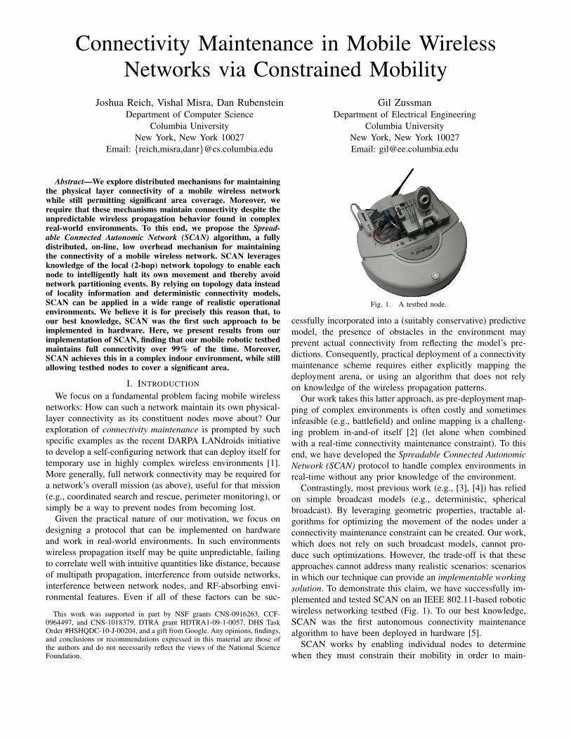
Fig. 1. A testbed node.

cessfully incorporated into a (suitably conservative) predictivemodel, the presence of obstacles in the environment mayprevent actual connectivity from reflecting the model’s pre-dictions. Consequently, practical deployment of a connectivitymaintenance scheme requires either explicitly mapping thedeployment arena, or using an algorithm that does not relyon knowledge of the wireless propagation patterns.

Our work takes this latter approach, as pre-deployment map-ping of complex environments is often costly and sometimesinfeasible (e.g., battlefield) and online mapping is a challeng-ing problem in-and-of itself [2] (let alone when combinedwith a real-time connectivity maintenance constraint). To thisend, we have developed the Spreadable Connected Autonomic

Network (SCAN) protocol to handle complex environments inreal-time without any prior knowledge of the environment.

Contrastingly, most previous work (e.g., [3], [4]) has reliedon simple broadcast models (e.g., deterministic, sphericalbroadcast). By leveraging geometric properties, tractable al-gorithms for optimizing the movement of the nodes under aconnectivity maintenance constraint can be created. Our work,which does not rely on such broadcast models, cannot pro-duce such optimizations. However, the trade-off is that theseapproaches cannot address many realistic scenarios: scenariosin which our technique can provide an implementable working

solution. To demonstrate this claim, we have successfully im-plemented and tested SCAN on an IEEE 802.11-based roboticwireless networking testbed (Fig. 1). To our best knowledge,SCAN was the first autonomous connectivity maintenancealgorithm to have been deployed in hardware [5].

SCAN works by enabling individual nodes to determinewhen they must constrain their mobility in order to main-

tain connectivity. SCAN achieves this through an entirelydistributed process in which individual nodes utilize onlylocal knowledge (2-hop) of the network’s topology to freeze

their movement if SCAN’s decision criterion indicates furthermovement risks network partition. Keeping with our focuson implementability we have designed SCAN to work withcommercially available off-the-shelf components. We havealso designed SCAN to be essentially agnostic to the particularmovement goals of the nodes, allowing SCAN to accommo-date differing mission goals. For example, a civilian self-deploying network might aim to maximize coverage area,while a military version may need to balance coverage withproviding nodes the ability to move when threatened.

Ideally we would desire to assess our mechanism forconnectivity maintenance with respect to how well it providessufficient flexibility to the network to fulfill that network’sparticular objective. As these nuances are difficult to capturewith a straightforward metric (and hence equally difficultto use as an objective function to be optimized), we assessthe performance of our connectivity maintenance mechanismby measuring the coverage area it allows while maintainingconnectivity with bounded probability. We believe this metricoffers a good first-order proxy for our more intuitive but lessprecise criterion.

While SCAN is only a first step towards a comprehensivesolution to an extremely complex and exciting problem, webelieve it offers the correct jumping-off point for futureresearch on practical methodologies for connectivity mainte-nance. Moreover, where previously discussed techniques areapplicable, SCAN offers a robust fall-back mechanism, whileadditionally addressing scenarios in which connectivity of verysimple nodes is desired (e.g., micro-scale robots).

Our main contributions are:• We propose SCAN as a baseline connectivity mainte-

nance mechanism for challenging environments.• We describe SCAN’s intuition and properties under the

most general (and challenged) settings. We also showhow additional specialized information (e.g., RSSI) canbe incorporated into SCAN’s framework (Sec. IV).

• Through analysis and simulation, we evaluate SCAN’sability to maintain network connectivity while enablingsignificant area-coverage. We identify a phase-transitionpoint at which SCAN networks transition betweenasymptotically frozen and always moving, characterizingthat point as a function of the number of nodes andbounding region’s size.

• Finally, we implement SCAN on our mobile roboticnetwork testbed as proof-of-concept, and evaluate itsperformance in providing client coverage (Sec. V).

II. RELATED WORK

Connectivity maintenance for mobile networks has becomean active area of research over the past several years. Thecontrol theory community began to explore this area first, inthe context of motion planning algorithms. In this context,the problems of maximizing some specific target function

and maintaining connectivity are solved jointly. Node move-ment patterns are determined completely by the specifiedcontroller(s). Early work focused on maximal coverage [6] andshortly thereafter on continuously connected group movement[3]. A series of papers considers the use of potential fields tosupply centralized [7], distributed [8], and centralized doubleintegrator [4] schemes for ensuring connectivity while max-imizing a metric encoded in those fields. More recently, [9]adds the consideration of collision avoidance, and [10] looksat the looser constraint that connectivity reoccur periodically.While most work in this area leverages either geometricproperties or assumes perfect knowledge of the potential fieldsused for determining connectivity and utility, in an approachmore closely related to our own, [11] uses only two-hopinformation to maintain connectivity, albeit by dividing thenode population into backbone and regular nodes.

However, all of the above approaches make restrictiveassumptions regarding node connectivity - assumptions whichare unlikely to be true in practice. By far the most popularsuch assumption is that node broadcast ranges are perfectlyspherical, deterministic, non-interfering, and not subject toattenuation from obstacles or other environmental conditions.Notably, [12] does relax these assumptions, considering afairly realistic broadcast model. However, this is done at thecost of only being able to consider simple chain topologies.Given this, it is perhaps unsurprising that only a single,preliminary hardware evaluation of a technique from this bodyof research has been done [13]. Moreover as noted in [13],the evaluation presented could not accommodate cluttered orcomplex environments (the experiment being conducted in asingle, rectangular empty room).

Recently several pieces of work have noted the practicalshortcomings of approaches reliant on unrealistically simplebroadcast assumptions and have taken heuristic approachesutilizing actual connectivity/signal strength information. Con-sequently, these approaches have been much more amenableto at least limited hardware prototyping and evaluation. Previ-ously generated radio signal strength maps and hand-producedfree space cell decompositions, are used by [14] as inputto their connectivity algorithm. A different problem, extend-ing a connected network by having human operators drop“breadcrumb” routers when connectivity begins to weaken,is addressed by [15]. [16] examines mechanisms that repairdisconnected networks, leveraging graph properties similar tothose used by SCAN. Finally, [17] is the work most similar toour own, developing a distributed algorithm that is a slightmodification of the Neighbor Density (ND) algorithm wepresented previously in [5] and use for comparison here. It isshown in [17] that asymptotically this algorithm will producea connected network when run in a bounded space. Whenevaluating this algorithm on a testbed built along the linespublished in [18], [17] found eight nodes needed 35 minutesto converge - several times longer than needed by SCAN asdescribed in V-B.

Finally, it is worth noting that, like the body of workabove, SCAN does not provide a facility for IP-level routing.

We believe most MANET routing protocols should be ableto work alongside the SCAN protocol. However, we note[19] has found that even such protocols may perform poorlywith mobile robots. Consequently we recommend choosing aprotocol that fits well with the SCAN approach, localizingcontrol messages as much as possible to the vicinity oftopological changes.

III. PROBLEM SETTING

A. Operational Environment and Testbed

SCAN was designed to operate in unknown and complexenvironments using commercially available hardware. As aresult, SCAN must contend with unpredictable channel char-acteristics and unknown obstacles to both wireless broadcastand nodal movement. With respect to the former, wirelessbroadcast in the 802.11 spectrum is unpredictable, subject tocross-talk, multipath, fading, and interference. These effectsare only exacerbated by unknown features of the operationalenvironment. Multipath effects are engendered by walls andobstacles, while fading increases in the presence of RF-absorbent surfaces. In such an environment, knowing wheretwo nodes are positioned with respect to one another is oftena very different matter than knowing if they will be wirelesslyconnected. Moreover, many environments are GPS denied andwhile there are techniques addressing indoor localization [20],[21], such systems require significant time to setup and/orleverage expensive hardware.

Automated techniques to create maps that allow such infer-ence to be performed with reasonable confidence are just nowbeing developed [2] and it is unclear if/how these might beincorporated into an algorithm that maps while simultaneouslymaintaining connectivity. Moreover, such a map can quicklybecome obsolete should any contributing factor of the envi-ronment change sufficiently. Our guiding philosophy behindSCAN is that the most effective and practical measure ofwhether nodes will be connected in the future is their current

connectivity. Sec. V-A discusses the features of the particularoperational environment used for our experiments.

We implemented and tested SCAN on our MADNeT mobilerobotic networking testbed, described in [18]. Each mobilenode in our testbed comprises a Linksys WRTSL54GS wire-less router running a build of OpenWrt Linux affixed to aniRobot Roomba Create mobility and sensing platform (Fig. 1).The WRTSL54GS provides communication, computation andmemory, while the Roomba provides power, movement, andenvironmental sensing. Our nodes do not utilize GPS, althoughwe are working to incorporate RSSI (Sec. IV-E). This setup al-lows us to experiment with real mobile nodes whose broadcastand mobility decisions we can specify utilizing standardizedprogramming languages.B. Node Mobility Pattern

Aside from sometimes requiring the Roombas to freeze, weplace no other explicit restrictions on their movement. As ourprimary interest lies in networking, rather than robotics, wehave focused our main efforts on SCAN. To spread our nodesacross the test area we use a simple movement algorithm. Each

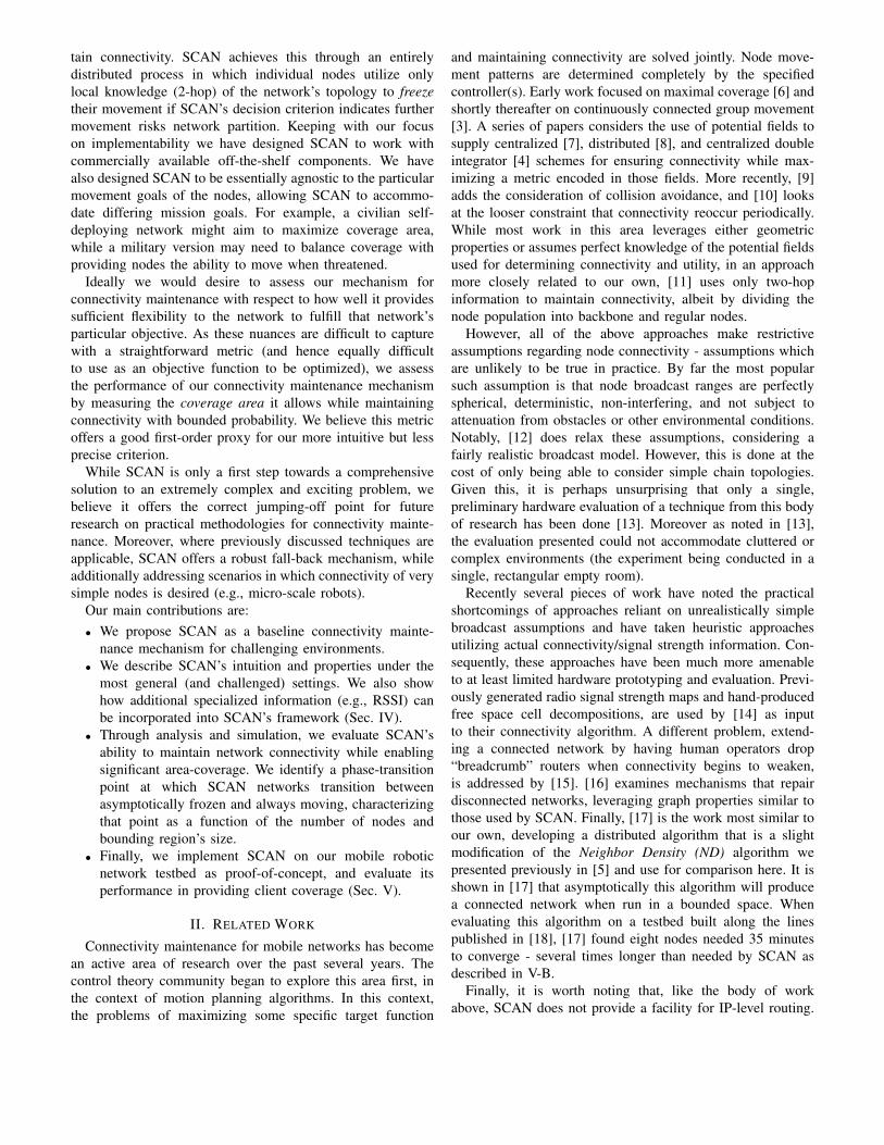
(a) a and b are neighbors. a and dare connected by path (a, b, c, d).

(b) A network with both robust andfragile connections.

Fig. 2. Network connectivity and robustness.

robot moves straight ahead until it is stopped by an obstacle.Each robot has two sensors which allow it to determinewhether the obstacle is off to the side or in front. If the obstacleis to a side, the robot rotates a random angle and continues.If the obstacle is in front, the robot backs up slightly, rotatesa random angle, and proceeds. The important point is that thedefault node movement pattern is oblivious to any networkconnectivity requirement. Consequently, we would believe thatSCAN’s success, at maintaining connectivity while providingfor reasonable area coverage under this movement pattern,generalizes well to many other movement patterns.C. Network Model

Assume our network contains N mobile robots, each witha (mean) transmission range r, and is deployed in an areaA. We represent the network as a graph in which eachnode corresponds to a mobile robot. Two nodes u and vare neighbors and are directly connected via a link, if theycan directly, mutually, and consistently communicate over awireless channel (if u can receive v’s broadcast but not viceversa then u and v are not directly connected).

We define N(u) as the set of nodes that are node u’sneighbors with u /∈ N(u), and assume, as is the case in ourtestbed, that each node u knows N(u), and is also informedof N(v) for each of its neighbors v ∈ N(u). u and v areconnected if there is a path from u to v across a series oflinks. A network is globally connected when every two nodesu and v in the network are connected.

Within each fixed-length assessment period, each nodeassesses its current local connectivity, and, based on this statedecides to either move or freeze until its next assessment. Wedo not require that nodes make their assessments simultane-ously, nor do their respective T ’s need to match exactly (clockdrift is permissible).

Over time, new links can form and existing links can fail.However, the state of a link between two nodes u and vcan change only if at least one of the nodes is moving. Ifboth u and v are frozen, then an existing link between themcannot fail, nor can a link be added when there is none. Inother words, only the mobility of node pairs significantly alterswhether a pair can communicate.

IV. ALGORITHMS FOR CONNECTIVITY MAINTENANCE

Our goal is to develop and evaluate a basic mechanismthat intelligently leverages knowledge of current networkconnectivity characteristics to assess the robustness of currentnetwork connectivity. This assessment is then used to de-termine whether further movement endangers future networkconnectivity. If so, we require that the node(s) for whomthis is true refrain from further movement by freezing until

such time as continued movement no longer poses this risk.To this end we will introduce two algorithms leveraging thisbasic mechanism: a naive Neighbor Density (ND) algorithmwhich uses a very simple metric for assessing connectivityrobustness, and SCAN which conducts a still simple, yetsignificantly more powerful assessment of robustness.

Both ND and SCAN share the common assumption that,while the quality of the wireless channel may fluctuateunpredictably over space, it will remain relatively constantover time: relative movement of two nodes may effect theirconnectivity, but time-wise fluctuations will not have a sig-nificant effect. In situations where the quality of the wirelesschannel is fluctuating wildly over time (e.g., significant andvarying external interference, fast fading) more specialized orconservative techniques will be required.A. Neighbor Density Algorithm

The Neighbor-Density (ND) algorithm (shown in Fig. 3(a))serves as a naive parameterizable heuristic solution to theconnectivity problem. ND utilizes nodal density (or moreprecisely valence) to achieve connectivity: if a node has morethan k neighbors it considers local connectivity robust andconsequently may move, fewer it must freeze. Both [15], [17]use slight variations on ND for maintaining connectivity. ND’smessages are constant in the number of neighbors, as only thesending node’s ID need be sent.B. Spreadable Connected Autonomic Network Algorithm

The Spreadable Connected Autonomic Network (SCAN)

algorithm (shown in Fig. 3(b)) takes the greedy approachthat a node’s movement should only be constrained in directresponse to a perceived lack of robustness in the (local)network connectivity structure. To get a feel for when we maywish to freeze a node, consider the example in Fig. 2(b).

Node a is connected to 3 neighbors. To disconnect a fromany of the neighbors to its right (or in fact any of the nodes towhich it is connected) at least 2 links in S must be broken. Incontrast, only a single link needs to fail to disconnect node afrom node b. When links fail infrequently (e.g., 1 failure duringa assessment period), then if a were only concerned aboutthe nodes in the set S, it could continue to move. However,there is a high likelihood that any movement could cause thesingle link between a and b to fail, ending the connectionwith b, thereby partitioning the network. To keep the networkpartition-free, both a and b should freeze.

But what if, during a assessment period, k ≥ 1 links can beexpected to fail? How do we then determine whether nodesmust freeze to ensure network connectivity is maintained? Itis this question that SCAN is designed to address.

Formally, SCAN is pre-configured with a parameter k, suchthat a node u is allowed to move as long as |N(u)∩N(v)| ≥ kfor every v ∈ N(u). In other words, u moves if it shares kneighbors with each of its neighbors v. If this property doesnot hold for even a single neighbor, u must freeze.

SCAN does require more messaging overhead than ND.SCAN’s messages are linear in the number of neighbors, sincethe sending node must send its own ID and all those of itsneighbors. In practice however, if density is high enough that

this should become an issue, the probability of disconnectionbecomes very low. A practical implementation could switchover to ND until density falls.C. Global Connectivity

Consequently, if a pair of nodes who are connected do havesufficient redundancy in that connection (as routed throughmutual one-hop neighbors), SCAN concludes that movementon either of their part may in the worst case sever all knownlocal routes between these two nodes. Other longer routesmay in fact exist should all local paths be severed, in whichcase these nodes might still remain connected, but SCANconservatively assumes that only known connections can berelied upon in assessing connectivity robustness. By assessingconnectivity robustness between each pair of nodes on a localbasis, we argue (informally) that SCAN prevents any pairof directly connected nodes from severing all of the locallyknown paths between them, and transitively prevents globalnetwork partition.

While we lack space here to make this argument rigorous,we refer the interested reader to our tech report [5] whichproves SCAN’s global connectivity property and shows thatfor any node to be disconnected from a SCAN network atleast k + 1 local link failures must occur within one SCANassessment period.D. Choosing SCAN’s k Parameter

Since SCAN disconnections only occur when at least k +1nearby links fail simultaneously, the best value of k dependsupon how many neighboring links are expected to fail (i.e.,nodes move out of communication range) within a assessmentperiod. As one increases the speed of a node, decreases therange of transmission, or increases the broadcast cycle time,a larger k is needed to ensure connectivity. In general, as kincreases, it becomes less likely that the network will partition,but the expected time that nodes spend moving is reducedas well, which can delay achievement of the goal for whichmobility of nodes is required in the first place. In Section VIwe find that for network whose nodes move slowly k = 2 ismore than sufficient while for more volatile settings k > 4appears extremely robust.

Pre-determining the optimal k for an arbitrary setting isquite hard because: (i) link failures will often exhibit co-dependence, (ii) disconnection of a nearby nodes are de-pendent, (iii) k + 1 nearby link failures permit but do not

necessitate severing of all locally known paths between twoneighbors, and (iv) even if all locally known paths connectinga node to some neighbor are severed, there may still be aglobal path connecting them.

Consequently, we will use a back-of-the-envelope calcu-lation to give some insight into how k should be set. Webegin by setting the probability p of a link breaking during agiven SCAN assessment period to the distance a node travelsin a period divided by the mean broadcast radius. Roughlyspeaking, k + 1 or more links break with probability orderpk+1. Assuming a disconnection lasts for a mean time of τassessment periods, the expected fraction of time the networkis fully connected is 1 − τpk+1. k should be chosen such

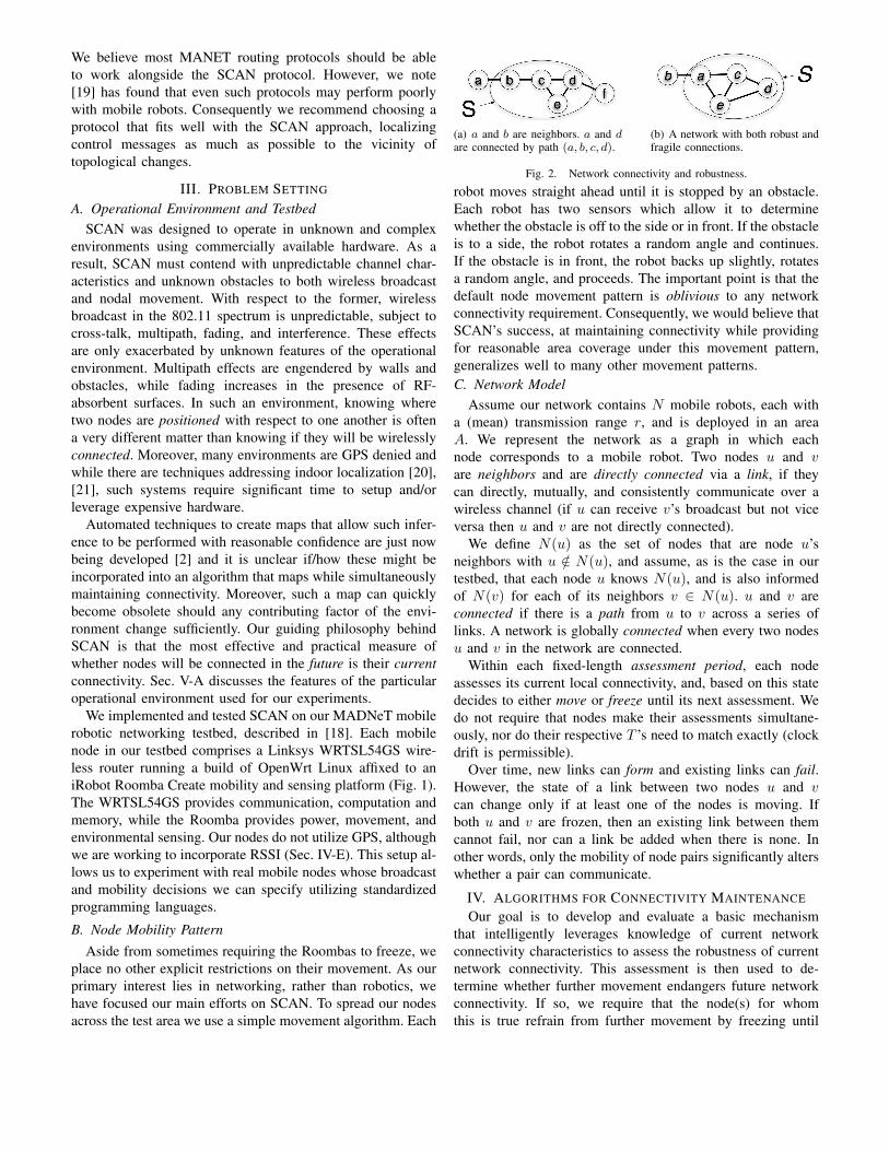
if |N(u)| ≥ k then move else freeze(a) ND

if |N(u) ∩N(v)| ≥ k, ∀v ∈ N(u) then move else freeze(b) SCANFig. 3. Mobility criteria.

that τpk+1 is less than the tolerated level of partitioning. Theinterested reader may observe our algorithm in action and testthe effect of changing k using a simplified applet version ofour simulation environment [22].E. Incorporating Additional Information

While we do not address utilizing additional sources ofinformation such as GPS or RSSI in this paper, we do wishto briefly describe how they might be incorporated in SCAN’sgeneral approach. SCAN simply views each connection as abinary value, 1 if connected, 0 if not, corresponding to thepresence or absence of an edge in our network. A versionof SCAN utilizing additional information (SCAN+) coulduse weighted edges, whose weights correspond to normalizedRSSI values or relative distance measurements. One possibilitywould be to require that the weighted sum of the of the pathsconnecting any neighbor and a given node be greater thana constant k� allowing the presence of strong connections tooffset lower absolute numbers of common neighbors. Clearlymore sophisticated schemes could also be devised leverage anincreasingly nuanced view of the connectivity topology forimproved performance. We leave these for future work.

V. TESTBED EXPERIMENTS

Our was to develop connectivity maintenance techniquesthat could actually be implemented and tested on hardwarein a noisy, challenging environment. To this end, we haveimplemented SCAN on our Roomba robotic testbed and runseveral hours of experiments. This allowed us to validate ourideas in a practical setting and demonstrate SCAN’s efficacyin maintaining the connectivity of a self-deploying mobilenetwork. Recall from Sec. III-B that our nodes operated ina GPS-denied environment and explored the area randomly.Clearly, if our blindly moving nodes could stumble into asuccessful configuration, nodes with more robust mobilityroutines tailored for a particular application could do at leastas well.

We found that SCAN could provide connectivity in aremarkably robust fashion while also providing latitude ofmovement sufficient to cover clients scattered throughout ourtest environment. Out of 273 minutes and 50 seconds ofexperiments, our network remained connected in all but 2minutes and 23 seconds. Moreover, the network partitions weencountered were comprised of one node disconnecting, withthe sole exception of a 15 second period during which a pairof nodes partitioned themselves as a connected component.A. Experimental Setup

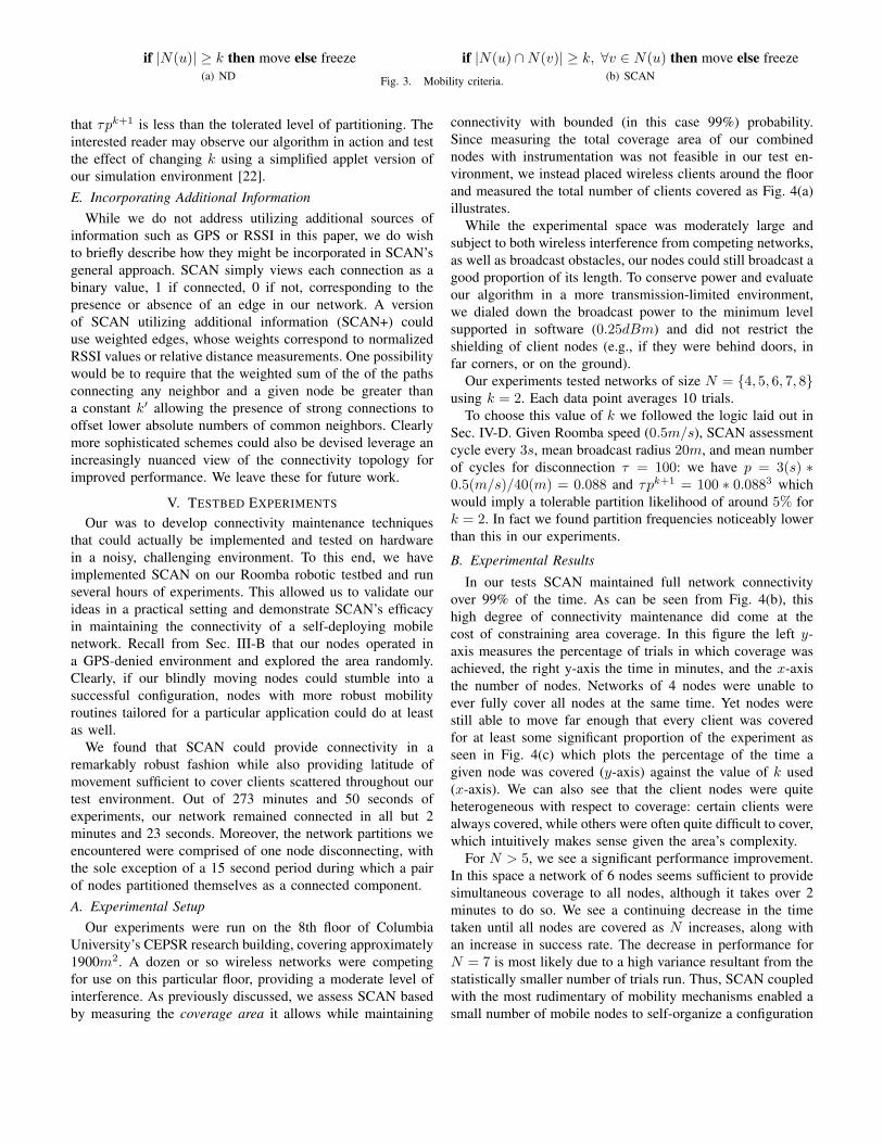
Our experiments were run on the 8th floor of ColumbiaUniversity’s CEPSR research building, covering approximately1900m2. A dozen or so wireless networks were competingfor use on this particular floor, providing a moderate level ofinterference. As previously discussed, we assess SCAN basedby measuring the coverage area it allows while maintaining

connectivity with bounded (in this case 99%) probability.Since measuring the total coverage area of our combinednodes with instrumentation was not feasible in our test en-vironment, we instead placed wireless clients around the floorand measured the total number of clients covered as Fig. 4(a)illustrates.

While the experimental space was moderately large andsubject to both wireless interference from competing networks,as well as broadcast obstacles, our nodes could still broadcast agood proportion of its length. To conserve power and evaluateour algorithm in a more transmission-limited environment,we dialed down the broadcast power to the minimum levelsupported in software (0.25dBm) and did not restrict theshielding of client nodes (e.g., if they were behind doors, infar corners, or on the ground).

Our experiments tested networks of size N = {4, 5, 6, 7, 8}using k = 2. Each data point averages 10 trials.

To choose this value of k we followed the logic laid out inSec. IV-D. Given Roomba speed (0.5m/s), SCAN assessmentcycle every 3s, mean broadcast radius 20m, and mean numberof cycles for disconnection τ = 100: we have p = 3(s) ∗0.5(m/s)/40(m) = 0.088 and τpk+1 = 100 ∗ 0.0883 whichwould imply a tolerable partition likelihood of around 5% fork = 2. In fact we found partition frequencies noticeably lowerthan this in our experiments.

B. Experimental Results

In our tests SCAN maintained full network connectivityover 99% of the time. As can be seen from Fig. 4(b), thishigh degree of connectivity maintenance did come at thecost of constraining area coverage. In this figure the left y-axis measures the percentage of trials in which coverage wasachieved, the right y-axis the time in minutes, and the x-axisthe number of nodes. Networks of 4 nodes were unable toever fully cover all nodes at the same time. Yet nodes werestill able to move far enough that every client was coveredfor at least some significant proportion of the experiment asseen in Fig. 4(c) which plots the percentage of the time agiven node was covered (y-axis) against the value of k used(x-axis). We can also see that the client nodes were quiteheterogeneous with respect to coverage: certain clients werealways covered, while others were often quite difficult to cover,which intuitively makes sense given the area’s complexity.

For N > 5, we see a significant performance improvement.In this space a network of 6 nodes seems sufficient to providesimultaneous coverage to all nodes, although it takes over 2minutes to do so. We see a continuing decrease in the timetaken until all nodes are covered as N increases, along withan increase in success rate. The decrease in performance forN = 7 is most likely due to a high variance resultant from thestatistically smaller number of trials run. Thus, SCAN coupledwith the most rudimentary of mobility mechanisms enabled asmall number of mobile nodes to self-organize a configuration

(a) Indoor space/clients used for experiments.

20

30

40

50

60

70

80

90

100

4 5 6 7 8 1.25

1.5

1.75

2

2.25

2.5

2.75

% T

rial

s A

ll C

lien

ts C

ov

ered

Tim

e

Number of Nodes (N)

% Trials All Clients Covered

Experiment Length

(b) % Trials coverage achieved/time taken. (c) Fraction of time clients were covered.Fig. 4. Testbed experiment results.

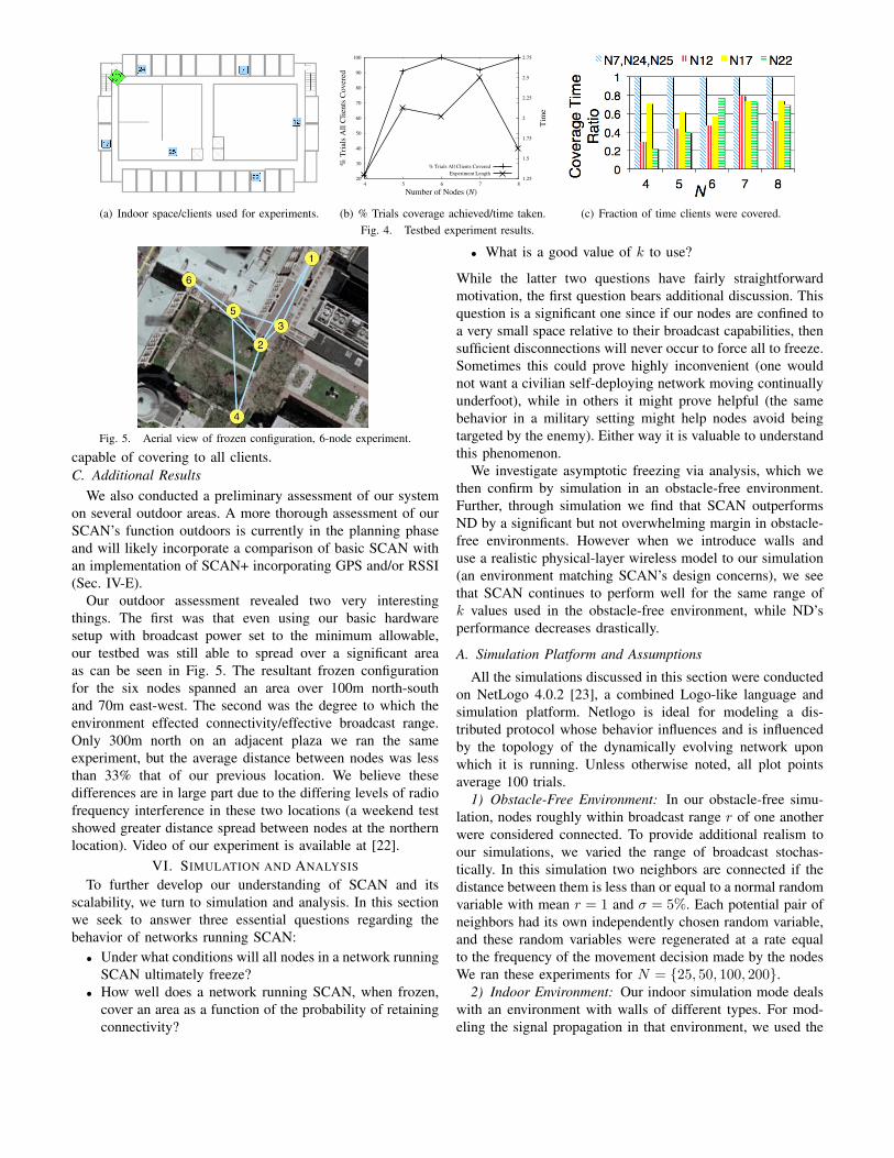
Fig. 5. Aerial view of frozen configuration, 6-node experiment.

capable of covering to all clients.C. Additional Results

We also conducted a preliminary assessment of our systemon several outdoor areas. A more thorough assessment of ourSCAN’s function outdoors is currently in the planning phaseand will likely incorporate a comparison of basic SCAN withan implementation of SCAN+ incorporating GPS and/or RSSI(Sec. IV-E).

Our outdoor assessment revealed two very interestingthings. The first was that even using our basic hardwaresetup with broadcast power set to the minimum allowable,our testbed was still able to spread over a significant areaas can be seen in Fig. 5. The resultant frozen configurationfor the six nodes spanned an area over 100m north-southand 70m east-west. The second was the degree to which theenvironment effected connectivity/effective broadcast range.Only 300m north on an adjacent plaza we ran the sameexperiment, but the average distance between nodes was lessthan 33% that of our previous location. We believe thesedifferences are in large part due to the differing levels of radiofrequency interference in these two locations (a weekend testshowed greater distance spread between nodes at the northernlocation). Video of our experiment is available at [22].

VI. SIMULATION AND ANALYSIS

To further develop our understanding of SCAN and itsscalability, we turn to simulation and analysis. In this sectionwe seek to answer three essential questions regarding thebehavior of networks running SCAN:

• Under what conditions will all nodes in a network runningSCAN ultimately freeze?

• How well does a network running SCAN, when frozen,cover an area as a function of the probability of retainingconnectivity?

• What is a good value of k to use?

While the latter two questions have fairly straightforwardmotivation, the first question bears additional discussion. Thisquestion is a significant one since if our nodes are confined toa very small space relative to their broadcast capabilities, thensufficient disconnections will never occur to force all to freeze.Sometimes this could prove highly inconvenient (one wouldnot want a civilian self-deploying network moving continuallyunderfoot), while in others it might prove helpful (the samebehavior in a military setting might help nodes avoid beingtargeted by the enemy). Either way it is valuable to understandthis phenomenon.

We investigate asymptotic freezing via analysis, which wethen confirm by simulation in an obstacle-free environment.Further, through simulation we find that SCAN outperformsND by a significant but not overwhelming margin in obstacle-free environments. However when we introduce walls anduse a realistic physical-layer wireless model to our simulation(an environment matching SCAN’s design concerns), we seethat SCAN continues to perform well for the same range ofk values used in the obstacle-free environment, while ND’sperformance decreases drastically.

A. Simulation Platform and Assumptions

All the simulations discussed in this section were conductedon NetLogo 4.0.2 [23], a combined Logo-like language andsimulation platform. Netlogo is ideal for modeling a dis-tributed protocol whose behavior influences and is influencedby the topology of the dynamically evolving network uponwhich it is running. Unless otherwise noted, all plot pointsaverage 100 trials.

1) Obstacle-Free Environment: In our obstacle-free simu-lation, nodes roughly within broadcast range r of one anotherwere considered connected. To provide additional realism toour simulations, we varied the range of broadcast stochas-tically. In this simulation two neighbors are connected if thedistance between them is less than or equal to a normal randomvariable with mean r = 1 and σ = 5%. Each potential pair ofneighbors had its own independently chosen random variable,and these random variables were regenerated at a rate equalto the frequency of the movement decision made by the nodesWe ran these experiments for N = {25, 50, 100, 200}.

2) Indoor Environment: Our indoor simulation mode dealswith an environment with walls of different types. For mod-eling the signal propagation in that environment, we used the

COST 231 Multi-Wall Model (MWM) [24, Ch. 4]. Among theempirical models, this is one of the most sophisticated onesand it is applicable in the 2.45GHz band. The MWM modelprovides the path loss as the free space loss added with lossesintroduced by the walls and floors penetrated by the direct pathbetween the transmitter and the receiver. Since we consider asingle floor, the loss (in dB) is given by:

L = Lfs + Lc + kw1Lw1 + kw2Lw2 (1)

where Lc is constant loss (we assume Lc = 0), kw1 is thenumber of light walls, Lw1 = 3.4dB is the loss due to a lightwall, kw2 is the number of heavy walls, Lw1 = 6.9dB is theloss due to a heavy wall, and Lfs is the free space loss givenby

Lfs = 32.4 + 20 log(r/1000) + 20 log(f) (2)

where r is the distance between the transmitter and receiver(in meters) and f is the frequency in MHz (2450 in our case).

As much as possible, we aimed for our simulation to parallelour indoor experiments, using the same set of barriers shown inFig. 4(a) for our indoor simulations. We set the transmit powerof a node to 0dBm (1mW ). We assume that the receiversensitivity is −82dBm, which is a reasonable value for ICE802.11g devices and we assume a fast fading margin of 16dB.Hence, we require that the propagation loss will satisfy 0 −(−82)−L > 16 (or simply L < 66) in order for two nodes tobe within transmission range. In an environment without wallsthis translates to allowed distance of approximately 17m. In amulti-wall environment the distance varies with the locationsof the different nodes.

We note that the simulation model ignores collisions be-tween SCAN messages simultaneously sent by other nodes. Inour actual implementation, messages were sent on the orderof seconds making such collisions very unlikely.

Given the higher computational complexity of these experi-ments our simulations here were done for N = {8, 16, 32, 64}.

3) Link Failure: In either simulation environment, the mainfactor in whether two nodes are connected arises from nodes’mobility. In our analysis, we do not consider stochasticity,relative movement being the only factor in determining con-nectivity. This assumption is made only to ease our analysisand is not needed for SCAN to function correctly, as ourtestbed experiments in Sec. V demonstrate.

B. The Freeze Phase-Transition

If our nodes are confined to a very small space relative totheir transmission radii, then they will never freeze. As thesize of the space is increased, and they are able to spreadfurther apart, the likelihood of freezing increases. As the sizeof the space grows to ∞, we eventually will reach a pointwhere, with probability 1, all nodes will have frozen. At thispoint, since all nodes are frozen, they cannot obtain newneighbors, and the network remains in a frozen configuration.Here, we investigate the point of the phase-transition: for agiven k and N , what is the ratio of the size of the space tothe node transmission radius, beneath which the network isforever moving, and above which the network always reaches

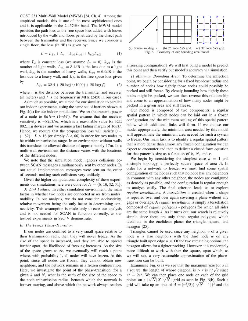
(a) Square w/ diag. r. (b) 25 node 5x5 grid. (c) 37 node 5x5 grid.Fig. 6. Geometry of our bounding area model.

a freezing configuration? We will first build a model to predictthis point and then verify our model’s accuracy via simulation.

1) Minimum Bounding Area: To determine the inflectionpoint, we begin by considering for a fixed broadcast radius andnumber of nodes how tightly those nodes could possibly bepacked and still freeze. By closely bounding how tightly thesenodes might be packed, we can then reverse this relationshipand come to an approximation of how many nodes might bepacked in a given area and still freeze.

Our model is composed of two components: a regularspatial pattern in which nodes can be laid out in a frozenconfiguration and the minimum scaling of this spatial patternbelow which additional links will form. If we choose ourmodel appropriately, the minimum area needed by this modelwill approximate the minimum area needed for such a systemto freeze. Our main task is to identify a regular spatial patternthat is more dense than almost any frozen configuration we canexpect to encounter and then to deliver a closed form equationfor that pattern’s size as a function of k, N , and r.

We begin by considering the simplest case k = 1 anda simple topology, a perfectly square space of area A. Inorder for a network to freeze, we must find some spatialconfiguration of the nodes such that no node has any neighborsin common with any other neighbor, the nodes are configuredas densely as possible, and the configuration is regular enoughto analyze easily. The final criterion leads us to exploreregular tessellations. A tessellation is created when a shapeis repeated over and over again covering a plane without anygaps or overlaps. A regular tessellation is simply a tessellationcomposed of regular polygons - polygons for which all sidesare the same length s. As it turns out, our search is relativelysimple since there are only three regular polygons whichtessellate in the euclidean plane: the triangle, square, andhexagon [25].

Triangles cannot be used since any neighbor v of a givennode u is also neighbors with the third node w on anytriangle built upon edge u, v. Of the two remaining options, thehexagon allows for a tighter packing. However, it is moderatelymore difficult to work with than the square, upon which, aswe will see, a very reasonable approximation of the phase-transition can be built.

Examining Fig. 6(a) we see that the maximum size for s ina square, the length of whose diagonal is > r is r/

√2 since

r2 = 2s2. We can then place one node on each of the gridpoints on a �

√N�X�

√N� grid as seen in Fig. 6(b). Such a

grid will take up an area of A = (r2/2)(�√

N − 1�)2 and the

ratio of one node’s broadcast to the N-node bounding area is

πr2/A = 2π(�√

N� − 1)2 (3)

Extending this model to cover larger k is not overly difficult.For k = 2 instead of placing a single node at each gridintersection, we place two nodes at every other intersectionas seen in Fig. 6(c). In this way, each node shares preciselyone node with any of its neighbors, whether it is alone on itsgrid point or sharing it. Then, for a given N we only need��

2N/3� − 1 grid lines on each side, requiring an area of(r2/2)(�

�2N/3� − 1)2. k = 3 is even easier requiring us to

put two nodes at each grid intersection. We can extend thisstrategy to arbitrary k ≥ 1 obtaining:

πr2/A = 2π/(��

2N/(k + 1)� − 1)2 (4)

which describes the ratio of an individual node’s broadcastarea to the total area. As will now be seen, our model’sprediction tightly bounds the behavior seen in simulation.

2) Ratio of Broadcast Area to Bounding Area in Simula-

tion: Our simulation results in this section were obtainedthrough a binary search for the largest ratio of individual nodebroadcast area to bounding area that would result in a frozenconfiguration. The precise phase-transition point is difficultto determine via simulation (since showing the hypotheticaltransition value fails to ever freeze would require infinitetime). Instead, we estimate this value by measuring the averageconvergence times from our experiments in the unboundedspace and allowed our system to run in excess of 10 times themaximum convergence times taken there.

Each combination of N and k received 10 trials, eachover the course of up to 5000 time-steps. To obtain a clearercorrespondence with our model, in this trial alone we did notstochastically vary the connection lengths. At the end of eachtrial that did not result in a freezing configuration, the ratiowas decreased by half its current value for the subsequent trial.Conversely, whenever a trial ended in a freezing configurationthe ratio would be increased by half. The first trial began witha ratio above the point where freezing could occur, but not toofar. This was determined by a set of preliminary experiments.

The results of our exploration for k = 1, 4 are shown inFig. 7(a), as are the model predictions from (4) (other k valuesbound similarly but were omitted for graphical clarity). In thisfigure the y-axis measures the ratio of an individual node’sbroadcast area to the total bounding area while the x-axismeasures the number of nodes N , each plot point representingthe highest such ratio found at which a network of N froze.

The behavior of the phase-transition point for all k can becharacterized roughly as for every doubling in the number ofnodes, the ratio between node broadcast area and boundingarea decreases by slightly less than half. Moreover, increasingvalues of k appear to lie at a relatively constant log-scaledistance above one another. This is unsurprising as at higherlevels of k a given number of nodes with a given broadcastarea can fit into a smaller bounding space while still beingable to reach a freezing state as argued in our model above.

C. Performance in Obstacle-Free Environments

Here, we explore properties of the frozen configurationwhen SCAN and ND are applied in an unbounded space,where the configuration is guaranteed to eventually freeze. Inour simulation, nodes are deployed at a gateway from whichthey proceed to spread across a 2-dimensional plane. As thesenodes spread across the plane, they extend the area whichthe network attached to the station covers. However, if nodesbecomes cut-off from the gateway through a network partitionevent, the entire area over which only these nodes broadcastceases to be covered. Here we measure coverage area as theunion of the area over which nodes currently connected tothe gateway can broadcast. Consequently, coverage implicitlytakes into account global connectivity, insofar as that connec-tivity benefits the coverage goal of a self-deploying wirelessnetwork.

Fig. 7(b) plots the size of SCAN’s coverage area (y-axis) asa function of k (x-axis). The different curves depict differingnumbers of nodes in the network, with each node’s commu-nication range averaging a unit distance. Not surprisingly, thecoverage area increases in proportion to the size of N , and isa decreasing convex function with the size of k, where nodesare required to maintain larger collections of neighbor sets.Additionally, it is worth noting that for k = 1 the benefit ofincreased mobility in providing greater coverage is more thanoffset by the decrease in connectivity. While for k > 2, thefrequency of any network partition does decrease but provesincreasingly costly from a coverage standpoint.

Fig 7(c) provides a comparable plot for ND. The sametrends discussed for SCAN are apparent, although optimallyparametrized SCAN covers in excess of 50% greater area thanoptimally parametrized ND.

We lack the space for an in-depth investigation of connec-tivity and partition rate as a secondary phenomenon separatefrom coverage. For such an investigation see [5].D. Performance in Indoor Environments

In this set of simulation experiments we examined howSCAN and ND performed in a more complex environment,filled with walls that were obstacles to both wireless signalpropagation and also to node movement. For SCAN wefound the relationship between k and the coverage area to besubstantially similar to those of the obstacle-free environment,albeit with slightly higher rates of partition for a given k.However, things are very different for the parametrization ofND. In an indoor environment the presence of walls affects notonly connectivity but also movement. Indoors, corridors andother obstacles increase the likelihood that a cluster of nodesbegins moving in the same direction. When this occurs ND’sbehavior becomes pathological. Particularly if the number ofnodes in the cluster is greater than k, then all nodes in thecluster will be able to move away from the rest of the networkwithout ND’s freezing criterion being triggered. Thus k mustbe made very high in order to maintain connectivity.

Partially as a consequence of this, partially because SCAN’sfunctioning is little affected by obstacles, the difference inperformance between them is significantly greater than in

(a) Freezing phase transition. (b) Attained coverage, SCAN. (c) Attained coverage, ND. (d) Indoor, 32 nodes.Fig. 7. Simulation results.

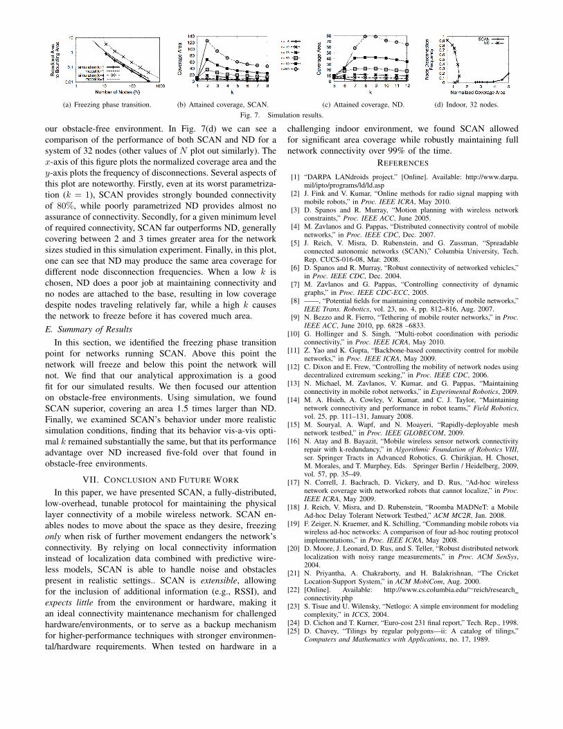
our obstacle-free environment. In Fig. 7(d) we can see acomparison of the performance of both SCAN and ND for asystem of 32 nodes (other values of N plot out similarly). Thex-axis of this figure plots the normalized coverage area and they-axis plots the frequency of disconnections. Several aspects ofthis plot are noteworthy. Firstly, even at its worst parametriza-tion (k = 1), SCAN provides strongly bounded connectivityof 80%, while poorly parametrized ND provides almost noassurance of connectivity. Secondly, for a given minimum levelof required connectivity, SCAN far outperforms ND, generallycovering between 2 and 3 times greater area for the networksizes studied in this simulation experiment. Finally, in this plot,one can see that ND may produce the same area coverage fordifferent node disconnection frequencies. When a low k ischosen, ND does a poor job at maintaining connectivity andno nodes are attached to the base, resulting in low coveragedespite nodes traveling relatively far, while a high k causesthe network to freeze before it has covered much area.E. Summary of Results

In this section, we identified the freezing phase transitionpoint for networks running SCAN. Above this point thenetwork will freeze and below this point the network willnot. We find that our analytical approximation is a goodfit for our simulated results. We then focused our attentionon obstacle-free environments. Using simulation, we foundSCAN superior, covering an area 1.5 times larger than ND.Finally, we examined SCAN’s behavior under more realisticsimulation conditions, finding that its behavior vis-a-vis opti-mal k remained substantially the same, but that its performanceadvantage over ND increased five-fold over that found inobstacle-free environments.

VII. CONCLUSION AND FUTURE WORK

In this paper, we have presented SCAN, a fully-distributed,low-overhead, tunable protocol for maintaining the physicallayer connectivity of a mobile wireless network. SCAN en-ables nodes to move about the space as they desire, freezingonly when risk of further movement endangers the network’sconnectivity. By relying on local connectivity informationinstead of localization data combined with predictive wire-less models, SCAN is able to handle noise and obstaclespresent in realistic settings.. SCAN is extensible, allowingfor the inclusion of additional information (e.g., RSSI), andexpects little from the environment or hardware, making itan ideal connectivity maintenance mechanism for challengedhardware/environments, or to serve as a backup mechanismfor higher-performance techniques with stronger environmen-tal/hardware requirements. When tested on hardware in a

challenging indoor environment, we found SCAN allowedfor significant area coverage while robustly maintaining fullnetwork connectivity over 99% of the time.

REFERENCES

[1] “DARPA LANdroids project.” [Online]. Available: http://www.darpa.mil/ipto/programs/ld/ld.asp

[2] J. Fink and V. Kumar, “Online methods for radio signal mapping withmobile robots,” in Proc. IEEE ICRA, May 2010.

[3] D. Spanos and R. Murray, “Motion planning with wireless networkconstraints,” Proc. IEEE ACC, June 2005.

[4] M. Zavlanos and G. Pappas, “Distributed connectivity control of mobilenetworks,” in Proc. IEEE CDC, Dec. 2007.

[5] J. Reich, V. Misra, D. Rubenstein, and G. Zussman, “Spreadableconnected autonomic networks (SCAN),” Columbia University, Tech.Rep. CUCS-016-08, Mar. 2008.

[6] D. Spanos and R. Murray, “Robust connectivity of networked vehicles,”in Proc. IEEE CDC, Dec. 2004.

[7] M. Zavlanos and G. Pappas, “Controlling connectivity of dynamicgraphs,” in Proc. IEEE CDC-ECC, 2005.

[8] ——, “Potential fields for maintaining connectivity of mobile networks,”IEEE Trans. Robotics, vol. 23, no. 4, pp. 812–816, Aug. 2007.

[9] N. Bezzo and R. Fierro, “Tethering of mobile router networks,” in Proc.

IEEE ACC, June 2010, pp. 6828 –6833.[10] G. Hollinger and S. Singh, “Multi-robot coordination with periodic

connectivity,” in Proc. IEEE ICRA, May 2010.[11] Z. Yao and K. Gupta, “Backbone-based connectivity control for mobile

networks,” in Proc. IEEE ICRA, May 2009.[12] C. Dixon and E. Frew, “Controlling the mobility of network nodes using

decentralized extremum seeking,” in Proc. IEEE CDC, 2006.[13] N. Michael, M. Zavlanos, V. Kumar, and G. Pappas, “Maintaining

connectivity in mobile robot networks,” in Experimental Robotics, 2009.[14] M. A. Hsieh, A. Cowley, V. Kumar, and C. J. Taylor, “Maintaining

network connectivity and performance in robot teams,” Field Robotics,vol. 25, pp. 111–131, January 2008.

[15] M. Souryal, A. Wapf, and N. Moayeri, “Rapidly-deployable meshnetwork testbed,” in Proc. IEEE GLOBECOM, 2009.

[16] N. Atay and B. Bayazit, “Mobile wireless sensor network connectivityrepair with k-redundancy,” in Algorithmic Foundation of Robotics VIII,ser. Springer Tracts in Advanced Robotics, G. Chirikjian, H. Choset,M. Morales, and T. Murphey, Eds. Springer Berlin / Heidelberg, 2009,vol. 57, pp. 35–49.

[17] N. Correll, J. Bachrach, D. Vickery, and D. Rus, “Ad-hoc wirelessnetwork coverage with networked robots that cannot localize,” in Proc.

IEEE ICRA, May 2009.[18] J. Reich, V. Misra, and D. Rubenstein, “Roomba MADNeT: a Mobile

Ad-hoc Delay Tolerant Network Testbed,” ACM MC2R, Jan. 2008.[19] F. Zeiger, N. Kraemer, and K. Schilling, “Commanding mobile robots via

wireless ad-hoc networks: A comparison of four ad-hoc routing protocolimplementations,” in Proc. IEEE ICRA, May 2008.

[20] D. Moore, J. Leonard, D. Rus, and S. Teller, “Robust distributed networklocalization with noisy range measurements,” in Proc. ACM SenSys,2004.

[21] N. Priyantha, A. Chakraborty, and H. Balakrishnan, “The CricketLocation-Support System,” in ACM MobiCom, Aug. 2000.

[22] [Online]. Available: http://www.cs.columbia.edu/∼reich/researchconnectivity.php

[23] S. Tisue and U. Wilensky, “Netlogo: A simple environment for modelingcomplexity,” in ICCS, 2004.

[24] D. Cichon and T. Kurner, “Euro-cost 231 final report,” Tech. Rep., 1998.[25] D. Chavey, “Tilings by regular polygons—ii: A catalog of tilings,”

Computers and Mathematics with Applications, no. 17, 1989.