Connectivity of channelized reservoirs: a modelling approach

David K. Larue1 and Joseph Hovadik2

1ChevronTexaco, Energy Technology Company, Bakersfield, CA, USA2ChevronTexaco, Energy Technology Company, San Ramon, CA, USA

ABSTRACT: Connectivity represents one of the fundamental properties of areservoir that directly affects recovery. If a portion of the reservoir is not connectedto a well, it cannot be drained. Geobody or sandbody connectivity is defined as thepercentage of the reservoir that is connected, and reservoir connectivity is defined asthe percentage of the reservoir that is connected to wells.

Previous studies have mostly considered mathematical, physical and engineeringaspects of connectivity. In the current study, the stratigraphy of connectivity ischaracterized using simple, 3D geostatistical models. Based on these modellingstudies, stratigraphic connectivity is good, usually greater than 90%, if the net: grossratio, or sand fraction, is greater than about 30%. At net: gross values less than 30%,there is a rapid diminishment of connectivity as a function of net: gross. Thisbehaviour between net: gross and connectivity defines a characteristic ‘S-curve’, inwhich the connectivity is high for net: gross values above 30%, then diminishesrapidly and approaches 0.

Well configuration factors that can influence reservoir connectivity are welldensity, well orientation (vertical or horizontal; horizontal parallel to channels orperpendicular) and length of completion zones. Reservoir connectivity as a functionof net: gross can be improved by several factors: presence of overbank sandy facies,deposition of channels in a channel belt, deposition of channels with highwidth/thickness ratios, and deposition of channels during variable floodplainaggradation rates. Connectivity can be reduced substantially in two-dimensionalreservoirs, in map view or in cross-section, by volume support effects and bystratigraphic heterogeneities. It is well known that in two dimensions, the cascadezone for the ‘S-curve’ of net: gross plotted against connectivity occurs at about 60%net: gross. Generalizing this knowledge, any time that a reservoir can be regarded as‘two-dimensional’, connectivity should follow the 2D ‘S-curve’. For channelizedreservoirs in map view, this occurs with straight, parallel channels. This 2D effect canalso occur in layered reservoirs, where thin channelized sheets are separatedvertically by sealing mudstone horizons. Evidence of transitional 2D to 3Dbehaviour is presented in this study. As the gross rock volume of a reservoir isreduced (for example, by fault compartmentalization) relative to the size of thedepositional element (for example, the channel body), there are fewer potentialconnecting pathways. Lack of support volume creates additional uncertainty inconnectivity and may substantially reduce connectivity. Connectivity can also bereduced by continuous mudstone drapes along the base of channel surfaces, bymudstone beds that are continuous within channel deposits, or muddy inclinedheterolithic stratification. Finally, connectivity can be reduced by ‘compensational’stacking of channel deposits, in which channels avoid amalgamating with otherchannel deposits. Other factors have been studied to address impact on connectivity,including modelling program type, presence of shale-filled channels and nestedhierarchical modelling.

Most of the stratigraphic factors that affect reservoir connectivity can beaddressed by careful geological studies of available core, well log and seismicdata. Remaining uncertainty can be addressed by constructing 3D geologicalmodels.

KEYWORDS: reservoir, sequence stratigraphy, connectivity, deep-water channel deposits, turbidites

Petroleum Geoscience, Vol. 12 2006, pp. 291–308 1354-0793/06/$15.00 � 2006 EAGE/Geological Society of London

INTRODUCTION

Reservoir connectivity represents one of the primary controlson recovery from a petroleum reservoir. Reservoir connectivityissues are especially significant in sparse well environments,such as deep water, in which economic limits to drilling wellsexist but questions regarding connectivity pertain. This studyreviews definitions of different types of reservoir connectivityand shows how stratigraphic architecture affects connectivity.Different types of stratigraphic architectures in 3D geostatisticalmodels were created and analysed for connectivity. Thisapproach, while allowing analysis of thousands of differentstratigraphic characterizations, is limited mainly by our ability tocreate realistic reservoir stratigraphy, as well as scaling issuesassociated with using gridded models. Based on the results ofthis study, lists of stratigraphic characteristics that influencereservoir connectivity and techniques for their recognition arepresented.

Vertical compartmentalization of a reservoir can occurwhenever a laterally continuous impermeable unit separates alower from an upper permeable unit. That is, because of theimpermeable unit, pressures in the upper and lower reservoirsprior to, and/or during production may be different. If onlyone of the units is completed in a well, only that reservoirinterval will be drained, and the other reservoir interval willmaintain original pressure and fluid saturation distributions.Based on sequence stratigraphic studies (Van Wagoner et al.1990; Van Wagoner 1995; Larue & Legarre 2004), reservoirs

may become vertically compartmentalized associated withchanges in sea-level, tectonic activity and accompanyingchanges in depositional systems (Fig. 1A).

Lateral compartmentalization of reservoirs, or the arealseparation of reservoir compartments, is the focus of this study.Lateral compartmentalization can occur in several situations. Itis clear that impermeable fault zones (Fig. 1B, ‘sealing fault’) orfaults that emplace impermeable intervals next to permeableintervals (Fig. 1B, ‘non-sealing fault’) cause lateral reservoircompartmentalization. Fault compartmentalization will not bediscussed further here (see Fulljames et al. 1997; Knipe 1997).Lateral compartmentalization of channelized deposits occurswhen individual channel bodies fail to intersect (Fig. 1C) andthere are no permeable conduits connecting channels (forexample, crevasse-splay deposits or overbank sandstones).Factors influencing lateral connectivity of channelized andother reservoirs will be presented, stressing the cases in whichpermeable sandstones are confined to channel deposits, andoverbank deposits are non-permeable mudstones.

Many of the concepts accepted today about connectivity arederived from field-based studies of waterflooding in WestTexas and other fields in the USA (Stiles 1976; George & Stiles1978; Barber et al. 1983; Gould & Sarem 1989; Stiles &Magruder 1992). These studies stressed that unless there wascontinuity between the injecting and producing wells during awaterflood, the reservoir would be incompletely swept. If thereservoir is incompletely swept, infill drilling provides an

Fig. 1. (A) Formation of vertical compartments in a shoreface reservoir associated with progradational cycles and relative changes in sea-level.Wells intersecting four separate vertical compartments are shown. Modified from a figure in Van Wagoner et al. (1990). (B) Lateralcompartmentalization can be accomplished through sealing and non-sealing faults. Connected channel deposits shown in the same colour.Sandstone bodies in contact across the fault are connected in the non-sealing case and unconnected in the sealing case. Two wells are shown.(C) Map view, showing formation of lateral compartments in a channelized reservoir by avulsion. ‘OWC’ is the oil–water contact. Injecting andproducing wells (‘Inj’ and ‘Prod’) are shown for each channel complex. (D) Example of reservoir geobodies, representing individual channeldeposits (yellow), or amalgamated channel deposits (orange). (E) Reservoir connectivity is defined as the proportion of reservoir connected toone or more wells. Here, the orange geobodies are connected elements, while the yellow bodies are unconnected. (F) If producing and injectingwells are present, connectivity can be defined as the percentage of the reservoir geobodies intersected by both injecting and producing wells (theorange channel deposits). Note that other types of connectivity are also defined in this situation, including geobodies in contact only withinjecting or producing wells (pink or blue, respectively) and geobodies unconnected to the wells (yellow). (G) Connectivity can be defined as afunction of the completed interval in the well. Colours as in (E). (H) Connectivity can be defined for non-vertical wells. Colours as in (E).

D. K. Larue & J. Hovadik292

opportunity to both increase the rate of production in the fieldand also to add to reserves (Abbots & van Kuijk 1997).

RECOGNITION OF RESERVOIR COMPARTMENTS

Reservoir compartments are non-connected parts of the reser-voir. They are recognized in fields undergoing developmentbased on interpretation of seismic data, and measurementsfrom wells, including different pressures, pressure gradients, ordifferent fluid contacts (for example, Smalley & Hale 1995;Hardage et al. 1997). Differences in oil geochemistry fromdifferent wells or zones in the well can also lead to interpreta-tions of reservoir compartments (Beeunas et al. 1999; Edman &Burk 1999). In older fields, differences in pressures or changeswith pressure over time may be associated with production, ormay be associated with reservoir compartments. Penetration ofa zone with original pre-production field pressures couldindicate a new compartment unless the field has been under-going pressure maintenance, or has a strong aquifer. In a fieldproduced with a water drive or by waterflooding, original fieldwater saturation values cannot be used as an indicator ofcompartmentalization, because water motions can be complex.Interpretation of 4D seismic data can lead to definition of newreservoir compartments (Anderson et al. 1995). In general,definition of subtle reservoir compartments may not be simpleor straightforward.

SEDIMENTOLOGY AND STRATIGRAPHY OFCONNECTIVITY

Concepts about origins and causes of lateral connectivity ofreservoirs are based on sequence stratigraphic, sedimentologicaland geomorphological studies (for example, Martinsen 1994).During deposition, all channel types, whether fluvial, estuarineor deep water, undergo some degree of migration or shiftingwhich tends to produce channel deposits that are wider andthicker than original channel dimensions (Leeder 1978;Bridge & Leeder 1979; Bridge 1993; Mack & Leeder 1998;Posamentier et al. 2000). Gradual migration and shifting ofchannels with accompanying local events, such as chute andneck cut-off, tends to make channel belt deposits, also referredto as channel family or channel complex deposits (Bridge 1993;Bratvold et al. 1994). The relative sudden movement of thechannel belt to another position in the depositional system istermed avulsion (Smith et al. 1989; Jones & Schumm 1999;Mohrig et al. 2000). Channel deposits that are laterally discon-nected were clearly subjected to either or both gradual migra-tion and avulsive events. An example of channels disconnectedby an avulsion event is shown in Figure 1C. Here, an updipavulsion resulted in the bifurcation of two channel belts. Withinthe oil zone, shown by the oil–water contact, the two channelcomplexes are not in communication, such that there will beminimal communication between the two well pairs shown(there could be some pressure communication due to acommon water leg, however). There are aggradational andsequence stratigraphic components to channel connectivity thatwill be addressed herein, in that channel base-level changes aretied to changes in relative sea-level, climate and tectonics(Shanley & McCabe 1994; Bryant et al. 1995; Van Wagoner1995; Posamentier et al. 2000). Much of the understanding ofchannel migration and avulsion is derived from studies offluvial systems. Although deep-water channel deposits are alsoknown to migrate and aggrade, and avulsions have beendocumented, depositional processes and origins are less wellunderstood (Posamentier et al. 2000; Kolla et al. 2001; Abreuet al. 2003).

TYPES OF CONNECTIVITY

Several types of connectivity between channels or otherdepositional elements can be defined. Geobody or sandbodyconnectivity refers to the connectivity of individual elementsin a reservoir, such as amalgamated channel deposits (Fig. 1D).Connected and unconnected channel deposits define channel-sized or larger potential flow units referred to as geobodies.Geobody connectivity has been studied by a number ofworkers (Allen 1978, 1979; Allard & HERESIM Group 1993;Pardo-Iguzquiza & Dowd 2003).

Reservoir-to-well connectivity, or simply reservoir connec-tivity, is defined as the proportion of the reservoir connected towells (Fig. 1E). Because reservoir connectivity requires infor-mation about the wells, and is unique to their location, reservoirconnectivity is both a well property and a reservoir property.It is a well property because, given one or more wells, theproportion of the reservoir connected to the wells can bedefined and this number is uniquely defined for that well group.Reservoir-to-well connectivity is also a reservoir property inthat it defines which reservoir elements are connected to agiven well or group of wells.

In a field with both producing and injecting wells, reservoirconnectivity can be defined as the proportion of the reservoirconnected to both producing and injecting wells, or to only theproducing or injecting wells (Fig. 1F). Note that reservoirconnectivity is dependent on where the well was perforated orcompleted (Fig. 1G). A technique for searching for connectivityfrom completions is presented by Lo & Chu (1998). In ourstudies, a simpler and faster technique based on intersectionsof geobodies is used. Connectivity can also be defined forhorizontal or deviated wells (Fig. 1H).

CALCULATING CONNECTIVITY IN RESERVOIRCHARACTERIZATIONS

To define connectivity, one or more parameters are definedthat differentiate ability for fluid to flow in the reservoir. Forexample, a permeability, facies, porosity or Vshale cut-off (orcombination of cut-offs) may be applied that differentiatesrocks in which fluids could flow at some geologically reasonablerates from rocks that are essentially impermeable. Time-scale is,of course, important and the cut-offs considered in the oilindustry usually involve time-scales that are compatible withproducing a field, typically 20 years or so. Examples ofpermeability cut-offs might be 0.1 mD or 1 mD for a relativelylight oil, or 10 mD or >100 mD for a heavier oil. In the presentstudy, a facies cut-off is used to define potential flow units.

Once potential flow units are defined based on the userspecified cut-off, a computer program is used to find theconnected cells in the reservoir (Allen 1978; King 1990; Allard& HERESIM Group 1993; Deutsch 1998; Lo & Chu 1998;Pardo-Iguzquiza & Dowd 2003). Groups of connected cells aredefined as geobodies, and geobody connectivity is defined asthe ratio of the volume of the largest geobody to the sum of allthe reservoir geobodies. Then, to define reservoir connectivity,the volume of geobodies intersected by wells is divided by thetotal volume of geobodies.

IMPLICATIONS OF CONNECTIVITY

A tacit implication of these definitions of connectivity is that ifthe reservoir is connected to the well, then the reservoir isproducible. This is a binary or categorical classification of thereservoir and clearly cannot always be the case. In Figure 2A, awell is shown that penetrates a channel deposit. This channeldeposit continues on for a kilometre. It is questionable whether

Modelling the connectivity of channelized reservoirs 293

a single well could drain the mobile fluids in the entire channeldeposit (mobile fluids are those above some residual satura-tion). Additionally, to drain all the mobile fluid might require alarge amount of time. Given finite time (for example, 20 years)this situation raises the subject of dynamic reservoir connectiv-ity: all that is connected may not be recovered in a given timeperiod (for example, see Khan et al. 1996). Dynamic reservoirconnectivity is more complicated than the reservoir connectiv-ity described previously, which is more correctly referred to asstatic reservoir connectivity. Dynamic connectivity is a functionof wells and reservoir, as is static connectivity, but also averagereservoir permeability, permeability heterogeneity, fluid typeand character and time. If Figure 2A represented a permeablegas reservoir, then probably much of the channel deposit couldbe recovered through the well shown. However, if the channeldeposit in Figure 2A was filled with high viscosity oil, clearlyonly a fraction of the connected reservoir could be recovered inthe same time interval. In Figure 2B, a similar question is raisedfor reservoirs with producing and injecting wells. The pro-portion of the reservoir between the producer and injector ismore likely to be drained than the reservoir not situatedbetween the two wells.

In Figure 2C, a map view of a thin reservoir interval that is100% connected to producing and injecting wells is shown.Because of the channel geometry and the well placement alonga grid, the potential communication between injecting andproducing wells can be complex. A ‘P’ has been added onFigure 2C where a producing well is in poor communicationwith an injecting well. In addition, some channel deposits arepoorly connected to injecting and producing wells. Channeldeposits characterized by poor well support are shown as deadends in Figure 2C. Clearly, connectivity can give an indicationof flow potential, but does not prove flow potential given finitetimes.

Connectivity is non-directional. The same connectivity ismeasured between producers and injectors, whether a well is aproducer or injector. In the case of actual flow in the reservoir,this is not the case. Two wells are shown in Figure 1A. The redwell occurs in more distal shoreface deposits, whereas thepurple well occurs in more proximal deposits. Flow in thesewells is strongly a function of the permeability-thickness (theproduct of formation permeability and producing formationthickness in a producing well) present in the completedreservoir. Clearly, the red well will be characterized by a lowerpermeability-thickness than the purple well (less sandstone andpresumably lower permeabilities), such that flow in the reser-voir will be governed strongly by which well is the injector andwhich is the producer. This difference between producer andinjector flow potential is even more significant when consider-ation is made that typically the ratio of injectors to producers isnot unity (that is, there may be four producing wells to everyone injecting well).

CONNECTIVITY OR CONTINUITY?

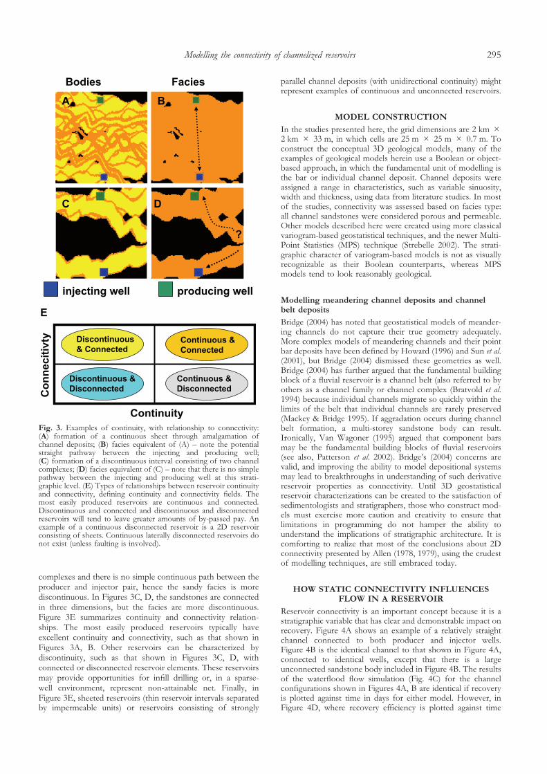
Figure 2C is useful for considering the concept of continuity.Reservoir connectivity and continuity are sometimes usedinterchangeably, yet the terms represent different concepts.Reservoir continuity is best understood by considering direc-tions of continuity. In Figure 2C, it is clear than there is greatercontinuity of sandy facies in the channel-parallel directionthan in the direction perpendicular to channel orientation.Figures 3A, B show a sheet-like reservoir consisting of amalga-mated channel deposits. There is excellent continuity in facies(Fig. 3B) between the injecting and producing well in theexample. In Figures 3C, D, the wells are in different channel

Fig. 2. (A) Static reservoir connectivity may not predict producibilityof the reservoir. Here, a channel is penetrated by a single well. It isunclear whether the entire channel deposit will be depleted by thiswell, even though the reservoir connectivity is 100%. (B) A produc-ing and injecting well are in the same channel geobody (such that theconnectivity is 100%), yet it is unclear whether the entire reservoircan be drained with this well arrangement. (C) Examples of possiblecomplex relationships in a channelized reservoir between injectingand producing wells. Producers with poor communication to inject-ing wells are labelled ‘P’. Dead-end parts of the reservoir, represent-ing channel deposits with no clear communication to producing andinjecting wells are also labelled.

D. K. Larue & J. Hovadik294

complexes and there is no simple continuous path between theproducer and injector pair, hence the sandy facies is morediscontinuous. In Figures 3C, D, the sandstones are connectedin three dimensions, but the facies are more discontinuous.Figure 3E summarizes continuity and connectivity relation-ships. The most easily produced reservoirs typically haveexcellent continuity and connectivity, such as that shown inFigures 3A, B. Other reservoirs can be characterized bydiscontinuity, such as that shown in Figures 3C, D, withconnected or disconnected reservoir elements. These reservoirsmay provide opportunities for infill drilling or, in a sparse-well environment, represent non-attainable net. Finally, inFigure 3E, sheeted reservoirs (thin reservoir intervals separatedby impermeable units) or reservoirs consisting of strongly

parallel channel deposits (with unidirectional continuity) mightrepresent examples of continuous and unconnected reservoirs.

MODEL CONSTRUCTION

In the studies presented here, the grid dimensions are 2 km �2 km � 33 m, in which cells are 25 m � 25 m � 0.7 m. Toconstruct the conceptual 3D geological models, many of theexamples of geological models herein use a Boolean or object-based approach, in which the fundamental unit of modelling isthe bar or individual channel deposit. Channel deposits wereassigned a range in characteristics, such as variable sinuosity,width and thickness, using data from literature studies. In mostof the studies, connectivity was assessed based on facies type:all channel sandstones were considered porous and permeable.Other models described here were created using more classicalvariogram-based geostatistical techniques, and the newer Multi-Point Statistics (MPS) technique (Strebelle 2002). The strati-graphic character of variogram-based models is not as visuallyrecognizable as their Boolean counterparts, whereas MPSmodels tend to look reasonably geological.

Modelling meandering channel deposits and channelbelt deposits

Bridge (2004) has noted that geostatistical models of meander-ing channels do not capture their true geometry adequately.More complex models of meandering channels and their pointbar deposits have been defined by Howard (1996) and Sun et al.(2001), but Bridge (2004) dismissed these geometries as well.Bridge (2004) has further argued that the fundamental buildingblock of a fluvial reservoir is a channel belt (also referred to byothers as a channel family or channel complex (Bratvold et al.1994) because individual channels migrate so quickly within thelimits of the belt that individual channels are rarely preserved(Mackey & Bridge 1995). If aggradation occurs during channelbelt formation, a multi-storey sandstone body can result.Ironically, Van Wagoner (1995) argued that component barsmay be the fundamental building blocks of fluvial reservoirs(see also, Patterson et al. 2002). Bridge’s (2004) concerns arevalid, and improving the ability to model depositional systemsmay lead to breakthroughs in understanding of such derivativereservoir properties as connectivity. Until 3D geostatisticalreservoir characterizations can be created to the satisfaction ofsedimentologists and stratigraphers, those who construct mod-els must exercise more caution and creativity to ensure thatlimitations in programming do not hamper the ability tounderstand the implications of stratigraphic architecture. It iscomforting to realize that most of the conclusions about 2Dconnectivity presented by Allen (1978, 1979), using the crudestof modelling techniques, are still embraced today.

HOW STATIC CONNECTIVITY INFLUENCESFLOW IN A RESERVOIR

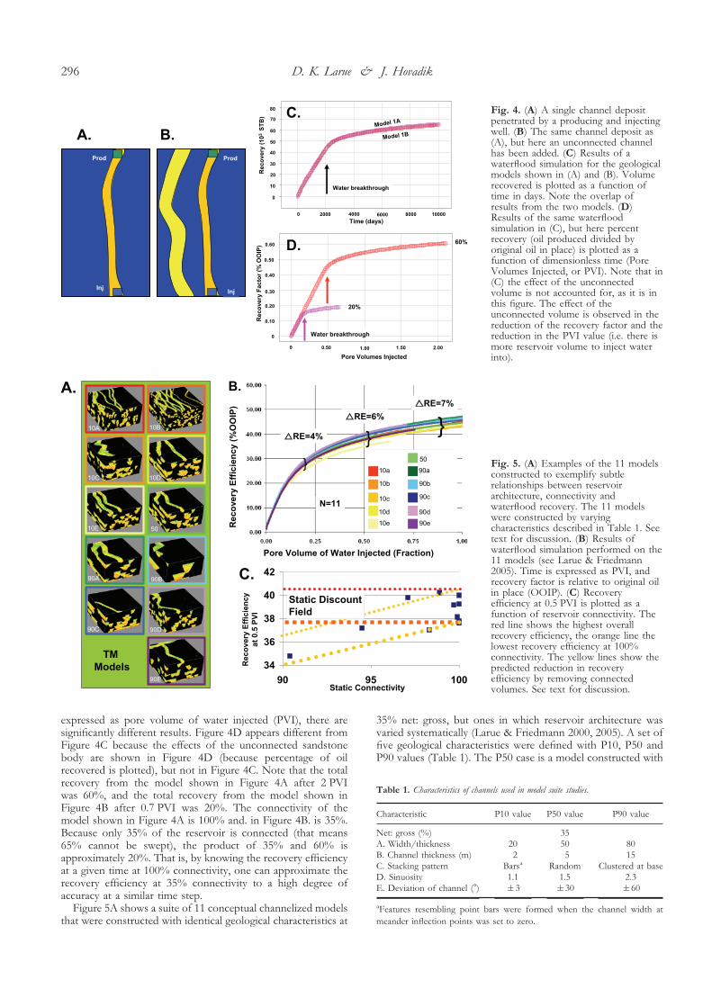
Reservoir connectivity is an important concept because it is astratigraphic variable that has clear and demonstrable impact onrecovery. Figure 4A shows an example of a relatively straightchannel connected to both producer and injector wells.Figure 4B is the identical channel to that shown in Figure 4A,connected to identical wells, except that there is a largeunconnected sandstone body included in Figure 4B. The resultsof the waterflood flow simulation (Fig. 4C) for the channelconfigurations shown in Figures 4A, B are identical if recoveryis plotted against time in days for either model. However, inFigure 4D, where recovery efficiency is plotted against time

Fig. 3. Examples of continuity, with relationship to connectivity:(A) formation of a continuous sheet through amalgamation ofchannel deposits; (B) facies equivalent of (A) – note the potentialstraight pathway between the injecting and producing well;(C) formation of a discontinuous interval consisting of two channelcomplexes; (D) facies equivalent of (C) – note that there is no simplepathway between the injecting and producing well at this strati-graphic level. (E) Types of relationships between reservoir continuityand connectivity, defining continuity and connectivity fields. Themost easily produced reservoirs are continuous and connected.Discontinuous and connected and discontinuous and disconnectedreservoirs will tend to leave greater amounts of by-passed pay. Anexample of a continuous disconnected reservoir is a 2D reservoirconsisting of sheets. Continuous laterally disconnected reservoirs donot exist (unless faulting is involved).

Modelling the connectivity of channelized reservoirs 295

expressed as pore volume of water injected (PVI), there aresignificantly different results. Figure 4D appears different fromFigure 4C because the effects of the unconnected sandstonebody are shown in Figure 4D (because percentage of oilrecovered is plotted), but not in Figure 4C. Note that the totalrecovery from the model shown in Figure 4A after 2 PVIwas 60%, and the total recovery from the model shown inFigure 4B after 0.7 PVI was 20%. The connectivity of themodel shown in Figure 4A is 100% and. in Figure 4B. is 35%.Because only 35% of the reservoir is connected (that means65% cannot be swept), the product of 35% and 60% isapproximately 20%. That is, by knowing the recovery efficiencyat a given time at 100% connectivity, one can approximate therecovery efficiency at 35% connectivity to a high degree ofaccuracy at a similar time step.

Figure 5A shows a suite of 11 conceptual channelized modelsthat were constructed with identical geological characteristics at

35% net: gross, but ones in which reservoir architecture wasvaried systematically (Larue & Friedmann 2000, 2005). A set offive geological characteristics were defined with P10, P50 andP90 values (Table 1). The P50 case is a model constructed with

Fig. 4. (A) A single channel depositpenetrated by a producing and injectingwell. (B) The same channel deposit as(A), but here an unconnected channelhas been added. (C) Results of awaterflood simulation for the geologicalmodels shown in (A) and (B). Volumerecovered is plotted as a function oftime in days. Note the overlap ofresults from the two models. (D)Results of the same waterfloodsimulation in (C), but here percentrecovery (oil produced divided byoriginal oil in place) is plotted as afunction of dimensionless time (PoreVolumes Injected, or PVI). Note that in(C) the effect of the unconnectedvolume is not accounted for, as it is inthis figure. The effect of theunconnected volume is observed in thereduction of the recovery factor and thereduction in the PVI value (i.e. there ismore reservoir volume to inject waterinto).

Fig. 5. (A) Examples of the 11 modelsconstructed to exemplify subtlerelationships between reservoirarchitecture, connectivity andwaterflood recovery. The 11 modelswere constructed by varyingcharacteristics described in Table 1. Seetext for discussion. (B) Results ofwaterflood simulation performed on the11 models (see Larue & Friedmann2005). Time is expressed as PVI, andrecovery factor is relative to original oilin place (OOIP). (C) Recoveryefficiency at 0.5 PVI is plotted as afunction of reservoir connectivity. Thered line shows the highest overallrecovery efficiency, the orange line thelowest recovery efficiency at 100%connectivity. The yellow lines show thepredicted reduction in recoveryefficiency by removing connectedvolumes. See text for discussion.

Table 1. Characteristics of channels used in model suite studies.

Characteristic P10 value P50 value P90 value

Net: gross (%) 35A. Width/thickness 20 50 80B. Channel thickness (m) 2 5 15C. Stacking pattern Barsa Random Clustered at baseD. Sinuosity 1.1 1.5 2.3E. Deviation of channel (�) �3 �30 �60

aFeatures resembling point bars were formed when the channel width atmeander inflection points was set to zero.

D. K. Larue & J. Hovadik296

only P50 values. Then ten additional models were constructedusing P50 values and one P10 or P90 value. The model namerefers to which parameter was varied. A waterflood pore-voidage replacement simulation was performed on each modelusing a 110-acre well spacing. Results are shown in Figure 5Band the range in recovery efficiency at a given PVI is on theorder of 5–7%. Given that the models are identical in allrespects except reservoir architecture, what caused this vari-ation in flow performance? Was it due to changes in reservoirarchitecture? Was it simply some random effect? In Figure 5C,the static connectivity of the models is plotted against therecovery after 0.5 PVI. There seems to be a weak linear trend,such that recovery efficiency appears to be related to connec-tivity. The red line in the figure shows the highest recoveryefficiency of any model (approximately 40.5%) and the orangeline shows the lowest recovery efficiency for any 100% con-nected model. The 2% spread in recovery efficiencybetween the orange and red lines is probably due to slightdifferences in permeability heterogeneity between the models.The yellow lines shows how the recovery efficiency shoulddegrade if reducing connectivity effectively removes ‘sweepable’volumes from the reservoir. The slope of the upper yellow linepredicts that if the recovery efficiency is 40.5% at 100%connectivity, then at 90% connectivity, the recovery efficiencyshould be about 36.5%. For the lower yellow line, the recoveryefficiency should be about 34% at 90% connectivity. Note thatthe points, representing different flow simulation results, fallmostly between these lines. If a point falls above the banddefined by the yellow lines, this means that sweep efficiency isenhanced with reduction of sweepable reservoir volume. If thepoints fall within the band, it means that reduction in connec-tivity effectively predicts reduction in recovery efficiency.Finally, if the points fall below the band, it means that otherfactors beyond static connectivity reduction may be reducingrecovery efficiency.

Based on these two examples, a clear relationship betweenreservoir connectivity and flow performance can be expected.

CONNECTIVITY AS A FUNCTION OF NET: GROSS

Two dimensions: the ‘S-curve’

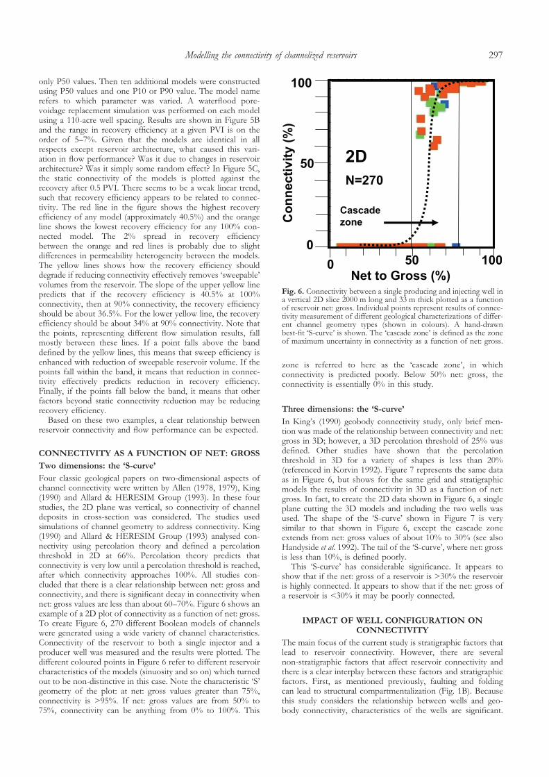
Four classic geological papers on two-dimensional aspects ofchannel connectivity were written by Allen (1978, 1979), King(1990) and Allard & HERESIM Group (1993). In these fourstudies, the 2D plane was vertical, so connectivity of channeldeposits in cross-section was considered. The studies usedsimulations of channel geometry to address connectivity. King(1990) and Allard & HERESIM Group (1993) analysed con-nectivity using percolation theory and defined a percolationthreshold in 2D at 66%. Percolation theory predicts thatconnectivity is very low until a percolation threshold is reached,after which connectivity approaches 100%. All studies con-cluded that there is a clear relationship between net: gross andconnectivity, and there is significant decay in connectivity whennet: gross values are less than about 60–70%. Figure 6 shows anexample of a 2D plot of connectivity as a function of net: gross.To create Figure 6, 270 different Boolean models of channelswere generated using a wide variety of channel characteristics.Connectivity of the reservoir to both a single injector and aproducer well was measured and the results were plotted. Thedifferent coloured points in Figure 6 refer to different reservoircharacteristics of the models (sinuosity and so on) which turnedout to be non-distinctive in this case. Note the characteristic ‘S’geometry of the plot: at net: gross values greater than 75%,connectivity is >95%. If net: gross values are from 50% to75%, connectivity can be anything from 0% to 100%. This

zone is referred to here as the ‘cascade zone’, in whichconnectivity is predicted poorly. Below 50% net: gross, theconnectivity is essentially 0% in this study.

Three dimensions: the ‘S-curve’

In King’s (1990) geobody connectivity study, only brief men-tion was made of the relationship between connectivity and net:gross in 3D; however, a 3D percolation threshold of 25% wasdefined. Other studies have shown that the percolationthreshold in 3D for a variety of shapes is less than 20%(referenced in Korvin 1992). Figure 7 represents the same dataas in Figure 6, but shows for the same grid and stratigraphicmodels the results of connectivity in 3D as a function of net:gross. In fact, to create the 2D data shown in Figure 6, a singleplane cutting the 3D models and including the two wells wasused. The shape of the ‘S-curve’ shown in Figure 7 is verysimilar to that shown in Figure 6, except the cascade zoneextends from net: gross values of about 10% to 30% (see alsoHandyside et al. 1992). The tail of the ‘S-curve’, where net: grossis less than 10%, is defined poorly.

This ‘S-curve’ has considerable significance. It appears toshow that if the net: gross of a reservoir is >30% the reservoiris highly connected. It appears to show that if the net: gross ofa reservoir is <30% it may be poorly connected.

IMPACT OF WELL CONFIGURATION ONCONNECTIVITY

The main focus of the current study is stratigraphic factors thatlead to reservoir connectivity. However, there are severalnon-stratigraphic factors that affect reservoir connectivity andthere is a clear interplay between these factors and stratigraphicfactors. First, as mentioned previously, faulting and foldingcan lead to structural compartmentalization (Fig. 1B). Becausethis study considers the relationship between wells and geo-body connectivity, characteristics of the wells are significant.

Fig. 6. Connectivity between a single producing and injecting well ina vertical 2D slice 2000 m long and 33 m thick plotted as a functionof reservoir net: gross. Individual points represent results of connec-tivity measurement of different geological characterizations of differ-ent channel geometry types (shown in colours). A hand-drawnbest-fit ‘S-curve’ is shown. The ‘cascade zone’ is defined as the zoneof maximum uncertainty in connectivity as a function of net: gross.

Modelling the connectivity of channelized reservoirs 297

Figure 8A compares geobody connectivity, single injector orproducer connectivity (that is, only two wells within the 2 km2

area) and injector to producer connectivity for 200 conceptualreservoir characterizations. Note that the most rigorous ofconnectivity definitions – injector to producer connectivity (forexample, Fig. 1F) – results in a slight shifting of the ‘S-curve’ tothe right, toward worse connectivity. In Figure 8B, the influ-ence of well count on connectivity is shown (see also Budding& Paardekam 1992). Note that for a 12-fold increase in welldensity, the cascade zone shifts to the left by about 10% in net:gross. To examine this effect more quantitatively, a suite of 200geological models was built at 20%, 30% and 40% net: gross,and analysed for the two well groups (Fig. 8C). At 20% net:gross, the connectivity dropped 41%, whereas at 30% theconnectivity dropped 10%, while at 40% the connectivitydropped only 3%. Differences in connectivity are largelyassociated with wells with zero connectivity or those that donot intersect the reservoir. In Figure 8D, the effects ofcompletions are considered (for example, Fig. 1G). Onlyportions of wellbores are completed to minimize costs, or toprevent water influx. In one group of models, the entire 33 mwellbore is completed, whereas, in the second, only the top 3 mof the model is completed. In all cases. and as summarized inthe embedded table, the average connectivity drops significantly(mostly due to 0% connectivity values). This large drop inconnectivity is, in part, due to how the completions weredefined: the top 3 m of the model was completed whether ornot sandbodies were present, so these results represent anunrealistically pessimistic case. The impact of completions onconnectivity is minimized with a higher well count (Fig. 8E).Orientation of the producer–injector pair, whether vertical orhorizontal, and parallel or perpendicular to the channel direc-tion, can also affect connectivity (Figs 8F, G) and is probablybest considered on a case-by-case basis.

INCREASED VARIANCE OF GEOLOGICALCHARACTERISTICS: STRATIGRAPHIC FACTORS

The eleven geological models shown in Figure 5 were createdby changing geological characteristics one by one at a fixed net:gross value of 35% (Table 1). Additional models were built

using parameters described in Table 1 at net: gross valuesbetween 0% and 100%. Three hundred realizations werecreated for each model type. Producer–injector reservoir con-nectivity for a single well pair (again, two wells in a 2 km2 area)was calculated for each model realization and results are plottedas a function of net: gross in Figure 9. The resulting ‘S-curve’shows much greater variability than that shown in Figure 7.Figure 9L summarizes each model type (Figs 9A–K) and showsreservoir connectivity for net: gross values greater than 35%: inthis way, stratigraphic factors that lead to worse connectivitycan be analysed quickly. Geological factors that promotegreater variance in connectivity are straighter (Fig. 9D), moreparallel (Fig. 9E), wider (Fig. 9G) and thicker (Fig. 9H)channels, relative to the average channel values shown inTable 1. Geological factors that promote less variance inconnectivity relative to the average values are thinner (Fig. 9B),narrower (Fig. 9A), more sinuous (Fig. 9J), non-parallel(Fig. 9K) channel deposits. In addition, channel depositscomposed of bars also tend to show better connectivity thanthe average values (Fig. 9C). Clearly, there is a relationshipbetween reservoir architecture and reservoir connectivity. Theorigins of this relationship and, more generally, factors thattend to increase or decrease connectivity, will be the subject ofcontinued investigation in this study.

FACTORS THAT IMPROVE CONNECTIVITY:SHIFTING THE ‘S-CURVE’ TO THE LEFT

Although the shapes of the ‘S-curves’ shown in Figures 7 and 9would appear to represent relatively optimistic reservoir con-ditions, they can be made even more optimistic under certainstratigraphic conditions. To make the ‘S-curve’ more optimistic,higher connectivities would be observed in lower net: grossrocks. How can this occur? In a mud-rich setting, why wouldconnectivity be high?

Overbank sandy facies

Clearly, the occurrence of overbank sandy facies, such as sandylevees, crevasse-splay or sheet-flood deposits could serve toconnect unconnected channel deposits at any net: gross(Fig. 10A). Sandy overbank facies may be characterized bydifferent permeability distributions and by variable and uncer-tain continuity. However, clearly they could serve as importantlateral conduits in channelized successions.

Width to thickness ratios of channel deposits

If the width to thickness ratio of channel deposits wasextremely high, or if sheet-like deposits were present, thenconnectivity could be achieved at very low net: gross values(Fig. 10B). Channel complexes represent the lateral and verticalamalgamation of smaller channel bodies, such that the channelcomplex has a larger width/thickness ratio (Fig. 10C). Thisenhanced width/thickness ratio should increase connectivity atlow net: gross values. For the models described in Figure 9,better connectivity was shown to be associated with narrowerchannel deposits than wider channel deposits (compare Figs 9Aand G). This apparent refutation of the proposed relationshipbetween channel width and enhanced connectivity is a functionof the grid volume and the modelling process. At low net: grossvalues, it is more likely that edges of channels are inserted intothe grid (that is, the channel centre is located outside of the gridvolume) and connectivity is limited by channel edges. However,this effect is really a function of the size of the object to thevolume of the study area (a volume effect) and is described ingreater detail later.

Fig. 7. Same data as Figure 6, but here the connectivity is measuredin 3D in a volume 2000 m � 2000 m � 33 m. Note the shifting ofthe ‘S-curve’ and the cascade zone to the left.

D. K. Larue & J. Hovadik298

Fig. 8. (A) Three-dimensional connectivity for 200 conceptual Boolean models. Four types of connectivity were measured: geobody connectivity,connectivity to the producer well, connectivity to the injector well, and connectivity from the injector to the producer well. Note that theconnectivity from injector to producer is slightly more pessimistic than the other types of connectivity (that is, the ‘S-curve’ is shifted to the right),which largely overlap. (B) Influence of well density on connectivity. Here, 3D injector to producer connectivity is compared for one well pairversus 12 well pairs in the 4 km2 area. (C) Six hundred additional geological realizations were created at net: gross values of 20%, 30% and 40%,and connectivities were compared for one injector–producer pair and 12 pairs (patterns). Average results are summarized in the table, and showthat the importance of well density for reservoir connectivity diminishes at higher net: gross values. Note that the most significance impact onaverage connectivity for the 30% and 40% net: gross examples are wells that do not intersect reservoir (i.e. wells in which connectivity is 0%).(D) The importance of the completion interval is shown for the same dataset as in (C). The connectivity of two wells with open-hole completionsis compared with two wells with 10 ft (3 m) completions. The effect of the limited completions was made worse because no requirement for sandpresence was made (although no requirement for sand presence was made for the open hole either). Average results shown in table. (E) Theimportance of the completion interval is shown for the same dataset as in (C). The connectivity of 12 well pairs (or patterns) with open-holecompletions is compared with 12 well pairs with 10 ft completions. The effect of the limited completions was made worse because no requirementfor sand presence was made (although no requirement for sand presence was made for the open hole either). Average results shown in table.(F) Effect of well orientation with respect to stratigraphic trend is shown for the same model dataset. Connectivity of vertical well pairs incross-channel and down-channel directions is compared. Connectivity of horizontal well pairs oriented cross channel and down channel iscompared. (G) Using the dataset of (C), well orientation connectivity effects are studied at 20%, 30% and 40% net: gross.

Modelling the connectivity of channelized reservoirs 299

Fig

.9.

Res

ults

ofth

ousa

nds

ofge

olog

ical

sim

ulat

ions

ofch

anne

lsan

dre

serv

oir

elem

ents

ofdi

ffer

ent

geom

etrie

s.E

ach

poin

tre

pres

ents

mea

sure

men

tof

inje

ctor

topr

oduc

erco

nnec

tivity

ona

sepa

rate

geol

ogic

alch

arac

teriz

atio

n.E

ach

geol

ogic

alm

odel

is20

00m

�20

00m

�33

m.B

asic

geol

ogic

alpa

ram

eter

sfo

rcr

eatin

gth

em

odel

sar

esh

own

inT

able

1,on

lyne

t:gr

oss

valu

esar

eal

low

edto

vary

betw

een

0%an

d10

0%.T

hear

row

atth

ebo

ttom

ofea

chgr

aph

show

sth

ehi

ghes

tne

t:gr

oss

with

0%co

nnec

tivity

and

rang

esfr

omab

out

20–4

0%ne

t:gr

oss.

The

red

line

show

sth

e35

%de

mar

catio

npo

int

used

inFi

gure

9L.(

A)

Nar

row

chan

nels

;cha

nnel

wid

th/t

hick

ness

ratio

is20

.All

othe

rva

lues

are

show

nas

P50

valu

esin

Tab

le1.

(B)

Thi

nch

anne

ls,2

mth

ick.

(C)

Cha

nnel

bars

repr

esen

tth

edo

min

ant

fluvi

alel

emen

t.(D

)St

raig

htch

anne

ls.(

E)

Para

llelc

hann

els.

(F)

P50

case

inT

able

1.(G

)W

ide

chan

nels

,in

whi

chw

idth

/thi

ckne

ssis

80.(

H)

Thi

ckch

anne

ls,1

5m

thic

k.(I

)St

acke

dch

anne

ls,i

nw

hich

mor

ech

anne

lsoc

cur

near

the

base

ofth

em

odel

.(J)

Sinu

ous

chan

nels

,with

sinu

osity

ofab

out

2.3.

(K)

Non

-par

alle

lcha

nnel

s,sh

owin

gla

rge

devi

atio

nin

orie

ntat

ion.

(L)

Sum

mar

ypl

ot:c

onne

ctiv

ityfo

rm

odel

sw

ithne

t:gr

oss

grea

ter

than

35%

plot

ted

agai

nst

run

num

ber.

See

text

for

disc

ussi

on.

D. K. Larue & J. Hovadik300

By making the channel deposits even wider, relative tothickness, connectivity will increase at a given net: gross. In thelimiting case of sheet deposits that extend over the entirereservoir area, 100% connectivity could be achieved even if thenet: gross value was exceedingly low.

Variable floodplain aggradation rates

If the rate of floodplain aggradation was punctuated, such thatperiods of rapid aggradation alternated with periods of slowaggradation, channelized sheets could be formed amidst discon-nected channel deposits (Fig. 10D). That is, during periodsof rapid floodplain aggradation, abundant muddy overbankdeposits would be preserved. During periods of slow floodplainaggradation, mostly erosive channel deposits would be pre-served, and abundant lateral amalgamation would occur, form-ing channelized sheets. The formation of these channelizedsheets is compatible with interpretations based on sequencestratigraphic concepts (Shanley & McCabe 1994). Of course,net: gross is actually changing in the vertical sense, such thatperiods of low aggradation rates are associated with preserva-tion of higher net: gross intervals. However, vertical variationsin net: gross are commonly missed in stratigraphic studies thatdo not emphasize sequence stratigraphic concepts.

FACTORS THAT REDUCE CONNECTIVITY:SHIFTING THE ‘S-CURVE’ TO THE RIGHT

How can the ‘S-curve’ in Figure 7 be made to be lessoptimistic? How can lower connectivities occur at higher net:gross ratios? If reservoirs were two dimensional, then theirconnectivity would be greatly reduced, but how can a reservoirbe 2D? In outcrops of cliff faces or in cross-section (such asthose shown in Fig. 1), channel deposits that do not intersect in2D may intersect in 3D. Quasi-two-dimensional reservoirs doexist in nature and there are essentially two types.

Two-dimensional reservoirs with parallel channeldeposits

If channels are relatively straight and parallel, and therefore donot intersect in a given stratigraphic layer, the reservoir will

behave as a quasi-2D model (obviously, what happens aboveand below the given time slice can affect the true twodimensionality of the model). Figure 11A shows a conceptualexample of parallel channels in a waterflood situation. Becauseof parallelism of the channels, there is relatively poor connec-tivity at least in the plane of this figure. Results of modellingchannels that range in character from perfectly straight andparallel to parallel and sinuous are shown in Figure 12A.Perfectly parallel straight channel deposits in three dimensionsshould behave as quasi-2D objects and this is observed inFigure 12A. As the straight parallel channel deposits becomeprogressively more sinuous, the connectivity shifts from 2D to3D. In Figure 12B, results of modelling channel deposits thatrange in character from perfectly straight and parallel to straightand deviated in orientation are shown. In a similar way to theexample of sinuous channel deposits, as the straight andparallel channel deposits become progressively more varied inorientation, the connectivity shifts from 2D to 3D.

The poorer connectivity noted previously of models shownin Figure 9E relative to Figure 9K is apparently associated witha weak 2D component to the models.

Two-dimensional sheeted reservoirs

Quasi-2D reservoirs may result from laterally continuousheterogeneities (Fig. 11B). If a reservoir is vertically stratifiedinto separate reservoir compartments, and the stratificationthickness is approximately the same as the channel thickness,then the reservoir will behave as a quasi-2D reservoir. Mud-stones deposited on top of flooding surfaces or abandonmentsurfaces in fluvial strata, or associated with condensed intervalscould cause vertical stratification. Vertical reservoir stratifica-tion could also be produced by continuous muddy debris flowunits, continuous hemipelagic intervals, or continuous muddyturbidite deposits. Essentially any impermeable mudstone unit

Fig. 10. Stratigraphic factors that cause shifting of the ‘S-curve’ tothe left, toward better connectivity. (A) Channel width can beaugmented by lateral sandy facies such as crevasse splays and levees.(B) Channels with high width/thickness ratio will tend to shift the‘S-curve’ to the left, although a volume support effect can complicateinterpretations (see text for discussion). (C) Genetic clusters ofchannels, also known as channel belts, channel families or channelcomplexes result in reservoir units with greater width/thicknessratio. (D) Due to periods of minimal floodplain aggradation, lateralchannel shifting results in lateral channel amalgamation and forma-tion of complexes that have greater width/thickness ratios.

Fig. 11. Stratigraphic factors that cause shifting of the ‘S-curve’ tothe right, toward worse connectivity. (A) Strongly parallel channelpaths tend not to intersect in map-view, causing 2D connectivity inthat plane. Note the complex relationships between injector andproducer wells. (B) Continuous mudstone units between thin chan-nelized units stratify the reservoir such that it behaves as a series of2D volumes. (C) Local heterogeneous impermeable units compart-mentalize the reservoir. In the top (1), a mudstone drape coats thebase of the channel, causing compartmentalization between other-wise amalgamated channels. In the centre (2), continuous horizontalmudstone beds within a channel can also effectively compartmental-ize the reservoir. Finally, near the bottom (3), inclined heterolithicunits can cause reservoir compartmentalization. (D) Compensationalstacking of channels could in theory result in a poorly connectedsand-rich reservoir. See text for discussion.

Modelling the connectivity of channelized reservoirs 301

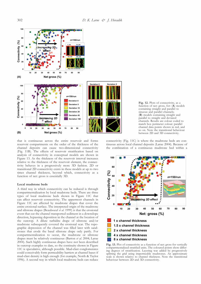
that is continuous across the entire reservoir and formsreservoir compartments on the order of the thickness of thechannel deposits can cause two-dimensional connectivity(Fig. 11B). The effects of reservoir stratification based onanalysis of connectivity in conceptual models are shown inFigure 13. As the thickness of the reservoir interval increasesrelative to the thickness of the reservoir element, the connec-tivity behaves in a progressively more 3D fashion. 2D ortransitional 2D connectivity exists in these models at up to twotimes channel thickness, beyond which, connectivity as afunction of net: gross is essentially 3D.

Local mudstone beds

A third way in which connectivity can be reduced is throughcompartmentalization by local mudstone beds. There are threetypes of local mudstone beds shown in Figure 11C thatcan affect reservoir connectivity. The uppermost channels inFigure 11C are affected by mudstone drapes that cover theentire erosional surface. The interpreted origin of the mudstoneand siltstone drapes (Beauboeuf et al. 1999) is that the erosionalevent that cut the channel transported sediment in a downslopedirection, bypassing deposition in the channel at the location ofthe outcrop. A dilute turbidite drape of siltstone and/ormudstone subsequently covered the erosional scar. The topo-graphic depression of the channel was filled later with sand-stones that erode the basal siltstone drape only partly. Forcompartmentalization to occur, the mudstone or siltstonedrapes must be relatively continuous (Barton et al. 2004; Larue2004). Such highly continuous drapes have not been describedin outcrop examples to date, so the continuity shown in Figure11C is speculative, although possible. Mud-clast conglomeratescould conceivably form permeability barriers at channel bases ifmud-clast density is high enough (for example, North & Taylor1996). A second way in which local mudstone beds can reduce

connectivity (Fig. 11C) is where the mudstone beds are con-tinuous across local channel deposits (Larue 2004). Because ofthe combination of a continuous mudstone bed within a

Fig. 12. Plots of connectivity, as afunction of net: gross, for: (A) modelscontaining straight and parallel tosinuous and parallel channels;(B) models containing straight andparallel to straight and deviatedchannels. Results are colour coded tomatch box perimeter colour: parallelchannel data points shown in red, andso on. Note the transitional behaviourbetween 2D and 3D connectivity.

Fig. 13. Plot of connectivity as a function of net: gross for verticallycompartmentalized stratified units. The coloured points show differ-ing degrees of stratification. Layering was added by progressivelysplitting the grid using impermeable mudstones. An approximatescale is shown relative to channel thickness. Note the transitionalbehaviour between 2D and 3D connectivity.

D. K. Larue & J. Hovadik302

channelized body, a disconnected sandstone body can result.The third way in which local mudstone beds can reduceconnectivity (Fig. 11C, bottom) is where mud-draped clino-forms compartmentalize the reservoir. Mud-draped clinoformswithin a channel can be associated with lateral accretionsurfaces and inclined heterolithic stratification (Thomas et al.1987).

Compensational stacking of channels

There are several ways in which channel deposits can bemodelled. Channel deposits can be modelled such that there isequal probability that a channel can occur anywhere in thesimulation volume. Channel deposits can also be modelled suchthere are vertical and/or lateral trends, and channels are morelikely to occur in some places than others. Channel clusteringcan also be accomplished by modelling channel families, whichare groups of spatially related channel deposits (Bratvold et al.1994; Tyler et al. 1995). More generally, attraction or repulsionproperties may be assigned such that channels tend to clusteror avoid one another spatially. All of these approaches arestochastic representations of natural processes. In general,when a given channel is simulated using standard geostatisticaltechniques, it does not know about channels that have beendeposited previously in the same area.

In the case of compensational stacking, the position of anunderlying deposit strongly impacts the position of subsequentdeposits (for examples, Mutti & Sonnino 1981; King & Browne2001). For example, if a submarine channel is filled withsandstone, and the adjacent mudstones compact around thissandstone, then the channel deposit will form a topographicridge that subsequent channel deposits could avoid (Fig. 11D).Such compensational stacking could lead to relatively high net:gross reservoirs (60%?) with poor connectivity. However, it isimportant to stress that most compensational stacking patternshave been defined for depositional lobes (Mutti & Sonnino1981), channel complexes and larger-scale submarine fanfeatures (King & Browne 2001). What is not known is how finea scale such compensational stacking patterns can be, how tomodel them or what the connectivity might be. A modellingprogram for submarine channel deposition that addressedcompensational stacking patterns was created by Jones & Larue(1997).

FACTORS THAT AFFECT CONNECTIVITY:SHIFTING THE ‘S-CURVE’ IN EITHER

DIRECTION

Volume support

Volume support addresses the issue of whether there issufficient reservoir volume for connectivity to be achieved(King 1990). Referring again to Figure 9, models with morevaried connectivity are those in which the ratio of the volumeof the channel object to the volume of the containing box ishighest (Figs 9G, H). Conversely, models with channel depositsof lesser volume relative to the volume of the container haveless variance in connectivity (Figs 9A, B, C).

An example of the importance of support volume is shownin Figure 14. In this example, five identical channel modelswere built, where channel width/thickness and net: gross werethe only variables. As the channel deposits become biggerrelative to the volume of the gridded volume, the resultingconnectivity becomes more variable. King (1990) showed thatin 2D, volume support effects tend to flatten the ‘S-curve’ suchthat above the percolation threshold, connectivity is reduced,

while below the percolation threshold, connectivity tends to beincreased.

EXAMPLES OF OTHER STRATIGRAPHICFACTORS THAT MAY AFFECT RESERVOIR

CONNECTIVITY

In the search for other factors that may affect reservoirconnectivity, several other stratigraphic situations and processeswere studied.

Connectivity of cell-based geological models

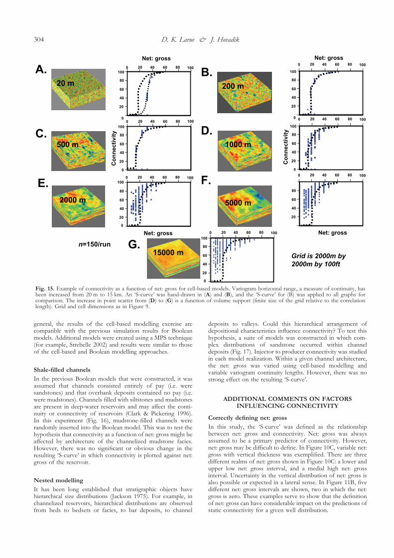
Boolean modelling techniques were used in this study tocharacterize channel deposits in 3D. Another modelling tech-nique commonly employed in the petroleum industry uses acell-based or pixel-based approach (Deutsch & Journel 1997).Cell-based models rely on variograms to distribute rock prop-erties throughout the model. Key characteristics of variogramsare their type and range. Common types of variograms arespherical, Gaussian and exponential, characterized by differencerates of change in variance with distance. Variogram range is ameasure of continuity in 3D. In this experiment, horizontalvariogram range was varied for exponential variograms. Con-nectivity is plotted as a function of net: gross in Figures 15A–G.For shorter ranges relative to the volume of the grid, the typical‘S-curve’ is produced from the simulation results, in whichconnectivity rapidly diminishes at net: gross values less thanabout 35% (Figs 15 A–C). In Figures 15D–G, there is progres-sively greater scatter in the ‘S-curve’ for a given net: gross. Thisincrease in scatter is due to two effects – increasing width/thickness of the facies continuity and volume support effects.Increasing the continuity range has a similar effect to increasingthe width/thickness of the facies bodies. This allows higherconnectivity at lower net: gross values. However, as thecontinuity range is increased, there are also increasing examplesof lower connectivity at higher net: gross values. This volumesupport effect is due to the fact that the volume of the box islimited relative to the size of the modelled continuity. In

Fig. 14. (A) Example of volume support issue. A series of identicalmodels were constructed at a range of net: gross values, but thewidth of the channel was increased in each model. (B) Plot ofconnectivity as a function of model run, for model runs in which thenet: gross was greater than 35%. With increasing model run, theconnectivity becomes progressively worse, which is a function ofvolume support. (C) Examples of the models used to study volumesupport.

Modelling the connectivity of channelized reservoirs 303

general, the results of the cell-based modelling exercise arecompatible with the previous simulation results for Booleanmodels. Additional models were created using a MPS technique(for example, Strebelle 2002) and results were similar to thoseof the cell-based and Boolean modelling approaches.

Shale-filled channels

In the previous Boolean models that were constructed, it wasassumed that channels consisted entirely of pay (i.e. weresandstones) and that overbank deposits contained no pay (i.e.were mudstones). Channels filled with siltstones and mudstonesare present in deep-water reservoirs and may affect the conti-nuity or connectivity of reservoirs (Clark & Pickering 1996).In this experiment (Fig. 16), mudstone-filled channels wererandomly inserted into the Boolean model. This was to test thehypothesis that connectivity as a function of net: gross might beaffected by architecture of the channelized mudstone facies.However, there was no significant or obvious change in theresulting ‘S-curve’ in which connectivity is plotted against net:gross of the reservoir.

Nested modelling

It has been long established that stratigraphic objects havehierarchical size distributions (Jackson 1975). For example, inchannelized reservoirs, hierarchical distributions are observedfrom beds to bedsets or facies, to bar deposits, to channel

deposits to valleys. Could this hierarchical arrangement ofdepositional characteristics influence connectivity? To test thishypothesis, a suite of models was constructed in which com-plex distributions of sandstone occurred within channeldeposits (Fig. 17). Injector to producer connectivity was studiedin each model realization. Within a given channel architecture,the net: gross was varied using cell-based modelling andvariable variogram continuity lengths. However, there was nostrong effect on the resulting ‘S-curve’.

ADDITIONAL COMMENTS ON FACTORSINFLUENCING CONNECTIVITY

Correctly defining net: gross

In this study, the ‘S-curve’ was defined as the relationshipbetween net: gross and connectivity. Net: gross was alwaysassumed to be a primary predictor of connectivity. However,net: gross may be difficult to define. In Figure 10C, variable net:gross with vertical thickness was exemplified. There are threedifferent realms of net: gross shown in Figure 10C: a lower andupper low net: gross interval, and a medial high net: grossinterval. Uncertainty in the vertical distribution of net: gross isalso possible or expected in a lateral sense. In Figure 11B, fivedifferent net: gross intervals are shown, two in which the net:gross is zero. These examples serve to show that the definitionof net: gross can have considerable impact on the predictions ofstatic connectivity for a given well distribution.

Fig. 15. Example of connectivity as a function of net: gross for cell-based models. Variogram horizontal range, a measure of continuity, hasbeen increased from 20 m to 15 km. An ‘S-curve’ was hand-drawn in (A) and (B), and the ‘S-curve’ for (B) was applied to all graphs forcomparison. The increase in point scatter from (D) to (G) is a function of volume support (finite size of the grid relative to the correlationlength). Grid and cell dimensions as in Figure 9.

D. K. Larue & J. Hovadik304

Interplay of fault compartmentalization and reservoirconnectivity

Although faulting is clearly one of the major causes for aerialcompartmentalization of reservoirs (Fig. 1B), the present studyhas concentrated on stratigraphic origins of reservoir compart-ments. There is an interesting potential interplay between faultcompartmentalization and reservoir connectivity. Previous

studies have noted that reservoirs tend to become morestructurally compartmentalized with production history due tothe increase in the amount of data with time, primarilywell-based and production (for example, Bentley & Barry 1991;Demyttenaere et al. 1993). As it becomes apparent that areservoir is more structurally compartmentalized than pre-viously believed, this reduction in support volume should leadto reassessment of the potential for additional stratigraphiccompartmentalization as well. That is, it was shown previouslythat reducing the support volume of a reservoir typicallyimpacts the static connectivity of the reservoir negatively.

Connectivity as a function of distance: dynamicinterpretations of connectivity

As has been demonstrated herein, calculation of reservoirconnectivity in 3D models tends to give optimistic results. Fornet: gross values greater than about 30% – and barring othercomplications or situations described above – connectivitytends to be >90% and therefore does not impact recoveryefficiency significantly. As a result, there have been attempts toredefine connectivity such that it is more sensitive to geologicalsituations. One such attempt is to define connectivity as afunction of distance (for example, Hird & Dubrule 1998).Connectivity as a function of distance addresses the fact thatinfinite time is not available to drain tortuously connectedreservoirs, such as those portrayed in Figures 2A–C. Bydefining some characteristic length away from the well, a moreconservative definition of connectivity can be made. Connec-tivity as a function of distance represents an important directionin connectivity studies.

CONCLUSIONS

A fundamental ‘S-curve’ relationship between net: gross andreservoir connectivity has been described, as well as means inwhich the ‘S-curve’ can be translated to enhance or degradereservoir connectivity as a function of net: gross. Althoughresults are based on geostatistical models, general conclusionsare believed applicable to reservoir characterization studies.Any use of conclusions presented herein must be made in

Fig. 16. Connectivity degradation byshale-filled channels. Differentquantities of shale-filled channels wereadded to model simulations to test theeffect of connectivity degradation byshale-filled channels. See text fordiscussion. (A) Plot of connectivity as afunction of net: gross for models withdifferent amounts of shale-filledchannels. (B) Example of obliqueview of sand-filled and shale-filledchannels. Shale-filled channelshave been removed for the model.(C) Cross-section view of sand-filledand shale-filled (black) channels..

Fig. 17. The effect of nested architecture on reservoir connectivity.Two examples of channel architecture are shown with variablechannel fill of sandstone and shale. In these models, mudstone canoccur both as overbank deposits and as shales deposited within thechannels. The set of models was characterized by channel width/thickness ratios of (A) 25 and (B) of 100, both with variablequantities of shale infilling the channel deposits. Range of thevariogram for modelling shale was 5000 m to ensure that the layeringwas continuous. As the amount of shale increased within the channelfill, the connectivity tended to follow the direction shown by thepurple arrow, toward better connectivity at lower net: gross values.This is probably because the ordering of the channels enhancesconnectivity.

Modelling the connectivity of channelized reservoirs 305

light of non-stationarity issues, sequence stratigraphic originsand non-random stacking patterns, as described in the textpreviously.

Table 2 discusses some of the factors found to enhance ordegrade reservoir connectivity and how to recognize theseeffects in a given field. For example, large reservoir elementwidth/thickness ratios clearly enhance connectivity in absenceof volume support effects (Figs 10A, B). Reservoir elementwidth/thickness can be determined using well-log correlationstudies, charts of width/thickness, statistical techniques orbased on sequence stratigraphic studies. Variable aggradationrates of a floodplain (Fig. 10D) can result in enhanced ordegraded reservoir connectivity and can be established throughsequence stratigraphic studies. Two-dimensional effects, suchas parallel channel deposits and thin sheets of reservoir, canresult in poorly connected reservoirs. Recognition of parallelchannel deposits (Fig. 2C) can be made through reservoirarchitecture studies (Barton et al. 2004), seismic analysis andpossibly through production studies. Recognition of sheetedreservoir intervals can be made through well-log correlationstudies tied to core studies. A two-dimensional sheeted reser-voir is defined as one whose reservoir element thickness (forexample channel thickness) is approximately the same as thereservoir interval thickness (Fig. 11B). Certain types of continu-ous mudstone beds, including basal mudstone beds and con-tinuous mudstones within channel fills, can compartmentalizereservoirs with respect to wells (Fig. 11C). Recognition ofcontinuous mudstone beds can be made through core andwell-log study. Key features are thick mudstone beds alongchannel bottoms, and thick mudstone or debris flow unitswithin channel deposits. Compensational stacking can occurwhen channels are deposited while avoiding the position ofunderlying channels (Fig. 11D). Recognition of compensationalstacking patterns has only been made in depositional lobes andchannel complexes, and not at the channel deposit scale,

though this could occur. Finally, the size of the gross containercan affect reservoir connectivity (Figs 14A–C). If the size of thereservoir element is a sizeable fraction of the length of thecontainer, then volume support effects may occur. In thesestudies, the container was 2000 m long and volume supporteffects were noted in Boolean objects with widths greater than200 m and in cell-based models with ranges greater than1000 m.

It is those factors that shift the ‘S-curve’ to the right that arethe most important for addressing potential downside scenariosfor sparse-well development studies, in which only a few wellsare used to drain the reservoir, and for considerations of laterinfill drilling. The potential impact of these factors can beaddressed using careful geological analysis.

The authors thank the Chevron Corporation for allowing publicationof this paper. The Chevron Corporation is also acknowledged andthanked for supporting research on this topic for a number of years.Discussions with Ron Behrens, Connie Terricola, Andrew Latham,June Gidman, Frank Harris, Tim McHargue, John Toldi et al. werevery important in the evolution of thoughts in this paper. Finally, thefirst author would like to thank Danny Horowitz, formerly ofSwanson Consulting, who helped him appreciate how connectivitycould be modelled and analysed.

REFERENCES

Abbots, F.V. & van Kuijk, A.D. 1997. Using 3D geological modeling andconnectivity analysis to locate remaining oil targets in the Brent Reservoirof the mature Brent Field. Paper SPE38473.

Abreu, V., Sullivan, M., Pirmez, C. & Mohrig, D. 2003. Lateral accretionpackages (LAPs): an important reservoir element in deep water sinuouschannels. Marine and Petroleum Geology, 20, 631–648.

Allard, D. & HERESIM Group 1993. On the connectivity of two random setmodels: the truncated Gaussian and the Boolean. In: Soares, A. (ed.)Geostatistics Troia ‘92, Norwell, MA, 1. Kluwer Academic, Dordrecht,467–478.

Table 2. Enhancing and degrading connectivity at a given net: gross.

Effect Effect on connectivity Recognition in reservoir

Reservoir element aspect ratio (w/th) Greater width/thickness enhances connectivity Continuity of reservoir element in well logs; depositionalinterpretation, statistical techniques, outcrop analogues, seismicstratal slice

Variable aggradation rates of overbank Local zones of greater width/thickness inreservoir enhanced connectivity

Sequence stratigraphic analysis, analysis of clustering ofchannels as a function of stratigraphic position, continuity ofreservoir element in well logs

Parallel channels Parallel channel deposits make reservoir behaveas 2D and degrade connectivity

Recognition in seismic stratal slice, or based on depositionalinterpretation (Barton et al. 2004)

Sheeted reservoir intervals Thin sheets of reservoir intervals separated bycontinuous mudstone or non-reservoir makereservoir behave as 2D and degrade connectivity

Recognition of continuous mudstone units separating sandstoneunits that are essentially one element thick (for example, onechannel deposit thick)

Compensation channel stacking Channels are deposited such that they avoidintersecting, degrading connectivity

No criteria for recognition established yet, no strong proof thattrue compensational stacking occurs at the channel scale,although observations of compensational channel complexeshave been made (see text)

Continuous mudstone layers Mudstone layers draping channel bases and/orcontinuous mudstone beds within channeldeposits form separate reservoir compartments,degrading connectivity

Check core, image logs or wireline logs for evidence ofmudstones along erosional bases, or thick potentiallycontinuous mudstone beds within channel deposits. Mudstonebeds within channels that could compartmentalize the reservoirinclude impermeable debris flow units and hemipelagic orpelagic units.

Volume support Reservoir connectivity is a function of the sizeof the container. As reservoir elementapproaches container size, connectivity is moreuncertain and may be degraded.

Volume support effect typically occurs when the length scale ofthe reservoir element approaches that of the total reservoirvolume. Given the container size was 2000 m, in the currentstudy, volume effects were noted when reservoir element widthor continuity was 200 m or greater for Boolean models and1000 m or greater for cell-based models.

D. K. Larue & J. Hovadik306

Allen, J.R.L. 1978. Studies in fluviatile sedimentation: an exploratory quanti-tative model for the architecture of avulsion-controlled alluvial suites.Sedimentary Geology, 21, 129–147.

Allen, J.R.L. 1979. Studies in fluviatile sedimentation: an elementary modelfor the connectedness of avulsion-related channel sand bodies. SedimentaryGeology, 24, 253–267.

Anderson, R.N., Boulanger, A., He, W. et al. 1995. Gulf of Mexico reservoirmanagement: Pt. 1: 4D seismic helps track drainage, pressurecompartmentalization. Oil and Gas Journal, 93, 55–58.

Barber, A.H. Jr, George, C.J., Stiles, L.H. & Thompson, B.B. 1983. Infilldrilling to increase reserves – actual experience in nine fields in Texas,Oklahoma and Illinois. Journal of Petroleum Technology, 35, 1530–1538.

Barton, M., O’Byrne, C., Primez, C. et al. 2004. Understanding hydrocarbonrecovery in deepwater reservoirs: modeling outcrop data in the thirddimension. Annual AAPG Meeting, Abstracts with Programs.

Beauboef, R.T., Rossen, C., Sullivan, M.D., Mohrig, D.C. & Jennette, D.C.1999. Deep-water sandstones, brushy canyon formation, West Texas.American Association of Petroleum Geologists, Hedberg field researchconference, 68.

Beeunas, M. A., Baskin, D. K. & Schoell, M. 1999. Application of gasgeochemistry for reservoir continuity assessment and identification of faultseal breakdown. South Marsh Island 61, Gulf of Mexico – Abstract, AAPGHedberg Research Conference ‘Natural Gas Formation and Occurrence’,Durango, Colorado, 6–10 June.

Bentley, M.R. & Barry, J.J. 1991. Representation of fault sealing in a reservoirsimulation: Cormorant Block IV, UK, North Sea. Paper SPE22667.

Bratvold, R. B., Holden, L., Svanes, T. & Tyler, K. 1994. Storm: Integrated3D stochastic reservoir modeling tool for geologists and reservoirengineers. Paper SPE 27563, presented at the SPE 2nd EuropeanPetroleum Computer Conference, Aberdeen, 15–17 March.

Bridge, J.S. 1993. Description and interpretation of fluvial deposits: a criticalperspective. Sedimentology, 40, 801–810.

Bridge, J.S. 2004. Fluvial facies models for petroleum geologists. AAPGAnnual Meeting, Abstracts with Programs.

Bridge, J.S. & Leeder, M.R. 1979. A simulation model of alluvial stratigraphy.Sedimentology, 26, 617–644.

Bryant, M., Falk, P. & Paola, C. 1995. Experimental study of avulsionfrequency and rate of deposition. Geology, 23, 365–368.

Budding, M. C. & Paardekam, A. H. M. 1992. 3D connectivity andarchitecture in sandstone reservoirs. Paper SPE 22342, presented at theSPE International Meeting on Petroleum Engineering, Beijing, China,24–27 March.

Clark, J.D. & Pickering, K.T. 1996. Submarine channels: processes and architecture.Vallis Press, London.

Demyttenaere, R.R.A., Sluikjk, A.H. & Bentley, M.R. 1993. A fundamentalreappraisal of the structure of the cormorant field and its impact on fielddevelopment strategy. In: Parker, J.R. (ed.) Petroleum Geology of NorthwestEurope: Proceedings of the 4th Conference. Geological Society, London,1151–1157.

Deutsch, C.V. 1998. Fortran programs for calculating connectivity ofthree-dimensional numerical models and for ranking multiple realizations.Computers and Geosciences, 24, 69–76.

Deutsch, C.V. & Journel, A.G. (eds) 1997. GSLIB: Geostatistical Software Libraryand Users Guide. Oxford University Press, New York.

Edman, J.D. & Burk, M.K. 1999. Geochemistry in an integrated study ofreservoir compartmentalization at Ewing Bank 873, Offshore Gulf ofMexico. Paper SPE57470.

Fulljames, J.R., Zijerveld, L.J.J. & Franssen, R.C.M.W. 1997. Fault sealprocesses: systematic analysis of fault seals over geological and productiontime scales. In: Moller-Pedersen, P. & Koestler, A.G. (eds) Hydrocarbon seals:importance for exploration and production. Norwegian Petroleum Society, SpecialPublication, 7. Elsevier, Singapore, 51–59.

George, C.J. & Stiles, L.H. 1978. Improved techniques for evaluatingcarbonate waterfloods in West Texas. Journal of Petroleum Technology, 30,1547–1554.

Gould, T.L. & Sarem, A.M. 1989. Infill drilling for incremental recovery.Paper SPE 18941. Journal of Petroleum Technology.

Handyside, D. D., Karaoguz, O. K., Deskin, R. H. & Mattson, G. A. 1992. Apractical application of stochastic modeling techniques for turbiditeseservoirs. Paper SPE 24892, presented at the SPE 67th Annual TechnicalConference and Exhibition, Washington, D.C., 4–7 October.

Hardage, B.A., Levey, R.A., Pendleton, V., Simmons, J. & Edson, R. 1997.Characterization of compartmented reservoirs deposited in a fluvialenvironment. Journal of Petroleum Science and Engineering, 17, 373–382.

Hird, K.B. & Dubrule, O. 1998. Quantification of reservoir connectivity forreservoir description applications. SPE Reservoir Evaluation & Engineering, 1,12–17.

Howard, A.D. 1996. Modeling channel migration and floodplain morphology.In: Anderson, M.G., Walling, D.E & Bates, P.D. (eds) Floodplain Processes.John Wiley and Sons, Chichester, 15–62.

Jackson, R.G. III 1975. Hierarchical attributes and a unifying model ofbedforms composed of cohesionless sediment and produced by shearingflow. Geological Society of America Bulletin, 86, 1523–1533.

Jones, T.A. & Larue, D.K. 1997. Object-based modeling and deepwaterdepositional systems, developments in computer applications and softwarein the geosciences. In: Pawlowsky-Glahn, V. (ed.) Proceedings of IAMG: The3rd Annual Conference of the International Association for Mathematical Geology,Barcelona. International Centre for Numerical Methods in Engineering,pt 2, 438–443.

Jones, L.S. & Schumm, S.A. 1999. Causes of avulsion: an overview. In: Smith,N.D. & Rogers, J. (eds) Fluvial Sedimentology VI. International Association ofSedimentologists, Special Publication, 28. Blackwell Science, Oxford,171–178.

Khan, A., Horowitz, D., Liesch, A. & Schepel, K. 1996. Semi-amalgamatedthinly-bedded deepwater GOM turbidite reservoir performance modeledusing object-based technology and bouma lithofacies. Paper SPE 36724,presented at the SPE Annual Technical Conference and Exhibition,Denver, Colorado, 6–9 October.

King, P.R. 1990. The connectivity and conductivity of overlapping sandbodies: north sea oil and gas reservoirs-11. In: Buller, A.J. et al. (eds) NorthSea Oil and Gas Reservoirs II. Graham & Trotman, London, 353–362.

King, P. R. & Browne, G.H. 2001. Miocene turbidite reservoir systems inTaranaki Basin, New Zealand: established plays and analogues fromdeep-water exploration. PESA Eastern Australasian Basins Symposium,Melbourne, Victoria, 25–28 November.

Knipe, R.J. 1997. Juxtaposition and seal diagrams to help analyze fault seals inhydrocarbon reservoirs. AAPG Bulletin, 81, 187–195.

Kolla, V., Bourges, Ph., Urruty, J.-M. & Safa, P. 2001. Evolution ofdeep-water tertiary sinuous channels offshore Angola (West Africa) andimplications for reservoir architecture. AAPG Bulletin, 85 (8), 1373–1405.

Korvin, G. 1992. Fractal models in the earth sciences. Elsevier, Amsterdam.Larue, D.K. 2004. Outcrop and waterflood simulation modeling of the

100-foot channel complex, Texas, and the Ainsa II channel complex,Spain: Analogs to multistory and multilateral channelized slope reservoirs.In: Grammer, G.M., Harris, P.M. & Eberli, G.P. (eds) Integration of outcropand modern analogs in reservoir modeling. AAPG Memoir, 80, 337–364.

Larue, D.K. & Friedmann, F. 2000. Stratigraphic uncertainty in fielddevelopment studies: a conceptual modeling approach. The Leading Edge,20, 30–33.

Larue, D.K. & Friedmann, F. 2005. The controversy concerning stratigraphicarchitecture of channelized reservoirs and recovery by waterflooding.Petroleum Geoscience, 11, 131–146.

Larue, D.K. & Legarre, H. 2004. Flow units, connectivity and reservoircharacterization in a wave-dominated deltaic reservoir: Meren Reservoir,Nigeria. AAPG Bulletin, 88, 303–324.

Leeder, M.R. 1978. A quantitative stratigraphic model for alluvium, withspecial reference to channel deposit density and interconnectedness. In:Miall, A.D. (ed.) Fluvial sedimentology. Canadian Society of PetroleumGeologists Memoir, 5, 587–596.

Lo, T. S. & Chu, J. 1998. Hydrocarbon reservoir connectivity tool using cellsand pay indicators. US Patent 5757663, 14.

Mack, G.H. & Leeder, M.R. 1998. Channel shifting of the Rio Grande,southern Rio Grande rift: implications for alluvial stratigraphic models.Sedimentary Geology, 117, 207–219.

Mackey, S.D. & Bridge, J.S. 1995. Three-dimensional model of alluvialarchitecture: theory and application. Journal of Sedimentary Research, B65,7–31.

Martinsen, R.S. 1994. Stratigraphic compartmentalization of reservoir sand-stones: examples from the Muddy Sandstone, Powder River Basin,Wyoming. In: Ortoleva, P.J. (ed.) Basin Compartments and Seals. AAPGMemoir, 61, 273–296.

Mohrig, D., Heller, P.L., Paola, C. & Lyons, W.J. 2000. Interpreting avulsionprocess from ancient alluvial sequences: Guadalope–Matarranya system(northern Spain) and Wasatch Formation (western Colorado). GeologicalSociety of America Bulletin, 112, 1787–1803.

Mutti, E. & Sonnino, M. 1981. Compensation cycles: a diagnostic feature ofturbidite sand lobes. IAS 2nd European Meeting Abstracts, 120–123.

North, C.P. & Taylor, K.S. 1996. Ephemeral-fluvial deposits; integratedoutcrop and simulation studies reveal complexity. AAPG Bulletin, 80,811–830.

Pardo-Iguzquiza, E. & Dowd, P.A. 2003. CONNEC3D: a computer programfor connectivity analysis of 3D random set models. Computers andGeosciences, 29, 775–785.

Patterson, P.E., Jones, T.A., Donofrio, C.J., Donovan, A.D. & Ottmann, J.D.2002. Geologic modeling of external and internal reservoir architecture offluvial depositional systems. In: Armstrong, M. (ed.) Geostatistics Rio 2000.Kluwer Academic Publishers, Netherlands, 41–52.

Posamentier, H. W., Meizarwin, Wisman, P. S., Plawman, T. 2000. Deepwater depositional systems – ultra-deep Makassar Strait, Indonesia. Paperpresented at the GCSSEPM Foundation 20th Annual Research Confer-ence Deep-Water Reservoirs of the World, 3–6 December.

Modelling the connectivity of channelized reservoirs 307

Shanley, K.W. & McCabe, P.J. 1994. Perspectives on the sequence stratigra-phy of continental strata. AAPG Bulletin, 78, 544–568.

Smalley, P.C. & Hale, N.A. 1995. A toolkit for early identification of reservoircompartmentalization. Paper SPE30533.

Smith, N.D., Cross, T.A., Dufficy, J.P. & Clough, S.R. 1989. Anatomy of anavulsion. Sedimentology, 36, 1–23.

Stiles, L. H. 1976. Optimizing waterflood recovery in a mature waterflood,the Fullerton Clearfor Unit. Paper SPE 6198, presented at the 51st SPEAnnual Technical Conference and Exhibition, New Orleans, Louisiana,3–6 October.

Stiles, L.H. & Magruder, J.B. 1992. Reservoir management in the Means SanAndres Unit (Paper SPE 20751). Journal of Petroleum Technology, 44, 469–475.

Strebelle, S. 2002. Conditional simulation of complex geological structuresusing multiple-point statistics. Mathematical Geology, 34, 1–22.

Sun, T., Meakin, P. & Jossang, T. 2001. Meander migration and the lateraltilting of floodplains. Water Resource Research, 37, 1485–1502.

Thomas, R.G., Smith, D.G., Wood, J.M., Visser, J., Calverley-Range, E.A. &Koster, E.H. 1987. Inclined heterolithic stratification – terminology,description, interpretation and significance. Sedimentary Geology, 53, 123–179.

Tyler, K., Henriquez, A. & Svanes, T. 1995. Modeling heterogeneities influvial domains: a review on the influence on production profile. In: Yarus,J.M. & Chambers, R.L. (eds) Stochastic Modeling and Geostatistics: Principles,Methods, and Case Studies. AAPG Computer Applications in Geology, 3,77–89.

Van Wagoner, J.C. 1995. Sequence stratigraphy and marine to nonmarinefacies architecture of foreland basin strata. In: Van Wagoner, J.C. &Bertram, G.T. (eds) Sequence Stratigraphy of Foreland Basin Deposits. AAPGMemoir, 64, 137–224.

Van Wagoner, J.C., Mitchum, R.M., Campion, K.M. & Rahmanian, V.D.1990. Siliciclastic sequence stratigraphy in well logs cores and outcrops: concepts for highresolution correlation of time and facies. American Association of PetroleumGeologists Methods, Exploration Series, 7.

Received 5 January 2006; revised typescript accepted 2 June 2006.

D. K. Larue & J. Hovadik308