Connectivity Properties for Topology Design in …sri/students/srinath2-thesis.pdfConnectivity...

Connectivity Properties for TopologyDesign in Sparse Multi-hop Wireless

NetworksThesis

Submitted in partial fulfillment of the requirements

for the degree of

DOCTOR OF PHILOSOPHY

by

Srinath Perur

Roll No. 01429002

Advisor

Prof. Sridhar Iyer

K.R. SCHOOL OF INFORMATION TECHNOLOGY

INDIAN INSTITUTE OF TECHNOLOGY, BOMBAY

2008

APPROVAL SHEET

Thesis entitled “Connectivity Properties for Topology Design in Sparse Multi-hop

Wireless Networks” by Srinath Perur is approved for the degree of DOCTOR OF

PHILOSOPHY.

Examiners

Supervisor

Chairman

Date:

Place:

INDIAN INSTITUTE OF TECHNOLOGY, BOMBAY, INDIA

CERTIFICATE OF COURSE WORK

This is to certify that Mr. Srinath Perur was admitted to the candidacy of the Ph.D.

Degree in January, 2002 after successfully completing all the courses required for the

Ph.D. Degree programme. The details of the course work done are given below.

Sr. No. Course Code Course Name Credits

1. IT 620 Seminar 4

2. CS 601 Algorithms and Complexity 6

3. IT 690 Mini-project 10

I.I.T Bombay Dy. Registrar (Academic)

Date:

Abstract

Multi-hop Wireless Networks (MWNs) are decentralised, infrastructure-less networks enabled bycooperative multi-hop routing among the participating nodes. In this work, we deal with topologydesign with respect to connectivity properties for sparse MWNs.

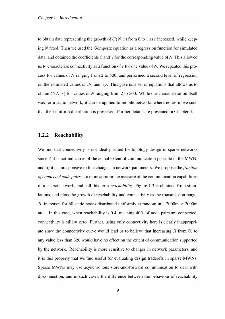
In existing work, MWN topology design has primarily focused on one metric: connectivity.Connectivity is the probability that all the nodes of a network form a single connected component.Most related work consists of asymptotic analyses dealing with finding the values of networkparameters that ensure that the MWN is connected with high probability. The parameters definingthe network are usually the number of nodes, their transmission ranges, and the dimensions of thedeployment area.

In this work, we deal with sparse MWNs, which are unlikely to be completely connected. Weargue that sparse networks can form during the functioning of MWNs, and further, that networkscan be designed to be sparse in order to facilitate tradeoffs between network parameters. Sincemuch existing work on connectivity is asymptotic, and since it focuses only on the operating pointat which the network becomes connected, we provide a finite-domain, empirical model for con-nectivity. However, we find that connectivity is not ideal for dealing with sparse MWNs becauseit is i) not indicative of the extent to which the network supports communication; and ii) it isunresponsive to fine changes in network parameters. We introduce a connectivity property calledreachability, defined as the fraction of connected node pairs in the network, which we claim ismore appropriate for topology design in sparse MWNs. We define and prove properties of reach-ability, and illustrate its application in performing fine-grained tradeoffs in network parametersthrough a case study. We also provide a finite-domain, empirical characterisation of reachability,and a tool called Spanner (Sparse Network Planner) to help apply this model. Given three valuesfrom side of the deployment area, number of nodes, uniform transmission range of the nodes,and reachability, Spanner computes the fourth. Our empirical charecterisations of connectivityand reachability are for static networks with up to 500 nodes uniformly distributed at random in asquare area. These are also applicable to networks with mobile nodes where the mobility modelpreserves the uniform distribution of nodes.

Much work in the area, including our characterisations of connectivity and reachability, arefor networks operating in a square area of deployment. We show that results obtained for a squarearea do not necessarily apply even to similar rectangular areas. We ascribe this to the edge effectby which nodes located near the boundaries of the area of operation cannot utilise their entiretransmission coverage for communication. We quantify analytically the expected coverage for asingle node in a rectangle and describe how this can be applied in extending results obtained forsquare areas to rectangular areas.

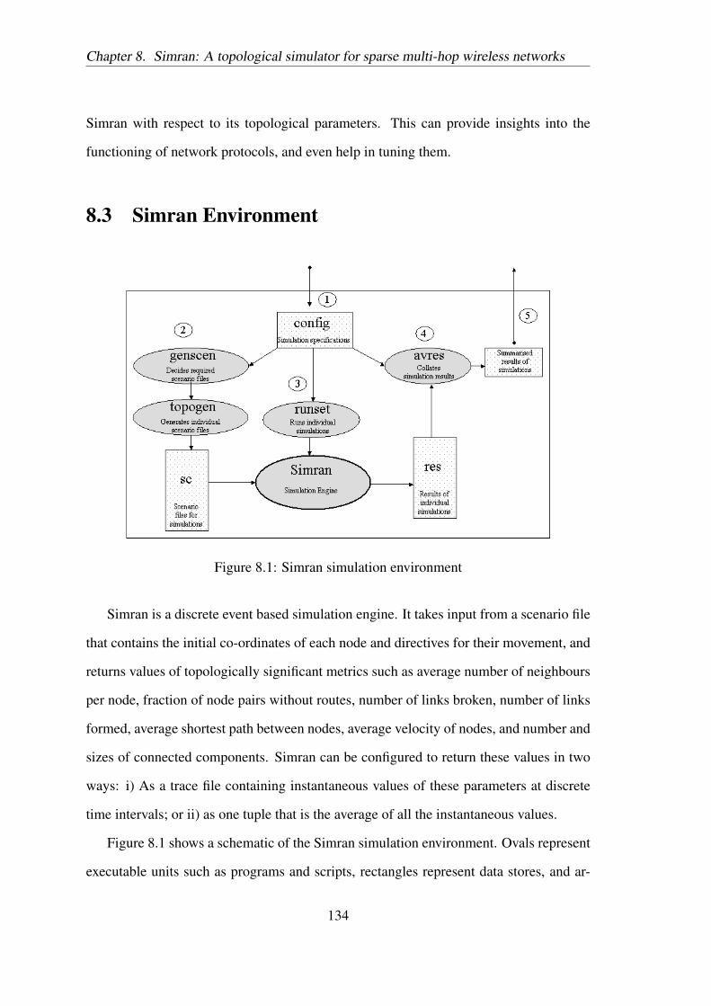
We have also developed a simulator, Simran, for studying topological properties of MWNs.Simran takes as input a scenario file with initial positions and movement traces of nodes, and gen-erates a trace file containing metrics of topological interest such as average number of neighbors,averaged shortest path lengths over all pairs of nodes, reachability, connectivity, and number andsize of connected components.

Contents

1 Introduction 1

1.1 Background . . . . . . . . . . . . . . . . . . . . . . . . . . . . . . . . 3

1.1.1 Topology design . . . . . . . . . . . . . . . . . . . . . . . . . 3

1.1.2 Connectivity properties . . . . . . . . . . . . . . . . . . . . . . 4

1.1.3 Sparse networks . . . . . . . . . . . . . . . . . . . . . . . . . 5

1.2 Overview of work . . . . . . . . . . . . . . . . . . . . . . . . . . . . . 6

1.2.1 Connectivity . . . . . . . . . . . . . . . . . . . . . . . . . . . 8

1.2.2 Reachability . . . . . . . . . . . . . . . . . . . . . . . . . . . 9

1.2.3 Characterising Reachability . . . . . . . . . . . . . . . . . . . 11

1.2.4 Spanner . . . . . . . . . . . . . . . . . . . . . . . . . . . . . . 12

1.2.5 Simran . . . . . . . . . . . . . . . . . . . . . . . . . . . . . . 12

1.2.6 Edge effects in MWNs . . . . . . . . . . . . . . . . . . . . . . 14

1.3 Contributions . . . . . . . . . . . . . . . . . . . . . . . . . . . . . . . 14

1.4 Thesis organisation . . . . . . . . . . . . . . . . . . . . . . . . . . . . 15

2 Related Work and Motivation 17

2.1 Multi-hop Wireless Networks . . . . . . . . . . . . . . . . . . . . . . . 18

2.1.1 Mobile Ad hoc Networks . . . . . . . . . . . . . . . . . . . . . 18

2.1.2 Sensor Networks . . . . . . . . . . . . . . . . . . . . . . . . . 19

2.1.3 Mesh Networks . . . . . . . . . . . . . . . . . . . . . . . . . . 20

iii

Contents

2.2 Connectivity . . . . . . . . . . . . . . . . . . . . . . . . . . . . . . . . 21

2.2.1 The quest for a magic number . . . . . . . . . . . . . . . . . . 22

2.2.2 Critical transmission radius . . . . . . . . . . . . . . . . . . . 23

2.2.3 Finite domain and empirical results . . . . . . . . . . . . . . . 24

2.3 Sparse multi-hop wireless networks . . . . . . . . . . . . . . . . . . . 25

2.3.1 Asynchronous multi-hop wireless networks . . . . . . . . . . . 26

2.4 Reachability . . . . . . . . . . . . . . . . . . . . . . . . . . . . . . . . 27

2.5 Mobility . . . . . . . . . . . . . . . . . . . . . . . . . . . . . . . . . . 29

2.5.1 Mobility models . . . . . . . . . . . . . . . . . . . . . . . . . 29

2.6 Motivation . . . . . . . . . . . . . . . . . . . . . . . . . . . . . . . . . 31

3 Characterising Connectivity 37

3.1 Introduction . . . . . . . . . . . . . . . . . . . . . . . . . . . . . . . . 37

3.1.1 Network model and assumptions . . . . . . . . . . . . . . . . . 38

3.2 Background: Regression analysis . . . . . . . . . . . . . . . . . . . . . 40

3.2.1 Linear Regression . . . . . . . . . . . . . . . . . . . . . . . . 40

3.2.2 Goodness of fit . . . . . . . . . . . . . . . . . . . . . . . . . . 41

3.2.3 Curvilinear Regression . . . . . . . . . . . . . . . . . . . . . . 43

3.3 Characterisation of Connectivity . . . . . . . . . . . . . . . . . . . . . 43

3.4 Details about simulation and curve fitting . . . . . . . . . . . . . . . . 45

3.4.1 How many simulations? . . . . . . . . . . . . . . . . . . . . . 45

3.4.2 Simulations . . . . . . . . . . . . . . . . . . . . . . . . . . . . 48

3.4.3 Regression . . . . . . . . . . . . . . . . . . . . . . . . . . . . 48

3.4.4 Model I . . . . . . . . . . . . . . . . . . . . . . . . . . . . . . 52

3.4.5 Model II . . . . . . . . . . . . . . . . . . . . . . . . . . . . . 53

3.5 Validation . . . . . . . . . . . . . . . . . . . . . . . . . . . . . . . . . 55

3.6 Comparison with other work . . . . . . . . . . . . . . . . . . . . . . . 56

iv

Contents

4 Reachability 59

4.1 Reachability . . . . . . . . . . . . . . . . . . . . . . . . . . . . . . . . 60

4.2 Reachability in mobile and asynchronous MWNs . . . . . . . . . . . . 61

4.2.1 Reachability for mobile MWNs . . . . . . . . . . . . . . . . . 61

4.2.2 Reachability for asynchronous MWNs . . . . . . . . . . . . . . 62

4.2.3 When is a node pair connected? . . . . . . . . . . . . . . . . . 62

4.3 Properties of Reachability . . . . . . . . . . . . . . . . . . . . . . . . . 63

4.4 Applications of reachability . . . . . . . . . . . . . . . . . . . . . . . . 66

4.4.1 Measuring routing performance . . . . . . . . . . . . . . . . . 66

4.4.2 Application: Using reachability for topology design in sparse

MWNs . . . . . . . . . . . . . . . . . . . . . . . . . . . . . . 67

5 Case Study: Reachability for designing a sparse MWN 69

5.1 Case study scenario . . . . . . . . . . . . . . . . . . . . . . . . . . . . 69

5.1.1 Background . . . . . . . . . . . . . . . . . . . . . . . . . . . . 69

5.1.2 A possible MWN solution for intra-village communication . . . 70

5.2 Design Considerations . . . . . . . . . . . . . . . . . . . . . . . . . . 71

5.2.1 Sparse networks . . . . . . . . . . . . . . . . . . . . . . . . . 73

5.3 Deciding deployment parameters . . . . . . . . . . . . . . . . . . . . . 73

5.3.1 Simulation Preliminaries . . . . . . . . . . . . . . . . . . . . . 73

5.3.2 Choosing R . . . . . . . . . . . . . . . . . . . . . . . . . . . . 74

5.3.3 Choosing N . . . . . . . . . . . . . . . . . . . . . . . . . . . . 75

5.3.4 R vs. N . . . . . . . . . . . . . . . . . . . . . . . . . . . . . . 76

5.4 Further observations . . . . . . . . . . . . . . . . . . . . . . . . . . . 77

5.4.1 Network reach . . . . . . . . . . . . . . . . . . . . . . . . . . 77

5.4.2 Mobility . . . . . . . . . . . . . . . . . . . . . . . . . . . . . 78

5.4.3 Asynchronous Communication . . . . . . . . . . . . . . . . . . 79

v

Contents

5.5 Conclusions . . . . . . . . . . . . . . . . . . . . . . . . . . . . . . . . 80

6 Characterising Reachability 81

6.1 Network model and notation . . . . . . . . . . . . . . . . . . . . . . . 82

6.2 Analysis of small cases . . . . . . . . . . . . . . . . . . . . . . . . . . 83

6.2.1 Rch12,r . . . . . . . . . . . . . . . . . . . . . . . . . . . . . . . 83

6.2.2 Rch13,r . . . . . . . . . . . . . . . . . . . . . . . . . . . . . . . 85

6.2.3 Rch13,r without edge effects . . . . . . . . . . . . . . . . . . . 86

6.2.4 Rch13,r with edge effects . . . . . . . . . . . . . . . . . . . . . 93

6.3 Modelling RchN,r in the finite domain . . . . . . . . . . . . . . . . . . 102

6.4 Empirical modelling of RchN,r in the finite domain . . . . . . . . . . . 103

6.4.1 The Logistic Growth Curve . . . . . . . . . . . . . . . . . . . 103

6.5 Simulation and Regression Modelling . . . . . . . . . . . . . . . . . . 104

6.5.1 Simulations . . . . . . . . . . . . . . . . . . . . . . . . . . . . 105

6.5.2 Fitting the Logistic Curve . . . . . . . . . . . . . . . . . . . . 106

6.5.3 Fitting the Logistic Coefficients . . . . . . . . . . . . . . . . . 107

6.5.4 Validation . . . . . . . . . . . . . . . . . . . . . . . . . . . . . 109

6.6 Extending the model . . . . . . . . . . . . . . . . . . . . . . . . . . . 110

6.7 Using the model: Spanner . . . . . . . . . . . . . . . . . . . . . . . . 111

6.8 Handling model limitations . . . . . . . . . . . . . . . . . . . . . . . . 112

6.8.1 Idealised wireless propagation . . . . . . . . . . . . . . . . . . 112

6.8.2 Square area of operation . . . . . . . . . . . . . . . . . . . . . 112

6.8.3 Mobility . . . . . . . . . . . . . . . . . . . . . . . . . . . . . 113

6.9 Concluding remarks . . . . . . . . . . . . . . . . . . . . . . . . . . . . 114

7 Edge effects on Connectivity Properties 117

7.1 Motivation . . . . . . . . . . . . . . . . . . . . . . . . . . . . . . . . . 117

7.2 Quantifying the edge effect for a single node . . . . . . . . . . . . . . . 119

vi

Contents

7.2.1 Coverage in Region 1 . . . . . . . . . . . . . . . . . . . . . . . 121



7.2.4 Combined expected coverage for the three regions . . . . . . . 125

7.2.5 Connectivity: C2,r . . . . . . . . . . . . . . . . . . . . . . . . 125

7.3 Applying our formula for edge effects . . . . . . . . . . . . . . . . . . 126

7.3.1 How to square a rectangle . . . . . . . . . . . . . . . . . . . . 127

8 Simran: A topological simulator for sparse multi-hop wireless networks 131

8.1 Introduction . . . . . . . . . . . . . . . . . . . . . . . . . . . . . . . . 131

8.2 Motivation and Design considerations . . . . . . . . . . . . . . . . . . 132

8.3 Simran Environment . . . . . . . . . . . . . . . . . . . . . . . . . . . 134

8.4 Simran . . . . . . . . . . . . . . . . . . . . . . . . . . . . . . . . . . . 136

8.4.1 Implementation . . . . . . . . . . . . . . . . . . . . . . . . . . 137

8.4.2 Scalability and Complexity . . . . . . . . . . . . . . . . . . . . 139

8.5 Handling asynchronous communication . . . . . . . . . . . . . . . . . 142

8.6 Illustrative example . . . . . . . . . . . . . . . . . . . . . . . . . . . . 144

9 Conclusion 147

9.1 Limitations of our work . . . . . . . . . . . . . . . . . . . . . . . . . . 148

9.2 Future directions for work . . . . . . . . . . . . . . . . . . . . . . . . 149

9.2.1 Analytical results for connectivity properties . . . . . . . . . . 149

9.2.2 Three dimensional networks . . . . . . . . . . . . . . . . . . . 150

9.2.3 Simulation techniques . . . . . . . . . . . . . . . . . . . . . . 150

9.3 Publications . . . . . . . . . . . . . . . . . . . . . . . . . . . . . . . . 153

vii

List of Figures

1.1 Different network instances of the same network . . . . . . . . . . . . 4

1.2 Connectivity vs. Normalised transmission range . . . . . . . . . . . . . 8

1.3 Increasing R, no mobility . . . . . . . . . . . . . . . . . . . . . . . . . 10

1.4 Increasing R, with mobility and asynchronous communication . . . . . 10

1.5 Determining R and N for a given reachability . . . . . . . . . . . . . . 12

1.6 Simran simulation environment . . . . . . . . . . . . . . . . . . . . . . 13

3.1 Connectivity vs. Normalised transmission range . . . . . . . . . . . . . 38

3.2 Standard Deviation vs. Connectivity for 90 nodes . . . . . . . . . . . . 45

3.3 Linear fit for F vs. r for N = 30 . . . . . . . . . . . . . . . . . . . . . 50

3.4 βN vs. N . . . . . . . . . . . . . . . . . . . . . . . . . . . . . . . . . . 52

3.5 γN vs. N . . . . . . . . . . . . . . . . . . . . . . . . . . . . . . . . . . 53

3.6 eβN vs. N, 3 ≤ N < 130 . . . . . . . . . . . . . . . . . . . . . . . . . 54

3.7 eβN vs. N, 130 ≤ N ≤ 500 . . . . . . . . . . . . . . . . . . . . . . . . 55

4.1 Increasing R, no mobility . . . . . . . . . . . . . . . . . . . . . . . . . 60

4.2 A network instance with Reachability = 0.378 . . . . . . . . . . . . . . 61

5.1 Reachability and Connectivity vs. R . . . . . . . . . . . . . . . . . . . 74

5.2 Reachability and Connectivity vs. N . . . . . . . . . . . . . . . . . . . 75

5.3 Determining R and N for a given reachability . . . . . . . . . . . . . . 76

ix

List of Figures

5.4 With asynchronous communication . . . . . . . . . . . . . . . . . . . . 79

6.1 Positions of a single node on a line segment . . . . . . . . . . . . . . . 83

6.2 Tree diagram of outcomes for three nodes positioned on a line . . . . . 87

6.3 Case X: N2 is connected to N1 . . . . . . . . . . . . . . . . . . . . . . 88

6.4 Case Y : N2 can only connect to N1 through an intermediate node . . . 89

6.5 Case Z: N2 cannot connect to N1 even through an intermediate node . . 91

6.6 A general logistic curve . . . . . . . . . . . . . . . . . . . . . . . . . . 104

6.7 Logistic fit for N=100 . . . . . . . . . . . . . . . . . . . . . . . . . . . 105

6.8 Estimated and fitted α . . . . . . . . . . . . . . . . . . . . . . . . . . . 108

6.9 Estimated and fitted β . . . . . . . . . . . . . . . . . . . . . . . . . . . 109

7.1 Connectivity properties change with rectangularity . . . . . . . . . . . 119

7.2 Edge effects on a node’s radio coverage . . . . . . . . . . . . . . . . . 120

7.3 Edge effect in Region 2 . . . . . . . . . . . . . . . . . . . . . . . . . . 121

7.4 Edge effects in Region 3 . . . . . . . . . . . . . . . . . . . . . . . . . 123

8.1 Simran simulation environment . . . . . . . . . . . . . . . . . . . . . . 134

8.2 Screen shots of the Simran environment . . . . . . . . . . . . . . . . . 145

x

List of Tables

2.1 Network parameters from 60 MobiHoc papers, 2001-2005 . . . . . . . 34

3.1 Simulated Data for N=30 . . . . . . . . . . . . . . . . . . . . . . . . . 49

3.2 Simulated Data for N=300 . . . . . . . . . . . . . . . . . . . . . . . . 49

3.3 N, βN , γN and R2 . . . . . . . . . . . . . . . . . . . . . . . . . . . . . 51

3.4 Comparison of Models . . . . . . . . . . . . . . . . . . . . . . . . . . 57

6.1 Analytical and Simulated values for r = 0.1 . . . . . . . . . . . . . . . 101

6.2 N = 60 . . . . . . . . . . . . . . . . . . . . . . . . . . . . . . . . . . 107

6.3 N with corresponding α and β . . . . . . . . . . . . . . . . . . . . . . 107

6.4 Beyond N = 500 . . . . . . . . . . . . . . . . . . . . . . . . . . . . . 111

7.1 C2,r: simulated and analytical . . . . . . . . . . . . . . . . . . . . . . . 126

xi

Chapter 1

Introduction

Multi-hop Wireless Networks (MWNs) are decentralised, infrastructure-less networks

enabled by cooperative multi-hop routing among the participating nodes. In recent years

there has been much work on MWNs, and this has shown their applicability for diverse

uses: Mobile ad hoc networks (MANETs) can be used for communication where net-

work infrastructure may be unavailable, such as in vehicular networks or in battlefield

and disaster relief operations; sensor networks have been used for collaborative sens-

ing of events in inaccessible or dangerous areas; and mesh networks have been used for

economical deployment of multi-hop backbone infrastructure for community and neigh-

bourhood networks.

An important aspect of deploying MWNs is the topology design of the network.

Topology design deals with deciding what values network parameters such as number

of nodes or transmission power of radios should take in order to meet a design objective.

Typical design objectives of topology design could be to ensure that the network is con-

nected, that is, every node in the network has a path to every other node in the network,

or to ensure that a specified network throughput is achievable.

Much existing work on MWNs has taken the view that a network needs to be con-

nected in order to be useful. We have identified sparse MWNs as a class of MWNs in

1

Chapter 1. Introduction

which the network may not be fully connected. Such networks can easily arise during

the operation of an MWN. For example, a vehicular ad hoc network can become sparse

when traffic density is low. Or, a sensor network may become sparse after the failure

of some of its nodes. Moreover, we found that sparse MWNs can often support a sig-

nificant amount of communication. This leads to the interesting possibility that MWNs

can be designed to be sparse in order to facilitate tradeoffs between network parameters,

deployment cost and its connectivity properties. A connectivity property is a measure

of the extent to which a network possesses paths between its nodes. This thesis studies

topology design for sparse multi-hop wireless networks with respect to their connectivity

properties.

We are interested in answering questions such as:

• Are currently used connectivity properties appropriate for topology design in sparse

MWNs?

– If so, how can they be used?

– If not, what other connectivity properties can be used?

• What is the nature of tradeoffs between network parameters that can be made in

sparse deployments?

• What tools, such as models or simulators, would we require in order to accomplish

such tradeoffs?

The answers to these and related questions form the body of this thesis, of which we

provide an overview in Section 1.2. But we first give a more detailed introduction to

topology design, connectivity properties and sparse networks.

2


1.1 Background

1.1.1 Topology design

Topology design is an important concern in deploying MWNs since it determines the

extent to which a network can support communication. An MWN topology is charac-

terised by its network graph, which in turn depends on physical network parameters such

as number of nodes, transmission range of nodes, area of the network’s operation, and

type and extent of mobility. To illustrate, if the transmission range of nodes in a network

is increased with all other parameters retaining their value, the average node degree of the

network graph increases, and the number of hops on multi-hop paths decreases. Similar

effects can be seen on the network graph by decreasing the area of operation. In gen-

eral, topology design involves setting network parameters such that the network graph

that is obtained is suitable with respect to the constraints and intended application of the

network.

A network is characterised by its parameters—in this thesis the parameters we choose

are the number of nodes N , their uniform transmission range R, the dimensions of the

network’s area of operation D, and location and mobility model parameters M . There-

fore, a network, for our purposes, can be defined as a tuple: < N,R,D,M >. Further,

we state that the nodes of the network are initially located at positions chosen uniformly

at random within the operational area. It is important to make the distinction here be-

tween a network and a network instance. That is, the same network parameters can result

in different network graphs depending on the specific locations that the nodes take. To

illustrate, if an MWN defined by < N,R,D,M > is to be deployed by scattering nodes

over a field, two deployments could have different network graphs even though the net-

work parameters are the same. For example, Figure 1.1 shows two instances of a network

of 9 nodes, each with a transmission range of 100m, in a 500m× 500m area.

Note that topology design for a network instance can be deterministic. That is, we

3


can set values of network parameters for each node such that the exact desired topology

is obtained. (This is commonly done with mesh networks, for example, where mesh

nodes are installed at pre-determined locations.) But for a randomly deployed network

defined only by its network parameters, topology design is usually probabilistic, and the

objectives for topology design are met with some probability.

Topology design can be performed towards several objectives. For example, we may

want to control the number of hops along a multi-hop path; or, we may want to adjust

network parameters such that the network graph remains connected, but is not of such

high degree that there is a significant loss of throughput due to radio interference. In this

thesis, we are concerned with topology design with respect to the network’s connectivity

properties.

Figure 1.1: Different network instances of the same network

1.1.2 Connectivity properties

A connectivity property is a value associated with a network or a network instance that

indicates the extent to which the nodes in the network are connected by paths. A well-

studied example of a connectivity property in the context of MWNs is called connectiv-

ity. A network instance is said to be connected when all its nodes are part of a single

4


connected component. (For example, in Figure 1.1, the network instance on the left is

connected.) We use the following definition of connectivity: connectivity of a network is

the probability of a network instance being connected. Other examples of connectivity

properties include the size of the largest connected component of the network graph, and

reachability, introduced later in this thesis, and defined as the fraction of connected node

pairs in the network.

1.1.3 Sparse networks

In this thesis, we deal with sparse MWNs. A sparse MWN is one which does not form

a single connected component, or one in which connectivity with high probability is not

ensured. We define a sparse network as follows: An MWN is sparse if its probability of

being connected is less than 0.95.

A sparse network can arise in various ways: a vehicular ad hoc network in an area

with low traffic density, an initially connected sensor network after some of its nodes

have failed, and an ad hoc communications network that is being deployed incrementally

can all be sparse networks. In constrained deployment scenarios, we may even wish to

deploy a multi-hop network that trades off connectivity for deployment cost. There is

work [SB03] that shows that tolerating some sparseness (requiring only 90% of nodes

to be in the same connected component) results in a significant reduction in the required

transmission range of nodes.

To examine the prevalence of sparse networks in MWN studies, we considered net-

work parameters used for simulations in papers presented at the MobiHoc conference

from the years 2000 to 2005 (the parameters are tabulated in [KCC05]). We conducted

simulations to determine the connectivity of each set of network parameters, and classi-

fied a network as sparse if its connectivity was less than 0.95. This classification is in

5


Table 2.1 in Chapter 2, and shows that 25 of the 60 networks examined were sparse.

1.2 Overview of work

We had raised the following questions as being of interest:

• Are currently used connectivity properties appropriate for topology design in sparse

MWNs?

– If so, how can they be used?

– If not, what other connectivity properties can be used?

• What is the nature of tradeoffs between network parameters that can be made in

sparse deployments?

• What tools, such as models or simulators, would we require in order to accomplish

such tradeoffs?

We went about answering them as follows.

We first considered applying connectivity for topology design in sparse MWNs. We

found that most existing work on connectivity (covered in Section 2.2) attempts to find

the relation between network parameters such that the resulting MWN is connected with

high probability. In contrast, topology design in sparse networks requires a continu-

ous characterisation of connectivity that would express the network’s capabilities across

a range of network parameters. Further, most existing results are asymptotic and are

difficult to apply to sparse networks. We therefore obtained a finite domain, empiri-

cal characterisation of connectivity in terms of number of nodes and transmission range

normalised with the area of operation.

6


We found that the connectivity metric itself can be unsuitable when applied to sparse

networks since i) it does not indicate the actual extent of communication possible in the

MWN; and ii) it is unresponsive to fine changes in network parameters. We proposed that

the fraction of connected node pairs, which we call reachability, would be a more appro-

priate measure for topology design in sparse networks, and proved its properties that are

useful for this purpose. We also performed a case study showing how to apply reacha-

bility for evaluating design tradeoffs in sparse MWNs, and performed a characterisation

which we incorporated into a design tool.

We also developed a simulator for studying topological properties of MWNs. This

simulator, called Simran, takes as input a scenario file with initial positions and move-

ment scripts of nodes, and generates a trace file containing metrics of interest such as

average number of neighbour, averaged shortest path lengths over all pairs of nodes,

reachability, connectivity, and number and size of connected components.

We found that our characterisations of reachability and connectivity, and much ex-

isting work in the area of topology design, give results for networks operating in square

areas. However, results obtained for a square area did not necessarily apply even to sim-

ilar rectangular areas. We attributed this to the edge effect where nodes at the boundaries

of the area of operation do not use their full coverage area for communication. We ana-

lytically quantified the edge effect and obtained a method to extend connectivity property

related results for square areas to a more general rectangular area.

We now present a more detailed overview of our work. The network model we used

for our characterisations is as follows: N nodes, each with a transmission range of R are

distributed uniformly at random in a square area of side l; r = R/l is the normalised

transmission range. We represent connectivity, modelled as a function of N and r, as

C(N, r), and reachability as Rch(N, r).

7


1.2.1 Connectivity

Most studies of connectivity (summarised in Section 2.2) have been asymptotic analyses

of probabilistic connectivity, and become accurate as the number of nodes in the network

increases. Some studies make use of the property that for large numbers of nodes, the

connectivity versus transmission range curve behaves like a step function: at a critical

value of transmission range, connectivity rises rapidly from almost zero to almost one

[KWB01]. This property is made use of to analyse the point at which this transition

occurs. As seen in Figure 1.2, such threshold behaviour, and in turn analyses based

on this property, may not be accurately applicable to smaller networks with tens or a few

hundreds of nodes. Further, we are specifically interested in the behaviour of connectivity

properties in sparse MWNs. Such networks, by definition, are not fully connected, and

our interest lies more in in finding exact values of connectivity for different combinations

of number of nodes, transmission ranges and operational areas, than in determining when

the network is fully connected. We obtain a finite domain, empirical characterisation of

connectivity suitable for applying to sparse MWNs.

Figure 1.2: Connectivity vs. Normalised transmission range

We explored data from comprehensive simulations, and found that C(N, r) fits the

Gompertz equation in the form: C(N, r) = e−e(βN−γNr) . We then conducted simulations

8


to obtain data representing the growth of C(N, r) from 0 to 1 as r increased, while keep-

ing N fixed. Then we used the Gompertz equation as a regression function for simulated

data, and obtained the coefficients β and γ for the corresponding value of N. This allowed

us to characterise connectivity as a function of r for one value of N. We repeated this pro-

cess for values of N ranging from 2 to 500, and performed a second level of regression

on the estimated values of βN and γN . This gave us a set of equations that allows us to

obtain C(N, r) for values of N ranging from 2 to 500. While our characterisation itself

was for a static network, it can be applied to mobile networks where nodes move such

that their uniform distribution is preserved. Further details are presented in Chapter 3.

1.2.2 Reachability

We find that connectivity is not ideally suited for topology design in sparse networks

since i) it is not indicative of the actual extent of communication possible in the MWN;

and ii) it is unresponsive to fine changes in network parameters. We propose the fraction

of connected node pairs as a more appropriate measure of the communication capabilities

of a sparse network, and call this term reachability. Figure 1.3 is obtained from simu-

lations, and plots the growth of reachability and connectivity as the transmission range,

R, increases for 60 static nodes distributed uniformly at random in a 2000m × 2000m

area. In this case, when reachability is 0.4, meaning 40% of node pairs are connected,

connectivity is still at zero. Further, using only connectivity here is clearly inappropri-

ate since the connectivity curve would lead us to believe that increasing R from 50 to

any value less than 320 would have no effect on the extent of communication supported

by the network. Reachability is more sensitive to changes in network parameters, and

it is this property that we find useful for evaluating design tradeoffs in sparse MWNs.

Sparse MWNs may use asynchronous store-and-forward communication to deal with

disconnection, and in such cases, the difference between the behaviour of reachability

9


and connectivity is accentuated. Figure 1.4 is for a network where a node can store and

forward data for another node for up to 30 seconds. In this case, almost 80% of node

pairs have a path connecting them before connectivity rises above zero.

Figure 1.3: Increasing R, no mobility

The reachability of a static network is defined as the fraction of connected node pairs

in the network. Using this definition we can calculate reachability for a network of N

nodes as1:

Reachability =No. of connected node pairs(

N2

) (1.1)

Figure 1.4: Increasing R, with mobility and asynchronous communication

We identify the following properties of reachability:

1We assume that communication links between nodes are symmetric.

10


1. The reachability of a network lies in the interval [0, 1].

2. Reachability of a network is not less than the connectivity of the same network.

3. Reachability represents the probability that there exists a path between a randomly

chosen pair of nodes in an MWN.

4. Reachability of a network represents the long term maximal packet delivery ratio

achievable between random source-destination pairs in the network.

We prove these properties and describe the application of Property 4 in measuring routing

performance in sparse MWNs in Chapter 4. The use of reachability for topology design

is illustrated through a case study in Chapter 5.

1.2.3 Characterising Reachability

It may be possible to obtain asymptotic bounds for reachability, but since sparse networks

often involve small numbers of nodes, we are particularly interested in characterisations

in the finite domain, and we chose to model reachability using empirical regression. We

model reachability as a function of N and r, and denote it by Rch(N, r).

For the characterisation, we explored data from comprehensive simulations and found

that Rch(N, r) obeys logistic growth as given by Rch(N, r) = 11+eαN−βNr

. We then

conducted extensive simulations to obtain data that represented the growth of Rch(N, r)

from 0 to 1 as r increased, while keeping N fixed. We then used the logistic equation

as a regression function, and obtained the coefficients α and β for the corresponding

value of N. This allowed us to characterise reachability as a function of r for one value

of N. We repeated this process for values of N ranging from 2 to 500, and performed

a second level of regression on the estimated values of αN and βN . This gave us a set

of equations that allows us to obtain Rch(N, r) for values of N ranging from 2 to 500.

11


While our characterisation was for a static network, it can be applied to mobile networks

where nodes move such that their uniform distribution is preserved. Further details are

presented in Chapter 6.

1.2.4 Spanner

Spanner2 is a tool we have developed for topology design in sparse MWNs. It uses our

empirical model for reachability. It takes as input any three values from number of nodes,

side of the deployment area, uniform transmission range of the nodes, and reachability,

and computes the fourth value. As an example of Spanner’s use, Figure 1.5 is plotted

from data generated by Spanner, and shows the tradeoff required between number of

nodes and transmission range to maintain a desired value of reachability. More details

about Spanner can be found in Section 6.7.

Figure 1.5: Determining R and N for a given reachability

1.2.5 Simran

Simran3 is a simulator we have developed for studying topological properties of MWNs.

Simran takes as input a scenario file with initial positions and movement scripts of nodes,

2Sparse network planner: http://www.it.iitb.ac.in/∼srinath/tool/rch.html3Available from http://www.it.iitb.ac.in/∼srinath/simran/

12


Figure 1.6: Simran simulation environment

and generates a trace file containing metrics of interest such as average number of neigh-

bour, averaged shortest path lengths over all pairs of nodes, reachability, connectivity,

and number and size of connected components. Simran is also supported by a number

of smaller programs for generating scenario files, managing large simulations, and for

analysing results. A schematic diagram of the Simran simulation environment is shown

in Figure 1.6. Simran can be used to evaluate design tradeoffs in sparse MWNs: Figures

1.3 and 1.4 are generated from results of simulations in Simran. Further, all data used for

the characterisation of reachability and connectivity were also generated using Simran.

Simran also supports topological simulation of networks with asynchronous communica-

tion. To facilitate simulation of asynchronous networks, we have modified the transitive

closure algorithm to operate across multiple adjacency matrices representing the network

at different instants. We call this the Temporal Transitive Closure algorithm. More details

about this algorithm, and the design, implementation and use of Simran, can be found in

Chapter 8.

13


1.2.6 Edge effects in MWNs

The empirical models presented in this thesis for connectivity and reachability are for

nodes in a square area of operation. While the assumption of a square area of operation

is common in work relating to connectivity properties of multi-hop networks, it is not

clear how analytical or empirical results obtained for a square area can be applied to a

more general rectangular area. We show that results obtained for a square area do not

necessarily apply even to similar rectangular areas: we present simulation results that

show reachability and connectivity varying for networks with the same area of operation,

but with differing geometries. We ascribe this to the edge effect by which nodes located

near the boundaries of the area of operation cannot utilise their entire transmission cov-

erage for communication. This edge effect varies with the shape of the operating area,

thereby also changing values of connectivity properties for the MWN. We quantify ana-

lytically the expected coverage for a single node in a rectangle and describe how this can

be applied in extending results obtained for square areas to rectangular areas. Details are

presented in chapter 7.

1.3 Contributions

The main contributions of this thesis are:

• an empirical model for connectivity for a two-dimensional network in the finite

domain that is more general, accurate, and simpler to use than existing models for

topology design in networks up to 500 nodes;

• identifying reachability as a suitable connectivity property for topology design in

sparse MWNs, and properties of reachability that are useful towards this end;

• demonstrating the use of reachability for topology design and measuring routing

protocol performance in sparse MWNs;

14


• an empirical, finite domain model for reachability of a two-dimensional network;

• Spanner: a topology design tool for sparse MWNs;

• Simran: a topological simulator for multi-hop wireless networks that is suitable for

studying sparse networks; and

• quantification of the boundary effect for a single node in two dimensions, and

its application in generalising results for connectivity properties in MWNs from

square areas to more general rectangular areas.

1.4 Thesis organisation

We present related work in the area of MWNs in general, and in the area of topology

design and sparse networks in particular, and motivate our work in relation to it in Chapter

2. Chapter 3 describes our characterisation of connectivity for MWNs. We introduce

the notion of reachability, its definition, properties, and applications in Chapter 4. In

Chapter 5, we illustrate the use of reachability for topology design in sparse MWNs

with a case study. An empirical characterisation of reachability, and our attempts at

an analytical characterisation are presented in Chapter 6. In the same chapter, we also

describe Spanner, a tool we have developed for topology design in sparse networks based

on our empirical model for reachability. In Chapter 7, we analyse the extent of the

edge effect for a single node in an MWN, and describe its use in generalising results

for connectivity properties from square to rectangular areas. We describe the design and

implementation of Simran, our topological simulator, in Chapter 8. In the same chapter,

we also present the Temporal Transitive Closure algorithm used in Simran for simulating

asynchronous networks. We end with concluding remarks in Chapter 9.

15


16

Chapter 2

Related Work and Motivation

The main theme of this thesis is topology design of sparse Multi-hop Wireless Networks

(MWNs) with emphasis on connectivity properties. The term MWNs is a broad one,

encompassing mobile ad hoc networks, sensor networks and mesh networks. In Section

2.1 we present a brief overview of MWNs and their types, and outline characteristic

research issues for these networks.

A connectivity property that has been very widely used in the context of MWNs is

connectivity. In Section 2.2 we define connectivity and present an overview of existing

work. We are specifically interested in sparse MWNs, and work related to sparse MWNs

is summarised in Section 2.3. In this thesis we claim that connectivity is not suitable for

topology design in sparse MWNs, and we propose a metric called reachability. Though

there has been no thorough study of reachability, the notion has been touched upon briefly

by others using different terms. We summarise existing work on reachability in Section

2.4. MWNs are often mobile. Section 2.5 briefly discusses the effect of mobility on

such networks, and gives an overview of mobility models used or referenced later in this

thesis. We conclude this chapter with Section 2.6 by relating the work in this thesis to

the existing work discussed in this chapter.

17

Chapter 2. Related Work and Motivation

2.1 Multi-hop Wireless Networks

Multi-hop Wireless Networks (MWNs) are decentralised, infrastructure-less networks

enabled by cooperative multi-hop routing among the participating nodes, and have been

the subject of much work in recent years. One reason for this recent interest is the increas-

ing availability of smaller, cheaper and more powerful mobile devices with improved

wireless networking capabilities. Using multi-hop wireless transmission is attractive be-

cause for a given distance, the total power required to transmit a packet is lower over

multiple hops than for a single hop. Further, this lower transmission power reduces the

extent of radio interference and allows parallel streams of communication in the network.

Multi-hop wireless Networks can be divided based on application into the following

kinds of networks: Mobile Ad hoc Networking (MANET), Sensor Networks and Mesh

Networks. Each of these types of networks have their own characteristic issues and are

thriving areas of research.

2.1.1 Mobile Ad hoc Networks

A MANET is a collection of mobile nodes with wireless capabilities in which each node

can act as a router. Nodes communicate using a multi-hop path in which other nodes of

the MANET act as intermediate nodes. Typically MANETs do not rely on any infrastruc-

ture outside the nodes themselves. Often cited application scenarios include battlefield

communications and disaster relief operations where networking infrastructure may be

unavailable or destroyed. Active research issues in MANETs are medium access, trans-

port layer performance, quality of service, security and applications. Chlamtac and oth-

ers present a comprehensive survey of advances and challenges in MANET research in

[CCL02].

A characteristic issue in MANETs is routing. It is particularly challenging and inter-

esting since nodes are mobile. Even after a multi-hop route is discovered from source

18


to destination, it can be broken by the movement of any of the intermediate nodes along

the route. A large number of MANET routing protocols have been proposed to address

the issues of route discovery and maintenance. Broadly, these can be classified as being

proactive or reactive. In proactive protocols, each node maintains at all times a route

from itself to every other node in the network. An example of a proactive MANET rout-

ing protocol is DSDV (Destination Sequenced Distance Vector), which extends distance

vector routing to MANETs by introducing more frequent updates to handle mobility,

and a destination sequence number to avoid routing loops. Popular reactive protocols

are DSR (Dynamic Source Routing) [JM96] and Ad hoc On-demand Distance Vector

(AODV) [DPR00] which discover routes when there is a packet to be sent. Both DSR

and AODV discover routes by having the source flood the network with route discovery

packets, and having the destination reply with the sequence of hops required to reach it.

DSR performs source routing and appends this route to each packet, while AODV main-

tains routing tables at each intermediate node which contain next-hop information for

the route. There are also hybrid, hierarchical and location-aided approaches to routing in

MANETs. A comprehensive survey of MANET routing strategies is available in [BR03].

Almost all the work in this thesis is directly applicable to MANETs: our simulator,

Simran, described in Chapter 8 can be used for simulating topological properties of dense

and sparse MANETs; our connectivity and reachability characterisations can be used

for topology design of MANETs, that is, they help choose network parameters such as

number of nodes and transmission range that result in desired values of connectivity

properties.

2.1.2 Sensor Networks

A typical sensor network consists of a large number of nodes which are capable of sens-

ing some phenomenon of interest and communicating this information to a central base

19


station. Akyilidz and others present a survey of issues and research in the sensor network

area in [ASSC02].

Sensor networks can be deployed where human presence may be inconvenient or im-

possible. Typical applications include sensing the presence of hazardous materials in a

chemical plant, and identifying and communicating sources of threat in a battlefield sce-

nario. Since random deployment of sensor nodes may be required, sensor network pro-

tocols must support self-organisation. Much research has gone into developing schemes

that allow for low-power operation of sensor networks. These schemes include using

sleep and wake-up schedules to minimise the time a node’s radio is operational, and data

filtering and aggregation to ensure that radio transmissions are as few as possible. Sen-

sor networks are usually more dense than MANETs or mesh networks, and data may be

transmitted using a large number of hops to save power. Routing in such networks is

typically data-centric as opposed to node-centric in other forms of MWNs.

Much of the work in this thesis can be applied to sensor networks: Simran supports

topological simulations in sensor networks, and the characterisation of connectivity can

be used to determine network parameters such as number of nodes and transmission

range required for complete or partial connectivity. Our characterisation of reachability

can be used for topology design when sensor nodes are mobile.

2.1.3 Mesh Networks

Wireless mesh networks are MWNs that function as backbone networks for a set of

clients. Akyilidz and others survey advances and challenges in the area of mesh net-

working in [AWW05].

Mesh networks consist of several mesh routers each of which may have multiple

wireless links to connect to other mesh routers and clients. Mesh routers can also act

as gateways by allowing clients to connect to them using a variety of network technolo-

20


gies such as Ethernet, 802.11, or a cellular network. Mesh networks can be an effective

last-mile solution where the terrain is difficult, or where adequate infrastructure does not

exist. Since such a solution can be deployed incrementally, and can be developed using

inexpensive hardware, mesh networks are also cost effective, and are popular for set-

ting up community and neighbourhood networks. Typically mesh routers are not mobile

and routing is not as challenging as for MANETs. But mesh networks do need to be

self-organising and adaptive to some extent to handle router failures and client mobility.

Many existing mesh networks use well-established MANET routing protocols or their

variants. Since mesh networks act as a backbone, network availability and capacity are

of prime importance, and there is much work in this area. The operation and scheduling

of multiple radio transceivers on mesh routers is also an active area of research.

The work in this thesis is primarily applicable when nodes are distributed randomly.

While that is often the case with MANETs and sensor networks, mesh nodes are usually

positioned in a carefully designed topology. However, our simulator Simran, can be

used with mesh networks to determine topological properties of the network such as

connectivity, number of neighbours per node, and shortest path lengths, which are useful

in designing mesh networks, particularly those with large numbers of nodes.

2.2 Connectivity

A network graph is said to be connected when all its nodes belong to a single con-

nected component. Traditionally, MWNs have been regarded as useful when they are

fully connected, that is, when all the nodes in the network are part of a single connected

component, and topology design efforts have therefore concentrated on determining the

conditions under which the network becomes fully connected. Given network param-

eters such as the number of nodes, their distribution and their transmission ranges, the

connectivity metric is usually defined as the probability that the network forms a single

21


connected component.

There is much work on finding the ‘magic number’ of neighbours per node that

ensures connectivity, and we summarise this work in Section 2.2.1. Work addressing

the Critical Transmission Range (CTR) problem, which finds the transmission range of

nodes for which the network is connected with high probability, is covered in Section

2.2.2. Most work on these problems have involved asymptotic analyses. There also exist

analytical and empirical results characterising connectivity in the finite domain and we

present these in Section 2.2.3. This last mentioned work is directly related to ours: In

Chapter 3 we present an empirical, finite domain characterisation for connectivity for use

with sparse networks.

2.2.1 The quest for a magic number

In a multi-hop network, the transmission ranges of the nodes plays an important part in

establishing both the connectivity and the capacity of the resulting network. If the trans-

mission range is too low, the degree of nodes in the network graph may be too low for it

to be connected, and nodes may be isolated. If the range is too high, the network graph

has nodes with larger degree, and nodes are more likely to interfere with each others’

transmissions. While this decreases network capacity, an additional factor to be consid-

ered is that a larger node degree decreases the number of transmission hops required from

source to destination. This was formulated as an optimisation problem in Kleinrock and

Silvester’s 1978 paper titled ‘Optimum Transmission Radii for Packet Radio Networks

or Why Six is a Magic Number’ [KS78]. They found that the optimum transmission

radius which maximises throughput in a slotted ALOHA packet radio network resulted

in around six neighbours per node.

Much work followed Kleinrock and Silvester’s result identifying six as a magic num-

ber. In a subsequent paper, Takagi and Kleinrock revised this magic number to eight

22


for slotted ALOHA, and identified magic numbers when the transmission protocols used

were CSMA (Carrier Sense Multiple Access) and slotted ALOHA with capture as five

and seven respectively[TK84]. Other work using different transmission strategies came

up with magic numbers of six and eight [HL86], and three [Haj83]. Royer and others

performed simulation studies for a mobile ad hoc network running the AODV routing

protocol and found the optimal number of neighbours to be between seven and eight, and

further that this number increased with mobility [RMSM01].

In 2004, Xue and Kumar showed that a multi-hop network is asymptotically discon-

nected with probability one if each node is connected to less than 0.074 lnn neighbours,

and asymptotically connected with probability one if each node is connected to more

than 5.1774 lnn neighbours. Therefore, there cannot exist a single magic number as a

multi-hop network grows arbitrarily large [XK04].

2.2.2 Critical transmission radius

It is known that for large numbers of nodes, the connectivity versus transmission range

curve behaves like a step function: at a critical value of transmission range, connectivity

rises rapidly from almost zero to almost one [KWB01]. There is work in the asymptotic

domain to find the Critical Transmission Radius (CTR) that guarantees that the network

is completely connected.

Gupta and Kumar have shown using the theory of continuum percolation that a net-

work with n nodes on a disc of unit area is almost surely connected if the transmission

range is O(√

(lnn+ c(n))/n) with c(n)→∞ as n→∞ [GK98, KMK04].

Santi and Blough have used occupancy theory to analyse the CTR for multi-hop wire-

less networks [SB02, SBV01, SB03]. They obtain bounds for one dimensional networks

as follows: For n nodes of transmission range r distributed uniformly as random on a line

of length l, the communication graph is connected with high probability if rn ∈ Θ(l ln l),

23


while it is not if rn ∈ O(l). They go on to show that if rn = k ln l, the network is

connected w.h.p. when k ≥ 2 and not connected w.h.p. when k < 1. They also provide a

lower bound for the CTR in two and three dimensional networks: in d dimensions, with

n � 1 and r � l, the network is not connected w.h.p. when r2n ∈ O(l2). A difference

in their work from Gupta and Kumar’s is that they explicitly use the length of the side of

the operating area l in their analyses, rather than working with only node density. As a

result, their work is applicable even in networks with low node densities. However, it is

asymptotic in the number of nodes.

Most existing work on the CTR problem uses an idealised radio propagation model

where two nodes are connected if the distance between them is not greater than the trans-

mission range. Work on CTR with a more realistic radio propagation model can be found

in [HM04].

In MANET and sensor network research, it is often crucial to satisfy constraints such

as minimising power consumption or radio interference. At the same time, it may be

desirable to maintain certain properties of the network graph such as connectivity. Such

work broadly falls under the category of topology control. The CTR problem is also a

topology control problem. A survey of topology control related work for MANET and

sensor networks is found in [San05].

2.2.3 Finite domain and empirical results

Among non-asymptotic results, Desai and Manjunath obtain exact expressions for con-

nectivity of uniformly distributed nodes in a one-dimensional network [DM02]. Kosk-

inen gives empirical quantile models for k-connectivity for k = 2 and k = 3 [Kos04].

Tang and others present an empirical regression model for connectivity [TFL03]. We

cover their work in more detail since we too present an empirical model for connectivity

in Chapter 3. For n nodes with transmission range R in an L × L area, Tang and others

24


estimate the probability of connectivity, P , as:

P =exp(R−RcE

)1 + exp

(R−RcE

) (2.1)

where Rc and E are model parameters given by:

Rc =

(1.0362

√lnn

n− 0.073

)L (2.2)

E =

(0.3743n− 0.333

nln2n

)L (2.3)

This model is applicable for P ∈ [0.5, 0.99] and n ∈ [3, 125]. The model we present

in Chapter 3 of this thesis is more general, being applicable for P ∈ [0.05, 0.95] and

n ∈ [3, 500]. This applicability for values of connectivity less than 0.5 covers the sparse

region of operation more thoroughly. We elaborate on this in Section 3.6.

2.3 Sparse multi-hop wireless networks

This thesis deals primarily with sparse MWNs. A network is considered sparse when

it does not have a high probability of being completely connected, that is, the networks

is fragmented into multiple connected components. For the purposes of our work we

classify an MWN as sparse if it has a connectivity value less than 0.95.

Sparse networks can arise in various ways: a vehicular ad hoc network in an area

with low traffic density, an initially connected sensor network after some of its nodes

have failed, and an ad hoc communications network that is being deployed incrementally

can all be sparse networks. In constrained deployment scenarios, we may even wish to

deploy a multi-hop network that trades off connectivity for deployment cost: in [SB03],

Santi and others show that tolerating some sparseness (for example, requiring only 90%

of nodes to be part of the same connected component) results in a significant reduction in

25


the required transmission range of nodes. The metric used to deal with sparse networks

in [SB03] is the fraction of nodes contained in the largest component. The metric we

propose in Chapter 4, reachability, differs from this in that it captures the communication

ability of nodes in all the connected components. Romer and others have proposed a

taxonomy of sensor network applications [RM04] in which a number of sparse sensor

network applications are mentioned.

2.3.1 Asynchronous multi-hop wireless networks

When the nodes of an MWN are so spread out that nodes that need to communicate

cannot have a path between them, mobility can be used to improve connectivity in the

network. Mobility has also been used to improve the capacity of the network: Gupta

and Kumar showed in [GK00] that throughput per source-destination pair in an MWN

decreases as node density increases; Grossglauser and Tse in [GT01] showed that in the

presence of mobility, multi-user diversity could be used to achieve a tradeoff between

throughput and delay. This would allow throughput to be maintained almost constant

even with increasing node density provided additional delay can be tolerated.

Similarly, connectivity can be improved by mobility. Two nodes that wish to com-

municate may not ever have a path between them at any single instant of time. However,

there may be interactions between the nodes of the network due to mobility which can

result in a disjoint path being formed over time. A store and forward policy for data

can ensure that messages meant for a destination are eventually delivered. The delay in-

volved in such a multi-hop asynchronous data transfer can be considerable, and depends

on the number of nodes and their pattern of mobility. In [JFP04], Jain and others propose

routing strategies for such delay tolerant networks, and a framework for evaluating these

strategies. Zhao and others in [ZAZ04] propose special mobile nodes that they call mes-

sage ferries, which store and forward messages between other nodes and themselves to

26


connect sparse networks.

2.4 Reachability

A large portion of this thesis deals with a connectivity property of MWNs that we call

reachability. We define reachability as the fraction of connected node pairs in the network

and claim that it is a more suitable metric for use in the design of sparse MWNs. We go

on to obtain an empirical regression model for reachability in terms of the number of

nodes in the network and their uniform transmission range normalised by the side of

their square area of operation. We have found two instances of work where the authors

have independently touched upon the notion of reachability.

In [TFL03], Tang and others use regression to obtain a finite domain characterisation

of connectivity for an MWN. Subsequently, they suggest that connectivity may not be

appropriate for networks with smaller numbers of nodes. For use with such networks

they propose a connectivity index to capture the network’s connectivity properties. They

define the connectivity index as follows:

∑i ni(ni − 1)∑

i ni(∑

i ni − 1)

where ni is the number of nodes in the ith connected component. This connectivity

index is identical with reachability. However, we had independently defined and stud-

ied reachability before coming across this work. Moreover, applications, properties and

characterisation of the metric are not covered in [TFL03].

In their 1994 work titled ‘Connectivity properties of a random radio network’ [NC94],

Ni and Chandler present an analysis for connectivity of a two-dimensional MWN. Inter-

estingly, their definition of connectivity differs from that used in other work in the area

(covered in Section 2.2). They define connectivity as the average probability of being

27


able to make connection between an arbitrary station pair in the network. In Chap-

ter 4 we show to be a property of reachability. In effect, Ni and Chandler’s notion of

connectivity is equivalent to our notion of reachability. They also identify the property

that reachability sets an upper limit on routing performance. They do this by creating

two variants of their notion of connectivity: Pure Connectivity (P-Connectivity), which

is a property of the network graph; and Routing Algorithm Based Connectivity (RAB-

Connectivity), which they go on to analyse as the limiting value for connectivity after

assuming some simple routing strategies. They also demonstrate that P-Connectivity is

determined by the average number of neighbours per node.

Ni and Chandler present an approximate analysis of P-Connectivity by finding: i) the

probability distribution of the distance between an arbitrary station pair in the network;

and ii) the probability distribution of being able to make connection with another sta-

tion at a given distance. These are combined to find the average probability of making

connections between station pairs. However, in practice, the results of this analysis are

very difficult to apply. The analysis results in a set of complex equations that require

numerical integration and statistical measurements to evaluate. One of the terms in their

equations is the expected maximum number of hops to make a connection for a given

transmission range. In an example, the authors resort to simulation in order to find the

value of this term for a network instance. As far as the analysis is concerned, we be-

lieve the value of their work is more in terms of approach rather than the applicability of

results.

Our work differs from Ni and Chandler’s work in the following ways: i) we iden-

tify reachability as useful for topology design in sparse MWNs, and state and prove its

properties that are useful in this regard; ii) our characterisation of reachability is an exact

one in the finite domain, and can be computed easily without requiring simulation or

numerical algorithms.

We use the term reachability in this thesis since it is more intuitive in the context of

28


communication in sparse networks. Although this term has been used before in several

other areas, to the best of our knowledge it has not been used to denote a connectivity

measure.

2.5 Mobility

Most analytical results cited in preceding sections of this chapter are for static cases.

Mobility introduces several variables in an MWNs connectivity properties depending on

the nature of mobility and the capabilities of nodes. The nature of nodes’ mobility is

captured by mobility models, which we explore in this section.

When nodes are capable of buffering packets, mobility can be used to improve con-

nectivity properties of a sparse network. Such networks, known as asynchronous net-

works or delay tolerant networks, are discussed in Section 2.3.1.

2.5.1 Mobility models

Mobility models allow us to describe and parametrise the mobility of nodes in a network.

They capture the mobility of users or nodes in a network for purposes of analysis or

simulation. Much of the work in this thesis deals with static networks, and where we have

used mobility (sections 5.4.2 and 5.4.3), the nodes have followed the random waypoint

mobility model. We also refer to the random direction mobility model while discussing

the applicability of our results to mobile MWNs (Section 6.8.3).

Random waypoint

Random waypoint, introduced by Johnson and others in [JM96], and further refined in

[BMJ+98], is meant to capture user movement in an enclosed space. Nodes are initially

positioned at random in the area of operation. After waiting for a pause time, a node

moves to a random destination at a uniform speed randomly chosen from the interval

29


(Vmin, Vmax]. On reaching its destination the node waits for pause-time, selects another

destination, and moves there. This behaviour is repeated till the end of simulation time.

The random waypoint model was in wide use when Yoon and others pointed out a

shortcoming in the way in which it was being used [YLN03]. They pointed out that

Vmin was often set to 0, and this caused an increasing number of nodes to be stuck at

very low speeds as simulation progressed. As a result, the average velocity of nodes

decayed with simulation time, and the network never reached a steady state in terms of

node velocity. They suggested the simple modification of setting Vmin to a positive value

to avoid this problem. A property of the random waypoint model that must be kept in

mind is the non-uniform distribution of nodes with time [RMSM01, BRS03]. This can

lead to initial results of simulations being unindicative of steady state behaviour. This is

often handled in simulation by using a warm-up period till the network reaches steady

state. However the duration of this warm-up period is difficult to choose accurately, and

Navidi and Camp have provided a stationary distribution for the random waypoint model

with which simulations can be initialised [NC04].

Random direction

Since random waypoint changes the distribution of nodes with time, analytical results

obtained for a specific distribution of nodes are difficult to apply. A simple mobility

model that preserves the uniform random distribution of nodes [Bet02] is the random

direction model proposed by Royer and others [RMSM01]. Here every node initially

choose a direction at random between 0 and 359 degrees, selects a speed from a defined

range, and moves till it encounters a boundary. It pauses at the boundary for a defined

pause-time. Then it picks another direction at random, this time between 0 and 180

degrees relative to the boundary, and moves there. This last step repeats till the end of

simulation.

30


Other mobility models and stationary distributions

We have touched upon the two mobility models that are mentioned in later chapters of

this thesis. Several other mobility models have been proposed based on, for example,

assumptions regarding the nature of the area of operation, degree of randomness present,

or the presence of group mobility. Camp and others have surveyed work on mobility

models for ad hoc networking research in [CBD02]. There also exists recent work on

characterising stationary distributions of several mobility models, that improves the un-

derstanding of these models when used in analysis or simulation of multi-hop wireless

networks [NC04, BRS03, BV05].

2.6 Motivation

Traditionally, MWNs have been considered useful when the nodes of the network form

a single connected component with high probability. There exists a vast amount of re-

search that tells us how to ensure that an MWN is fully connected (Section 2.2). However,

sparse networks, where all nodes may not be connected w.h.p. can occur in various ap-

plications. Further, it may be advantageous under certain circumstances to intentionally

design a sparse network (Section 2.3).

In order to estimate the prevalence of sparse networks in MWN studies, we examined

the network parameters used for simulations in papers presented at the MobiHoc confer-

ence from 2000 to 2005. These parameters have been tabulated by Camp and others in

[KCC05]. We used simulations to obtain values of connectivity corresponding to these

network parameters, and classified the networks as sparse or dense. As mentioned ear-

lier, we treat a network with a connectivity value of less than 0.95 as sparse. The results

of this classification are tabulated in Table 2.1. They show that 25 of the 60 networks

examined are sparse, allowing us to conclude that sparse networks occur quite often in

the course of MWN studies.

31


The problem we address in this thesis is that of topology design in sparse MWNs.

The design parameters we choose for the network are the number of nodes, their uniform

transmission ranges, and the network’s area of operation. We are interested in mapping

these parameters to the resulting connectivity properties of the network graph. This is to

allow us to determine tradeoffs between network parameters and the resulting network’s

connectivity properties.

There is much existing work on topology design using the connectivity metric (Sec-

tion 2.2) which only allows us to find the conditions under which an MWN becomes

connected with high probability. For example, given a certain number of nodes in a

known area, work on the CTR problem (Section 2.2.2) can tell us the uniform transmis-

sion range that nodes must possess for the network to be connected w.h.p. However,

this will not tell us how much connectivity some arbitrary lower transmission range will

provide. This is in part due to the assumption that given a large enough node density,

connectivity behaves as a step function. Such an assumption also leads to analyses being

asymptotic in node density or number of nodes, making them inapplicable when the net-

work is sparse. To use connectivity for topology design in a sparse network, we require a

characterisation of connectivity as a function of number of nodes, uniform transmission

range, and area of operation. We provide such a characterisation, based on empirical

regression, in Chapter 3.

For topology design in a sparse network, we require a metric that is indicative of

the ability of nodes to communicate. This ability is, in effect, the ability of potential

source and destination nodes to possess a multi-hop path between them. We find that the

connectivity metric, by its very definition, does not capture this ability. For example, a

network in which several node pairs have a multi-hop path between them could still have

a connectivity value close to 0. We demonstrate this in Chapter 4, and we propose that

a finer grained metric to measure such a communication ability is the fraction of con-

nected node pairs. We call this metric reachability. While this metric has been briefly

32


touched upon by others, there is not enough study to allow its practical use for topology

design in MWNs (Section 2.4). We define reachability, and identify and prove some of

its properties in Chapter 4. We conduct a case study in Chapter 5 to show how reacha-

bility can be used in identifying tradeoffs between network parameters. In Chapter 6, we

present a finite domain characterisation of reachability in terms of the number of nodes

and their normalised transmission ranges. To allow the easy use of this model, we have

incorporated it into a simple design tool that we have developed called Sparse Network

Planner (Spanner).

We obtain our characterisations for connectivity and reachability using an empiri-

cal approach based on regression analysis of data generated from extensive simulations.

Such an approach has been used by others before as mentioned in Section 2.2.3. Such

an approach is ideal for the purposes of topology design since it ensures finite domain

results that can be applied with precision to practical cases. The metric is estimated for a

range of network parameters of interest with a well-defined margin of error. The limita-

tion of such an approach is that it is a utilitarian one, not providing insights into network

behaviour to the same extent as analysis.

Most existing analytical and empirical results for connectivity (Section 2.2) either

assume a square area of operation for the network, or abstract the network’s geometry by

using node density as a parameter. The characterisations of connectivity and reachability

in our work too assume a square area of operation. In Chapter 7, we demonstrate that

geometry influences connectivity properties of an MWN. Even for the same area of oper-

ation, connectivity properties of an MWN can vary significantly depending on the shape

of the area. We identify this as resulting from edge effects by which the transmission

ranges of nodes located near the edges of the operational area do not contribute fully

towards the connectivity properties of the network. We show how results obtained for a

square area can be applied to MWNs operating in a more general rectangular area.

In order to measure connectivity properties of sparse MWNs, and to generate data

33


points for empirical characterisations, we required a simulator capable of measuring

connectivity properties in MWNs. To this end, we built Simran, a topological simula-

tor for MWNs (described in Chapter 8). It allows the measurement of connectivity and

reachability, and other topological metrics of interest such as average number of neigh-

bours, shortest path lengths and average velocity of nodes. It also supports simulation of

asynchronous MWNs.

Table 2.1: Network parameters from 60 MobiHoc papers, 2001-2005

N X Y R Rch Conn Dense/Sparse10 1000 1000 100 0.0340 0 Sparse20 350 350 100 0.7011 0.207 Sparse20 1000 750 250 0.7036 0.22 Sparse24 1200 800 250 0.6383 0.121 Sparse25 200 200 100 0.9998 0.997 Dense25 900 900 250 0.8099 0.337 Sparse30 350 350 100 0.9270 0.633 Sparse36 3000 3000 1061 0.9965 0.967 Dense40 350 350 100 0.9844 0.86 Sparse40 900 900 250 0.9772 0.81 Sparse40 5000 5000 250 0.0088 0 Sparse50 40 40 10 0.9824 0.828 Sparse50 350 350 100 0.9966 0.947 Sparse50 500 500 100 0.8301 0.218 Sparse50 1500 300 250 0.9963 0.987 Dense50 1500 300 275 0.9980 0.995 Dense50 1000 1000 250 0.9824 0.828 Sparse50 1000 1000 100 0.05578 0 Sparse60 350 350 100 0.9990 0.976 Dense70 25 25 10 1 1 Dense70 350 350 100 0.9995 0.988 Dense80 350 350 100 0.9999 0.997 Dense90 350 350 100 0.9999 0.998 Dense

34


N X Y R Rch Conn Dense/Sparse100 100 100 20 0.9968 0.919 Sparse100 350 350 100 1 0.999 Dense100 300 1500 250 1 1 Dense100 400 400 100 0.9999 0.995 Dense100 1200 1200 250 0.9983 0.955 Dense100 500 500 100 0.9968 0.919 Sparse100 575 575 250 1 1 Dense100 575 575 125 0.99902 0.971 Dense100 650 650 67 0.1871 0 Sparse100 1000 1000 250 0.9999 0.995 Dense100 1000 1000 150 0.9116 0.277 Sparse100 1000 1000 50 0.0106 0 Sparse100 1000 1000 100 0.1558 0 Sparse100 2200 600 275 0.9993 0.987 Dense100 2000 600 250 0.9982 0.971 Dense100 150 1500 250 1 1 Dense100 3000 900 250 0.8383 0.254 Sparse100 1000 1000 100 0.1558 0 Sparse110 350 350 100 1 1 Dense120 2500 1000 250 0.9772 0.695 Sparse200 100 100 40 1 1 Dense200 500 500 70 0.9974 0.906 Dense200 1700 1700 250 0.9989 0.945 Sparse200 1981.7 1981.7 250 0.9925 0.759 Sparse225 100 100 20 1 0.999 Dense225 600 600 100 0.9999 0.994 Dense400 100 100 20 1 1 Dense400 800 800 100 0.9999 0.992 Dense500 3000 3000 67 0.0022 0 Sparse600 3000 3000 250 0.9995 0.928 Sparse625 1000 1000 100 1 0.997 Dense1000 40 40 3 0.9999 0.986 Dense1000 81.6 81.6 300 1 1 Dense1000 100 100 10 1 1 Dense1000 500 500 20 0.6303 0 Sparse10000 600 600 35 1 1 Dense

35


36

Chapter 3

Characterising Connectivity

3.1 Introduction

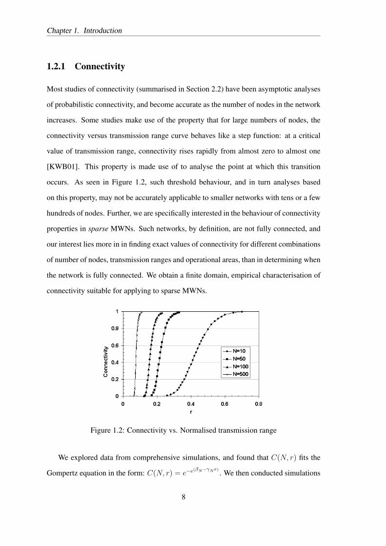
Connectivity is an important and well-studied property of wireless multi-hop networks.

Most studies of connectivity (summarised in Section 2.2) have been asymptotic analyses

of probabilistic connectivity, and are more suitable for networks with large numbers of

nodes. Some studies make use of the property that for large numbers of nodes, the

connectivity versus transmission range curve behaves like a step function: at a critical

value of transmission range, connectivity rises rapidly from almost zero to almost one

[KWB01]. This property is made use of to determine the point at which this transition

occurs.

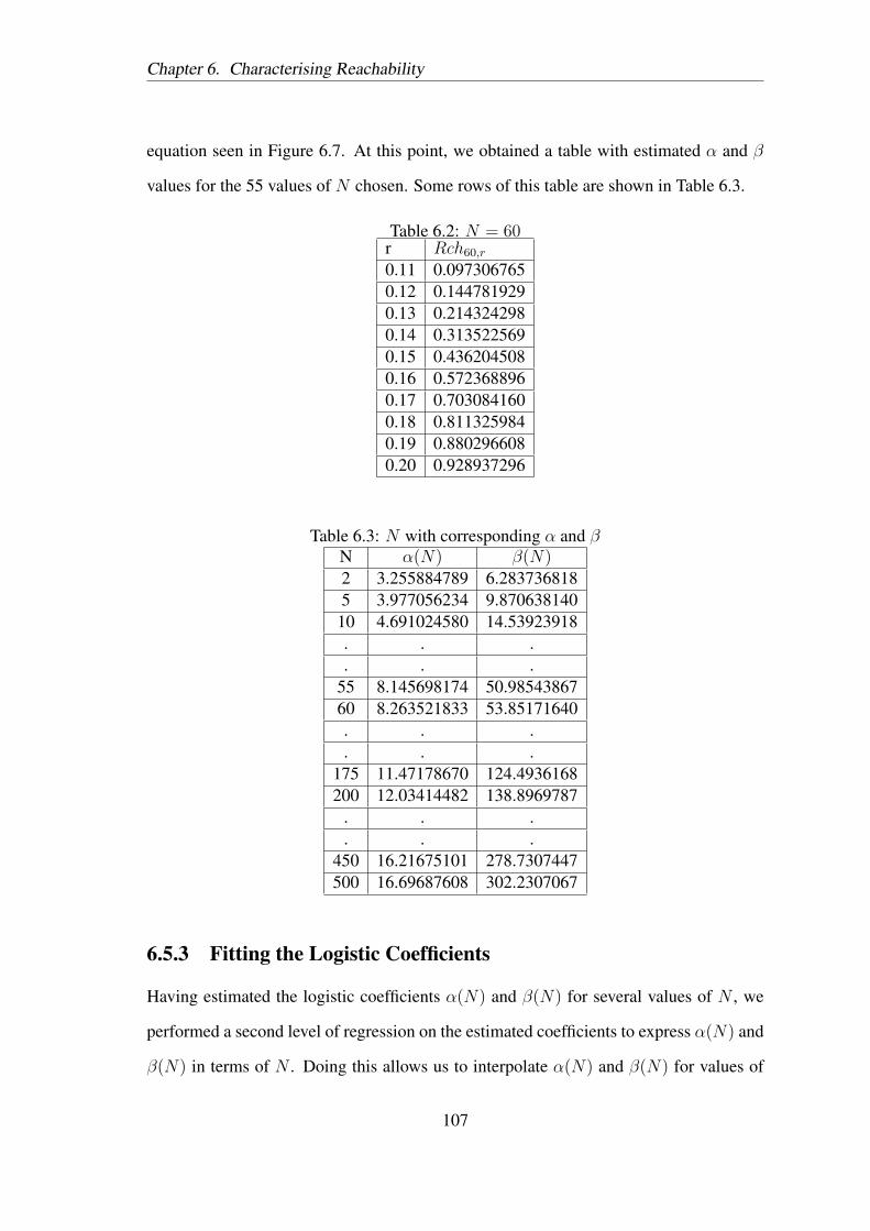
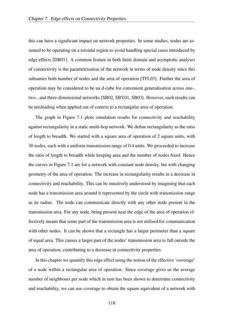
Figure 3.1 illustrates the growth curves for connectivity against normalised trans-

mission range for increasing numbers of nodes. The curve begins to resemble a step

function only beyond N = 100. This threshold behaviour, and in turn analyses based on

this property, may not be accurately applicable to smaller networks with tens or even a

few hundreds of nodes. Further, we are specifically interested in the behaviour of con-

nectivity properties in sparse multi-hop wireless networks. Such networks, by definition,

are not fully connected, and our interest lies more in finding exact values of connectiv-

37

Chapter 3. Characterising Connectivity

ity for different combinations of number of nodes, transmission ranges and operational

areas, than in determining when the network is fully connected.

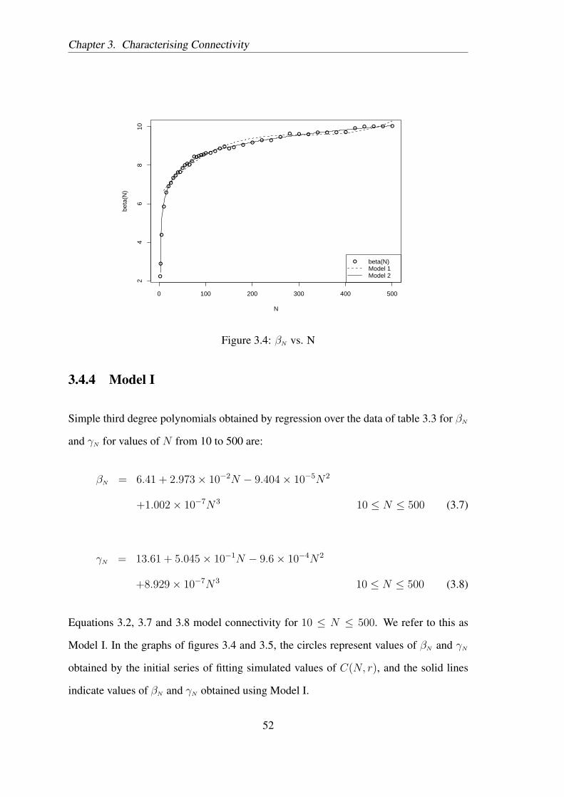
Figure 3.1: Connectivity vs. Normalised transmission range

In this chapter we present empirical regression based equations for connectivity of

a two-dimensional, static wireless multi-hop network (sections 3.4.4 and 3.4.5). The

regression is on simulated data, and we present the required background on regression

(Section 3.2) and details about planning the simulations (Section 3.4). The obtained

closed form expressions are in terms of number of nodes and transmission range of nodes,

and are valid for nodes ranging from 3 to 500 in number that are distributed uniformly at

random in a square area of operation. We also compare our results with existing related

work (Section 3.6).

3.1.1 Network model and assumptions

We make the following network assumptions commonly used in connectivity related

work (Section 2.2):

• the nodes of the network are static and uniformly distributed at random in a square

area of operation;

• all nodes have a uniform transmission range;

38


• two nodes can communicate directly if the distance separating them is not greater

than the transmission range;

In addition, we use a transmission range that is normalised to the side of the square

area either explicitly by dividing by the side of the square, or implicitly, by assuming

the square to be of unit area. The network is capable of multi-hop communication: if

a network graph is drawn with nodes as vertices, with edges connecting every pair of

nodes within transmission range of each other, two nodes can communicate if there is a

path between them of length one or greater. The network graph is said to be connected if

all the nodes are part of the same connected component.

Note that the notion of connectivity used in this work and other related work is prob-

abilistic in nature. This is because a network defined by its parameters such as number

of nodes, transmission range and side of the square area of operation, can have many

different instances depending on the exact positions of the nodes. The connectivity for

each of these network instances is a binary value—that is, an instance is either connected

or not. But given a large number of network instances, the fraction that are connected

represents the probability that a random instance of the network will also be connected.

This probability represents the connectivity of the network.

There is some overlap in the use of the term ‘connectivity’ in the area of topology

control in multi-hop wireless networks. The k-connectivity of a network graph is a mea-

sure of its fault tolerance capability. A graph is said to be k-connected if there exists a

path between all remaining pairs of nodes when k − 1 nodes are removed. Or equiv-

alently, if there exist at least k distinct paths between any pair of nodes. Expressed in

these terms, the notion of connectivity used in our work is as follows: the connectivity of

a network is the probability that the network is 1-connected. Examples of related work

that also use this notion are [TFL03], [DM02], and [Kos04].

39


3.2 Background: Regression analysis

A regression model allows us to estimate or predict a random variable as a function of one

of more other variables. The estimated variable is called the response variable, and the

variables used to predict the response are called predictor variables. In this chapter, we

use regression to model connectivity (C(N, r)) as a function of the number of nodes in

the network (N ), and the nodes’ transmission range normalised by the side of the square

area of operation (r). Although the techniques and models used are standard practice, we

briefly explain them here for completeness.

3.2.1 Linear Regression

In simple linear regression, the response variable is modelled as a linear function of a

single predictor variable. Of the many lines that potentially fit the points given by the

instances of the predictor variable, one needs to be chosen. One criterion to define the

best linear model is to pick the model that minimises the sum of squares of the errors.

This is known as least-squares regression [Jai91]. Let the linear model be of the form

y = b0 + b1x

where y is the predicted response when the predictor variable is x. The parameters b0 and

b1 are fixed regression parameters to be determined from the data. Given n observation

pairs (x1, y1), ..., (xn, yn), the estimated response yi is given by yi = b0 + b1xi, with the

error in the model given by ei = yi − yi. Then, the best linear model is given by the

regression parameter values that minimise the sum of squared errors,

n∑i=1

e2i =n∑i=1

(yi − b0 − b1xi)2

40


subject to the constraint that the mean error is zero,

n∑i=1

ei =n∑i=1

(yi − b0 − b1xi) = 0

It can be shown that this constrained minimisation problem is equivalent to minimising

the variance of errors [Jai91].

The model parameters are estimated as

b1 =Σxy − nxyΣx2 − n(x)2

, b0 = y − b1x

where

x =1

n

n∑i=1

xi y =1

n

n∑i=1

yi

Σxy =n∑i=1

xiyi Σx2 =n∑i=1

x2i

The above equations are substantially from [Jai91] where they are also derived. In our

work, we used the R software [Tea05] for performing least-squares linear regression.

3.2.2 Goodness of fit

There are several methods to determine how closely the obtained linear model explains

the response points used to construct the model.

R2 metric

The total sum of squares (SST) is given by SST =∑n

i=1(yi−y)2, and the sum of squared

errors (SSE) is given by SSE =∑n

i=1(yi − yi)2. SST is a measure of y’s variability and

is called the variation of y. The difference between SST and SSE is the sum of squares

41


explained by the regression. The fraction of variation that is explained determines the

goodness of the regression and is called the coefficient of determination, or R2.

R2 =SST − SSE

SST

An R2 value close to one indicates a good fit between the model and the data used to

obtain it.

Visual tests

Several visual indicators can be used to evaluate the goodness of fit offered by a linear

regression model. Some of these are:

- a linear relationship in the scatter plot of y versus x values;

- no discernible trends in the scatter plot of residual errors versus predicted response;

and

- an approximately linear plot of normal quantile versus residual quantile.

Cook’s distance for the ith observation is based on the differences between the predicted

responses from the model constructed from all of the data and the predicted responses

from the model constructed by setting the ith observation aside, and is an indicator of

that point’s contribution to the regression model. A point with a Cook’s distance greater

than one may need to be investigated.

A Scale-Location plot plots the square root of residuals against the predicted re-

sponses. Taking the square root of the residuals is intended to diminish skewness.

42


3.2.3 Curvilinear Regression

When the relationship between the response and predictor variables are non-linear, we

may be able to transform the non-linear function into a linear one. Such a regression

is called curvilinear regression [Jai91]. The goodness of fit tests indicated for linear

regression are also applicable here. The obtained linear function can be transformed to

its original non-linear form by applying the inverse transformation.

3.3 Characterisation of Connectivity

Our model is in terms of the number of nodes, N , their uniform transmission range,

R, and the side of the square area of operation, l. Since networks are scale models of

each other when their R/l ratios are equal, we can subsume R and l into a normalised

transmission range, r = R/l. We characterise connectivity as a function of N and r, and

denote it as C(N, r).

We explored simulated data for C(N, r) versus r for several values of N between 3

and 500 to find a suitable regression model. The plots showed a sigmoidal growth curve,

asymmetric about its point of inflexion. We used [Rat93], which provides a classifica-

tion of non-linear regression models based on shape and behaviour of the curve, number

of regression parameters, and estimation behaviour of the function, to identify potential

regression functions. We then fit our simulated data with these functions and compared

statistics and results of visual tests for goodness of fit. These comparisons were per-

formed in the Simfit regression modelling tool [Bar], which allows iterative fitting with

different functions, and provides detailed comparisons between the quality of fits.

The simplest model to fit C(N, r) accurately was a three-parameter model called the

43


Gompertz model [Rat93]. It is written in its general form as:

y = αe−e(β−γx)

(3.1)

where α is the upper asymptote and βγ

is the point of inflexion, that is, the value of x at

which the rate of growth of the curve is maximum. Since we are modelling the growth of

C(N, r) as r increases, and since C(N, r) has an upper asymptote of 1, we can rewrite

Equation 3.1 as:

C(N, r) = e−e(βN−γNr) (3.2)

requiring us to estimate only two parameters, βN and γN , for any given value of N .

In order to characterise C(N, r) we:

• conducted simulations to obtain data representing the growth of C(N, r) from 0 to

1 as r increased, while keeping N fixed;

• used Equation 3.2 as a regression function for simulated data, and obtained the

coefficients β and γ for the corresponding value of N, allowing us to characterise

connectivity as a function of r for one value of N;

• repeated the above two steps for values of N ranging from 3 to 500, and performed

a second level of regression on the estimated values of βN and γN .

This gave us a set of equations that allows us to obtain C(N, r) for values of N ranging

from 3 to 500. While our characterisation itself was for a static network, it can be applied

to mobile networks where nodes move such that their uniform distribution is preserved.

44


3.4 Details about simulation and curve fitting

We performed simulations using Simran, a simulator we have built for topology related

simulations. Details about Simran can be found in Chapter 8. Regression analysis was

performed using the R environment [Tea05, Ver02] and Simfit [Bar].

3.4.1 How many simulations?

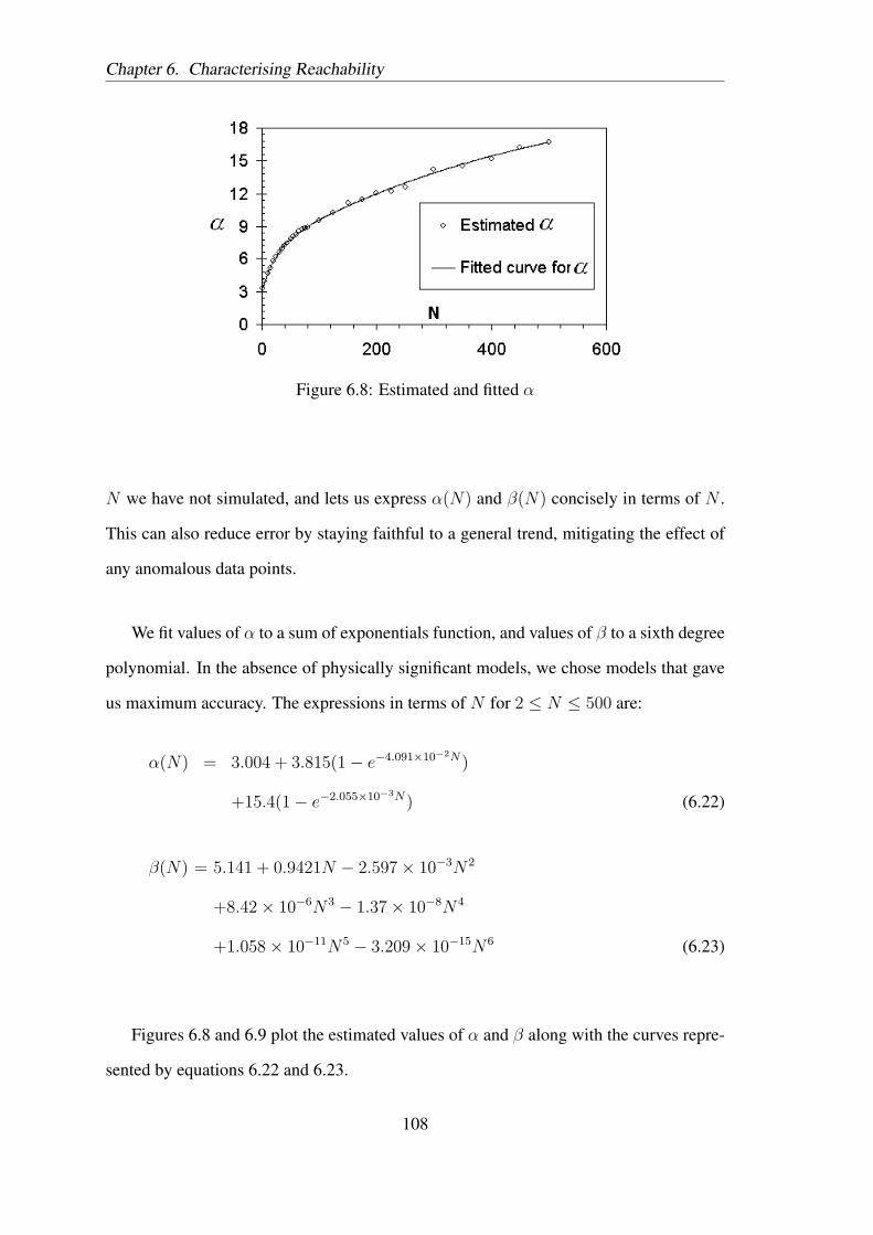
Figure 3.2: Standard Deviation vs. Connectivity for 90 nodes

A single static arrangement of nodes is either completely connected or not. We es-

timate C(N, r) by determining the fraction of network instances with N nodes and r

normalised transmission range that are connected. This fraction calculated over many

network instances is an estimate of the probability that a network with N nodes and nor-

malised transmission range of r will be connected. We conduct n runs using different

node arrangements coming from a uniformly random distribution. The result of each run

is a 1 if the network is connected, and a 0 if it is not. The mean of these results gives our

estimate of C(N, r). For the purpose of discussion in this section, we call this the sam-

ple mean. The actual value C(N, r) is called the population mean. We now determine

the value of n required to obtain an estimate of C(N, r) accurate to within 1% with a

confidence of 95%.

45


When the sample mean is x, using the central limit theorem, a 100(1 − α)% confi-

dence interval for the population mean is given by:

(x− z1−α

2

s√n, x+ z1−α

2

s√n

)

where x is the sample mean, s is the sample standard deviation, n is the sample size, and

z1−α2

is the (1− α2)-quantile of a unit normal variate [Jai91]. Substituting for z0.025 from

the unit normal distribution table, we can say with 95% confidence that the population

mean lies within:

x± 1.96s√n

(3.3)

Given the outcomes of the n runs, we can determine s, the standard deviation of the

sample as [Jai91]:

s =

√√√√ 1

n− 1

n∑i=1

(xi − x)2 (3.4)

Alternatively, a computational formula that allows us to compute s in a single pass is

given by [Mos86]:

s =

√√√√ 1

n− 1

[ n∑i=1

x2i −

1

n

( n∑i=1

xi

)2](3.5)

For us to be able to use Equation 3.3, we need to compute the value of s. This value

can change depending on the values of N and r. Therefore, we shall compute an upper

bound on the value of s that can occur, and use it to find a suitable n. If n network

instances are simulated, let the fraction that are connected be p. Since the outcome

of each simulation is either 0 or 1, the mean value of n simulations is also p. Also,

46


q = (1− p). Substituting in Equation 3.4 we get:

s =

√√√√ 1

n− 1

n∑i=1

(xi − p)2

s =

√1

n− 1[np(1− p)2 + nq(−p)2]

s =

√1

n− 1[npq2 + nqp2]

s =

√n

n− 1[pq(q + p)]

s =

√n

n− 1pq

Since nn−1

is very nearly equal to 1, especially when n becomes large, we can write:

s ≈ √pq

Note that this can also be derived differently1. Since p + q = 1, pq takes its maximum

value when p = q = 0.5. This gives us a corresponding maximum s value of 0.5. (Figure

3.2 shows the variation of standard deviation with connectivity for 90 nodes. Values

of standard deviation for the plot were obtained by using Equation 3.5 on the results

of 10000 simulations.) Intuitively, this corresponds to the cases when N and r values

are such that C(N, r) is 0.5. When C(N, r) is close to 0 or 1, most observations have

the same value, that is, either 0 or 1, and hence the variability is low. However, when

C(N, r) is close to 0.5, every sample point, which again is either 0 or 1, is away from

the mean by around 0.5. Using this maximum value of s in Equation 3.3 gives us a value

of n that ensures that our estimate of C(N, r) is within 1% of the actual value with 95%

1Since the outcome associated with a network instance is binary (connected or not-connected), we canalso obtain the same result by representing the outcome of each run as a Bernoulli random variable. Whenthe probability of occurrence and non-occurrence are p and q respectively, the variance of a Bernoullirandom variable is is given by pq [Tri01], and therefore, its standard deviation by

√pq.

47


confidence. We do this by ensuring the following inequality:

1.96× 0.5√n

≤ 0.01

0.98√n≤ 0.01

n > (0.98

0.01)2

n > 9604

For our simulations we choose n = 10000.

3.4.2 Simulations

We conducted simulations for 44 values of N between 2 and 500. For each value of N,

we conducted simulations for different values of r. These were chosen such that sample

values of C(N, r) were obtained at enough points in the interval [0,1] to permit accurate

regression modelling. Each (N, r) pair was simulated over 10000 static arrangements

of nodes distributed uniformly at random. At the end of these simulations, we obtained

tables for the growth of C(N, r) with r for each of the 44 chosen values of N. For illus-

tration, tables corresponding to N = 30 and N = 300 are presented in tables 3.1 and

3.2.

3.4.3 Regression

Since we have data for the growth of C(N, r) versus r, we use regression analysis to

obtain estimates for βN and γN of Equation 3.2 for the 44 values of N simulated. In the

next phase, we perform regression on the values of βN and γN to obtain an expressions

for βN and γN in terms of N.

48


r C(30, r)0.21 0.019

0.225 0.06770.235 0.12550.245 0.20810.255 0.30540.265 0.40580.275 0.50550.285 0.59990.295 0.67870.31 0.77780.34 0.89770.36 0.94210.4 0.9806

Table 3.1: Simulated Data for N=30

r C(300, r)0.08 0.01610.084 0.06490.086 0.11250.088 0.17680.09 0.2450.092 0.32340.094 0.40450.096 0.47920.098 0.55160.1 0.618

0.104 0.7280.108 0.81210.118 0.92620.13 0.9753

Table 3.2: Simulated Data for N=300

Equation 3.2 can be written as:

ln(−ln(C(N, r))) = βN − γNr

FN = βN − γNr (3.6)

which is linear in r. Using this form, we perform linear regression with FN as the predic-

tor variable and r as the response variable for each of the 44 chosen values of N to obtain

Table 3.3. The last column of the table shows the R2 goodness of fit metric defined in

section 3.2.2. The values of R2 close to 1 indicate a strong linear relationship in the data.

For illustration, we take a closer look at the fit for N = 30. Figure 3.3(a) plots the

simulated points representing the predictor variable, F30, and the corresponding fitted

straight line. This line is given by

F30 = 7.3345− 28.1334r

after substituting values for β30 and γ30 from Table 3.3 into Equation 3.6.

Figure 3.3(b) shows summary statistics for the linear regression for N = 30. In the

49


●

●

●

●

●

●

●

●

●

●

●

●

●

0.25 0.30 0.35 0.40

−4

−3

−2

−1

01

r

F

(a) Linear fit

−4 −3 −2 −1 0 1

−0.

040.

00

Fitted values

Res

idua

ls

●

●

●●●

●●

●●

●●

●

●

Residuals vs Fitted

1

12

7

●

●

● ● ●

● ●

●●

●●

●

●

−1.5 −0.5 0.5 1.5

−2

−1

01

Theoretical Quantiles

Sta

ndar

dize

d re

sidu

als

Normal Q−Q plot

1

12

7

−4 −3 −2 −1 0 1

0.0

0.5

1.0

1.5

Fitted valuesS

tand

ardi

zed

resi

dual

s ●

●

●●●

●●

●

●

●●

●

●

Scale−Location plot1

12

7

2 4 6 8 10 12

0.0

0.4

0.8

Obs. number

Coo

k's

dist

ance

Cook's distance plot1

1312

(b) Fitting statistics

Figure 3.3: Linear fit for F vs. r for N = 30

upper left is a scatter plot of residuals versus fitted values. Points in the centre seem to

be above the zero line, but this is not a very discernible pattern, and is not visible in the

Scale-Location plot which plots the square roots of the residuals to reduce skew. The

normal quantile versus residual quantile plot displays slight evidence of non-linearity,

and the Cook’s distance plot indicates that the first point of the data has the largest influ-

ence on the regression model. These factors do not allow us to conclude that the linearity

of the fit is perfect. However, the fact that the residual values are small indicates that

the model is acceptable. (Similar analyses of linear fitting case studies can be found in

[Jai91].) As can be seen from figures 3.4 and 3.5, βN and γN grow with increase in N .

We can use the values in table 3.3 to generate regression models for βN and γN over the

N values in the range of interest.

50


Table 3.3: N, βN , γN and R2

N βN γN R2

2 2.2364 5.4987 0.94413 2.8925 6.2940 0.96855 4.3857 9.5573 0.970310 5.8514 14.9225 0.988315 6.5842 19.2227 0.994720 6.9059 22.4932 0.997825 7.0835 25.1986 0.999630 7.3345 28.1334 0.999835 7.4651 30.5190 0.999940 7.6277 33.0017 0.999945 7.6442 34.8398 0.999450 7.8521 37.4772 0.999455 7.9990 39.8436 0.999460 8.0788 41.8016 0.999265 8.0272 43.1168 0.998670 8.2140 45.4827 0.999175 8.4454 48.1711 0.999580 8.4236 49.5153 0.999485 8.4786 51.2058 0.999290 8.5279 52.8564 0.999395 8.5527 54.3398 0.9993100 8.6231 56.0814 0.9990110 8.6360 56.0814 0.9991120 8.7298 61.6422 9989130 8.8656 64.8565 0.9994140 8.9744 67.9537 0.9992150 8.8631 69.2890 0.9990160 8.9281 71.7544 0.9984180 9.0528 76.9010 0.9988200 9.1758 81.7448 0.9984220 9.2947 86.4599 0.9982240 9.2927 89.8950 0.9983260 9.4660 94.9817 0.9990280 9.6379 100.2136 0.9994300 9.6134 103.0714 0.9991320 9.6022 105.9842 0.9992340 9.6956 110.0233 0.9990360 9.6956 112.9008 0.9989380 9.7008 115.7980 0.9987400 9.7120 118.5848 0.9984420 9.9182 123.6922 0.9992440 10.0026 127.6732 0.9993460 10.0126 130.2024 0.9991480 10.0109 132.6134 0.9989500 10.0307 135.4894 0.9985

51


●

●

●

●

●

●●

●●

●●●

●●●●

●●●●●● ● ●●

●● ●

●●

● ●●

● ● ● ● ● ● ●● ● ● ● ●

0 100 200 300 400 500

24

68

10

N

beta

(N)

● beta(N)Model 1Model 2

Figure 3.4: βN vs. N

3.4.4 Model I

Simple third degree polynomials obtained by regression over the data of table 3.3 for βN

and γN for values of N from 10 to 500 are:

βN = 6.41 + 2.973× 10−2N − 9.404× 10−5N2

+1.002× 10−7N3 10 ≤ N ≤ 500 (3.7)

γN = 13.61 + 5.045× 10−1N − 9.6× 10−4N2

+8.929× 10−7N3 10 ≤ N ≤ 500 (3.8)

Equations 3.2, 3.7 and 3.8 model connectivity for 10 ≤ N ≤ 500. We refer to this as

Model I. In the graphs of figures 3.4 and 3.5, the circles represent values of βN and γN

obtained by the initial series of fitting simulated values of C(N, r), and the solid lines

indicate values of βN and γN obtained using Model I.

52


●●●

●

●●

●●

●●

●●

●●●

●●●

●●●●

●●

●● ●

●

●

●

●●

●

●●

●●

●●

●

●●

●●

●

0 100 200 300 400 500

2040

6080

100

120

140

N

gam

ma(

N)

● gamma(N)Model 1Model 2

Figure 3.5: γN vs. N

3.4.5 Model II

Model I is only valid in the range 10 ≤ N ≤ 500. Attempting to extend the model on

the lower side results in a loss of accuracy. We can obtain more accurate and general

expressions for βN and γN by performing piece-wise fitting of the data in Table 3.3. In

Figure 3.4, note that the curve has a knee at around N = 130. Using separate equations

to mode the curves for N < 130, and for N ≥ 130 allows the model to be more accurate.

Following a process similar to that described in section 3.3, we chose two-parameter

curves of the form y = log(a + bx) to fit βN [Rat93]. This form is easily reduced to a

straight-line form suitable for linear regression:

eβN = aN + b

Figures 3.6(a) and 3.7(a) give a visual indication of goodness of fit. Other statistics for

the two fits are in figures 3.6(b) and 3.7(b).

We also split the curve for γN , using a sum of exponentials for the segment below

53


N = 130 and a quadratic for 130 ≤ N ≤ 500). Note that we choose N = 3 as our

starting point since exact expressions for connectivity are available for N = 2.

The model obtained is as follows:

βN =

log(55.74N − 155.72) 3 ≤ N < 130

log(44.42N + 953.59) 130 ≤ N ≤ 500(3.9)

γN =

102.13− 11.26e−0.1678N

−90.87e−6.801×10−3N 3 ≤ N < 130

30.57 + 0.285N

−1.511× 10−4N2 130 ≤ N ≤ 500

(3.10)

Equation 3.2 with equations 3.9 and 3.10 form Model II for C(N, r). In the graphs

of figures 3.4 and 3.5, the circles represent values of βN and γN obtained by the initial

series of fitting simulated values of CN,r, and the solid lines indicate values of βN and γN

obtained using Model II.

●●

●

●

●●

●●

● ●

●

●

●●

●

●●

●

●●

● ●

●

●

0 20 40 60 80 100 120

010

0020

0030

0040

0050

0060

0070

00

N

exp(

beta

(N))

(a) Linear fit

0 2000 4000 6000

−40

020

0

Fitted values

Res

idua

ls

●●●●●

●●●●

●

●●●

●

●

●

●●●●

●

● ●

●

Residuals vs Fitted16

14 23

●●●●●

●●

● ●

●

●●●

●

●

●

●●●

●●

●●

●

−2 −1 0 1 2

−2

02


Sta

ndar

dize

d re

sidu

als

Normal Q−Q plot16

14 23

0 2000 4000 6000

0.0

1.0

Fitted values

Sta

ndar

dize

d re

sidu

als

●

●●●●●●

●●

●

●●●

●

●

●

●●●

●

●

● ●

●


14 23

5 10 15 20

0.00

0.15

0.30

Obs. number

Coo

k's

dist

ance


1622


Figure 3.6: eβN vs. N, 3 ≤ N < 130

54


●

●

●●

●

●

● ●

●

●● ●

● ● ● ●

●

●● ●

●

200 300 400 500

1000

015

000

2000

0

N

exp(

beta

(N))

(a) Linear fit

10000 15000 20000

−20

000

2000

Fitted values

Res

idua

ls

●

●

●● ●●

●

●

●

●

●

●

●

●

●

●

●

●

●

●

●

Residuals vs Fitted

16

1018

●

●

●● ●●

●

●

●

●

●

●

●

●

●

●

●

●

●

●

●

−2 −1 0 1 2

−2

−1

01

2


Sta

ndar

dize

d re

sidu

als

Normal Q−Q plot

16

1018

10000 15000 20000

0.0

0.5

1.0

1.5

Fitted values

Sta

ndar

dize

d re

sidu

als

●

●

●●●

● ●

●

●

●

●

●

●

●

●

●

●

●

●

●

●


1018

5 10 15 20

0.00

0.10

0.20

Obs. number

Coo

k's

dist

ance


18

10


Figure 3.7: eβN vs. N, 130 ≤ N ≤ 500

3.5 Validation

For validation, and to estimate the error present in models I and II, we compared the

values of connectivity generated by the models with that obtained by running simulations

for 236 pairs of N and r values. We chose 59 values of N that did not contribute towards

the model, and for each of those values of N , we chose four values of r such that the

resulting value of C(N, r) would lie between 0.05 and 0.95. This choice of r is required

because for a given value of N , there is only a narrow range of r values that will yield

values of C(N, r) between 0 and 1. If r were to be chosen randomly, the resulting

C(N, r) value would most often be very close to 0 or 1, and would not test the model.

We conducted 10000 simulations in Simran for each of the chosen (N, r) pairs, and

compared the resulting connectivity with that obtained from Model I given by equations

3.2, 3.7 and 3.8. For values of N below 30, we found that the model had a mean absolute

error of 0.0691, with the maximum error seen being 0.1756. The model is more accurate

for values of N above 30 with a mean absolute error of 0.0116, with the maximum error

seen being 0.044. Model II proved to be much more accurate than Model I. The mean

absolute error over the 236 values after ignoring signs was 0.0089. The maximum error

55


observed across all instances was 0.0418.

3.6 Comparison with other work

We compare the models we have obtained with the model obtained in [TFL03] given

by equations 2.1, 2.2, and 2.3, which we refer to as Model III. (More details about this

model can be found in Section 2.2.3.) This model is less generic, being for values of

connectivity between 0.5 and 1, and for networks with 3 to 125 nodes. The authors of

[TFL03] validate their model (Model III) by comparing values of connectivity obtained

by simulation and Model III for 5 sets of network parameters. Table 3.4 shows a com-

parison between the values of connectivity obtained by simulation, by using Model III,

and by using our models, Model I and Model II. The Table 3.4 is from [TFL03] after

converting parameters to our notation for consistency of presentation. Model I yields

values closer to the simulated values than Model III in four out of five instances. With

Model II, all the five instances show values of connectivity closer to the simulated values

than with Model III.

The regression model for connectivity presented in [TFL03], and summarised in Sec-

tion 2.2.3 is applicable for P ∈ [0.5, 0.99] and n ∈ [3, 125]. The model we present in this

chapter 3 is more general, being applicable for P ∈ [0.05, 0.95] and n ∈ [3, 500]. This

applicability for values of connectivity less than 0.5 covers the sparse region of operation

more thoroughly.

56


Table 3.4: Comparison of Models

N r C(N, r) (Simulated) C(N, r) (Model III) C(N, r) (Model I) C(N, r) (Model II)40 0.3 0.909 0.8974 0.8988 0.898020 0.4 0.8852 0.8589 0.9100 0.885136 0.26 0.5697 0.5532 0.5729 0.554581 0.2 0.8115 0.8390 0.7956 0.812160 0.21 0.6195 0.6364 0.5941 0.6059

57


58

Chapter 4

Reachability

In Chapter 3 we characterised connectivity in the finite domain for sparse, static, two-

dimensional networks1. This was to enable the making of fine-grained tradeoffs between

network parameters while designing sparse MWNs. However we claim that using con-

nectivity as a metric for topology design in sparse networks can prove inadequate because

i) connectivity is not indicative of the actual extent to which the network can support

communication; and ii) it is unresponsive to fine changes in network parameters. For

example, it is possible that a sparse network which allows a significant number of nodes

to communicate has a connectivity close to zero. Further, an increase in some network

parameter such as number of nodes, or transmission range, may increase the ability of

nodes to communicate, but it may not be reflected by a corresponding increase in con-

nectivity. We believe that a property of the network graph better suited for use with

sparse networks is the fraction of node pairs that are connected. We call this property

reachability. Both connectivity and reachability are different connectivity properties of a

network graph.

Figure 4.1 is obtained from simulations, and plots the growth of reachability and

connectivity as the uniform transmission range of nodes, R, increases for 60 static nodes

1Recall that we defined a sparse MWN in terms of connectivity as a network with a connectivity valueless than 0.95.

59

Chapter 4. Reachability

distributed uniformly at random in a 2000m × 2000m area. In this case, when reachabil-

ity is 0.4, meaning 40% of node pairs are connected, connectivity is still at zero. Further,

using only connectivity here would lead us to believe that increasing R from 50m to any

value less than 320m would have no effect on the extent of communication supported by

the network. This example is taken from a case study presented in Chapter 5. The case

study also goes on to show that connectivity is an even more misleading indicator in the

presence of mobility and asynchronous communication. In the rest of this chapter, we

define reachability and discuss its properties and applications.

Figure 4.1: Increasing R, no mobility

4.1 Reachability

The reachability of a static network is defined as the fraction of connected node pairs in

the network. As defined in Equation 1.1, we can calculate reachability for a network of

N nodes as2:


N2

) (4.1)

A pair of nodes is considered connected if there is a path of length one or greater between

2We assume that communication links between nodes are symmetric.

60


Figure 4.2: A network instance with Reachability = 0.378

them. Figure 4.2 shows one instance of a network with 10 nodes. We count the number

of node pairs that can reach each other, that is, nodes that are connected either directly or

through other nodes, as 17. Substituting N = 10 in the denominator of Equation 4.1, we

obtain the reachability for this network instance as 17/45 or 0.378.

It is possible that a different network instance with 10 nodes can have a different value

of reachability. Recall that we define a network by the number of nodes, their bounding

area, and the transmission ranges of the node. For the same network, there can exist

many different network instances with different corresponding values of reachability.

We define the network’s reachability as the mean reachability across several instances.

As we will show later in this chapter, this value is significant because it represents the

probability that that there exists a path between an arbitrary pair of nodes in the network.

4.2 Reachability in mobile and asynchronous MWNs

4.2.1 Reachability for mobile MWNs

When nodes are mobile, the fraction of connected node pairs varies with time depending

on the pattern of node movements. However a single value can be obtained for any time

instant. We define the reachability of a mobile network to be the average of instantaneous

reachability values measured at frequent intervals during the operation of the network.

Note that the definition of reachability is independent of the distribution of nodes.

That is, given any network graph, we can calculate the corresponding reachability. How-

61


ever, in most cases of practical interest, we only have a distribution of nodes. In such

cases, using reachability for topology design is much more meaningful when nodes are

mobile: if a network is designed for a certain value of reachability, the measured reacha-

bility of a mobile network converges with time to the reachability value used for topology

design. This is not the case in a static network because there is only a single instance that

will be deployed, and its reachability value may differ from the value used for design.

4.2.2 Reachability for asynchronous MWNs

In asynchronous networks (described in Section 2.3.1), nodes can buffer packets when

a path to the destination is unavailable, and forward it at a later time after mobility has

brought about some change in the network graph. We define the reachability of an asyn-

chronous MWN in the same way as for mobile MWNs: it is the average of instantaneous

reachability values measured at frequent intervals.

Instantaneous reachability at any point of time in the operation of the network is

measured as the fraction of connected node pairs at that instant. However, the notion

of ‘connected node pair’ needs revisiting in the context of mobile and asynchronous

networks.

4.2.3 When is a node pair connected?

In the static case we have considered a node pair as connected if they there exists a multi-

hop path between them in the network graph. This notion may need to be qualified by

several conditions when the network is mobile or has the capability to form asynchronous

paths.

When nodes are mobile, there could be a minimum time for which a path would have

to exist for it to be useful for communication. Therefore a node pair that is connected

for a time less than some pre-defined threshold may be considered unconnected while

62


calculating instantaneous reachability. For the rest of this thesis, we make the assumption

that this threshold is negligibly low, and consider a node pair connected at an instant if a

path between them exists at that instant.

The case of asynchronous networks involves mobility with buffers being present at

the nodes. A node could then form a disjoint path to another node in which a path

between the two nodes did not exist at any single point in time. In such cases, we count

all node pairs with such a disjoint path as connected. In later chapters, we add a network

parameter to represent the extent of such asynchronous communication possible: this

takes the form of the maximum time for which a packet can be buffered in the network.

A simple example is when only source nodes buffer packets: if we are studying a network

where source nodes without a route to the destination buffer packets for 30 seconds, the

number of connected node pairs at a time instant would include a particular pair of nodes

if there existed a path between them at that instant, or within 30 seconds from that instant.

4.3 Properties of Reachability

We state and prove the following claims:

1. The reachability of a network lies in the interval [0, 1].

2. Reachability of a sparse network is not less than the connectivity of the same net-

work.

3. Reachability represents the probability that there exists a path between a randomly

chosen pair of nodes in an MWN.

4. Reachability of a network represents the long term maximal packet delivery ratio

achievable between random source-destination pairs in the network.

Claim 1: Reachability of a network lies in the interval [0, 1].

63


Proof: The proof follows from our definition of reachability. The lowest value that the

numerator in Equation 4.1 can take is 0. This happens when all the nodes in the network

are isolated. The largest value for the numerator is(N2

), and occurs when all node pairs

are connected.

Claim 2: Reachability of a sparse network is not less than the connectivity of the network.

Proof: Consider observations of k network instances. Let m of the k instances show a

single connected component containing all the nodes in the network. Then we determine

the connectivity of the network as mk

. The reachability of the same network is measured

by averaging the reachability obtained for each of the k network instances according to

Equation 4.1. We have the following two cases:

Case N = 2: When there are two nodes in the network, reachability is 1 for the

m instances in which the two nodes are connected, and 0 for the remaining (k − m)

instances. Therefore, for N = 2, both connectivity and reachability have the same value

of mk

.

Case N > 2: When there are more than two nodes in the network, the connectivity

continues to be mk

. In each of the m instances where the network is completely con-

nected, the corresponding reachability value is 1 by definition. Therefore, the value of

reachability for the network is at least mk

. In addition, reachability values for the m − k

unconnected instances lie in the interval [0, 1) as already shown3. Therefore, the mean

reachability for the network must lie in the interval [mk, 1].

Claim 3: Reachability represents the probability that a randomly chosen pair of nodes

in the network is connected.

Proof: Let k instances of a network be observed. Let the number of connected node pairs

in the ith instance be denoted by ci. We then calculate the probability that a randomly

3The closed interval in [0, 1) is due to the knowledge that the (k −m) instances considered here arenot fully connected, and cannot therefore have a reachability of 1.

64


chosen pair of nodes in the network is connected as the sum of the connected node pairs

in the observed instances divided by the total number of observed node pairs:

c1 + c2 + . . .+ ck

k(N2

) (4.2)

Reachability for the same network is measured as the averaged reachability values of

the k instances, which can be written as:

1

k

(c1(N2

) +c2(N2

) + . . .+ck(N2

)) (4.3)

Expressions 4.2 and 4.3 are equivalent.

Claim 4: Reachability of a network represents the long term maximal packet delivery

ratio achievable between random source-destination pairs in the network.

Proof: Given a network instance, the most thorough measurement of Packet Delivery

Ratio (PDR) would be achieved by sending packets between all pairs of nodes, and mea-

suring the fraction of packets received. Assuming no packets are dropped due to radio

interference or routing inefficiencies, the only packets that will not reach their intended

destinations are those without a path between source and destination. With N nodes in

the network, and with p packets sent between each node pair, a total of p ×(N2

)packets

will be sent. If c is the number of node pairs with a route p × c packets are delivered.

Then, for this instance:

PDR =p× cp×

(N2

) =c(N2

)The right hand side is the reachability for this network instance by definition.

65


4.4 Applications of reachability

The primary application of reachability is in topology design of sparse MWNs. In this

section we present only a brief overview of this application and defer more detailed

discussion to Chapter 5. We also discuss here the application of reachability in measuring

routing performance in MWNs.

4.4.1 Measuring routing performance

Packet Delivery Ratio (PDR) has been a popular metric for measuring the performance

of routing protocols, particularly in studies of Mobile Ad hoc Networks (MANET). In

MANETs routing is a challenging task given that links between nodes can change fre-

quently due to mobility. PDR has been used to measure the effectiveness of a routing

protocol in finding routes and delivering packets to the intended destinations in several

studies, for example [BMJ+98] and [DPR00]. PDR is usually measured by sending

bursts of traffic between different sets of node pairs in the network, and is defined as the

ratio of packets received to packets sent. The idea behind PDR is that the bursts of traffic

sample the paths between various node pairs in the network, and the fraction of packets

successfully sent across all the tested pairs is representative of the network’s ability to

carry traffic.

While PDR is a good indicator of routing ability in dense networks, it can be unindica-

tive in sparse networks. This is because PDR in a sparse network measures two properties

simultaneously:

66


1. the existence of routes between the sampled source-destination pairs; and

2. the routing protocol’s ability to exploit those routes to deliver packets.

As a result, a low value of PDR in a network may arise because of a sparse network, an

ineffective routing protocol, or both.

This ambiguity can be eliminated by using reachability to normalise the measured

value of PDR. We have shown in Claim 4 in Section 4.3, that reachability represents the

long term maximal PDR in an MWN. In other words, reachability is the PDR that would

be observed in the network if it ran a ‘perfect’ routing protocol: one that delivers every

packet to its destination, provided a route exists. Therefore, dividing observed PDR by

the network’s reachability represents the fraction of packets received between node pairs

with routes. Such a normalisation eliminates the role played by the network’s sparseness,

and provides a measure of only routing performance. Normalised Packet Delivery Ratio

(NPDR) is calculated as:

NPDR =PDR

Reachability(4.4)

Here, the value of reachability for the network in question can be obtained from simula-

tions or from models, and the value of PDR from simulated or actual measurements. In

following chapters of this thesis, we present tools and models that can be used to find the

reachability of an MWN.

4.4.2 Application: Using reachability for topology design in sparse

MWNs

Recall that we define a network using the following network parameters: number of

nodes, uniform transmission range of the nodes, and the dimensions of the area of op-

eration. Depending on the circumstances of deployment, some of these may be fixed,

67


and the designer may be able to vary the others. The intended application of the net-

work supplies more constraints: the deployment scenario may involve mobility, which

can change the connectivity properties of the network; there may be a minimum level of

communication to be supported by the network, and this may be expressed in terms of

a desired value of a connectivity property; there may be limited battery power available

per node; or there may be only a fixed number of nodes available.

These design considerations are also interdependent to a large degree. Increasing the

number of nodes is likely to increase the network’s connectivity properties, but this also

increases the cost of deployment. Trying to ensure the same level of connectivity while

using fewer nodes would require us to increase transmission range. A small increase

in transmission range could result in a large increase in the power consumption of a

node. Reachability is useful in such problems of topology design because it allows for

fine-grained evaluation of tradeoffs between network parameters. We illustrate this in

Chapter 5 with a detailed case study in which we design a sparse MWN for rural voice

communication.

68

Chapter 5

Case Study: Reachability for designing

a sparse MWN

In Chapter 4 we introduced the reachability metric as an appropriate connectivity prop-

erty for evaluating topology related design trade-offs in sparse multi-hop wireless net-

works. In this chapter, we illustrate this by using reachability to make design decisions

for a sparse MWN intended to enable communication within a rural area1 We use a

topological simulator that we have built, Simran (Chapter 8), for evaluating connectivity

properties for various configurations of network parameters. Plots of connectivity and

reachability for the scenarios of our study show that reachability is a far more indicative

measure of the extent of communication supported by a sparse MWN.

5.1 Case study scenario

5.1.1 Background

The Department of Telecommunications (DoT), India, through its Village Public Tele-

phone (VPT) scheme, aims to have at least one telephone installed in each of approx-

1This work appeared in [PI06b].

69

Chapter 5. Case Study: Reachability for designing a sparse MWN

imately six lakh (0.6 million) villages identified in the 2001 census [Dep05a]. As of

August 2005, VPTs have been deployed in 83.3% of the targeted villages [Dep05b]. The

next phase involves installing a second telephone in villages with a population over 2000.

The current focus of rural telecom initiatives is rightly to connect villages to the world

outside. At the same time, there is also a need to connect people within a village. Census

figures show that around half of all Indian villages have populations between 500 and

2000. Since these villages are predominantly agricultural, their inhabitants are spread

over fairly large areas making local communication desirable. But neither cellular nor

fixed telephony is likely to be viable in several villages for some time to come. This is

due to the service providers’ inability to recover infrastructure costs, and is borne out by

statistics which show that cellular coverage in Indian rural areas is negligible at present

[pbT04]. There are several efforts being made to bring connectivity to villages. Besides

DoT and TRAI (Telecom Regulatory Authority of India) schemes, WLL (Wireless in Lo-

cal Loop) solutions using corDECT [cor00], WiFiRe [PVI+07], and the Digital Gangetic

Plain project [BRS04] are recent initiatives to connect villages to the world outside. In

addition to these, we believe efforts are required to find ingenious ways to connect people

within a village.

5.1.2 A possible MWN solution for intra-village communication

A possible means for enabling local communication within rural areas is through deploy-

ing multi-hop wireless networks that carry packetised voice. Individuals would carry in-

expensive hand-held devices capable of encoding/decoding voice and performing multi-

hop routing. These devices would form a network that facilitates communication in two

modes: i) real-time VoIP conversations; and ii) offline voice messages. The offline voice

messaging mode would be used when the network cannot satisfy bandwidth and con-

nectivity requirements for a real-time conversation, and it can be used to communicate

70


asynchronously using store and forward mechanisms. Such a system has several advan-

tages in the rural scenario: it does not require any infrastructure deployment apart from

the hand-held devices themselves, and as a result is relatively inexpensive and quick to

deploy. This also makes it possible to use these networks as a short term arrangement

while other efforts for intra-village teleconnectivity are underway. Such a system also

does not have a single point of failure, is robust, and degrades gracefully. This is an

advantage where regular system maintenance cannot be guaranteed.

Enabling communication in remote areas is a well known application for wireless ad

hoc networks, but deploying sparse networks in constrained application scenarios is not

very well studied. Such an approach introduces an additional degree of flexibility: we

can trade deployment cost for performance depending on the application’s requirements

and the available resources. Understanding how to evaluate this trade-off is critical to

having useful deployments of sparse multi-hop wireless networks.

5.2 Design Considerations

In designing a multi-hop wireless network, some of the following parameters may be

known or given, and some will have to be decided upon by the designer: the number

of devices, capabilities and cost of each device, dimensions and topography of the de-

ployment area, usage pattern, and level of connectivity desired in the network. If the

deployment is a dense one, interference between nodes, and the resulting loss in network

capacity must also be considered.

For an application such as rural voice communication, the area of the network’s op-

eration is known. Processing power required at nodes and the bandwidth required from

radio hardware can also be determined from the application. An important considera-

tion for such an application is the overall cost of the solution. This affects the choice of

design parameters in several ways. Increasing the number of nodes is likely to increase

71


connectivity, but this also increases the cost of deployment. Trying to ensure the same

level of connectivity while using fewer nodes would require us to increase transmission

range. A small increase in transmission range can easily result in a large increase in the

power consumption of a node which would result in either a shorter life for nodes, or a

need for more expensive nodes with batteries of higher capacity. The transmission power

to be used would also depends on the physical terrain in the area of deployment: the

same transmission power would result in a longer range in a flat, field like area, and a

shorter, fluctuating range in the presence of uneven, wooded terrain. Multi-hop ad hoc

networks are also known to exhibit phase transition behaviour—a small change in trans-

mission range or the number of nodes can cause large changes in connectivity properties

[KWB01]. When nodes are capable of movement, the speed and pattern of mobility, and

their effect on network performance must also be considered.

Our aim is to choose some combination of deployment parameters that meets the

constraints of cost while providing an acceptable level of voice communication in the

village. We make the following assumptions:

• nodes can communicate if there exists a path between them, and therefore, the

extent of communication provided by the multi-hop network can be captured by a

connectivity property such as connectivity or reachability;

• the nodes have radios with power control which are to be set to a homogeneous

transmission range; and

• the node density will not be high enough for radio interference to have significant

effect.

The network parameters we consider are the number of nodes, their uniform transmission

range, and the connectivity properties of the network.

72


5.2.1 Sparse networks

An important design consideration with respect to the application is the extent of com-

munication supported by the network. Complete connectivity may be desirable, but may

not be achievable at an acceptable cost. In such cases we may be willing to tolerate a

lower degree of communication between nodes of the network. There is work that shows

that an ad hoc network willing to tolerate a small degree of sparseness can use a trans-

mission range much lesser than that required for full connectivity [SB03]. Similarly, a

sparse MWN would also need substantially fewer nodes for slightly reduced connectiv-

ity. Using fewer nodes or a smaller transmission range translates into lower deployment

costs. This ability of sparse MWNs to trade cost for connectivity makes them particularly

well-suited for economically constrained rural deployments.

For the application scenario, we use reachability as a measure of the supported com-

munication since it is: i) a more intuitive measure of the extent of communication possi-

ble between pairs of nodes; and ii) more sensitive to changes in the number of nodes or

transmission range, especially for sparse networks.

5.3 Deciding deployment parameters

Consider a village with a few hundred inhabitants that is spread over an area of 2 km

x 2 km. Quite a large portion of the village is agricultural land, contributing to the

low density of inhabitants. A number of devices capable of multi-hop packetised voice

communication are to be deployed among people in the village. We now identify design

trade-offs in this scenario through simulations.

5.3.1 Simulation Preliminaries

The simulations presented in this chapter are conducted using Simran [Per], a simu-

lator we have developed for studying topological properties of multi-hop wireless net-

73


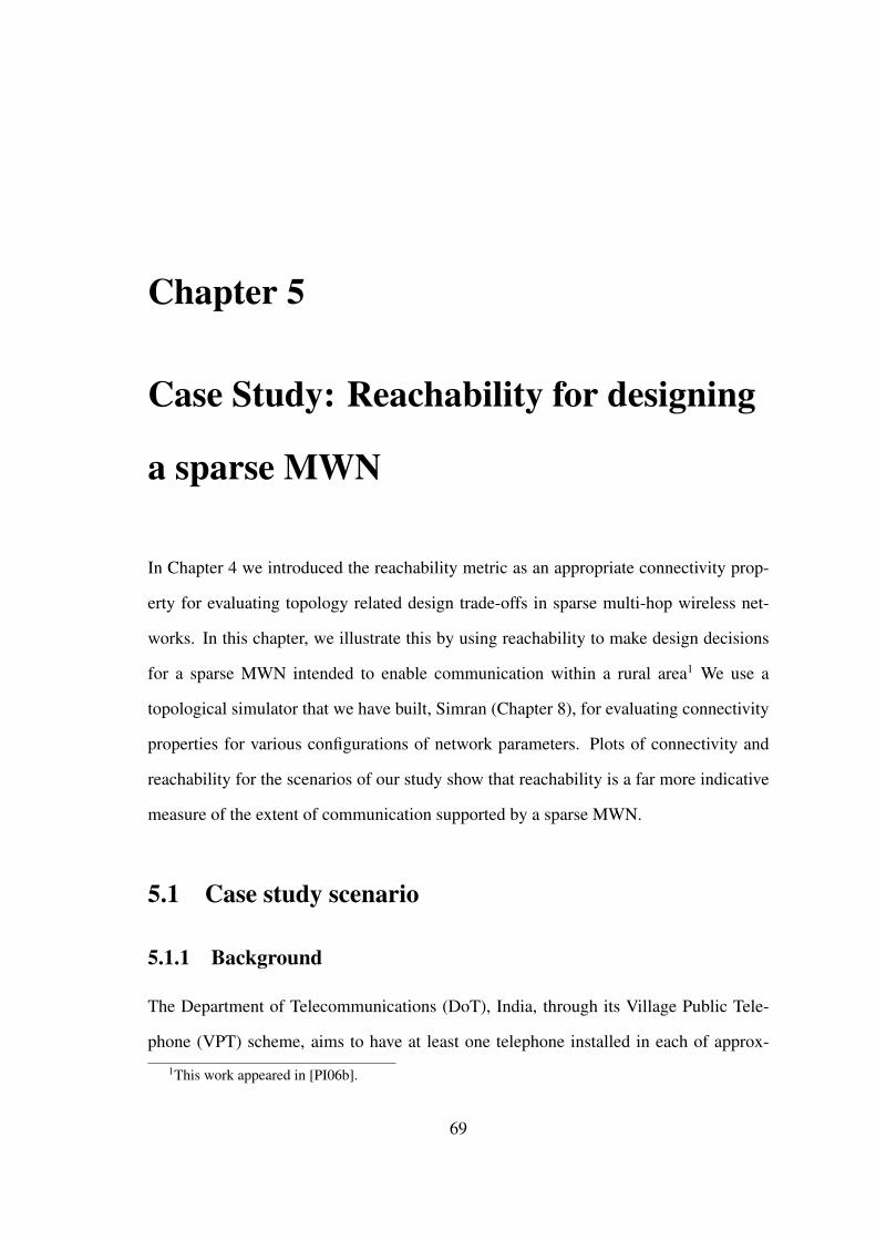
Figure 5.1: Reachability and Connectivity vs. R

works. Simran takes as input a scenario file with initial positions and movements of

nodes, and generates a trace file containing metrics of interest such as average number

of neighbours, averaged shortest path lengths over all pairs of nodes, reachability, con-

nectivity, and number and size of connected components. Simran is also supported by a

number of smaller programs for generating scenario files, managing simulations and for

analysing results. Simran also supports topological simulation of networks with asyn-

chronous communication. More details about the simulator can be found in Chapter 8.

Initially, in sections 5.3.2, 5.3.3, and 5.3.4, we assume that mobility is low enough

that when a connection exists between two nodes, it is unlikely to break while a call is in

progress. We treat the network as static with N nodes distributed uniformly at random

over the area of operation. Later, in sections 5.4.1 and 5.4.2, we relax this assumption for

assessing the impact of mobility and asynchronous communication. Usually transmission

range depends on the transmission power at each node, terrain, presence of structures that

cause radio interference, and antenna characteristics at the receiver. For simplicity, we

assume that all nodes have a uniform transmission range, R.

5.3.2 Choosing R• If there are 60 devices available for deployment in the village, and each device has

a transmitter with power control, from what range of values should R be chosen?

74


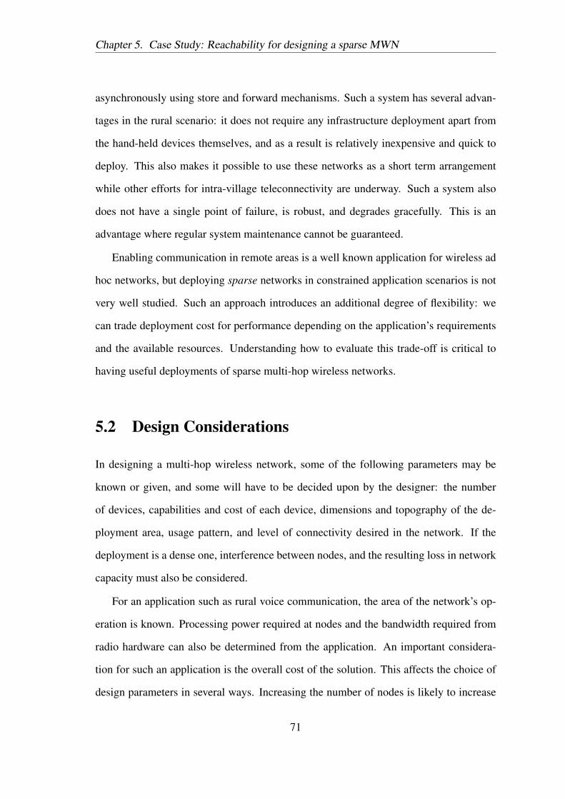
Figure 5.2: Reachability and Connectivity vs. N

To answer this question, a graph such as Figure 5.1 is useful. It plots reachability and

connectivity against R for 60 nodes. Each point on the graph is the average of 500

simulations. The graph tells us, for instance, that setting the value of R at 100m will

certainly not facilitate communication in the village. Similarly, settingR to a value above

600m is unnecessary since the network is already fully connected at that point. We can

set the value of R for any desired value of reachability or connectivity. However, as R

is increased, there will be a corresponding increase in the node’s power usage. When R

is in the region of the curve where the network’s connectivity or reachability is growing

rapidly, small changes in R can result in large changes in the extent to which the network

is connected.

5.3.3 Choosing N

• R is fixed at 300m for a specific device’s capabilities in the local terrain. How many

nodes are required to be operational in order to ensure that a villager who tries to

make a call to another succeeds on average 60% of the time?

This question can be answered from finding the value of N corresponding to a reachabil-

ity of 0.6. From the graph in Figure 5.2, we learn that we would need around 70 devices

operational in the area. (Note also that Figure 5.2 provides an illustration of our claim in

75


Figure 5.3: Determining R and N for a given reachability

Chapter 4 that reachability is more sensitive than connectivity for sparse networks. When

reachability is 0.6, the corresponding value of connectivity is not useful since it is still at

zero.)

An interesting observation can be made from Figure 5.1 regarding the behaviour of

the reachability and connectivity metrics. With R set to 400m, reachability is almost at

1, but connectivity does not reach 1 till R is around 600m. This implies that the extra

200m required to ensure full connectivity contributes very little towards increasing the

number of node pairs that can communicate. At the same time, the extra range comes at

a very high cost since transmission power varies as a power law function of distance.

5.3.4 R vs. N

Figure 5.3 shows the relationship between the values ofR andN required to keep reacha-

bility fixed at 0.2, 0.6 and 0.95. Note that as N decreases below a threshold, the required

value of R increases steeply. Given the maximum value R can take for a device, we can

find the minimum number of those devices required to be operational for achieving the

required reachability. As the network evolves, more nodes may join, or some nodes may

be switched off. If we are in a position to implement distributed power control at the

nodes, we can use curves like these to maintain reachability at a desired level.

76


In Chapter 6, we characterise reachability using an empirical regression model. We

have used this model to build a design tool for sparse MWNs called Spanner2. Given

three values from deployment area, reachability, R and N , it calculates the fourth. Data

points for Figure 5.3 have been generated using this tool.

5.4 Further observations

5.4.1 Network reach

Since the network we are studying is sparse, we would like to know if nodes are con-

nected only to nearby nodes. If all the node pairs that contribute to the reachability of the

network are located near each other, then the network would only be facilitating com-

munication between people who are already within easy reach. We use the following

theorem to find the span covered by a path.

Theorem 5.4.1: Let G = (V,E) be a graph in which every pair of nodes (u, v) ∈ V ×V

has a distance |uv|, and (u, v) ∈ E iff |uv| ≤ R. Then, if the shortest path between

some two nodes in V has k edges, k > 1, the sum of the distances of those k edges, L, is

bounded as: bk2cR < L ≤ kR.

Proof. The upper bound is trivially kR. L > kR would imply at least one of the k edges

being larger than R, which is not possible by definition.

When k = 2, let nodes u, v, w in order be the nodes on the shortest path. Then,

L = |uv| + |vw| cannot be less than or equal to R since this would imply (u,w) ∈ E.

This is clearly not possible since the nodes u, v, w define a shortest path. Therefore

L > R when k = 2. When k = 4 with a shortest path defined by nodes u, v, w, x, y in

order, |uw| > R and |wy| > R, implying L > 2R. Extending this argument for all even

2Available from http://www.it.iitb.ac.in/∼srinath/tool/rch.html

77


k, L > k2R. This same lower bound must also hold for the shortest path of odd length

k+ 1, since adding an edge cannot decrease L. Therefore, for all k > 1, L > bk2cR.

To find typical values of the shortest path, k, for the network under consideration, we

ran simulations with N = 70 and R = 300, and averaged the length of the shortest path

between every pair of connected nodes. The absolute maximum value we saw in any of

the 500 simulated network instances was 9.24, the minimum was 2.01, and the average

shortest path length was 5.24. From the above theorem, an average shortest path length

of around 5 implies a piece-wise linear distance greater than 600m, and at most 1500m in

the average case. This indicates that the network is capable of connecting pairs of nodes

that are not necessarily located near each other. The mean reachability observed in this

case was 0.6.

5.4.2 Mobility

To investigate the effect of mobility, with N = 70 and R = 300, nodes were made to

move at a speed between 0.5ms−1 and 2ms−1 following the random waypoint (RWP)

mobility model. The simulation time was 12 hours in which nodes moved to random

destinations, paused for half an hour, and then continued moving to another random

destination. This mobility pattern was chosen to approximate the movement of people

over one day.

We found that reachability had increased to 0.71 from the value of 0.6 observed for

the static network. This increase is likely due to the effect of the RWP mobility model. As

noted in Section 2.5.1, the RWP mobility model is known to change the initial distribution

of nodes and cause density waves. As a result, localised parts of the network tend to be

dense, causing an increase in the network’s connectivity properties.

78


Figure 5.4: With asynchronous communication

5.4.3 Asynchronous Communication

Asynchronous communication is particularly useful in sparse networks when routes are

difficult to find between source and destination. A message may be passed on to other

nodes in the vicinity of the source, and these nodes in turn propagate the message till it

reaches the destination. Thus, a message may travel from source to destination without a

complete path existing between them at any time. Message Ferrying [ZAZ04] and rout-

ing in delay tolerant networks [JFP04] are representative examples of such asynchronous

communication.

We extended the scenario from Fig. 5.1 to include some degree of asynchronous

communication. R was varied keeping N = 60. Nodes moved at a uniform velocity

of 5ms−1 without pause. For purposes of calculating reachability, a node pair was con-

sidered connected at simulation time t if a path, possibly asynchronous, existed between

the two nodes within t + 30 seconds. This translates to asking whether a packet with

a timeout of 30 seconds can be successfully transmitted between the two nodes using a

store and forward mechanism. Similarly, for connectivity, the network was considered

connected at a time instant t if all nodes could reach each other asynchronously within

time t + 30. Averaged values of 20 simulations of 500 seconds each are shown in Fig.

5.4. On average, nearly 80% of node pairs are connected before connectivity begins to

increase from zero. This indicates that sparse networks can achieve a significant degree

79


of communication by operating asynchronously, and further, that reachability is able to

capture this communication capability.

5.5 Conclusions

In this chapter we proposed sparse wireless multi-hop networks as being a possible means

for facilitating telecommunication within villages in India and discussed design consid-

erations. We made several simplifying assumptions in the case study, and these will have

to be addressed before such a solution can be considered practical. We also demonstrated

the use of reachability in evaluating design tradeoffs for such networks, from which we

draw the following conclusions:

• sparse MWNs can enable a significant degree of communication, and the extent of

communication achieved is even more substantial when a sparse network is capable

of mobility and asynchronous communication; and

• simulation studies in which we measured both reachability and connectivity indi-

cate that reachability is more sensitive to changes in network parameters, and hence

better suited for evaluating topological design considerations in sparse MWNs.

80

Chapter 6

Characterising Reachability

Recall that the reachability of a static network is defined as the fraction of connected node

pairs in the network. Using this definition we can calculate reachability for a network of

N nodes as1:


N2

) (6.1)

We consider a pair of nodes as connected if there is a path of length one or greater

between them. Note that for the same set of nodes, it is possible to have different values of

reachability for different instances of the network. A network for our purposes is defined

by the number of nodes, their bounding area, and the transmission ranges of the node.

The network’s reachability would be the average of reachability values across several

instances. This value is significant since it represents the probability that a random pair

of nodes in the network are connected by a possibly multi-hop path. When nodes are

mobile, the fraction of connected node pairs varies depending on node mobility, but a

single value can be obtained for any time instant. We can measure reachability for a

mobile network as the average of instantaneous reachability values measured at frequent

1The equation is repeated here for easy reference.

81

Chapter 6. Characterising Reachability

intervals during the operation of the network.

In this chapter we characterise reachability for a two-dimensional static network in

the finite domain with a uniform distribution of nodes2. The characterisation is also valid

for mobile networks in which the uniform distribution of nodes is preserved. The objec-

tive is to use the metric for topology design in sparse networks as shown in Chapters 4 and

5. In the rest of this chapter, we introduce the network model and notation used (Section

6.1), derive closed form expressions for two and three nodes in one dimension (Section

6.2), and present an empirical regression model for reachability based on simulated data

(Section 6.4).

6.1 Network model and notation

Our network model is as follows:

• N nodes are distributed uniformly at random in a d dimensional cube of side l;

• two nodes can communicate directly with each other if the distance between them

is not greater than R, the uniform transmission range of the nodes;

• since the network graph remains unchanged when R and l vary proportionally, we

combine the two into a normalised transmission range, r = R/l, without loss of

generality.

While this model takes a simplistic view of radio propagation, it promotes better de-

fined behaviour of topological properties, and is useful for an initial study. For a network

with N nodes, normalised transmission range r, and a mobility model denoted by M in a

cube of d dimensions, we denote the corresponding value of reachability as RchM,dN,r . In

this work, since we deal only with characterisation of the static case, we use the notation

2This work appears in [PI06a] and [PI].

82


RchdN,r. In the case of most interest, when d = 2, we drop the superscript altogether for

convenience and write RchN,r.

6.2 Analysis of small cases

In this section we derive closed form expressions for reachability of two and three static

nodes whose positions are distributed uniformly at random along a line of length l: Rch12,r

and Rch13,r. It is evident that results for these cases will be of limited practical use. The

main aim here is to attempt to gain a basis for a broader characterisation of reachability.

6.2.1 Rch12,r

Figure 6.1: Positions of a single node on a line segment

Let N1 and N2 be two nodes that can take positions uniformly at random on a line of

length l. Rch12,r is 1 when the two nodes are connected, and 0 when they are not. The

reachability for this network is therefore equivalent to the probability that two nodes with

transmission ranges R are connected when they are distributed randomly on a segment

of length l. (As this implies, reachability and connectivity are identical when a network

has two nodes.)

We define the coverage of a node as the length of the line segment that is covered by

the transmission range of the node. The probability that N1 and N2 are connected is then

83


given by the fraction of the length l that is covered by N1:

Rch12,r =

Coverage(N1)

l(6.2)

We first consider the case when l ≥ 2R. As seen in Figure 6.1, the coverage of N1

varies depending on where it is positioned on the line segment. The coverage of N1 is

2R if it is more than a distance R away from either end point of the line segment. If it is

placed in one of the edge segments of length R, its coverage on one side would remain

R, while the coverage on the other side would be between 0 and R. Considering all

positions along the edge segments equally likely, the coverage of N1 in an edge segment

is R for the side away from the edge, and the expected coverage is R2

for the side near

the edge3. Therefore, the total expected coverage of N1 on an edge segment of length R

is 3R2

, and the total coverage of N1 in the middle segment of length l − 2R is 2R. The

expected coverage of N1 across the line of length l is obtained by weighting the expected

coverages for edge and central segments with their relative lengths:

Coverage(N1) =

(2R

l

)(3R

2

)+

(l − 2R

l

)2R

=2Rl −R2

l, (l ≥ 2R).

For the case when 2R > l > R, we divide the line of length l into three segments of

lengths l − R, 2R − l and l − R. When N1 is located in the central segment of length

2R− l, its coverage is l because N1’s transmission range extends beyond the end-points

on either side. When N1 is located on either of the edge segments of length 2R − l, it

extends to a length R on the side of the farther end-point. On the side of the nearer end-

point, N1’s coverage is between l − R and, when it is exactly on the end-point, 0. The

expected value for coverage on the side of the nearer endpoint is (l − R)/2. Therefore,

3If c is a random variable representing coverage on the side near the edge, the expected coverage whenthe node is located in the edge segment of length R is 1

R

∫ R

0c dc or R

2 .

84


when 2R > l > R,

Coverage(N1) = 2

(l −Rl

)(R +

l −R2

)+

(2R− ll

)l

=2Rl −R2

l, (2R > l ≥ R).

Since the coverage is the same for both cases, we can write

Coverage(N1) =2Rl −R2

l, (l > R).

Substituting in Equation 6.2:

Rch12,r =

2R

l− R2

l2, (l ≥ R) (6.3)

= 2r − r2, (r ≤ 1). (6.4)

6.2.2 Rch13,r

Finding Rch13,r using the method applied in Section 6.2.1 is considerably more involved.

We proceed by enumerating the node configurations that are possible with three nodes on

a straight line. We then find the value of reachability for each of these configurations, and

then calculate expressions for the probability of occurrence of each of the configurations.

The sum of reachabilities across these configurations weighted by the probability of its

concurrence gives the expected value of Rch13,r. We formalise this notion below.

A network consisting of three nodes on a straight line must be in one of the following

configurations:

A. All three nodes are isolated

B. One node is isolated and the other two are connected

C. All three nodes are connected with one node being an intermediate node

85


D. All three nodes are directly connected to each other

If the three nodes are isolated as in Case A,Rch13,r is 0 by definition. In Case B, it follows

from our definition of reachability (Equation 6.1) that Rch13,r is 1

3. This is because one

node pair out of the possible three node pairs is connected. If the nodes are as in cases

C and D, Rch13,r is 1 since all possible node pairs are connected. The sum of Rch1

3,r

for each possible cases after weighting with the probability of concurrence of each case

gives us the expected value of Rch13,r:

Rch13,r = 0.P (A) +

1

3.P (B) + 1.P (C) + 1.P (D)

=1

3P (B) + P (C) + P (D). (6.5)

6.2.3 Rch13,r without edge effects

We first perform the analysis for N = 3 without accounting for edge effects. This means

we assume the coverage of a node to be 2R regardless of where it is located on the line.

Such an assumption is convenient since it allows us to illustrate the broad lines on which

analysis for N = 3 proceeds without the distraction of deriving exact coverages for edge

segments. In Section 6.2.4, we present an analysis for N = 3 that considers edge effects.

We enumerate the ways in which three nodes could come to be positioned on a

straight line, and calculate their probabilities. This is represented in the tree diagram

of Figure 6.2. At the root of the tree is the event where node N1 is located on the line

covering a length of 2R. At the next level of the tree are the exhaustive events X , Y

and Z, caused by a second node being placed on the line. At the third level are events

marked on the tree by subscripts of X , Y and Z, that are caused by a third node N3 being

placed on the line. We presently find the probabilities of these events, and use them to

find values of P (A), P (B), P (C) and P (D), which in turn can be used with Equation

6.5. Node N1 is positioned at an arbitrary point on the line segment, and it is assumed to

86


Figure 6.2: Tree diagram of outcomes for three nodes positioned on a line

cover a segment of the line that is 2R in length. Now, whenN2 takes a position uniformly

at random on the line, it can do so in three ways represented here by X , Y and Z.

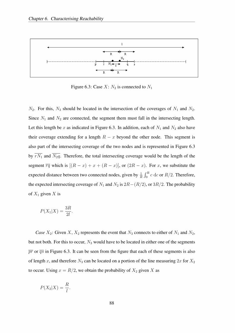
Case X: N2 connects to N1

For this, N2 will have to be located within the 2R coverage of N1. Since N2 takes its

position uniformly at random, the probability of this case occurring is given by P (X) =

2R/l.

Figure 6.3 illustrates Case X . The coverages of N1 is the distance between p and q,

and the coverage of N2 is the distance between r and s. We denote these by pq and rs

respectively.

Case X1: Given X , X1 represents the event that N3 directly connects to both N1 and

87


Figure 6.3: Case X: N2 is connected to N1

N2. For this, N3 should be located in the intersection of the coverages of N1 and N2.

Since N1 and N2 are connected, the segment them must fall in the intersecting length.

Let this length be x as indicated in Figure 6.3. In addition, each of N1 and N2 also have

their coverage extending for a length R − x beyond the other node. This segment is

also part of the intersecting coverage of the two nodes and is represented in Figure 6.3

by rN1 and N2q. Therefore, the total intersecting coverage would be the length of the

segment rq which is [(R − x) + x + (R − x)], or (2R − x). For x, we substitute the

expected distance between two connected nodes, given by 1R

∫ R0c dc or R/2. Therefore,

the expected intersecting coverage ofN1 andN2 is 2R−(R/2), or 3R/2. The probability

of X1 given X is

P (X1|X) =3R

2l.

Case X2: Given X , X2 represents the event that N3 connects to either of N1 and N2,

but not both. For this to occur, N3 would have to be located in either one of the segments

pr or qs in Figure 6.3. It can be seen from the figure that each of these segments is also

of length x, and therefore N3 can be located on a portion of the line measuring 2x for X2

to occur. Using x = R/2, we obtain the probability of X2 given X as

P (X2|X) =R

l.

88


Case X3: Given X , X3 represents the case that N3 connects to neither N1 nor N2.

For this to occur, N3 must be located anywhere along the line in Figure 6.3 except the

entire segment ps, whose length is 2R + x. Using x = R/2, we see that N3 can be

located anywhere along the line of length l except a segment of length 5R/2. We obtain

the probability of X3 given X as

P (X3|X) = 1− 5R

2l.

Case Y : N2 can only be connected to N1 through an intermediate node

SinceN1 andN2 cannot be connected directly,N2 must not be located in the 2R coverage

of N1. But it must be located close enough to N1 for N3 to potentially act as an interme-

diate node connecting N1 and N2. For this, N2 must be located at a distance between R

and 2R from N1. There are two such segments of length R on either side of N1, so the

total length along which N2 can be located for Case Y to occur is 2R. The probability of

this case occurring is therefore P (Y ) = 2R/l.

Figure 6.4: Case Y : N2 can only connect to N1 through an intermediate node

Case Y1: Given Y , Y1 represents the case where N3 connects N1 with N2. For this

to occur, N3 must be located in the intersection of the coverages of N1 and N2. This is

represented by the segment rq in Figure 6.4 whose length we denote as y. We have seen

that for Case Y to occur, N2 must be located at a distance between R and 2R from N1.

Since N2 is located uniformly at random along the line, the expected distance of N2 from

89


N1 is 3R/2. Using N1N2 = 3R/2, we obtain the value of y as R/2. Therefore

P (Y1|Y ) =R

2l.

Case Y2: Given Y , Y2 represents the case where N3 connects either one of N1 or N2. For

this to occur, N3 must be located in the segments pr or qs. From Figure 6.4 each of these

can be seen to be of length 2R − y. Using y = R/2, the combined length of the two

segments is obtained as 3R. Therefore

P (Y2|Y ) =3R

l.

Case Y3: Given Y , Y3 represents the case where N3 connects neither N1 nor N2. For this

to occur, N3 must be located on l outside the segment ps. The length of this segment can

be seen to be 4R− y, or, using y = R/2, ps = 7R/2. Therefore

P (Y3|Y ) = 1− 7R

2l.

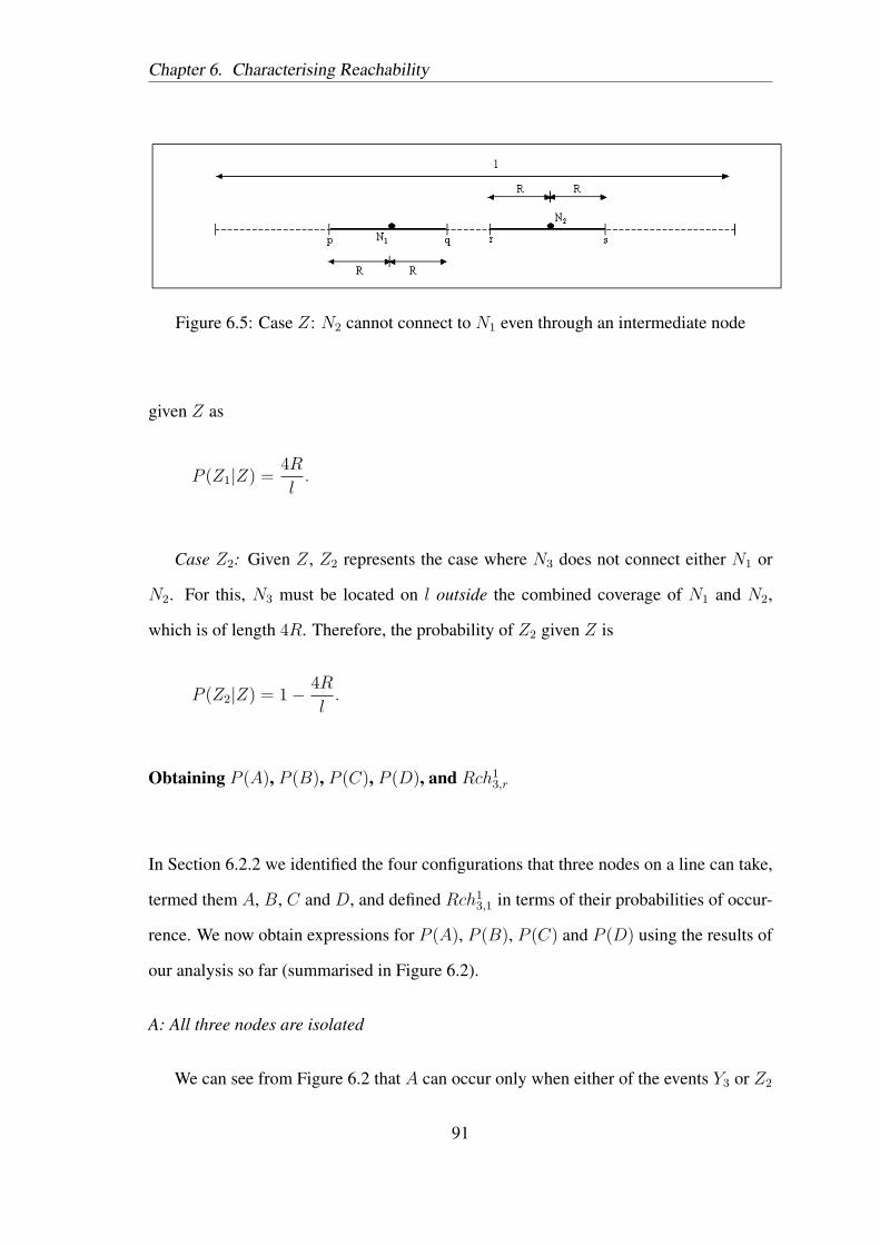
Case Z: N2 cannot connect to N1 even through an intermediate node

In order for N2 not to be directly connected to N1, it must not be located in the two

segments of lengthR on either side ofN1. ForN2 not to have a chance of being connected

to N1 through an intermediate node, a further segment of length R on either side of N1

must be excluded. Therefore, the total length in which N2 cannot be located is 4R. The

probability of Case Z occurring is therefore P (Z) = (l − 4R)/l.

Case Z1: Given Z, Z1 represents the case where N3 connects to either one of N1 or

N2. From Figure 6.5 we see that this can happen by N3 being located in either of the

segments pq or rs, together of length 4R. Therefore, we obtain the probability of Z1

90


Figure 6.5: Case Z: N2 cannot connect to N1 even through an intermediate node

given Z as

P (Z1|Z) =4R

l.

Case Z2: Given Z, Z2 represents the case where N3 does not connect either N1 or

N2. For this, N3 must be located on l outside the combined coverage of N1 and N2,

which is of length 4R. Therefore, the probability of Z2 given Z is

P (Z2|Z) = 1− 4R

l.

Obtaining P (A), P (B), P (C), P (D), and Rch13,r

In Section 6.2.2 we identified the four configurations that three nodes on a line can take,

termed them A, B, C and D, and defined Rch13,1 in terms of their probabilities of occur-

rence. We now obtain expressions for P (A), P (B), P (C) and P (D) using the results of

our analysis so far (summarised in Figure 6.2).

A: All three nodes are isolated

We can see from Figure 6.2 that A can occur only when either of the events Y3 or Z2

91


occur. Therefore:

P (A) = P (Y3) + P (Z2)

= P (Y3|Y ).P (Y ) + P (Z2|Z).P (Z)

=

(1− 7R

2l

)(2R

l

)+

(1− 4R

l

)(1− 4R

l

)(6.6)

Simplifying and using r = R/l,

P (A) = 1− 6r + 9r2 (6.7)

B: One node is isolated, and the other two are connected

From Figure 6.2 we see that B can occur only when one of X3, Y2 or Z1 occur.

Therefore:

P (B) = P (X3) + P (Y2) + P (Z1)

= P (X3|X).P (X) + P (Y2|Y ).P (Y ) + P (Z1|Z).P (Z)

=

(1− 5R

2l

)(2R

l

)+

(3R

l

)(2R

l

)+

(4R

l

)(1− 4R

l

)P (B) = 6r − 15r2 (6.8)

C: All three nodes are connected with one node being an intermediate node

C can only occur when either X2 or Y1 occur. Therefore:

P (C) = P (X2) + P (Y1)

= P (X2|X).P (X) + P (Y1|Y ).P (Y )

=

(R

l

)(2R

l

)+

(R

2l

)(2R

l

)P (C) = 3r2 (6.9)

92


D: All three nodes are directly connected to each other

D can only occur when X1 occurs. Therefore:

P (D) = P (X1)

= P (X1|X).P (X)

=3R

2l.2R

l

P (D) = 3r2 (6.10)

Note that P (A) + P (B) + P (C) + P (D) = 1. Since the probabilities have been

derived independent of each other, this validates that the events A, B, C and D, which

we have considered exhaustive, are indeed so.

Substituting for P (B), P (C) and P (D) in Equation 6.5 we get:

Rch13,r = 2r + r2 (6.11)

As l grows relative to R, the error caused by ignoring edge effects decreases, and

Equation 6.11 improves in accuracy.

6.2.4 Rch13,r with edge effects

Since quantifying the edge effect for every configuration of nodes is a painstaking task,

we use our experience with the analysis in the previous section to choose the smallest

number of cases that will allow us to obtain an expression for Rch13,r. Of the events A,

B, C and D, we saw that D is composed of a single sub-event (X1), both A and C are

composed on two sub-events (Z2 or Y3, andX2 or Y1 respectively), andB is composed of

three sub-events (X3 or Y2 or Z1). We therefore choose to rewrite Equation 6.5 in terms

of P (A), P (C) and P (D). Since we know that P (A) + P (B) + P (C) + P (D) = 1, we

93


substitute for P (B) in Equation 6.5 to obtain

Rch13,r =

1

3[1− P (A) + 2P (C) + 2P (D)]. (6.12)

Expressions for P (A), P (C) and P (D) in terms of r when l ≥ 4R are obtained as

follows. The approach used is similar to that used in deriving coverage for N = 2.

P (D): All three nodes are directly connected

As seen in Section 6.2.3, P (D) = P (X1). Here we will derive P (X1) considering node

placements towards the edge of the line. Note that P (X) with edge effects is equivalent

to Rch12,r which has been derived in Equation 6.3.

P (D) = P (X1)

= P (X1|X).P (X)

= P (X1|X).(2r − r2) (6.13)

We now find P (X1|X) with edge effects. Let x be the expected distance between two

directly connected nodes. LetN1 be the node closest to the left end of the line segment of

length l, and let N2 be the other node connected to N1 on its right. Note that the coverage

area for N3 to be connected to both of them is the length between the two nodes, x, and

an overlap of R − x on N2’s right and an overlap of R − x on N1’s left. Here, we also

need to accommodate for the reduction of this overlap when the two nodes are near the

end segments of the length of operation, as we did for the case N = 2. Coverage for the

initial R − x segment of l is (R − x)/2 to N1’s left, x in between, and R − x to N2’s

right. Coverage for the rightmost segment of length R, after compensating for reduction

of overlap is obtained as 5R/4, and coverage for the central l−2R+x segment is 2R−x.

94


The expected coverage is:

(R− x

2+ x+R− x

)(R− xl

)+

(l − 2R + x

l

)(2R− x) +

(R

l

)(5R

4

)

Substituting x = R/2 (we do not consider edge effects for x itself, since the resulting

error is small and allows us to obtain an equation of lower degree), and dividing by l:

P (X1|X) =3R

2l− 3R2

8l2

Taking r = R/l and substituting in Equation 6.13,

P (D) =

(3r

2− 3r2

8

)(2r − r2) (6.14)

P (C): Three nodes are one-hop connected

As seen in Section 6.2.3, P (C) = P (X2) + P (Y1). Here, we derive P (X2) and P (Y1)

without ignoring node placements towards the edge of the line.

P (C) = P (X2) + P (Y1)

= P (X1|X).P (X) + P (Y1|Y ).P (Y ) (6.15)

We have already seen that Rch12,r is identical with P (X).

P (X2|X): Let the expected distance between two connected nodes be x. Since N1

and N2 are given to be connected, N3 can be one-hop connected with N1 only by being

located to the right of N2 in a segment that does not overlap with N1’s coverage. This

segment is of length x. We do not consider N3 being located to the left of N1 since that

case is covered by the symmetrical nature of our analysis. (The analysis proceeds from

left to right of the line segment with N2 always to the right of N1. We could perform

another analysis proceeding from right to left and weight both results by half, but the

95


two analyses would be identical except for the nomenclature of the nodes.) The segment

of length l is divided into four segments of length R − x, 2x, l − 2R − x, and R, from

left to right to account for boundary conditions. After identifying the coverages for each

of those segments, taking the product of coverages and segment lengths, summing, and

substituting x = R/2, we get the coverage within which a node would one-hop connect

two already connected nodes as R− (R2/l). Substituting r = R/l and dividing by l,

P (X2|X) = r − r2

P (Y ): We find the probability of two nodes being located such that they are not

connected, but can possibly be connected. Note that the criterion for this is that the two

nodes should be separated by at least a distance of R, and not more than a distance of

2R. We call the length in which N2 can be positioned to potentially satisfy condition Y

as the placement length4 for N2. For ease of analysis we divide the line on which the

nodes are located into five segments: two segments of length R from each of the end-

points, and a central segment of length l − 4R. We do this because the placement length

of N2 varies depending on where N1 is located. We therefore calculate this length when

N1 is located in each of these segments, and we weight it by the length of the respective

segment to get the expected placement length of N2.

When N1 is located on the leftmost segment of length R, N2 can only be positioned

in a segment of length R after leaving a gap of R. Therefore, the placement length of N2

for this part of the line is R.

When N1 is located on the next segment on length R, N2 can be placed on a segment

of length R after leaving a gap of R as for the first segment. In addition, N2 can also be

placed to the left of N1 after leaving a gap of R. Depending on where N1 is located on

4Placement length is analogous to the term coverage used in other parts of this analysis. We do not usethe term coverage here because there is no actual overlap of transmission ranges of nodes at this stage ofthe analysis.

96


the second segment, this length can vary from 0 to R, giving an expected value of R/2

when the nodes are uniformly distributed. The total expected placement length for N2

when N1 is located in this segment is 3R/2.

When N1 is in the central segment of length l − 4R, N2 can be located in a segment

of length R after a gap of R either to the left or right of N1. The expected placement

length is therefore 2R.

The placement lengths for N2 for the remaining two segments are the same as those

for the first two segments by symmetry. Weighting by the relative length of the segments,

we find the expected placement length for N2 as:

(R

l

)R +

(R

l

)(3R

2

)+

(l − 4R

l

)2R +

(R

l

)(3R

2

)+

(R

l

)R

Dividing by l to obtain P (Y ), substituting r = R/l, and simplifying we get:

P (Y ) = 2r − 3r2

P (Y1|Y ): Let y be the expected distance between nodes that are not connected, but

can be connected by a third node. Then, y ranges from R to 2R with an expected value

of 3R/2. The expected intersecting coverage of the two nodes in which N3 must be

positioned to satisfy condition Y1 is 2R − y. Substituting y = 3R/2, this coverage is

R/2. Therefore, after dividing by l, we get

P (Y1|Y ) =

(r

2

)

Substituting the above obtained equations in Equation 6.15 we get

P (C) = (r − r2)(2r − r2) +

(r

2

)(2r − 3r2) (6.16)

97


P (A): All three nodes are isolated

As seen in Section 6.2.3, P (A) = P (Y3) + P (Z2). Here, we derive P (Y3) and P (Z2)

without ignoring node placements towards the edge of the line.

P (A) = P (Y3) + P (Z2)

= P (Y3|Y ).P (Y ) + P (Z2|Z).P (Z) (6.17)

We have already seen that P (Y ), the probability of two nodes falling such that they are

not connected, but can be connected by a third node is 2r − 3r2.

P (Y3|Y ): We find the coverage length within which the third node could be con-

nected to one or both the nodes, and obtain its complement as the probability that the

third node will not be located in this coverage length. Let the line be divided into four

segments of length R, l − 3R, R and R. Let N1 be the node near the leftmost endpoint

of the line. From condition Y , we know that N2 must be located between R and 2R to

N1’s right. When N1 is in the first segment, the total coverage of the two nodes consists

of the expected coverage of N1’s to its left (R/2), the expected distance between N1 and

N2 (3R/2), and N2’s coverage to its right (R). When N1 is in the second segment of

length l − 3R, the coverages remain the same except for N1’s coverage to its left, which

increases to R. When N1 is in the third segment of length R, the total coverage is the 2R

constituted by the last two segments along with the expected coverage of N1 extending

to its left, which is R/2. Note that since N1 is the leftmost node, and since N2 must be

a distance of at least R to its right, N1 cannot be located in the last segment. Weighting

the coverages by relative length of the segments, we get

(R

l

)(R

2+

3R

2+R

)+

(l − 3r

l

)(R +

3R

2+R

)+

(R

l

)(R

2+ 2R +

R

3

)

Simplifying and dividing by l gives us the probability of N3 being connected to either or

98


both of N1 and N2. Taking the complement and substituting r = R/l gives us:

P (Y3|Y ) =

(1− 7r

2+

14r2

3

)

P (Z): In order not be connected by an additional node, N1 andN2 must be located at

least 2R away from each other. To calculate P (Z) we first find the expected placement

length for N2. For ease of analysis, we divide the line segment of length l into three

segments of length 2R, l − 4R, and 2R.

Depending on the position of N1 in the leftmost 2R, N2 must be positioned between

l − 2R and l − 4R from the rightmost end for condition Z to be satisfied. The expected

placement length for N2 when N1 is in the leftmost segment is therefore l − 3R.

When N1 is in the central segment of length l − 4R, N2 can be positioned in the

rightmost segment varying in length from l − 4R to 0, depending on the position on N1.

N2 can also be positioned in parallel in the leftmost segment varying in length from 0 to

l − 4R. Therefore, the placement length for N2 is fixed at l − 4R for this case.

The placement length for N2 for the remaining segment is same as that for the first

segment by symmetry. Weighting by the relative length of the segments, we find the

expected placement length for N2 for case Z as:

(2R

l

)(l − 3R) +

(l − 4R

l

)(l − 4R) +

(2R

l

)(l − 3R)

Dividing by l to obtain P (Z), substituting r = R/l, and simplifying we get:

P (Z) = 1− 4r + 4r2.

P (Z2|Z): We find the combined coverage length of two nodes that cannot be con-

nected to each other by a third node, and obtain the probability that the third node will

not be located anywhere in that coverage area. For this, we find the total coverage that the

99


third node should not be located in. N1 and N2 have no overlap in their coverages since

they satisfy condition Z. We divide the line into three segments of lengths R, l− 2R and

R. When either of N1 or N2 is in the central l − 2R segment, its coverage is 2R. When

it is in one of the edge segments, its expected coverage is R/2 on the side closer to the

endpoint, and R on the side closer to the centre, making a total of 3R/2. Weighting by

the relative size of the segments and doubling to account for both nodes gives us total

coverage of N1 and N2 as

2

[(2R

l

)(3R

2

)+

(l − 2R

l

)2R

]

We now divide by l, substitute r = R/l and simplify to obtain the probability of N3

connecting to either N1 or N2 as 4r + 2r2. The complement of this gives us:

P (Z2|Z) = 1− 4r + 2r2.

Substituting the above obtained equations in Equation 6.17 we get:

P (A) = (1− 4r + 2r2)(1− 4r + 4r2) +

(1− 7r

2+

14r2

3

)(2r − 3r2) (6.18)

Now, we have obtained expressions for P (D), P (C), and P (A) in Equations 6.14,

6.16 and 6.18. These along with Equation 6.12 constitute analytical expressions for

Rch13,r with edge effects factored in.

Concluding note on analysis of Rch13,r

As seen earlier, Equations 6.7, 6.8, 6.9 and 6.10 give us P (A), P (B), P (C) and P (D)

without taking edge effects into account. This corresponds to the case when l >> R.

Equations 6.14, 6.16 and 6.18 give us P (D), P (C) and P (A) for the case when l > 4R.

Both these sets of equations yield polynomials in r. It is interesting to note that the coeffi-

100


cients of the first few terms remain the same in both sets. That is, the effect of considering

edge positions of nodes is to add higher order terms to the resulting equations.

Table 6.1 shows analytical and simulated values when r = 0.1 for P (A), P (B),

P (C), P (D) and Rch13,r. The first column shows values obtained using equations 6.7,

6.8, 6.9 and 6.10. In the second column, the values of P (A), P (C) and P (D) are ob-

tained using equations 6.18, 6.16 and 6.14, and these values are used to determine P (B).

In both the analytical columns, the value of Rch3,0.1 is obtained using Equation 6.12.

The values in the third column of Table 6.1 are from simulations conducted in Sim-

ran. Here Rch3,0.1 is obtained as the mean reachability across 10, 000 network instances

of three uniformly distributed nodes. Each instance can be classified as an event of type

A, B, C or D using the average hop count returned by the simulator for that instance.

Probability for each event was calculated as the fraction of instances satisfying the event

condition. For example, of the 10, 000 instances simulated, 4338 had two nodes con-

nected and one node isolated. This lets us calculate P (B) = 0.4338. Note that the values

in the second column, where edge effects are considered in the analysis, are closer to

simulated values. Our main aim in performing the analyses for Rch12,r and Rch1

3,r was to

Table 6.1: Analytical and Simulated values for r = 0.1

Analytical (l >> R) Analytical (l > 4R) SimulatedP (A) 0.49 0.5152 0.5122P (B) 0.45 0.4314 0.4338P (C) 0.03 0.0256 0.0261P (D) 0.03 0.0278 0.0279Rch1

3,0.1 0.21 0.1972 0.1982

investigate any structural properties of their derivations that could be exploited to obtain

exact expressions for Rch1N,r, and perhaps even Rch2

N,r which is the case of most inter-

est. The analysis performed for N = 3 required the handling of multiple cases, and was

significantly more involved than the analysis for N = 2. Carrying the analysis beyond

101


N = 3 would entail extending the tree diagram of Figure 6.2 to further levels. However,

such a probabilistic analysis for N > 3 would have to account for a staggering multiplic-

ity of cases, with many involving the calculation of multiple overlapping coverages. We

can conclude that this method is impractical for applying to larger values of N , and other

methods will have to be explored to characterise reachability for larger values of N .

6.3 Modelling RchN,r in the finite domain

There is work that gives asymptotic probabilistic bounds on connectivity in a one-dimensional

network by characterising the conditions required for a single node to be left out of the

connected component [SB02, SBV01]. Such an approach is difficult to use with reach-

ability since the metric by definition tries to capture communication capabilities in a

network that can be separated by disconnections. In any case, asymptotic results for one

dimensional networks, while of theoretical interest, are unlikely to be of practical use in

networks with smaller numbers of nodes.

If theN nodes form k components withmi nodes in the ith component, we can rewrite

Equation 6.1 as

RchN,r =

∑ki=1

(mi2

)(N2

) =

∑ki=1mi(mi − 1)

N(N − 1)(6.19)

It may be possible to use results for number of components and distributions of nodes for

a Random Geometric Graph [Pen03] to obtain asymptotic bounds (asN tends to infinity)

for RchN,r.

However, since sparse networks often involve small numbers of nodes, we are par-

ticularly interested in characterisations of RchN,r in the finite domain. Since we can

generate accurate data for RchN,r from simulations, we choose to obtain a finite domain

characterisation using empirical regression.

102


6.4 Empirical modelling of RchN,r in the finite domain

We explored data from simulations to see if reachability obeyed any known growth mod-

els. For this, we studied the relationship between r and RchN,r for various values of

N . We chose r (rather than N ) as our independent variable since it is continuous and

allows greater precision in choosing data points. That is, it allows us to obtain simulated

values for RchN,r at arbitrarily close intervals of r. RchN,r was observed to grow sig-

moidally from zero at r = 0 and reach an asymptote of one for some value of r. Plots of

RchN,r versus r were seen to be consistent in this regard for different values of N . After

a visual comparison with known growth models that explained this behaviour, we found

several candidates for modelling RchN,r. We conducted an initial round of regression

analysis using each of those models and selected the logistic growth model because it

consistently fit the simulated data for a wide range of r and N values with high accuracy.

Among models considered and rejected were power law models, sum of exponentials,

the Gompertz model, and various logarithmic functions as described in [Rat93].

The model for RchN,r is a function in terms of N and r, and is represented by

Rch(N, r).

6.4.1 The Logistic Growth Curve

The logistic model is often used to fit sigmoidal curves with a lower asymptote of zero

and a finite upper asymptote. Its most popular application has been in modelling the

growth of populations over time. Intuitively, logistic growth models a system that grows

rapidly beyond a threshold, and slows down as it approaches its maximum limit. Figure

6.6 shows a logistic curve expressed by the equation:

y =k

1 + eα−βx(6.20)

103


where k is the limiting value that y can take, β is the maximum rate of growth, and α

is a constant of integration [Kin82]. The curve is skew-symmetric and has a point of

inflexion at x = α/β, y = k/2, where the growth rate is maximum [Rat93]. We use the

Figure 6.6: A general logistic curve

logistic equation to model the growth of RchN,r as r increases for a fixed value of N .

Since the maximum value of reachability is one, it becomes our upper asymptote. α and

β are found to increase monotonically with N , and we denote them by α(N) and β(N).

We use Equation 6.20 in the form:

Rch(N, r) =1

1 + eα(N)−β(N)r(6.21)

Figure 6.7 shows the close correspondence between simulated data and Equation 6.21

for the case N = 100. The values of α(100) and β(100) used were 9.58 and 79.2

respectively. We see how these values were obtained in Section 6.5.

6.5 Simulation and Regression Modelling

After having identified reachability as consistent with the logistic model, our approach

towards characterising RchN,r was as follows:

104


• We conducted extensive simulations to obtain data that represented the growth of

RchN,r from 0 to 1 as r increased, while keeping N fixed.

• We used Equation 6.21 as a regression function for simulated data, and obtained

the coefficients α and β for the corresponding value of N . This allowed us to

characterise reachability as a function of r for one value of N .

• We repeated the above two steps for values of N ranging from 2 to 500, and per-

formed a second level of regression on the estimated values of α(N) and β(N).

This gave us a set of equations expressing reachability as a function of N and r for

values of N ranging from 2 to 500.

Figure 6.7: Logistic fit for N=100

6.5.1 Simulations

We conducted extensive simulations in Simran to generate the data required for fitting

the regression function. Since we were looking to characterise reachability for small to

medium sized networks, we chose 55 values of N between 2 and 500 as representative

points. For each of these values of N , we varied r in increments from zero to a value

where reachability was at its maximum value of one. For each such value of r, we

105


conducted simulations over 1000 randomly generated network graphs and calculated the

mean value of RchN,r across those instances.

We know that the error of the mean is within 1.96s/√n with 95% confidence where

s is the standard deviation of the samples, and n is the number of samples [Jai91]. A

worst case bound for s would be the case when the samples are uniformly distributed in

the interval [0, 1]. The variance for a uniform continuous distribution in the interval [a, b]

is given by (b− a)/12 [Tri01]. The worst case standard deviation for the interval [0, 1] is

therefore given by s =√

1/12 = 0.2887. Using this value of s, and with n = 1000, we

find that the error in the mean is within 0.018 with a confidence of 95%.

At the end of our simulations, we had 55 tables each containing r and reachability

values for the corresponding value of N . For illustration, one of these tables, for N=60,

is shown in Table 6.2.

6.5.2 Fitting the Logistic Curve

Our next step was to fit each of those 55 tables of values to Equation 6.21. We trans-

formed the non-linear equation to a linear form in order to use the linear least-squares

regression. Applying logarithms to both sides of Equation 6.21 we get:

log

(1

Rch(N, r)− 1

)= α(N)− β(N)r

Substituting t = log(

1Rch(N,r)

− 1),

t = α(N)− β(N)r

which allows us to estimate α(N) and β(N) using linear least-squares regression.

We estimated α and β for each of the 55 selected values of N . Goodness of fit as

measured by the R-squared statistic was close to 1 when averaged, with the lowest value

being 0.996. This corroborates the close agreement of simulated values and the fitted

106


equation seen in Figure 6.7. At this point, we obtained a table with estimated α and β

values for the 55 values of N chosen. Some rows of this table are shown in Table 6.3.

Table 6.2: N = 60r Rch60,r

0.11 0.0973067650.12 0.1447819290.13 0.2143242980.14 0.3135225690.15 0.4362045080.16 0.5723688960.17 0.7030841600.18 0.8113259840.19 0.8802966080.20 0.928937296

Table 6.3: N with corresponding α and βN α(N) β(N)2 3.255884789 6.2837368185 3.977056234 9.87063814010 4.691024580 14.53923918. . .. . .

55 8.145698174 50.9854386760 8.263521833 53.85171640. . .. . .

175 11.47178670 124.4936168200 12.03414482 138.8969787

. . .

. . .450 16.21675101 278.7307447500 16.69687608 302.2307067

6.5.3 Fitting the Logistic Coefficients

Having estimated the logistic coefficients α(N) and β(N) for several values of N , we

performed a second level of regression on the estimated coefficients to express α(N) and

β(N) in terms of N . Doing this allows us to interpolate α(N) and β(N) for values of

107


Figure 6.8: Estimated and fitted α

N we have not simulated, and lets us express α(N) and β(N) concisely in terms of N .

This can also reduce error by staying faithful to a general trend, mitigating the effect of

any anomalous data points.

We fit values of α to a sum of exponentials function, and values of β to a sixth degree

polynomial. In the absence of physically significant models, we chose models that gave

us maximum accuracy. The expressions in terms of N for 2 ≤ N ≤ 500 are:

α(N) = 3.004 + 3.815(1− e−4.091×10−2N)

+15.4(1− e−2.055×10−3N) (6.22)

β(N) = 5.141 + 0.9421N − 2.597× 10−3N2

+8.42× 10−6N3 − 1.37× 10−8N4

+1.058× 10−11N5 − 3.209× 10−15N6 (6.23)

Figures 6.8 and 6.9 plot the estimated values of α and β along with the curves repre-

sented by equations 6.22 and 6.23.

108


Figure 6.9: Estimated and fitted β

6.5.4 Validation

Equations 6.21, 6.22 and 6.23 form a model for reachability. Given a value of N and r,

we obtain the corresponding value of reachability as follows:

• obtain α(N) and β(N) by substituting N in equations 6.22 and 6.23; and

• substitute α(N), β(N) and r in Equation 6.21.

We chose 20 values of N between 2 and 500 at random, which were not among the

55 values of N chosen for the regression model. For each value of N , we chose five

values of r that would roughly correspond to a reachability value between 0.05 and 0.95.

This choice of r is necessary because a random selection of r is very likely to result in

a reachability of either zero or one, since reachability takes on values in between only

for a narrow range of values of r. We calculated the reachability corresponding to these

hundred pairs ofN and r values using equations 6.21, 6.22 and 6.23, and compared them

with values obtained from simulation. We calculated absolute and relative errors between

the simulated and estimated values of reachability. We found an average relative error of

3.5% in the model. We did not observe a single instance where the value of reachability

predicted by the model was in error by more than 0.05.

109


6.6 Extending the model

As N grows, smaller changes in r suffice for RchN,r to increase from a value near 0

to a value near 1. For example, when N = 10, the increase of Rch10,r from 0.1 to 0.9

corresponds to an increase in r of 0.3. But when N = 500, it corresponds to an increase

in r of only 0.015. As N grows larger, RchN,r begins to resemble a step function by

transitioning from a value of almost 0 to a value of almost 1 at a threshold value of r.

Such phase transition behaviour [KWB01] is a known property of multi-hop networks,

and the critical transmitting range is a well-studied problem for connectivity (Section

2.2.2).

In our model, the transition of Rch(N, r) for large values of N takes place at g(N) =

α(N)β(N)

which is the point of inflexion for the logistic curve. Note that in figures 6.8 and

6.9, the shape of the curves seems relatively stable for N greater than 200. We use data

for N between 200 and 500 to find a rough estimate for the critical transmitting range for

Rch(N, r) up to N = 1000. We approximate α(N) using a simple exponential function,

and β(N) using a linear function as

α(N) = 16.16(1− e−1.947×10−3N) + 6.658 (6.24)

β(N) = 27.8844 + 0.5522N (6.25)

for 500 ≤ N ≤ 1000. While these estimates do not exactly predict the point of inflexion,

they are close enough that setting r = g(N)−0.01 results in aRch(N, r) value close to 0,

and setting r = g(N) + 0.01 results in a Rch(N, r) value close to 1. Table 6.4 illustrates

this: the second column contains g(N) values obtained from equations 6.24 and 6.25,

and the third and fourth columns contain RchN,r values obtained from simulations by

setting r to g(N)− 0.01 and g(N) + 0.01 respectively.

110


Table 6.4: Beyond N = 500

N gN=αNβN

Rch(N,gN−0.01) Rch(N,gN+0.01)

500 0.055 0.0515 0.9418600 0.0495 0.0315 0.9470700 0.0451 0.0201 0.9518800 0.0413 0.0129 0.9518900 0.0381 0.0086 0.9515

1000 0.0354 0.0060 0.95051200 0.0308 0.0031 0.9414

6.7 Using the model: Spanner

We have presented a model for reachability to be used for estimating trade-offs between

number of nodes, transmission range, and required communication capability in wireless

multi-hop networks. To this end, we have built a design tool, Spanner (Sparse network

planner), incorporating the reachability model presented in this chapter. Given three

values from the number of nodes in the network, N , their uniform transmission range, R,

the side of the square area of operation, l, and the reachability, Rch, Spanner computes

the fourth value. A brief description of the tool follows.

Spanner is implemented as a C program invoked through a web server5. Three of

four values from N , R, l, and Rch are entered in a browser, and the value of the fourth

is computed. When N is given, Spanner first computes α(N) and β(N) using equations

6.22 and 6.23. It then solves for the value to be found by substituting in appropriate

forms of Equation 6.21. If Rch is to be found:

Rch =1

1 + eα(N)−β(N)(Rl)

5Spanner is online at http://www.it.iitb.ac.in/∼srinath/tool/rch.html

111


When R or l are to be found:

R

l=α(N)− log(1−Rch

Rch)

β(N)

The computation is a little different when N is to be found from R, l and Rch. N

cannot be directly solved because that would require us to know α and β which are

functions of N . Therefore, we write Equation 6.21 as:

α(N)− β(N)

(R

l

)= log

(1−RchRch

)

Since N is known to be between 2 and 500, we use binary search to obtain the N value.

An example of Spanner’s use can be seen in the case study in Chapter 5 where data

points in Figure 5.3 have been generated using this tool.

6.8 Handling model limitations

6.8.1 Idealised wireless propagation

The assumptions made regarding wireless propagation are idealised, and reachability

measured in a real deployment would almost certainly be lower than the value obtained

by using our model. One way to factor this knowledge into using the model for net-

work design would be to choose parameters conservatively. For instance, the value of

reachability obtained using the model could be treated as the upper bound for an actual

deployment. Or, if the model stipulates the transmission range required for a desired

level of reachability, it could be treated as the minimum required range.

6.8.2 Square area of operation

We have assumed a square area of operation for deriving the reachability model in this

chapter. It is not evident how this can be applied for a rectangular area of operation.

112


In Chapter 7, we demonstrate that connectivity properties for a network (such as con-

nectivity and reachability) vary when the shape of the operational area is changed. We

also provide analytical results for obtaining the side of a square area that has connectiv-

ity properties similar to a given rectangular area when all other network parameters are

fixed. Such a transformation could be used to apply the reachability model presented

here to rectangular networks.

6.8.3 Mobility

The results we have obtained in this chapter have been for a static network. In a static

network, a probabilistic value of reachability for a network is of limited use because the

specific network instance we obtain could have a different reachability value. But in the

presence of mobility and asynchronous communication, the measured value of reacha-

bility would tend towards its expected value over time. As evidenced by Figure 5.4 in

Chapter 5, a sparse MWN can support a significant degree of communication by operat-

ing asynchronously. Since reachability is able to effectively capture this communication

ability, it is in the design of such networks that reachability would be most useful.

Note that it is not mobility itself that prevents us from applying a model obtained from

static networks — it is what mobility does to the underlying distribution of nodes. Since

we have assumed a uniform distribution of nodes while obtaining the reachability model

in this chapter, it is also applicable to a mobile network whose mobility model results

in a uniform distribution of nodes. Therefore, it cannot be used with a mobility model

such as random way-point which causes non-uniform distributions of nodes [BRS03],

but it can be used with a mobility model such as random direction [RMSM01], which

is known to preserve a nearly uniform distribution of nodes [Bet02]. There is also work

that allows us to determine the stationary distributions for the locations of mobile nodes

[NC04, BRS03, BV05]. This distribution is a function of the mobility model used and its

parameters. It should also be possible to use the models obtained here when the stationary

113


distribution of mobile node locations is close to the uniform distribution. When this is

not the case, or when asynchronous communication exists between nodes, it is advisable

to use simulation.

6.9 Concluding remarks

In this chapter we gave a finite domain empirical characterisation of reachability for a

uniform distribution of nodes in a square area. Though the characterisation was obtained

for a square network, it is also applicable to mobile networks where the uniform distri-

bution of nodes is maintained. We also incorporated the obtained model in Spanner, a

design tool for sparse MWNs. Given three values from the number of nodes in the net-

work, N , their uniform transmission range, R, the side of the square area of operation, l,

and the reachability, Rch, Spanner computes the fourth value.

The use of the reachability characterisation for topology design in sparse MWNs can

perhaps be best illustrated by revisiting one of the design questions raised in the case

study of Chapter 5:

• If nodes in an MWN to be deployed in an area of 2000m x 2000m have a transmis-

sion range of 300m, how many nodes will be required to ensure that around 60%

of node pairs in the network can communicate at a given time?

To answer the above question, we had simulated the network scenario for various

values of N , and plotted a curve of reachability against N (Figure 5.2). We then deter-

mined that the value of N corresponding to a reachability of 0.6 was around 70. This

method of obtaining the answer is time consuming: the curve has 25 points, each of

which is the averaged value of 500 simulations. Further, if any of the network param-

eters change, the entire process would need to be repeated. In contrast, we can use the

reachability characterisation presented in this chapter to answer the same question easily

114


and quickly. Entering l = 2000m, R = 300m and Rch = 0.6 in Spanner (Section 6.7),

we get N = 69. Other combinations of parameters too can be evaluated similarly.

115


116

Chapter 7

Edge effects on Connectivity Properties

In chapters 3 and 6, we obtained empirical models for connectivity and reachability for

nodes in a square area of operation. While the assumption of a square area of operation is

common in work relating to connectivity properties of multi-hop networks, it is not clear

how analytical or empirical results obtained for a square area will apply to a more general

rectangular area. In this chapter we show that results obtained for a square area do not

necessarily apply even to similar rectangular areas: we present simulation results that

show reachability and connectivity varying for networks with the same area of operation,

but with differing geometries. One reason for this is the change in expected coverage

of a node as the shape of the operating area changes. We quantify expected coverage

for a single node in a rectangle and describe how it can be applied in extending results

obtained for square areas to rectangular areas.

7.1 Motivation

It is known that nodes at the boundaries of operating regions must be treated differently

from other nodes when dealing with topological and connectivity properties. For in-

stance, [IB05] mentions that nodes at the boundaries have fewer neighbours, and that

117

Chapter 7. Edge effects on Connectivity Properties

this can have a significant impact on network properties. In some studies, nodes are as-

sumed to be operating on a toroidal region to avoid handling special cases introduced by

edge effects [DB01]. A common feature in both finite domain and asymptotic analyses

of connectivity is the parametrisation of the network in terms of node density since this

subsumes both number of nodes and the area of operation [TFL03]. Further the area of

operation may be considered to be an d-cube for convenient generalisation across one-,

two-, and three-dimensional networks [SB02, SBV01, SB03]. However, such results can

be misleading when applied out of context to a rectangular area of operation.

The graph in Figure 7.1 plots simulation results for connectivity and reachability

against rectangularity in a static multi-hop network. We define rectangularity as the ratio

of length to breadth. We started with a square area of operation of 2 square units, with

30 nodes, each with a uniform transmission range of 0.4 units. We proceeded to increase

the ratio of length to breadth while keeping area and the number of nodes fixed. Hence

the curves in Figure 7.1 are for a network with constant node density, but with changing

geometry of the area of operation. The increase in rectangularity results in a decrease in

connectivity and reachability. This can be intuitively understood by imagining that each

node has a transmission area around it represented by the circle with transmission range

as its radius. The node can communicate directly with any other node present in the

transmission area. For any node, being present near the edge of the area of operation ef-

fectively means that some part of the transmission area is not utilised for communication

with other nodes. It can be shown that a rectangle has a larger perimeter than a square

of equal area. This causes a larger part of the nodes’ transmission area to fall outside the

area of operation, contributing to a decrease in connectivity properties.

In this chapter we quantify this edge effect using the notion of the effective ‘coverage’

of a node within a rectangular area of operation. Since coverage gives us the average

number of neighbours per node which in turn has been shown to determine connectivity

and reachability, we can use coverage to obtain the square equivalent of a network with

118


a rectangular area of operation 7.3. This provides a way to apply results obtained for

networks with square areas of operation to networks with rectangular areas of operation.

Figure 7.1: Connectivity properties change with rectangularity

7.2 Quantifying the edge effect for a single node

We derive exact expressions for expected coverage of a single node with transmission

rangeR, in a l×b rectangle. We are interested in determining expected coverage because

it allows to to quantify the extent of the edge effect. The expected coverage is also

closely linked to connectivity: dividing the expected coverage for one node by the area

of the rectangle gives us the probability that another similar node introduced at a random

position in the rectangle is connected to the first node. That is, it gives us an exact

expression for connectivity of two nodes in a rectangular area. We use this expression in

Section 7.3 to deal with larger networks.

We assume that the node under consideration has a transmission range of R, and can

be present with equal probability at any point within a rectangle of dimensions l× b. We

define:

119


Figure 7.2: Edge effects on a node’s radio coverage

Coverage of a node as the area of the circle of radius R around it that lies within the

rectangular area of operation.

For convenience of analysis we divide the rectangle into three regions. Figure 7.2 shows

these regions:

• Region 1 consists of the central portion of the rectangle where the coverage of the

node is the entire area of the circle around the node.

• Region 2 consists of a band of width R inside the perimeter of the rectangle, in

which a part of the node’s coverage area is circumscribed by exactly one of the

edges of the rectangle.

• Region 3 consists of squares of side R at each vertex of the rectangle, and repre-

sents the region where portions of the node’s coverage area are circumscribed by

two intersecting edges of the rectangle.

120


If τ1, τ2, and τ3 are the expected coverages in regions 1,2, and 3, the overall expected

coverage, τ , is given by weighting each of the coverages with the area of the correspond-

ing region, and dividing by the area of the rectangle:

τ =τ1(l − 2R)(b− 2R) + τ2[2R(l − 2R) + 2R(b− 2R)] + τ3(4R

2)

lb(l, b ≥ 2R) (7.1)

7.2.1 Coverage in Region 1

For every possible location of the node within Region 1, the entire area of the circle lies

inside the rectangle. The expected coverage of the node in this region is:

τ1 = πR2 (7.2)

Figure 7.3: Edge effect in Region 2


Region 2 consists of a band of width R. Since the radius of the node’s covering circle is

R, there is some portion that extends beyond the edge of the rectangle for any location

of the node within Region 2. (This is shown in Figure 7.3).

121


Let the height of the circle’s segment beyond the edge be h. The area of a circular

segment of radius R with height h is given by:

A(R, h) = R2 cos−1(R− h

R

)− (R− h)

√2Rh− h2 (7.3)

The value of h varies with the position of the node in Region 2, and can range from 0

when it is on the inner edge, to R when it is on the outer edge. Therefore, when the node

is in Region 2, the expected area of the circle outside the rectangle is given by:

1

R

∫ R

0

A(R, h) dh

Substituting in Equation 7.3 and subtracting from πR2, we get an expression for expected

coverage of the node inside the rectangle:

τ2 = πR2 − 1

R

[R2

∫ R

0

cos−1(R− h

R

)dh −

∫ R

0

(R− h)√

2Rh− h2 dh

]

τ2 = πR2 − 1

R

[R2I1 − I2

](7.4)

where I1 =∫ R

0cos−1

(R−hR

)dh and I2 =

∫ R0

(R− h)√

2Rh− h2 dh.

For evaluating I1, we use∫cos−1dx = xcos−1x−

√1− x2 to obtain

I1 = R

[−(R− h

R

)cos−1

(R− hR

)+

√1−

(R− hR

)2]R

0

= R

For evaluating I2, let u =√

2Rh− h2 and dv = (R−h) dh. Using the rule∫u dv =

122


uv −∫v du we have

I2 =√

2Rh− h2

∫(R− h) dh −

∫ [ ∫(R− h) dh× d

dh

(√2Rh− h2

)]dh

=1

2

(2Rh− h2

)3/2 − ∫(2Rh− h2)(R− h)

2√

2Rh− h2dh

=1

2

(2Rh− h2

)3/2 − 1

2

∫(R− h)

√2Rh− h2 dh

I2 =1

2

(2Rh− h2

)3/2 − 1

2I2

Simplifying and taking limits,

I2 =1

3

[(2Rh− h2

)3/2]R0

=R3

3

Substituting for I1 and I2 in equation 7.4 and reducing, we get

τ2 = (π − 2

3)R2 (7.5)


(a) (b) (c) (d)

Figure 7.4: Edge effects in Region 3

When the node is in Region 3, the circle formed by its transmitting range, R, can lie

entirely within the rectangle, or can intersect either or both the rectangle’s edges at one

or two points. Some of these cases are shown in Figure 7.2.3. Clearly, τ3 lies between

πR2 and πR2/4. For convenience, we transform the problem of finding the expected

123


coverage area for Region 3 into the following equivalent one: In a Cartesian co-ordinate

system, consider a circle of radiusR centred between (0, 0) and (R,R). Find the average

fraction of this circle’s area that lies within (0, 0) and (l, b).

Due to the multiplicity of cases required to be handled, and due to some of the cases

being unwieldy to analyse, we use Monte Carlo simulation to obtain an estimate of the

required area1. For a circle of radius R, with its centre between (0, 0) and (R,R), we

find the fraction of its area between (0, 0) and (l, b) by generating Nc number of circles.

For each such circle, we generate Np number of points within the circle and calculate the

fraction of points that lie within the defined rectangle.

We implemented Algorithm 1 in C and ran it for a circle of unit area, R = 1/√π, l

and b set at a value greater than 2R, with Nc and Np set to 10,000. l and b can be set at

any value larger than 2R since our problem definition implies that the circle is bounded

in the first quadrant by (0, 0) and (2R, 2R). Pseudo-random numbers were generated by

the C library function, rand(), initially seeded using the system time. Over ten sets of

runs, the average fraction of the area lying in the first quadrant varied between 0.6134

and 0.6191 with the mean being 0.6165. Therefore, we estimate:

τ3 ≈ 0.6165(πR2) ≈ (π − 6

5)R2 (l, b ≥ 2R) (7.6)

1Monte Carlo simulations are used to model probabilistic phenomena that do not change with time,and for evaluating non-probabilistic expressions using probabilistic methods [Jai91]. This method is oftenused to estimate definite integrals that are inconvenient to compute, and can be explained easily by takingan example. Suppose we are to calculate the area of an irregular surface. We bound it within a regularsurface of known area, say a square or a circle, and generate pseudo-random numbers uniformly within thebounding area. The fraction of pseudo-random numbers that lie within the irregular surface gives its areaas the same fraction of the bounding area. The accuracy of the estimated area increases with the numberof points generated.

124


Algorithm 1: MCC3Input: R, l, b,Nc, Np

Output: mean fractional area over Nc circlesbegin

Generate Nc circles with centre (cx, cy) : 0 ≤ cx, cy ≤ R)foreach circle (cx, cy) do

Generate Np points, (x, y): (x− cx)2 + (y − cy)2 ≤ R2

foreach (x, y) doif x, y ≥ 0 and x ≤ b and y ≤ l then

Increment Nintersecting

endendNintersecting

Npis intersecting area for this circle

endReturn mean fractional area over Nc circles

end

7.2.4 Combined expected coverage for the three regions

Substituting the obtained expressions for τ1, τ2, and τ3 in equation 7.1 we get:

τ ≈(l − 2R)(b− 2R)πR2 + 2[R(l − 2R) +R(b− 2R)](π − 2

3)R2 + 4R2(π − 6

5)R2

lb

Simplifying,

τ ≈ πR2 − 4R3(l + b)

3lb+

8R4

15lb(l, b ≥ 2R) (7.7)

7.2.5 Connectivity: C2,r

The overall expected coverage for a single node also gives us an expression for connec-

tivity for two nodes with transmission rangeR distributed uniformly at random in an l×b

rectangle.

C2,R,l,b =τ

lb(l, b ≥ 2R) (7.8)

125


We would like to gauge the effect of τ3’s approximation on the total expected cover-

age. We already have simulation data from the connectivity characterisation presented in

Chapter 3 for C2,r. Table 7.1 compares these with values obtained using Equation 7.8.

Since the simulated values were obtained for a square area where r was normalised with

the side of the square, we use l = b = 1, and R = r in equation 7.8. The simulated val-

ues are accurate to within 0.01 with 95% confidence and the analytically obtained values

show a close correspondence: the maximum difference observed between the two sets of

values is 0.004.

Table 7.1: C2,r: simulated and analytical

r C2,r (Simulated) C2,r (Analytical)0.1 0.0286 0.02880.2 0.1042 0.10520.3 0.2140 0.21510.4 0.3445 0.34560.5 0.4814 0.4854

7.3 Applying our formula for edge effects

While it is known that edge effects result in discrepancies between theoretically predicted

and measured values of connectivity properties, the extent is not well understood. As an

example, consider [Bet02], in which Bettstetter derives an analytical expression for the

uniform transmission range of nodes that would result in an almost surely k-connected

network for a given node density. However, when a simulation is run for verification, the

results are seen to vary quantitatively from the analytical results. Bettstetter writes:

Are our formulas wrong? No, they are not. The difference results from the

fact that the simulation was done on a bounded area, whereas our analytical

derivation assumed an infinite large area. In the simulation environment,

126


nodes located at the edges and borders of the area can only have links toward

the middle of the area. Thus, their node degree is on average lower than that

of nodes in the middle. This border effect makes it impossible to compare

the results of the simulation with the analytical formulas.

To show agreement between analytical and simulation results, Bettstetter goes on to

negate the edge effect by considering the simulation area to be toroidal. Then, nodes

near the edges form links with nodes near the opposite edge by wrapping around.

In the case just described, the assumption of a toroidal area is justified in order to val-

idate the obtained analytical results. But such an assumption would be difficult to apply

to a real-life deployment. How, then, can we apply analytical results to real deployments

in the presence of edge effects? One approach would be to use Equation 7.7 to obtain

the actual expected coverage of a node with edge effects, and to obtain an equivalent

transmission range that gives the same coverage when edge effects are ignored.

7.3.1 How to square a rectangle

It is common for analytical and empirical work regarding connectivity properties in

multi-hop wireless networks to assume a square area of operation. Some instances are

[TFL03, SB02, SBV01, SB03], and [Kos04]. Our work in earlier chapters characteris-

ing connectivity and reachability was also for a square area of operation. Since areas of

deployment can easily be rectangular, it is of interest to know how results obtained for

square areas can be applied to rectangular areas. We have seen earlier in this chapter that

connectivity and reachability values for a static multi-hop wireless network drop signifi-

cantly as the length to breadth ratio increases. It is evident that results obtained assuming

a square area cannot be applied as is to a rectangular area. In order to use such results,

we define the problem of squaring the rectangle as follows: Given a multi-hop wireless

network with a rectangular area of operation, find the side of a square area of operation

127


such that the two networks have identical connectivity properties.

Note that such a definition immediately gives rise to the question of which connectiv-

ity properties we would like to preserve between the two. In our case, we are interested in

connectivity and reachability. We therefore pick as an invariant between the two networks

the expected number of neighbours per node. This is because there is evidence to suggest

that the average number of neighbours per node determines connectivity and reachabil-

ity. This is demonstrated for P-Connectivity, equivalent to reachability, in [NC94]. It is

also the basis for much work aimed at finding a magic number for expected number of

neighbours to ensure connectivity, discussed in Section 2.2.1.

Given N nodes with uniform transmission range R distributed uniformly at random

in a rectangle of dimensions l× b, we can obtain the expected coverage for a single node

in the rectangle, τrect, using Equation 7.7. The node density for the rectangle would be

N/lb. Since τrect gives the expected coverage of a single node, its product with node

density gives the expected number of neighbours per node in the network denoted by

Nbrsrect:

Nbrsrect = τrectN

lb(7.9)

Now, we must find a square which, for N nodes of transmission range R, has the same

value for expected neighbours per node. Let this square be of side a with expected

coverage τsq and expected neighbours per node as Nbrssq. Substituting l = b = a in

Equation 7.7 we obtain:

τsq = πR2 − 8R3

3a+

8R4

15a2(7.10)

128


The expected neighbours per node for this square is:

Nbrssq = τsqN

a2

EquatingNbrsrect withNbrssq, substituting from Equation 7.10, and simplifying we get:

τrectlb

a4 − πR2a2 +8R3

3a− 8R4

15= 0 (7.11)

Since we know the values of τrect, l, b and R, we can solve for a using suitable numerical

methods.

We have conducted preliminary experiments using the method just described. For

different values of l, b and R, we determined the side of the corresponding square by

solving Equation 7.11, and conducted simulations to test the agreement of connectiv-

ity properties obtained for the square and rectangle. So far, we have observed that this

method accurately preserves values of connectivity properties when the rectangle of in-

terest has smaller length to breadth ratios (such as 2 : 1 or 3 : 1). We also observed that

we obtained more accurate results when the number of nodes in the network was large.

This is interesting because Equation 7.11 is independent of the term N . It is not yet clear

if this is caused by limitations in our experiments, such as inconsistent node distribution,

or by some invalidity in our assumptions. More systematic experiments are required to

determine the applicability of the proposed method for squaring a rectangle.

129


130

Chapter 8

Simran: A topological simulator for

sparse multi-hop wireless networks

8.1 Introduction

Simran is a discrete event based simulator for studying topology related issues in wire-

less multi-hop networks, particularly in sparse networks. Simran allows simulations to

be specified in a configuration file, and suitably generates scenario files, runs simulations

and collates results. Simran is intended to be useful as a topology design tool for multi-

hop wireless networks, and so does not support packet-level simulations. A typical sim-

ulation could take as input a scenario file with initial positions and movements of nodes,

and generate metrics of interest such as average number of neighbours, reachability, and

averaged shortest path lengths between all pairs of nodes. A number of smaller programs

for generating scenario files, managing simulations and analysing results constitute the

rest of the Simran simulation environment.

131

Chapter 8. Simran: A topological simulator for sparse multi-hop wireless networks

8.2 Motivation and Design considerations

Analytical and empirical models of connectivity properties invariably have certain limi-

tations. They may assume a certain distribution of nodes to make analysis tractable, or

they may make simplifying assumptions regarding mobility or the area of operation. For

example, in our empirical models for connectivity and reachability presented in Chapters

3 and 6, nodes are assumed to be distributed uniformly at random in a square area of

operation. Further, the applicability of our equations to mobile networks is limited to

those mobility models which preserve the uniform distribution of nodes. Asynchronous

communication, which can be an important factor in allowing sparse MWNs to function,

is not captured in our models. These limitations are typical of other work in the area too

as seen in Chapter 2. Further, some analytical results are in the asymptotic domain, and

while they are of interest in studying the properties of MWNs, they may not be directly

applicable to designing real-life networks. Several studies also make assumptions about

the deployment area, such as it being square or toroidal, and these too may be difficult to

apply in practical cases.

While assumptions are made in simulations too, there usually exists a greater de-

gree of correspondence to the real-world situation. The effort involved in relaxing as-

sumptions in simulations is usually more deterministic, and those assumptions which are

recognised as limiting can be avoided. For example, in the specific case of simulating

MWNs, the initial positions of nodes may be application dependent (such as in a troop

formation), and this may not easily fit a known distribution. Further, mobility may not

follow a uniform mobility model, and may be varied. Such issues are relatively simple

to handle with simulation.

Studying topological properties of networks is important for determining deployment

parameters. Given parameters like number of nodes available, transmission ranges of the

nodes, and the area of deployment, some of which may be fixed, and some variable,

132


suitable decisions and trade-offs between network parameters have to be made to ensure

that the network meets its design goals. We have demonstrated in Chapter 4 that topology

design in sparse MWNs is aided by using metrics such as reachability that are more

sensitive in reflecting the connectivity properties of sparse networks.

While there are several simulators for packet-level traffic simulation in wireless net-

works such as ns-2, Opnet Modeler and Qualnet [Pro, opn, SI], they do not measure

connectivity properties and other topological metrics of interest in designing MWNs.

They can be modified to do so, but their architecture is designed for packet-level simu-

lations, and would be cumbersome to use for our purposes. We built a simulator called

Simran as a tool for topology design in sparse MWNs.

Some of the considerations while designing Simran were:

• support for measuring metrics significant to the design of sparse networks such

as connectivity, reachability, size and number of connected components, average

neighbours, and shortest paths;

• support for mobility, and the ability to easily introduce new mobility models into

the simulator;

• support for asynchronous communication between nodes, since this is a common

feature in sparse multi-hop networks; and

• the ability to easily run comparative simulations, since topology design is an im-

portant intended use.

Though Simran was designed with sparse networks in mind, it can also be applied for

topology design in dense networks. Simran has been used by others in ongoing work to

determine network parameters that ensure connectivity of mobile sensors for a contour

estimation application. It can also be seen as complementary to packet level simulators.

For example, a simulation for packet level performance run in ns-2 can also be run in

133


Simran with respect to its topological parameters. This can provide insights into the

functioning of network protocols, and even help in tuning them.

8.3 Simran Environment

Figure 8.1: Simran simulation environment

Simran is a discrete event based simulation engine. It takes input from a scenario file

that contains the initial co-ordinates of each node and directives for their movement, and

returns values of topologically significant metrics such as average number of neighbours

per node, fraction of node pairs without routes, number of links broken, number of links

formed, average shortest path between nodes, average velocity of nodes, and number and

sizes of connected components. Simran can be configured to return these values in two

ways: i) As a trace file containing instantaneous values of these parameters at discrete

time intervals; or ii) as one tuple that is the average of all the instantaneous values.

Figure 8.1 shows a schematic of the Simran simulation environment. Ovals represent

executable units such as programs and scripts, rectangles represent data stores, and ar-

134


rows indicate the flow of data. The arrows with a rounded end indicate the entry and exit

points into the Simran simulation environment. The numbers indicate the order in which

a user runs a set of simulations—the config file is initialised first, then genscen,

runset and avres are run in order before the user receives the output of the simula-

tions. We will briefly explain the the function of each unit, and then provide a detailed

description of the simulation engine. Examples of each unit’s functioning can be seen in

the illustrative example of Section 8.6.

config: is a file containing specification of simulations to be run. This contains

a broad definition of the network such as number of nodes (N ), dimensions of the sim-

ulation area (Xmax,Ymax, Zmax), transmission range of the nodes (R), and mobility pa-

rameters (Vmin, Vmax, P ). It also contains information for running integrated simulation

experiments. For example, it can be specified that multiple simulations be conducted

while varying one or more of the parameters across a given set of values. This is done

by entering multiple values for the parameters that are to be run for several values. Sim-

ulator settings such as time of simulation (T ), time granularity of simulation (dt) and a

seed, some function of which will be used to seed pseudo-random number generation

(seedseed) are also defined here. All the parameters are written as Perl variables since

other units can use the values directly without parsing.

genscen: is a Perl script that oversees scenario generation. It reads specified values

from config, and calls the topogen program to generate the different sets of scenario

files required for the experiment. The generated scenarios are written to files which are

named according to a standard naming convention, and stored in the sc directory.

topogen: is a topology generator that generates node scenario files in a format

understood by Simran. It takes the command-line parameters:

<N, T, dt, mobilityModel, Xmax, Ymax, Zmax, Vmin, Vmax, P, seedSeed>

and generates a file with initial node positions and mobility directives. Topogen is

designed to be modular, and new mobility models can be introduced easily. Currently,

135


only the RWP model is implemented. An allied script is setdest2topogen, which

converts scenario files from an ns-2 format to Simran format. Running the equivalent

scenario file in Simran can help us understand results of packet-level simulations better.

sc: is a directory containing all the files required for a specified simulation experi-

ment. The file-naming convention followed is:

v-<velocity>-N-<numberOfNodes>-x-<Xmax>-y-<Ymax>-z-<Zmax>-<seedNumber>

runset: reads the config file, and invokes the Simran engine as many times as

required with the appropriate scenario files from sc. The output is stored in res.

res: is a directory containing the results of individual simulations. By default,

Simran’s output is a summary of various statistics for the simulation. The results for

each unique set of network parameters are stored in a single file. Therefore, the naming

convention for files in res is identical to that in sc, with the difference that the last field,

the seed, is absent:

v-<velocity>-N-<numberOfNodes>-x-<Xmax>-y-<Ymax>-z-<Zmax>

avres: reads the config file, and averages appropriate fields from the results in

the res directory. Its output is the average of values returned by Simran for each unique

set of network parameters.

8.4 Simran

The Simran simulation engine is run with a single scenario file and transmission range of

the nodes are parameters. Directives such as simulation time, granularity of simulation,

and co-ordinates of simulation area are conveyed by the first line of the scenario file,

which is initialised by topogen, which in turn receives this information from genscen

which reads the config file. The output of a single run can be either as a continuous

trace file giving instantaneous values of measured parameters at regular small intervals,

or, as is by default, a time-averaged value of the measured parameters. The parameters

136


that can be measured are: average number of neighbours per node, fraction of node pairs

without routes between them, number of links broken, number of links formed, average

shortest path between nodes, average velocity of nodes, number and sizes of connected

components in the network graph, average connectivity, and average reachability.

8.4.1 Implementation

We briefly describe the data structures used, and present an overview of the Simran algo-

rithm. The language of implementation is C.

Data Structures

struct mobilityModel: contains data pertaining to the mobility model. It con-

tains the fields:

<mmType, Xmax, Ymax, Zmax, Vmin, Vmax, pauseTime>

struct Node: contains the following data for each node:

<x, y, z, dxBydt, dyBydt, dzBydt, stopTime, lastUpdated>

The x, y and z fields contains the co-ordinates for the node as known at the time

lastUpdated. dxBydt, dyBydt and dzBydt give the differential rates of move-

ments along different axes. these are set only when a node moves, and are calculated

from current co-ordinates, destination co-ordinates, and velocity, v. The time at which

the node is to stop moving is also calculated in advance, and is contained in stopTime.

Three tables are maintained in Simran. These are two-dimensional arrays of size

N × N , and are dynamically allocated at the beginning of the simulation when N, the

number of nodes, is known.

Adj is an adjacency matrix; Adj[i][j] is set to 1 if nodes i and j are within trans-

mission range, R, of each other.

Dist is a table containing the lengths of the shortest path between all pairs of nodes.

137


Algorithm 2: Simranbegin

Read and parse scenario fileInitialise tables and data structures with parameters from scenario file andcommand linefor (t = 0; t <= T ; t = t+ dt) do

Call relevant mobility model handler to update node positionStart events scheduled to start between (t− dt) and tUpdate Adjacency matrix Adj and count number of links broken andformedRun Floyd-Warshall all pairs shortest path algorithm and update Dist andPre tablesCalculate instantaneous values of average velocity, average shortest path,number of node pairs without routes, average number of neighbours pernode, number and size of connected components, connectivity andreachabilityPrint to trace file if so configuredMaintain running average of above parameters

Output values of parameters averaged over the entire simulationend

Pre is a table containing the precursor node on the shortest path between pairs of nodes.

connC, cSize are arrays of length N dynamically allocated at the beginning of the

simulation. connC[i] contains the head node of its connected component as deter-

mined during a depth first search. cSize[i] contains the size of the connected com-

ponent with i as its head; if i is not the head of any connected component, it contains

-1.

Other important simulation parameters are N, the number of nodes; R, the transmis-

sion radius for all nodes; T, the duration of the simulation; and dt, the time interval at

which the simulator computes changes in the state of the network.

Algorithm Overview

An overview of the steps during the execution of a simulation are shown in Algorithm 2.

138


Calculating Reachability

While the calculation of most of the metrics mentioned above are self-evident, reacha-

bility calculation may require some explanation. Recall that reachability of a multi-hop

network is defined as the fraction of connected node pairs in the network. We find the

number of multi-hop connected node pairs by scanning the Dist table which contains

the distances between nodes after the shortest path algorithm has been run. We then

divide by the number of possible node pairs to calculate reachability as:

Number of connected node pairsN2

(N − 1)

8.4.2 Scalability and Complexity

Simran, being a discrete simulator, works with snapshots of the network at small inter-

vals of simulation time. This interval, dt, is required to be configured by the user. The

algorithm in section 8.4.1 is run Tdt

times where T is the simulation time. Adjusting this

value is useful in trading precision for execution speed in cases of large simulations. The

degree to which precision is affected also depends on the degree of mobility in the net-

work. Hence, by designing simulations carefully, we can hope to achieve a satisfactory

degree of precision while ensuring that simulations do not run for an inconveniently long

time.

When Simran operates as described in section 8.4.1, the execution time for each

simulation becomes impractically large for simulations consisting of more than a few

hundred nodes. The bottleneck is in the Floyd-Warshall all pairs shortest path algorithm

which has a running time of Θ(N3) [CLRS01]. If the shortest path is not of importance

for a set of simulations (for example, when it is only connectivity properties we are

interested in), Simran can be configured to run without it. In this case, we cannot use the

Dist matrix to compute reachability using the number of connected node pairs. Instead,

139


we use the connected components procedure that is already in place. Since cSize[i]

already contains k, the size of the connected component with its head as i, we can now

compute reachability as:

∑N1

k2(k − 1)

N2

(N − 1)

This involves finding only the connected components using a depth first search, of run-

ning time O(n). Using this procedure, we have been able to run simulations of up to

5000 nodes without perceptible delay.

Setting T and dt

It is important to set appropriate values for T and dt in a simulation because this choice

determines the trade-off between execution time and simulation accuracy. The value for

the simulation time, T , must be set such that it is long enough to give the network time to

settle into a stable state before measuring metrics of interest. Simran can be configured

to ignore measurements for an initial settling period so that the mean values of metrics

output by the simulator do not contain measurements taken before the network is in a

stable state. This settling period depends on which mobility model is in use, and what

the mobility parameters are. Camp and others suggest in [CBD02]that 1000 seconds is a

safe settling period while using the random waypoint mobility model which is currently

implemented in Simran. However, this may have to be increased if the nodes exhibit very

slow mobility1.

The parameter dt is the interval at which network state is sampled. This choice is

trivial in the case of a stationary network because it is sufficient to sample network state

1A simple method to avoid the settling time altogether is to start the simulation with the nodes posi-tioned according to the steady state distribution for the mobility model. This technique is known as ‘perfectsimulation’ and such a steady state distribution for the random waypoint model, used in Simran, is pre-sented in [NC04]. Stationary distributions for a number of other mobility models can be found in [BV05].Though simple to implement, ‘perfect simulation’ is not currently supported in Simran.

140


only once. Further measurements will not yield different values, therefore we can set dt

at any value greater than T to ensure that the Simran algorithm runs only once. When

nodes are mobile, network state changes and desired metrics are calculated as the mean of

static snapshot values. Therefore, it is important that dt be set low enough that changes

in network state are captured to the extent possible. Note that it may not be possible to

capture every change in state: two mobile nodes travelling in different directions may

form a link for an arbitrarily short span of time when their radii of transmission intersect

momentarily. Depending on the application, it may not be desirable even to consider

such links as connected because short-lived links are unlikely to be of use in actual com-

munication. The aim is to set dt such that our measurements are as accurate as possible.

In general, the greater the degree of mobility, the higher the number of link changes, and

therefore, the changes in network state.

To illustrate, consider a network of two nodes with transmission range R, moving

with a maximum velocity v on a straight line. When the nodes are already in motion, the

fastest that a link can be formed and broken between them is when they pass each other in

opposite directions. That is, they form a link when they are a distance R away from each

other, and this link exists for a time-span of R/v. This indicates that we must use a dt

value less than R/v. However, this does not consider short-lived links caused by nodes

that stop just within transmission range of another node and move away. Such a bound

also will not work in two- or three-dimensional networks where links can be formed for

arbitrarily short periods. We provide the following thumb rules for setting dt:

• for a static network, set dt greater than T ;

• for a mobile network, simulate a representative network using different values of

dt, and use the highest value at which the measured value of link changes in the

network is stable;

• a quicker, but more approximate rule for a mobile network is to set dt less than

141


R/v, and preferably, as low as feasible.

8.5 Handling asynchronous communication

Sparse networks can use asynchronous communication in cases of low connectivity. This

involves a store-and-deliver mechanism in which a node could transmit data to nodes

other than the intended recipient. If any of these nodes encounters the intended recipient

at a later time, the message is delivered. Such a mechanism could also take place across

multiple hops, where an intermediate node could pass the data to another node which is

not the destination.

Implementing asynchronous transmissions in Simran reduces to extending the notion

of two nodes being connected. While normally two nodes are considered connected if

a path of length one or more exists between them at the same time, in this case, we

consider two nodes connected if there is a possibly disjoint path of length one or more

between them across time. We define a parameter that sets the maximum time that can

elapse between a transmission and its eventual reception. We call this the patience factor,

and denote it by P . P is specified in terms of dt. Note that the simulator can measure

asynchronous connectivity properties of the network at time t only P time steps later,

that is at t+ P × dt.

At any instant, Simran maintains network state for the previous P − 1 steps in a

sliding window. Each element in the window, Qt maintains the transitive closure of the

adjacency matrix, Adjt, at time step t for the last P time steps. The transitive closure

of Adjt gives a summary of which nodes were connected with paths of length one or

more at time t. To calculate connectivity properties at a time instant t, Simran takes the

closures Qt−P to Qt and collapses them into a single matrix we denote as Qt,P in which

the element (i, j) is set to 1 if a direct or asynchronous path existed from i to j between

the times t − P and t. We term this process the Temporal Transitive Closure (TTC).

142


Algorithm 3: Temporal Transitive ClosureInput: Transitive closures of adjacency matrices from time t− P to t: Qt−P . . . Qt

Output: Temporal transitive closure of input in Q(t,P )

beginl = t− PQ(t,l) = Qt−Pwhile l! = t do

l = l + 1for k = 1 to N do

for i = 1 to N dofor j = 1 to N do

if ((Q(t,l)[i][k] == 1) and (Qt−P+1[k][j] == 1)) thenQ(t,l)[i][j] = 1

end

We have modified the Floyd-Warshall transitive closure algorithm [CLRS01] to obtain

an algorithm for TTC. Intuitively, in the Floyd-Warshall transitive closure algorithm, we

examine every node in order to see if it can act as an intermediate node to connect two

neighbouring nodes. In our modification for the TTC, we examine every node in the

matrix Qi (already a transitive closure of Adji), to see if it can be an intermediate node

between a neighbour in Qi and a neighbour in Qi+1. This algorithm for TTC is presented

in Algorithm 3.

Note that it is essential for the temporal transitive closure to be performed in the

direction of increasing time. If nodes r and q were connected at time i, and if nodes p

and q were connected at time i+ 1, then r can send a packet asynchronously to p through

q. However, p cannot send a packet asynchronously to r.

This algorithm can be shown to have a running time of Θ( TdtPN3), and a storage cost

of Θ(PN2). These can quickly exceed the capacity of most systems, and it is important

that the combination of parameters be chosen carefully.

143


8.6 Illustrative example

In this section we run through a simple topological simulation to illustrate the functioning

of Simran. 30 nodes are to be deployed in a 2000m × 1000m area, and our aim is to

investigate the extent of connectivity when the transmission range is varied from 200m to

500m in steps of 100m. The nodes are mobile, and can be assumed to follow the random

way-point model with a constant velocity of 10ms−1 and a pause time of 5 seconds.

The simulation specifications are first entered in the config file. A screen-shot is

shown in figure 8.2(a). The period of simulation, T , and the granularity of simulation dt

are also entered here. Note that since we are interested in varying R, there are multiple

values specified for it. The number of runs for each set of parameters is also specified

here as 100.

On running genscen, scenario files are generated for the required simulations. Fig-

ure 8.2(b) shows a portion of a scenario file. The last few entries of the initial node

placement, and the first few movement directives are shown.

Figure 8.2(c) shows a portion of one of the result files in res for one combination

of simulation parameters. The result on each line is with using a different seed for the

100 runs. The file name can be seen at the lower left corner indicating the simulation

parameters.

The summarised output from avres is seen in figure 8.2(d). The simulations param-

eters are printed first within brackets, followed by the different transmission ranges used.

The average number of neighbours per node, connectivity, reachability and shortest path

length are reported next. (Other statistics have been turned off.) The value of shortest

path length is shown as zero because the shortest path computation has been turned off

for reasons of efficiency as described in section 8.4.2.

144


(a) Configuration

(b) Sample from a scenario file

(c) Sample from one result file

(d) Output from avres

Figure 8.2: Screen shots of the Simran environment

145


146

Chapter 9

Conclusion

In this thesis we presented our work on topology design of sparse multi-hop wireless

networks (MWNs) with respect to their connectivity properties. In Chapter 3, we gave

an empirical characterisation of connectivity suitable for use with sparse MWNs. How-

ever, we found that connectivity is not ideal for dealing with sparse MWNs because it

is i) not indicative of the extent to which the network supports communication; and ii)

unresponsive to fine changes in network parameters.

We introduced a connectivity property called reachability, defined as the fraction of

connected node pairs in the network, which is more appropriate than connectivity for

topology design in sparse MWNs. Its definition, properties, and applications were cov-

ered in Chapter 4, and we illustrated the use of reachability for topology design in sparse

MWNs with a case study in Chapter 5. An empirical characterisation of reachability,

and our attempts at an analytical characterisation are presented in Chapter 6. In the same

chapter, we also described Spanner, a tool we have developed for topology design based

on our empirical model for reachability. It takes as input any three values from num-

ber of nodes, side of the deployment area, uniform transmission range of the nodes, and

reachability, and computes the fourth value.

We showed that results relating to connectivity properties of a square area do not

147

Chapter 9. Conclusion

necessarily apply even to similar rectangular areas in Chapter 7. We ascribed this to the

edge effect by which nodes located near the boundaries of the area of operation cannot

utilise their entire transmission coverage for communication. We quantified analytically

the expected coverage for a single node in a rectangle and described how this can be

applied in extending results obtained for square areas to rectangular areas.

We described the design and implementation of Simran, a simulator for studying

topological properties of multi-hop networks, in Chapter 8. We also presented the Tem-

poral Transitive Closure algorithm used in Simran for simulating asynchronous networks.

9.1 Limitations of our work

We have made several assumptions that limit the accuracy or applicability of the work in

this thesis:

1. Homogeneous transmission range: We have assumed that all nodes in the network

have the same transmission range. This need not hold in practice because nodes

with different capabilities can easily be present in the network.

2. Unit disk model: We have assumed a simplistic model of wireless propagation

in which two nodes can communicate if they are separated by a distance less than

their transmission range. This assumption will almost certainly not hold in practice

where wireless capture is determined by several factors such as distance, terrain,

signal attenuation and interference by structures, and height and specifications of

the antennas.

3. Uniform distribution: We assumed that nodes in the network are distributed uni-

formly at random over the area of operation. This assumption is valid in several

scenarios, for example, in those where nodes are scattered over the area of deploy-

ment. However, there can be many applications in which such an assumption is

148


not justified: for example, troop movement in a formation, or vehicular ad hoc

networks.

4. Limited application to mobility: Our characterisations are applicable for mobile

network only when mobility is of a nature that ensure the uniform distribution of

nodes.

The above limitations are not exceptional. In fact, they are very commonly made in re-

lated work in the area to make analysis tractable. However, they do make it difficult

to apply results to the design of a network for practical deployment. The simplest way

around these assumptions is to use simulation for topology design: individual nodes can

easily be assigned different transmission ranges, and node positions and node mobility

can be as required by the application. We suggest a method for obtaining realistic prop-

agation models for simulation by conducting limited field trials in Section 9.2.3.

9.2 Future directions for work

9.2.1 Analytical results for connectivity properties

In this thesis we have favoured empirical methods such as simulation and regression anal-

ysis in order to obtain results that can be applied practically. But analytically obtained

bounds for connectivity properties are important for establishing fundamental properties

and limits, and for gaining insights into the behaviour of these properties. While there

exists a large body of analytical work on the connectivity metric (Section 2.2), this is not

the case for reachability.

As stated in Chapter 6, if N nodes in an MWN form k components with mi nodes in

the ith component, we can express reachability as

RchN,r =

∑ki=1

(mi2

)(N2

) =

∑ki=1mi(mi − 1)

N(N − 1)(9.1)

149


It may be possible to use results for number of components and distributions of nodes for

a Random Geometric Graph [Pen03] to obtain asymptotic bounds for RchN,r.

It would also be interesting to investigate if any other connectivity properties are suit-

able for topology design in sparse MWNs. A possible candidate would be the normalised

largest component of the network graph: that is, the number of nodes in the largest com-

ponent divided by the number of nodes in the network.

9.2.2 Three dimensional networks

Three dimensional (3D) networks have become an area of recent study due to applica-

tions such as underwater wireless sensor networks. The characterisations of connectivity

and reachability we have undertaken in this thesis have been for 2D networks, but the

same method should be applicable to 3D networks also. Simran, the simulator we used

for generating data-points in the 2D case can be used directly in the 3D case as well.

Besides being useful for topology design, it would be interesting to see if the models

obtained in the 3D case are similar to the 2D models.

9.2.3 Simulation techniques

Simulation is an important tool for practical topology design in MWNs since analyti-

cal results almost always contain simplifying assumptions. One factor responsible for

simulation results not matching test-bed or deployment results is the lack of an accurate

wireless propagation model. Another factor is that links in MWNs, and especially in

sparse MWNs where asynchronous communication might be possible, possess a tempo-

ral nature which may not be adequately represented by network graph models currently in

use. We suggest two techniques that might be explored to make topological simulations

of MWN more accurate and efficient.

150


Realistic propagation models

There are several problems in using existing wireless propagation models for MWN sim-

ulations. A number of models (for example, the Okamura and the Hata models [Rap04])

are specific to cellular communications. Most indoor propagation models require precise

knowledge of building floor plans and obstacles; still, indoor propagation would vary

with temporal factors such as movement in the room and slight change in arrangement.

Outdoor models such as the free space model and the two-ray ground reflection mod-

els assume line-of-sight communication, and work best over long distances (in the order

of kilometres). All of these require precise information about receiver and sender an-

tenna characteristics and antenna heights. Additionally, these models require parameters

summarising radio permeability of intervening media. There may be several deployment

scenarios for which accurate parameters may not be available for plugging into generic

propagation models. For example: deployment of an underwater sensor network, or a

multi-hop network in a hamlet where walls are made of mud and cane.

A simple way to arrive as a scenario specific propagation model could be as fol-

lows: Two devices are exercised in the actual deployment environment. They run a tool

that tabulates distance between the two nodes, and the corresponding fraction of beacon

messages transmitted successfully along with delay and signal strength. Actual tables

of these values are provided to the simulator in a predefined format, and the simulator

learns an empirical propagation model that is specific to the deployment scenario. Using

such a propagation model might help reduce the discrepancy between simulation results

and deployment results.

Temporal network graphs

The standard data structure used to represent a network graph is an adjacency matrix or,

when a network is sparse, an adjacency list. Such a representation is efficient for a static

151


network. But when the network in question has mobile nodes, as is often the case with

MWNs, only storing the current state of the network graph can be misleading because

it masks the temporal nature of links. This temporal aspect arises in deployments in the

following ways:

• a minimum link or route lifetime may be required for communication;

• implicit buffering by the protocol stack at nodes; and

• explicit buffering by nodes operating in an asynchronous network.

The ‘implicit buffering’ referred to comes from the observation that even MWNs that

are not explicitly asynchronous in operation show some degree of store-and-forward be-

haviour. An example: we conducted packet level simulations in ns-2 to confirm that the

network’s reachability is indeed an upper bound on PDR. While investigating discrep-

ancies, we found that the routing protocol being used, AODV, buffered packets when it

did not find a route to the destination. This introduced an element of asynchronous be-

haviour, causing the observed PDR to increase beyond the reachability for a network that

was only mobile and not asynchronous. Disabling buffers in the AODV implementation

caused the PDR to drop as expected.

Handling such a temporal nature of links while representing the network as a standard

network graph involves maintaining multiple versions of the adjacency matrix at different

time instants. This is expensive in terms of storage overhead. Further, the necessary

graph algorithms such as shortest path or transitive closure will have to be modified to

work across several graph representation and this can result in algorithms with large time

complexity. For an example illustrating these points, see the Temporal Transitive Closure

algorithm for asynchronous networks in Chapter 8.

A natural question to ask is: can we do better? It may be useful to look for more

natural representations of graphs that change with time. One possibility that could be

152


explored is as follows: represent a network of N nodes with a complete graph of N

nodes, associating with each edge a list of time-spans during which the edge is active.

It is our belief that a large amount of simulation-time processing might be avoided by

initial optimisations such as eliminating unused edges and aggregating long-lived paths.

Such a representation would also call for the design of novel algorithms. It would be

interesting to see what effect such a representation would have on the efficiency with

which temporal factors can be included in simulation.

9.3 Publications

Publications arising from this thesis (with Sridhar Iyer):

• Characterisation of a connectivity measure for sparse wireless multi-hop networks.

Workshop on Wireless Ad hoc and Sensor Networks (WWASN), in conjunction

with ICDCS, Lisboa, July 2006. (Expanded version accepted for publication in Ad

Hoc and Sensor Wireless Networks journal.)

• Designing sparse wireless multi-hop networks. Student workshop paper at IEEE

INFOCOM, Barcelona, April 2006.

• Reachability: An alternative to connectivity for sparse wireless multi-hop net-

works. Poster presentation at IEEE INFOCOM, Barcelona, April 2006.

• Sparse multi-hop wireless for voice communication in rural India. National Con-

ference on Communications (NCC), New Delhi, January 2006.

Other publications:

• VoIP based intra-village teleconnectivity: An architecture and case study Work-

shop on Wireless Systems: Advanced Research and Development (WISARD),

Bangalore, January 2007. (With Janak Chandarana and others.)

153


• Bridging the gap between reality and simulation: An Ethernet case study. Con-

ference on Information Technology (CIT), Bhubaneswar, December 2006. (With

Punit Rathod and Raghuraman Rangarajan.)

• Improving the performance of MANET routing protocols using cross-layer feed-

back. Conference on Information Technology (CIT), Bhubaneswar, December

2003. (With Leena Chandran-Wadia and Sridhar Iyer.)

• Router handoff: A preemptive route repair strategy for AODV. IEEE International

Conference on Personal Wireless Computing (IEEE ICPWC), New Delhi, Decem-

ber 2002. (With Abhilash P. and Sridhar Iyer.)

• Router handoff: preemptive route repair in mobile ad hoc networks. International

Conference on High Performance Computing (HiPC), Bangalore, December 2002.

(With Abhilash P. and Sridhar Iyer.)

154

Bibliography

[ASSC02] I. Akyildiz, W. Su, Y. Sankarasubramaniam, and E. Cayirci. Wireless sensor

networks: A survey. Computer Networks Journal (Elsevier), 38:393–422,

2002.

[AWW05] I. Akyildiz, X. Wang, and W. Wang. Wireless mesh networks: A survey.

Computer Networks Journal (Elsevier), 47:445–487, 2005.

[Bar] W.G. Bardsley. Simfit: A package for simulation, curve fitting, statistical

analysis and graph plotting. http://www.simfit.man.ac.uk/.

[Bet02] Christian Bettstetter. On the minimum node degree and connectivity of a

wireless multihop network. In MobiHoc ’02: Proceedings of the 3rd ACM

international symposium on Mobile ad hoc networking & computing, pages

80–91, New York, NY, USA, 2002. ACM Press.

[BMJ+98] Josh Broch, David A. Maltz, David B. Johnson, Yih-Chun Hu, and Jorjeta

Jetcheva. A performance comparison of multi-hop wireless ad hoc network

routing protocols. In Proceedings of the ACM/IEEE Conference on Mobile

Computing and Networking, MobiCom, pages 85–97, 1998.

[BR03] Elizabeth Belding-Royer. Routing approaches in mobile ad hoc networks.

IEEE Press, Wiley, New York, 2003.

155

Bibliography

[BRS03] Christian Bettstetter, Giovanni Resta, and Paolo Santi. The node distribution

of the random waypoint mobility model for wireless ad hoc networks. IEEE

Transactions on Mobile Computing, 2(3):257–269, 2003.

[BRS04] Pravin Bhagwat, Bhaskaran Raman, and Dheeraj Sanghi. Turning 802.11

inside-out. ACM SIGCOMM Computer Communication Review, 34(1):33–

38, 2004.

[BV05] Jean-Yves Le Boudec and Milan Vojnovic. Perfect simulation and stationarity

of a class of mobility models. In Proc. of IEEE INFOCOM, pages 2743–2754,

2005.

[CBD02] Tracy Camp, Jeff Boleng, and Vanessa Davies. A survey of mobility models

for ad hoc network research. Wireless communication and mobile computing:

Special issue on mobile ad hoc networking: Research, trends and applica-

tions, 2(5):483–502, 2002.

[CCL02] Imrich Chlamtac, Marco Conti, and Jennifer J.-N. Liu. Wireless sensor net-

works: A survey. Computer Networks Journal (Elsevier), 38:393–422, 2002.

[CLRS01] Thomas H. Cormen, Charles E. Leiserson, Ronald L. Rivest, and Clifford

Stein. Introduction to Algorithms. Prentice-Hall of India, New Delhi, 2001.

[cor00] corDECT. Wireless Access System. Technical Report, Midas Communication

Technologies, Pvt. Ltd., 2000.

[DB01] T.D. Dyer and R. Bopanna. A comparison of TCP performance over three

routing protocols for mobile ad hoc networks. In Proceedings of ACM Mobi-

Hoc, 2001.

156

Bibliography

[Dep05a] Department of Telecommunications, India. Guidelines for Universal Service

Support. Downloadable from http://www.dotindia.com/uso/usoindex.htm,

2005.

[Dep05b] Department of Telecommunications, India. Village Public Telephone—

Database and Monitoring System. http://www.moc.gov.in/report.asp, 2005.

[DM02] Madhav Desai and D. Manjunath. On the connectivity in finite ad hoc net-

works. IEEE Communications Letters, 6(10):437–439, Oct 2002.

[DPR00] Samir R. Das, Charles E. Perkins, and Elizabeth E. Royer. Performance com-

parison of two on-demand routing protocols for ad hoc networks. In Proceed-

ings of IEEE INFOCOM, pages 3–12, 2000.

[GK98] Piyush Gupta and P.R. Kumar. Critical power for asymptotic connectivity in

wireless networks. Birkhauser, Boston, 1998.

[GK00] Piyush Gupta and P R. Kumar. The capacity of wireless networks. IEEE

Transactions on Information Theory, 46(2):388–404, 2000.

[GT01] M. Grossglauser and D. Tse. Mobility increases the capacity of ad-hoc wire-

less networks. In Proc. of IEEE INFOCOM ’01, volume 3, pages 1360–1369,

2001.

[Haj83] Bruce Hajek. Adaptive transmission strategies and routing in mobile radio

networks. In Proc. Seventeenth Annual Conference on Information Sciences

and Systems, pages 373–378, 1983.

[HL86] T.-C. Hou and V. Li. Transmission range control in multihop packet radio

networks. IEEE Transactions on Communications, 34(1):38–44, 1986.

157

Bibliography

[HM04] R. Hekmat and P. Van Mieghem. Study of connectivity in wireless ad-hoc

networks with an improved radio model. In WiOpt ’04: Modeling and Opti-

mization in Mobile, Ad hoc and Wireless Networks, 2004.

[IB05] Brent Ishibashi and Raouf Boutaba. Topology and mobility concerns in mo-

bile ad hoc networks. Elsevier Journal of Ad hoc Networks, (3):762–776,

2005.

[Jai91] Raj Jain. The Art of Computer Systems Performance Analysis: Techniques for

Experimental Design, Measurement, Simulation, and Modeling. John Wiley

& Sons, Inc., New York, 1991.

[JFP04] Sushant Jain, Kevin Fall, and Rabin Patra. Routing in a delay tolerant network.

In Proc. of ACM SIGCOMM ’04, pages 145–158, 2004.

[JM96] D. Johnson and D. Maltz. Dynamic source routing in ad hoc wireless net-

works. Kluwer Academic Publishers, 1996.

[KCC05] Stuart Kurkowski, Tracy Camp, and Micheal Colagrosso. Manet simulation

studies: The Incredibles. ACM SIGMOBILE Mobile Computing and Commu-

nications Review, 9(4):50–61, 2005.

[Kin82] Sharon Kingsland. The refractory model: The logistic curve and the history

of population ecology. The Quarterly Review of Biology, (57):29–52, 1982.

[KMK04] Anurag Kumar, D. Manjunath, and Joy Kuri. Communication Networking:

An Analytical Approach. Morgan Kaufmann Publishers, San Francisco, USA,

2004.

[Kos04] Henri Koskinen. Quantile models for the threshold range for k-connectivity.

In Proc. of ACM MSWiM ’04, pages 1–7, 2004.

158

Bibliography

[KS78] Leonard Kleinrock and J. Silvester. Optimum transmission radii for packet

radio networks or why six is a magic number. In Conference Record, National

Telecommunications Conference, pages 4.3.2–4.3.5, 1978.

[KWB01] Bhaskar Krishnamachari, Stephen B. Wicker, and Ramon Bejar. Phase transi-

tion phenomena in wireless ad hoc networks. In Proc. of SAWN, IEEE Globe-

com, 2001.

[Mos86] Lincoln E. Moses. Think and Explain with Statistics. Reading: Addison-

Wesley, New York, 1986.

[NC94] J. Ni and S.A.G. Chandler. Connectivity properties of a random radio network.

IEE Proc. Communications, 141(4):289–296, 1994.

[NC04] William Navidi and Tracy Camp. Stationary distributions for the random way-

point mobility model. IEEE Transactions on Mobile Computing, 3(1):99–108,

2004.

[opn] Opnet Modeler. http://www.opnet.com/products/modeler/

home.html.

[pbT04] Consultation paper by TRAI. Growth of telecom services in rural india.

Downloadable from http://www.trai.gov.in/consultation.htm, October 2004.

[Pen03] Mathew Penrose. Random Geometric Graphs. Oxford University Press, 2003.

[Per] Srinath Perur. Simran: A simulator for studying topological properties of

multi-hop wireless networks. http://www.it.iitb.ac.in/∼srinath/simran/.

[PI] Srinath Perur and Sridhar Iyer. Characterization of a connectivity measure for

sparse wireless multi-hop networks. To appear in Ad hoc and Sensor Wireless

Networks journal.

159

Bibliography

[PI06a] Srinath Perur and Sridhar Iyer. Characterization of a connectivity measure for

sparse wireless multi-hop networks. In Proceedings of Workshop on Wireless

Ad hoc and Sensor Networks, in conjuction with ICDCS, 2006.

[PI06b] Srinath Perur and Sridhar Iyer. Sparse multi-hop wireless for voice communi-

cation in rural India. In Proc. of the 12th National Conference on Communi-

cations, pages 534–538, 2006.

[Pro] The VINT Project. Network simulator: ns-2. http://www.isi.edu/

nsnam/ns.

[PVI+07] Krishna Paul, Anitha Varghese, Sridhar Iyer, Bhaskar Ramamurthi, and

Anurag Kumar. WiFiRe: rural area broadband using the WiFi PHY and a

multisector TDD MAC. IEEE Communications Magazine, 45(1):111–119,

2007.

[Rap04] Theodore S. Rappaport. Wireless Communications: principles and practice.

Prentice-Hall of India, New Delhi, 2004.

[Rat93] David A. Ratkowsky. Handbook of Nonlinear Regression Models. Marcel

Dekker, Inc., New York, 1993.

[RM04] Kay Romer and Friedemann Mattern. The design space of wireless sensor

networks. IEEE Wireless Communications, 11(6):54–61, December 2004.

[RMSM01] E.M. Royer, P.M. Melliar-Smith, and L.E. Moser. An analysis of the opti-

mum node density for ad hoc mobile networks. In Proc. IEEE International

Conference on Communications, pages 857–861, 2001.

[San05] Paolo Santi. Topology control in wireless ad hoc and sensor networks. ACM

Comput. Surv., 37(2):164–194, 2005.

160

Bibliography

[SB02] Paolo Santi and Douglas M. Blough. An evaluation of connectivity in mobile

wireless ad hoc networks. In DSN ’02: Proceedings of the 2002 International

Conference on Dependable Systems and Networks, pages 89–102, Washing-

ton, DC, USA, 2002. IEEE Computer Society.

[SB03] Paolo Santi and Douglas M. Blough. The critical transmitting range for con-

nectivity in sparse wireless ad hoc networks. IEEE Transactions on Mobile

Computing, 2(1):25–39, 2003.

[SBV01] Paolo Santi, Douglas M. Blough, and Feodor Vainstein. A probabilistic anal-

ysis for the range assignment problem in ad hoc networks. In MobiHoc ’01:

Proceedings of the 2nd ACM international symposium on Mobile ad hoc net-

working & computing, pages 212–220, New York, NY, USA, 2001. ACM

Press.

[SI] Scalable Solutions Inc. Qualnet. http://www.

scalable-solutions.com.

[Tea05] R Development Core Team. R: A language and environment for statistical

computing, version 2.1.0. http://www.R-project.org, 2005.

[TFL03] Ao Tang, Cedric Florens, and Steven H. Low. An empirical study of the

connectivity of ad hoc networks. In Proc. of the IEEE Aerospace Conference,

volume 3, pages 1333–1338, 2003.

[TK84] H. Takagi and L. Kleinrock. Optimal transmission ranges for randomly

distributed packet radio terminals. IEEE Transactions on Communications,

32(3):246–257, 1984.

161

Bibliography

[Tri01] Kishor S. Trivedi. Probability & Statistics with Reliability, Queuing, and

Computer Science Applications. Prentice-Hall of India Pvt. Ltd., New Delhi,

2001.

[Ver02] John Verzani. simpleR: Using R for introductory statistics. http://www.

math.csi.cuny.edu, 2002. Downloadable book.

[XK04] Feng Xue and P. R. Kumar. The number of neighbors needed for connectivity

of wireless networks. Wirel. Netw., 10(2):169–181, 2004.

[YLN03] J. Yoon, M. Liu, and B. Noble. Random waypoint considered harmful. In

Proc. of IEEE INFOCOM 2003, volume 2, pages 1312–1321, 2003.

[ZAZ04] W. Zhao, M. Ammar, and E. Zegura. A message ferrying approach for data

delivery in sparse mobile ad hoc networks. In Proc. of MobiHoc ’04, pages

187–198, 2004.

162

Acknowledgement

I am grateful to my parents, my brother, and my advisor, Prof. Sridhar Iyer, for their

constant support.

I thank the members of my research committee, Profs. Varsha Apte and Abhay

Karandikar, for their comments and suggestions. I also wish to acknowledge Dr. Kr-

ishna Paul and Prof. Anurag Kumar, who were generous with advice when it was much

needed.

I am grateful to have had the opportunity to spend these years in KReSIT and IIT

Bombay. I thank my colleagues Vikram Jamwal, Raghuraman Rangarajan and Shantanu

Godbole, companions and friends for a large part of this journey. The many occupants

of the RS Wing over the years have all helped keep things cheerful. Finally, my sincere

thanks to the KReSIT office staff—their help in administrative matters has been invalu-

able.

Srinath Perur

163

Date post:	22-May-2018
Category:	Documents
Upload:	lydieu
View:	218 times
Download:	1 times

Connectivity Properties for Topology Design in …sri/students/srinath2-thesis.pdfConnectivity...

Documents