Determination of the Fatigue Properties of High Performance Composite Materials Conor Murphy The thesis is submitted to University College Dublin in part fulfilment of the requirements of the degree of ME in Mechanical Engineering School of Mechanical and Materials Engineering Supervisor: Dr Neal Murphy April 2016
Transcript
Determination of the Fatigue Properties of
High Performance Composite Materials
Conor Murphy
The thesis is submitted to University College Dublin in part
fulfilment of the requirements of the degree of ME in Mechanical
Engineering
School of Mechanical and Materials Engineering
Supervisor: Dr Neal Murphy
April 2016
i
Declaration
I declare that this dissertation is entirely my own work, carried out at University College
Dublin, and has not been submitted for a degree to this or any other university and that
the contents are original unless otherwise stated.
Signed: ______________
Date: ________________
ii
Acknowledgements
I have received a lot of help and support over the course of this project, of which I am very
grateful. Firstly, I would like to thank Dr Neal Murphy for his role as a patient and
approachable supervisor. His dedication of time and effort into the project is much
appreciated. There are a number of members of UCD staff and alumni who have been of
tremendous help, and in particular I would like to acknowledge the support of Clémence
Rouge and John Gahan. Clémence guided me through almost all experimental aspects of
my project, from composite manufacture to the use of test software. John Gahan was
incredibly patient and willing to help, despite the large number of students relying on his
help. I would also like to thank Dr Steffen Stelzer and Dr Andreas Brunner for their support
regarding fatigue test protocol and calculations. Finally, I would like to thank my parents
Ger and Siobhán for their kind and supportive attitude throughout my time in UCD.
Table 4-6: Fatigue test parameters for UCD specimens ................................................................. 64
Table 4-7: ESIS Specimen dimensions and testing parameters tested with 250N load cell ............ 67
Table 4-8: Parameters used in Hartman-Schijve calculations .......................................................... 74
Table 4-9: Properties of power law fits of ESIS specimens .............................................................. 75
Table 4-10: Parameters used in Hartman-Schijve calculations for ESIS specimens ........................ 78
1
1 Introduction
1.1 Background
Due to the impressive strength to weight properties of composite materials, and the
relative ease with which complex components can be manufactured, such materials have
been favoured as a cost effective alternative to metals in a wide range of industries. The
properties of composite structures can be customized in the form of different fibre
orientations and matrix formulations to suit individual design requirements. Redesign of
components of complex geometries that previously incorporated less versatile materials
has resulted in lighter designs that boast excellent surface finish and corrosion resistance.
The manufacture of Fibre Reinforced Polymers (FRPs) for structural application gained
traction in the 1940’s, where new moulding methods found application in the motor and
marine industries. During the 1960’s the marine industry was the largest consumer of fibre-
reinforced composite materials, and in subsequent years composites have become
preferred materials in many aspects of aircraft and spacecraft construction.
Figure 1-1: High specific strength of CFRP compared to metals. Data obtained from the
CES materials database.
2
The opportunity for significant weight reduction has been seized by the aerospace industry
as the cost of fuel rises. Notable aircraft in which composites are largely incorporated
includes the recently introduced Boeing 787 Dreamliner, 50% of the composition of which
is fibre reinforced polymers – far higher than any other civilian airliner at the present time.
The use of composite materials as a replacement for traditional steel and thermoplastic
materials has brought with it a number of challenges. The use of different fibre orientations
and matrix formulations requires the ability to accurately and consistently predict the
mechanical properties of such materials under a variety of modes of loading. At the present
time, many important mechanical properties are accurately known, however it is
important to characterise composites’ behaviour in all forms of fatigue loading. Ideally
loads occur in the same plane as the fibres, however an inherent weakness in the layered
structure of composite laminates is its weakness to loading in the plane perpendicular to
the fibres. Under fatigue loading conditions, delaminations can initiate and grow to a
critical length, significantly reducing the structural integrity of the material, leading to
failure. A standardised test method exists for the composite material’s mode I fracture
toughness under quasi-static loading conditions [1], however no such standards exist for
experimental determination of its behaviour under fatigue loading conditions, which is the
most common cause of failure in the material.
Figure 1-2: Transverse tensile failure occurring at the fibre-matrix interface. From [2]
3
1.2 Motivation
Fatigue delamination of composite materials is a subject that has received much research
attention in recent years. The European Structural Integrity Society Technical Committee
have conducted several round robin tests [3, 4, 5] with the aim of establishing a
standardised test procedure, the results of which have presented a number of
experimental challenges. Among the challenges faced have been in and inter-laboratory
scatter due to load measurement resolution, observer-dependent visual determination of
crack growth, testing mode choice and the effect of different stress ratios on the
delamination growth curve obtained. The choice of specimen geometry is the double
cantilever beam, which is also employed in quasi-static testing. Emphasis has been placed
on establishing a procedure of relatively short test duration (8-10 hour minimum) however
it is also necessary to characterise the threshold behaviour of the material – its behaviour
at short crack growth rates. This requires longer test durations under displacement control.
The empirical use of the Paris law power relationship in representing crack growth in
composites as a function of the strain energy release rate has been based on its correlation
with crack growth in metals, provoking research into alternative forms of crack growth
representation. A model for crack growth representation that shows potential is a variant
of the Hartman-Schijve equation, which requires observing the crack growth as it reaches
near-threshold behaviour. This project contributes to a 7-laboratory round robin, the
results of which are reported to ESIS.
4
1.3 Project Scope & Objectives
Composite structures can consist of continuous and non-continuous fibres, combined in a
stacking sequences comprising of varying fibre orientations. This project is limited to the
observation of mode I (opening) fatigue delamination fatigue properties of Hexcel
8552/AS4 unidirectional carbon fibre reinforced polymer. The objectives of the project are
as follows:
To manufacture unidirectional CFRP layup using prepreg supplied by Bombardier
and prepare double cantilever beam specimens for delamination fatigue analysis.
To conduct interlaminar fracture toughness and flexural modulus tests on CFRP
beams.
To create satisfactory conditions for the employment of a draft test procedure
prepared by ESIS TC4.
To conduct five fatigue tests on Hexcel 8552/AS4 double cantilever beam
specimens supplied by ESIS using a 250N load cell.
To investigate the use of a variant of the Hartman-Schijve equation to represent
delamination fatigue growth.
1.4 Thesis Structure
This thesis consists of five chapters. The Literature Review provides an overview of the
application of fracture mechanics to describe delamination growth in composites, and
presents up-to-date developments in experimental standardisation and crack growth
representation. The Materials and Methods chapter presents a comprehensive procedure
for the manufacture of double cantilever beam specimens from unidirectional prepreg
material, the test procedures followed, and necessary theory for analysis. Results from
testing are presented and discussed in Chapter 4. In the final chapter, the project
conclusions are presented.
5
2 Literature Review
2.1 Composite Delamination
2.1.1 The Achilles Heel of Composite Structures
Composite laminates consist of layers of fibre reinforcement bonded by a thermoset
polymer matrix, such as epoxy resin. Such materials are susceptible to delamination (or
interlaminar fracture) where the separation of plies occurs. The propagation of
delamination is confined to the matrix material bonding them, following the path of least
resistance. Delamination is perhaps the most common cause of failure in composite
structures; the separation of the resin-rich interface between the layers of fibre
reinforcement results in a significant decrease in the stiffness and strength that contribute
to the structural integrity of the material [6], and can ultimately result in structural collapse
via fibre breakage or buckling. In comparison with other engineering materials, composites
exhibit a very high strength to weight ratio, or specific strength, however in spite of the
materials high effective elastic modulus in the fibre direction, its transverse shear modulus
is significantly lower. Delamination of the material is caused by transverse shear stresses,
which are parabolic in magnitude through the thickness of a beam – greatest at the centre
[7, 8].
Figure 2-1: Transverse shear stress distribution, acting in a parabolic nature through the centre of a beam. From [7]
6
High interlaminar stresses are naturally likely to occur at sections in the structural design
that require discontinuity of the composite material, such as cut-outs, holes [9], joints [10]
and ply-drops [11]. The differences in Young’s Moduli of the fibre and matrix is the cause
for the high local stresses present at the interface of the two. In aircraft, considerable use
is made of composites in components that are subjected to low strain levels, such as skins,
stabilisers and fins – the primary structural components are still metallic, however. In such
composite components fatigue delamination is a major concern, and at the time of writing
a ‘no-growth’ design approach is taken to composite materials, in which design does not
allow for any visible defect to occur. Even so, there are a number of examples in which
delamination were seen to have grown during service life in spite of this restriction. A
service report, [12] examining Boron/epoxy doublers (patches) used for reinforcement of
metallic structures in RAAF F-111C aircraft reported several instances of debonding in
boron/epoxy doublers on the upper surface of wing-pivot fittings. The delaminations were
found to have been detected 759 to 1233 service hours after installation, determined by
fractographic evidence to be fatigue induced. At the time, inspection of the doublers was
scheduled every 2025 flight hours, so these findings were decidedly unsettling. This
brought attention to the need to design a fatigue threshold for composite delamination
growth and predict its behaviour so that inspection intervals can be designed accordingly.
Figure 2-2: A fatigue simulation conducted on an F/A-18 carbon fibre epoxy wing skin. The above delamination propagated over a period of 1633 simulated flight hours to approximately 150-300mm in size. From [13]
7
2.1.2 Interlaminar Reinforcement
A number of methods have been employed in attempts to increase the delamination
resistance of composite materials. Among them, Z-pinning has been shown to improve the
bonding strength of composite joints. Z pinning is a through-thickness reinforcement,
employing the use of z-pins that act as fine nails that provide support in the direction
normal to the plies through a combination of adhesion and friction, and is employed in
some composite aircraft structures. The pins are usually constructed of titanium, steel or
fibrous composite – the latter has shown to be the most effective [14]. Z-pinning has shown
to largely improve composites interlaminar properties, showing increases in through-
thickness modulus as a large scale bridging zone is created, as reviewed in [15]. Surface
treatments and their effect on the fracture resistance of composites have also been
investigated. Studies of the effects of surface treatment with Ar+ irradiation [16] and the
more environmentally friendly oxygen plasma [17] have observed an increase in
interlaminar fracture toughness of a carbon/epoxy prepreg by 24% and 20% respectively.
2.2 Fracture Mechanics Applied to Delamination
Several methods have developed for the analysis of interlaminar fracture. One such
method is a stress/strain approach, however this is more applicable for static delamination,
and will not predict the crack growth rate. Cohesive zone modelling is another method,
employing finite element analysis to model an interface between two layers using cohesive
zone elements [18]. Over the past 30-40 years, it has become respectable practice to use
fracture mechanics methods for the characterisation of the onset and growth of
delamination. Delamination fracture is a zone which can be treated as a crack, and is thus
a rare instance where fracture mechanics can be globally applied to fibre-reinforced
composite materials. Delamination crack growth is self-similar, and continuum theory is
applicable [19].
8
Fracture mechanics is the study of crack propagation in materials in order to predict their
failure load or remaining lifetime. A requirement for this method is that little or no plastic
deformation occurs - matrix materials tend to undergo brittle fracture, so this method can
thus be applied to delamination of composite materials. Fatigue failure is the fracture of a
material due to brittle crack propagation under repeated cyclic loading, where the stresses
experienced by the material can be considerably below the yield stress limit of the material.
In composite materials it is rare that catastrophic failure occurs without warning, however
it tends to progress over time, as the aforementioned subcritical stresses are dispersed
throughout the material [19]. During certification of the AIRBUS A320 vertical fin, Schön
et al. [20] stated:
“No delamination growth was detected during static loading. The following fatigue loading
of the same component had to be interrupted due to large delamination growth. The
delamination grew due to out-of-plane loads.”
Griffith [21] began the field of linear elastic fracture mechanics (LEFM) when he was faced
with two seemingly contradictory facts – the stress required to fracture bulk glass is
approximately 100MPa, yet in theory the stress required to break the atomic bonds is
approximately 10GPa. He suggested that these low fracture values were a result of
microscopic flaws in the material. The stress intensity factor is a constant that describes
the stresses and displacements that are occurring ahead of a sharp crack tip, a result of
Irwin et al. [22] building upon Griffith’s research. In 1961, Paris and Erdogen [23] proposed
an equation to describe a linear relationship between the crack growth rate in metals
under cyclic loading, da/dN, and the stress intensity factor (SIF), K, presented in equation
2.1. The SIF is seen as ‘the controlling variable for analysing crack extension rates’ [24].
da/dN =B(ΔK)m (2.1)
9
Where B and m are constants of a power law, and ΔK is the range of K as it oscillates
between the application of maximum and minimum loads. For metals this method has
allowed for computation of the structural lives of complex geometries. A Paris plot is a
sigmoidal curve that describes three regions of fatigue crack growth in metals. The curve
(see Figure 2-3 below) shows two periods of crack growth rate acceleration - the threshold
(or crack nucleation) value of K occurs at very low crack growth rates, and its critical value
occurs at the point at which fracture subsequently occurs. These two regions are separated
by a log-linear region. Cracks may nucleate quite early in the fatigue life of a material,
however it is relatively more difficult at stress levels near the fatigue limit [25].
Figure 2-3: Paris plot displaying typical fatigue crack growth regions. From [26]
10
Due to difficulty in calculation of the SIF for an inhomogeneous layered material, the Strain
Energy Release Rate (SERR) derived by Griffith is preferred for characterising delamination
growth in composites. It is denoted G, and is defined as the amount of energy dissipated
during the fracture of a newly created fracture surface area. It is also referred to as the
“crack driving force”.
𝐺 = −1
𝑏 (
𝑑𝑈
𝑑𝑎) (2.2)
Where b is the specimen width, U is the potential energy for crack growth. Details on the
calculation of G using elastic beam theory will be provided in Section 3.3. A strong
correlation has been shown between the SIF and SERR [22], therefore Equation 1.1 is
usually rewritten in terms of the SERR when characterising delamination growth rate
prediction:
da/dN = C(ΔG)n (2.3)
Where C and n are still power law constants and ΔG is the range of the strain energy release
rate – the difference between maximum and minimum values of G. The SERR can be
calculated analytically, or by Finite Element Analysis, the most common method for which
is the virtual crack closure technique (VCCT) [27]. Experimentally, it can be calculated with
relative ease by monitoring the change in compliance (the inverse of stiffness) with crack
length – a technique employed in this project.
11
The Paris relation (Equations 2.1 and 2.3) has been used in attempts to describe fatigue
delamination in composites. Gmax is also commonly used in this relationship in the place of
ΔG – both have been seen to correlate with delamination growth, however recent
literature disputes the use of ΔG, suggesting it is not a suitable crack driving force, and that
√ΔG is a more suitable parameter [28], where:
√ΔG = √𝐺𝑚𝑎𝑥 − √𝐺𝑚𝑖𝑛 (2.4)
The use of this term will be further discussed in Section 2.5.2. At low stress ratios, the use
of Gmax is preferable to ΔG to minimise the effects of crack closure, as will be discussed in
Section 2.4. It’s worth noting that the use of the Paris relation to describe delamination in
composites is not based on the physics of the problem, but rather on correlation obtained
with experimental observation. An engineering approach has been taken to the use of the
strain energy release rate as opposed to a scientific one; it appears that once similitude has
been established in literature, many studies follow this approach without challenging the
fundamentals of the relationship. Obtaining a greater understanding of the complex stress
states present in the material would shed some light on the power-law relationship
between SERR and the growth of delamination, and allow for corrections to be made in
areas where the parameter cannot currently explain. An excellent critical review of
developments regarding fatigue delamination growth representation in composites has
been published by Pascoe et al [18]. Extensive literature is also available on theoretical
modelling of quasi-static and fatigue delamination growth, reviewed in detail by Tay [29].
The latter is beyond the scope of this project, as this project focuses on experimental work.
The development of a standardised experimental test procedure is the subject of much
recent research, which will be reviewed in Section 2.3.
12
2.2.1 Modes of Fracture
A crack can be subjected to three modes of loading in any combination. These modes were
introduced by Irwin [26] as Mode I (opening) loading, Mode II (in-plane shear) and Mode
III (anti-plane shear). In reality, fatigue failure of a composite structure is a result of a
mixture of all three of these modes being applied to propagate a crack, however Mode I
loading is of particular interest. Experimentally, Mode I loading generally outputs the
lowest fracture toughness values when compared to the other pure or mixed modes of
loading [30,31]. Considering this, characterising mode I fatigue behaviour is the first step
in alleviating the no-growth design approach being applied to composite materials, as it
can then provide a conservative (or lower limit) estimate for all three modes of loading,
even though it may be impossible to observe pure mode I loading in real application. This
project is limited in scope to the analysis of Mode I cyclic loading, employing the double
cantilever beam test method originally developed by J.G Williams [32] for which detailed
beam theory will be supplied in Section 3.3.
Figure 2-4: Modes of Loading, from [19].
13
2.3 Experimental Test Standardisation
2.3.1 Quasi-Static Test Standardisation
Development of standardised test procedures for quasi-static and fatigue delamination
growth in fibre-reinforced polymers has been the subject of extensive research in recent
years. Such work has resulted in a number of standards being published, including an
international Standard for quasi-static determination of interlaminar fracture toughness
utilising a Double Cantilever Beam specimen geometry with crack starter insert [1]
published in 2001 as a result of the combined efforts of the Japanese Standards
Association, American Society for Testing and Materials, and the European Structural
Integrity Society (ESIS) Technical Committee 4. A detailed overview of ESIS developments
in polymer fracture testing methods from 1980-2000 [30] discusses progression in the
development of this standard by means of multiple round robin tests.
2.3.1.1 Limitations and Open Problems
The limitation of available test protocols for delamination to unidirectional orientations
has been due to instances of multiple cracking forming in multidirectional laminate tests
[33], or ‘crack jumping’ occurring, where the crack shifts from the propagation plane, which
invalidates the test, according to the ISO standard [1]. The interlaminar fracture of
multidirectional specimens was investigated by ESIS during which cracking was seen to
propagate in neighbouring 0/90o and within the 90o mid-layer [34]. As the majority of
composite structures do not use unidirectional layups, it is necessary to fully characterise
cross-ply behaviour as well, as delamination fracture toughness of composite materials
depends on the stacking sequence of plies and their fibre direction. [35] Another reason
for testing being mainly confined to unidirectional specimens is that they appear to provide
lower (conservative) measurements of energy release rates compared to cross-ply
specimens, thus their use is of the same reasoning as the choice of Mode I as a conservative
estimate for all three modes of loading.
14
2.3.2 Cyclic Fatigue Delamination Test Standardisation
The only standard that has been published for mode I fatigue loading is the determination
of fatigue delamination growth onset [36] The focus of substantial effort in composite
fracture testing at the present time is on developing a standardised test for cyclic fatigue.
Much ground has been gained in the last 10 years on this subject; the Double Cantilever
Beam test method has been adapted for this application, with cyclic tensile loads being
applied via servo-hydraulic testing machines that apply cyclic tensile loading at speeds of
up to 10Hz. The objective of this project is to supply fatigue testing data to members of the
ESIS Technical Committee, namely A. Brunner and S. Stelzer as part of a 7 laboratory round
robin test. The mentioned names are responsible for the state of the art in this subject,
and have conducted multiple round robin tests through which some clear progress has
been made on the subject [3, 4, 5]. Among the experimental challenges faced have been
load measurement resolution, in and inter-laboratory scatter, and the choice between load
and displacement controlled testing, all of which will be discussed.
2.3.2.1 Test Control Mode (Displacement vs Load Control)
The first ESIS round robin testing on mode I delamination propagation was conducted in
2008 [4] across three laboratories. Emphasis was placed on defining test set-up,
measurement and data acquisition for application in an industrial environment. The CFRP
laminate chosen for the test was IM7 fibre, reinforced with 977/2 epoxy. The specimens
were quasi-statically precracked as per ISO 15024, and were first conducted under
displacement control, beginning at a value just under GIC obtained from quasi-static
precracking. This produces a plot of decreasing Gmax – as the applied load drops for the
same displacement, the specimen compliance increases. The definition of this initial value
of Gmax was investigated, and it was concluded that it was suitable to use the last
displacement value obtained from the quasi-static test as the maximum displacement in
the fatigue test. This produced a Gmax value approximately 90% of the GIC value, and
conveniently defined the displacement to remain fixed for the cyclic test. Testing under
displacement control results in an initially large crack rate (da/dN) that decreases as the
test progresses, following a power law distribution. After the displacement control test,
each specimen was then subjected to testing under load control. Subjecting the DCB
15
specimen to a fixed load limits the observation of delamination growth rate to relatively
high rates - the delamination continues until complete fracture of the specimen. In order
to maintain the fixed load, the crosshead displacement must increase over the course of
the test. There were a number of issues found with load control testing, as difficulty was
encountered with the choice of initial load. Values ranging from the last load value
measured during pre-cracking to around 90% of this value were investigated, however if
this value is too high, the specimen may fail before sufficient data is collected for the Paris
plot representation of the data. If the value is too low, there is the issue of test durations
being of impractical/unpredictable length. Figure 2.5 shows evidence of delamination
arrest, showing limitation in the da/dN range to about one decade for the full Gmax range
for testing in which a low value was chosen.
Figure 2-5: A comparison of displacement and load control tests. Evidence of delamination arrest can be seen in specimens B3 and B5, but not in A5, suggesting the fixed load chosen for A5 was more suitable for testing. From [4].
16
A more recent paper published by A.J Brunner et al [37], also supports the consensus that
load control is an unsuitable method of fatigue testing. To compliment the findings in [4],
it was observed that scatter tended to increase as crosshead displacement increased.
While displacement control has been shown to produce data that is reasonably well
smoothed with a power law fit, load control is not as easily smoothed. Furthermore, as the
compliance of the specimen rapidly increased towards the end of the test (before failure),
there was some difficulty in applying an accurate load. Figure 2-6 illustrates a sudden
increase in applied load that is intended to remain fixed. It is mentioned that this may be
resolved with sufficiently tuned load control settings, however the ends do not seem to
justify the means in this case, when displacement control offers a more consistently stable
alternative. Sufficiently optimising the load control settings would require further tests to
evaluate the machine settings, so difficulty arises in formulating a universally applicable
procedure as a result. Another point to note is that displacement control can allow for the
calculation of the threshold strain energy release rate Gth at which low crack growth rate
occurs – see Figure 2-3. This is an important parameter that needs to be consistently
obtainable.
Figure 2-6: Scatter and inaccurate load application in load controlled testing. From [37]
17
Figure 2-7: Comparison of the relative stability of load and displacement controlled tests, from [37]
2.3.2.2 In and Inter-Laboratory Scatter
A five laboratory round robin published in 2014 [5] investigated three different approaches
to the calculation of the strain energy release rate – simple beam theory (SBT), corrected
beam theory (CBT) and modified compliance calibration (MCC). It was found that CBT and
MCC generally observed more conservative calculations of Gmax than SBT. This is possibly
due to the lack of load block correction factors employed in SBT. It is also preferable to
incorporate the more conservative method for design purposes. A 7-point averaging
method was employed in the calculation of da/dN as described in [1]. Three methods of
obtaining the crack length a used in this calculation were compared:
1) Visual determination using a travelling microscope.
2) Use of visually obtained crack lengths in a compliance based power law fit:
𝑎 = (𝐶
𝐵)
1
𝑚′ (2.5)
Where C is the specimen compliance, and B and m’ are power law constants.
18
3) An effective crack length method, derived from corrected beam theory which back-
calculates crack lengths based on compliance data and experimental measurement of the
flexural modulus Ef, independent of visual measurement of the crack length:
𝑎𝑒𝑓𝑓 = ℎ
2(
𝐸𝑓𝐶𝑏
𝑁)
1/3
(2.6)
Where h is the specimen half-thickness, Ef is the flexural modulus, b is the specimen width
and N is a load block correction factor. The results from this method combined with MCC
calculation of Gmax showed less scatter than methods 1 and 2. The values obtained for the
effective crack length were lower than visually measured values The scatter in raw data
between the five laboratories was evaluated, and found to be significant (upwards of two
decades) in the calculation of delamination propagation da/dN and up to 21% in Gmax due
to errors in measurement. This scatter was shown to depend on the laminate used – it was
lower for CF-Epoxy and higher for the more compliant CF-PEEK specimens, and was largely
attributed to the extrapolation of the linear plot of the cube root of compliance versus
delamination length.
Figure 2-8: Comparison of effective crack length values and crack lengths obtained from compliance calibration. The lower value of aeff was suggested to be a result of the use of an average flexural modulus value, as opposed to individual specimen measurements. [5]
19
2.3.2.2.1 Data Smoothing
Data reduction was necessary to reduce scatter in da/dN – one method used that involved
deletion of data corresponding to less than a 0.1mm crack growth increment, however any
spike in the sensitive compliance data could still yield scatter in da/dN. Another means to
smooth the data was applying second order power law fit (see Figure 2.9), and only
accepting the fit if it met the arbitrarily chosen criterion of a coefficient of determination
R2 > 0.95. Using this criterion yielded lower scatter values. A major factor in the presence
of this scatter was the variation in load measurement, which could be attributed to
inaccuracy in load cell resolution (error of +/- 1.25N with an average load of 31N), and the
issue of the observer dependence of visually measured crack lengths.
Figure 2-9: The effect of data reduction on raw data, from [5]
20
2.4 Crack Shielding Mechanisms
2.4.1 Stress Ratio Effect & Crack Closure
The stress ratio, or R-ratio, is the ratio of the maximum to the minimum crosshead
displacements during fatigue loading. It is well documented that the R-Ratio has an effect
on the position on the Paris plot – testing with higher R-ratios results in a higher fracture
surface roughness and a resulting higher calculation of the SERR, as determined
experimentally and by SEM fractography [38]. Considering this, the choice of a low R-Ratio
(0.1) is logical as it will provide conservative curves. It has been proposed by Ras et al [39]
that the effect of stress ratio can effectively be removed by use of an effective strain energy
release rate (see Equation 2.4). ESIS round robins have decided upon a compulsory fixed
R-Ratio of 0.1 across all current round robin tests [37].
The fibre-epoxy interface comprises of a number of effects that need to be considered in
order to have complete understanding of delamination growth. One such effect is a
plasticity zone wake ahead of the crack tip, known in metals as crack closure. It is the
general opinion that crack closure is the primary cause of the stress ratio effect. This is a
crack shielding phenomenon, where the crack driving force (in this case SERR) actually
experienced at the crack tip differs from the applied driving force [40]. This effect on mode
I fatigue loading has been experimentally investigated by Khan et al [41] using a
compliance-based technique. Crack closure was shown to reduce the cyclic load amplitude
by increasing the effective minimum load at the crack tip, however it was stated that crack
closure is not the only cause for the stress ratio effect, but that it is also due to an increase
in cyclic energy, ΔU.
ΔU = 1
2(𝐹𝑚𝑎𝑥𝛿𝑚𝑎𝑥 − 𝐹𝑚𝑖𝑛𝛿𝑚𝑖𝑛) (2.7)
This is consistent with that given in [28] where Jones et al. showed that the effect of stress
ratio can be accounted for by examining the change in SERR relative to its threshold value
– implying that crack closure does not need to be examined to obtain a master curve for
21
delamination propagation. This can be represented by a variant of the Hartman Schijve
equation, which will be discussed in Section 2.5. Results from other studies have also
shown similar stress ratio effects, however significant degrees of plasticity were not
observed, supporting the opinion that this stress ratio effect cannot be fully explained by
crack closure.
2.4.2 Fibre Bridging
The nesting of fibres between adjacent plies is a phenomenon known as fibre bridging. It
is another important mechanism in fatigue delamination testing, and is responsible for a
decrease the crack growth rate as the delamination length increases. The fibres absorb
some of the strain energy, and their contribution to the R-Curve generally manifests itself
as an increase in SERR after the onset of crack growth in quasi-static testing. This does not
provide detailed information on the contribution of fibre bridging to the stresses
experienced at the crack front, however. The R-Curve depends on specimen geometry,
and thus cannot be seen as a material property. It is difficult to fully characterise the
bridging phenomenon, and the exact contribution of fibre bridging to delamination growth
resistance calculations in experimental testing is the topic of a sizeable amount of research.
Literature is available on modelling of composite fracture with bridging using cohesive zone
and bridging models [42], which is beyond the scope of this discussion.
Figure 2-10: Fibre Bridging as a shielding mechanism in CFRP composite. From [43]
22
Regarding experimental research, attempts have been made to use quasi-static results to
normalise the contribution of bridging in fatigue loading [44,51], however this has been
disputed by Yao et al. [43], who observed that there is a distinct difference between the
contribution of fibre bridging due to fatigue and its effect on quasi-static loading. This was
observed by means of a specific test procedure to distinguish the two. A DCB specimen was
fatigue tested under displacement control several times at the same R-Ratio until the
delamination growth rate had decreased with decreasing SERR to a near-asymptotic value.
Each subsequent test was conducted at an increased displacement until the capacity of the
test machine was reached. This procedure allowed for multiple delamination resistance
curves corresponding to different precrack lengths to be obtained. Another specimen was
then quasi-statically precracked to the same delamination length, and the results from
both tests were compared. The results indicated that the amount of bridging depends on
loading type, and thus quasi-static results should not be used to normalise fatigue results.
Figure 2-11: Different damage from quasi-static and fatigue delamination. Specimens consisted of a 0//0 plie interface with 50mm precrack length. From [50]
23
The same publication found that the delamination growth curve depends on initial
delamination length, stating that the contribution of bridging increases as the delamination
surface contact is increased between tests. Yao presented fatigue experimental data in a
new format as da/dN vs dU/dN, and the author stated that in this format, bridging fibres
actually have little permanent contribution to SERR, but rather periodically store and
release strain energy upon loading and reloading. It was suggested that only in the case of
fibre failure or pull-out that strain energy is permanently released. In this format the
derivative of strain energy with respect to the number of cycles is:
𝑑𝑈
𝑑𝑁=
𝑑𝑈
𝑑𝑎
𝑑𝑎
𝑑𝑁 (2.8)
In this case dU/da represents an average rate of strain energy release Gav, which is not the
same as the calculated SERR. [46]
Figure 2-12: Correlation between rate of cyclic energy release and crack growth rate on a linear scale. Data from [43], presented in this form in [46]
Each DCB specimen was polished on the sides using sand paper to produce a smooth
surface upon which correction fluid was applied to easily identify the crack length during
testing. For the first round of tests, aluminium load blocks of 25x25x25mm were attached
to samples of 25mm width. ISO 15024 recommends 15mm as the maximum value of l3 (see
Section 3.3) so 10 load blocks of 20x20x15mm were machined from an aluminium beam
for the second round of tests, where the recommended width of the DCB specimens is
20mm. A hole of 6mm diameter was machined through the centre of the 15x20mm face.
The load blocks were abraded slightly and attached using a tough room temperature cure
glue and were weighed down and allowed to cure over a period of a few hours.
35
3.3 Theory for Beam Analysis
This section provides details on three methods of calculating the strain energy release rate
providing theory for the proceeding quasi-static and fatigue testing methodologies. The
three methods, which are detailed in ISO 15024 for quasi-static determination of GIC [1],
are also used in the calculation of G in the fatigue testing protocol draft (October 2015)
written by Brunner et al. of ESIS TC4 [57]. A method to back calculate the flexural modulus
is also described.
3.3.1 Simple Beam Theory
This section will cover beam theory proposed by Williams [63] to calculate the strain energy
release rate, G, for fibre reinforced polymers in mode I loading conditions. Provided the
bond gap is small, it can also be applied to adhesive joints. The Mode I fracture toughness
can be calculated using the double cantilever beam (DCB) test. The DCB specimen is a
centrally cracked beam, symmetrically subjected to tensile loading by means of adhesively
bonded load blocks in this case, but piano hinges may also be used.
Figure 3-5: Double cantilever beam specimen with load blocks. From [1]
36
The strain energy release rate G, is the sum of its mode I, II and III components. Its critical
mode I (opening) component, GIC , for a double cantilever beam is given below, calculated
using simple beam theory:
𝐺𝐼𝐶 =𝑃2
2𝐵
𝑑𝐶
𝑑𝑎 (3.1)
Where:
𝑑𝐶
𝑑𝑎=
8
𝐸𝐵(
3𝑎2
ℎ3 +1
ℎ) (3.2)
Therefore:
𝐺𝐼𝐶 =4𝑃2
𝐸𝑓𝐵2 (3𝑎2
ℎ3 +1
ℎ) (3.3)
Where:
𝐺𝐼𝐶 = Mode I critical strain energy release rate
P = Load (N)
a = Crack length (m)
C = Compliance (δ
𝑃) (m/N)
δ = Crosshead displacement (m)
Ef = Flexural Modulus, determined experimentally by a three-point-bend test
B = Specimen width (m)
h = Specimen half thickness (m)
37
3.3.2 Corrected Beam Theory
Simple Beam Theory does not take into account effects of the experiment that can
influence the parameters used to calculate the G. Williams [32] derived correction factors
to account for this. The first of these effects takes the shortening of the moment arm.
The moment applied by the beam arm is shorter than the measured distance from the
crack to the load line; due to the bending of the beam arm, the perpendicular distance
from the load line to the crack is reduced. This can be seen in Figure 3-6, where a is
corrected to a’. The large displacement correction factor F takes this into account:
𝐹 = 1 − 3
10(
𝛿
𝑎)
2
− 3
2(
𝛿𝑙1
𝑎2) (3.6)
The second correction factor takes into account the stiffening effect that the load blocks
have on the arms of the beam:
𝑁 = 1 − (𝑙2
𝑎)
3
−9
8[1 − (
𝑙2
𝑎)
2
] [𝛿𝑙1
𝑎2 ] −9
35(
𝛿
𝑎)
2
(3.7)
Where 𝑙1 is the distance from the load line (the centre of the load block) to the centre of
the beam arm, and 𝑙2 is the distance from the centre of the load block to its edge.
38
Figure 3-6: Corrections applied to correct for assumptions of simple beam theory
The third correction is to account for beam root rotation. Simple beam theory assumes
that the beam arm is perfectly built in, however shear deformation occurs at this point.
The correction factor |∆| can be calculated by plotting (C/N)1/3 vs a, and taking the x-axis
intercept of the line of best fit, as seen in Figure 3-7.
Figure 3-7 Linear fit to calculate the correction ∆ in corrected beam theory. The VIS initiation point may be excluded from this fit. See Section 3.4.4 for initiation points.
39
The critical strain energy release rate using corrected beam theory can therefore be
calculated by:
𝐺𝐼𝐶 =3𝑃𝛿
2𝐵(𝑎+|∆|)
𝐹
𝑁 (3.8)
3.3.3 Modified Compliance Calibration
Modified Compliance Calibration (MCC) is a method that involves plotting the width-
normalized cube root of the compliance (bC)1/3 , or in this case (bC/N)1/3 due to the use of
load blocks, as a function of the thickness normalized crack length a/2h. The slope of this
graph is m.
𝐺𝐼𝐶 =3𝑚
2(2ℎ) (
𝑃
𝐵)
2
(𝐵𝐶
𝑁)
2/3
𝐹 (3.9)
A travelling microscope is used to measure the crack length a, and compliance values based
on the load and displacement values corresponding to each crack length allow for the
creation of the MCC plot. Once the slope and intercept of this plot are established,
continuous load and displacement values throughout the test can be used to calculate GIC
at any point in the load-displacement curve.
40
3.3.4 Back-Calculated Flexural Modulus
As a means of checking the validity of the test, the flexural modulus can be back-calculated
from experimental data. If it is found to change significantly, it is an indication that the
beam arms are experiencing plastic deformation, invalidating the test. It is calculated as
follows:
𝐸𝑓 = 8(𝑎+|∆|)3
𝐵ℎ3 𝑁
𝐶 (3.10)
3.4 Mode I Fracture Toughness Test
A delamination fracture toughness test was carried out as per ISO 15024 [1] on 3 DCB
specimens. There are a number of benefits of carrying out this test in a project primarily
concerned with delamination fatigue testing. Obtaining the critical strain energy release
rate GIC allows for comparison with the rate at which G reduces over the course of fatigue
testing. Attempts have been made in literature to normalise the bridging effect in fatigue
testing using results from such quasi static tests [44, 51].
3.4.1 Preparation
Prior to testing, each specimen was marked at 5mm intervals for a length of 50mm beyond
the insert tip. Additionally, each specimen was marked at 1mm intervals in the first 10mm,
and the last 5mm. A Hounsfield tensile test machine was used for the fracture toughness
test, employing a 10kN load cell. The test involves applying a crack opening load to a DCB
specimen, applied perpendicular to the delamination plane under displacement control –
the rate of change of crosshead displacement was kept constant.
41
3.4.2 Precracking
The load cell of the Hounsfield testing machine was calibrated prior to placing the DCB
specimen in the grips, and the specimen was loaded at a crosshead displacement speed of
1mm/min, to a delamination precrack length of 3-5mm. The load and crosshead
displacement were continuously recorded during this time. A travelling microscope was
used to monitor the crack growth. An Excel macro file with a timer built into it was used to
note the time at which each 1mm delamination increment occurred. This file is used
together with the known crosshead displacement speed to calculate the applied load at
each delamination length. The timer and the test were started simultaneously. Once the
precrack length was reached, the specimen was unloaded at a rate of 25mm/min.
3.4.3 Re-Loading
The specimen was re-loaded at the same crosshead displacement speed, and the excel file
was used to note the time at each marked increment, as before. The specimen was
unloaded after the crack had propagated the desired 50mm beyond the tip of the insert.
The load displacement curve obtained from this test was used to obtain several initiation
points, which are defined below. An indication of typical locations of such values can be
seen on a load displacement curve in Figure 3-9.
VIS - Point at which there is visual confirmation of crack propagation. This was noted during
the test by visual inspection with the microscope.
NL - Non Linearity onset, the point at which the linear region ceases to behave linearly. A
section in centre of the linear region of the load displacement curve was selected, and a
line of the same slope was created. It is usually the point at which the lowest value of GIC
occurs, and can be seen as a conservative estimate By taking the difference between this
new line and the curve, its point of onset of non-linearity can be determined. The standard
states to choose a consistent criterion, a value at which it is decided that the curve is no
longer linear. In this case, a deviation of +/- 0.5N was chosen to the NL point. Results from
a round robin [58] suggest that the determination of this value is quite operator
dependant, with approximately 10% variation.
C0 + 5% - The point at which the specimen compliance has increased by 5% from its initial
value. By taking a line of 5% greater compliance than C0, it is located at its point of
intersection with the load displacement curve.
Max – The maximum force applied to the specimen. In some cases the NL point has been
seen to coincide with this value, when stick-slip behaviour is observed.
GIC was calculated using simple and corrected beam theory [See section 2.3] for the
initiation and propagation points discussed above.
43
.
Figure 3-9: Load-displacement curve, where: 1- Crack initiation followed by unloading 2- Crack propagation 3- Crack propagation markers
44
3.5 Fatigue Testing
This section will cover the preparation undertaken to conduct fatigue delamination testing
under displacement control, and the test procedure followed. This includes the operation
of the Instron 8502 Servo hydraulic testing machine and associated software packages,
preparation and modification of fixtures used, the use of a 5kN load cell and associated
issues, the use of a 250N load cell, and the fatigue testing procedure itself, which follows a
draft protocol prepared by A. Brunner, S. Stelzer and G. Pinter [57].
Figure 3-10: Fatigue testing of a double cantilever beam specimen
3.5.1 Instron 8502 Servo Hydraulic Test System
Servo-hydraulic systems are capable of performing a wide range of low and high cycle
fatigue tests. This 8502 system operates by attaching a load cell to the upper grip and
keeping its position fixed, and the motion of the lower grip is controlled. The system
45
requires a flow of coolant supplied by a coolant tower through pump. This system uses
approximately 50kW of power regardless of the test being conducted. Due to its high
running cost, there is talk of the introduction of a new more efficient system.
3.5.1.1 Actuator Performance
The performance of the actuator for each particular test depends on the proportional-
integral-derivitive controller (PID) settings of the machine. This controller continuously
calculates the difference between a desired setpoint (load or displacement, for example)
and the measured value of that variable. It then attempts to minimize this error to achieve
the desired setpoint with as little deviation as possible. Manual tuning is required,
particularly in the case of load control tests where the system requires an indication of how
the test material behaves so that it can efficiently and accurately reach the desired load.
Tuning involves adjusting Kp, Ki and Kd– proportional, integral and derivative gains
respectively to achieve the desired balance of rise time, overshooting and settling of the
response variable [59]. The figure below shows effects of varying these parameters.
Figure 3-11: Tuning of the PI controller. From [60]
46
It is obvious that in the case of a load control test, overshooting the desired load is a major
concern. This project involves subjecting a DCB specimen to a displacement control cyclic
loading, so the system’s ability to consistently and accurately achieve the desired
amplitude at as high a frequency as possible is of importance in this case. The system was
found to contain a clear upper limit on the amplitude that it was capable of achieving
depending on the frequency – essentially testing could not be conducted at frequencies
above 5Hz due to compromises in amplitude as well as accuracy. Testing was conducted to
determine the frequency achievable by the machine in order to prevent the invalidation of
specimens due to incorrect amplitude application. Table 3-1 presents the capabilities of
the machine at the time of writing.
Table 3-1: Amplitude capability of Instron 8502
Frequency (Hz) Max Amplitude (mm) Error (mm)
3 0.83 0.02
4 0.765 0.02
5 0.675 0.02
3.5.1.2 Fixture Preparation
The fixtures used consist of simple steel grips each containing a 6mm diameter hole, the
same diameter as the load blocks. The load blocks are secured to the grips with a pin. The
pin was sanded so that it allows rotation of the load block, but provides a tight enough fit
to avoid any free movement of the load block. Such movement would introduce
unfavourable dynamic loading of the specimen. In early testing, a large upper fixture was
used, which was 50cm in length and 2kg in weight. It had previously been used to allow
specimens to be heated before testing. It was apparent after the first fatigue test that the
size and mass of this grip had a negative inertial effect on the loads experienced by the
specimen, as the results produced by the tests were inconsistent and scattered. It was
subsequently replaced by a smaller, lighter upper fixture. Reduction in the mass of the
upper grip has been suggested as a means of reduction of inertial effects in an application
report produced by Instron. [61]
47
Figure 3-12: Dissatisfactory upper fixture, subsequently replaced by the lighter, shorter fixture to its right.
3.5.2 Load Cells
A load cell is a transducer that outputs a voltage proportional to the force it experiences.
Two load cells of different ratings were used to measure the load exerted on the DCB
specimens during the course of this project. The load signal has a large impact on scatter
present in results, therefore a lower capacity load cell was employed for round robin
testing.
3.5.2.1 5 kN Load Cell
Early testing was conducted using an Instron 2518-103 load cell with a +/- 5kN dynamic
capability. The accuracy rating of this load cell is equal to 0.025% of the cell rated output.
This implies that there is approximate error of +/- 1.25 N associated with each data point,
which is a significant in fatigue testing where load measurement can be as low as 20N, and
small decreases in the measured load are important.. A thermal drift was discovered in
the load cell at the beginning of fatigue testing, in which both Pmax and Pmin began to
significantly drift after approximately 5000-10000 cycles. This is possibly due to the load
cell becoming damaged in recent years, resulting in a fault that is easy to discover in
displacement control testing with low loads. It's worth noting that the displayed load in
48
load control tests using this load cell may not be accurate as a result of this - despite its
displayed value remaining constant. Both load measurements drifted with the same slope,
so an attempt to correct the thermal drift was made by making an approximated
assumption that the minimum load should remain roughly constant - therefore the
adjusted value of the maximum load could be obtained by:
Pmax_adjusted = Pmax - Pmin (3.11)
Where:
Pmax_adjusted is the new adjusted value of Pmax to be used in data analysis. Although Pmin is
generally observed to decrease over the course of the test, the most reasonable
approximation for this purpose is that it remains at zero. This is supported by results using
the 250N load cell, showing minimum values ranging from 3 to -2N. When the initial value
of Pmin is higher, it was assumed to remain at that value.
3.5.2.2 250N Load Cell
A new 2527-131 load cell rated +/- 250N was ordered from Instron during this project,
where its improved accuracy was used for the testing of the ESIS specimens. It was
mounted via an M6 hole in both the top (inactive) and bottom (active) sides. The top fitting
was attached to the 5kN load cell, which was left mounted on the machine. To attach the
upper grip to the active side, an M6 hole was tapped into the fixture, and it was secured to
the load cell carefully with a bolt. Unfortunately the load cell became damaged during
testing – in spite of the limits being set on the machine, the load cell can suddenly undergo
relatively large compressive loads when placing the bolt through the load block without
the awareness of the user. Two of the five ESIS specimens were tested using this load cell,
and as a result of this irreparable damage the remaining three were tested using the 5kN
cell, data from which did not contribute to the round robin.
49
3.5.3 Fatigue Testing Protocol The fatigue testing protocol was written by Andreas Brunner and Steffen Stelzer, members
of the ESIS TC4 Committee and co-ordinators of the round robin testing. The goal of this
procedure is to move towards establishing a standard testing method to compare the
mode I fatigue delamination behaviour of different unidirectional composite laminates.
Doing so will allow for further research into different matrix formulations, and the
establishment of critical energy release rates for use in structural design. The protocol is
intended to produce a standardised test that runs for a minimum of 8 hours per specimen,
and generally intended for test durations of less 24 hours in duration for practical reasons
in industry. That said, observation of threshold behaviour is an optional component of this
procedure – the behaviour of the material as the crack growth rate slows to under
10-6 mm/cycle.
3.5.3.1 Quasi Static Mode I Precracking
As per ISO 15024, a precrack was prepared at a fixed crosshead speed of 1mm/min. The
precrack length was stopped before a delamination length increment of 3-5mm was
exceeded. The procedure aims at keeping the precrack length under 30mm from the load
line, however a crack too close to the load line increases the stiffening affect on the beam
arms. With this in mind, the load blocks were placed so that the load line was 25mm from
the tip of the insert – after precracking, this produced a crack length of 28-30mm. The
crosshead displacement value at this point was noted and the specimen was unloaded, but
not removed. The crosshead displacement display on the console was closely monitored
during testing to ensure no deviation from the desired displacement values.
3.5.3.2 Fatigue Testing
The last crosshead displacement value from the quasi static precrack was taken as the
maximum displacement for the fatigue test, and is denoted δmax - See Figure 3-13. An R-
Ratio of 0.1 was used, which is the ratio of the maximum to the minimum displacements:
δmax / δmin = 0.1.
50
Figure 3-13 Obtaining the maximum displacement to be used in fatigue testing
A cyclic fatigue test was conducted at 5 Hz beginning at the mean displacement, and
continued until a crack growth rate of 10-6 mm/cycle was reached, at which threshold
behaviour is observable. The mean displacement is found by
δmean = δmax+ δmin
2 (3.12)
As previously mentioned, the Instron 8502 when testing at 5 Hz is limited to producing an
amplitude of approximately 0.675mm at the time of writing. This implies that the
maximum value of δmax that can safely be used is approximately 1.5mm, above which the
test would have to be conducted at a lower frequency. A compromise needed to be found
between precrack lengths from the load line and test frequency - a shorter precrack allows
for a faster test as it enables a higher frequency to be used, however it also increases the
stiffening effect due to the load blocks. In any case, a crosshead displacement higher than
1.8mm (the upper limit for 3 Hz at R=0.1) would not be possible due to time constraints in
the project. Should a displacement of such a magnitude be found, it is advisable to reduce
the precrack length.
δmax
51
Figure 3-14: Fatigue testing of ESIS Specimen. Elastic bands were used to ensure that slippage of the pins did not occur
The test was stopped at mean crosshead displacement at least 5 times between 0 and
100'000 cycles ( e.g. 1000, 5000, 10'000, 20'000, 30'000, 50'000 cycles) and at least 5 times
between 100'000 and 1'000'000 cycles to visually measure the crack length a using an
optical or digital microscope. A digital microscope was beneficial for observing crack
growth that was difficult to track. Stopping the test for a short period at this crosshead
displacement has no effect on crack growth, however leaving the specimen in this state for
a prolonged period of time may affect the crack length and load measurement, and is thus
better avoided. Pmax and δmax were recorded for the last cycle before each planned stop.
The loads Pmax, Pmin and displacements δmax and δmin were recorded for each cycle for one
specimen, and for every 100 cycles for the remaining specimens.
52
3.5.4 WaveMatrix Dynamic Testing Software
The Instron 8502 is an 8800 retrofit, which upgrades the systems digital electronics and
enables use of the WaveMatrix and BlueHill 2 software. WaveMatrix is a flexible material
testing software system that allows both static ramps and cyclic waveforms to be
generated. It displays the stages of each test in a graphical form - clearly showing static
ramp stages and cyclic loading stages. A program was written for use in this fatigue test
that consists of 2 static ramping stages proceeded by a number of cyclic load stages that
depends on the number of intended pauses in the test. The waveform starting phase was
set to a 0o sine wave. A summary of the procedure followed can be found below.
Table 3-2: Summary of WaveMatrix program
Stage Name Action Data
Recorded
How Often Data
is Saved
Static Ramp to δmin Displacement checked on console. N/A N/A
Static Ramp to δmean Displacement checked on console.
Crack length visually measured for
N = 0 cycles.
a N/A
N = 1 - 1000 Cyclic loading at 5 Hz , then pauses
at δmeanto allow for visual crack
length measurement.
Pmax,Pmin,δmax,
δmin, N, a
Every 10 cycles
N = 1001-5000 " " Every 100 cycles
N = 5001-10000 " " "
N = 10001-20000 " " "
... " " "
N = 900001-1000000 " " "
Static Ramp to δ = 0mm End of test None N/A
53
During the running of the test, the sine wave indicating the measured displacement was
visible, and a load-displacement curve was displayed. The displacement sine wave was
checked to be sure that the correct amplitude was consistently being applied during the
test.
Figure 3-15: Visual representation of ramping stages, followed by cyclic waveform generation for a sample maximum displacement of 1mm, at an R Ratio of 0.1.
3.5.5 Methods of Crack Length Determination
As previously mentioned, the crack length is determined visually at several planned stops
in the test. The compliance data is be used to back-calculate the crack lengths in between
the visually determined lengths using the load and displacement values that were
continuously recorded:
𝑎 = (𝐶
𝐵)
1
𝑚 (3.13)
Where C is the specimen compliance, B is the intercept of the MCC plot, and m is its
slope. Another method by which the crack length can be determined, as mentioned in
Section 2.3 is the ‘effective crack’ method, which uses a measured value of the crack
length to calculate the crack length corresponding to load and compliance data.
54
This method is independent of visual measurement, and thus has potential to reduce
scatter by eliminating the need to stop the test. The effective crack length is calculated by
the following:
𝑎𝑒𝑓𝑓 = ℎ
2(
𝐸𝑓𝐶𝑏
𝑁)
1/3
(3.14)
Where h is the specimen half-thickness, Ef is the flexural modulus, b is the specimen
width and N is a load block correction factor.
3.5.6 Calculation of da/dN
The strain energy release rate associated with the maximum load applied in each cycle,
Gmax, was calculated using compliance-based beam theory. The delamination growth rate
was calculated using a 7-point averaging method, as detailed in ASTM E 647 [62]. It is an
incremental polynomial method, which involves fitting a second order polynomial fit to
sets of (2m+1) successive data points, where m is 1, 2, 3 or 4. The regression parameters
of the fit are determined by the method of least squares. For the second and second last
data points a 3-point method is used, where a polynomial fit is applied to three successive
values of a, and the value of da/dN is evaluated for the medium (second) point. A similar
process is followed using a 5-point method for the third and third-last data points, and all
further values of a are evaluated using a 7-point method. The first and last data points are
evaluated using a secant technique that involves calculating the slope of the straight line
connecting two consecutive values of a. For the round robin test, a macro written in a
Microsoft Excel workbook supplied by Dr. Brunner was used to perform this calculation.
55
Figure 3-16 A typical a vs N graph under displacement control, illustrating the calculation method for da/dN
56
3.6 Flexural Modulus Test
To determine the flexural modulus, E, of the manufactured and ESIS specimens, sections
were cut from the un-cracked DCB specimens after fatigue testing and subjected to three
point bend testing as per ISO 14125 [65]. Three specimens from each group were tested.
The thickness and width were measured at three points along each specimen before
testing. In both cases, a span of 64mm was used for specimens of 80mm length and 20mm
width.
The total deflection of the beam is:
𝛿 =𝐹𝐿3
4𝑏ℎ3𝐸+
3𝐹𝐿
8𝑏ℎ𝐺 (3.15)
Where F is the applied bending force, E is the flexural modulus, G is the shear modulus, h
is the beam thickness, L is the span (the distance between the centres of the two support
points) and b is the beam width. In this test the deflection and force were continuously
measured, so with this information the flexural modulus can be calculated in the following
way:
𝐸𝑓 = 𝐿3𝑚
4𝑏ℎ3 (3.16)
Where m is the slope of the linear plot of F vs 𝛿. The use of units of mm for length
measurements yields a value of Ef in MPa.
57
4 Results and Discussion
4.1 Flexural Modulus Tests
Three-point bend testing was conducted on three specimens manufactured in UCD, and
three ESIS specimens. The manufactured specimens are denoted U1, U2, and U3. The ESIS
specimens are denoted E1, E2, and E3.
Figure 4-1: Load-displacement curve used for the calculation of the flexural modulus of UCD specimens
Table 4-1: Flexural Modulus Calculation of UCD Specimens
Specimen
b (mm) h (mm) L (mm) m Ef (GPa)
U1 20.09 4.12 68 1750.35 99.698
U2 20.05 4.11 68 1764.12 100.358
U3 20.08 4.12 68 1767.08 100.431
Mean Ef 100.162
SD 0.404
0
1000
2000
3000
4000
5000
6000
0 1 2 3 4
Load
(N
)
Displacement (mm)
U1
U2
U3
58
Figure 4-2: Load-displacement curve of ESIS specimens
Table 4-2: ESIS Specimens Flexural Modulus Calculation
Specimen
b (mm) h (mm) L (mm) m Ef (GPa)
E1 20.01 3.00 68 764.374 111.270
E2 20.00 3.01 68 724.117 105.410
E3 20.02 3.00 68 739.241 107.612
Mean Ef 108.097
SD 2.960
0
500
1000
1500
2000
2500
3000
3500
0 1 2 3 4 5 6
Load
(N
)
Displacement (mm)
E1
E2
E3
59
The mean calculated value of Ef for the UCD specimens of 100.16 GPa is considerably lower
than the values of approximately 130GPa stated by Hexcel [53], and the measured values
of 121 +/- 2GPa calculated by Dr Joseph Mohan [56] who employed the same
manufacturing process in UCD. This can possibly be attributed to a number of factors. After
removal from the freezer, during the time that the 28 layers were cut and the time they
were placed in a sealed bag, some moisture could have accumulated on the cold surface
of each layer. As previously stated, moisture contamination between prepreg layers can
reduce the adhesive strength of the material. Furthermore, one of the heating elements in
the press clave is known to function in a lower capacity to the others, and there is a lag in
one of the four thermocouples that was unknown during the curing process. It is therefore
advisable to increase the dwell stage by approximately 25 minutes above the
recommended level to ensure that the layup is uniformly subjected to a temperature of
1800 C during this stage. The mean calculated value of the ESIS specimens was also below
the expected value. This provokes the thought that the span was greater than the marking
measured below the two supports. An increased in span of 1mm on each support would
produce a calculated value of Ef that is approximately 10GPa higher – an error in
measurement that is easily made. Furthermore, IS0 14125 [65] recommends that the
supports used be of radius 5 +/- 0.2mm for beams of thickness h ≥ 3mm. The apparatus in
place in UCD consists of triangular supports that do not comply with this standard.
Figure 4-3 Brittle-ductile failure interface through the beam thickness
60
4.2 Mode I Fracture Toughness Test A mode I fracture toughness test was carried out for 3 Hexcel 8552/AS4 specimens
manufactured in UCD, denoted Sample 1, Sample 2 and Sample 3. Initiation points were
determined as per IS0 15024, which can be found in Figure 4-4 below. In each case, the
critical strain energy release rate GIC was determined from an average of the entire R-
Curve.
Figure 4-4: Load Displacement Curve
Table 4-3: Sample 1 Fracture Toughness Results
GIC SBT (J/m2) GIC CBT (J/m2) Ef (GPa)
MEAN 190.19 222.85 118.11
SD 20.53 7.64 5.53
CoV 10.79 3.43 4.53
0
10
20
30
40
50
60
70
80
90
0 0.005 0.01 0.015 0.02 0.025
Load
(N
)
Crosshead Displacement (mm)
Sample 1
Sample 2
Sample 3
61
Table 4-4: Sample 2 Fracture Toughness Results
GIC SBT (J/m2) GIC CBT (J/m2) Ef (GPa)
MEAN 220.33 235.87 109.44
SD 20.12 7.70 4.5
CoV 9.13 3.26 4.11
Table 4-5: Sample 3 Fracture Toughness Results
GIC SBT (J/m2) GIC CBT (J/m2) Ef (GPa)
MEAN 203.77 245.32 97.72
SD 17.62 4.78 2.31
CoV 8.65 1.95 2.37
Figure 4-5: Comparison of initiation points across the three tested specimens
The average value of GIC obtained across the three samples using corrected beam theory
was 235 J/m2. As mentioned in (initiation points section) often the location of the NL
initiation point was seen to coincide with the MAX point. The back calculated flexural
modulus outputted values were similar to the calculated values from three-point bend
testing – the low standard deviation in this value adds validity to the fracture toughness
0
50
100
150
200
250
300
NL C +5% MAX VIS
GIC
(J/m
2)
Initiation Points
Sample 1 Sample 2 Sample 3
62
calculations. The intention of this test was to use the obtained value for the critical strain
energy release rate for comparison with fatigue delamination results, and to normalise the
delamination growth curve for the effects of fibre bridging. As fatigue testing of specimens
from the same layup proved to be largely effected by stiffening effects, it became apparent
that the latter investigation could not be carried out. This conclusion was further
strengthened by recent research suggesting that the contribution of fibre bridging is
different between quasi static and fatigue loading [43,47]. Nonetheless, it is a useful
parameter to compare to the maximum values of the strain energy release rate observed
in fatigue testing of ESIS specimens, which were comprised of the same material, Hexcel
8552/AS4.
4.3 Fatigue Testing of UCD Specimens
4.3.1 Early Testing From the first layup manufactured, just one sample produced usable results. The use of
large load blocks and a short test insert in this test increases the stiffening effect of the
load block on the moment arm. The other four specimens that were made available for
testing from the first layup did not produce satisfactory results. Two of the samples
experienced large inertial effects from the heavy upper grip which was subsequently
replaced, and two were invalidated by the application of the incorrect amplitude. The latter
is due to the issue of frequency limitations of the Instron 8502. The frequency the machine
is capable of achieving depends upon the amplitude requirements of each test, which in
itself depends upon the compliance of the material in question. PEEK specimens, for
instance, require a larger crosshead displacement to precrack. The maximum amplitude
achievable by the machine was determined to be 0.83 mm at 3 Hz, with an error of
0.02mm. This corresponds to a maximum achievable crosshead displacement of 1.8mm.
Higher displacements can be achieved at lower frequencies, which were not investigated.
63
4.3.2 Testing of UCD Specimens
From the second layup, six samples were tested to between 50’000 and 200’000 cycles. In
three cases, visual crack growth did not coincide with the measured reduction in load. A
crack growth increment greater than the previous recorded increment was observed in
some cases, despite a relatively small increase in specimen compliance. Back calculation of
the flexural modulus in such cases yielded larger values by upwards of a factor of four.
Taking an MCC log plot of crack length vs compliance in such cases did not yield satisfactory
degrees of linearity, and further analysis and calculation of the strain energy release rate
would be fruitless. This is a typical example of an experimental challenge associated with
the sensitive measurement of fatigue delamination growth. Although the upper and lower
grip require perfect alignment, and the load recorded when mounting each specimen did
not increase (which would represent torsion or compression being applied to the
specimen), it is still possible that such specimens were asymmetrically loaded. In one case,
another delamination was observed in a separate plane, arresting delamination growth
and invalidating the test, which can be seen in Section 4.6.
Testing of the other three UCD specimens were conducted with the use of the 5kN load
cell, in which MCC linearity was satisfactory. They shall be referred to as UCD 1, UCD 2, and
UCD 3. As mentioned in Section 3.5.2, a thermal drift had to be accounted for when
recording the maximum load. Despite this obstacle, the adjusted value of Pmax in most
cases could be well represented by a power law fit, as observed in previous round robin
attempts to smooth data when load measurement resolution was an issue. Power fits with
a coefficient of variance R2 ≥ 0.925 were generally observed. Due to the error in load
measurement resolution of +/- 1.25N associated with the 5kN load cell, values directly from
the power law fit were used for the calibration equation. Sensitivity of the calibration of
the MCC plot to small errors in the measured load was presented as a significant cause of
scatter, as the decreases in load were lower in absolute value than the error associated
with the load cell. If the power law representation were not used, a false increase in load
would no doubt be recorded, despite the trend indicating a consistent decrease in load.
This would manifest itself as an apparent decrease in compliance and hence a decrease in
crack length relative to the previous point, resulting in significant scatter in data.
64
Figure 4-6 below shows a plot of the maximum and minimum load outputs from the load
cell, and the adjusted plot of its value used in compliance calibration calculation of Gmax.
Figure 4-6: Load-displacement curve showing adjustment for thermal drift
Table 4-6: Fatigue test parameters for UCD specimens
Specimen L (mm) B (mm) 2h (mm) a0 (mm) δmax (mm)
R-Ratio Cycles
UCD 1 150 20 4.12 25 1.27 0.1 200’000
UCD 2 150 25 4.05 20 0.84 0.1 100’000
UCD 3 150 25 4.08 20 0.75 0.1 50’000
y = 77.739x-0.039
R² = 0.943
0
10
20
30
40
50
60
70
80
90
0 50000 100000 150000 200000 250000
Load
(N
)
Cycles
UCD 1
AdjustedPmax
Pmin
Pmax
Power(AdjustedPmax)
65
Figure 4-7: MCC plots of UCD Specimens
Each specimen was precracked to 4 +/- 0.2mm from the insert. Despite obtaining a good
correlation between the crack length and compliance of each specimen, there were
indications from the results that the UCD samples experienced stiffening effects due to the
size of the load blocks and the short distance from the load line to the insert relative to the
thickness of the specimens. This is further supported by consistent back-calculated flexural
modulus values of 180 GPa, 230 GPa, and 362 GPa for specimens UCD 1, UCD 2 and UCD 3
respectively. A recent paper has shown that the delamination growth curve
Regarding load block size, the load blocks used were 25mm3 for beams of 25mm width,
and 20mm3 for the beam of 20mm width. The standard for mode I fracture toughness test
(ISO 15024) states that the length of the load block in the direction parallel to the beam
length (l3) should be 15mm or less. ESIS TC4 fatigue protocol [57] also advises to follow
this requirement. At the time that these tests were conducted, no load blocks of these
dimensions were available. They were later manufactured to the correct dimensions.
Another requirement stated in ISO 15024 test is that the minimum distance from the edge
of the insert to the edge of the load block should be at least 45mm, to minimise the
stiffening effect due to the load blocks. In comparison, the ESIS test protocol states that
R² = 0.9883
R² = 0.9648
R² = 0.9871
-2.1
-2
-1.9
-1.8
-1.7
-1.6
-1.5
-1.4
1.35 1.4 1.45 1.5 1.55 1.6
log
C
log a
UCD 1
UCD 2
UCD 3
66
the initial delamination from the load line after precracking of 3-5mm from the load line to
the insert should be less than 30mm. For a load block of 20mm3 in volume, this corresponds
to a distance approximately 15mm from the edge of the load block. The choice of this short
distance a0 by ESIS is to accommodate as wide a range of testing machines as possible,
which are limited in their displacement capabilities. A trade-off can be easily seen: A
shorter value of a0 allows for lower crosshead displacement, therefore higher test
frequency, but a longer value of a0 is also beneficial, as it decreases the stiffening effect
inherent with the use of load blocks. Regarding thickness, ESIS TC4 recommended that the
thickness be enhanced compared to the 3mm advised in IS010524 to reduce specimen
compliance. This advice was followed, and beams of thickness 4.1mm were produced,
similar in dimension to those produced in [4]. In combination with the factors discussed
above, the enhanced thickness further increased the stiffening effect. The ESIS specimens
that were later received were 3mm in thickness.
The Paris plot shown in Figure shows similar slopes obtained for the three specimens. In
each case, data was reduced so that load measurements corresponding to a crack growth
increment Δa = 0.005 were taken. UCD 1 was observed to contain the lowest degree of
y = 2E-36x15.962
R² = 0.9268
y = 5E-29x12.809
R² = 0.6967
y = 2E-23x9.442
R² = 0.636
1.00E-06
1.00E-05
1.00E-04
1.00E-03
1.00E-02
1.00E-01
1.00E+00
1 10 100 1000
da/
dN
(m
m/c
ycle
)
Gmax (J/m2)
UCD 1MCC
UCD 2MCC
UCD 3MCC
67
scatter, and the highest slope. The high slopes of UCD 1 and UCD 2 specimens are further
evidence of the aforementioned stiffening effect.
4.4 Fatigue Testing of ESIS Specimens In preparation for testing of ESIS specimens, load blocks measuring 20x20x15mm were
manufactured. In each case the distance from the load line to the tip of the insert was
25mm, which complies with the maximum allowable distance stated by the protocol after
3-5mm of quasi-static precracking. As the stiffening effect was reduced, the crosshead
displacement required to precrack the specimens increased relative to the ucd specimens.
In each case, the maximum displacement was within the determined limits of the machine
to allow for testing at 5 Hz. Of the five specimens, two were tested using a 250N capacity
load cell, and are named as ESIS A1 and ESIS A2. As the load cell was accidentally
overloaded during mounting of one specimen, it was subjected to an unknown
compressive load, which is sufficient to invalidate any results obtained. Nonetheless,
testing on this specimen with the use of the 5kN load cell produced interesting results. A
significantly larger crosshead displacement was required to precrack the specimen, and
significant crack branching was observed. As this effectively produces a second
delamination, observation of this phenomenon was also sufficient to invalidate the test.
The two remaining specimens were tested using the 5kN load cell, and are denoted ESIS
B1 and ESIS B2.
4.4.1 Results of 250N Load Cell Tests Specimens ESIS A1 and ESIS A2 were tested to 500’000 cycles in an attempt to observe near
threshold behaviour, which is represented by delamination growth rate of below 1x10⁻⁶
mm/cycle. The properties of each DCB specimen are presented in Table 4-7.
Table 4-7: ESIS Specimen dimensions and testing parameters tested with 250N load cell
Specimen L (mm) B (mm) 2h (mm) a0 (mm) dmax (mm)
R-Ratio Cycles
ESIS A1 185 20 3 24 1.44 0.1 300’000
ESIS A2 185 20 3 25 1.39 0.1 500’000
68
4.4.1.1 Comparison of Beam Theory Calculation Methods
Figure 4-8 Comparison of beam theory methods for ESIS A1, showing almost identical results across the three methods
Figure 4-9: Comparison of beam theory methods for ESIS A2. More conservative growth curves were obtained using CBT and MCC methods.
1.E-08
1.E-07
1.E-06
1.E-05
1.E-04
1.E-03
1.E-02
1.E-01
100.00
da/
dN
(m
m/c
ycle
)
Gmax (J/m2)
ESIS A1
MCC
CBT
1.E-08
1.E-07
1.E-06
1.E-05
1.E-04
1.E-03
1.E-02
1.E-01
90.0000
da/
dN
(m
m/c
ycle
)
Gmax (J/m2 )
ESIS A2
MCCCBTSBT
69
The appearance of scatter in the order of almost 2 decades in da/dN for a given value of
Gmax can be seen in the delamination growth representation of ESIS A1 at values of Gmax <
150 J/m2, as presented in Figure 4-8. Referring to Figure 4-10 below, a drastic drop followed
by a rise in the measured load was observed between 9000 and 10000 cycles. While small
deviations in the load were recorded after pausing the test (at 20’000 cycles, for example)
to visually determine the crack lengths, pausing the test was not the cause for this drop, as
the test was paused at 5’000 and 10’000 cycles. The recorded crack length increase in this
period was 1.0mm. The calculation of da/dN in this region is affected significantly by events
such as this. The calculated crack lengths based on the observed increase in compliance
are used in the calculation of da/dN. In this case, as the relationship between log a and log
C locally deviates from the linear fit, the calculation of the crack growth rate is scattered.
As the calculation of da/dN is based on a 7-point average method, the polynomial fit for
the da/dN data points adjacent to this region will not compare favourably with the
calculated compliance curve obtained from visual observation at set intervals. Local load
spikes can also affect delamination growth calculation in a similar manner. Despite data
reduction that involves deleting data points that do not meet the requirement of a chosen
crack growth increment, load measurement points can be chosen that are not
representative of the trend. This said, such points cannot simply be deleted from analysis
without consistent data reduction criteria. Referring to Figure 4-8, the calculation of the
parameter |Δ| for ESIS A1 was very low, at 0.61mm, placing MCC and CBT almost
identically with SBT in the calculation of Gmax. By comparison, the slope of the compliance
fit for ESIS A2 was lower, calculating lower values via MCC and CBT relative to SBT. SBT has
also been seen to shift in either Gmax or da/dN in previous round robin testing. In [5], a shift
in SBT calculation of similar magnitude to that of Figure 4-9 was observed, leading to the
conclusion that safety factors based on CBT or MCC would lead to more conservative
designs.
70
Figure 4-10: Drop in load observed in ESIS A1 Specimen at 9000 cycles, contributing to scatter in calculation of Gmax
4.4.1.2 Paris Representation
The use of a Paris-like representation of delamination growth as a function of the strain
energy release rate can be seen in Figure 4-11. This power law fit was shown to correlate
reasonably well with delamination growth, with R2 values of 0.933 and 0.977 for ESIS A1
and ESIS A2 respectively. The slopes in each case show very high exponents around 10.7,
typical of the high exponents that have provoked research into alternative representations
of delamination growth. Errors in the measurement of applied load will provide further
amplified errors in corresponding delamination growth rate if this representation were
applied. The Paris relation as below above proves to only be an accurate approximation for
the linear region of crack growth, and is seen not to correlate well as near-threshold
behaviour is reached at low rates of crack growth.
71
Figure 4-11 A Paris power law fit applied to the delamination growth curve of specimens ESIS A1 and ESIS A2
4.4.1.3 Hartman Schijve Representation
The aforementioned large exponent and poor representation of threshold behaviour
associated with Paris representations of delamination growth have been shown to be
improved upon through use of a variant of the Hartman-Schijve equation for composites,
previously discussed in Section 2.5.2. The toughness parameter A in each case was taken
as the maximum value of Gmax that occurred at the beginning of the test. The threshold
value Gth for each sample was the lowest calculated value of Gmax observed, which occurred
at the end of the test. It is preferable to obtain a value corresponding to an asymptotic
‘zero slope’ in order to fully comply with this equation, however that would require a much
longer test duration. Regarding ESIS AS1, the specimen had originally been tested to
y = 9E-28x10.687
R² = 0.9333
y = 1E-27x10.715
R² = 0.9771
1.00E-07
1.00E-06
1.00E-05
1.00E-04
1.00E-03
1.00E-02
1.00E-01
10.00 100.00
da/
dN
(m
m/c
ycle
)
Gmax (J/m2)
ESIS A1 (MCC)
ESIS A2 (MCC)
Power (ESIS A1(MCC))
Power (ESIS A2(MCC))
72
500’000 cycles, however a large spike was seen directly after pausing the test at 300’000
cycles. In this case the test was paused for too long a duration (almost 30 minutes due to
a miscalculation of stage duration), and the crack was maintained at mean amplitude for
too long. As a result, only values up to 300’000 cycles were taken. Gmax values calculated
using modified compliance calibration were used. In each case the Hartman Schijve term
was plotted on a log scale against the calculated 7-point da/dN. A linear fit was taken of
this term vs da/dN in order to determine the value of β, which is typically between 2 and
3, and the proportionality constant D. As seen in Figure 4-12, D and β values were obtained
from the equation of this linear plot. Despite its assumed linearity, the data does tend to
contain some non-linearity. As advised by Dr Brunner, a best fit of the “top” section of this
plot was taken. Further analysis of the round robin data will be required to determine a
consistent fitting procedure for these constants to yield minimum inter-laboratory scatter,
however. Figures 4-13 and 4-14 compare da/dN calculated using the seven-point method
with the Hartman-Schijve representation of delamination growth.
Figure 4-12: Hartman Schijve linearity of ESIS A1 and ESIS A2
y = 5E-09x2.1514
R² = 0.9101
y = 4E-09x2.1469
R² = 0.977
1.E-09
1.E-08
1.E-07
1.E-06
1.E-05
1.E-04
1 10 100
da/
dN
(m
/cyc
le)
(√(Gmax )− √(Gthr ))/√(1− √(Gmax/A)) (√J/m2)
ESIS A1
ESIS A2
73
Figure 4-13: Hartman-Schijve representation of ESIS A1
Figure 4-14: Hartman-Schijve representation of ESIS A2
1.E-07
1.E-06
1.E-05
1.E-04
1.E-03
1.E-02
1.E-01
50.00 500.00
da/
dN
(m
m/c
ycle
)
Gmax (J/m2)
ESIS A1
Modified Compliance Calibration
Hartman-Schijve Representation
1.E-08
1.E-07
1.E-06
1.E-05
1.E-04
1.E-03
1.E-02
1.E-01
1.E+00
50 500
da/
dN
(m
m/c
ycle
)
Gmax (J/m2)
ESIS A2
Modified Compliance Calibration
Hartman Schijve Representation
74
Table 4-8: Parameters used in Hartman-Schijve calculations
Specimen Gth (J/m2) D A (J/m2) β
ESIS A1 107.52 5.0 x 10⁻⁹ 222.4 2.1514
ESIS A2 97.21 4.0 x 10⁻⁹ 208.52 2.1469
The scatter present in delamination growth curve for ESIS A1 can be seen to affect the
linearity of the Hartman-Schijve term, as seen in its relatively poor correlation with da/dN
upon comparison with ESIS A2. The slopes of the linearity plots yielded values consistent
with the value of approximately 2 stated by Jones et al [49,50]. Fitting parameters D were
between 4 x 10⁻⁹ and 5 x 10⁻⁹ to fit the data, however more research is required to fully
establish the relationship of this constant with the material in order to provide consistent
values for delamination prediction. The Hartman-Schijve equation assumes the use of a
threshold value corresponding to a load measurement that is not expected to decrease
significantly beyond that point. As ESIS A1 and ESIS A2 were tested to 300’000 and 500’000
cycles respectively, there is a degree of inaccuracy associated with the stated Gth value due
to the limitation in time available for use of the machine. As the threshold value Gth was
approached, the value of the term (√𝐺𝑚𝑎𝑥 − √𝐺𝑡ℎ) (and hence the calculated da/dN)
approached zero, as can be seen in the calculation of very low crack growth rates in the
Hartman Schijve plot. If each test had been conducted to a larger number of cycles, the 7-
point calculation method of da/dN would be placing a more accurate value of Gth in the
region below 10-7 mm/cycle, as this is the location that the Hartman-Schijve representation
assumes it lies. Regarding ESIS A1, the threshold value can be seen to be almost 10 J/m2
higher than that obtained for ESIS A2 due to its shorter test duration, and therefore shorter
amount of time for the crack growth to decrease further. The approximation was seen to
provide a good fit for ESIS A2, despite the absence of a test duration of sufficient length to
obtain a satisfactory threshold value. A better linear fit of the Hartman Schijve
representation would no doubt provide a more accurate value of D for ESIS A1 in this case,
however the aforementioned scatter had a negative impact in that regard.
75
4.4.2 Collated ESIS Results This section will present the data obtained from all four ESIS specimens. As previously
mentioned, the load measurements for specimens ESIS B1 and ESIS B2 were obtained
using a 5kN load cell, and values taken from a power law fit of the load-cycle curve were
used for the calibration equations for MCC in a similar manner to that of the UCD
specimens. In the case of all ESIS specimens, back calculated flexural moduli were
observed to lie consistently in the range of 100-112 GPa.
Figure 4-15 Delamination growth curve of ESIS specimens
Table 4-9: Properties of power law fits of ESIS specimens
Specimen Slope R2
ESIS A1 10.687 0.933
ESIS A2 10.715 0.977
ESIS B1 10.897 0.845
ESIS B2 12.634 0.8935
1.00E-07
1.00E-06
1.00E-05
1.00E-04
1.00E-03
1.00E-02
1.00E-01
1.00E+00
10.00 100.00
da/
dN
(m
m/c
ycle
)
Gmax (J/m2)
ESIS A1MCC
ESIS A2MCC
ESIS B1MCC
ESIS B2MCC
76
In spite of the greater degree of scatter inherent with the use of this load cell, ESIS B1
exhibited a similar slope in its Paris representation to the previous two specimens, as
presented in Figure 4-15. A higher slope was observed in the plot of ESIS B2 than the other
specimens, despite exhibiting a similar range of values of Gmax. The higher slope is a result
of plateaus in the plot of P vs N, further exacerbated by the error with the load cell. Where
an increase in crack length may have been visually observed regions where a plateau in
load was presented, the calculated change in a based on the change in compliance would
be relatively small due to little or no observed change in load. Thus, similar Gmax values are
spread across a wide range of da/dN. In this specimen, the crack was seen to reform ahead
of the original crack tip in the same defect plane, later joining the original crack, offering
possible explanation to the resistance of the material to a decrease in load. This is discussed
in further detail in Section 4.6.
Due to the variation in threshold values obtained, scatter in the order of 2 decades of
da/dN could be observed at low crack growth rates between specimens. It should be noted
that in the late stages of each test, visual determination of crack growth proved to be
especially difficult, as crack growth increments decreased. A combination of an optical
microscope and a digital microscope was used to determine the crack length, however this
is no doubt observer-dependent to a certain extent.
4.4.2.1 Hartman-Schijve Representation
Figures 4-16 and 4-17 present Hartman-Schijve representations of the four ESIS specimens.
The aforementioned large slope in the Paris representation of ESIS B2 can be easier seen
in this form, also reflected in the relatively high β value of 2.585. The scatter in Gmax found
at low crack growth rates can once again be explained by the accuracy of Gth values
obtained. The use of the linear plots of the Hartman-schijve term to determine D and β
appears to be reasonably consistent, although a good linear fit is essential. While A is
usually taken as the quasi-static value GIC, it was found not to have a large effect on the fit,
even when the parameter was varied by +/- 20%. In this case, consistently taking the first
value for Gmax at the start of the test proved to provide a good fit. The effect of the use of
the 5kN with the comparatively crude method of obtaining the maximum load value can
77
be seen in the scatter of Hartman-Schijve linearity seen for ESIS B1 and ESIS B2, and the
variation in D measurement as a result. With the exception of the aforementioned issue
with the slope of the delamination curve for ESIS B2, the slope parameter β for the
remaining three specimens proved to be very consistent. Overall it appears that if an
insufficient value of the threshold value Gth is obtained, the Hartman-Schijve
approximation will, of course, be inaccurate in its approximation of delamination growth
in for short crack growth rates, however it still provides a good fit of the linear region of
crack growth. ESIS A2 is deemed to have been the most successful of the four tests in
obtaining this value, and is the best suited to this approximation as a result.
Figure 4-16: Hartman Schijve linearity of ESIS Specimens
y = 5E-09x2.1514
R² = 0.9101
y = 4E-09x2.1469
R² = 0.977
y = 5E-09x2.5849
R² = 0.9028
y = 1E-08x2.1527
R² = 0.8712
1.00E-09
1.00E-08
1.00E-07
1.00E-06
1.00E-05
1.00E-04
1.00E-03
1 10 100
da/
dN
(m
m/c
ycle
)
(√(Gmax )− √(Gthr ))/√(1− √(Gmax/A)) (√J/m2)
ESIS Specimens
ESIS A1
ESIS A2
ESIS B1
ESIS B2
78
Figure 4-17: Hartman-Schijve representation of ESIS specimens
Table 4-10: Parameters used in Hartman-Schijve calculations for ESIS specimens
Specimen Gth (J/m2) D A (J/m2) β
ESIS A1 107.52 5 x 10⁻⁹ 222.4 2.151
ESIS A2 97.21 4 x 10⁻⁹ 208.52 2.147
ESIS B1 111.61 3 x 10⁻⁹ 231.34 2.158
ESIS B2 104.52 5 x 10⁻⁹ 212.08 2.724
1.E-08
1.E-07
1.E-06
1.E-05
1.E-04
1.E-03
1.E-02
1.E-01
1.E+00
50.00 500.00
da/
dN
(m
m/c
ycle
)
Gmax (J/m2)
ESIS Specimens
ESIS A1 Hartman-Schijve
ESIS A2 Hartman-Schijve
ESIS B1 Hartman-Schijve
ESIS B2 Hartman-Schijve
79
4.5 Comparison of Crack Length Calculation Methods The effective crack length method involves the use of a measured value of the flexural
modulus with compliance to calculate the crack length, taking into account a zone of
plasticity ahead of the crack tip. This method is independent of visual determination of the
crack length, and can thus remove the starting and stopping aspect of the test, which
contributes to scatter in the MCC method. The issue encountered with the use of this
method was that values of the effective crack length were typically lower than the visually
observed crack lengths. This was also observed in [5] (See Figure 2-8) where a possible
explanation was offered of an average value of the flexural modulus being used, as
opposed to individual specimen measurements. In this case, testing showed values lower
by almost 1mm than the measured crack length for ESIS A2. The same approach provided
higher values for aeff for other specimens, depending on the difference between the back
calculated flexural modulus and the measured value. The same explanation for the lower
values can be offered as was offered by Stelzer et al, supplemented by the aforementioned
uncertainty associated with the validity of the three point bend test results. If, for example,
a value of 120 GPa or above were assumed for the material, in each case a larger effective
crack length than the measured value would be observed.
Figure 4-18: Comparison of crack length determination methods
24
26
28
30
32
34
36
38
40
0 100000 200000 300000 400000 500000 600000
Cra
ck le
ngt
h (
mm
)
Cycles
ESIS A2
A calculated (MCC)
A effective
A visual
80
-
Figure 4-19: Comparison of crack length determination methods on delamination growth curve
It is important to note that in order to perform a proper analysis of the scatter associated
with the effective crack length approach, a test would have to be performed that does not
stop for visual determination of crack length. In any case, the results are compared in
Figure 4-19 above for testing MCC back calculation of crack length and the effective crack
length calculations. It is also suitable at this point to note that the visually observed crack
length was not always representative of the extent of the delamination for each specimen.
Delaminations were observed to propagate in an uneven manner through the material in
some cases. Figure 4-20 seems to suggest that asymmetrical loading took place in ESIS B1.
In light of this information, it is advisable to measure the crack length on both sides of a
DCB specimen in future tests.
1.E-07
1.E-06
1.E-05
1.E-04
1.E-03
1.E-02
1.E-01
1.E+00
50 500
da/
dN
(m
m/c
ycle
Gmax (J/m2 )
ESIS A2
With Aeff
A calculated via MCC
81
Figure 4-20: Varying delamination front in ESIS B1
4.6 Crack Shielding Gmax was chosen as the parameter to represent delamination growth for a number of
reasons. As observed in literature at R-Ratio crack closure can have a greater effect on the
load measurement. For this reason taking the load value at the maximum displacement is
preferable, whereas the use of ∆G can be more reliable for higher R-Ratios. Unlike the 5kN
tests, testing with the 250N load cell provided an accurate reading for the minimum load
in testing, which was seen to reduce to compressive readings ranging from 0 to -3N after
5000 to 10’000 cycles. In this sense the crack front is not in a complete state of cyclic
tension, as the surface roughness is seen to increase over the course of the test. As stated
in ASTM E-647 [62], residual stresses in the material can lead to partly compressive cycles,
exacerbating the crack closure effect. The apparent tension-compression behaviour in
testing results in an inability to use the successfully employed crack driving force 𝛥√𝐺 (See
section 2.5.2) investigated by Jones et al [28] as it assumes cyclic tension at all times.
82
Figure 4-21: Minimum load undergoing compressive loading after approximately 10’000 cycles
Over the course of numerous fatigue tests a number of fracture phenomena were observed
- in some cases providing increased delamination resistance in the form of bridging fibres,
and in other cases invalidating tests completely. As previously mentioned, separation of
the crack front occurred in ESIS B2, absorbing some of the cyclic energy. It is not completely
clear to what extent this phenomenon must be observed to invalidate a test, thus the
results were analysed and compared to the other samples, and a larger slope can be clearly
seen in its delamination growth curve. Crack branching was observed in the
aforementioned compressively loaded ESIS Sample, which was seen to continue for
approximately 1.5mm before re-joining the original crack, as shown in Figure 4-22.
Obviously this is means for invalidation, as the intention of the test is to characterise the
growth of a single crack.
Compression at 10'000 Cycles
-2.136543 N
-10
0
10
20
30
40
50
60
0 50000 100000 150000 200000
Load
(N
)
Cycles
ESIS A1
Pmax
Pmin
83
Figure 4-22 Top: Crack Branching, invalidating the test. Left: A separate delamination propagating, absorbing cyclic strain energy and also invalidating the test. Right: Separation of the crack front.
84
5 Conclusions Results have been presented of fatigue delamination testing that was carried out on a
thermoset epoxy polymer reinforced with unidirectional carbon fibres as part of a round
robin test. The scatter present in the results is representative of the difficulties with in and
inter-laboratory scatter than have been restricting the development of a recognisable
standard for damage evaluation of delamination fatigue crack growth in composite
materials. Large changes in the crack growth rate, da/dN were observed for small changes
in the strain energy release rate, which is highly sensitive to load measurement resolution.
Before delamination fatigue tests can be applied to the design of composite structures,
such sources of scatter must be investigated using data from multiple laboratories in order
to gain a greater understanding of their source, and make efforts to reduce them.
Stiffening effects due to short insert lengths, the effect of specimen thickness and large
load block size placed a limit on the analysis of manufactured specimens in this project.
Literature has shown the huge impact on results of the relative load measurement
capabilities of different laboratories on the scatter of data on the delamination growth
curve [5], the implications of which were observed first-hand in this project through the
use of load cells of differing resolutions. The presence of a thermal drift in the higher
capacity load cell had an effect on the validity of results obtained, however correction was
applied to the load output that allowed for analysis and acquirement of crack growth
representations that were comparable to their higher resolution counterparts, despite the
inherent scatter in the outputted readings. Slopes of Paris plots were obtained that were
typically in the order of 10, consistently of similar values with the exception of one
specimen that underwent noticeable crack shielding. The latter (ESIS B2) should practically
be omitted from consideration in this regard, due to the presence of a separate crack front
in results and a noticeable absorption of strain energy as a result.
The discussion of slope values begs the question of whether a low slope in a Paris plot is
preferable or not. When considering a Paris-representation of crack growth that assumes
a power-law fit between the crack growth rate and the strain energy release rate, a low
slope implies that the delamination can be detected and monitored with some space for
error in measurement, however it also implies that delamination will propagate from a low
85
value of Gmax. Structural components in aircraft are primarily metallic, and composite carry
low loads in components such as wing panels, stabilizers etc., yet delamination has still
been seen to propagate during service life [12,49]. A higher slope would indicate that a
higher load needs to be applied for delamination to initiate and grow, however it also
implies that acceleration of the crack growth rate would occur over a small range of applied
load. This not only makes it very difficult to characterise crack growth without significant
scatter in da/dN calculation for a given value of Gmax experimentally, but practically it
implies that delamination would be very difficult to monitor, which has potentially
catastrophic consequences for aircraft.
The inappropriate nature of the Paris relation can be seen in this regard, as well as the need
to definitively measure threshold behaviour of composite materials. The measurement of
threshold values has proven to be an immense challenge in previously conducted tests
.Near-plateaus in load measurement have indicated near-threshold behaviour after
approximately 20 million cycles (280 hours at 10 Hz) [5], however even longer test
durations are required to obtain a definitive measurement. The measurement of threshold
behaviour involves identification of small decreases in applied load, while eliminating
environmental factors that can affect its measurement, such as temperature and relative
humidity. Temperature regulation alone presents a challenge, as higher frequencies cause
heating effects in the material – therefore lower frequencies (implying even longer test
durations) must be applied. With the current issue of in and inter-laboratory scatter
emerging in results of round robin testing, an overly conservative design of composite
structures would be a result, even if a definitive threshold strain energy release rate could
be obtained for each material. The results of this project have presented the difficulty in
obtaining such a value – the minimum value of the strain energy release rate (which was
assumed to be the threshold value) showed no signs of reaching an asymptotic ‘zero slope’
value indicative of threshold behaviour.
Literature has presented a Hartman-Schijve approach to delamination representation
which is a function of this threshold value. It has been shown to be a suitable approach to
characterising all modes of loading using fixed constants obtained from linear plots [49,
50]. It has also been shown to be independent of the effect of stress ratio on delamination
growth curves with a favourably lower exponent than that observed in Paris law
86
representations [28]. Investigation of the use of this approach has led to the observation
of delamination curves similar to that observed in metals, and what would be a better
characterisation of small crack growth. The limiting factor in this investigation was the
aforementioned inability to obtain satisfactory threshold values in order to make a more
informed observation on its applicability, however. There is little doubt as to its huge
potential in alleviating the no growth design approach currently taken to composite
structures, and its applicability remains to be determined by further analysis. Round robin
testing is therefore a valuable tool, enabling analysis of large data sets in order to find a
consistent and reliable method to evaluate the fatigue delamination damage tolerance of
composite materials.
87
6 References
[1] ISO 15024 (2001) Fibre-reinforced plastic composites — Determination of mode I
interlaminar fracture toughness, GIC, for unidirectionally reinforced materials.


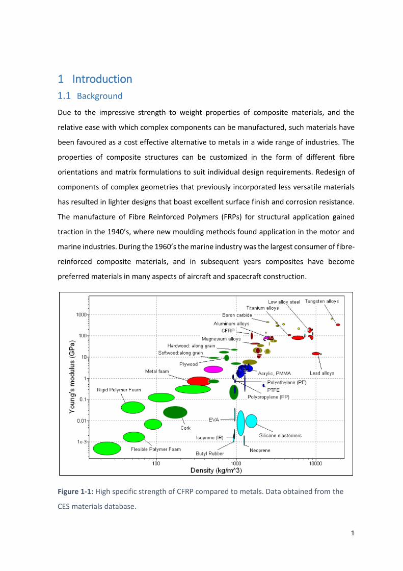
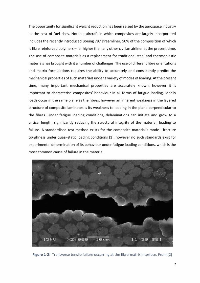


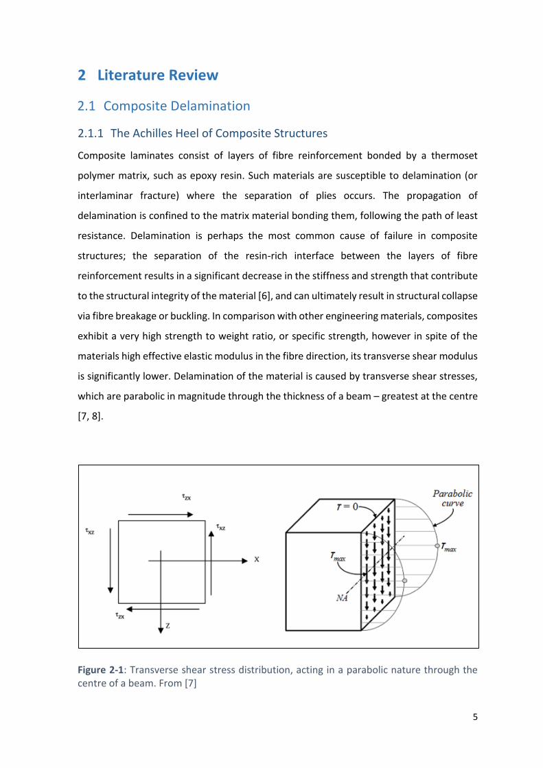
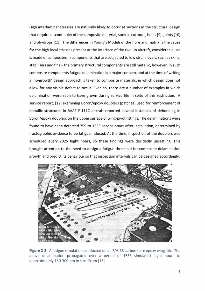
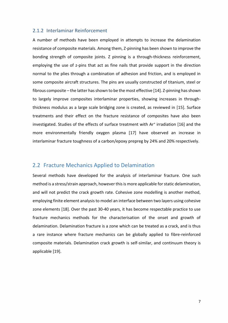
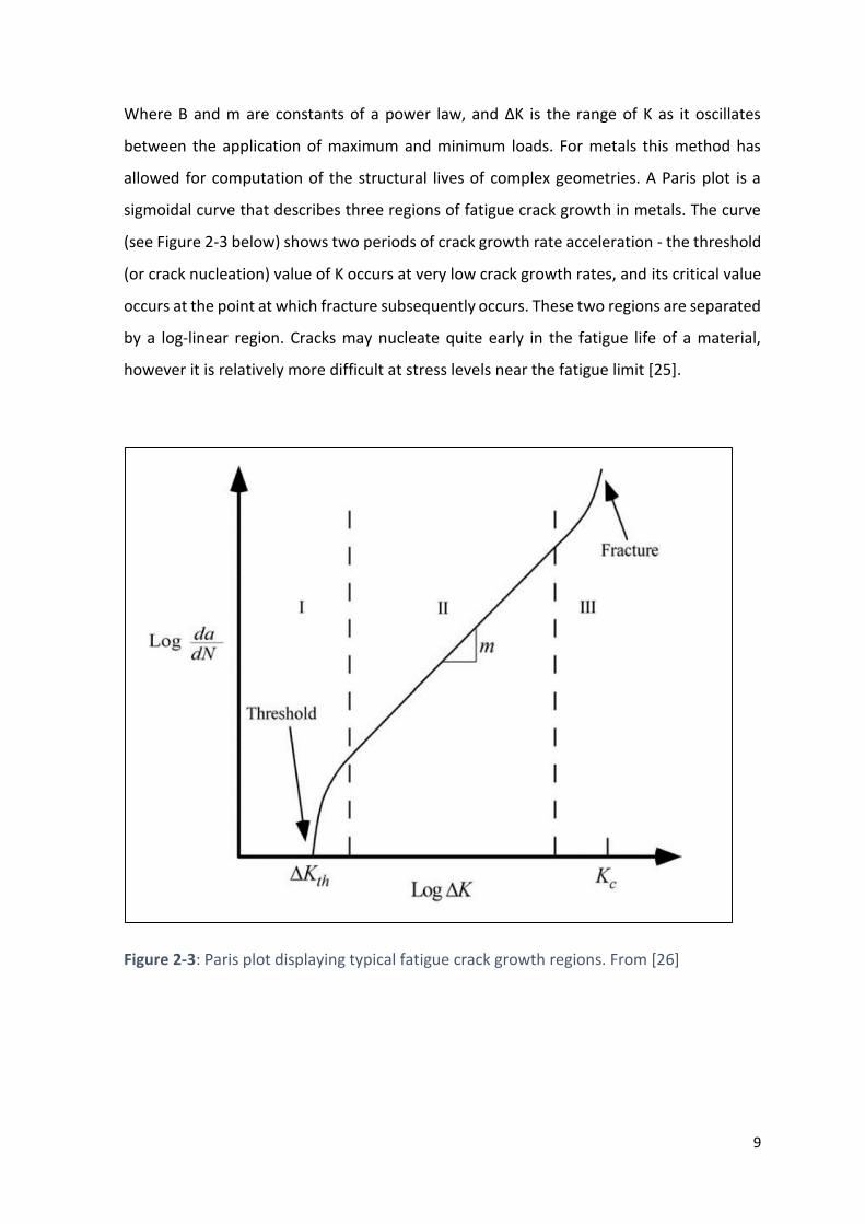

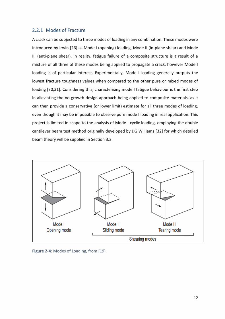

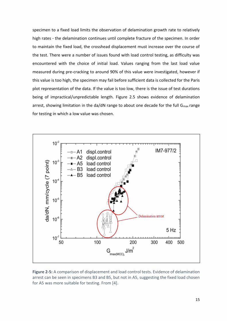
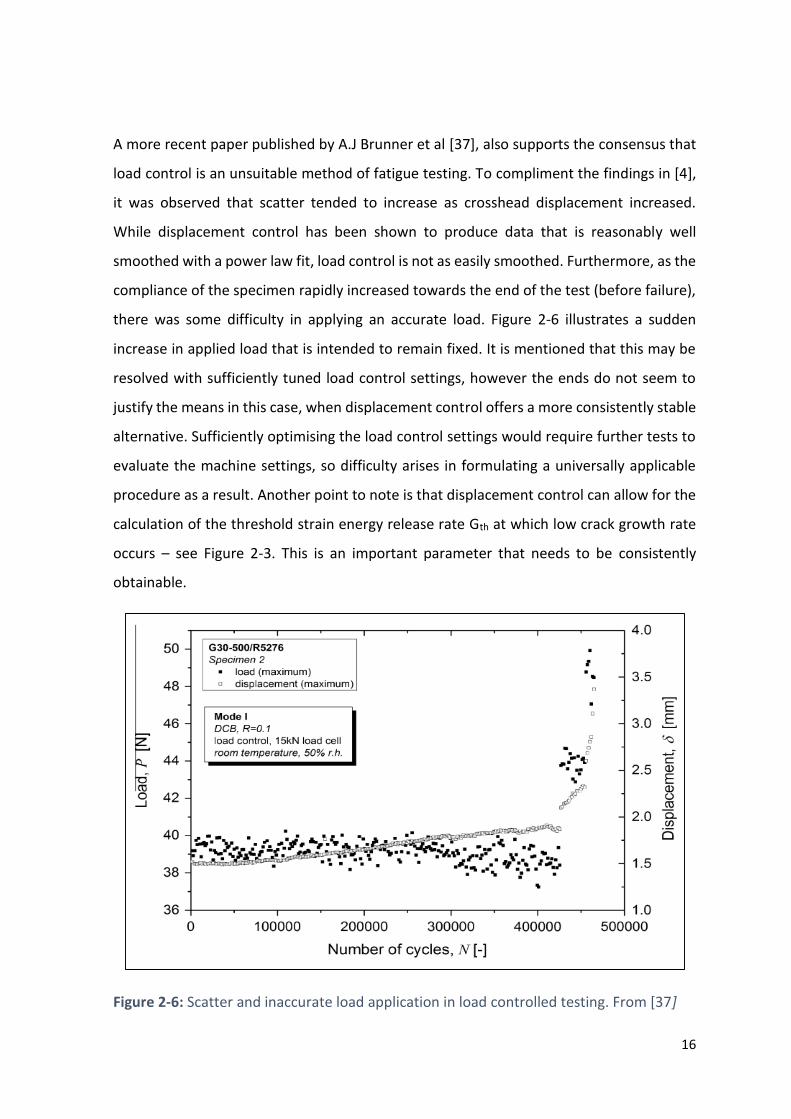
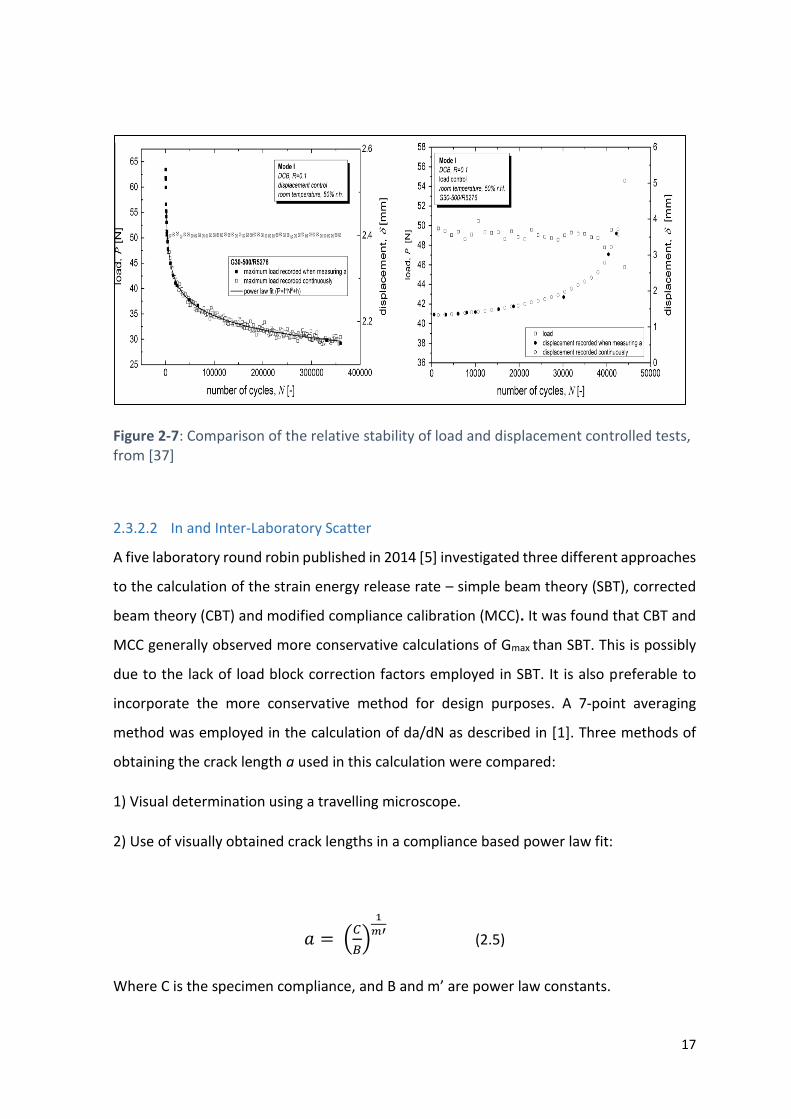
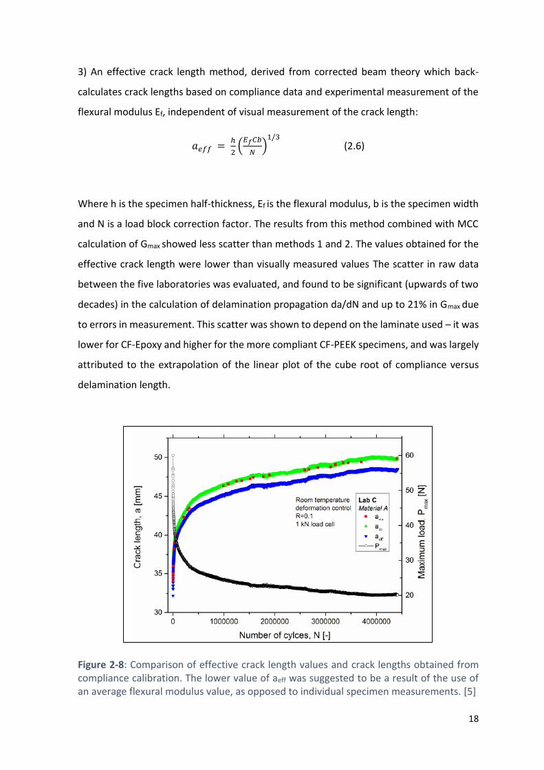
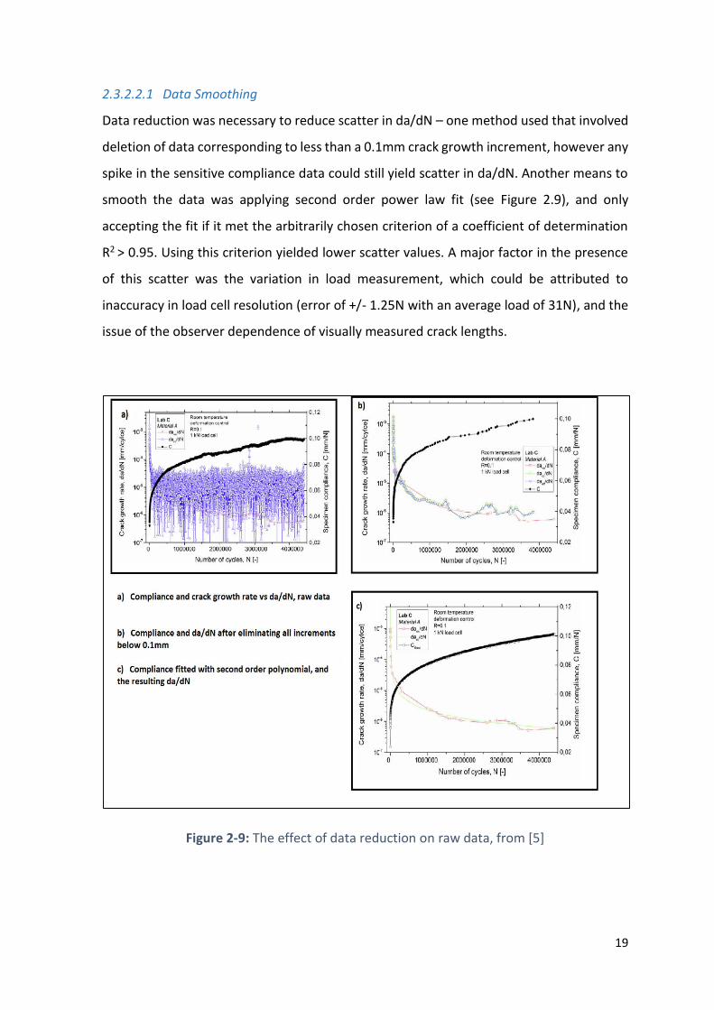

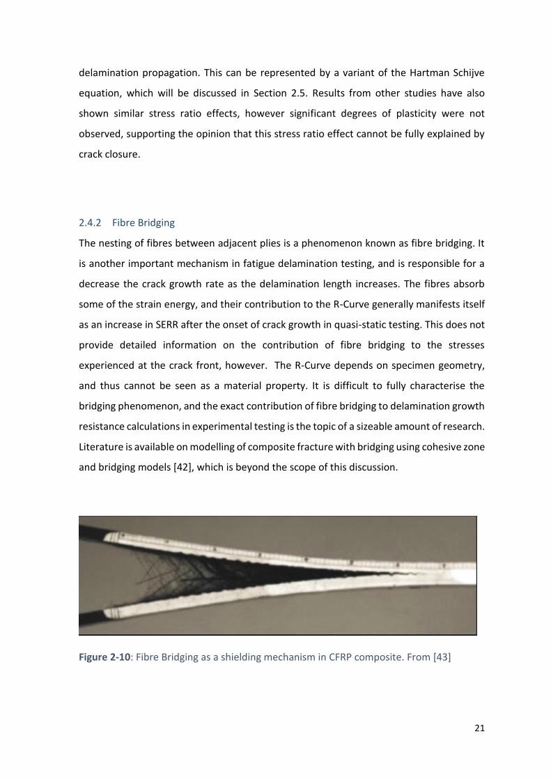
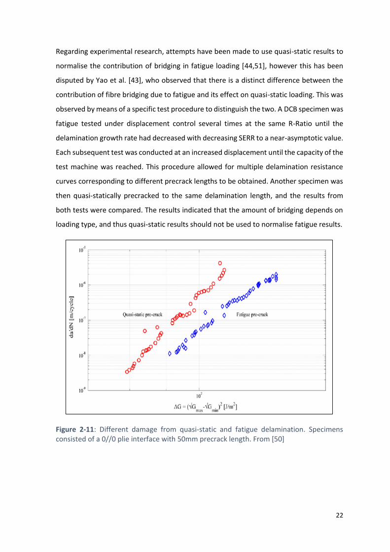

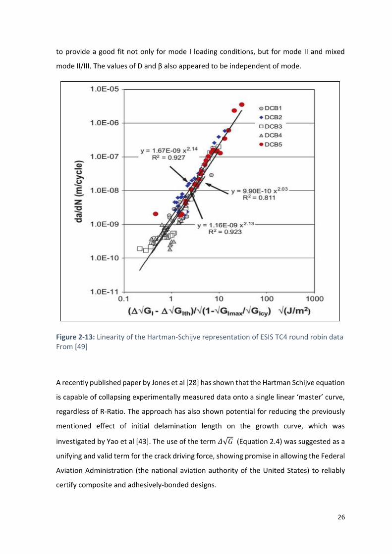


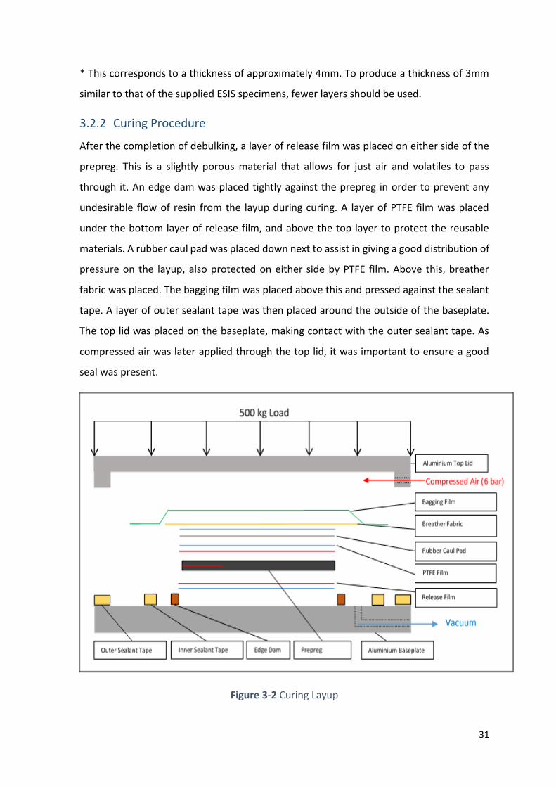

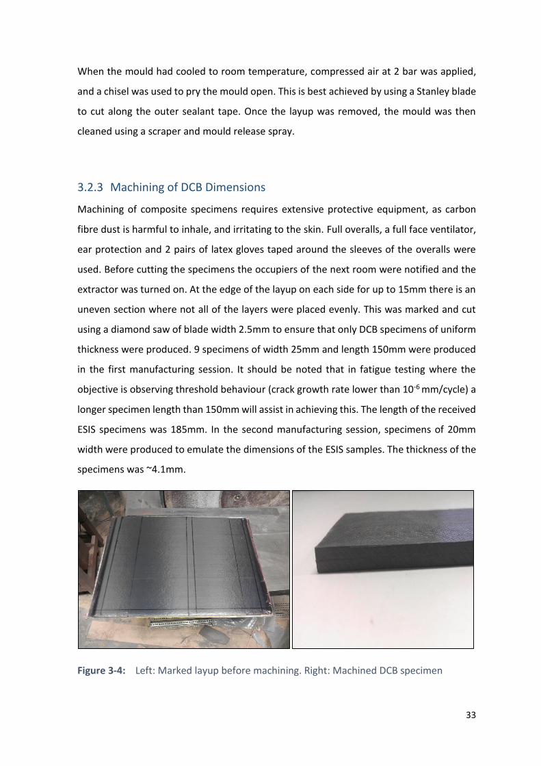


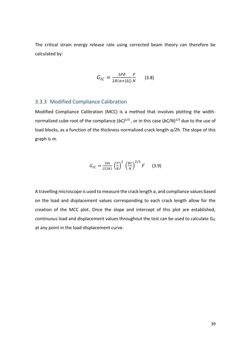

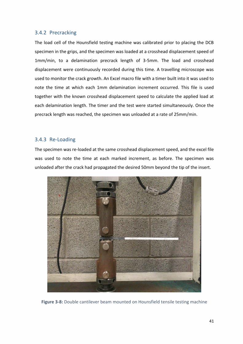

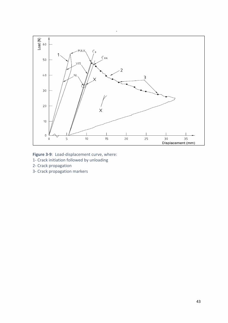
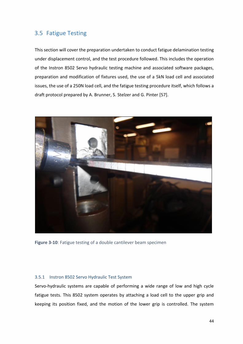


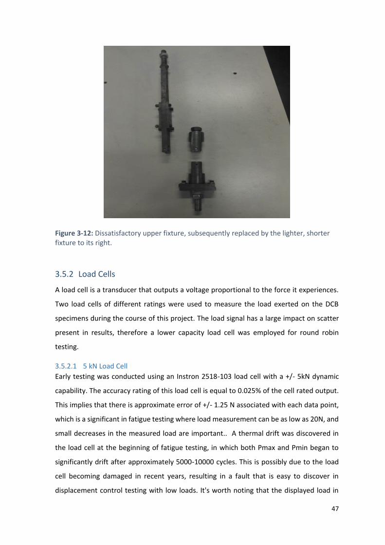

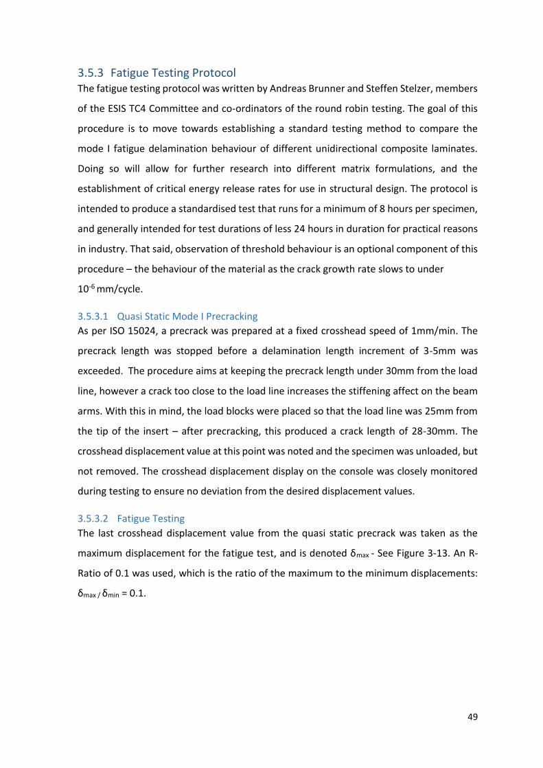
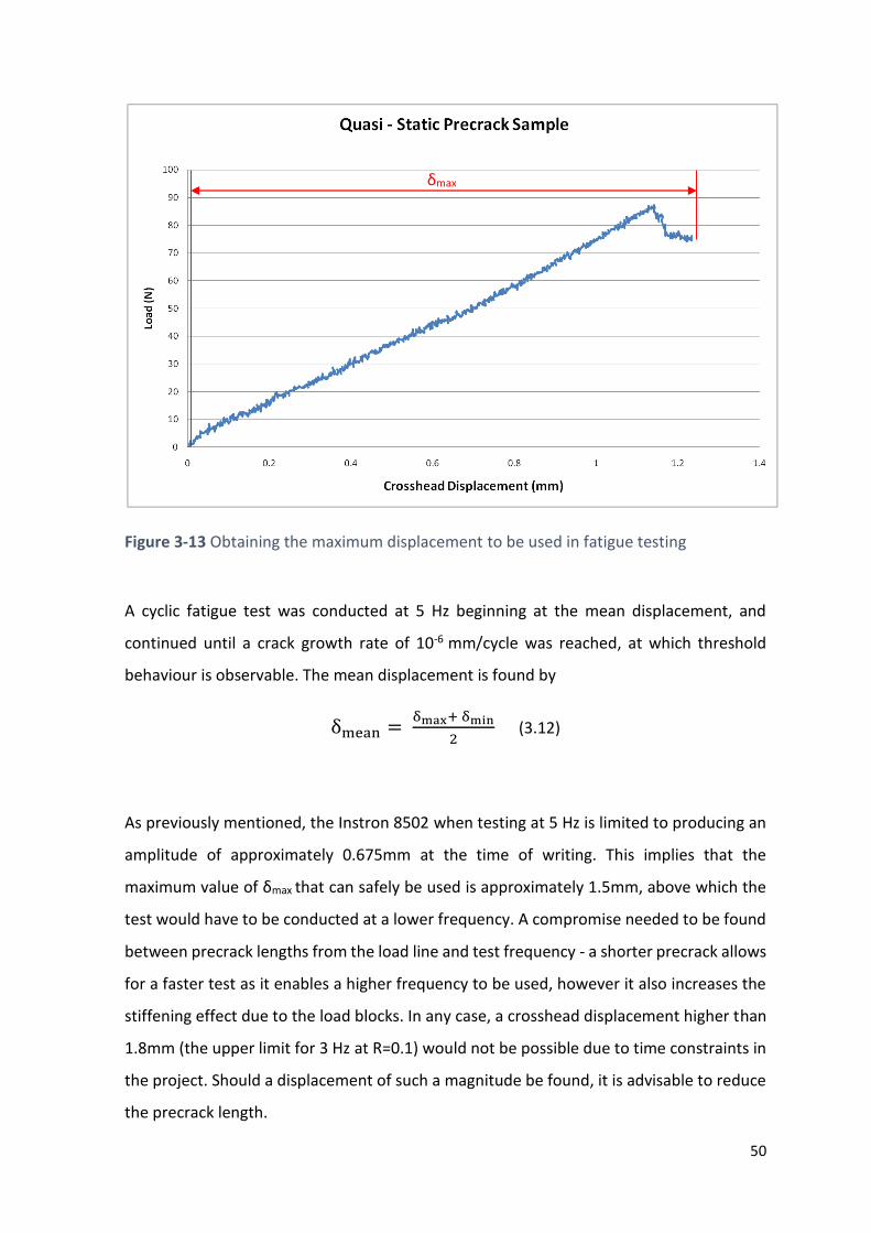
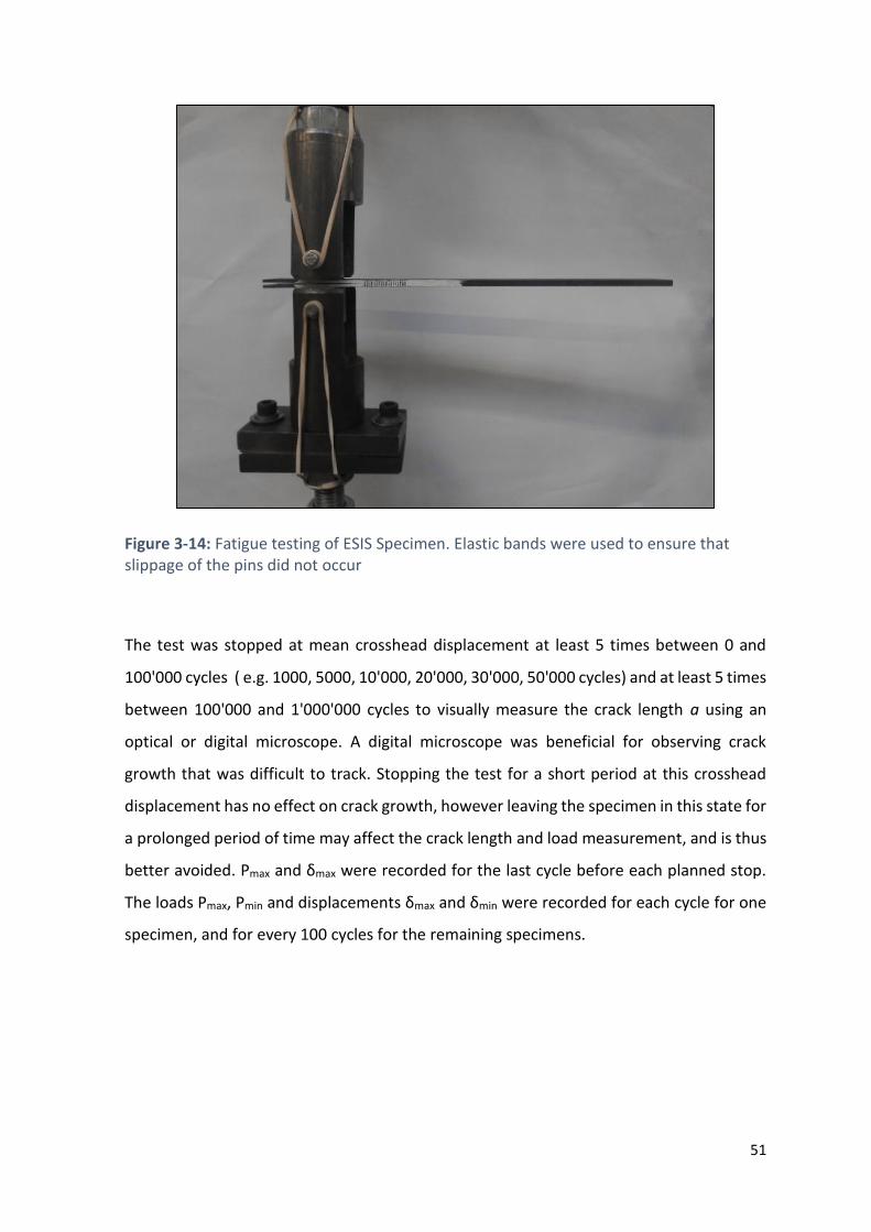


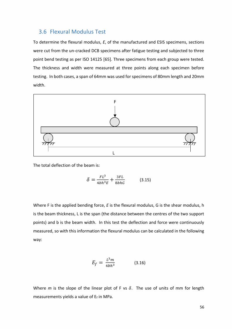

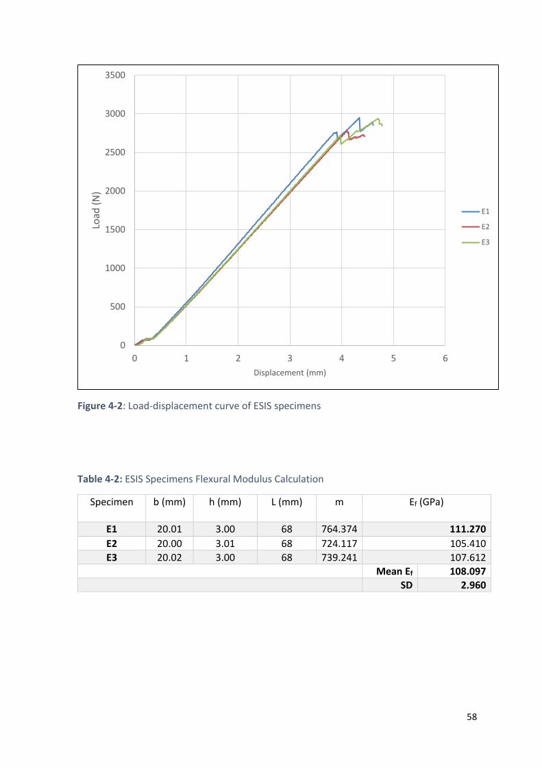
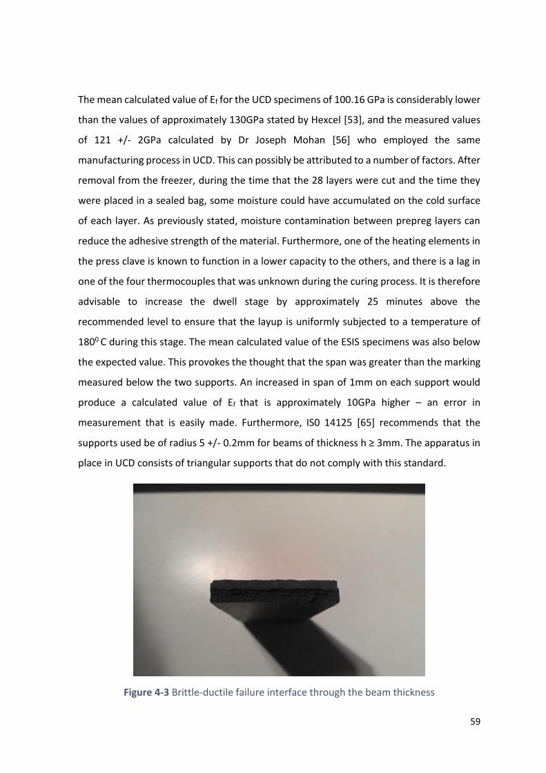


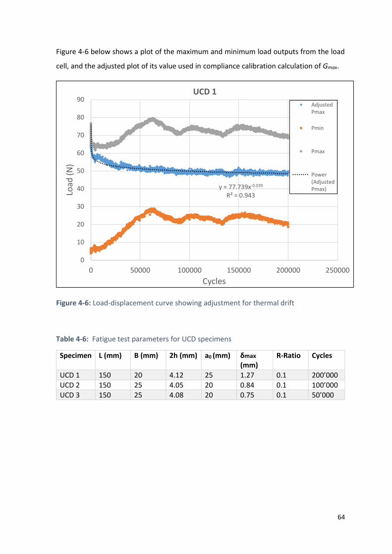


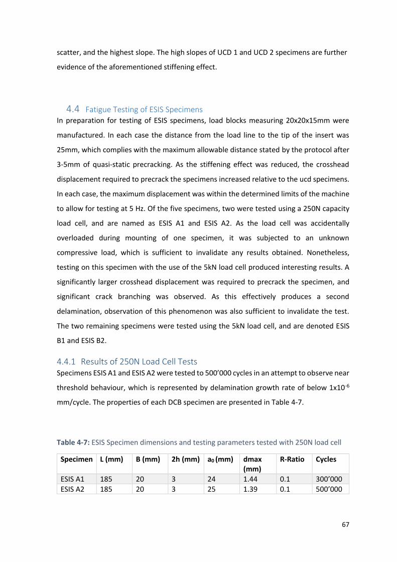
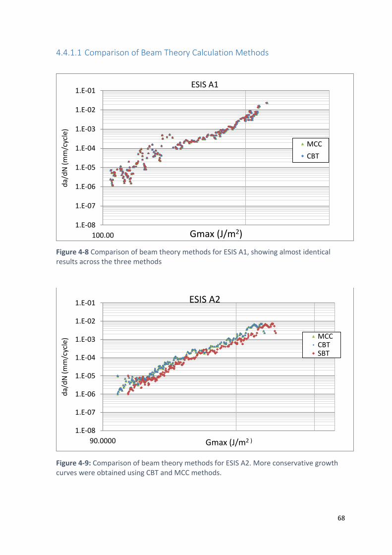
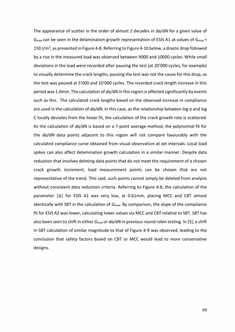
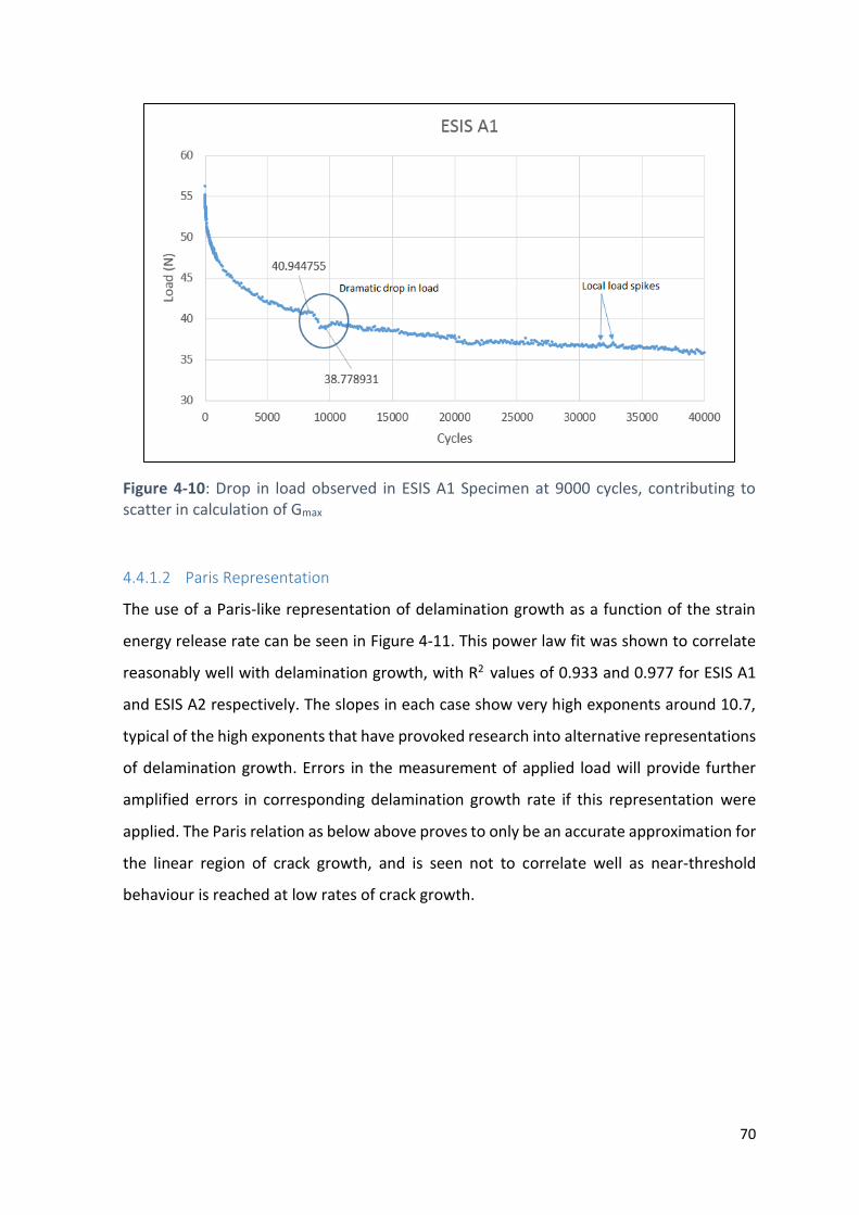
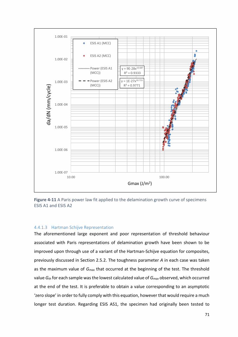
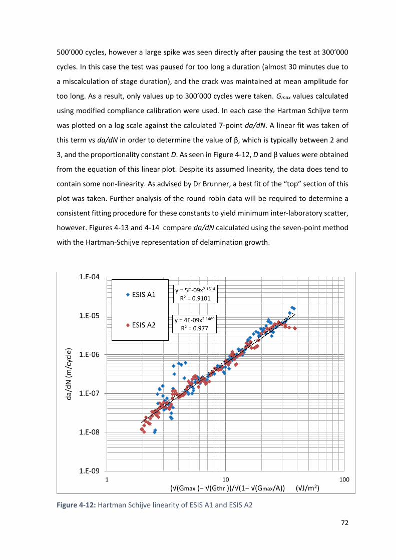

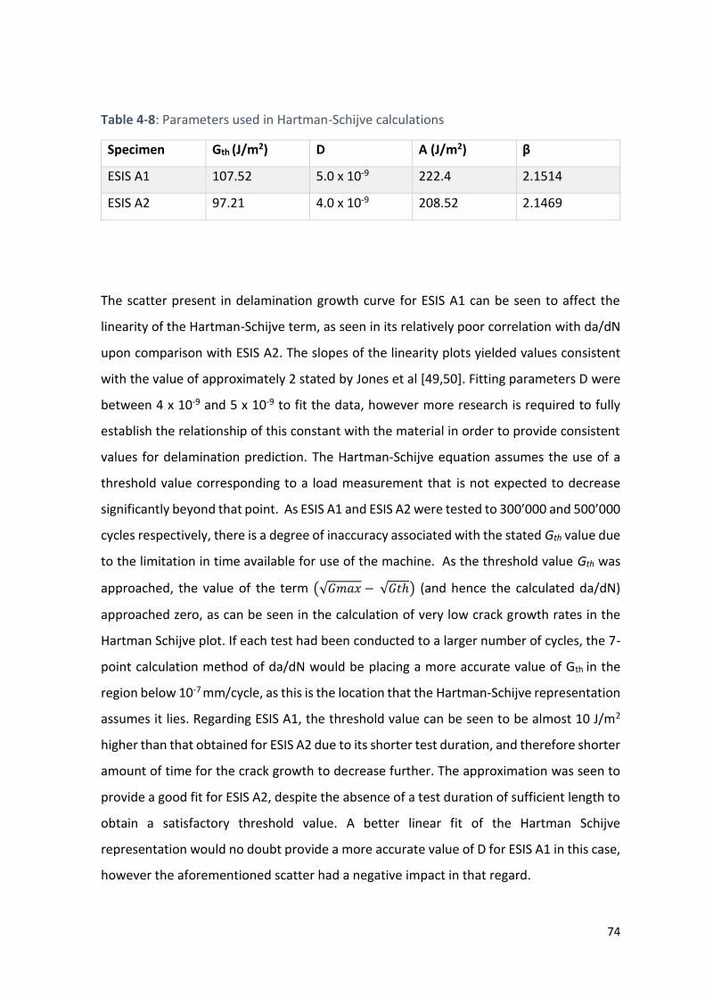
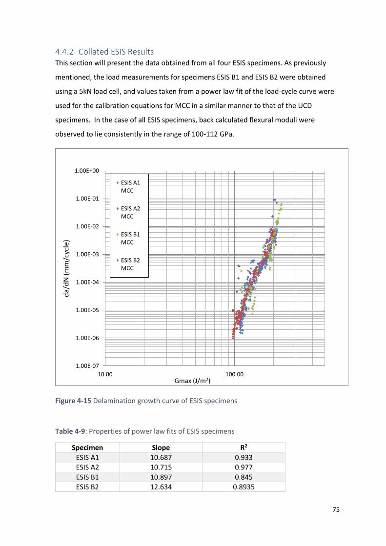


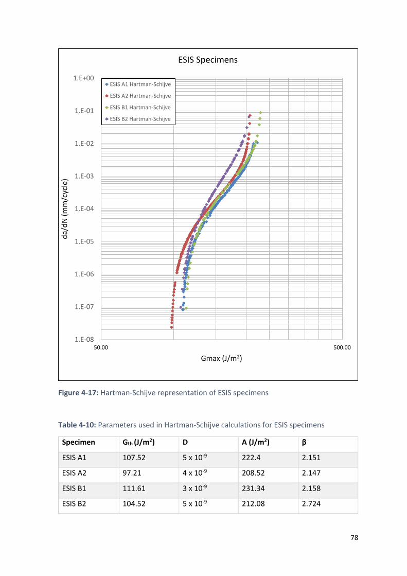
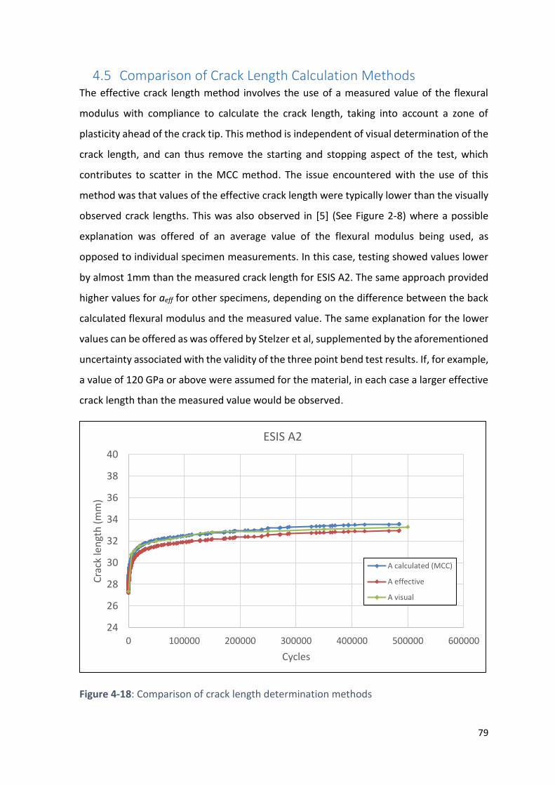
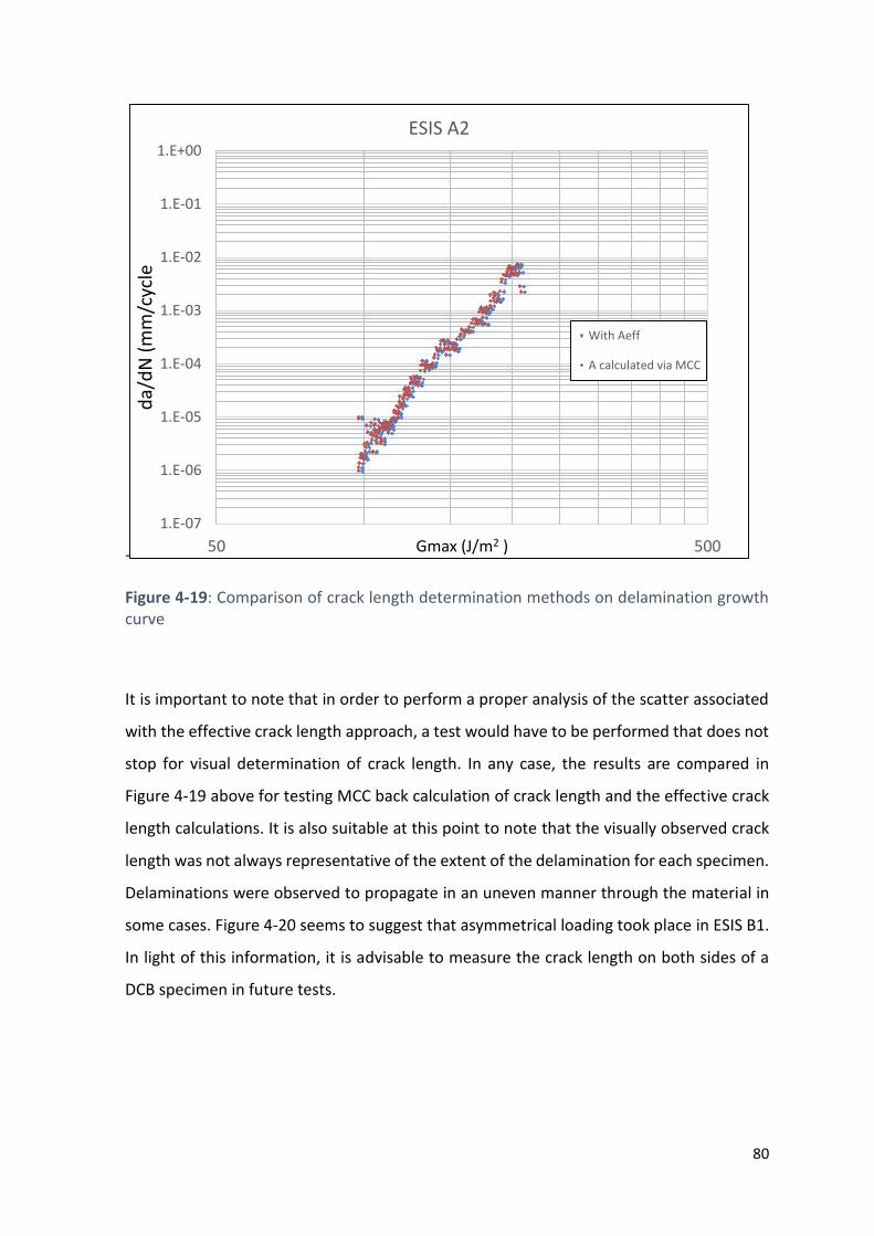

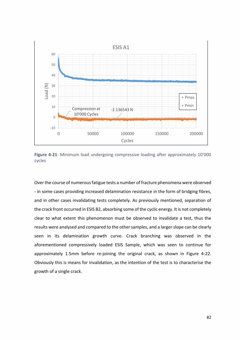


![[XLS]engineeringstudentsdata.comengineeringstudentsdata.com/downloads/2016/Telangana... · Web view2016 2016 2016 2016 2016 2016 2016 2016 2016 2016 2016 2016 2016 2016 2016 2016](https://static.documents.pub/doc/80x56/5b19478b7f8b9a23258c8745/xlseng-web-view2016-2016-2016-2016-2016-2016-2016-2016-2016-2016-2016-2016.jpg)


