Conservation risks: Whenwill rhinos be extinct?
Timothy C. Haas1 & Sam M. Ferreira2
1 Lubar School of Business, University of Wisconsin-Milwaukee, Milwaukee, USA
2 Scientific Services, SANParks, Skukuza, South Africa
Abstract
Development of driver-based scenarios of species extinction risks is in its infancy. For
many species, the dynamics of anthropogenic impacts driven by economic as well as non-
economic values of associated wildlife products along with their ecological stressors can
help meaningfully predict extinction risks. Rhinos epitomize these challenges with a key
question: When will rhinos be extinct? Extinction is complete conservation failure, collapse
of traditional Asian medicinal use, loss of income to non-government organizations, and
short-term profit for illegal traders. For rhinos, extinction is in the control of humans. We
develop an agent-based economic-ecological model that captures these effects and apply it
to the case of South African rhinos. Our model use observed rhino dynamics and poaching
statistics. It seeks to predict rhino extinction under the present scenario. This scenario
has no legal horn trade, but allows live African rhino trade and legal hunting. In addition,
rhinos have high ecotourism value and stimulate a vibrant South African wildlife industry.
Rising Asian demand for horn associates with economic well being of eastern countries.
Rising demand also introduces lengthy demand reduction strategy lag effects. Present
rhino populations are small and threatened by a rising onslaught of poaching. This present
scenario and associated dynamics predicts continued decline in rhino population size with
accelerated extinction risks of rhinos by 2036. Our model supports the computation of
extinction risks at any future time point. This capability can be used to evaluate the
effectiveness of proposed conservation strategies at reducing a species’ extinction risk.
Acknowledgement: Travel for Timothy C. Haas was supported by a SANParks Visiting
Scholar grant.
keywords: Wildlife trafficking, extinction risk, agent based economic models, ecological
modeling, individual based models
I. INTRODUCTION
The extinction of species carry several risks to society [1]. Biological diversity provides
numerous services to humans [1], most of these non-tangible and hard to quantify [1].
Conservationists, thus seek to minimize extinction risks because biological diversity provides
ecosystem resilience [2], and human quality of livelihoods associate with system resilience
1
[3]. The material value basis of most socio-economic-ecological systems [4], however, reduces
conservation outcomes to a basic price judgment. If a species pays, it stays [5].
Wildlife trafficking of charismatic mammal products, fueled by Asian demand, poses sig-
nificant threats to biodiversity persistence. International trade bans may result in poaching-
fed illegal supply chains because high demand and low supply stimulate high commodity
prices attractive to organized crime [6]. Some conservationists argue that the reliance of a
species’ persistence on its economic value is the basis of its recovery from near extinction
(e.g. the Vicuna [7]).
Rhinos are facing extinction risks [8], largely because rhino horn is of high value to
Asian societies for several cultural reasons [9], [10, ch. 14]. All rhino species’ populations
dramatically collapsed over the past century [11] with seven extant species and sub-species
remaining [12]. Asian rhino species are holding on – barely [8], while some African species
have recovered, most noticeable those with primary ranges in southern Africa [12]. Sus-
tainable use proponents argue that recognition of most values of southern white rhinos
(Ceratotherium simum simum) and to some extent southeastern (Diceros bicornis minor)
and southwestern black rhino (D. b. bicornis) is the reason for recovery [13]. Unprecedented
poaching [14] now places the continued recovery of these species at risk.
Reducing the demand for rhino horn [15], protecting rhinos better [16] and providing
horn to consumers [17] offer strategic options to combat rhino poaching. Promoters of
introducing trade in rhino horn [6], [18] relies strongly on the dependence of a species’
existence relating to its economic value. The focal mechanism, however, is a form of central
selling organization [6]. This is effectively a legal monopoly replacing or competing with
an illegal one. Cost-benefit analyses illustrate strategies that stockpile horn, provides best
financial return when the species go extinct [19], [17], [20].
Proponents of trade bans recognize non-tangible commodity values [21] and advocate
demand reduction [22] along with intensified anti-poaching tactics [16]. Trade-banners
accidentally and unknowingly trade in extinction anxiety, the key source of non-government
organization (NGO) funding. Cost-benefit analyses predict that unintended extinction
anxiety trade provides best financial return when a species remains highly endangered.
The bankers (legal and illegal stockpile traders) and betters (inadvertent extinction anxiety
traders) thus challenge the reliance of a species’ persistence on its economic value.
When will rhinos be extinct? It is not a trivial question. For conservationists, extinction
is complete failure. For Asian users, extinction collapses a medicinal tradition. For betters,
extinction degrades income. For bankers, extinction is profitable. For rhinos, extinction is
an option in the control of humans. It is within this context that we seek to predict rhino
extinction risk and when that may realize.
At present, no legal trade in rhino horn is allowed [23], but trade in live African rhinos,
part of which feed the hunting industry [5] is legal. Rhinos also contribute significantly
2
to ecotourism revenue [24] and has stimulated a vibrant wildlife industry in South Africa
[25]. Asian demand is rising [26] and associates with the ebb and flow of economic well
being of eastern countries [27]. In the short to medium term it is expected that Asian
demand for rhino horn may increase [27], [26], introducing lengthy lag effects of demand
reduction strategies. Rhino populations are relatively small and it is debatable whether
the present conservation asset can provide for the demand of rhino horn [27] even if horn is
harvested from live rhinos [6]. The present status quo is characterized by a rising onslaught
of poaching on rhinos [14].
We develop an economic-ecological model of the interaction of poachers, their mid-
dlemen, legal traders, consumers, and the South African rhino population. We integrate
an agent-based economics submodel with an individual-based rhino population model im-
pacted by the actions of the economics submodel. To the best of our knowledge, our model
is one of the first to achieve such integration. The stochasticity of our model allows us
to compute species extinction risk as the expected value of a loss function where “loss” is
defined to be the non-use value of rhinos residing in a protected area [28].
This article is structured as follows. In Section II, we describe the current situation
surrounding rhino horn trade and consequent rhino poaching. Then, in Section III, we
describe our economic-ecological model of this trade and its impact on the South African
white rhino population. In Section IV, we predict extinction risks over a 35 year hori-
zon. In Section V, we compare our model’s output to data-based estimates of white rhino
abundance and generate predictions of the coupled dynamics of rhino horn trade and rhino
abundance. We discuss the implications of our results in Section VI and reach conclusions
in Section VII.
II. SUPPLY AND DEMAND OF WILDLIFE PROD-
UCTS
Bulte and Damania [29] employ an economic model to find that multiple equilibrium states
exist when a legal trade system operates in parallel to an illegal one. Some of these equi-
librium states exhibit accelerated poaching leading to the extinction of the species being
harvested. These are called Bertrand equilibrium states. The opposite of Bertrand equilib-
rium is Cournot equilibrium wherein the higher-priced trader’s market share is reduced.
Ferrier [30] derives equilibrium models of the size of price differentials needed for illegal
wildlife trafficking to take place. These models refer to the situation wherein a country
has issued a trade ban that makes it illegal to harvest a wildlife product in that country.
Ferrier [30] also models the effects of the smugglers’ level of risk aversion, the probability
that a smuggler will be caught and penalized, and the price elasticity of demand for the
wildlife product.
3
The definition of price elasticity of demand is the percentage change in quantity de-
manded divided by the percentage change in price [31]. It has been observed that doubling
rhino horn price has little to no effect on the demand for it [32]. In other words, the demand
for rhino horn is inelastic. There is some evidence [27], [33] that the demand for rhino horn
is about four times the amount that is actually sold. Hence, it is important to distinguish
between what the total demand for rhino horn is versus the portion of that demand that
is satisfied.
A. Competition
We consider three products traded in three largely separate markets: (1) horn for Asian
consumers, (2) live rhinos for the South African recreational hunter market, and (3) the
international market for satisfying global anxiety about the future of biodiversity. We refer
to the third market as the Species Extinction Anxiety Reduction (SEAR) market.
The last market is served by private firms and NGOs, hereafter referred to as simply
SEAR traders. It is in the interest of SEAR traders to amplify and keep in the media
the idea that the rhino is headed for extinction due to poaching. In other words, if rhinos
cease to be endangered, the global feeling of anxiety towards the future of rhinos would
be reduced thus reducing the demand for the service SEAR traders are selling (anxiety
reduction).
There are three consumer groups: horn consumers in Asia, donors to SEAR traders,
and recreational hunters of rhinos. There is little overlap between these groups. Legal and
illegal traders would engage in direct competition if consumers of rhino horn were able to
choose between illegal and legal horn.
B. The Nature of the Illegal Rhino Horn Trade
Illegal traders have bribery costs but no supply maintenance costs, no taxes, no regulation
costs, and no labor union costs. Generally then, their overhead costs can be lower than
legal traders. And they do not reinvest any of their profits in growing or maintaining
their supply so that their profit margins can be larger than that of a legal trader [34].
Crime syndicates pay a small sum [35] to poor, rural people who have limited economic
opportunities [36] thus almost guaranteeing an illegal supply of rhino horn.
In a review and critique of the literature on the coexistence of legal and illegal rhino
horn trade, Campbell [37] does not find compelling arguments or evidence pointing towards
a legal rhino horn trading scheme driving illegal rhino horn traders out of business. There is
some reason to believe that competition may actually increase poaching (e.g. [29]). Due to
the potential complexity of side-by-side legal and illegal rhino horn markets, any economic
model of a competing legal and illegal horn trade needs to account for several elements.
4
The first is recognizing imperfect competition - organized crime continues to have a
near monopoly on tradable horn. Organized crime can thus manipulate supply in order to
force higher prices. Second, demand is so great it is mostly inelastic to supply. In addition,
poachers will conduct poaching raids for very small wages because there are almost no other
competing labor sectors open to them. Therefore, as long as the criminal network can sell
horn, they will most likely continue to sponsor poaching raids. The reality is that criminal
networks have few rules. In contrast, legal traders have maintenance costs and transaction
costs that are substantially higher than what illegal traders have.
III. THE ECONOMIC-ECOLOGICAL MODEL
Source code for the economic-ecological model (available at [38]) captures a model that con-
sists of two interacting, stochastic submodels: an agent-based model of competing traders
modified from a model developed by Catullo [39], and an Individual Based Model (IBM)
[40] of a wildlife population modified from a model developed by Kostova, Carlsen, and
Kercher [41].
A. Applying Agent-Based Economic Models to Wildlife Trade
An agent-based economic model represents individual firms as agents and individual con-
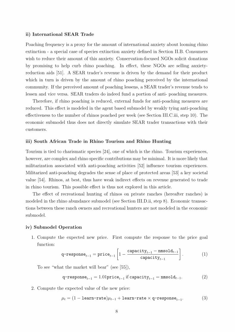
sumers as agents. During one step or cycle, each trader makes decisions about product
re-supply and product pricing that maximizes their individual utility. Also during this cy-
cle, each consumer makes decisions about entering a market, and once entered, purchasing
decisions that maximize their individual utility. Time is incremented, and another cycle is
executed [42], [43], [44].
Building on Catullo [39], we construct an agent-based submodel of the international
trade in rhino poaching goods across three markets. Our submodel contains a criminal
network involved in illegal rhino horn trafficking, a firm involved in seeking to trade legally
in horn, the effect of a meta-firm serving the international SEAR market, and the effect of
a local, South African meta-firm serving the rhino hunting market.
Arthur [45] finds that an agent-based economics model is able to distinguish among
multiple equilibria: a feat that is difficult for models formed from the equilibrium solutions
of systems of differential equations. The suspected existence of multiple equilibria in the
dynamics of wildlife products trade [29] is possibly the central reason for the reluctance
that non-government organizations and international convention secretariats such as CITES
have towards the legalization of trade in wildlife products from endangered species. In
essence, these agencies suspect multiple equilibria and have no assurance that reality will
not settle into an equilibrium point of a species’ extinction.
Arthur [45] also notes that agent-based economics models can model the effect that
5
trader expectations can have on future product supply. An example of this in the present
application is where illegal rhino horn traders expect to be undersold once legal horn trading
is enacted - leading them to accelerate their poaching activities to maximize their profits
before being forced out of the market [19].
In another review and critique of the literature advocating legal trade in wildlife prod-
ucts [46], the authors find many articles reaching conclusions based on analyses of static
models. The authors see this as inadequate as such models cannot shed light on how
wildlife trade markets might unfold through time. Our agent-based submodel on the other
hand, is a fully dynamic approach. The authors are also critical of the assumption of a
downward sloping demand curve present in all pro-trade articles. Recent theoretical results,
specifically the Sonnenschein-Mantel-Debreu theorems (see [46] have shown that a market
demand curve need not share any characteristics of an individual’s demand curve. Hence,
any theory that assumes aggregate behavior is a simple scaled function of individual be-
havior is theoretically invalid. Again, our agent-based submodel allows aggregate behavior
to emerge from the interacting actions of many individual consumers.
B. Integrating Economic Behavior and Wildlife Dynamics
In our approach, an IBM [41] is employed to represent the South African rhino population
as they are impacted through time by their birth process, natural death process, and the
poaching process produced by the agent-based economics submodel of the legal and illegal
traders (Fig 1).
In this model, the traders’ submodel runs every 12 weeks and produces m, the number
of rhinos to poach each week for the next 12 weeks. Then, the rhino IBM runs every week
for 12 weeks. Each week, m mature rhinos are randomly selected and set to the value dead.
C. Traders as Agents
Note that in the present state of rules, legal rhino horn traders are only seeking to obtain
permission to trade, but are not trading any rhino horn.
i) Rhino horn traders
In our economic submodel, there are two traders, one legal and one illegal. There are
several levels of middlemen involved in the illegal rhino horn trade [47]. We model these
as one meta-firm, i.e., we model the middlemen that directly purchase rhino horns from
poachers up through the exporters as working for a single firm: the illegal trader. We
argue that a criminal middleman has a restricted number of potential customers: other
criminal middlemen or criminal exporters. Hence, the collection of middlemen up through
the exporter acts more like a cooperative than a set of competing firms. Implicit profit
6
sharing occurs as a middleman at one level will only be willing to purchase rhino horn from
a lower level middleman if that price allows the middleman to make a profit. Ultimately,
the ability of this cooperative to make a profit depends on the price demanded by poachers
and the black market price that consumers are willing to pay. As long as the unit cost to
this cooperative is lower than consumers’ reserve price, the illegal trader will stay in the
business of rhino horn trafficking – lowering or raising their black market price in response
solely to the purchase decision making of consumers. Therefore, some estimate of an illegal
trader’s unit cost is needed.
In our economic submodel, the unit cost for acquiring and selling one kilogram (kg) of
rhino horn by either trader is $5,000. For the illegal trader, this number is arrived at by
considering that trader’s costs as follows. First, the illegal trader needs to purchase a horn
from a poacher. In Eloff and Lemieux [48, p. 21], the black market price for one kilogram
of rhino horn is estimated to be between USD $35,000 and $60,000 with about 5% of that
being used by the illegal trader to purchase the rhino horn from poachers. Using the lowest
black market price, poachers are paid $1,750 for one kilogram of rhino horn. Next, the
illegal trader needs to purchase a courier’s airfare from Maputo, Mozambique to some city
in Asia for $2,000. Finally, the illegal trader needs to pay the courier’s fee of $500 [49]
per rhino horn or $100 per kilogram of rhino horn assuming an average rhino horn weighs
about 5kg [50]. Using these numbers, the trader has incurred a cost of $3,850 to bring one
kilogram of rhino horn to an Asian market. Thus, a conservative unit cost is $5000.
As mentioned in Section II, the literature speculates that the legal and illegal traders
may settle into an equilibrium state wherein the illegal trader pays to accelerate the poach-
ing rate. Our model is constructed so that either trader will continue to produce their
product (through poaching for the illegal trader) as long as their unit cost is less than
what they can sell the product for. Therefore, our model’s output (not shown) has the
two competing traders settling into an equilibrium state wherein the traders both quickly
drop their prices to their respective unit costs. If one trader’s unit cost is higher than the
other’s, that trader is driven out of the market. This is not Bertrand equilibrium because
neither trader is strategically over-producing. And it is not Cournot equilibrium either
because neither trader is voluntarily offering fewer products for sale.
Traders are not allowed to engage in product “dumping,” i.e., sell their rhino horns for
less than their unit costs. Each week, traders always sell as many kilograms of rhino horns
as there are consumers willing to purchase them. In other words, demand is insatiable [27].
Vietnamese rhino horn merchants usually have a number of rhino horns available for
inspection [34]. This implies that (a) there is no direct order placed by a customer before a
rhino is poached, and (b) illegal traders maintain a buffer stock (inventory) of rhino horn.
7
ii) International SEAR Trade
Poaching frequency is a proxy for the amount of international anxiety about looming rhino
extinction - a special case of species extinction anxiety defined in Section II.B. Consumers
wish to reduce their amount of this anxiety. Conservation-focused NGOs solicit donations
by promising to help curb rhino poaching. In effect, these NGOs are selling anxiety-
reduction aids [51]. A SEAR trader’s revenue is driven by the demand for their product
which in turn is driven by the amount of rhino poaching perceived by the international
community. If the perceived amount of poaching lessens, a SEAR trader’s revenue tends to
lessen and vice versa. SEAR traders do indeed fund a portion of anti- poaching measures.
Therefore, if rhino poaching is reduced, external funds for anti-poaching measures are
reduced. This effect is modeled in the agent based submodel by weakly tying anti-poaching
effectiveness to the number of rhinos poached per week (see Section III.C.iii, step 10). The
economic submodel thus does not directly simulate SEAR trader transactions with their
customers.
iii) South African Trade in Rhino Tourism and Rhino Hunting
Tourism is tied to charismatic species [24], one of which is the rhino. Tourism experiences,
however, are complex and rhino specific contributions may be minimal. It is more likely that
militarization associated with anti-poaching activities [52] influence tourism experiences.
Militarized anti-poaching degrades the sense of place of protected areas [53] a key societal
value [54]. Rhinos, at best, thus have weak indirect effects on revenue generated to trade
in rhino tourism. This possible effect is thus not explored in this article.
The effect of recreational hunting of rhinos on private ranches (hereafter ranches) is
modeled in the rhino abundance submodel (see Section III.D.ii, step 8). Economic transac-
tions between these ranch owners and recreational hunters are not modeled in the economic
submodel.
iv) Submodel Operation
1. Compute the expected new price. First compute the response to the price goal
function:
q-responset−1 = pricet−1
[1−
capacityt−1 − nmsoldt−1
capacityt−1
]. (1)
To see “what the market will bear” (see [55]),
q-responset−1 = 1.01pricet−1 if capacityt−1 = nmsoldt−1. (2)
2. Compute the expected value of the new price:
µt = (1− learn-rate)µt−1 + learn-rate× q-responset−1. (3)
8
3. The new price is found by sampling once from a normal distribution with mean µt
and a standard deviation of $200.
4. The net revenue is:
netrevt = nmsoldt−1(pricet−1 − unit-cost). (4)
5. The response to the production capacity goal function is:
c-responset = netrevt − netrevt−1. (5)
6. The production capacity decision constant is:
q-prodcapt = (1− learn-rate)q-prodcapt−1 + learn-rate× c-responset. (6)
7. The production capacity decision Binomial distribution probability is:
pc =q-prodcapt + maxnetrev
2× maxnetrev. (7)
8. Production capacity is reduced, left unchanged, or increased according to the follow-
ing rules. First, let D be a binomially distributed random variable with n = 2,
and probability of success equal to pc. Sample once from this distribution. If
d = 0, prodcapt = prodcapt−1 − 1. If d = 1, prodcapt = prodcapt−1. If d = 2,
prodcapt = prodcapt−1 + 1 up to this trader’s maximum production capacity. Both
traders have a maximum production capacity of 150kg of rhino horns per week. Be-
cause the horns from an adult rhino weigh approximately 5kg, this value represents
30 rhinos per week. In 2013, an average of 20 rhinos were poached per week across
South Africa [56]. Hence, this maximum is ten rhinos above the 2013 weekly average.
9. Reduce the production capacity of the illegal trader in proportion to the effectiveness
of anti-poaching operations as follows. Let Np be binomially distributed with n =
prodcapt and probability of success equal to pa. The probability pa is set to a number
close to 0.0 if anti-poaching operations are very effective at curbing poaching. Sample
once from this binomial distribution to find np, the actual number of rhinos poached
this week in spite of anti-poaching operations.
10. Model the effect of additional anti-poaching funds donated by SEAR traders by re-
ducing np by 5% if np is greater than 25.
11. Model the effect of population growth on the Asian continent on the number of
potential rhino horn consumers. Most consumers of rhino horn live on the Asian
continent [26]. Table 1 contains population projections found in [57].
9
The initial consumer population is created as follows. To represent the assumption
of insatiable demand at current (illegal) production levels, consumers are created as
necessary to purchase all rhino horn poached under the maximum poaching rate of
30 rhinos per week across South Africa (20 in KNP, and 10 on the ranches). Because
each rhino horn weighs on average 5kg, these numbers are multiplied by 5. Therefore,
in the year 2014, the potential number of consumers is set to 300 (5×60). This value
is increased in proportion to the entries in Table 1 to a maximum of 325 in the year
2033.
For the case of a legal trading scheme operating in parallel to the illegal trade, this
consumer pool is doubled. Because demand for rhino horn in the near future is
predicted to be about four times current sales [27], doing so is well-within current
demand forecasts. The supply of legally-traded rhino horn would be sourced from
stockpiles and/or shavings from live rhinos.
By a “consumer” we mean a group composed of a number of real-life individuals.
Guilford [58] reports an individual purchase for $2000 of rhino horn powder. At the
per-kilogram prices mentioned above, this would be between 33 and 57g of rhino
horn. Other individuals may purchase other amounts of rhino horn. In our model
however, one of our “consumers” always buys exactly one kilogram of rhino horn at
each purchase event. Hence, one of our “consumers” represents approximately 18
to 30 real-life individuals. By doing so, we ignore the variability in the amount of
purchased rhino horn and in-effect, lump approximately 18 to 30 real-life purchase
events into one purchase event. Hence, our purchase event time series shown below
should be viewed as the aggregate behavior of groups of approximately 18 to 30
real-life individuals.
12. Consumer behaviors start with the decision to enter the rhino horn market or not. If
there is a media campaign aimed at potential rhino horn consumers that delivers a
message that rhino horn has no medicinal value, some of the potential consumers may
decide to not try to purchase rhino horn. This media campaign effect is represented
as follows. Let npc be the number of potential consumers each week. Let pm be the
effectiveness of a horn-is-not-medicine media campaign run in the country where the
consumers live. If pm is close to 1.0, the chance that a randomly chosen potential
consumer will decide to buy rhino horn is close to zero. Let Nc be binomially dis-
tributed where there are npc trials, and the success probability is 1−pm. Sample once
from this distribution to find nc, the number of consumers for that week who enter
the market for rhino horn.
13. Simulate rhino horn purchases. Each consumer buys one kilogram of rhino horn from
the trader offering it at the lowest price as long as this price is below the consumer’s
10
reserve price of $60,000 [14]. Because the illegal trader maintains a buffer stock of
rhino horn, the number of kilograms of rhino horns the illegal trader sells each week
need not equal five times the number of rhino horns poached the previous week.
D. An Individual-Based Model of the Rhino Meta-Population
An IBM of animal abundance is valid for any range size and number of animals when
data structures and mapping functions are suitably developed [40, ch. 4]. But a differen-
tial equation model of the animal’s population dynamics (see [59]) may, depending on the
assumptions that underlay its derivation, need relatively larger range sizes and initial abun-
dance values for it to be a faithful representation of actual population dynamics. Within
ranches however, rhino abundance and range are often small.
An important characteristic of this habitat is that rhino are artificially restricted to
anthropogenically-defined patches which in this case are those within the subregions of
Kruger National Park (KNP) and ranches. An IBM can be developed to accurately repre-
sent the effects of these restrictions on the dynamics of the within-patch populations. The
ability of IBMs to handle complex habitat-use conditions is one reason given by McLane,
Semeniulk, McDermid, and Marceau [60] for why IBMs should be used to model managed
wildlife populations.
A spatially-explicit submodel of the South African rhino meta-population is built as
opposed to a non-spatial, aggregated single population submodel for the following reasons:
1. Different tolerances for risk across ranch owners can be modeled. For example, a
ranch owner might offer the opinion: “I won’t keep rhinos, too risky.”
2. Ranch-specific financial returns for keeping rhinos can be modeled.
3. Spatial effects on the amount of available forage can be modeled.
4. Spatially-heterogeneous anti-poaching effectiveness can be modeled.
5. Spatially-heterogeneous poaching pressure can be modeled.
6. Rhinos are highly territorial [61]. A spatially-explicit IBM is flexible enough to real-
istically capture all aspects of this behavior.
An IBM for the South African rhino meta-population is developed along the lines of
the prairie vole (Microtus ochrogaster) IBM of Kostova, Carlsen, and Kerche [41]. As with
the prairie vole IBM of [41], the rhino IBM is stochastic in that one run over a time period
will not necessarily produce the same history of abundance and dispersal as another run
over the same time period. For this reason, many replications of the IBM over the same
time period are needed so that at each time point, both the expected value of abundance
and extinction probability can be computed.
11
i) Rainfall Predictions and Available Vegetation
Rainfall predictions for KNP over the simulation interval (Figure 2) are found by evaluating
a mathematical model that has been statistically fitted to rainfall observations. Rainfall
data from the years 1903 through 2013 contained in the SANParks data repository [62] are
used to estimate the parameters of a neural network time series model that includes the
effect of the El-Nino-Southern Oscillation (ENSO) phenomenon [63]. A logistic transform
[64] to a quasi-periodic function formed from the product of three cosine functions [65] is
used to model the ENSO phenomenon.
The rainfall predictor at time t is constructed as follows.
1. The quasi-periodic function is
qt =3∏
i=1
cos
[πt− ϕ
γi
], i = 1, . . . , 3 (8)
where ϕ is the phase, γi is the period of the ith component, and ζ is the amplitude.
2. The logistic function is:
mt = [1 + exp(−β(ζqt − α))]−1 . (9)
3. A neural network nonlinearly transforms mt to produce a rainfall prediction:
hti = (1+exp(−ω1iyeart−ω2iweekt−ω3iweeknmt−ω4imt−ω5i))−1, i = 1, . . . , nh (10)
where nh is the number of “hidden rows” in the neural network, weekt is the week
counter starting at week 1 in the year 1903, and weeknmt is the number of the week
within the year and takes on the values 1, . . . , 52. The neural network’s output layer
consists of a single variable:
ot =
[1 + exp
(νnh+1 +
nh∑i=1
νihti
)]−1
. (11)
The parameters of this model are ϕ, γ1, γ2, γ3, β, ζ, ωij, i = 1, . . . , 5, j = 1, . . . , nh, and
νi, 1, . . . , nh+1. Least squares parameter estimates are found with nonlinear optimization.
Rainfall either observed or predicted is used as a scaled proxy of available vegetation.
A scaling constant is selected so that approximately 25% of the population experiences a
food deficit during the dry season [66].
Specifically, a value of c is found such that
0.75 =c× a× v
12000× wfi(12)
12
where a is the area of KNP, v is unscaled available vegetation for week i set equal to the
0.91 quantile of the observed rainfall observations from 1910 to 2012, and 12, 000 is the
desired (target) value of rhino abundance in KNP. Week i’s new vegetation per square
kilometer is computed from the week i’s rainfall with vegi = c× ri where i = 1, . . . ,m and
m is the number of weeks in the observation or prediction interval.
At any point in time, the available vegetation for a rhino’s food supply is no more
than 36 weeks old. To model this, the net vegetation in a week is set to the sum of the
left-over vegetation from the past 36 weeks. This moving-window sum is initialized by
setting the first week’s net vegetation to four months of a representative value of weekly
new vegetation. Specifically, the first week’s available vegetation is set to 16 times the 0.99
quantile of the vegi, i = 1, . . . ,m values found from the observed rainfall series.
ii) Submodel Operation
The IBM executes the following schedule of actions each week.
1. Delete all rhinos set to dead during the previous time step.
2. Find within-patch populations.
3. Increment each rhino’s age.
4. Up to a rhino’s mean energy budget (meb) or juvenile energy budge (jeb) value, a
rhino’s energy budget is updated in the following manner:
(a) Compute the vegetation ratio:
vratio = 0.01
[netvegt
wfi× nmindivt + 1− 1
](13)
where wfi is a rhino’s weekly food intake, nmindivt is the number of patch
residents at time t, and netvegt is the available vegetation within the patch at
time t.
(b) Compute the amount of energy change:
ec =2
1 + exp(−vratio)− 1. (14)
(c) If netvegt < wfi × nmindivt, do the following for each patch resident. First,
sample once from V , a random variable uniformly distributed over the unit
interval to obtain v. Then, if v < 0.4, energyt = energyt−1 + ec.
(d) If netvegt > wfi×nmindivt then for each patch resident, energyt = energyt−1+
ec.
13
(e) For each rhino having energyt = 0, draw a realization from V to obtain v. Set
this rhino to dead if v < 0.1.
5. Set to dead, any rhinos having an age greater than le.
6. Simulate food deficit and animal density effects on birth and mortality rates. Ferreira,
Greaver, Knight, Smit, and Pienaar [66] finds that juvenile mortality rates may be
higher if the previous year’s rainfall was low. Rainfall is used within this model
as a proxy for food availability. Food scarcity affects the population through three
mechanisms.
At moderate levels of scarcity, juveniles are affected when they die because their
energy budget has fallen to zero. At high levels of scarcity, birthrates are affected
by an increases in the intercalving interval and an increase in a female’s maturation
age. Specifically, within a patch, if 50% of the females experience food stress in a
particular week, all females in that patch have their maturation age and intercalving
interval increased by 50%. These values are interpretations of evidence reported in
Ferreira, Greaver, Knight, Smit, and Pienaar [66]. At extreme levels of scarcity, all
adult rhinos are affected through the increased chance of mortality due to their energy
budgets going to zero.
Rachlow and Berger [67] report that both the age at first calving and the intercalving
interval are significantly increased under high spatial density of rhinos due to the
consequent social stress. Within a patch whose density rises above 3.2 animals per
square kilometer, this effect is modeled here by having both the intercalving interval
and female maturation age increase 50%.
In reality, food scarcity and spatial density take some unknown amount of time to
affect the maturation age and intercalving interval of female rhinos. Our view is that
ignoring these time delays should not significantly affect our submodel’s long-term
abundance trends which is the focus of this modeling exercise.
7. Process poaching actions. Read m, the weekly number of rhinos that are to be
poached. Randomly select m mature rhinos and set them to dead.
8. Legal hunting on ranches . The hunting off-take from the ranch population is 50% of
the oldest males annually. An “old male” is defined to be a male older than the 90th
percentile of male ages on the ranch. Find these individuals as follows.
(a) Sort all male ages, and then locate the 90th percentile age.
(b) Form a group of males older than this threshold age. Say there are nm-old-males
individuals in this group.
14
(c) If nm-old-males is positive, compute nmhunt, the number of individuals to hunt
(kill) each week with floor(0.5× nm-old-males/52). Otherwise, set nmhunt to
zero.
(d) Randomly select nmhunt individuals from the old male group and kill them.
9. Sell some ranch rhinos. This off-take is from all age classes and both genders. Each
year, one-fourth of the exponential growth rate is removed from ranches. The expo-
nential growth population model is Nt = N0 exp(rt) where Nt is abundance at the
end of the time interval, t (measured in years), N0 is the initial population size, and
r is the exponential growth rate. Then, for a given r, the selling off-take each week
is 0.25r/52.
10. For each mature female rhino, create one new rhino if (a) its time-since-last-birtht
is greater than intercalv, (b) some males are residents of the female’s patch, and (c)
the female’s energy is greater than meaneb.
11. For each female not giving birth,
time-since-last-birtht = time-since-last-birtht−1 + 1. (15)
12. Update patch membership by randomly moving rhinos into different patches within
subregions that possess nonzero net vegetation.
13. Update the net vegetation of each patch. First, find the amount of new vegetation at
this time point from the above set of vegetation predictions. Second, find the amount
of left over vegetation at this time point as
vegleftover = netvegt − wfi× nmindivt. (16)
Finally, sum these values of left over vegetation across the previous 36 weeks. If this
sum is negative, reset it to zero.
iii) Submodel Parameter Values
Table 2 gives the population dynamics parameters and their values used in the simulations.
There are two subregions (KNP and ranches) each with four patches. The initial age
distribution is gaussian with a mean of 7.5 years, and a standard deviation of 3 years
truncated between one week old and the life expectancy of a rhino which here, is 38 years
[74] (see Table 2).
15
IV. COMPUTING THE RISK OF EXTINCTION
What is society’s loss function as a function of the time at which a species becomes extinct?
Denote this function with L(te) where te is the time at which the species first becomes
extinct. Note that L(t) = 0 for t < te. The loss due to the extinction of a species residing
in a protected area can be approached through its non-use value [28]. Non-use value is
the sum of the species’ bequest value and existence value. Existence value is the value of
knowing that a species exists, and bequest value is the value of conserving a species for
future generations (see [69]). As non-use value is unitless, we choose to define it over the
unit interval. For those members of a species living in a protected area, there is usually no
use value, e.g. harvesting the species for its economic value. Let V (t) be the non-use value
of the species at time t. Note that V (t) = 0 for t ≥ te. Let L(t) = V (t − ϵ) where ϵ is a
small positive number.
Say that at t = 0, the non-use value of the non-extinct species is V0. Under the
assumption that this value is constant across future time, L(te) = V (te− ϵ) = V0 for te ≥ ϵ.
If however, future value is discounted (time discounting), L(te) = V0D(te) where D(t) is
a discounting function. A standard approach to discounting the cost of extinction in the
future is with an exponential discounting function, D(t) = (1 − d)t (see [70]). Setting
d = 0.035 is not unusual.
A typical definition of risk used in environmental protection is the expected value of
loss [71]. Mathematically, R(t) = E [L(t)]. Because L(t) equals zero if the species is not
extinct, and takes on a positive value otherwise,
R(t) = L(t)P (species first becomes extinct at time t). (17)
We use V0 = 1, d = 0.035, and extinction probabilities computed from our economic-
ecological model to compute local extinction risks over the period 2014 through 2045 (Figure
4).
V. MODEL OUTPUT
A. Submodel Output Compared to Survey Estimates
Ferreira [68] reports on estimates of KNP rhino abundance based on surveys conducted
between 1998 and 2012. Table 3 indicates a good fit of the IBM submodel to these estimates.
Figure 2 contains a prediction of rhino abundance over the period 2014 to 2033 under no
poaching in either KNP or the ranches but with ranch-based recreational hunting, and
ranch-sourced removals. The 2014-2033 time period is the same over which the status
quo strategy responses will be computed in Section V.B. This plot indicates that with no
poaching over this period, the South African rhino population is robust and increasing.
16
B. Simulating the Effects of the Present Rhino Management Strat-egy
The economic-ecological model may be used to predict rhino abundance and the behavior
of the rhino horn market under different management strategies. One such strategy is that
of continuing current management practices (current levels of anti-poaching enforcement,
no changes to the current set of laws controlling trade in wildlife products and continued
increases in demand for horn). Call this the status quo strategy. To assess the effects on
future rhino abundance under this strategy, the model is run over a 20 year period: from
January 1, 2014 through January 1, 2034. The 20 year period allows rhino population
dynamics to react to management actions as this interval is approximately three rhino
generations. Time series output from this run is plotted in Figure 3. The present scenario
predicts consistent decline of rhinos over the next 20 years in both KNP and the ranches.
And, because there is no competition, rhino horn purchases are executed at prices that are
just below the consumers’ reserve price (not shown). The illegal trader quickly reaches a
steady state production level that is usually not far from the maximum number of rhinos
that can be poached per week.
Extinction Risk
Under the status quo strategy, probabilities of local extinctions are zero until suddenly
climbing around the year 2036 (4) for both the KNP and ranches rhino populations. Be-
cause of time discounting this delayed ramp-up of local extinction probabilities results in
low, but increasing local extinction risks. Hence, with time discounting, sudden increases
in local extinction probabilities that happen around 2036 results in extinction risks that
are not alarming in the short to medium term. Because of this phenomenon, extinction risk
with time discounting may not be the best information to present when attempting to mo-
tivate the public to support an increased focus on conservation. The trends in populations
may serve as a better motivation in the short term.
VI. DISCUSSION
The onslaught on the world’s wildlife resources [76] is a central theme in the international
arena at present. All extant rhino species are threatened by poaching for their horn [77],
[78]. Our modeling of southern white rhinos, the most numerous of the remaining extant
species, suggest continuous declines if the present status quo remains for the next twenty
years. We also predicted rapid increase in local extinction risks by 2036.
We acknowledge, however, that our predictions may carry some constraints. For in-
stance, our white rhino IBM sub-model derived parameters through comparison with ob-
17
served trends in the southern white rhino population of Kruger National Park [66] as well
as derived estimates for southern white rhinos living outside Kruger National Park in South
Africa [77]. Our agent-based economic model uses proxies of poachers, middlemen and con-
sumers to tract anticipated effects of changes in demand for rhino horn in eastern countries
[79]. Our retroactive model predictions, however, tract southern white rhino population
estimates in Kruger National Park well from 1998 to 2012. We thus argue that these proxies
serve as good substitutes of tracking economic dynamics to help predict scenario outcomes.
Although our prediction of extinction suggests that risks only escalate dramatically by
2036, the continued decline of rhinos is a key concern. Although complete extinction is not
as urgent, various values associate with rhinos. The trends in predicted populations suggest
a gradual degradation of some of those values. The reduction of a conservation asset, such
as the predicted decline in rhino populations, introduces vulnerability to environmental as
well as stochastic risks associated with small populations [80]. Similarly, Asian consumers
may face degradation of a resource highly sought after [81].
The trends in predicted populations, may also suggest a gradual increase of some of the
values associated with rhinos. For instance, SEAR traders may gain significantly through
increases in extinction risks – extinction anxiety may increase leading to more willingness of
the public to fund initiatives that can disrupt the extinction predictions. Traders in rhino
horn, at present these are only illegal, may substantially gain value in horns stockpiled in
anticipation of extinction [20].
These brief implications suggest that both bankers (traders in rhino horn) [20] and bet-
ters (traders in extinction anxiety) [82] may benefit substantially financially if the present
status quo with changing demand dynamics persist. Given that the dichotomy of inter-
national debate diverges into trade proponents [6], [17] and opponents [46], imposing a
banking and betting [20] debate that creates response inertia, the present status quo may
be maintained for some time. The world’s most abundant rhino will continue to decline in
the face of the banking and betting power struggle. Our model of the present status quo
and associated dynamics thus seriously challenge the reliance of a species’ persistence on
its economic value.
Under the present scenario, rhinos have an increased extinction risk by 2036. Who will
safe them? The dichotomy of trade versus no-trade has distracted conservationists from
considering sensible solutions. Integrated approaches [83] identified parallel initiatives that
manage the threat to rhinos as well as enhancing rhino populations through ecological man-
agement [66]. The reality is that central to these strategic initiatives [83] is the involvement
of transnational organized crime. The disruption of organized crime syndicates poses a key
challenge to authorities, and should be of the highest priority.
Organized crime, however, exploits rural communities abutting protected areas [84].
These areas seldom offer economic opportunities other than those based on trading natural
18
resources [85]. Communities living next to protected areas also carry the biggest opportu-
nity costs inflicted by western conservation philosophy [86]. Some of those costs recently
escalated when several resourced-based economic opportunities degraded such as those im-
posed by western and global north bans of hunting trophy imports [87]. These complex
drivers thus place rural communities specifically at risk of being exploited by transnational
organized crime focusing on rhino poaching. Authorities seeking to disrupt transnational
organized crime also need to create economic opportunities for rural communities abutting
protected areas.
One particular class of economic opportunity is that associated with wildlife products.
It could include rhino-based initiatives. This is particularly attractive as it provides oppor-
tunities for authorities to develop economic options that do not fall in banking and betting
on extinction strategies. Such initiatives can use dumping strategies [20] that predicts
lower economic return, but persistence of rhinos and thus also many values associated with
rhinos.
Our agent-based economic model allows incorporation of such scenarios that include
complimentary initiatives as proposed before [83]. Predicting the outcomes of such inclusive
scenarios can help inform decision makers and remove the inertia imposed by the banking
and betting on extinction power struggle [20].
VII. CONCLUSIONS
We have developed an economic-ecological model of trade in a wildlife product and the
effect of that trade on the harvested wildlife population. Our model is realized as an
agent-based economic submodel interacting with an individual-based ecological submodel.
Computations with this model delineate the difference between the chance of a species’
extinction versus its risk of extinction. We have shown by example how the ecological
submodel can be validated by comparing its output to data-based estimates of wildlife
abundance.
As the rhino horn trafficking example shows, for model output to be reliable enough to
inform policymakers charged with evaluating different management strategies for conserving
biodiversity, the model needs to incorporate a complex mix of economic and ecological
processes. This is typically referred to as construct validity [72, ch. 1]. A model enjoying
some level of construct validity can then undergo a final test of its relevance to policymaking,
that of its ability to reproduce real-world observations, typically referred to as predictive
validity [72, ch. 1].
An additional requirement of such modeling is required when applied to biodiversity
protection. Namely, to be effective, a policy needs to be implemented before extinction risk
becomes large. Hence, extinction risk predictions need to be made available to decision
19
makers many years prior to the potential extinction event. The model described in this
article provides one way to compute these forecasts. Use of time discounting reduces
extinction risk at distant future time points and hence makes risk predictions less powerful
for mobilizing the general public to act against biodiversity threats.
20
References
[1] B. J. Cardinale, J. E. Duffy, A. Gonzalez, D. U. Hooper, C. Perrings, P. Venail, A.
Narwani, G. M. Mace, D. Tilman, D. A. Wardle, A. P. Kinzig, G. C. Daily, M. Loreau,
J. B. Grace, A. Larigauderie, D. S. Srivastava, and S. Naeem, “Biodiversity loss and
its impact on humanity,” Nature, no. 486, pp. 59-67, June 7, 2012.
[2] C. Folke, S. Carpenter, B. Walker, M. Scheffer, T. Elmqvist, L. Gunderson, and C. S.
Holling, “Regime shifts, resilence, and biodiversity in ecosystem management,” Annual
Review of Ecology, Evolution, and Systematics, vol. 35, pp. 557-581, 2004.
[3] A. C. Newton, “Social-ecological resilience and biodiversity conservation in a 900-year-
old protected area,” Ecology and Society, vol. 16, no. 40, Article 13, 2011. Retrieved
June 12, 2014, from
www.ecologyandsociety.org/vol16/iss4/art13/
[4] R. Costanza, R. d’Arge, R. de Groot, S. Farber, M. Grasso, B. Hannon, K. Limburg,
S. Naeem, R. V. O’Neill, J. Paruelo, R. G. Raskin, P. Sutton, and M. van den Belt,
“The value of the world’s ecosystem services and natural capital,” Nature, no. 387,
pp. 253-260, May 15, 1997.
[5] J. Hearne, “Hunting for profits,” ORMS Today, April, vol. 26, no. 2, April, 1999.
Retrieved June 9, 2014, from
www.orms-today.org/orms-4-99/tocfr.html
[6] D. Biggs, F. Courchamp, R. Martin, and H. P. Possingham, “Legal trade of Africa’s
rhino horns,” Science, vol. 339, no. 6123, pp. 1038-1039, March 1, 2013.
[7] D. McNeill, G. Lichtenstein, and N. Renaudeau d’ Arc, “International policies and
national leglislation concerning Vicuna conservation and exploitation,” in Vicuna: The
Theory and Practice of Community Based Wildlife Management, (ed.) I. J. Gordon,
New York: Springer, 2009.
[8] R. Emslie, “Ceratotherium simum ssp. simum,” in IUCN 2013. IUCN Red List of
Threatened Species, Version 2013.2, 2011. Retrieved June 9, 2014, from
www.iucnredlist.org/details/39317/0
[9] A. Vaughan, A. (2012), “Affluent Vietnamese driving rhino horn poaching in South
Africa report warns,” The Guardian, 2012. Retrieved November 10, 2012, from
www.guardian.co.uk/environment/ (and then search for “affluent vietnamese driv-
ing rhino horn”)
21
[10] J. Rademeyer, Killing for Profit: Exposing the Illegal Rhino Horn Trade, Capetown,
South Africa: Zebra Press, 2012.
[11] Public Broadcasting Corporation, Interactive Timeline: Rhinos Past and Present,
2014. Retrieved June 13, 2014, from
www.pbs.org/wnet/nature/episodes/rhinoceros/
interactive-timeline-rhinos-past-and-present/1186/
[12] Save the Rhino, Rhino Population Figures, 2014. Retrieved June 13, 2014, from
www.savetherhino.org/rhino info/rhino population figures
[13] J. G. Goldman, “Can trophy hunting actually help conservation?” Conservation Mag-
azine, January 15, 2014. Retrieved June 13, 2014, from
http://conservationmagazine.org/2014/01/
can-trophy-hunting-reconciled-conservation/
[14] K. Caulderwood, “Like cocaine minus the risk, rhino horn trade explodes in Africa,”
International Business Times, April 9, 2014. Retrieved June 9, 2014, from
www.ibtimes.com/ cocaine-minus-risk-rhino-horn-trade-explodes-africa-1569192
[15] C. Kargbo, “International ad campaigns aim to reduce rhino horn demand,” PBS
NEWSHOUR, Topics>Science, May 17, 2014. Retrieved June 9, 2014, from
www.pbs.org/newshour/updates/ad-campaigns-aim-reduce-demand-rhino-horns/
[16] E. L. Bennett, “Another inconvenient truth: The failure of enforcement systems to
save charismatic species,” Oryx, vol. 45, pp. 476-479, 2011.
[17] K. Conrad, “Trade bans: A perfect storm for poaching?” Tropical Conservation Sci-
ence, vol. 5, no. 3, pp. 245-254, 2012.
[18] M. Sas-Rolfes, “The demand for rhino horn: past, present and future,” Wildlife Ranch-
ing, vol. 4, no. 1, pp. 6-8, 2011.
[19] E. H. Bulte, C. F. Mason, and R. D. Horan, “Betting on extinction: endangered species
and speculation,” Land Economics, vol. 79, no. 4, pp. 460-471, November 2003.
[20] C. F. Mason, E. H. Bulte, and R. D. Horan, “Banking on extinction: Endangered
species and speculation,” Oxford Review of Economic Policy, vol. 28, no. 1, pp. 180-
192, 2012.
[21] J. Marie, “Say no to C.I.T.E.S. lifting the ban on rhino horn trade,” change.org, 2012.
Retrieved June 9, 2014, from
www.change.org/petitions/
say-no-to-c-i-t-e-s-lifting-the-ban-on-rhino-horn-trade
22
[22] EIA, “Stop stimulating demand,” Environmental Investigation Agency, 2014. Re-
trieved June 9, 2014, from
http://eia-international.org/wp-content/uploads/
Stop-Stimulating-Demand-FINAL.pdf
[23] CITES, “Trade measures in CITES, ANNEX 3: TABLES,” IUCN Report (09/11/00),
2000. Retrieved June 9, 2014, from
www.cites.org/common/prog/economics/iucn-trademeasuresinCITES3.pdf
[24] P. A. Lindsey, R. Alexander, M. G. L. Mills, S. Romanach, and R. Woodroffe, “Wildlife
viewing preferences of visitors to protected areas in South Africa: Implications for the
role of ecotourism in conservation,” Journal of Ecotourism, vol. 6, no. 1, pp. 19-33,
2007.
[25] J. Young, “Wildlife ranching booms in South Africa,” Frontier Market Network, Jan-
uary 30, 2013. Retrieved June 10, 2014, from
www.frontiermarketnetwork.com/article/
1343-wildlife-ranching-booms-in-south-africa
[26] Oxpeckers reporters, “China’s growing appetite for rhino horn,” African Sentinel, Issue
#1, December 16, 2013. Retrieved June 6, 2014, from
www.africansentinel.net/China-s-growing-appetite-for-rhino.html
[27] S. Blaine, “Vietnam’s market for rhino horn could quadruple,” Business Day, Septem-
ber 17, 2013. Retrieved June 9, 2014, from
www.bdlive.co.za/national/science/2013/09/17/
vietnams-market-for-rhino-horn-could-quadruple
[28] B. Sharp, and G. Kerr, Option and Existence Values for the Waitaki Catchment, ME
number: 577, Ministry for the Environment, New Zealand, 2005. Retrieved May 14,
2014, from
www.mfe.govt.nz/publications/water/waitaki-option-existence-values-jan05/
[29] E. H. Bulte and R. Damania, “An economic assessment of wildlife farming and con-
servation,” Conservation Biology, vol. 19, no. 4, pp. 1222-1233, 2005.
[30] P. Ferrier, “Illicit agricultural trade,” Agricultural and Resource Economics Review,
vol. 37, no. 2, pp. 273-287, 2008.
[31] J. E. Timmerman and J. D. Stewart, “Extending the pedagogical attention given
elasticity of demand in marketing,” Journal of Economics and Finance Education,
vol. 5, no. 1, 2006. Retrieved May 16, 2014, from
www.economics-finance.org/jefe/econ/Stewartpaper.pdf
23
[32] M. Sas-Rolfes, “CITES and the trade in rhino horn,” Wildlife Ranching, vol. 4, no. 2,
pp. 17-19, 2011.
[33] G. Keeton, “Why Plans to legalize rhino-horn trade will fail,” Business Day, Septem-
ber 30, 2013. Retrieved June 9, 2014, from
www.bdlive.co.za/opinion/columnists/2013/09/30/
why-plans-to-legalise-rhino-horn-trade-will-fail
[34] S. L. Roberts, “My hunt for the back street crooks driving rhinos to extinction,” Daily
Mail, February 9, 2014. Retrieved June 10, 2014, from
www.dailymail.co.uk/news/article-2555501/
My-hunt-street-crooks-driving-rhinos-extinction-SUE-LLOYD-ROBERTS
-searches-pharmacies-Vietnam-sell-animal-horns-counter.html
[35] City Press, “Three rhino poachers get 16 years each,” City Press, August 31, 2013.
Retrieved September 3, 2013, from
www.citypress.co.za/news/three-rhino-poachers-get-16-years-each/
[36] S. Smillie, “In Mozambique, the meager opulence of rhino poaching,” International
Blvd, 2013. Retrieved June 10, 2014, from
www.internationalboulevard.com/africa/145-mozambique/212-in-mozambiqu
[37] R. Campbell, Horn of contention: A review of literature on the economics of trade
in rhino horn, prepared for IFAW South Africa, Economists at Large, Melbourne,
Australia, 2013. Retrieved June 10, 2014, from
www.ifaw.org/sites/default/files/Horn-of-Contention.pdf
[38] Econecol, Economic-Ecological Model Source Code, 2014. Retrieved June 2, 2014, from
www4.uwm.edu/people/haas/econecol
[39] E. Catullo, “An agent based model of monopolistic competition in international trade
with emerging firm heterogeneity,” Journal of Artificial Societies and Social Simula-
tion, vol. 16, no. 2, Article 7, 2013. Retrieved October 1, 2013, from
http://jass.soc.surrey.ac.uk/16/2/7.html
[40] V. Grimm, and S. F. Railsback, Individual-based Modeling and Ecology, Princeton:
Princeton University Press, 2005.
[41] T. Kostova, T. Carlsen, and J. Kercher, “Individual-based spatially-explicit model of
an herbivore and its resource: The effect of habitat reduction and fragmentation,”
Comptes Rendus Biologies, vol. 327, no. 3, pp. 261-76, 2004.
24
[42] L. Tesfatsion, “Agent-based computational economics: A constructive approach to
economic theory,” in Handbook of Computational Economics 2, L. Tesfatsion and K.
L. Judd, Eds. Amsterdam: North Holland, 2005.
[43] J. Geanakoplos, R. Axtell, J. D. Farmer, P. Howitt, B. Conlee, J. Goldstein, M.
Hendrey, N. M. Palmer, and C. Yang, “Getting at systemic risk via an agent-based
model of the housing market,” American Economic Review, vol. 102, no. 3, pp. 53-58,
2012.
[44] T. S. Ng and Y. C. Kang, “The inquiry of labor market dynamics in knowledge
economies: An agent-based approach,” IEEE Transactions on Systems, Man, and
Cybernetics, vol. 43, no. 2, pp. 416-427, March 2013.
[45] W. B. Arthur, “Out-of-equilibrium economics and agent-based modeling,” in Handbook
of Computational Economics, Vol. 2, L. Tesfatsion and K. Judd, Eds. Oxford, U. K.:
Elsevier, chapter 32, pp. 1551-1564, 2006.
[46] A. Nadal and F. Aguayo, Leonardo’s sailors: A review of the economic analysis of
wildlife trade, Leverhulme Centre for the Study of Value, LCSV Working Paper Series
No. 6, 2014. Retrieved June 12, 2014, from
http://thestudyofvalue.org/publications/
[47] K. Maggs, Rhino Poaching in South Africa, K2C Rhino Forum Workshop, Hoedspruit,
South Africa, September 30, 2011. Retrieved September 4, 2013, from
www.oscap.co.za/wp-content/uploads/2012/04/
Ken-Maggs-K2C-Rhino-Forum-Workshop-Hoedspruit.pdf
[48] C. Eloff and A. M. Lemieux, “Rhino poaching in Kruger National Park, South
Africa,” in Situational Prevention of Poaching: An International Perspective, ed. A.
M. Lemieux, New York: Routledge, 2014.
[49] P. Sarnsamak, “Thai, Viet gangs ‘involved in elephant, rhino poaching’,” The Nation,
March 5, 2013. Retrieved June 11, 2014, from
www.nationmultimedia.com/national/
Thai-Viet-gangs-involved-in-elephant-rhino-poachin-30201268.html
[50] E. Stoddard, “Legalising rhino horn, ivory trade in focus,” Reuters, April 26, 2012.
Retrieved June 11, 2014, from
www.reuters.com/article/2012/04/26/ozatp-africa-money-
idAFJOE83P03N20120426
[51] R. J. Smith, D. Verıssimo, and D. C. MacMillan, “Marketing and conservation: How
to lose friends and influence people,” in Trade-offs in Conservation: Deciding What
25
to Save, First Edition, N. Leader-Williams, W. M. Adams, and R. J. Smith, Eds.
Chichester, UK: Wiley-Blackwell, 2010.
[52] E. Lunstrum, “Green militarization: Anti-poaching efforts and the spatial contours
of Kruger National Park,” Annals of the Association of American Geographers, DOI:
10.1080/00045608.2014.912545, 2014.
[53] W. Annecke and M. Masubelele, “What roles do the military play in conservation? A
review of the international literature with a focus on rhino poaching,” 12th Savanna
Science Network Meeting, March 9-13, Kruger National Park, Skukuza, South Africa,
2014.
[54] J. Farnum, T. Hall, and L. E. Kruger, Sense of Place in Natural Resource Recreation
and Tourism: An Evaluation and Assessment of Research Findings, Forest Service,
United States Department of Agriculture General Technical Report PNW-GTR-660,
Nov. 2005. Retrieved June 11, 2014, from
www.fs.fed.us/pnw/pubs/pnw gtr660.pdf
[55] R. G. Nelson and R. O. Beil, Jr., “Pricing strategy under monopoly conditions: An
experiment for the classroom,” Journal of Agricultural and Applied Economics, vol.
26, no. 1, pp. 287-298, 1994.
[56] M. Cronin, “South Africa rhino poaching doubled in the last year,” The Dodo, Jan.
20, 2014. Retrieved June 11, 2014, from
www.thedodo.com/south-africa-rhino-poaching-do-396399245.html
#south-africa-rhino-poaching-do-396399245.html
[57] United Nations, World Population Prospects: The 2012 Revision: Projected Popula-
tions Based on the Medium-Fertility Variant, United Nations, Dept. of Economic and
Social Affairs, Population Division, 2013.
[58] G. Guilford, “Why does a rhino horn cost $300,000? Because Vietnamese thinks it
cures cancer and hangovers,” The Atlantic, May 15, 2013. Retrieved June 16, 2014,
from
www.theatlantic.com/business/archive/2013/05/
why-does-a-rhino-horn-cost-300-000-because-vietnam-thinks-it-cures
-cancer-and-hangovers/275881/
[59] H. Wells, E. G. Strauss, M. A. Rutter, and P. H. Wells, “Mate location, population
growth and species extinction,” Biological Conservation, vol. 86, pp. 317-324, 1998.
26
[60] A. J. McLane, C. Semeniuk, G. J. McDermid, and D. J. Marceau, “The role of agent-
based models in wildlife ecology and management,” Ecological Modelling, vol. 222, no.
2011, pp. 1544-1556, 2011.
[61] A. M. White, R. R. Swaisgood, and N. Czekala, “Ranging patterns in white rhinoceros,
Ceratotherium simum simum: Implications for mating strategies,” Animal Behavior,
vol. 74, pp. 349-356, 2007.
[62] SANParks, South African National Park Data Repository: Kruger National Park,
2014. Retrieved February 11, 2014, from
http://dataknp.sanparks.org/sanparks/metacat
[63] N. C. Stenseth, G. Ottersen, J. W. Hurrell, A. Mysterud, M. Lima, K. Chan, N.
G. Yoccoz, and B. Adlandsvik, “Studying climate effects on ecology through the use
of climate indices: the North Atlantic oscillation, El Nino southern oscillation and
beyond,” Proceedings of the Royal Society of London, vol. 270, no. 1529, pp. 2087-
2096, 2003.
[64] M. R. Marler, P. Gehrman, J. L. Martin, and S. Ancoli-Israel, “The sigmoidally trans-
formed cosine wurve: A mathematical model for circadian rhythms with symmetric
non-sinusoidal shapes,” Statistics in Medicine, vol. 25, no. 22, pp. 3893-3904, 2006.
[65] I. Maeda, “Simple quasi-periodic functions and an inverse power law,” Journal of the
Faculty of Science, Hokkaido University, Series VII (Geophysics), vol. 10, no. 1, pp.
21-30, 1996.
[66] S. Ferreira, C. Greaver, G. A. Knight, I. P. J. Smit, and D. Pienaar, “Poaching disrupt
rhino demography and may lead to population declines,” Manuscript submitted to
PLOS ONE, 2014.
[67] J. L. Rachlow, and J. Berger, “Reproduction and population density: trade-offs for
the conservation of rhinos in situ,” Animal Conservation, vol. 1, pp. 101-106, 1998.
[68] S. M. Ferreira, “Rhino abundance data, 1998-2012,” unpublished manuscript, SAN-
Parks, Skukuza, South Africa, 2014.
[69] A. Ressurreicao, T. Zarzycki, M. Kaiser, G. Edwards-Jones, T. P. Dentinho, R. S.
Santos, and J. Gibbons, “Towards an ecosystem approach for understanding public
Values concerning marine biodiversity loss,” Marine Ecology Progress Series, vol. 467,
pp. 15-28, 2012.
[70] M. C. Evans, M. Maron, P. Gibbons, and H. P. Possingham, “A bird in the hand is
worth two in the bush: Ecological time preference and biodiversity effects,” Fifteenth
Annual BIOECON Conference, September, Kings College, Cambridge, 2013.
27
[71] T. J. Regan, B. L. Taylor, G. G. Thompson, J. F. Cochrane, K. Ralls, M. C. Runge,
and R. Merrick, “Testing decision rules for categorizing species’ extinction risk to help
develop quantitative listing criteria for the U.S. Endangered Species Act,” Conserva-
tion Biology, vol. 27, no. 4, pp. 821-831, Aug. 2013.
[72] T. C. Haas, Improving Natural Resource Management: Ecological and Political Models,
Chichester, U. K.: Wiley-Blackwell, 2011.
[73] Wildliferanching, “Black rhino Deceros bicornis,” 2011. Retrieved August 24, 2011,
from www.wildliferanching.com/content/black-rhino-diceros-bicornis
[74] African Wildlife Foundation (AWF), Rhinoceros, 2014. Retrieved June 11, 2014, from
www.awf.org/wildlife-conservation/rhinoceros
[75] Animal Files, White Rhinoceros, 2014. Retrieved June 11, 2014, from
www.theanimalfiles.com/mammals/hoofed mammals/rhinoceros white.html
[76] G. E. Rosen and K. F. Smith, “Summarizing the evidence on the illegal international
trade in wildlife,” EcoHealth, vol. 7, pp. 24-32, 2010.
[77] M. Knight, “African Rhino Specialist Group report,” Pachyderm, vol. 54, pp. 8-27,
2013.
[78] B. K. Talukdar, “Asian Rhino Specialist Group report,” Pachyderm, vol. 54, pp. 28-35,
2013.
[79] T. Milliken, and J. Shaw, The South Africa-Vietnam Rhino Horn Trade Nexus: A
Deadly Combination of Institutional Lapses, Corrupt Wildlife Industry Professionals
and Asian Crime Syndicates, Johannesburg, South Africa: TRAFFIC, 2012.
[80] H. R. Akcakaya, “Estimating the variance of survival rates and fecundities,” Animal
Conservation, vol. 6, pp. 333-336, 2002.
[81] C. Lever, “The impact of traditional Chinese medicine on threatened species,” Oryx,
vol. 38, pp. 13-14, 2004.
[82] L. Moore, “The neoliberal elephant: Exploring the impacts of the trade ban in ivory
on the commodification and neoliberalisation of elephants,” Geoforum, vol. 42, pp.
51-60, 2011.
[83] S. M. Ferreira and B. Okita-Ouma, “A proposed framework for short-, medium- and
long-term responses by range States to curb poaching for African rhino horns,” Pachy-
derm, vol. 51, pp. 60-74, 2012.
28
[84] P. Williams, and R. Godson, “Anticipating organized and transnational crime,” Crime,
Law and Social Change, vol. 37, pp. 311-355, 2002.
[85] M. Sowman and R. Wynberg, Eds. Governance for Justice and Environmental Sus-
tainability: Lessons across Natural Resource Sectors in Sub-Saharan Africa, New York:
Routledge, 2014.
[86] C. B. Barett, E. H. Bulte, P. Ferraro, and S. Wunder, “Economic instruments for
nature conservation,” in Key Topics in Conservation Biology 2, D. W. MacDonald
and K. J. Willis, Eds. New York: John Wiley and Sons, 2013, chapter 4.
[87] C. Russo, “Controversy swirls around the recent US suspension of sport-hunted ele-
phant trophies,” Newswatch, 2014. Retrieved June 24, 2014, from
http://newswatch.nationalgeographic.com/2014/05/06/
controversy-swirls-around-the-recent-u-s-suspension-of-sport-hunted
-elephant-trophies/
Tables
Year PopulationEstimate/Prediction
2010 4,165,440,1622020 4,581,523,0622030 4,886,846,1402040 5,080,418,644
Table 1: Asian continent population projections taken from [57].
Name Notation Units Value Source of ValueAverage Weekly Food Intake wfi kg 140 [73]Life Expectancy le years 38 [74]Maturation Age ma years 4 [75]Maximum Energetic Budget meb weeks 5 after [41]Mean Energetic Budget meaneb weeks 4 after [41]Juvenile Energetic Budget jeb weeks 3 after [41]Intercalving Interval intercalv years 2.5 [75]Available Vegetation av(t) g/m2 (as given in see Sec. III.D.i
Figure 2)
Table 2: IBM parameters and their values.
29
Time Data-Based Model-BasedAbundance ExpectedEstimate Abundance
1998 2674 27061999 2938 30902000 2683 34012001 4552 37642002 4223 42172003 4765 48412004 5308 54652005 6974 59902006 8893 67042007 9119 76772008 11498 86012010 10621 109292012 10495 8453
Table 3: Estimated and IBM-generated abundance.
30
Start
VegetationPredictions
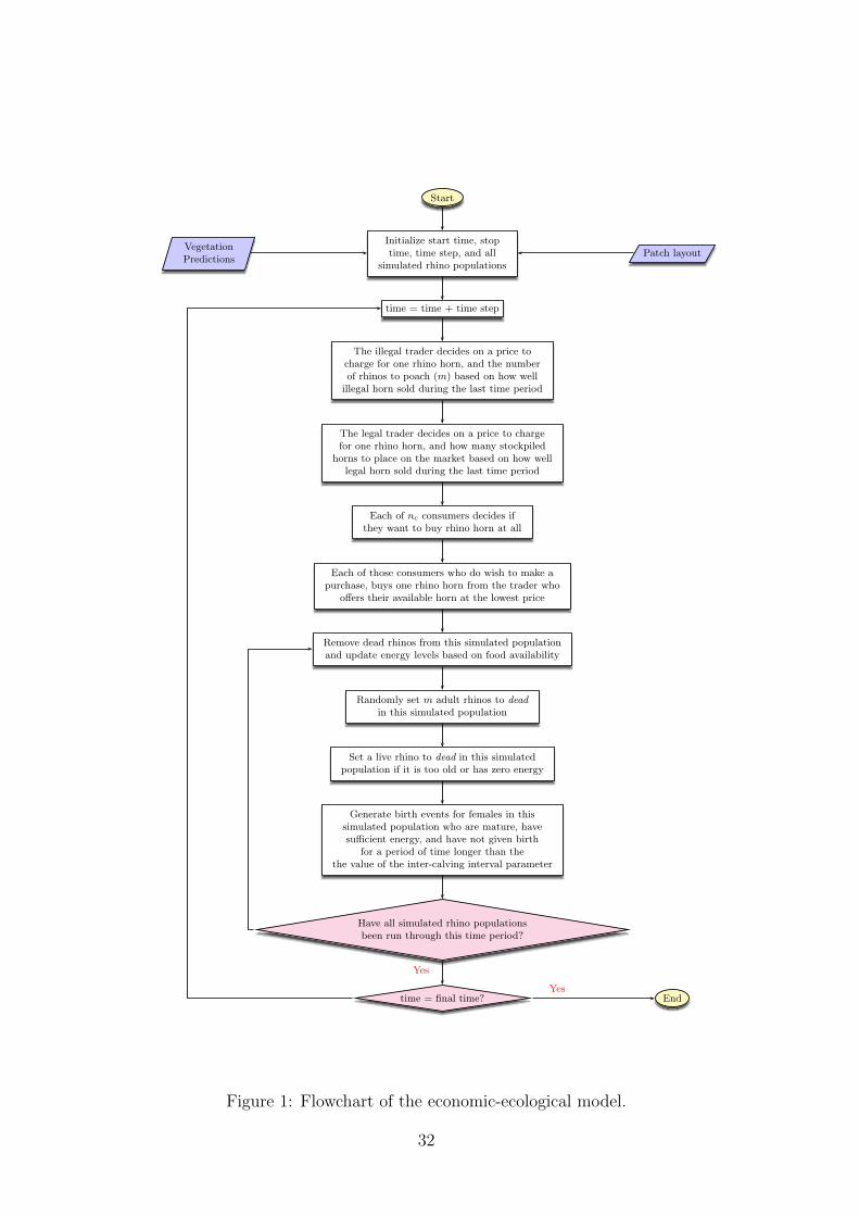
Initialize start time, stoptime, time step, and all
simulated rhino populationsPatch layout
time = time + time step
The illegal trader decides on a price tocharge for one rhino horn, and the numberof rhinos to poach (m) based on how wellillegal horn sold during the last time period
The legal trader decides on a price to chargefor one rhino horn, and how many stockpiled
horns to place on the market based on how welllegal horn sold during the last time period
Each of nc consumers decides ifthey want to buy rhino horn at all
Each of those consumers who do wish to make apurchase, buys one rhino horn from the trader who
offers their available horn at the lowest price
Remove dead rhinos from this simulated populationand update energy levels based on food availability
Randomly set m adult rhinos to dead
in this simulated population
Set a live rhino to dead in this simulatedpopulation if it is too old or has zero energy
Generate birth events for females in thissimulated population who are mature, havesufficient energy, and have not given birth
for a period of time longer than thethe value of the inter-calving interval parameter
Have all simulated rhino populationsbeen run through this time period?
time = final time? End
Yes
Yes
Figure 1: Flowchart of the economic-ecological model.
32
0
20
40
60
80
100
120
140
160
180
2015 2020 2025 2030
Pre
cipi
tatio
n (c
entim
eter
s)
Year
14000
16000
18000
20000
22000
24000
26000
28000
30000
2015 2020 2025 2030
Rhi
no a
bund
ance
Year
Figure 2: Top: predicted KNP precipitation (proxy for new vegetation) (cm); bottom:IBM predictions of rhino abundance under no poaching, ranch-based recreational hunting,and ranch-sourced removals.
33
10
15
20
25
30
2015 2020 2025 2030
Num
ber
of r
hino
s po
ache
d
Year
0
2000
4000
6000
8000
10000
12000
2015 2020 2025 2030
Rhi
no a
bund
ance
Year
0
2000
4000
6000
8000
10000
12000
2015 2020 2025 2030
Rhi
no a
bund
ance
Year
Figure 3: Economic-ecological model time series output under the status quo strategy. Top:number of rhinos poached per week. Second: KNP rhino abundance. Third: ranches rhinoabundance.
34
0
0.2
0.4
0.6
0.8
1
2010 2015 2020 2025 2030 2035 2040 2045
Pro
babi
lity,
ris
k
Year
0
0.2
0.4
0.6
0.8
1
2010 2015 2020 2025 2030 2035 2040 2045
Pro
babi
lity,
ris
k
Year
Figure 4: Local extinction probability (circles), and local extinction risk (squares) underthe status quo strategy. Top: KNP, bottom: ranches.
35